Reexamining Rural Decline: How Changing Rural Classifications Affect Perceived Growth

Georgeanne M. Artz

Assistant Professor of Agricultural Economics and Public Affairs University of Missouri

215 Mumford Hall, Columbia, MO 65203 artzg@missouri.edu

and

Peter F. Orazem

Iowa State University 267 Heady Hall, Ames, Iowa 50011

pfo@iastate.edu

July, 2006

This paper previously circulated under the title “Reexamining Rural Decline: How Changing Ruyral Classifications and Short Time

Frames Affect Perceived Growth”

ISU DEPARTMENT OF ECONOMICS WORKING PAPER #05001

Abstract

This article illustrates the commonly overlooked sample selection problem

inherent in using rural classification methods that change over time due to population changes. Since fast growing rural areas grow out of their rural status, using recent rural definitions excludes the most successful places from the analysis. Average economic performance of the areas remaining rural significantly understates true rural performance. We illustrate this problem using one rural classification system, rural-urban continuum codes. Choice of code vintage alters conclusions regarding the relative speed of rural and urban growth and can mislead researchers regarding magnitudes and signs of factors believed to influence growth. JEL: R11, C24, O18

___________________________ Initial work on this project began when Orazem served as Koch Visiting Professor of Business Economics, University of Kansas School of Business. Advice from seminar participants at the meetings of the American Agricultural Economics Association, and from Cindy Anderson, Will Goudy, Wally Huffman and the referees are gratefully acknowledged.

1

Reexamining Rural Decline: How Changing Rural Classifications Affect Perceived Growth

Abstract

This article illustrates the commonly overlooked sample selection problem

inherent in using rural classification methods that change over time due to population changes. Since fast growing rural areas grow out of their rural status, using recent rural definitions excludes the most successful places from the analysis. Average economic performance of the areas remaining rural significantly understates true rural performance. We illustrate this problem using one rural classification system, rural-urban continuum codes. Choice of code vintage alters conclusions regarding the relative speed of rural and urban growth and can mislead researchers regarding magnitudes and signs of factors believed to influence growth.

JEL: R11, C24, O18

This paper illustrates how conclusions about growth in rural areas of the U.S.

change depending upon when rural status is defined. There are many classification

schemes applied by researchers interested in examining differences in socioeconomic

outcomes between metropolitan and nonmetropolitan areas. Most use counties as a unit

of analysis and are based on measures of population. However, as population changes,

counties’ designations also change over time. This feature is commonly overlooked by

researchers, yet it has important implications for understanding rural growth. The most

successful rural counties in terms of population growth will grow out of the rural

designation and become urban or metropolitan counties. At the same time, the least

successful urban counties may lose enough population to change to rural status. The fact

2

that counties’ status as rural or urban are re-evaluated with each new census creates a

sample selection problem when analyzing patterns of population and economic growth

over time. If rural status is determined by the most recently reported definitions, average

rural population growth will be seriously understated as the fastest growing rural counties

are selected out of and the slowest growing urban counties are sorted into the rural group.

Similar downward bias occurs in measured employment and income growth. By

excluding the most successful counties from the sample, use of the most recent

designations discards valuable information from the very counties from which we have

the most to learn.

We illustrate this sample selection problem using one commonly applied

classification scheme, rural-urban continuum codes. In addition, we show that

conclusions regarding which factors influence growth are also sensitive to the timing of

rural definitions. Specifically, the implications for convergence or divergence in growth

rates across rural counties and conclusions regarding the role of human capital and local

tax and expenditure policies and change when rural status is defined at the end of the

analysis period rather than at the start of the period. Therefore, both academicians and

policy-makers must be careful to use appropriate designations of rural status in evaluating

and formulating prescriptions for rural growth.

These biases are more than just a matter of statistical curiosity. Stories of rural

economic hardship and decline are pervasive in the U.S. and are used to justify

government programs designed to stem the tide of the rural demise. For example,

recently proposed Federal legislation recommends government provision of venture

capital and tax incentives for individuals and businesses to locate in rural areas. These

3

incentives are designed to counter decades of decline in jobs and population that have

resulted in the “decimation of America’s Heartland.”1 While population loss is a very real

and serious problem for some rural counties, due to this consistent measurement error on

the part of researchers, our analysis shows the demise of rural America has been

significantly overstated.

1. DEFINING RURAL STATUS

Rural-urban continuum codes are one common method for classifying counties into

categories based on population data from the U.S. census and, for nonmetropolitan

counties, based on geographic proximity to metropolitan areas. They were developed by

staff at the Economic Research Service in the mid-1970s in order to provide a more

meaningful designation than was possible using rural/urban or metro/non-metro splits

(Hines, et al, 1975).2 The codes were updated in 1983 to reflect population changes

between the 1970 and 1980 Censuses and again in each succeeding decade to reflect the

most current Census data. While the classification categories have remained constant

over time,3 definitional changes have altered how counties are classified. For example, in

the 1974 classification, counties were considered adjacent to a metro if they had a border

contiguous to an SMSA and at least one percent of the county’s population commuted to

the metro’s central county for work. The condition for adjacency was altered in later

versions of the codes, requiring that at least two percent of the employed labor force

commute to the metro’s central county. Another noteworthy definitional change occurred

with the latest rural-urban continuum codes. In the 2000 Census, a significant revision

was made in how rural and urban boundaries were defined, thereby changing the

4

definition of urban population that is applied in the classification scheme. Prior to 2000,

the criteria for defining urban areas were based on a population threshold for places. In

2000, the criteria are based on population density of census blocks and block groups.

One effect of this change is that cities, which previously had no rural population by

definition, may now be comprised of both rural and urban residents. For example, in Des

Moines, Iowa, 100% of the population was designated as urban in 1990; in 2000, 1,155

residents (0.6% of the city’s population) were classified as rural.

Table 1 provides a description of the coding system. We will reference the

codes by the Census year upon which they are based (1970, 1980, 1990, 2000). We

recognize that while all rural counties are nonmetropolitan, not all nonmetropolitan

counties are rural. Nevertheless, many people use the terms rural and nonmetropolitan

interchangeably. Throughout this paper we define rural counties as types 8 and 9,

counties classified as nonmetropolitan, completely rural.

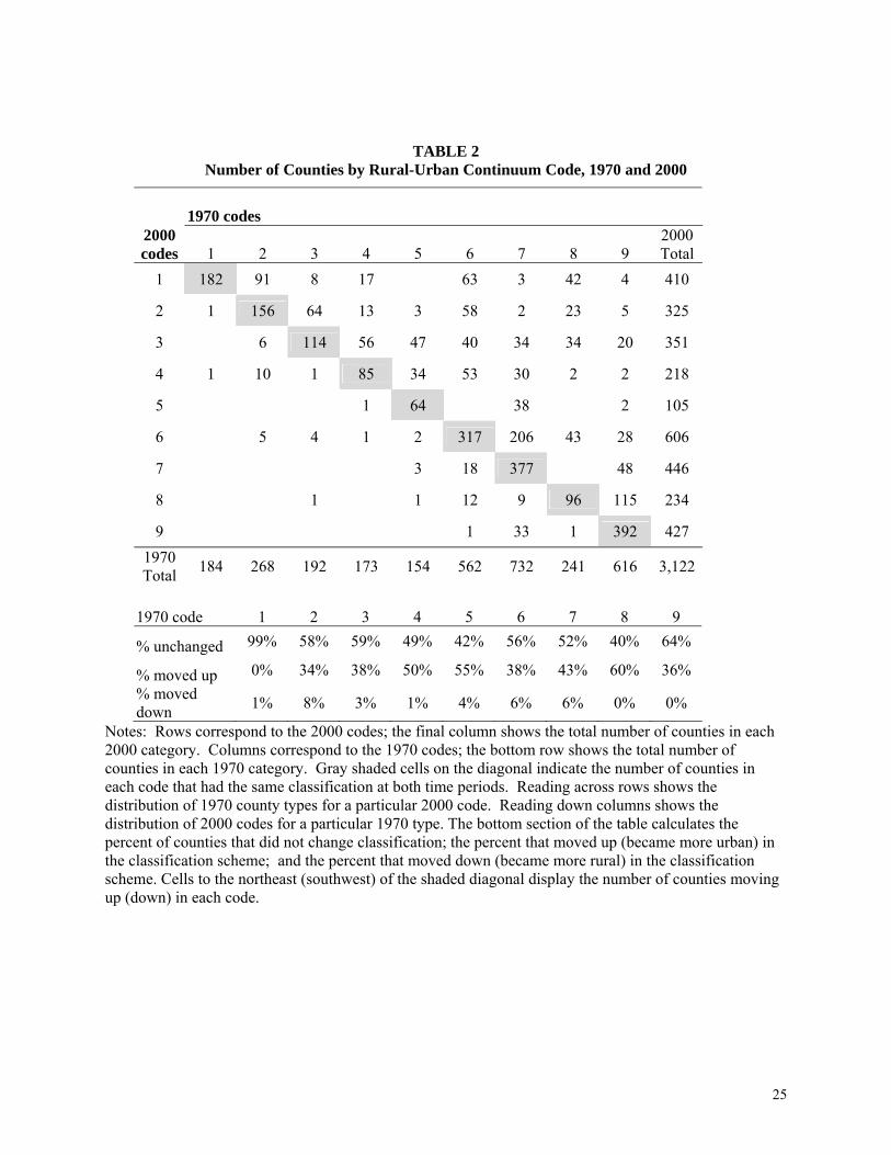
Table 2 shows the number of counties by 1970 and 2000 rural-urban continuum

codes. Each row corresponds to a 2000 rural-urban continuum code designation with the

final column reporting the total number of counties in that 2000 category. Reading

across each row reveals the distribution of 1970 county types for a particular 2000 code.

For example, the first row (2000 type 1) shows that of the 410 metropolitan counties with

over 1 million in population in 2000, 182 were also type 1 in 1970, 91 were type 2 in

1970, 8 were type 3, and so on. Each column corresponds to a 1970 rural-urban

continuum code with the bottom row reporting the total number of counties in that 1970

category. Reading down each column shows the distribution of 2000 codes for a

particular 1970 designation. For example, reading down the column labeled 1970 type 9

5

shows that of the 616 completely rural, nonadjacent counties in 1970, 4 were categorized

as type 1 in 2000, 5 as type 2, 20 as type 3, and so on. Gray shaded cells on the diagonal

indicate the number of counties in each code that had the same classification in both time

periods.

The bottom section of table 2 shows the percent of counties that retained the

same classification or changed classification from their 1970 category. Moving up in the

classification means attaining a code with a smaller number (i.e. moving toward a more

metropolitan classification). Cells to the northeast of the shaded diagonal display the

number of counties moving up in each code. Cells to the southwest of the shaded

diagonal display the number of counties moving down in the classification scheme (i.e.

moving toward a more rural classification).

More than 40% of the counties (1,339 counties) were classified differently in

2000 than in 1970. Of the counties that changed classification, 92% moved “up” in

classification. In general, moving up means gaining population; 89% of the counties that

moved up in the classification scheme experienced population increases between 1970

and 2000. Only 111 counties moved “down” in the classification scheme. Of those

moving down, 41% lost population. A county can move up the classification scheme

without gaining population if a bordering county grows into a metropolitan area.

Similarly, a county can move down the classification scheme despite gaining population

if a bordering county changes from metropolitan to nonmetropolitan status.

Of the 857 counties categorized as nonmetropolitan, completely rural in 1970

(types 8 or 9), 368 or 43% moved up in the continuum. About one-third of these most

rural counties moving up the continuum grew so much that they were classified as

6

metropolitan by 2000. In total, 464 counties or about one-fifth of the nonmetropolitan

counties (codes 4 through 9) became metropolitan counties (codes 1 through 3) by 2000.

While most of these were adjacent to a Standard Metropolitan Statistical Area (SMSA) in

1970, about one quarter (118) were categorized as non-adjacent. Clearly, there is

sufficient movement across classifications that results could be sensitive to the choice of

start-of-period versus end-of-period classifications.

In the study that first used the rural-urban continuum codes, Hines, Brown and

Zimmer (1975) analyzed changes in county social and economic characteristics between

1960 and 1970. The authors recognized the potential problem in using the 1970

classification scheme for their analysis in that “…nonmetro rates of change between 1960

and 1970 for a number of items may be depressed by the inclusion of some rapidly

changing counties in the metro category that were nonmetro at the beginning of the

period (1960). With respect to population growth, for example, newly designated metro

counties grew by 25.3 %, compared with 16.4 % for those that were metro in both 1960

and 1970 and only 4.4 % for those that were nonmetro at both times” (pp. 4)

Nevertheless, they did not adjust their analysis to incorporate a measure of metropolitan

status as of 1960.

Subsequent research has also recognized the problem of changing metropolitan

status and its implications for understanding population trends. Fugitt, Heaton and

Lichter (1988) presented alternative methods for computing nonmetropolitan and

metropolitan population growth rates over time, using county level data. Their analysis

revealed significant differences in the nonmetropolitan growth rate depending upon the

method and definitions applied. For example, they reported nonmetropolitan population

7

growth rates for the 1960s ranging from a 10.9 % increase to a 13.2 % decline. Despite

the large changes in magnitude and even changes in sign, they concluded that “[a]ny

differences in substantive conclusions across the various approaches appear to be largely

a matter of degree rather than kind” (pp. 126).

Even the researchers who acknowledge the problem of changing metropolitan

classifications often fail to correct for the problem. Johnson (1989, pp. 303) stated that

“any effort to examine longitudinal nonmetropolitan demographic trends must address

the issue of metropolitan reclassification,” illustrating that the use of end of the period

rather than start of period classifications reduced the nonmetropolitan growth rate

between 1980 and 1987 by 32 %. Nevertheless, he applied the 1970 classification to

designate nonmetropolitan status for his analysis of historical trends in population growth

between 1930 and 1970.

Fugitt, et al.’s and Johnson’s concern about the potential for changing

metropolitan classification to produce misleading inferences about demographic trends is

largely ignored in the recent literature. An exception is a 2001 article by Andrew

Isserman that distinguishes between rural and formerly rural counties. Isserman

illustrates how dramatically conclusions about rural population growth and economic

success change when rural is defined by the set of counties classified as nonmetropolitan

in 1950 relative to a definition of rural based on the 2000 Census. “Today, some 71

million people, one-fourth of the U.S. population, live in what was rural America in 1950

but is considered urban America today” (pp. 41).

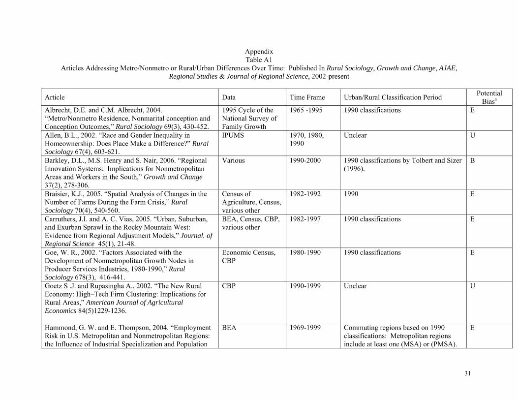
A number of recent articles appearing in leading academic journals with a rural

development focus examine metro/non-metro differences in social and economic trends

8

(See Appendix table A1 for a list of these articles). Most use rural-urban continuum

codes to classify areas or individuals as rural/urban or metro/non-metro, yet in most the

timing of the classification scheme is not discussed. Of twenty-six articles identified, six

used beginning-of-period codes, eleven used end-of-period codes, eight did not identify

the code used, and one allowed a county’s status to change over time.

When authors use the metro/non-metro status reported by the government, they

will, often inadvertently, be using the most recent code vintage. For example, three of the

studies mentioned above used longitudinal data from the Current Population Survey

(CPS) in which an individual’s residence is classified as metropolitan or nonmetropolitan.

The CPS uses current rural-urban continuum code designations, effectively allowing rural

status to change over time. Since a county may change status over time, an individual in

the survey may migrate from rural to nonmetropolitan to metropolitan areas without

changing residence. Unfortunately, there is no obvious way to correct for changing rural

designations in time series evaluations of the CPS data because county of residence is not

identified. These seemingly minor points can lead to very misleading conclusions about

changes in rural areas. For example, it is readily assumed that declining rural population

has resulted from people moving out of rural areas and into the cities. Yet, one-third of

1950 rural residents became urban dwellers without leaving home (Isserman, 2001).

2. MEASURING RURAL GROWTH

How rural is defined has important implications for measuring growth. Total U.S.

population increased 38% between 1970 and 2000. Population in the set of counties

defined as rural in 1970 grew 41% between 1970 and 2000, faster than the national rate.

Population in those counties classified as rural in 2000 grew only 13% over this period,

9

about one-third as much as the national increase. Clearly, these two figures paint very

different pictures about rural growth over the past three decades.

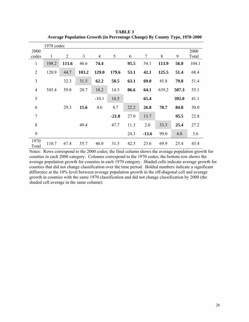
Table 3 presents the average population growth for U.S. counties classified by

1970 and 2000 rural-urban continuum codes. The shaded cells indicate the average for

counties that did not change classification over that period. Cells to the southwest of the

shaded diagonal display average growth rates for counties that moved down the

classification scheme. For example, 1970 type 7 counties that became type 9 counties in

2000 suffered an average population loss of 13.6 %. Cells to the northeast of the shaded

diagonal display average growth rates for counties that moved up in the scheme. For

instance, counties that were classified as type 9 in 1970 but changed to type 7 in 2000

grew on average 95.5 %. Bolded numbers indicate that the average population growth

for counties in that off-diagonal cell is significantly different from the shaded number in

that column showing the average growth of counties that were in the same classification

in 1970 but did not change type.

The average population growth for all counties was 43.4% from 1970 to 2000. In

general, counties that moved up the classification scheme experienced faster population

growth and counties that moved down in the classification scheme grew more slowly

when compared to counties whose type did not change. For six of the nine county types,

use of the 2000 classification understates population growth. Using the 2000 codes, one

would conclude that the average population growth for rural, non-adjacent counties (type

9) was 4% when in fact, average population growth in these counties was more than six

times that rate, 25.4%, over the 1970-2000 period. Using the 2000 codes not only

excludes those type 9 counties which grew enough to be re-classified between 1970 and

10

2000, but it also includes those counties that moved down to type 9, in many cases

because they suffered population losses. Similarly, the growth rate for completely rural

adjacent counties (type 8) was 70%, using the 1970 classification, 1.6 times larger than

the 27% obtained using the 2000 codes (27%). For three of the nine county types (2, 4,

and 5), population growth is overstated when the 2000 codes are applied. Population in

the largest nonmetropolitan, non-adjacent counties (type 5) grew on average 31% from

1970 to 2000. When the 2000 codes are used, however, the implied growth rate was

41%, as fast-growing, formerly rural counties are added to the type 5 group.

Population more than doubled in 390 counties between 1970 and 2000. Over

half of these (231) were designated nonmetropolitan in 1970, with about one-fourth (103)

classified as completely rural. Of this set of fastest growing counties, two-thirds changed

rural-urban continuum code designation, moving up in the classification scheme. More

than half of the completely rural counties in this group (55 of 103) lost their rural status

by 2000.

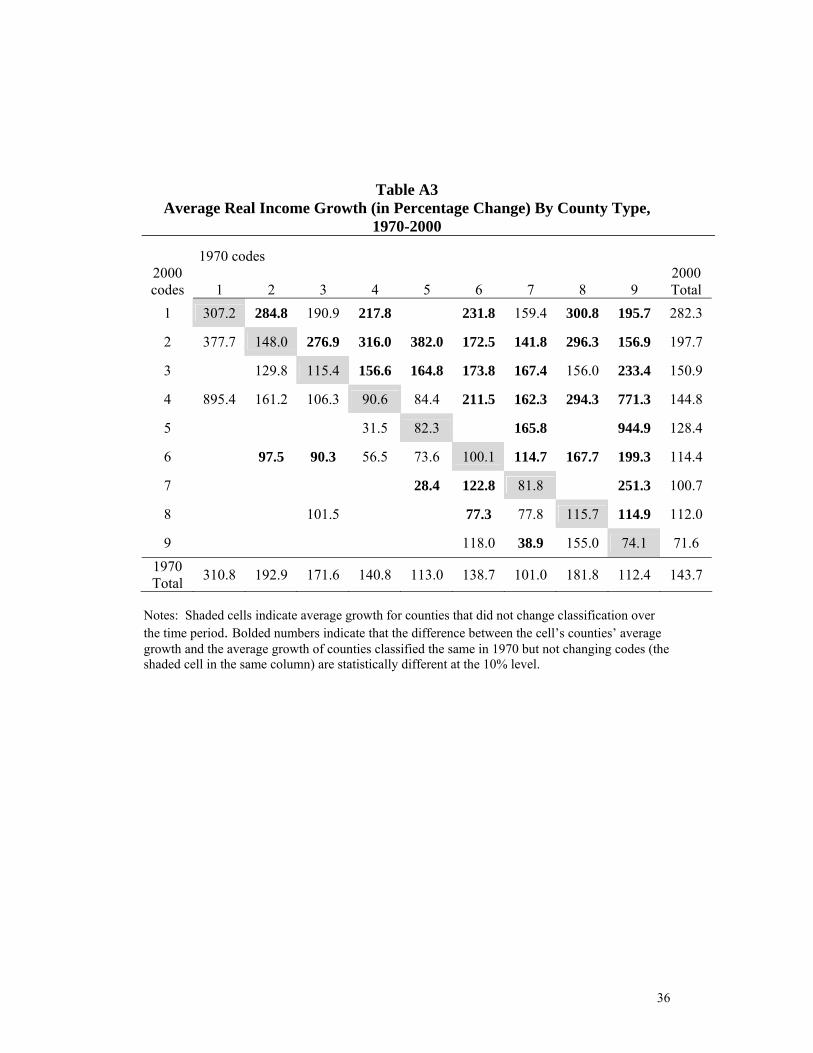
Similar patterns emerge when comparing county employment and income growth

when 2000 rural designations are used rather than 1970 designations. 4 Use of the 2000

codes dramatically understates rural growth which can lead to incorrect inferences

regarding the relative success of rural and urban counties. For example, Ghelfi’s (2002)

recent report of widening urban-rural income gaps is found when 2000 rural designations

are used, but are reversed when we use the 1970 designations..

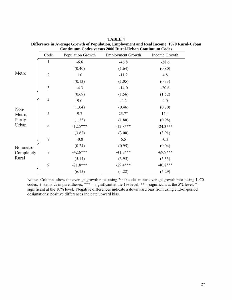
Table 4 summarizes the differences in average growth rates of population,

employment and real income using the 1970 and 2000 rural-urban continuum codes. To

illustrate how to read the table, the average population growth for type 1 counties

11

according to the 1970 classification was 110.7% compared to 104.1% using the 2000

classification. The difference is -6.6%, suggesting that the use of 2000 rural-urban

continuum codes biases downward the implied population growth of the largest counties.

The t-statistic shows that the bias is not statistically different from zero.5

For six of the nine county designations, the direction of the bias is consistent

across all three growth indicators. For rural areas, the bias is large, negative and

significant. For metropolitan areas, the bias is most often negative but small and never

statistically significant. The direction of bias varies for nonmetropolitan urban counties.

Most noticeably, growth is consistently inflated in type 5 counties when the 2000

designations are used.

The implication of table 4 is that rural growth is consistently understated relative

to its true value when end-of-period rural designations are used. Use of the 2000 rural-

urban continuum codes sorts out the fastest growing rural counties and sorts in shrinking

urban counties. The bias in measured rural growth is very large, ranging from 22% to

70% depending on growth measure and county type. Use of the 2000 designations leads

to the false conclusion that rural counties have much slower than average growth,

however measured. Use of the 1970 designations reverses these conclusions.

3. REGRESSION ANALYSIS OF THE DETERMINANTS OF COUNTY

GROWTH

In addition to creating problems in reporting and analyzing trends for

metropolitan and nonmetropolitan counties, the choice of end-of-period versus start-of-

period rural-urban continuum code classifications can have a dramatic effect on

12

conclusions regarding the determinants of local growth. To illustrate, we estimated the

Deller, et al. (2001) reduced form version of the Carlino and Mills (1987) model,

regressing the rural county growth rates described above on human capital measures,

policy variables, and environmental factors commonly used in this literature.6

In this model equilibrium employment, population and per capita income are

simultaneously determined in a spatial general equilibrium model in which both

households and firms are geographically mobile. Households seek to maximize utility,

which in its indirect form is a function of wages, rents and a mix of other site-specific

characteristics such as non-market amenities and local fiscal policies. Local taxes are

expected to reduce utility since a higher tax incidence reduces both consumption

expenditures and government services.

Firms maximize profit which depends on wages, rents and other site specific

attributes. Firm productivity varies across locations due to regional differences in labor

supply, transportation costs, agglomeration economies and local fiscal policy.

Interregional movement of firms and households occurs until utility levels and profit

levels are equalized across locations.

Equilibrium levels of employment and population, E*, P* and I* are functions of

county employment, E, county population, P, and county per capita income, I, as well as

a vector of partially or fully overlapping exogenous location-specific attributes, Z. This

vector includes variables such as climate, crime rates, human capital stocks and local

fiscal policy. We suppress county subscripts for ease of exposition.

(1) 1 2* * *E E EE P I Zα α β= + +

13

(2) 1 2* * *P P PP E I Zα α β= + +

(3) ZEPI III βαα ++= *** 21

Population, employment and income are assumed to adjust their equilibrium levels with

substantial lags:

(4) )*( 11 −− −+= tEtt EEEE λ

(5) )*( 11 −− −+= tPtt PPPP λ

(6) )*( 11 −− −+= tItt IIII λ

where the subscript t references time periods and λE, λP and λI represent speed of

adjustment parameters. Bringing the lagged values of E, P and I to the left hand side of

the equation and substituting for their equilibrium values yields the following three

equation system:

(7) 1 1 1 2t t E t E E E E E EE E E E P I Zλ λ α λ α λ β− −Δ = − = − + + +

(8) 1 1 1 2t t P t P P P P P PP P P P E I Zλ λ α λ α λ β− −Δ = − = − + + +

(9) ZEPIIII IIIIIItItt βλαλαλλ +++−=−=Δ −− 2111

In reduced form, the model becomes:

(7’) 0 1 1 2 1 3 1E E t E t E t EE E P I Zγ γ γ γ δ− − −Δ = + + + +

(8’) ZEIPP PtPtPtPP δγγγγ ++++=Δ −−− 1312110

(9’) ZPEII ItItItII δγγγγ ++++=Δ −−− 1312110

14

where population, employment and income growth are functions of the lagged values of

these measures and Z. We estimate the reduced form model under different rural-urban

continuum code regimes to examine if the results are sensitive to the choice of start-of

period or end-of-period rural status. The reduced form parameters γ represent the effect

on the equilibrium values of E, P and I from a change in the exogenous regressors after

all feedback effects have occurred. The estimate of γ1i is of particular interest in that a

positive coefficient suggests that counties are diverging in size while a negative

coefficient implies that counties are converging.

Recent research demonstrates that economic growth is correlated across counties

roughly within commuting distance of one another (Wheeler 2001; Khan, Orazem and

Otto 2001). This suggests there is potential spatial correlation in growth rates across

counties in the sample. To account for this, we allow for spatial error dependence by

estimating clustered standard errors which assume correlation among counties in the

same economic region, but no correlation across regions. 7

The exogenous variables are summarized in table 5. We include 1970 measures

of population, employment and income in natural logs to control for initial conditions and

to examine whether growth among rural counties tends to converge or diverge.8 Amenity

measures obtained from the USDA’s Economic Research Service are used to control for

time invariant climatic differences across regions. We use start-of-period values for the

percent of the county population with a high school degree and percent with a college

education or higher to measure initial human capital endowments. Start-of-period values

of the percent of the population aged sixty-five or older and the percent non-white

measure demographic characteristics that may affect both labor supply and local demand

15

for goods and services. Start-of-period local government expenditures and taxes per

employee measure variation in local fiscal policy that may deter or encourage growth.

We include regional dummies as well as the natural log of the county area in square miles

to control for variation in county size across the U.S. A dummy variable indicates

adjacency to a metropolitan area.

The dependent variables are log differences of county population, employment

and average wages between 1970 and 2000. We use average wages rather than per capita

income because wages are the more theoretically appropriate measure of labor

productivity, whereas income includes proprietor’s income earned outside the county and

other income transfers. Moreover, wages are the better signal of the relative return to

working in the county, whereas county per capita income will reflect the number of

children and retired in the population which will vary for reasons other than economic

growth.

We defined the sample of rural counties in two ways. The first, based on the

1970 rural-urban continuum code definitions, results in a sample of 847 rural counties.

These counties are shaded in black and grey in figure 1. The second, derived from the

2000 codes, produces a sample of 655 rural counties. These counties are indicated by

cross hatch-shading and black in the figure.

Table 6 reports the regression results correcting for spatial random effects. The

first column reports the regression results for the population growth equations using the

1970 definitions to define the sample of rural counties. The second column reports the

results of the same regression using the 2000 definitions to define the sample. The third

column reports the level of significance of a test of the difference between the

16

coefficients in each equation.9 In addition, we computed a joint test of the null

hypothesis that all coefficients were equal across the two regressions. The F-test statistic

is reported in the bottom row of the table. Columns 4-6 report similar results for the

employment growth equations. Results for the income growth equations appear in

columns 7-9.

In all cases, the null hypothesis that the coefficients are equal across the

regressions based on the 1970 and 2000 rural definitions was rejected. There are notable

differences in the magnitudes and significance levels of coefficients between the two

samples, several of which are key to assessments of growth strategies for rural counties.

The most striking difference between the two samples is the implication for the

convergence among counties in the sample. The potential problem of sample selection

for establishing convergence or divergence in growth is well recognized in the literature

on convergence among countries. Studies reporting income convergence across nations

by William Baumol (1986) and Angus Maddison (1983) were criticized for using an ex

post sample of countries. Lant Pritchett argues:

Defining the set of countries as those that are the richest now almost guarantees the finding of historical convergence, as either countries are rich now and were rich historically, in which case they all have had roughly the same growth rate (like nearly all of Europe) or countries are rich now and were poor historically (like Japan) and hence grew faster and show convergence. However, examples of divergence, like countries that grew much more slowly and went from relative riches to poverty (like Argentina) or countries that were poor and grew so slowly as to become relatively poorer (like India), are not included in the samples of “now developed” countries that tend to find convergence (1997, p. 6) This analysis provides an analogous situation in which sorting might lead to

artificial evidence of convergence. Counties considered rural in 2000 either have not

grown since 1970 or have become rural because they lost population since 2000.

17

Meanwhile, counties which grew out of their rural status are, by definition, excluded

from the sample.

In this analysis, there is significant evidence of diverging population and

employment growth favoring the largest counties when start-of-period county

designations are used to define the sample. Use of the end-of-period sample that sorts out

the fastest growing rural counties eliminates the finding of divergent employment and

population growth and even causes the estimate of γ1E to reverse sign. Regardless of

rural definition, there is strong evidence that average wages converge across counties

over this time period, a finding consistent with an equilibrium model of the labor market

in which firms and households freely migrate.

Conclusions regarding the estimated effect of human capital and fiscal policies

on growth are also sensitive to the choice of rural definition. Higher proportions of high

school graduates led to slower population and employment growth in both samples.

However, the incremental effect of college graduates on growth is consistently positive

and larger when the 1970 rural designation is used, although it is significant only in the

employment growth regression. Higher expenditures raise population and employment

growth significantly using either rural sample, but higher taxes have a significant impact

on employment growth only when the 2000 sample is used. Higher taxes significantly

lower wage growth in both samples.

Another difference is seen in the role of a county’s age composition for

employment growth. The end-of-period sample suggests that higher initial proportions of

retirees (age 65 and over) led to faster employment growth, a result that does not hold in

when the 1970 rural designations are used. In addition, using the 2000 definition

18

understates the importance of metropolitan adjacency for all three measures of rural

growth.

Some conclusions about the data do not change drastically as a result of changing

rural-urban continuum code classifications. The role of a rural county’s race

composition does not differ between the two samples nor do regional growth patterns.

Using the start-of-period sample shows that rural counties in the northeastern U.S.

experienced relatively faster population and employment growth compared with counties

in the Midwest, while the end-of-period sample indicates no significant difference. In

general, however, these coefficients are not statistically different across equations. The

various amenity measures generally have consistent signs and significance across the two

samples in directions conforming to presumptions.

When the model is estimated using ordinary least squares, ignoring the potential

spatial correlation, the model produces identical coefficients but smaller standard errors.10

As a consequence, many of the sign changes in table 6 are also now statistically

significant. This suggests that misleading conclusions about rural growth are further

compounded by model specification issues, in this case, failing to account for spatial

correlation.

4. CONCLUSION

This analysis illustrates the potential for bias when analyzing rural and urban

differences over time. Using end-of-period designations to define rural status

significantly understates the economic performance of rural counties over the past three

decades. Population growth between 1970 and 2000 in the most rural counties is

understated by 22% or more when 2000 designations instead of 1970 designations are

19

used to define the set of rural counties. Average employment growth is underestimated by

30 percentage points or more and average income growth by more than 40 percentage

points.

Furthermore, using end-of-period rural-urban continuum code can yield

misleading conclusions about which factors affect growth. Divergence in population and

employment growth among rural counties is significantly understated when the end-of-

period sample is used, since counties that grow the fastest are excluded from this sample.

Conclusions regarding the role of factors that policy can affect also change according to

the specification. For example, beginning-of-period sample results suggest that providing

higher levels of public services is more important for population and employment growth

than minimizing tax burdens. Also, in the beginning-of-period sample, higher

proportions of college graduates play a positive role in employment growth. This

suggests that rural counties should be concerned about “brain drain” or the loss of

college-educated residents from rural areas. Both these policy implications are weakened

or completely overlooked when end-of-period samples are used. Given these findings,

we recommend that beginning-of-period definitions always be applied when analyzing

rural economic growth.

Understanding how and why economic growth occurs in rural America is a

challenging, yet vital part of designing effective policies at both the federal and local

level. Confounding this challenge is the fact that the most successful rural counties are

no longer rural. If these counties are ignored in analyzing factors that help rural counties

grow, we are disregarding the very group of counties that offers the most successful

cases. If instead, we define rural status at the outset, we obtain both a more encouraging

20

outlook regarding the prospects for rural growth and better information regarding the

factors that can lead to rural expansion.

21

Endnotes

1 Quoting the web site of Senator Byron L. Doran. The news release supporting the New Homestead Act contend that, “nearly 70% of rural counties on the Great Plains have seen their populations shrink by an average of about a third.” That statistic should more accurately be stated as, “70% of counties remaining rural …have experienced population decline.” See http://dorgan.senate.gov/legislation/homestead/homesteadbrochure.pdf. 2 A number of classification schemes have been developed to distinguish rural from urban or metropolitan from non-metropolitan areas. Nearly all of these are subject to what Isserman calls the “county trap.” “The problem begins when we, as researchers and policy makers, knowingly fall into the county trap by referring to metropolitan counties as urban and all other counties as rural. Doing so ignores the blending of urban and rural populations within counties, the presence of rural people and places in metropolitan areas and urban people and places in nonmetropolitan counties, and the intent of the metropolitan system to measure urban-rural integrations, not urban-rural differentiation” (2005, p. 470). While we recognize this as a serious issue for defining rural as well, our analysis focuses on the implications of classification scheme vintages. 3 The only exception is that in the most recently released Beale codes, the central and fringe counties of major metropolitan areas (types 0 and 1) have been consolidated into one category. To make our results comparable over time, we aggregate classifications 0 and 1 into a single class. 4 The results that replicate the analysis of table 3 using growth in aggregate income and in employment are available in Appendix tables A2 and A3. The differences are summarized in table 4. 5 Use of beginning-of-period and end-of-period metropolitan status defines two different samples of rural counties, which can be viewed as a sample selection or sorting problem. Use of a t-test to determine statistical significance is appropriate given this view of the data. 6 These regressions are designed to explore whether the results are sensitive to the sorting arising from the choice of beginning-of-period or end-of-period Beale codes. While we have attempted to include measures typically used in the growth literature, we recognize that there is disagreement as to the most appropriate model for describing economic growth. 7 Regions are defined by the Bureau of Economic Analysis’ economic areas, which are designed to encompass regional centers and their surrounding counties. The definitions are based on commuting data and newspaper circulation (Partridge, et al. 2006). The t-statistics we report in the tables are cluster-consistent t-statistics or Rogers t-statistics (Primo, Jacobsmeier and Milyo 2006).

22

8 The log of population in 1970 and the log of employment in 1970 are highly correlated (ρ = 0.92) ; therefore the log of 1970 employment is excluded from the population and income growth regressions, while the log of 1970 population is excluded from the employment growth regressions. 9 To conduct this test, we created a dummy variable which took a value of 1 if the county was rural in both 1970 and 2000 and zero otherwise. This variable was interacted with each of the explanatory variables and added to the set of regressors used in the growth regressions using the 1970 sample selection criteria. The coefficient on the dummy variable interaction terms can be interpreted as a measure of the change in the coefficient between the 1970-defined and 2000-defined samples of rural counties. The joint test of significance across all the interacted variables is interpretable as the global test of stability on coefficients between the two sets of counties. 10 These results are available in Appendix table A4.

23

References

Baumol, W., 1986. “Productivity Growth, Convergence, and Welfare: What the Long-Run Data Show,”

American Economic Review 79(5),1072-1085. Carlino, G. and E. Mills, 1987. “The Determinants of County Growth.” Journal of Regional Science 27,

39-54. Deller, S., T. Tsai, D. Marcouiller, and D. English, 2001. “The Role of Amenities and Quality of Life in

Rural Economic Growth,” American Journal of Agricultural Economics 83(2),352-365. Fugitt, G., T. Heaton, and D. Lichter, 1988. “Monitoring the Metropolitanization Process,” Demography

25(1), 115-128. Ghelfi, L. M., 2002. “Rural Earnings up in 2000, but Much Less than Urban Earnings,” Rural America

17(4), 78-83. F. K. Hines, D. L. Brown, and J. M. Zimmer. 1975. Social and Economic Characteristics of the

Population in Metro and Nonmetro Counties: 1970, Economic Research Service. Isserman, A. 2001. “Competitive Advantages of Rural American in the Next Century,” International

Regional Science Review 24(1), 38-58. Isserman, A. 2005. “In the National Interest: Defining Rural and Urban Correctly in Research and Public

Policy,” International Regional Science Review 28(4), 465-499. Johnson, K., 1989. “Recent Population Redistribution Trends in Nonmetropolitan America,” Rural

Sociology 54(3), 301-326. Khan, R., P. Orazem, and D. Otto. 2001. “Deriving Empirical Definitions of Spatial Labor Markets: The

Roles of Competing versus Complementary Growth,” Journal of Regional Science. 41, 735-756. Maddison, A. 1983. “A Comparison of Levels of GDP Per Capita in Developed and Developing

Countries, 1700-1980,” Journal of Economic History 43(1), 27-41. Partridge, M., D. Rickman, K. Ali and M. Rose Olfert, 2005. “Does the New Economic Geography

Explain U.S. Core-Periphery Population Dynamics?” Paper prepared for the 45th Annual Meetings of the Southern Regional Science Association, March 30-April 1, St. Augustine, FL.

Prichett, L., 1997. “Divergence, Big Time,” Journal of Economic Perspectives 11(3), 3-17. Primo D., M. Jacobsmeier and J. Milyo. 2006. “Estimating the Impact of State Policies and Institutions

with Mixed-Level Data.” Department of Economics, University of Missouri, WP 06-03, February.

Wheeler, C. H. 2001. “A Note on the Spatial Correlation Structure of County-Level Growth in the U.S.,”

Journal of Regional Science 41,433-449.

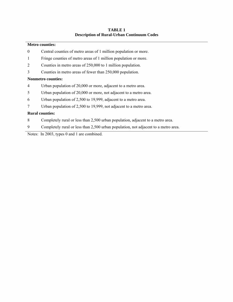
TABLE 1 Description of Rural-Urban Continuum Codes

Metro counties: 0 Central counties of metro areas of 1 million population or more. 1 Fringe counties of metro areas of 1 million population or more. 2 Counties in metro areas of 250,000 to 1 million population. 3 Counties in metro areas of fewer than 250,000 population.

Nonmetro counties: 4 Urban population of 20,000 or more, adjacent to a metro area. 5 Urban population of 20,000 or more, not adjacent to a metro area. 6 Urban population of 2,500 to 19,999, adjacent to a metro area. 7 Urban population of 2,500 to 19,999, not adjacent to a metro area.

Rural counties: 8 Completely rural or less than 2,500 urban population, adjacent to a metro area. 9 Completely rural or less than 2,500 urban population, not adjacent to a metro area.

Notes: In 2003, types 0 and 1 are combined.

25

TABLE 2 Number of Counties by Rural-Urban Continuum Code, 1970 and 2000

1970 codes 2000 codes 1 2 3 4 5 6 7 8 9

2000 Total

1 182 91 8 17 63 3 42 4 410

2 1 156 64 13 3 58 2 23 5 325

3 6 114 56 47 40 34 34 20 351

4 1 10 1 85 34 53 30 2 2 218

5 1 64 38 2 105

6 5 4 1 2 317 206 43 28 606

7 3 18 377 48 446

8 1 1 12 9 96 115 234

9 1 33 1 392 427 1970 Total 184 268 192 173 154 562 732 241 616 3,122

1970 code 1 2 3 4 5 6 7 8 9

% unchanged 99% 58% 59% 49% 42% 56% 52% 40% 64%

% moved up 0% 34% 38% 50% 55% 38% 43% 60% 36% % moved down 1% 8% 3% 1% 4% 6% 6% 0% 0%

Notes: Rows correspond to the 2000 codes; the final column shows the total number of counties in each 2000 category. Columns correspond to the 1970 codes; the bottom row shows the total number of counties in each 1970 category. Gray shaded cells on the diagonal indicate the number of counties in each code that had the same classification at both time periods. Reading across rows shows the distribution of 1970 county types for a particular 2000 code. Reading down columns shows the distribution of 2000 codes for a particular 1970 type. The bottom section of the table calculates the percent of counties that did not change classification; the percent that moved up (became more urban) in the classification scheme; and the percent that moved down (became more rural) in the classification scheme. Cells to the northeast (southwest) of the shaded diagonal display the number of counties moving up (down) in each code.

26

TABLE 3 Average Population Growth (in Percentage Change) By County Type, 1970-2000

1970 codes 2000 codes 1 2 3 4 5 6 7 8 9

2000 Total

1 108.2 111.6 46.6 74.4 95.5 54.1 113.9 56.0 104.1

2 120.9 44.7 103.2 129.0 179.6 53.1 42.1 125.5 51.4 68.4

3 32.3 31.5 62.2 58.5 63.1 69.0 45.8 79.8 51.4

4 545.4 59.8 20.7 18.2 14.5 86.6 64.1 639.2 507.3 55.1

5 -10.1 16.5 65.4 392.0 41.1

6 29.3 15.6 4.6 4.7 22.2 26.8 70.7 84.8 30.0

7 -21.8 27.0 13.7 95.5 22.8

8 49.4 47.7 11.3 2.0 33.3 25.4 27.2

9 24.3 -13.6 99.0 4.8 3.6 1970 Total 110.7 67.4 55.7 46.0 31.3 42.5 23.6 69.9 25.4 43.4

Notes: Rows correspond to the 2000 codes; the final column shows the average population growth for counties in each 2000 category. Columns correspond to the 1970 codes; the bottom row shows the average population growth for counties in each 1970 category. Shaded cells indicate average growth for counties that did not change classification over the time period. Bolded numbers indicate a significant difference at the 10% level between average population growth in the off-diagonal cell and average growth in counties with the same 1970 classification and did not change classification by 2000 (the shaded cell average in the same column).

27

TABLE 4 Difference in Average Growth of Population, Employment and Real Income, 1970 Rural-Urban

Continuum Codes versus 2000 Rural-Urban Continuum Codes Code Population Growth Employment Growth Income Growth

1 -6.6 -46.8 -28.6 (0.40) (1.64) (0.80)

2 1.0 -11.2 4.8 (0.13) (1.05) (0.33)

3 -4.3 -14.0 -20.6 (0.69) (1.56) (1.52)

4 9.0 -4.2 4.0 (1.04) (0.46) (0.30)

5 9.7 23.7* 15.4 (1.25) (1.80) (0.98)

6 -12.5*** -12.8*** -24.3*** (3.62) (3.00) (3.91)

7 -0.8 6.5 -0.3 (0.24) (0.95) (0.04)

8 -42.6*** -41.8*** -69.9*** (5.14) (3.95) (5.33)

9 -21.8*** -29.4*** -40.8*** (6.15) (4.22) (5.29)

Notes: Columns show the average growth rates using 2000 codes minus average growth rates using 1970 codes; t-statistics in parentheses; *** = significant at the 1% level; ** = significant at the 5% level; *= significant at the 10% level. Negative differences indicate a downward bias from using end-of-period designations; positive differences indicate upward bias.

Metro

Non- Metro, Partly Urban

Nonmetro, Completely Rural

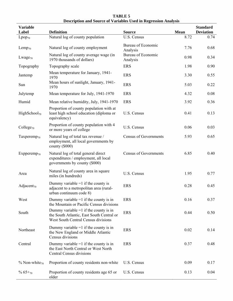
TABLE 5 Description and Source of Variables Used in Regression Analysis

Variable Label Definition Source Mean

Standard Deviation

Lpop70 Natural log of county population U.S. Census 8.72 0.74

Lemp70 Natural log of county employment Bureau of Economic Analysis 7.76 0.68

Lwage70 Natural log of county average wage (in 1970 thousands of dollars)

Bureau of Economic Analysis 0.98 0.34

Topography Topography scale ERS 1.98 0.90

Jantemp Mean temperature for January, 1941-1970 ERS 3.30 0.55

Sun Mean hours of sunlight, January, 1941-1970 ERS 5.03 0.22

Julytemp Mean temperature for July, 1941-1970 ERS 4.32 0.08

Humid Mean relative humidity, July, 1941-1970 ERS 3.92 0.36

HighSchool70 Proportion of county population with at least high school education (diploma or equivalency)

U.S. Census 0.41 0.13

College70 Proportion of county population with 4 or more years of college U.S. Census 0.06 0.03

Taxperemp70 Natural log of total tax revenue / employment, all local governments by county ($000)

Census of Governments 5.93 0.65

Expperemp70 Natural log of total general direct expenditures / employment, all local governments by county ($000)

Census of Governments 6.85 0.40

Area Natural log of county area in square miles (in hundreds) U.S. Census 1.95 0.77

Adjacent70 Dummy variable =1 if the county is adjacent to a metropolitan area (rural-urban continuum code 8)

ERS 0.28 0.45

West Dummy variable =1 if the county is in the Mountain or Pacific Census divisions

ERS 0.16 0.37

South Dummy variable =1 if the county is in the South Atlantic, East South Central or West South Central Census divisions

ERS 0.44 0.50

Northeast Dummy variable =1 if the county is in the New England or Middle Atlantic Census divisions

ERS 0.02 0.14

Central Dummy variable =1 if the county is in the East North Central or West North Central Census divisions

ERS 0.37 0.48

% Non-white70 Proportion of county residents non-white U.S. Census 0.09 0.17

% 65+70 Proportion of county residents age 65 or older

U.S. Census 0.13 0.04

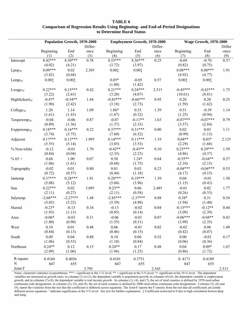
TABLE 6

Comparison of Regression Results Using Beginning- and End-of-Period Designations to Determine Rural Status

Population Growth, 1970-2000 Employment Growth, 1970-2000 Wage Growth, 1970-2000

Beginning

(1) End (2)

Differ-ence (3)

Beginning (4)

End (5)

Differ-ence (6)

Beginning (7)

End (8)

Differ-ence

(9) Intercept 8.42***

(4.02) 8.30*** (4.21)

0.78 8.53*** (3.72)

8.36*** (3.97)

0.25 -0.69 (0.82)

-0.70 (0.75)

0.37

Lpop70 0.09*** (3.82)

0.02 (0.68)

2.30† 0.00‡ 0.00‡ 0.08*** (4.92)

0.08*** (4.77)

1.91

Lemp70 0.00‡ 0.00‡ 0.05* (1.80)

-0.05 (1.42)

0.57 0.00‡ 0.00‡

Lwage70 0.22*** (3.22)

0.15*** (2.63)

0.42 0.21*** (3.20)

0.24*** (4.07)

2.51† -0.45*** (10.61)

-0.43*** (8.81)

1.75

HighSchool70 -0.47* (1.90)

-0.54** (2.42)

1.44 -0.83*** (3.18)

-0.66*** (2.73)

0.95 0.20 (1.59)

0.20 (1.62)

0.25

College70 1.20 (1.61)

1.14 (1.43)

1.09 1.86* (1.87)

0.35 (0.32)

1.39 0.51 (1.25)

-0.39 (0.94)

1.14

Taxperemp70 -0.04 (0.89)

-0.06 (1.36)

0.87 -0.07 (1.37)

-0.11** (2.33)

1.63 -0.07*** (3.57)

-0.07*** (2.84)

0.79

Expperemp70 0.18*** (3.74)

0.16*** (3.75)

0.22 0.37*** (7.60)

0.31*** (6.52)

0.00 0.02 (0.99)

0.03 (1.13)

1.11

Adjacent 0.17*** (5.55)

0.13*** (5.14)

1.99† 0.14*** (3.85)

0.11*** (3.53)

1.19 0.04** (2.29)

0.03* (1.68)

2.12†

% Non-white -0.12 (0.84)

-0.01 (0.04)

1.70 -0.42** (2.35)

-0.43** (2.23)

0.10 0.25*** (4.86)

0.29*** (4.37)

1.59

% 65 + 0.68 (1.06)

1.00 (1.61)

0.07 0.50 (0.68)

1.24* (1.75)

0.64 -0.55** (2.10)

-0.64** (2.15)

0.57

Topography -0.02 (0.72)

0.01 (0.57)

0.80 0.01 (0.44)

0.03 (1.18)

0.23 -0.04*** (4.17)

-0.04*** (4.15)

0.53

Jantemp 0.37*** (5.08)

0.28*** (5.12)

1.91 0.28*** (5.04)

0.19*** (3.96)

1.39 0.04 (1.15)

-0.01 (0.43)

1.58

Sun 0.22*** (2.11)

0.02 (0.27)

3.09† 0.23** (2.11)

0.06 (0.58)

2.48† -0.01 (0.26)

0.02 (0.33)

1.77

Julytemp -2.68*** (5.85)

-2.27*** (5.22)

1.48 -2.85*** (5.59)

-2.37*** (4.98)

0.88 0.38* (1.94)

0.31 (1.40)

0.54

Humid -0.23* (1.93)

-0.13 (1.13)

0.34 -0.13 (0.85)

-0.02 (0.14)

0.04 -0.15*** (3.09)

-0.12** (2.39)

0.44

Area -0.06* (1.80)

-0.03 (0.90)

0.31 -0.06 (1.55)

-0.01 (0.31)

0.07 -0.06*** (3.99)

-0.04** (2.35)

0.42

West 0.10 (0.84)

0.01 (0.13)

0.48 0.06 (0.46)

-0.01 (0.15)

0.02 -0.02 (0.42)

0.00 (0.07)

1.49

South 0.09 (1.06)

0.04 (0.53)

0.88 0.10 (1.18)

0.06 (0.84)

0.52 0.00 (0.06)

-0.01 (0.36)

0.17

Northeast 0.24** (2.09)

0.12 (1.06)

0.15 0.24** (1.96)

0.17 (1.25)

0.48 0.04 (0.86)

0.09* (1.72)

1.67

R-square 0.4160 0.4036 0.4101 0.3751 0. 4171 0.4109 N 847 655 847 655 847 655 Joint F 3.79† 2.54† 2.51† Notes: clustered t-statistics in parentheses; *** = significant at the 1-% level; ** = significant at the 5-% level; *= significant at the 10-% level. The dependent variables are measured as growth rates; in columns (1) to (3), the dependent variable is population growth, in columns (4)-(6), the dependent variable is employment growth, and in columns (7)-(9), the dependent variable is real income growth. In columns (1), (4), and (7), the set of rural counties is defined by 1970 rural-urban continuum code designations; in columns (2), (5), and (8), the set of rural counties is defined by 2000 rural-urban continuum code designations. Columns (3), (6) and (9), report the t-statistic from the test that the coefficient is different across equations. The Joint-F reports the F statistic from the test that all coefficients are jointly different across equations. † indicates significance at the 5-% level. See text for further explanation. ‡ Coefficient restricted to 0 due to high correlation betwen lpop and lemp.

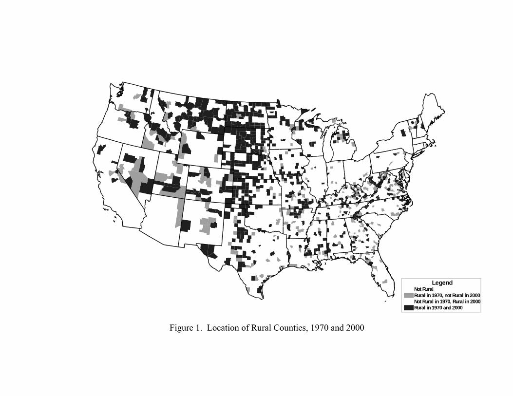
LegendNot RuralRural in 1970, not Rural in 2000Not Rural in 1970, Rural in 2000Rural in 1970 and 2000

Figure 1. Location of Rural Counties, 1970 and 2000

31

Appendix Table A1

Articles Addressing Metro/Nonmetro or Rural/Urban Differences Over Time: Published In Rural Sociology, Growth and Change, AJAE, Regional Studies & Journal of Regional Science, 2002-present

Article Data Time Frame Urban/Rural Classification Period Potential Biasa

Albrecht, D.E. and C.M. Albrecht, 2004. “Metro/Nonmetro Residence, Nonmarital conception and Conception Outcomes,” Rural Sociology 69(3), 430-452.

1995 Cycle of the National Survey of Family Growth

1965 -1995 1990 classifications E

Allen, B.L., 2002. “Race and Gender Inequality in Homeownership: Does Place Make a Difference?” Rural Sociology 67(4), 603-621.

IPUMS 1970, 1980, 1990

Unclear U

Barkley, D.L., M.S. Henry and S. Nair, 2006. “Regional Innovation Systems: Implications for Nonmetropolitan Areas and Workers in the South,” Growth and Change 37(2), 278-306.

Various 1990-2000 1990 classifications by Tolbert and Sizer (1996).

B

Braisier, K.J., 2005. “Spatial Analysis of Changes in the Number of Farms During the Farm Crisis,” Rural Sociology 70(4), 540-560.

Census of Agriculture, Census, various other

1982-1992 1990 E

Carruthers, J.I. and A. C. Vias, 2005. “Urban, Suburban, and Exurban Sprawl in the Rocky Mountain West: Evidence from Regional Adjustment Models,” Journal. of Regional Science 45(1), 21-48.

BEA, Census, CBP, various other

1982-1997 1990 classifications E

Goe, W. R., 2002. “Factors Associated with the Development of Nonmetropolitan Growth Nodes in Producer Services Industries, 1980-1990,” Rural Sociology 678(3), 416-441.

Economic Census, CBP

1980-1990 1990 classifications E

Goetz S .J. and Rupasingha A., 2002. “The New Rural Economy: High–Tech Firm Clustering: Implications for Rural Areas,” American Journal of Agricultural Economics 84(5)1229-1236.

CBP 1990-1999 Unclear U

Hammond, G. W. and E. Thompson, 2004. “Employment Risk in U.S. Metropolitan and Nonmetropolitan Regions: the Influence of Industrial Specialization and Population

BEA 1969-1999 Commuting regions based on 1990 classifications: Metropolitan regions include at least one (MSA) or (PMSA).

E

32

Characteristics,” Journal of Regional Science, 44(3), 517-542.

Nonmetropolitan regions do not include an MSA. 256 metro regions and 466 nonmetro regions in the lower 48 U.S. states.

Huang T-L., Orazem P.F and Wohlgemuth D., 2002. “Rural Population Growth, 1950–1990: The Roles of Human Capital, Industry Structure, and Government Policy,” American Journal of Agricultural Economics 84(3), 615-627.

Census, other various

1950-1990 Applied 1980 definitions and criteria to approximate 1950 classifications

B

Hunter, L. & J. Sutton, 2004. “Examining the Association Between Hazardous Waste Facilities and Rural ‘Brain Drain,’” Rural Sociology 69(2), 197-212.

US Census , 85-90 migration data

1985-1990 Unclear, 2358 NM counties implies the use of 1980 classifications

B

Hunter L. M., J. D. Boardman, and J. M. Saint Onge, 2005. “The Association Between Natural Amenities, Rural Population Growth, and Long-Term Residents’ Economic Well-Being,” Rural Sociology 70(4), 452-469.

Panel Study of income Dynamics, USDA, other various

1990-2001 Unclear U

Kwang-Koo, K., D.W. Marcouiller and S. Deller, 2005. “Natural Amenities and Rural Development: Understanding Spatial and Distributional Attributes,” Growth and Change 36(2), 273-297.

BEA, Census 1980-1990 Unclear U

Leichenko, R. and J. Silva, 2004. “International Trade, Employment and Earnings: Evidence from US Rural Counties,” Regional Studies 38(4), 355–374.

Census (LRD), other various

1972-1995 Unclear U

Martin, R. W., 2004. “Spatial Mismatch and the Structure of American Metropolitan Areas, 1970-2000,” Journal. of Regional Science 44(3), 467-488.

Census, CBP 1970-2000 2000 MSA designations (729 counties belonging to 179 MSAs)

E

McLaughlin, D., 2002. “Changing Income Inequality in Nonmetropolitan Counties, 1980 to 1990,” Rural Sociology 67(4), 512-533.

Census 1980-1990 Unclear, 2257 NM counties implies the use of 1990 classifications

E

Mills, B and G. Hazarika, 2003. “Do Single Mothers Face Greater Constraints to Work Force Participation in Nonmetropolitan Areas?” American Journal of Agricultural Economics, 85(1), 143-161.

CPS 1993-1999 Unclear U

Nelson, P.B., J.P. Nicholson, and E. H. Stege, 2004. “The Baby Boom and Nonmetropolitan Population Change,

PUMS (1980 and 1990 Censuses)

1975-1990 1980 B

33

1975-1990,” Growth and Change 35(4), 525-544. Pagoulatus, S., S. Goetz, D. Debertin, & T. Johannson, 2004. “Interactions Between Economic Growth and Environmental Quality in US Counties, 1987-1995,” Growth and Change 35(1), 90-108.

USA Counties 1987-1995 Unclear, 23% of counties designated as metro which implies the use of 1980 classifications

B

Renkow, M., 2003. “Employment Growth, Worker Mobility, and Rural Economic Development,” American Journal of Agricultural Economics 85(2), 503-513.

Census, BEA ’80-‘90 1980 classifications B

Sharp, J., B. Roe and E. Irwin, 2002. “The Changing Scale of Livestock Production in and around Corn Belt Metropolitan Areas, 1978–97,” Growth and Change 33(1), 115-132.

Ag Census, Census 1978-1997 1990 classifications E

Slack, T. & L. Jensen, 2002. “Race, Ethnicity and Underemployment in Nonmetropolitan America: A 30-Year Profile,” Rural Sociology 67(2), 208-237.

CPS 1968-1998 Unclear U

Snyder, A., S. Brown & E. Condo, 2004. “Residential Differences in Family Formation: The Significance of Cohabitation,” Rural Sociology 69(2), 235-260.

1995 Cycle of the National Survey of Family Growth

1965 -1995? (retrospective marital, fertility histories

1990 classifications E

Snyder A. and D. McLaughlin, 2004. “Female-Headed Families and Poverty in Rural America,” Rural Sociology 69(1), 127-149.

CPS 1980, 1990, 2000

Unclear U

Stretesky, P, J. Johnson and J. Arney, 2003. “Environmental Inequity: An Analysis of Large-Scale Hog Operations in 17 States, 1982-1997,” Rural Sociology 68(2), 231-252.

Ag Census 1982, 1987, 1992, 1997

1990 classifications E

Thomas, J. and F. Howell, 2003. “Metropolitan Proximity and US Agricultural Productivity 1978-1997,” Rural Sociology 68(3), 366-386.

Ag Census 1978, 1982, 1987, 1992, 1997

Use 1980 classifications for changes over the 1978-87 period and 1990 classifications for changes over the 1992-97 period

C

Vias, A.C. and J.I. Carruthers, 2005. “Regional Development and Land Use Change in the Rocky Mountain West, 1982-1997,”Growth and Change 36(2), 244-272

BEA, Census, CBP, various other

1982-1997 1990 classifications E

34

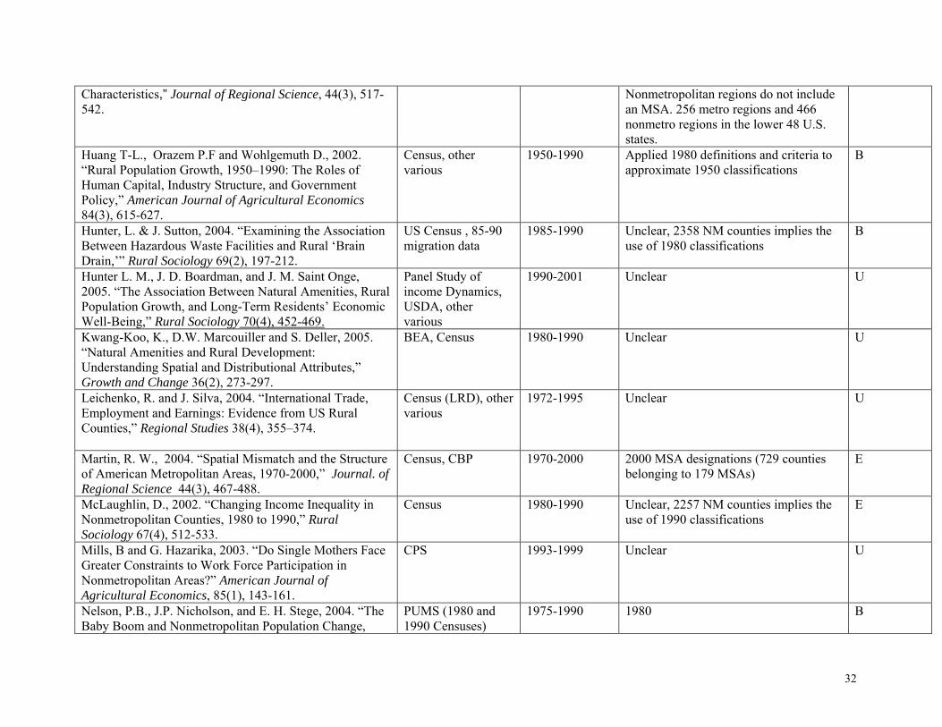
aPossible bias due to sample selection where B indicates classification of rural/urban or nonmetropolitan/metropolitan at the beginning of the analysis, E designates classification in the middle or at the end of the analysis, C means the authors allow the status to change over time and U indicates that the timing of classification is unknown.

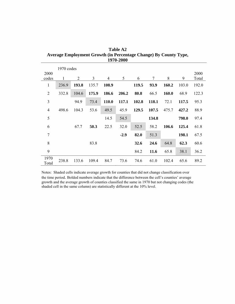
Table A2

Average Employment Growth (in Percentage Change) By County Type, 1970-2000

1970 codes

2000 codes 1 2 3 4 5 6 7 8 9

2000 Total

1 236.9 193.8 135.7 108.9 119.5 93.9 160.2 103.0 192.0

2 332.8 104.6 175.9 186.6 206.2 80.8 66.5 160.0 68.9 122.3

3 94.9 73.4 110.0 117.1 102.8 118.1 72.1 117.5 95.3

4 498.6 104.3 53.6 49.5 45.9 129.5 107.5 475.7 427.2 88.9

5 14.5 54.5 134.8 798.0 97.4

6 67.7 50.3 22.5 32.0 52.5 58.2 106.6 125.4 61.8

7 -2.9 82.0 51.3 198.1 67.5

8 83.8 32.6 24.6 64.8 62.3 60.6

9 84.2 11.6 65.8 38.1 36.2 1970 Total 238.8 133.6 109.4 84.7 73.6 74.6 61.0 102.4 65.6 89.2

Notes: Shaded cells indicate average growth for counties that did not change classification over the time period. Bolded numbers indicate that the difference between the cell’s counties’ average growth and the average growth of counties classified the same in 1970 but not changing codes (the shaded cell in the same column) are statistically different at the 10% level.

36

Table A3 Average Real Income Growth (in Percentage Change) By County Type,

1970-2000

1970 codes 2000 codes 1 2 3 4 5 6 7 8 9

2000 Total

1 307.2 284.8 190.9 217.8 231.8 159.4 300.8 195.7 282.3

2 377.7 148.0 276.9 316.0 382.0 172.5 141.8 296.3 156.9 197.7

3 129.8 115.4 156.6 164.8 173.8 167.4 156.0 233.4 150.9

4 895.4 161.2 106.3 90.6 84.4 211.5 162.3 294.3 771.3 144.8

5 31.5 82.3 165.8 944.9 128.4

6 97.5 90.3 56.5 73.6 100.1 114.7 167.7 199.3 114.4

7 28.4 122.8 81.8 251.3 100.7

8 101.5 77.3 77.8 115.7 114.9 112.0

9 118.0 38.9 155.0 74.1 71.6 1970 Total 310.8 192.9 171.6 140.8 113.0 138.7 101.0 181.8 112.4 143.7

Notes: Shaded cells indicate average growth for counties that did not change classification over the time period. Bolded numbers indicate that the difference between the cell’s counties’ average growth and the average growth of counties classified the same in 1970 but not changing codes (the shaded cell in the same column) are statistically different at the 10% level.

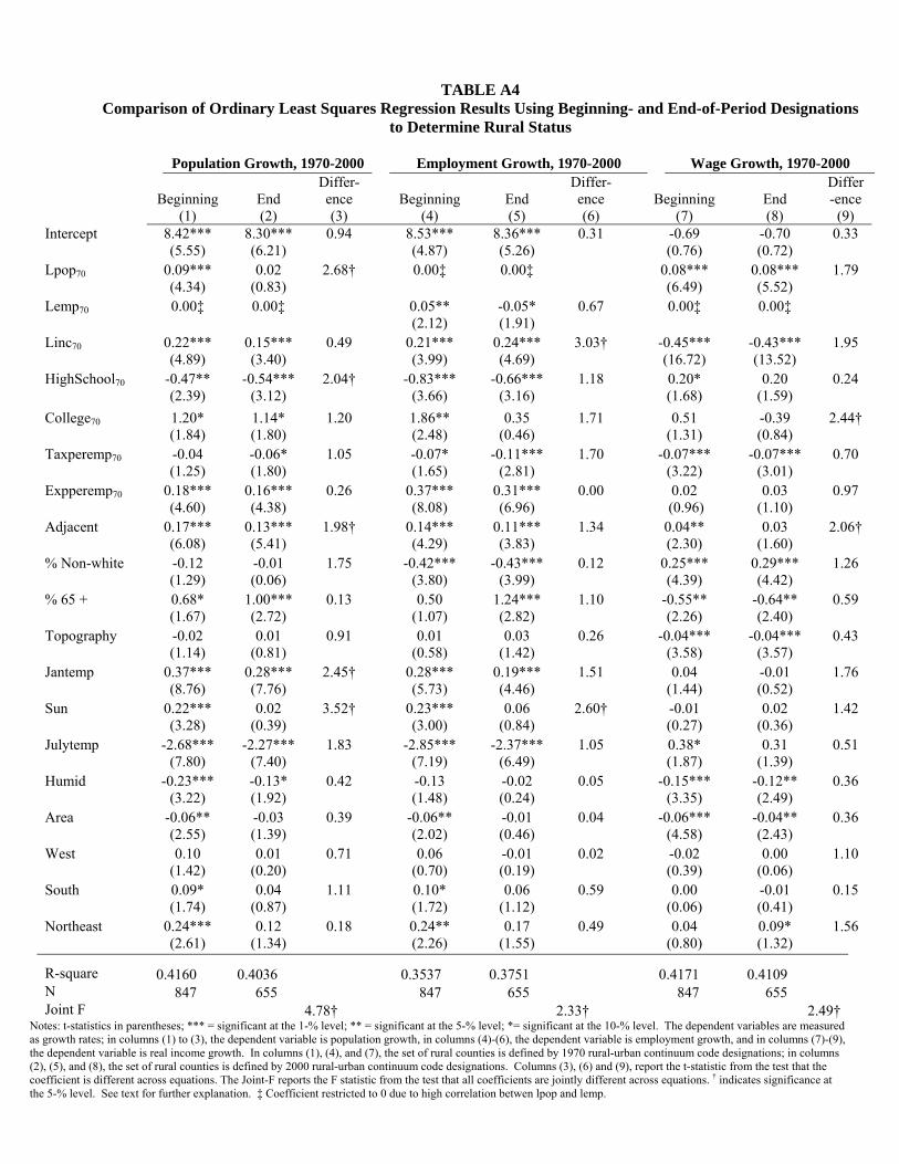
TABLE A4

Comparison of Ordinary Least Squares Regression Results Using Beginning- and End-of-Period Designations to Determine Rural Status

Population Growth, 1970-2000 Employment Growth, 1970-2000 Wage Growth, 1970-2000

Beginning

(1) End (2)

Differ-ence (3)

Beginning (4)

End (5)

Differ-ence (6)

Beginning (7)

End (8)

Differ-ence

(9) Intercept 8.42***

(5.55) 8.30*** (6.21)

0.94 8.53*** (4.87)

8.36*** (5.26)

0.31 -0.69 (0.76)

-0.70 (0.72)

0.33

Lpop70 0.09*** (4.34)

0.02 (0.83)

2.68† 0.00‡ 0.00‡ 0.08*** (6.49)

0.08*** (5.52)

1.79

Lemp70 0.00‡ 0.00‡ 0.05** (2.12)

-0.05* (1.91)

0.67 0.00‡ 0.00‡

Linc70 0.22*** (4.89)

0.15*** (3.40)

0.49 0.21*** (3.99)

0.24*** (4.69)

3.03† -0.45*** (16.72)

-0.43*** (13.52)

1.95

HighSchool70 -0.47** (2.39)

-0.54*** (3.12)

2.04† -0.83*** (3.66)

-0.66*** (3.16)

1.18 0.20* (1.68)

0.20 (1.59)

0.24

College70 1.20* (1.84)

1.14* (1.80)

1.20 1.86** (2.48)

0.35 (0.46)

1.71 0.51 (1.31)

-0.39 (0.84)

2.44†

Taxperemp70 -0.04 (1.25)

-0.06* (1.80)

1.05 -0.07* (1.65)

-0.11*** (2.81)

1.70 -0.07*** (3.22)

-0.07*** (3.01)

0.70

Expperemp70 0.18*** (4.60)

0.16*** (4.38)

0.26 0.37*** (8.08)

0.31*** (6.96)

0.00 0.02 (0.96)

0.03 (1.10)

0.97

Adjacent 0.17*** (6.08)

0.13*** (5.41)

1.98† 0.14*** (4.29)

0.11*** (3.83)

1.34 0.04** (2.30)

0.03 (1.60)

2.06†

% Non-white -0.12 (1.29)

-0.01 (0.06)

1.75 -0.42*** (3.80)

-0.43*** (3.99)

0.12 0.25*** (4.39)

0.29*** (4.42)

1.26

% 65 + 0.68* (1.67)

1.00*** (2.72)

0.13 0.50 (1.07)

1.24*** (2.82)

1.10 -0.55** (2.26)

-0.64** (2.40)

0.59

Topography -0.02 (1.14)

0.01 (0.81)

0.91 0.01 (0.58)

0.03 (1.42)

0.26 -0.04*** (3.58)

-0.04*** (3.57)

0.43

Jantemp 0.37*** (8.76)

0.28*** (7.76)

2.45† 0.28*** (5.73)

0.19*** (4.46)

1.51 0.04 (1.44)

-0.01 (0.52)

1.76

Sun 0.22*** (3.28)

0.02 (0.39)

3.52† 0.23*** (3.00)

0.06 (0.84)

2.60† -0.01 (0.27)

0.02 (0.36)

1.42

Julytemp -2.68*** (7.80)

-2.27*** (7.40)

1.83 -2.85*** (7.19)

-2.37*** (6.49)

1.05 0.38* (1.87)

0.31 (1.39)

0.51

Humid -0.23*** (3.22)

-0.13* (1.92)

0.42 -0.13 (1.48)

-0.02 (0.24)

0.05 -0.15*** (3.35)

-0.12** (2.49)

0.36

Area -0.06** (2.55)

-0.03 (1.39)

0.39 -0.06** (2.02)

-0.01 (0.46)

0.04 -0.06*** (4.58)

-0.04** (2.43)

0.36

West 0.10 (1.42)

0.01 (0.20)

0.71 0.06 (0.70)

-0.01 (0.19)

0.02 -0.02 (0.39)

0.00 (0.06)

1.10

South 0.09* (1.74)

0.04 (0.87)

1.11 0.10* (1.72)

0.06 (1.12)

0.59 0.00 (0.06)

-0.01 (0.41)

0.15

Northeast 0.24*** (2.61)

0.12 (1.34)

0.18 0.24** (2.26)

0.17 (1.55)

0.49 0.04 (0.80)

0.09* (1.32)

1.56

R-square 0.4160 0.4036 0.3537 0.3751 0.4171 0.4109 N 847 655 847 655 847 655 Joint F 4.78† 2.33† 2.49†

Notes: t-statistics in parentheses; *** = significant at the 1-% level; ** = significant at the 5-% level; *= significant at the 10-% level. The dependent variables are measured as growth rates; in columns (1) to (3), the dependent variable is population growth, in columns (4)-(6), the dependent variable is employment growth, and in columns (7)-(9), the dependent variable is real income growth. In columns (1), (4), and (7), the set of rural counties is defined by 1970 rural-urban continuum code designations; in columns (2), (5), and (8), the set of rural counties is defined by 2000 rural-urban continuum code designations. Columns (3), (6) and (9), report the t-statistic from the test that the coefficient is different across equations. The Joint-F reports the F statistic from the test that all coefficients are jointly different across equations. † indicates significance at the 5-% level. See text for further explanation. ‡ Coefficient restricted to 0 due to high correlation betwen lpop and lemp.