University of California, Berkeley

Undergraduate Senior Thesis

Reexamining Ferguson: The

effect of police officers on arrests

by raceAuthor:

Bhargav Gopal

Advisor:

Justin McCrary

May 6, 2015

1 Introduction

The shooting of Michael Brown in August of 2014 and the subsequent protests in

Ferguson, Missouri brought a sharp spotlight to the issue of race and policing in

the United States. The events prompted an investigation of the Ferguson Police

Department by the Department of Justice, and a report was issued in March of

2015 [1]. According to the report, of all arrests after car stops from 2012 to 2014,

93% of those arrests were of African American individuals. Furthermore, at the

time of the Michael Brown shooting, only 6% of the Ferguson police department

was black. Hence the ratio between percent black (white) arrests and percent black

(white) officers, which I will refer to as black (white) ratio, is 15.5.

The figures from Ferguson motivate the following research questions that I

answer in this paper: 1) is the black ratio ratio in Ferguson (15.5) atypical of the

US as a whole; 2) how have the black and white ratios changed over time; and

3) What is the effect of adding a black, white, or Asian officer on black, white,

or Asian arrests. Aggregated over all years in my dataset, I find that the white

ratio for every state in the US is less than 1, while the black ratio for every state is

greater than 1 (the only exception is New Mexico). A plausible explanation for why

African Americans are more represented in the arrested population as opposed to

the police population is that disadvantaged groups are hurt by the discretionary

process of defining and responding to criminal conduct[5, 6]. Another theory

is that the ratios do not indicate racial discrimination, but rather differences in

ability to enter the police force and differences in rates of offending[3]. In addition,

systematic discrimination where police forces hire whites at disproportionate rates,

and where white police officers discriminatorily arrest black suspects would also

be consistent with the ratios observed.

In this paper, I also use OLS to answer the following question: What is the

effect of adding a black, white, or Asian officer on black, white, or Asian arrests?

Notable theories regarding the effect of officers on crime include the Deterrence

and Incapacitation theories. The Deterrence theory states that criminal activity

becomes less attractive as the probability of arrest increases; the Incapacitation

theory states that adding police officers will eventually reduce criminal activity by

1

arresting the most prolific offenders[2]. While both theories suggest that adding

police officers reduces crime, the Deterrence theory implies that adding police

officers would reduce arrests, while the Incarceration theory implies that adding

police officers would initially increase arrests.

The Impact of Race on Policing and Arrests looks at a similar research question,

and the authors find that increases in the number of minority police are associated

with significant increases in arrests of whites but have little impact on arrests

of nonwhites[8]. They also argue that more white police increase the number of

arrests of nonwhites but do not systematically affect the number of white arrests.

While this paper examines a similar question, the effect of adding a black, white,

or Asian police officer on each of black, white, and Asian arrests, there are some

notable differences in the methodologies used between this paper and The Impact

of Race on Policing and Arrests.

First, the data that I use to examine the racial composition of municipal police

departments comes from the Law Enforcement Management and Administrative

Statistics (LEMAS), while the racial data on municipal police departments used in

The Impact of Race on Policing and Arrests comes from EEOC tabulations. In the

LEMAS dataset, we are able to see the number of full-time sworn officers by race.

In the EEOC, the figures represent officers whose job function is protective services,

which can include both sworn and unsworn police officers. Another difference

between this paper and The Impact of Race on Policing and Arrests is the fact

that in my paper, I do not divide my race categories into white and non-white.

Instead, I have arrest and officer figures for blacks, whites, and Asians. Finally,

another unique feature of my paper is the examination of the black, white, and

Asian ratio both over time and across different states in the US.

I use agency and year fixed effects, as well as 1987 Population weights when

implementing my regressions. Over various regression specifications, my dependent

variable is either the sum of black, white, and Asian arrests in a given agency and

year or the yearly sum of the number of arrests of a particulate race in a given

agency and year. The three independent variables are the counts of the number

of white, black, and Asian officers in a given agency and year. On the surface, the

2

model immediately suffers from 1) Omitted variable bias 2) Simultaneity bias, and

3) Measurement Error. Indeed, the possibility that the level of officers is partly

determined by the level of arrests has led to the creative use of instrumental

variables to measure the effect of officers on crime[9, 7]. In addition, if the level of

officers is correlated with potential omitted variables such as the local economy and

city budgets, the coefficients on the officer variables would be biased. Thus I rely

upon the fact that year over year changes in police have generally weak associations

with potential omitted variables such as the local economy, city budgets, social

disorganization, and recent changes in crime, suggesting that the Omitted Variable

and Simultaneity biases are not particularly worrisome. Since the arrest data

received from the Uniform Crime Reports (UCR) has measurement error, which

stems from factors such as differences in police department reporting practices

across jurisdictions, technological changes in crime reporting, and changes in crime

reporting by victims over time, the coefficients on the officer variables will be biased

downward[4].

The use of agency fixed effects is critical in obtaining an unbiased estimate of

the effect of adding an officer on the number of arrests. If agency fixed effects were

not included, increases in the number of officers could be correlated with unob-

served omitted variables that vary over different agencies. For example, it is not out

of the realm of possibility to imagine a world where agencies representing regions

with poor socio-economic characteristics have more officers and arrests. Thus, if

we do not include agency-fixed effects, we will most likely overstate the effect of

adding officers on the number of arrests. Similarly, population weights are neces-

sary for understanding the true relationship between officers and arrests. Since the

data is presented at the agency level, there are simply more agencies representing

small populations than large populations. Without population weights, we would

give, for example, equal weight to New York Police Department as Abbeville Police

Department. However, we know that New York Police Department represents a

population much larger than Abbeville Police Department, and we can give more

weight to agencies that represent larger populations.

3

2 Data

The FBI’s Uniform Crime Reports (UCR) provides information regarding the num-

ber of arrests, broken down by race, undertaken by agencies across the United

States in a given year. The UCR data is available annually from 1980 until 2012,

and I access agency level data where arrests are organized by age, sex, and race.

The relevant variables I access in the UCR data are adult white arrests, adult

black arrests, adult Asian arrests, originating reporting agency identifier (ORI),

agency name, and state. The ORI code uniquely identifies a police agency. Since

the arrest data within a given year are reported monthly, for each agency, I sum

arrests for all months to find the total yearly arrests undertaken by a given agency.

The Law Enforcement Management and Administrative Statistics (LEMAS)

provides agency level information regarding the organization and administration

of police and sheriff departments that employ 100 or more full time sworn officers.

Information about a nationally representative sample of smaller agencies is also

included. The LEMAS years that I access are 1987, 1990, 1993, 1997, 2000, and

2007. The 1999 LEMAS dataset is a limited version that doesn’t contain the race

variables for police officers. The relevant LEMAS variables that I access are full

time sworn white officers, full time sworn black officers, full time sworn Asian

officers, agency name, state, and ORI (if available).

To ultimately construct my final dataset, I merged the officer race information

provided by LEMAS and the arrest race information provided by the UCR. For

the years where the ORI code was included in both LEMAS and UCR, I merged

using the ORI code as the unique identifier. When the ORI code was not available

for both datasets, I merged based on agency name and state.

After the LEMAS and UCR information is merged together for the available

years, there are 7847 total observations. Of the 7847 observations, there are 4293

unique agencies. Table 1 presents the number of observations in each year. There

are fewer observations in 1987 due to difficulties in finding a common identifier

between the LEMAS and UCR data. Table 2 presents the weighted means for

the number of white, black, and Asian arrests or officers in a given agency. Since

there are significant differences in the sizes of different agencies (measured by the

4

size of the population an agency represents), weights proportional to the size of

the population an agency represents are used. If weights are not used, we will

overestimate statistics and features from the smaller agencies. I follow convention

by using population weights that are measured in a particular year (I use 1987

population, which is the first year that I consider in my analysis). Table 3 shows

that half the agencies represent a population that is less than 15,560. Naturally,

half the agencies represent populations more than 15,560, but some agencies in

the dataset are particularly large. In fact, there are 9 agencies in the dataset that

represent 1987 populations greater than 1,000,000.

2.1 Data shortcomings

An important omission from my data is Hispanic arrest and race information. The

reason Hispanic information is not included is because the UCR does not have

any information about Hispanic arrests except in 2013[10]. The FBI discontinued

collecting ethnic based crime data in 1987 (only to reinstate in 2013), and as a

result, the Hispanic figures are implicitly part of white arrests and white officers.

If the Hispanic information were available and if the ratio of Hispanic arrests to

Hispanic officers were greater than the ratio of white arrests to white officers, then

the current statistic of white officer/white arrest overstates the true ratio.

The fact that an agency voluntarily submits reports on crimes also presents an

issue. Agencies have the option of simply not reporting UCR data in a given year.

As a result, many agencies are only observed in 1 year. The fact that a sizable

number of agencies are only observed in 1 year reduces the relevant sample size

when performing a demeaned regression. In addition, even if an agency does file

UCR reports in a given year, the data have measurement error problems. The

issue of agencies self-reporting statistics is also partially present in the LEMAS

data. Large agencies with 100 or more full time sworn officers self report, while

the smaller law enforcement agencies chosen through a stratified random sample

were not allowed to self-report.

The exclusion of a host of covariates in the regression specification presents a

concern if one is worried about omitted variable bias. Namely one could worry

5

that even within an agency, an outside variable such as the local economy could

influence both officer and arrest levels. While the inclusion of potential covariates

would be ideal, I rely upon evidence that year over year changes in police levels

are uncorrelated with the local economy, city budgets, social disorganization, and

recent changes in crime[4].

Finally, the lack of a common identifier that is consistent in both the UCR and

LEMAS data over all years presents difficulties in matching arrest data to police

data. If such an identifier existed, my sample size would be larger, and there would

be more agencies that are observed in multiple years.

3 Methodology

The primary statistic I use to compare a race’s representation in the police force to

representation in the arrest population is the race ratio := % race arrested/% race officers.

If, for the sake of example, an agency has 100 officers, 10 black officers, 500 arrests,

and 400 black arrests, then the black ratio = .8/.1 = 8. A competing statistic that I

elect not to use is the race difference:=% race arrests - % race officers. Empirically,

if we compare the black difference statistic across states, we find that the black

difference is inflated in states with large black populations. A strength of the race

difference statistic that is not present in the race ratio statistic is that one can

calculate the race difference statistic for every agency. When the denominator of

the race ratio statistic is 0 (when there are 0 officers of a certain race), then we

cannot calculate the race ratio statistic.

Figure 1 shows the weighted and un-weighted means of the race ratio statistic

for blacks, whites, and Asians. Since the race ratio statistic cannot be calculated

for agencies with 0 officers of a given race, I define the mean of race.ratio, race.ratio

= (%race.arrested)

(%race.officers). Analogously, the weighted mean of race.ratio = weighted mean

(% race arrested) / weighted mean (% race officers), where the weights are provided

by the size of the population an agency represents in 1987. Hence after canceling

terms, the equation for the weighted mean ratio is the following, where the unit

of analysis is the agency:

6

n∑i=1

(popi)(percent.racei)

n∑i=1

(popi)(percent.officeri)

Figure 2 shows how the weighted mean ratio for blacks, whites, and Asians have

changed since 1990. Only agencies observed over all years are tracked. Hence the

time series shows how the weighted mean ratio has changed for the same basket

of agencies over time. Tracking the same agencies over time is important because

in any given year, agencies might self-select to report their arrest or officer figures.

A caveat of interpreting the figure is that the agencies that do appear in all the

years tend to be larger agencies. The reason 1987 is not included is because there

are relatively fewer observations in 1987 than in other years, as shown in Table 1.

Thus, if 1987 were included, the number of agencies that we observe over all years

in the data dwindles. In addition, the means for each year are weighted to give

greater weight to agencies that represent larger populations.

Figures 3 and 4 show the weighted mean ratio for blacks and whites within

each state. Thus for each state separately, I calculate the weighted mean using the

weighted mean ratio formula presented earlier.

3.1 Regression Specification

I estimate models of two forms. The first form is as follows:√race.arrestsit =B0+

√white.officersit∗B1+

√black.officersit∗B2+

√Asian.officersit∗

B3 +D ∗ γ + T ∗ φ+ εit

The second form is as follows:

log√BWA.arrestsit = B0 + logB1 ∗

√BWA.officers+ +D ∗ γ + T ∗ φ+ εit

The unit of observation is at the agency-time level. In the first form, the

dependent variable is the number of arrests of a certain race. The X matrix

contains the level of black officers, white officers, and Asian officers. The T matrix

consists of dummies for each year in the dataset (except the first year). The D

matrix consists of dummies for each agency in the dataset (except the first agency).

In the second form, the dependent variable is the sum of black, white, and Asian

arrests in a given agency-year. The independent variable is the sum of black,

white, and Asian officers in a given agency-year. ε represents the error term in

7

both forms. Both forms also are weighted by the 1987 population. 1

The use of agency fixed effects in both forms is very important in obtaining

an unbiased estimate of the effect of adding an officer on the number of arrests.

Suppose, for example, that a city’s collective consciousness about crime is unob-

served and influences both the officer counts and the number of arrests in a given

agency. Also suppose that this unobserved variable is constant within a city but

varies between cities. Then if agency fixed effects are not included, we will obtain

an unbiased estimate. 2

In the second form, the B1 term represents the elasticity of BWA.arrests with

respect to BWA.officers. Since the dataset only includes agencies that have total

arrest counts and total officer counts greater than 0, the independent and de-

pendent variable are finite under the log transformation. Hence the coefficient

represents an elasticity: a 1% increase in BWA.officers is associated with a β̂1%

increase in BWA.arrests. Also, the standard error of the elasticity is simply the

standard error of β̂1

In the first form, we cannot report to taking logs of the dependent and inde-

pendent variables without throwing observations away. The reason is that many

agencies have 0 officers of a particular race (such as 0 Asian officers). Taking the

log of a variable with 0 as a value would yield −∞, and would consequently bias

our estimate of the elasticity. Instead, we apply a square root transformation to

the data, and calculate the elasticity of race.arrests with respect to race.officers in

the following way:

εy,x =√xi/√yi ∗ β̂

SE(εy,x) =√xi/√yi ∗ SE(β̂)

Here the averages are weighted averages, where the weights are determined by

the 1987 population. Furthermore, β̂ refers to coefficient on x when y is regressed

1In both forms, the coefficients are achieved through demeaning, rather than including dum-mies for every agency. In addition, due to large variation in the size of various police forces inthe dataset, transformations that pull down extreme values (ie. sqrt and log) are used to preventthe regression coefficients from being unduly influenced by extreme values.

2Year fixed effects are also important in controlling for omitted variables that vary over timebut not over agency.

8

on x and other independent variables. Note that for some agencies, yit, the number

of arrests of a certain race in a given year, is 0. Thus when calculating the elasticity,

we calculate the weighted average of the numerator and denominator separately.

4 Results

4.1 Graphical Results

Figure 1 compares the weighted and unweighted means of the ratio statistic for

blacks, whites, and Asians. In both the weighted and unweighted cases, the ratio

for whites and Asians is less than or equal to 1, while the ratio for blacks is above

1. Hence, on average, the proportion of all arrests that are white or Asian is less

than the proportion of all officers that are white or Asian. Conversely, the the

proportion of all arrests that are black is greater than the proportion of all officers

that are black by a factor of at least 2.5. Notice that when weighted averages

are calculated by using population weights, the weighted mean ratio is less than

the unweighted mean ratio for all races. The fraction of all arrests that are white

decreases from .78 to .66 when we take into account population weights. The

fraction of all officers that are white decreases from .93 to .86 when population

weights are used. The results imply that in areas with larger populations, agencies

have a smaller fraction of white officers and white arrests relative to the average

agency in the dataset. On the other hand, the proportion of all arrests that are

black increases from .21 to .32 when we use a weighted mean. The fraction of

all officers that are black increases from .06 to .11 when we take into account

the population weights. The results imply that in areas with larger populations,

agencies have a larger fraction of black officers and black arrests relative to the

average agency in the dataset. The change when we use population weights is

greatest for Asians. The mean fraction of Asian arrests doubles from .005 to .01,

while the mean fraction of Asian officers quadruples from .005 to .02. The results

imply that in areas with larger populations, agencies have a larger fraction of Asian

officers and Asian arrests relative to the average agency in the dataset.

Figure 2 shows how the weighted mean ratio for blacks, whites, and Asians

9

have changed since 1990 for agencies we observe in all years. As can be readily

seen, the weighted mean ratio has been monotonically decreasing for blacks and

has been monotonically increasing for whites. The ratio for Asians is lower in 2007

than the ratio in 1990; however, for all observed years before 2007, the ratio has

been monotonically increasing. For each race, a paired difference t-test can be

used to examine if the difference between the 2007 and 1990 ratio is significantly

different from 0. I find that the t statistic for whites, blacks, and Asians is 3.09,

-2.65, and -3.03 respectively. Hence for all races, the ratios in 2007 are significantly

different from the ratios in 2000 at the 5% level. The formula used to calculate

the t-statistic for a particular race is in the footnotes. 3

Figures 3 and 4 show the weighted mean ratio for blacks and whites within

each state over all years. From Figure 3, we see that the weighted white ratio

is smallest in the southeastern states of the US. From Figure 4, we see that the

weighted black ratio is typically larger for states in the north and north-east. Far

west states tend to have lower black ratios and higher black ratios relative to other

states.

4.2 Regression Results and Elasticities

We are interested in finding the effect of adding a police officer on arrested made by

police officers, and figure 5 shows the general relationship between police officers

and arrests. Quite unsurprisingly, we see that more total officers, which is referred

to in this paper as BWA officers, is associated with more total arrests, denoted as

BWA arrests. The scatterplot also compares the relationship between officers and

arrests for each year available by fitting a separate line of best fit for each year.

The slopes of the lines for each year is obtained by fitting a regression of total

officers on total arrests and an interaction term between total arrests and year.

As the visual analysis confirms, the effect of officers on arrests is stronger in 1987

3paired difference t stat = ∆ratio√√√√ N∑i=1

(∆ratioi−∆ratio)2/N

, where we take a weighted mean of the

∆ ratio, and N refers to the number of agencies that have a difference in ratio that is finite.

10

than it is in any other year 4. While figure 5 demonstrates the general relationship

between officers and arrests, the slopes overstate the impact of officers on arrests

because the slopes are the product of a pooled regression. In effect, an increase

in police officers might be associated with towns that have poorer socioeconomic

standings, which could be associated with more arrests. To find a more accurate

estimate of the effect of adding a police officer on arrests, we need to use the within

estimator, and we also need to see how the effect of adding an officer on arrests

depends on the race of the officer and the race of the arrestee.

The results obtained in tables 6 through table 9 are all products of regressions

where agency fixed effects, time fixed effects, and population weights are used.

Thus the coefficients can approximately be interpreted as the average effect of

X on Y within each agency. We are primarily interested in the coefficients from

tables 6 through 9 as a means of calculating the elasticity between arrests of a

certain race and officers of a certain race 5. However, the coefficients on the year

dummies in these tables do carry some valuable information. The square root of

black and white arrests has decreased significantly6 from 1987 to 2007, while the

square root of Asian arrests has increased during the same time period.

The most important numerical results in this paper are found in table 5, which

represents the elasticities of arrests with respect to officers by race. The elasticity

in the second row, for example, can be interpreted as follows: ”At the weighted

mean of white arrests and white officers, a 1% increase in white officers is associated

with a .38% increase in white arrests.” There are a couple important facts to note.

First, for all races, the elasticity of arrests with respect to white officers is greater

than the elasticity with respect to black and Asian officers. If we treat these results

as causal estimates, the figures imply that on average, white officers arrest suspects

of all races more frequently than black or Asian officers. Second, we observe that

an officer is most likely to arrest an individual of his or her own race. The elasticity

of arrests with respect to white officers is greatest for white arrests; the elasticity

4In fact, the slope in 1987 is significantly larger than the slope in any other year at the 5%level, except for 2007

5Recall the equation to calculate the elasticity using a square root transformation in page 76at the 5% level

11

of arrests with respect to black officers is greatest for black arrests; the elasticity

of arrests with respect to Asian officers is greatest for Asian arrests. The third

important fact is that on average, a 1% increase in police officers is associated

with a .138% increase in arrests for all levels of officers and arrests7. Finally,

we should notice that the estimates of the elasticity standard errors are smallest

when measuring the elasticity of arrests with respect to Asian officers. However,

the t-statistics are largest for the elasticities with respect to white officers.

5 Conclusion

This paper sets out to answer the following questions: 1) is the black ratio ratio in

Ferguson (15.5) in 2014 atypical of the US as a whole; 2) how have the black, white,

and Asian ratios changed over time; and 3) What is the effect of adding a black,

white, or Asian officer on black, white, or Asian arrests. Of the 3891 observations

of agency-pairs that have a finite black ratio, only 133 observations have a black

ratio above 15.5. Thus Ferguson’s black ratio in 2014 would place itself in the

top 5%. Of the 169 observations in Missouri, only 3 agency-time observations

have a black ratio above 15.5. In addition, table 4 shows that 23 states have 0

agencies that had a black ratio above 15.5 at any year observed in the dataset.

Thus, by these measures, Ferguson’s black ratio is atypical of the US’ black ratio.

The weighted black ratio has been steadily declining in every year observed in the

dataset (As seen in Figure 2). However, in each year, the weighted black ratio

is still greater than 1. The weighted white ratio has been fairly constant over all

years at a value below 1. The Asian ratio has also been fairly constant over all

years at a value below 1, although we observe a decline in 2007. Finally, we see

that white officers arrest suspects of all races more frequently than black or Asian

officers, and that an officer is most likely to arrest an individual of his or her own

race. Further research could examine why an officer is more likely to arrest an

individual of the same race.

7This is true because the coefficient from a log-log regression represents elasticity

12

References

[1] Investigation of the Ferguson Police Department, 2015

[2] Berk, Richard and Lawrence A. Sherman, The specific deterrent effects of arrest

for domestic assault,1984

[3] Blumstein, Alfred, On the racial disproportionality of United States’ prison

populations, 1982

[4] Chalfin, Aaron and Justin McCrary, The Effect of Police on Crime: New Evi-

dence from US Cities, 1960-2010, 2012

[5] Chambliss, William Crime and the legal process, 1969

[6] Davidson, Laura, Douglas Smith, and Christy A. Visher, Equity and discre-

tionary justice: The influence of race on police arrest decisions, 1984

[7] Di Tella, Rafael and Ernesto Schargrodsky Do police reduce crime? Estimates

using the allocation of police forces after a terrorist attack, 2004

[8] Donohue, John and Steven Levitt, The Impact of Race on Policing and Arrests,

2001

[9] Levitt, Steven, Levitt, Using electoral cycles in police hiring to estimate the

effect of police on crime, 1997

[10] Planas, Roque. ”FBI To Track Latino Arrests For Uniform Crime Report.”

The Huffington Post

13

Table 1: means weighted by population

weighted average over all agencies

white.officers 1, 020.127black.officers 298.697Asian.officers 41.057white.arrests 14, 582.440black.arrests 13, 186.450Asian.arrests 352.901BWA.officers 1, 359.881BWA.arrests 28, 121.790

Table 2: Distribution of size of agencies

Q1 Q2 Q3 Q4

pop.quartiles 91 - 5156 5157 - 15560 15561 - 54530 54531 - 3,870,000number.of.agencies 1367 1222 1048 658

Table 3: Number of observations by year

years obs.by.year

1 1987 4302 1990 1, 6063 1993 1, 5154 1997 1, 6245 2000 1, 5536 2007 1, 119

14

Table 4: Statistics by state

State Percent observations with black ratio above ferguson’s Number of observations

34 NY 14.516 12439 RI 13.462 5222 MI 8.215 3537 CT 5.814 17231 NJ 3.491 40120 MD 2.941 6823 MN 2.765 21741 SD 2.128 473 AR 2.041 14727 NC 1.792 27924 MO 1.775 16944 UT 1.754 5738 PA 1.592 37721 ME 1.408 7116 KS 1.389 7214 IL 1.351 14825 MS 1.235 816 CO 1.136 17648 WI 1.111 18012 IA 1.075 18643 TX 1.043 67149 WV 0.962 10435 OH 0.913 21936 OK 0.885 2262 AL 0.515 1945 CA 0.462 64910 GA 0.342 2921 AK 0.000 164 AZ 0.000 1118 DE 0.000 339 FL 0.000 14911 HI 0.000 913 ID 0.000 6315 IN 0.000 15217 KY 0.000 7918 LA 0.000 11619 MA 0.000 20826 MT 0.000 2728 ND 0.000 5129 NE 0.000 6130 NH 0.000 6432 NM 0.000 4433 NV 0.000 1937 OR 0.000 13140 SC 0.000 17142 TN 0.000 22245 VA 0.000 18346 VT 0.000 1747 WA 0.000 14150 WY 0.000 48

15

Table 5: Elasticities of Arrests with Respect to Officers

comparison value standard.error

1 BWA arrests;BWA officers 0.138 0.0372 white arrests;white officers 0.380 0.0923 white arrests;black officers 0.092 0.1474 white arrests; Asian officers -0.009 0.0345 black arrests;white officers 0.335 0.1096 black arrests; black officers 0.150 0.1827 black arrests; Asian officers 0.051 0.0478 Asian arrests;white officers 0.233 0.1259 Asian arrests; black officers 0.098 0.14810 Asian arrests; Asian officers 0.059 0.037

Table 6: Regression of Total Arrests on Total Officers

Variable Coefficient (Std. Err.)lnBWAofficers 0.138 (0.037)1987 0.000 (0.000)1990 0.147 (0.050)1993 0.079 (0.045)1997 0.150 (0.044)2000 0.088 (0.048)2007 -0.035 (0.067)Intercept 8.109 (0.200)

Table 7: Regression of white Arrests on Officers using sqrt transformation

Variable Coefficient (Std. Err.)√white.officers 1.492 (0.361)√black.officers 0.863 (1.379)√Asian.officers -0.268 (1.010)

1987 0.000 (0.000)1990 0.320 (3.512)1993 -4.592 (3.874)1997 -3.300 (5.159)2000 -5.353 (4.210)2007 -11.965 (5.452)Intercept 55.602 (12.462)

Table 8: Regression of black Arrests on Officers using sqrt transformation

Variable Coefficient (Std. Err.)√white.officers 1.065 (0.347)√black.officers 1.135 (1.379)√Asian.officers 1.240 (1.147)

1987 0.000 (0.000)1990 1.704 (2.068)1993 0.375 (2.454)1997 -1.994 (3.423)2000 -3.197 (2.632)2007 -9.116 (4.171)Intercept 37.852 (9.564)

16

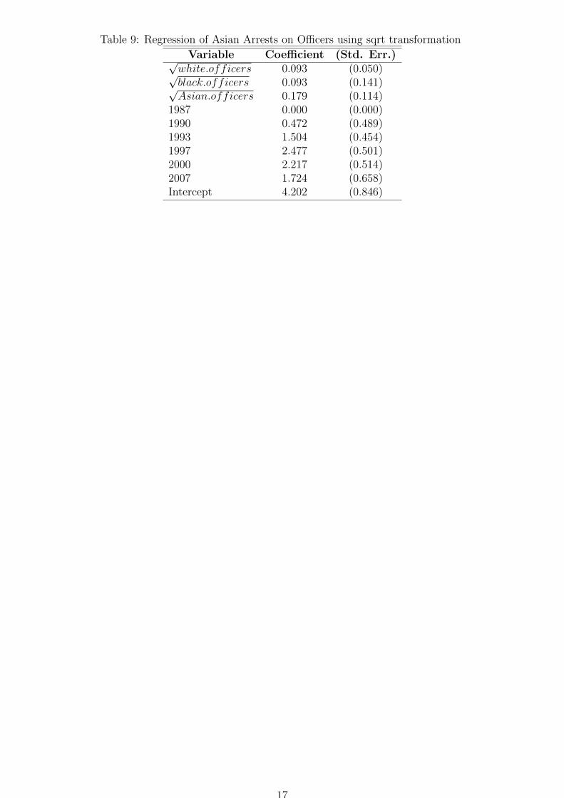
Table 9: Regression of Asian Arrests on Officers using sqrt transformation

Variable Coefficient (Std. Err.)√white.officers 0.093 (0.050)√black.officers 0.093 (0.141)√Asian.officers 0.179 (0.114)

1987 0.000 (0.000)1990 0.472 (0.489)1993 1.504 (0.454)1997 2.477 (0.501)2000 2.217 (0.514)2007 1.724 (0.658)Intercept 4.202 (0.846)

17

Weighted white white Weighted black black Weighted asian asian

Ratio between % race arrests and % race officersm

ean(

% r

ace

arre

sts)

/mea

n(%

rac

e of

ficer

s)

01

23

4

Figure 1

01

23

4Changes in ratio of %arrests to %officers over time

Year

mea

n %

arr

ests

/ mea

n %

offi

cers

{w

eigh

ted}

white ratioblack ratioasian ratio

1990 1993 1997 2000 2007

Figure 2

0.66

0.970.75

0.93

0.97

0.8

0.62

0.71

0.62

0.99

0.85 0.87

0.94

0.940.94

0.51

0.98

0.67

0.930.84

0.91

0.58

0.82

0.95

0.97

0.91

0.98

0.75

1.01

0.71

0.59

0.98

0.81

0.89

0.98

0.880.88

0.59

0.98

0.87

0.84

0.98

0.98

0.73

0.95

0.93

0.94

0.99

25

30

35

40

45

50

−120 −100 −80long

lat

0.6

0.7

0.8

0.9

1.0ratio

Ratio between mean % white arrested and mean % white officers

Figure 3

2.71

1.954.09

2.72

3.02

4.64

4.01

3.88

2.62

2.71

4.23 3.41

10.87

4.583

2.94

6.78

3.06

3.193.74

15.24

2.53

5.46

3.62

6.4

3.98

3.27

3.96

0.89

9.15

3.82

34.44

4.78

4.35

3.17

6.0713.55

2.48

5.76

3.18

4.72

12.25

9.89

2.81

4.36

5.63

7.97

5.4

25

30

35

40

45

50

−120 −100 −80long

lat

10

20

30

ratio

Ratio between mean % black arrested and mean % black officers

Figure 4

Figure 5

6 8 10 12 14

020

4060

80black ratio vs log population

log Population

blac

k ra

tio

Warren, MIDearborn, MIDearborn, MI

Poughkeepsie, NY

6 8 10 12 14

02

46

8

white ratio vs log population

log Population

whi

te r

atio

Figure 6

1990 1995 2000 2005 2010

0.0

0.5

1.0

1.5

fraction arrested by race and year

years

frac

tion

arre

sted

Fraction White

Fraction Black

Ferguson

Mean Similar sized 1987 Agencies

Figure 7

1990 1995 2000 2005 2010

010

0020

0030

0040

0050

0060

00Ferguson arrests over the years

years

arre

sts

Total arrests

White arrests

Black arrests

Ferguson

Mean Similar sized 1987 Agencies

Figure 8

1990 1995 2000 2005 2010

02

46

8Ratio of black to white arrests

years

ratio

ferguson

Mean Similar sized 1987 agencies

Figure 9