Embed Size (px)
Citation preview

NASA/TP--2002-210771
Reentry Vehicle Flight Controls Design
Guidelines: Dynamic Inversion
Daigoro Itodenn(/br GeorgieJohn Valasek
Donald T. Ward
Flight Simulation LaboratoryTexas Engineering Experiment StationTexas A &M Univetwitv
National Aeronautics and
Space Administration
Lyndon B. Johnson Space CenterHouston, Texas 77058
March 2002
https://ntrs.nasa.gov/search.jsp?R=20020039166 2018-06-22T10:12:09+00:00Z

Available from:
NASA Center for AeroSpace Information
7121 Standard Drive
Hanover, MD 21076-1320
301-621-0390
National Technical Information Service
5285 Port Royal Road
Springfield, VA 22161
This report is also available in electronic form at http://techreports.larc.nasa.gov/cgi-bin/NTRS

11.1
22.12.1.12.1.22.1.32.22.2.12.2.22.32.3.12.3.22.3.32.4
2.5
2.6
2.6.1
2.7
2.7.1
2.7.2
3
3.1
3.2
3.2.1
3.2.2
3.3
3.4
3.4.1
3.4.2
3.4.3
3.4.4
3.4.5
3.5
3.6
3.6.1
Contents
Page
Introduction to the Problem. ................................................................................ 1
Purpose of the Document .................................................................................... l
Synthesis Procedure ........................................................................................... 3
Tools .................................................................................................................. 3
MATLAB .......................................................................................................... 3
Multi-application Control .................................................................................... 4
Batch Simulation ................................................................................................. 4
Specificatiolts ..................................................................................................... 5
Time Domain ...................................................................................................... 5
Frequency Domain ............................................................................................. 5
Uncertainty Modeling .......................................................................................... 5
Structured .......................................................................................................... 6
Unstructured ....................................................................................................... 6
Frequency Domain ............................................................................................. 7
Disturbances ....................................................................................................... 7
Dynamic Inversion Synthesis ............................................................................... 7
Robustness ......................................................................................................... 8
p-Synthesis and I-L ............................................................................................ 8
Validation ........................................................................................................... 9
MATLAB versus MACH ................................................................................... 9
MATLAB versus Batch Simulation ..................................................................... 9
Applying Dynamic Inversion. ............................................................................... 10
Introduction and Philosophical Approach ............................................................ 10
Dynamic Inversion Concept (Linear Aircraft Controller) ...................................... 10
Simplified LonNtudinal Controller for an Aircraft .................................................. 11
Simplified Lateral Directional Controller for an Aircraft ........................................ 13
Nonlinear Dynamic Inversion .............................................................................. 14
Applying the Dynamic hwersion Controller to the X-3 8 -
the Overall Structure ........................................................................................... 15
Command Inverter .............................................................................................. 16
Body Corot×merits and Euler Angles Relationship ................................................ 17
Roll Angular Rate ............................................................................................... 17
Pitch Angular Rate .............................................................................................. ! 8
Yaw Angular Rate .............................................................................................. 18
Multiple Time Scale Method ............................................................................... 19
Desired Dynamics ............................................................................................... 21
Proportional Case ............................................................................................... 22
iii

3.6.2
3.6.3
3.6.4
3.7
Proportional Integral Case .................................................................................. 22
Flying Qualities Case .......................................................................................... 23
Ride Qualities Case ............................................................................................ 24
Issues in Dynamic Inversion ................................................................................ 26
4
4.1
4.1.1
4.1.2
4.1.2.1
4.1.2.2
4.1.3
4.1.4
4.2
4.3
4.4
4.4.1
4.4.2
4.4.3
4.4.4
4.4.5
4.4.6
4.4.6.1
4.4.6.2
4.4.7
4.4.8
4.5
4.5.1
4.5.2
4.6
4.6.1
4.6.2
4.6.3
4.6.4
4.6.5
4.7
4.7.1
4.7.2
4.7.3
4.7.4
4.7.5
4.8
4.8.1
Simulation. .......................................................................................................... 28
Control Surfaces ................................................................................................. 28
Definitions .......................................................................................................... 28
Control Surface Limits ........................................................................................ 29
Deflection position limit ....................................................................................... 29
Surface actuator rate limits .................................................................................. 30
Control Actuator Modeling ................................................................................. 30
Control Surface Management .............................................................................. 30
Sensor Modeling ................................................................................................ 32
Gust Modeling .................................................................................................... 32
Comparison Between MACH Controller and TAMU Design .............................. 33
Control Variable Definition. ................................................................................. 33
Desired Dynamics Module .................................................................................. 33
Dynamic Inversion .............................................................................................. 33
Control Effector Priority (Surface Management) .................................................. 34
Least- Squares Aerodynamic Model .................................................................... 35
Outer Loops ....................................................................................................... 36
Bank angle outer loop ......................................................................................... 36
Angle-of-attack outer loop .................................................................................. 36
Comparison of Aircraft Model ............................................................................ 37
Sensor Processing .............................................................................................. 38
X-38 Mathematical Model .................................................................................. 38
Overview and Vehicle Parameters ....................................................................... 38
X- 38 Equations of Motion .................................................................................. 39
Design Example 1............................................................................................... 39
Flight Conditions ................................................................................................. 40
Simulation Run Matrix ......................................................................................... 40
Nominal Performance ......................................................................................... 41
Uncertainties in Aerodynamic Coefficients ........................................................... 45
External Disturbances Effect: Side Guest ............................................................ 50
Design Example 2 ............................................................................................... 52
Introduction ........................................................................................................ 52
Time Domain Design Requirements ..................................................................... 53
Controller Design ................................................................................................ 54
Time Domain Analysis ........................................................................................ 55
Frequency Domain Analysis ................................................................................ 56
Design Example 3 ............................................................................................... 58
Introduction ........................................................................................................ 58
iv

4.8.2
4.8.3
4.8.4
4.8.5
4.8.6
4.8.7
4.8.8
4.8.9
5
5.1
5.1.1
5.1.2
5.2
5.2.1
5.2.2
5.2.3
5.2.4
5.2.5
5.2.6
6
6.1
6.2
6.2.1
6.2.2
6.2.2.1
6.2.2.2
6.2.3
7
Design Requirements .......................................................................................... 58
Lateral-Directional Dynamic Inversion Controller. ................................................ 60
Dynamic Inversion Inner Loop Controller ............................................................ 60
Augmented System ............................................................................................. 62
Observer Design ................................................................................................. 63
Regulator Design ................................................................................................ 64
Time Domain Analysis ........................................................................................ 65
Gain Scheduling Issues ........................................................................................ 65
Robustness Analysis ........................................................................................... 68
g-Analysis Applied to the X-38 .......................................................................... 68
Introduction ........................................................................................................ 68
Robustness Example: Application to the X-38 Lateral-Directional
Aircraft Equations of Motion ............................................................................... 68
Linear Quadratic Robustness Analysis Applied to the X-38 ................................. 78
Introduction ........................................................................................................ 78
Performance Analysis ......................................................................................... 78
Robustness Analysis - Parametric Uncertainties ................................................... 80
Robustness Analysis - Disturbance ..................................................................... 83
Domain of Stability for the System with Actuator Saturation ................................. 85
Change in Domain of Stability due to Control Surface Actuator Failure ................ 86
Theoretical Foundations ...................................................................................... 89
Basic Forms of Dynamic Inversion ...................................................................... 89
Stability and Robustness Analyses ....................................................................... 91
Linear Fractional Transformations ....................................................................... 91
Other Types of Uncertainty Models .................................................................... 94
Unmodeled Dynamics IUncertainty at the Input) .................................................. 94
Uncertainty at the Output .................................................................................... 94
Structured Singular Value Analysis (H-Analysis) .................................................. 95
Bibliography ....................................................................................................... 98
4.1
4.2
4.3
TablesPage
X-38 Control Surface Rate Limits ....................................................................... 30
X-38 Control Surface Deflection Limits ............................................................... 30
MACH V201 Flight Control Modes ................................................................... 34

4.4
4.5
4.6
4.7
4.8
4.9
4.10
Mass Properties and Geometry for the X-38 ....................................................... 39
Summary of Evaluated Flight Conditions .............................................................. 40
Simulation Run Matrix ......................................................................................... 40
Aerodynamic Uncertainty Matrix ......................................................................... 41
Desired Dynamics Selection ................................................................................ 54
Cost and Passenger Comfort Index ..................................................................... 55
Summary of Compliance with Design Specifications ............................................. 57
2.1
3.1
3.2
3.3
3.4
3.5
3.6
3.7
3.8
3.9
3.10
3.11
3.12
3.13
4.1
4.2
4.3
4.4
4.5
4.6
4.7
4.8
4.9
4.10
4.11
4.t2
FiguresPage
Typical MACH system structure ......................................................................... 4
Dynamic inversion process .................................................................................. 11
Block diagram to calculate closed-loop transfer function ...................................... 11
Longitudinal Dynamic Inversion Control block diagram ........................................ 12
Lateral Dynamic Inversion Control block diagram ............................................... 14
Overall Dynamic Inversion Control block diagram ............................................... 16
Command Inverter block diagram ....................................................................... 17
Block diagram of the 2-time scale approach ........................................................ 20
Desired dynamics development for dynamic inversion .......................................... 21
Proportional Desired Dynamics block diagram .................................................... 22
Proportional Integral Desired Dynamics block diagram ........................................ 23
Flying Qualities Desired Dynamics block diagram ................................................ 24
Ride Qualities Desired Dynamics block diagram .................................................. 24
Control anticipation parameter requirements for highly augnnented vehicle ............. 25
Control Surfaces block diagram .......................................................................... 28
Control surface deflections .................................................................................. 29
Elevon control management logic flow chart ......................................................... 31
Rudder control management logic flow chart ........................................................ 31
Gust modeling ..................................................................................................... 32
Typical gust inputs .............................................................................................. 32
Comparison of roll angle outer loop structure ....................................................... 36
Comparison of angle-of-attack outer loop structure ............................................. 37
Sideslip Estimation block diagram (MACH controller) ......................................... 38
Simulation Run 1, supersonic flight (M= = 2.38) ................................................... 41
Simulation Run 2, transonic flight ......................................................................... 42
Simulation Run 3, subsonic flight, original unity outer loop gain ............................. 43
vi

4.13
4.14
4.15
4.16
4.17
4.18
4.19
4.20
4.21
4.22
4.23
4.24
4.25
4.26
4.27
4.28
4.29
4.30
4.31
4.32
Simulation Run 4, subsonic flight, outer loop gain = 0.4 ........................................ 44
Simulation Run 5, supersonic flight (M= = 2.38) ................................................... 46
Simulation Run 6, supersonic flight (M= = 2.38), 30% uncertainties ...................... 47
Simulation Run 7, supersonic flight (M_ = 2.38), 50% uncertainties ...................... 48
Simulation Run 8, supersonic flight (M= = 2.38), 60% uncertainties ...................... 49
Simulation Run 9, supersonic flight (M= = 2.38), 60% uncertainties,
outer ¢,-loop gain = 0.4 ..................................................................................... 50
Simulation Run 10, subsonic flight (M_ = 0.63), external disturbance:
side gust ............................................................................................................. 51
2-time scale inversion of angle-of-attack dynamics ............................................... 52
Time domain performance specifications .............................................................. 53
Time histories for the inverted o_ dynamics ........................................................... 54
Robustness constraints ........................................................................................ 56
Signna-Bode of closed-loop system ..................................................................... 57
X-38 lateral-directional control system ................................................................ 58
Frequency domain requirements .......................................................................... 59
Dynamic Inversion Control Inner-Loop block diagram. ........................................ 61
Singular values of the dynamic inversion inner-loop system ................................... 62
Augmented system singular values ....................................................................... 63
Singular values of the LQG regulator ................................................................... 64
l0 ° bank angle step response .............................................................................. 66
10° bank angle step response for different flight conditions ................................... 67
5.1
5.2
5.3
5.4
5.5
5.6
5.7
5.8
5.9
5.10
5.11
5.12
5.13
5.14
5.15
5.16
5.17
5.18
5.19
Plant input/output ................................................................................................ 70
Uncertainty block ............................................................................................... 71
Aircraft plant with parametric uncertainty ............................................................. 71
Unmodeled lateral-directional aircraft dynamics ................................................... 72
Uncertainty weighting function ............................................................................. 72
Unstructured uncertainty at the plant input due to output uncertainty ..................... 72
Unstructured output uncerVainty weight ................................................................ 73
Performance Weighting block diagram ................................................................ 73
Performance weighting as a function of frequency ................................................ 74
Control Surface Actuator Weights block diagram ................................................ 74
Weighted performance objective transfer matrix .................................................. 75
H_ controller input/output ................................................................................... 75
Interconnection structure ..................................................................................... 76
Parametric uncertainty results .............................................................................. 77
Maximum uncertainty tolerances for stability ........................................................ 78
1/J, versus cy for worst parameter change ........................................................... 82
Stability boundary ............................................................................................... 86
Change in domain of stability due to control surface actuator failure ...................... 87
Area of stability comparison due to actuator failure .............................................. 88
vii

6.1
6.2
6.3
6.4
6.5
6.6
Linear Fractional Transformation block diagram .................................................. 93
Companion to the Linear Fractional Transformation block diagram ...................... 93
Unmodeled Dynamics block diagram .................................................................. 94
Uncertainty at the Output block diagram. ............................................................. 95
General framework and _t-analysis transformation. ............................................... 96
The effect of D -scales ....................................................................................... 96
viii

Nomenclature and Acronyms
Symbolsb
Ci
Cm
CnCV
gh
I
K
LL_La,
La.LCV
Mc,_
Mq
M_?MCV
NnNr
N_
NaNCV
P
P_
q
r
rs
S
UV
V('()
X
Y
Definition
wingspan
nondimensional rolling coefficient
nondimensional pitching coefficientnondimensional yawing coefficientcontrol variable
gravitational acceleration
altitude
moment of inertia
gain
roll rate stability derivative
roll rate derivative with respect to yaw rate
roll rate derivative with respect to sideslip angleroll rate derivative with respect to aileron deflection angle
roll rate derivative with respect to rudder deflection angleroll control variable
free stream Mach number
pitch rate derivative with respect to angle-of-attack
pitch rate stability derivativepitch rate control derivative
pitch control variable
yaw rate stability derivative
yaw rote derivative with respect to yaw rateyaw rate derivative with respect to sideslip angle
yaw rate derivative with respect to aileron deflection angle
yaw rate derivative with respect to rudder deflection angle
yaw control variable
body-axis roll rate
stability-axis roll rate
body-axis pitch rate
dynamic pressure
body-axis yaw rate
stability-axis yaw ratewing reference areacontrol vector
velocity
airspeed at which pitch rate and normal acceleration (at constantif) make equal contributions to the controlled variablestate vector
output vector
Greek Symbols(7
Z
Definition
angle-of-attack
sideslip angle
heading angle
ix

_e
6a
+7
q
_,nz
o3
O_n
elevator deflection angleaileron deflection angle
rudder deflection angle
bank angle
flightpathangleeast positionn= bandwidth
structured singular value
attitude anglesingular value
frequency
natural frequency
north position
damping ratioabsolute value
AcronymsARECAP
CRV
CVDI
FML
HARV
JSC
LFTLMI
LQGLQRMACH
MIMO
PCPI
RMS
SESSGI
SISO
TAMU
Definition
algebraic Ricatti equation
control anticipation parametercrew return vehiclecontrol variable
dynamic inversionFlight Mechanics Laboratory
high angle-of-attack research vehicle
Johnson Space Centerlinear fractional transformation
linear matrix inequality
Linear Quadratic Gaussian
Linear Quadratic RegulatorMulti-application Control
multiple input, multiple output
personal computerproportional integral
root mean squareshuttle engineering simulator
Silicon Graphics Incorporatedsingle input, single output
Texas A&M University
Subscripts and SuperscriptsA
0
Augc
cmd
des
Definition
estimated value
upper boundtime derivative
nominal value
au_ented system
compensatorcommanded valuedesired value

distILmaxmeas
S
T
V
W
disturbance
inner looprnaximum value
measured value
dynamic pressuremeasurement
totalmeasurement noise
process noise
xi

xii
1 Introduction to the Problem
1.1 Purpose of the Document
This document is a product of a research project initiated in February 1999 by the X-38 Flight
Controls Branch at the NASA Johnson Space Center (JSC). Funded by NASA Grant NAG9-1085,
the effort was associated with the Flight Mechanics Laboratory (FML) of the Texas Engineering
Experiment Station - the research arm of the Dwight Look College of Engineering at Texas A&MUniversity (TAMU). One of the tasks of the unsolicited proposal that led to this grant was to provide a
set of design guidelines that could be used in future by JSC. The subject of these gmidelines was to be a
flight control design for vehicles operating across a broad flight regime and with highly nonlinear physicaldescriptions of motion. The guidelines specifically were to address the need for reentry vehicles that
could operate, as the X-38 does, through reentry from space to controlled touchdown on the Earth's
surface. The latter part of controlled descent was to be achieved by parachute or paraglider - or by anautomatic or a human-controlled landing similar to that &the space shuttle Orbiter.
Since these guidelines address the specific needs of truman-carrying (but not necessarily piloted)
reentry vehicles, they deal with highly nonlinear equations of motion, and their generated control systems
must be robust across a very wide range of physics. Thus, this first-generation document deals almost
exclusively with some form of dynamic inversion (D1), a teclmique that has been widely studied andapplied within the past 25 to 30 years. Comprehensive and rigorous proofs now exist for transforming
a nonlinear system into an equivalent linear system. (Called either feedback linearization or DI, it isbased on the early papers of Krener and Brockett _'I) At about the same time, theoretical advances
essentially completed the background for ensuring the feedback control laws that make prescribed
outputs independent of important classes of inputs; namely, disturbances and decoupled control
effectors. These two vital aspects of control theory - noninteracting control laws and the trmlsformation
of nonlinear systems into equivalent linear systems - are embodied in what is often called DI. Falb and
Wolovich 3 considered noninteractions as a facet of linear systems theory. Singh, Ru_h, Freund, mxtPorter a'5'_' extended these notions into nonlinear systems. Isidori and his colleagues '_contributed
significantly to DI theory by using mathematical notions from differential geometry. Balas and his
colleagues applied these ideas to a variety of aerospace flight control system designs - including the F-18 high angle-of-attack research vehicle (HARV) '_as well as to the X-38 _" itself. They also provided
powerful, commercially available software tools _t that are widely used by control design practitioners.
Though there is no doubt that the mathematical tools and underlying theory are available to industry and
government agencies, there are open issues as to the practicality of using DI as the only (or even the
primary) desigm approach for reentry vehicles. Our purpose, therefore, is to provide a set of guidelinesthat can be used to determine the practical usefulness of the technique.
This doctunent will answer the following questions related to four main topics:
l.
.
If we use DI as our primary design method, what tools are available to implement the design
tasks?
How easy is it to obtain and to learn to use these tools'? Can an entry-level (an
undergraduate) engineer be expected to be familiar enough with the tools to be productive
without receiving specialized training and consulting help?
3. Is it easy to convey the value of using DI? How does a design group communicate the
validation of systems modeled with this modem control technique?4. What form of robustness analysis is appropriate? Is more than one technique worth
considering?
Section 2 of this report addresses the first question by first summarizing the value of three toolsused by TAMU FML engineers - MACH [Mutli-Application Control], MATLAB, and batch
simulations. This section goes on to investigate and explore the available forms of robustness analysis(question 4) as the forms relate to practical uncertainties and disturbances. Section 2 concludes with
fLrst thoughts on how we would go about evaluating the various tools.
Section 3 addresses how DI is achieved from the perspective of new graduate students who has
to teach themselves these techniques. It is hoped that later studies will expand and extend this validation
process to show that less-sophisticated talent can also successfully complete workable designs.
Section 4 illustrates the simulation component buildup surrounding D1, and it applies DI to the
X-38 reentry vehicle model in three separate examples. The first tests a DI controller against anonlinear MATLAB simulation to evaluate performance; the second and third present longitudinal andlateral/directional DI controller designs, respectively.
Section 5 describes two different controller analysis techniques and analyzes DI controllers
using both methods. The controller analysis techniques addressed in this section include g-analysis andlinear quadratic performance index analysis.
Section 6 provides a summary of the theoretical background needed to understand some of the
DI design procedures and to complete at least elementary robustness analyses of the DI system.
Finally, Section 7 is a fairly extensive list of references used to prepare this report. Although thebibliography is not comprehensive, it does include much of the classical work that has been done to thispoint.

2 Synthesis Procedure
Synthesis is the process by which the components o1 elements of a system are brought together
by a designer to accomplish tile tasks under consideration. The trick is to be sure that the individual
parts are integrated in such a way that the sum of the parts produces an outcome greater than the
individual contributions of the parts. This "synergy" is a result of an integrated desi_m. Integrationbegins with the process used, and depends strongly on the tools available.
In this first iteration of our design guidelines, we will consider three sets of software tools; i.e.,MACH, MATLAB, and batch simulations. MATLAB is a widely used commercial software package
for control system design that has both a command line and a D'aphical user interface. It is also
relatively easy to use, and many colleges and universities teach undergraduate courses that integrate
MATLAB-based problems into their pedagogy. Moreover, MATLAB has a number of specialized
toolkits that directly address matrix algebra and modem control system design, including DI andtechniques often used to analyze the robustness of such designs. This set of tools is quite extensively
documented; indeed, MATLAB has steadily evolved and been improved over several years ofcommercial usage.
MACH is a set of proprietary software tools developed and used (but not sold commercially)
by Honeywell that directly address some of issues common to DI. One of the key questions we want to
answer in this report is: Is it feasible for a relative begi=mer to build up DI models without using toolssuch as MACH? Or, is MACH indispensable to the efficient generation of DI modules?
Finally batch simulation, which can be done (at least partially) within MATLAB's Simulink
module, is a software tool that requires some attention. It is doubtful that a control system designer
today would attempt to produce a flight-worthy system without first generating at least a mathematicalmodel of the specific system under consideration. We used the shuttle engineering simulator (SES) as
the basis for our batch simulation buildup. As is almost always the case, keeping the simulation current
as the vehicle (in this case, the X-38) design evolves is a recurring headache, As new data become
available, the simulation has to be updated, Les,s'on Learned 1."Set up a procedure early in theprocess for updating and.fi,rmatting aerodynamic (am/otheO databases. A corollary to this is that
time and resources must be devoted to maintaining these databases or all facets of the program will
suffer. Flight control design cannot proceed efficiently without this effort.
2.1 Tools
2.1.1 MA TLAB
As mentioned earlier, MATLAB is one of the most widely used commercial software packages
available for control system design. So, it and its companion product, Simulink, are used extensively inthis study. The DI controllers are developed in MATLAB, and simulations are nm within the Simulink
environment. This simulation development process and its results are at the core of this study. Detailed
linear robustness analyses of the example controller for the X-38 are also made easier by MATLAB.Two different MATLAB toolboxes will facilitate _-analysis: the (1) Robust Control Toolbox and (2) la-
Synthesis and Analysis Toolbox. Obviously, the latter is intended for hi-analysis since it is dedicated to
that process. Hence, a number of useful functions are readily available and packaged with a detailedinstruction manual. A detailed discussion of the mlderlying theory of !u-analysis is I_ven in Section 5.1.
2.1.2 Multi-Application Control
One of the spacecrat_ controllers using the DI approach is based on MACH. MACH isa proprietary software package developed by Honeywell that was previously applied to several flight
control designs such as the F- 18 HARV and the X-29 aircraft. Its basic structure consists of an inner-

loop DI controller wrapped around an outer-loop classical proportional integral (PI) controller. Figure2.1 below shows the similarity between the MACH system structure and the controller used in the fn'st
example (see Section 4.6). Although slight differences exist, these are associated primarily with differentdefinitions for the control variables (CVs).
i
u) !LCW"_,oomm.n
w 0
,--I MCV¢mdt._
(_ command ,__ r
0 NCVCmd=.Ir
TI
Desired
Dynamics
I /_1/oese,._v
NCV _
.c+cvControlled
Variable
Definition
t
DynamicInversion
and
EffectorAllocation
TSensor
Processing
Figure 2.1 Typical MA CH ,_ystem structure
actuator
command _
_._ sensors
Since MACH is proprietary to Honeywell, implementation details cannot be presented in
a document of unlimited distribution such as these guidelines. Details are sketchy in any event; and other
than a comprehensive outline of the MACH structure, the code is not used broadly as a design tool inthis version of our guidelines. Later implementations may include more on the MACH software if it
becomes obvious that the code is useful to the overall design process. For purposes of this document,we will therefore focus on demonstrating that DI can be successively implemented with other tools and
procedures with only a moderately intense learning effort on the part of the analyst. A brief comparison
ofa MACH controller and a Simulink example are presented in Section 4.4. This comparison primarilyhighlights the differences.
2.1.3 Batch Simulation
The batch mode of SES X-38-V201 version 1.3 is used ha this study. This version contains the
shuttle-derived classical controller designed at JSC by John Ruppert. Although different versions ofMACH have already been implemented for the X-38-V132; this is the only version already
implemented that uses the V201 database prior to release of the MACH controller in late 1999. This
SES version was thus our only available choice since the scope of our study was to examine thecharacteristics of a D1 controller throughout the entire X-38 flight envelope (i.e., from hypersonic
through subsonic flight regimes of anticipated trajectories).
By using batch implementation, a nominal case is executed to obtain essential vehicle properties(aerodynamic coefficients, moment/product of inertia, etc.). The data thus obtained are then
incorporated into the Simulink-based DI controllers. A few attempts are also included in which we
began examining tmcertainty in the mass properties of the X-38 by varying these parameters slightly
4

(Section 4.6). However, time constraints as well as the complexity of the SES batch simulation limited
the number we perfon'ned of these runs.
2.2 Specifications
The controller design procedure is normally iterative and centers around designing a controllerthat satisfies a set of design specifications. These specifications can be provided in the time domain, the
frequency domain, or both. It is important to note that the type of input (i.e., impulse, step, ramp,sinusoid) must be specified. Examples of these are introduced and discussed below.
2.2.1 Time Domain
Time domain inputs, such as a step input, can be used to evaluate system characteristics such as
damping, natural frequency, overshoot, etc. Initial condition or impulse excitations are particularly usefulin evaluating the damping of rate variables. Such time domain controller responses can be evaluated
through simulation in the Simulink environment, for example.
2.2.2 Frequency Domain
The response of a linear system to a sinusoidal input is referred to as the system's frequency
response. Frequency domain specifications are concerned with the response ofa systern to frequencyvarying inputs, most often of the sinusoidal type. Typical specifications are gain margin, phase margin,and bandwidth. Gain margin is the amount by which system gain can increase before the system
becomes neutrally stable. Phase margin is the amount by which phase lag can increase before the
system becomes neutrally stable. Bandwidth - defined as the maximum frequency at which system
output will satisfactorily track a sinusoid input - is basically a frequency domain measure of response
speed. It is therefore akin to the time-domain specification of rise time. Frequency domain
specifications are important to multiple-input, multiple-output (MIMO) robust controller design sincemost available methods are based in the frequency domain and thus use some or all of the frequency
domain specifications.
2.3 Uncertainty Modeling
Actual controllers arc expected to perform well for an entire class of transfer ftmctions
representing the range of plant dynamics and operating environment. Since it is impossible to
analytically or empirically model with 100% accuracy a dynamic system and the effects of its operatingenvironment, uncertain .ty modeling plays an important role in controller design and analysis. But even
when applying optimal control techniques, the resulting controller designs will not be truly "optimal"because
• operating environments can introduce undesirable/unknown performance.• the system is inherently nonlinear (EXAMPLE: Coulomb friction, hysteresis, backlash, and
deadbands).
• physical components are subject to wear and failure.• there are limitations to implementation (EXAMPLE: computational delays).
Uncertainties are broadly classified in two categories - structured and unstructured - both of which are
usually present in any given physical system. The key to successful uncertainty modeling (and, thus, torobust controller design) is to recognize to which category a particular type of uncertainty belongs andthen to determine the characleristics of that uncertainty. Further, the majority of robust control
techniques require uncertainty be modeled entirely in the frequency domain. These topics are outlined inthe following sections.
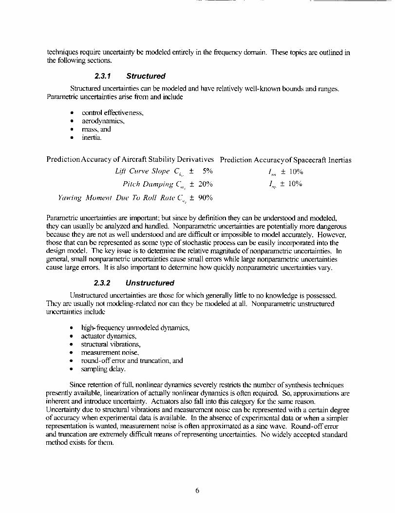
2.3.1 Structured
Structured uncertainties can be modeled and have relatively well-known bounds and ranges.Parametric uncertainties arise from and include
• control effectiveness,
• aerodynamics,• mass, and• inertia.
PredictionAccuracy of Aircraft Stability Derivatives
Li/? Curve Slope CL_' +_ 5%
Pitch Damping C,.... + 20%
Yawing Moment Due To Roll Rate C,,,. + 90%
Prediction Accuracyof Spacecraft Inertias
I,,,, + 10%
/,,z, + 10%
Parametric uncertainties are important; but since by definition they can be understood and modeled,
they can usually be analyzed and handled. Nonparametric uncertainties are potentially more dangerousbecause they are not as well understood and are difficult or impossible to model accurately. However,
those that can be represented as some type of stochastic process can be easily incorporated into thedesign model. The key issue is to determine the relative magnitude of nonparametric uncertainties. In
general, small nonparametric uncertainties cause small errors while large nonparametric uncertainties
cause large errors. It is also important to determine how quickly nonparametric uncertainties vary.
2.3.2 Unstructured
Unstructured uncertainties are those for which generally little to no knowledge is possessed.
They are usually not modeling-related nor can they be modeled at all. Nonparametric unstructureduncertainties include
• high-frequency unmodeled dynamics,
• actuator dynamics,• structural vibrations,• measurement noise,
• round-offerror and truncation, and
• sarnpling delay.
Since retention of full, nonlinear dynamics severely restricts the number of synthesis techniques
presently available, linearization of actually nonlinear dynamics is often required. So, approximations are
inherent and introduce uncertainty. Actuators also fall into this category for the same reason.
Uncertainty due to structural vibrations and measurement noise can be represented with a certain degreeof accuracy when experimental data is available. In the absence of experimental data or when a simpler
representation is wanted, measurement noise is often approximated as a sine wave. Round-off error
and tnmcation are extremely difficult means of representing uncertainties. No widely accepted standardmethod exists for them.
6

2.3.3 Frequency Domain
Classical Control addresses the issue of uncertainty by assuming that all types of uncertainties in
the system cause only gain changes, or phase changes, to occur. Robust Modem Control takes a
frequency domain approach using transfer functions in the S-domain such that certain types of modelingerrors are assumed to have certain frequency effects. Since parametric modeling errors are structureduncertainties with known bounds, they are assumed to cause low-frequency effects. Consequently,
neglected and possibly higher-order dynanaics are assumed to cause high-frequency effects.Unstructured uncertainties, which are not well understood, represent systems in the frequency domain
whose frequencies simply are assumed to lie between some upper and lower bound. Additive
uncertainty is used to model errors in neglected high-frequency dynamics; this represents the absoluteerror in the model. Multiplicative uncertainty, which is used to model errors in actuators or sensor
dynamics, represents the relutive error in a model. This latter type of uncertainty is most useful inrobustness analysis and design.
2.4 Disturbances
Disturbance rejection properties to exogenous disturbances - e.g., gusts, turbulence, wind shear
- are particularly critical in flight control system design. By definition, an exogenous input is one that acontroller cannot manipulate. These unstructured uncertainties are stochastic processes and, as such,
are best represented as stochastic models in terms of mean and variance. The standard gust andturbulence models, due to Von Karman and Dryden, are empirically based and directly applicable to
both controller design and controller analysis.
2.5 Dynamic Inversion Synthesis
DI synthesis is a controller synthesis technique by which existing deficient, or undesirable,
dynamics are canceled out and replaced by desirable dynamics. Cancellation and replacement areachieved through careful algebraic selection of the feedback function. For this reason, this methodology
is also called feedback linearization, it applies to both single-input, single-output (SISO) and MIMOsystems, provided the control effectiveness function (in the SISO case) or the control influence matrix(in the MIMO case) is invertible. The method works for both full-state feedback (input-state feedback
linearization) and output feedback (input-output feedback linearization). A fundamental assumption in
this methodology, is that plant dynamics are perfectly modeled and can be canceled exactly. In practice
this assumption is not realistic, so the new dynamics require some form of robust controller (see Section
2.6.1 ) to suppress undesired behavior due to plant uncertainties. Examples of D1 synthesis are shown in
Chapter 3.
2.6 Robustness
Compensators are designed to satisfy specified requirements for steady-state error, transient
response, stability margins, or closed-loop pole locations. Meeting all objectives is usually difficultbecause of the various tradeoffs that have to be made and because of the limitations of desi_l
techniques. For example, although classical root locus design places a pair of complex conjugate polesto meet transient response specifications, the designer has little control over the location of all other
poles and zeros. The particular property that a control system must have to operate properly in realisticsituations is called robustness. A control system that possesses both good _fisturbance rejection and
low sensitivity is said to be robust. Disturbance rejection is the ability to maintain good regulation(tracking) in the presence of disturbance signals. Low sensitivity is the ability to maintain good

regulation(tracking)in thepresenceof changesinplantparameters.Mathematically,thismeansthatacontrollermustoperatesatisfactorilyfor notjustoneplantbut forafamilyor asetof plants.
Robustnessisdividedinto twodistinctyetrelatedcategories:stabilio, robustness andperjormance robustness. Stability robustness is the ability to guarantee closed-loop stability in spite of
parameter variations and high-frequency unmodeled dynamics. It is important to note that relative
stability, not absolute stability, is of interest in this context. Performance robustness is the ability to
guarantee acceptable performance (settling time, overshoot, etc.) even although the system may besubject to disturbances. The Classical Control method quantifies robustness through gain margin mad
phase margin. Modem Control techniques use the structured singular value analysis of Section 6.2.3 to
quantify robustness. In the MIMO case, both the maximum and the minimum singular values aremeasures of the amplification and attenuation, respectively, of the wansfer function matrices that
represent the family or set of plants of a system. Section 5.1 presents this robustness technique and
demonstrates how to perform the analysis and interpret the results.
2.6.1 �J-Synthesis and H_
Structured singular value synthesis, or _-synthesis, is a multivariable design method that can be
used to directly optimize robust performance. It involves both _-analysis and I-L synthesis.
Performance specifications are weighted transfer functions describing the magnitude and frequency
content of control inputs, exogenous inputs, sensor noise, tracking errors, actuator activity, mad flyingqualities. A family of models (consisting of a nominal model plus structured perturbation models) is used
with magnitude bounds and frequency content specified using weighted transfer functions. All of this is
wrapped into a single standard interconnection structure that is then operated upon by the algorithm.The H_ control controller design methodology is a frequency dormin optimization for robust
control systems. H_ is defined as the space of proper and stable transfer functions - i.e., transfer
functions with a number of zeros less than or equal to the number of poles. The objective is to minimize
the I-L norm. Physically, this corresponds to minimizing the peak value in the Bode magnitude plot ofthe transfer function in the SISO case or the singular value plot in the MIMO case. There are certainadvantages ill minimizing the infinity-norm. These are
• The infinity-norm is the energy gain of the system. By comparison, the Linear Quadratic
Gaussian (LQG) technique minimizes the 2-norm, which is not a gain.
• The infinity-norm minimizes the worst-case root mean square (RMS) value of the regulatedvariables when the disturbances have unknown spectra. The 2-norm minimizes the RMS
values of the regulated variables when the disturbances are unit-intensity, white noise
processes.• H_ control results is guaranteed stability margins (and is therefore robust), whereas LQG
has no guaranteed margins.
As in the Linear Quadratic Regulator (LQR)/LQG methodology, I-L is iterative. In the standard
problem, the solution for the infinity-norm is iterated upon until it is less than a specified scalar value,gamma - known as the gamma iteration. In the optimal problem, the infinity-norm is progressively
reduced until a solution does not exist. In the l-L control problem, the weights are the only design
parameters the user must specify. Constant weights are used for scaling inputs and outputs. Transferfunction weights are used to shape the various measures of performance in the frequency domain;
weights are also used to satisfy the rank conditions. Proper selection of weights depends a great deal
on understanding both the modeling process and the physics of the problem.
Necessary conditions for a solution are the ability to stabilize and detect the system; to performvarious rank requirements on system matrices; and to ensure that the transfer function between
exogenous system inputs and the outputs remains nonzero at high frequencies. This last condition, which
is often violated, occurs because the transfer function is strictly proper; i.e., has more poles than zeros.
8

Solutionsto I-LandLQGproblemsareverysimilar. Bothuseastateestimatorandfeedbacktheestimatedstates,andbothsolvetwoRicattiequationsto computecontrollerandestimatorgains.Thedifferencein thesolutionsliesin thecoefficientsof theRicattiequationandinanextratermin theI-Lsolution.Examplesof thismethodologyarepresentedinChapter5.
2.7 Validation
Validation - which consists of an attempt to match outputs between two different control andsimulation software packages tbr the same control inputs, and for the same controller structure and gains
- was performed on all examples in this document to ensure as much fidelity as reasonably possible.
The degree of fidelity depends on the purpose of the example, the software tool used to synthesize and
simulate the example, the operating system and language, and the platform on which the example wasbeing run.
2.7.1 MATLAB versus MACH
MATLAB and MACH have similar structures that, in theory, should permit good validation.
MATLAB was run on a personal computer (PC) and MACH was run on a UNIX-based workstation.The difficulty involved with this validation effort stemmed from a lack of understanding of the MACH
code itself due to a lack of documentation. Although agreement between the two codes was generally
good, it was inadequate for in-depth investigations and research.
2.7.2 MA TLAB versus Batch Simulation
MATLAB was run on a PC, and the SES batch simulation was run on a Silicon Graphics
Incorporated (SGI) UNIX workstation. Because of adequate documentation and open access to the
SES source code, validation between these two codes proceeded rapidly and with excellent agreement.These two software codes forrn the basis for all of the controller desibm research presented in thisdocument.

3 Applying Dynamic Inversion
3.1 Introduction and Philosophical Approach
This section shows how DI is applied to a relatively simple aircraft control problem. As will be
explained in more detail in Section 4, since the concept of DI itself is quite simple, a controller can be
designed in many different ways. For example, the controller might be either linear or nonlinear. Also, aDI controller is not limited to a first-order inversion. It can take on higher-order forms as well. This
chapter describes one way of designing a Dl-based controller. The steps taken in completing this
design are carefully delineated in the hope that a step-by-step outline will help others design DI-basedcontrollers.
First, a brief outline of the DI process will be given to quickly review the concept, followed by adetailed description of how to design each controller component. Then, aircraft equations of motion are
introduced, and the DI design process is applied to a particular reentry vehicle; i.e., the X-38. Finally,several forms of desired dynamics are presented for this DI application.
3.2 Dynamic Inversion Concept (Linear Aircraft Controller)
As we suggested previously, the basic concept of DI is quite simple. In general, aircraftdynamics are expressed by
,_.=-F(x,u)
y=H(x)(3.1)
where x is the state vector, u is the control vector, and y is the output vector. For conventional uses
(where small perturbations form trim conditions), the function F is linear in u. Equation (3.1) can berewritten as
(3.2)
wherefis a nonlinear state dynamic function and g is a nonlinear control distribution function. If we
assume g(x) is invertible for all values of x, the control law is obtained by subtracting J(x) from bothsides of Equation (3.2) before multiplying both sides by g _(x).
(3.3)
The next step is to command the aircraft to specified states. Instead of specifying the desired
states directly, we will specify the rate of the desired states, _. By swapping J& in the previous
equation to J&_s, we get the final form ofa DI control law.
(3.4)
Figure 3. l shows a block diagram representation of the DI process.
10

Figure 3.1 Dynamic in version process
Although the basic DI process is simple, a few points need to be emphasized. First, althoughwe assume g(x) is hwertible lbr all values of x, this assmnption is not always true. For example, g(x) is
not generally invertible if there are more states than controls. Furthermore, even ifg(x) is invertible (i.e.,
g(x) is small), the control inputs, u, become large; and this growth is a concern because of actuatorsaturation. Since the dynamics of the actuators, as well as sensor noise in the feedback loop, are
neglected during this primitive controller development to illustrate the process, a "perfect" inversion is
not possible.
DI is also essentially a special case of model-following. While it is similar to other model-following controllers, a DI controller requires exact knowledge of model dynamics to achieve good
performance. Robustness issues therefore play a significant role during the design process. (This issue
is discussed in detail in Chapter 5.) To overcome these difficulties, a DI controller is normally used asan inner-loop controller in combination with an outer-loop controller designed using other control design
techniques.
The closed-loop transtbr function for a desired CV that is being inverted is found according to
Figure 3.2. From this block diagram, we can observe that the desired dynamics operate on the error
between the commanded CV and its feedback term. In this figure, the pure integrator on the right sideis used to approximate the rest of the system dynamics, as shown on the right side of the blockdiagram _2. The CV here corresponds to the state x in the previous development as well as in Figure3.1.
r m
cvcm lovesDesired I _..! -- L._II_
Dynamics : S]'_-] I
" -- Actuators
Dynamic InversionEffector Allocation
Airplane DynamicsSensors
Figure 3. 2 Block diagram to calculate closed-loop tran,_[er.[unction
3.2.1 Simplified Longitudinal Controller for an Aircraft
A simplified foml of the linear longitudinal equation for an aircraft's pitch axis considers only the
pitching moment equation.
M,_a+ Mqq+ Mae6e (3.5)
11
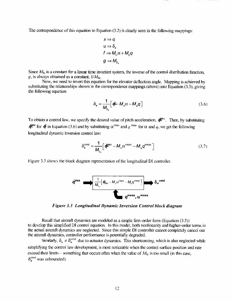
The correspondence of this equation to Equation (3.2) is clearly seen in the following mappings:
x_q
u_8 e
f _M,_oc+Mqq
g_M_.
Since M_ is a constant for a linear time invariant system, the inverse of the control distribution function,g, is always obtained as a constant, 1/M_.
Now, we need to invert this equation for the elevator deflection angle. Mapping is achieved bysubstituting the relationships shown in the correspondence mappings (above) into Equation (3.3), giving
the following equation:
1(3.6)
To obtain a control law, we specify the desired value of pitch acceleration, _s. Then, by substituting
_s for _ in Equation (3.6) and by substituting ocn'_'_'and q m_,_for oc and q, we get the following
lonlctudinal dynamic inversion control law:
5c..,o, 1 [,_so -Moo (3.7)
Figure 3.3 shows the block diagram representation of the longitudinal DI controller.
(_des
:_lm qmeas, _meas
Figure 3.3 Longitudinal Dynamic Inversion Control block diagram
Recall that aircraft dynamics are modeled as a simple first-order form (Equation (3.5))
to develop this simplified DI control equation. In this model, both nonlinearity and higher-order terms in
the actual aircraft dynamics are neglected. Since this simple Dl controller cannot completely cancel outthe aircraft dynamics, controller performance is potentially degraded.
Similarly, 6_ ¢: 6_r_o due to actuator dynamics. This shortcoming, which is also neglected while
simplifying the control law development, is most noticeable when the control surface position and rate
exceed their limits - something that occurs often when the value of Ma, is too small (in this case,_cmd was unbounded).
12

Finally,o_me°s:xcz; qrOeos :X:q due to sensor processing. This factor is also neglected in the
control law development, thereby potentially harming controller performance as well.
3.2.2 Simplified Lateral Directional Controller for an Aircraft
Lateral/directional DI control equations are developed in this section. Although the
development procedure is similar to that of the longitudinal case, we need to simultaneously deal withtwo states (roll rate and yaw rate) controlled by two control surfaces (ailerons and rudders) instead of
with one state (pitch rate) controlled by one control surface (elevator) as in the simplified longitudinal
case.Simplified linear lateral aircraft equations can be written with respect to roll as well as yaw axes
as
Lpp + Lrr + !.._ + Lsfsa 4- L_6r
_=- Npp+ Nrr + N#[3 +N_o&a + N_6r(3.8)
lfwe write Equation (3.8) in a compact matrix form, we get
ILLr IIi]+EL (3.9)
When we compare the matrix form of Equation (3.9) to Equation (3.2), each parameter is either avector or a matrix but the form remains the ,same.
u = -6o]__r
f= L_
N_
L_,g=
N_
L_ Lp ]
N r N_ J
L_,
(3.10)
Notice here that the control distribution matrix, g, is a square matrix. Therefore, its inverse exists in
general.As a next step similar to the longitudinal case, we will invert the roll rate and yaw rate dynamic
equations to obtain aileron and redder deflection angles.
13
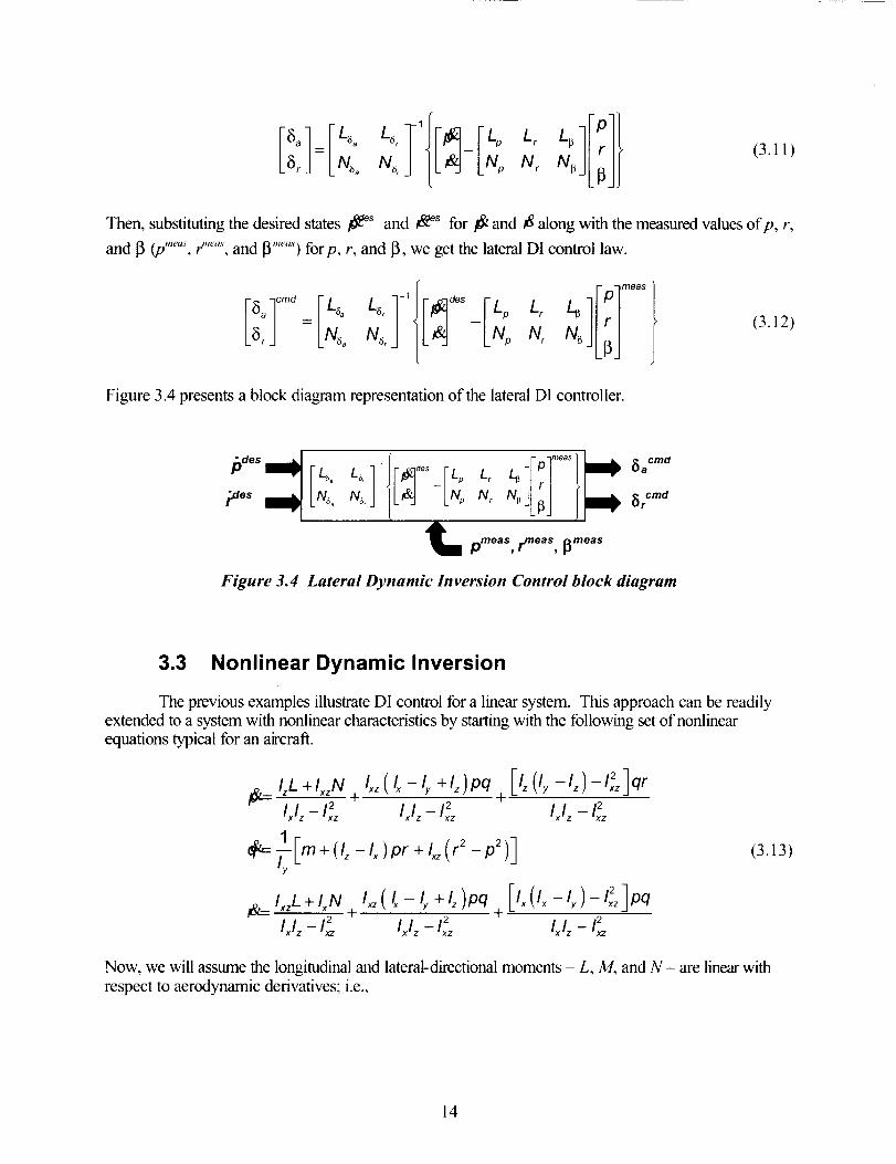
rLaLrll{ Lr (3.11)
Then, substituting the desired states /_es and _s for ,_ and ,_ along with the measured values of p, r,
and [3 (p,,e% F,,,_,,, and [3"'_"_)for p, r, and 13, we get the lateral DI control law.
I-p-I'e_s
ll;lN_(3.12)
Figure 3.4 presents a block diagram representation of the lateral DI controller.
'_ p,,,eas, rmeas,_r,,eas
Figure 3.4 Lateral Dynamic Inversion Control block diagram
3.3 Nonlinear Dynamic Inversion
The previous examples illustrate DI control for a linear system. This approach can be readilyextended to a system with nonlinear characteristics by starting with the following set of nonlinear
equations typical for an aircraft.
I_= IzL +l_zN + I_z( Ix - ly +lz)pq 4 [Iz (ly -Iz)-Ix_ ]qr
Uz- I_xz Uz- I_z Uz- I:_
_Y.=_[m+(Iz-lx)Pr +l_(r2-p2)l
__lJ_+lxN_Ix_(l_-I_+lz)Oq+[Ix(Ix-I_l-I_lpqUz- I_ Uz- I_z txIz- t_
(3.13)
Now, we will assume the longitudinal and lateral-directional moments - L, M, and N - are linear with
respect to aerodynamic derivatives; i.e.,
14

L = _[3+ L,_5 a +L,_ 5,. +Lpp +Lrr
M = Mot + Mqq + Mae_)e
N = N_# + Na. 5_ + N_r 5: + Npp + Nrr
By substituting the above linear moment equations into Equation (3.13), we can obtain a relation in
Equation (3.15) that combines linear and nonlinear terms.
Otl
[i 0Lr] I0LLl[ e1= 00MqOPI+M_O 0 8_
N_ N o 0 N_ q l 0 N_, N< _)r
rl
+ [ o 1[l_(r2-p2)+(Iz-lx)pr[
L-Ixz o I, j -Ix_qr { ( l_ I If ) pq J
If the last term is ignored, the result is identical to the linear set of DI equations previously obtained.
Finally, inverting the above equation as well as performing proper substitutions of the commanded,
desired, and measured values gives the resulting DI control law.
libelI_el cmd [_ C6a C6']-ll[_des I! Lo0 Lp O Lr p
6_ = o 0 0 - ,_ 0 Mq 0 p
5_ N_o N< Np Np 0 N r
-1 I meas meas .{_(ly_lz)qmeasrmeas
[10 0--_xz] [ (IrXZm_as2qPmeas2 pmeasrmeas
- ¢_ /,_ - )+(&-L)
L-/xz o I_ j _lx_qm_rmO_s +(Ix_ly)pm_a_qmO_
(3.14)
(3.15)
(3.16)
3.4 Applying the Dynamic Inversion Controller tothe X-38 - the Overall Structure
The DI control laws developed in the previous sections are now integrated into an overall
control structure. As the block diagram ill Figure 3.5 shows, DI control is used as an inner loop
accompanied by o_ and • feedback outer loops. Although any type of control technique can be used
for the outer loop, simple feedback is used in this particular example to illustrate the characteristics of
inner-loop DI control.
15

(X cmd (_ error
p cmd i_ des
qcmdCommand _ DesiredInverter Dynamics
k
p_5 pt/_OS
qm_ q._r_S rm_
Se n sor
DynamicInversion
i_acmd
cmd
ControlSurface
l X-38 l OuModel
Figure 3.5 Overall Dynamic Inversion Control block diagram
Lput
The overall D1 controller requires commanded values of angle-of-attack, otc''_, and bank angle,
0 ''''a, as inputs. Then, the measured values of o_''''_' and 0 '''°"_'are subtracted from the con_aanded
values to produce (_e,-,.o,-and 0'""" in the outer loop. These error values are then fed into the Command
Inverter block to be changed to rate commands, p"'"/, ""/ r '''''_q , and . The Desired Dynamics block uses
these rate commands and the rate measurements to create the desired acceleration terms - favored
forms of commands for the DI controller. The next block is the DI block, which produces the control
surface deflection angle corrrnands (3,,_'''/, _5,5''d, and 5,.'""'( Finally, the control surface commands are
fed into the Plant block, X-38 Model, via the Control Surface block. The Control Surface block
includes control surface management logic, which blends the three command values, 8,, c'''/, 5,5 '''/, and
_,.'"'_, into two command values, _LL''''_ and _),5'''/, that include the dynamics of the actuators as well as
the position and rate limits of the actuators. Gust and sensor noises are added to the system as external
disturbances as well.
3.4.1 Command Inverter
In aircraft applications, sometimes it is better to command displacements in the angle-of-attack
and bank angle rather than command the body axis rates p, q, and r. However, rate commands are
needed as inputs to the Desired Dynamics block. The Command Inverter block (Figure 3.6) changesdisplacement commands into rate commands so that displacement cormaands are directly implemented
in the DI controller. This section describes how displacement commands are transformed into ratecommands.
16
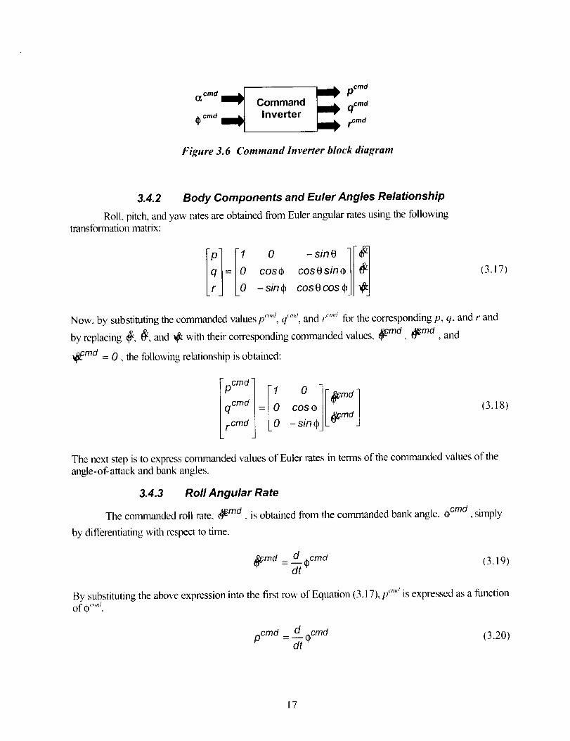
Command qcmd
(_ cmd Inverter r cmd
Figure 3. 6 Command Inverter block diagram
3.4.2 Body Components and Euler Angles Relationship
Roll, pitch, and yaw rates are obtained from Euler angular rates using the followingtransformation matrix:
I!1i!° s,nolIO= cos_coso_n_//_I-sin, cosocos,JLej
(3.17)
Now, by substituting the commanded values pC,,,,_, ,.,,,J rc,,,,/q , and for the corresponding p, q, and r and
by replacing _, _, and _ with their corresponding commanded values, _md (_md and
_md = O, the following relationship is obtained:
F1 l, 0 ll,m,1qCmO/:0 cosOjL_m_jr cmd | 0 - sin ¢J
(3.18)
The next step is to express commanded values of Euler rates in terms of the commanded values of the
angle-of-attack and bank angles.
3.4.3 Roll Angular Rate
The commanded roll rate, _ma, is obtained from the commanded bank angle, 0 cmd , simply
by differentiating with respect: to time.
_md d ocmd (3.19)=--__
By substituting the above expression into the first row of Equation (3.17), 1/'''l is expressed as a function
of O''''J.
pcmd d ocmd=-_-_ (3.20)
17

3.4.4 Pitch Angular Rate
Expressing pitch angular rate, _ma, from angle-of-attack is slightly more complicated than the
roll angular rate case. First, the Euler pitch angle can be expressed in terms of o_ (angle-of-attack), [3
(sideslip angle), 3I (flight path angle), and _ (bank angle) by
where:
0 = tan -1 ab+ Jndf_- e b ]a 2 _ sin 2 y J
a = cosc_ cos
b = sin$sin_ + cos #sino_cos
The commanded value of the Euler pitch rate is calculated by differentiating the commanded value of
Euler pitch angle by
(3.21 )
do. (3.22)dt
Substituting this expression for _ into the second row of Equation (3.17), q,,,.i is expressed as a
function of 0 '''l.
(3.23)1
with Ocmd = tan-1_ sin 2 y+aCmdb cmd +sin74(acmd)2 (bCmd) 2
aCm d )2 _ sin2 Y
where:a cmd = COS o_cmd COS
b cmd -= sin(p cmd sin_ + cosO cmd sino_ cmd cos
3.4.5 Yaw Angular Rate('md
Instead of defining the corresponding Euler pitch and yaw rate commands to r , we simply setr ''''¢ equal to zero.
r cmd = 0 (3.24)
18

3.5 Multiple Time Scale Method
To bypass a singularity problem in the inversion of an ineffective control matrix, a multiple time
scale method has been developed that has been found to be quite successful in solving the problem.This approach is especially useful when inverting slow-motion variables, such as angle-of-attack, o_, in
the longitudinal case and sideslip, !3, and bank angle, 0, in the lateral/directional case. These variablesare deemed as "slow" dynamics because the control effectiveness on their dynamics is quite low.
Variables making up the "fast" aircraft dynamics include pitch rate, q, in the longitudhml case, roll rate,
p, and yaw rate, r, in the lateral/directional case. Since the control effectiveness on these body rates is
high, these dynamics are considered "fast" dynamics. The multiple time scale method thus seeks toreformulate the original differential equation (Equation (3.1)) into a set of two separate differential
equations consisting of a set of slow dynamics, _, and a set of fast dynamics, ,8,.
ff_- f( x)+ g(x)y (3.25)
_= h(x,y )+ k(x,y)u (3.26)
Applying this technique to the linear aircraft dynamics, £a= Ax + Bu, yields the following slow dyl_-nic
equations for the rate variables (Equation (3.27)) and fast dynamic equations for the acceleration
variables (Equation (3.28)):
(3.27)
51
[o....oo °+'LO ° ]o.... ql
r I
(3.28)
where A and B represent the longitudinal state and control input matrix values for the linear state-spacemodel, and A and B repre_nt the lateral/directional state and control input matrix values. Also, the
subscripts denote the row and column value, respectively. Note that in Equation (3.27), rate variables
form the input for the slow dynamics while the actual control surface commands form inputs for the rate
dynamics shown in Equation (3.28). Inverting each set of differential equations generates two D1control laws, one for the outer DI loop lEquation (3.29)) and one for the inner DI loop (Equation(3.30)).
Iil 0lt(i]lA 00j/i](3.29)
19

II -- 2 0 0 0 A:_ 3
A block diagram representation of this 2-time scale approach is shown in Figure 3.7.
O_
P
q
r
(3.30)
_cmd Pcmd _a,cmd
l_cmd qcmd _e,cmd
0 l anan _ Slow Fast ActuatorInversion Inversion Dynamics _
TI t !p
qr
Figure 3. 7 Block diagram of the 2-time scale approach
C¢
In the Fast Inversion block, fast desired dynamics are calculated and the control law in Equation
(3.30) is implemented. Fast dynamics are a function of the CV commands, (p_,,,_, qc,,d, and rc,,,t) and
their feedback terms (p, q, and r). Similarly, in the Slow Inversion block slow desired dynamics arecalculated and the control law (Equation (3.29)) is implemented. Again, slow dynamics are a function
of the CV commands (_c,,,,/, 13c,,,/, and 0c,,,_) and their feedback terms (o_, 13, and 0). In summary, the
Slow Inversion block produces the commanded rate variables of Equation (3.29) that are fed to thedesired dynamics in the Fast Inversion block. Using these fast desired dynamics, the fast inversion
control law of Equation (3.30) produces the commanded control deflections that are sent to the controlsurface actuators, which then serve as input to the inherent dynamics.
Several observations can be made from these two DI control laws. First, only the short-periodaerodynamic terms (A22, A23, A32, and A33) are present in this set of slow and fast dynamics. Further,these two equations combine, retaining all original lateral/directional state matrix terms. It is also
irr_rtant to observe that the control effectiveness of the elevon on angle-of-attack, B2_, is not presentin the inversion matrix and has actually been eliminated altogether from these two sets of equations. This
is the term that traditionally causes a singularity effect on inversion because the value is typically small inmagnitude. Instead, the control effectiveness on the pitch rate dynamics, B2__,has been retained for
inversion in the fast DI control law. Similarly, control input matrix values affecting sideslip and bank
angle dynamics have also been eliminated (B_ n, Bj2, B41, and B42). Therefore, only the control matrixterms for the rate dynamics have been kept (B2_, B22, B3_, and B32). This is of benefit because the
control surfaces are more effective on the rotational rate variables than they are on the rotational
variables. Finally, it is important to emphasize the fact that this 2-time scale method requires that thedesigner specify two sets of desired dynamics: one set for the slow dynamics and one set for the fast
dynamics.
20

3.6 Desired Dynamics
The Desired Dynamics block, which was introduced during DI control law development, is
explained in detail in this section.DI control requires acceleration terms. For example, as the following longitudinal DI equation
shows, a desired value of pitch angular acceleration, _, is required:
M5 e
(3.25)
However, applications normally use either displacements or rates as command states to control the
system. The Desired Dynamics block acts as a mapping function between the rate commands and thedesired acceleration terms, which are the required foma for the DI equations. The structure of the
Desired Dynamics block is shown in the flow chart in Figure 3.8.
I Given 1Is by Idynamic inversion
Choose feedback 14
_Lyes [
_'_om plete_ _
Provide anti-windup IprotectionI
yes
+Parameterize Igain selection
I
Figure 3. 8 Desired dynamics development Jot dynamic inversion
(adapted from Ref. 12)
Several forms of desired dynamics are presented in this document and are evaluated in terms of
performance and robustness. The different forms of desired dynamics consist of
21

• Proportional dynamics _3
• PI dynamics 12* Flying quality dynamics 14
• Ride quality dynamics
3.6.1 Proportional Case
The simplest way of achieving desired dynamics implementation is the proportional, or first-
order, case. In this case, the desired dynamics are expressed as
CVa_ = K,o(CVcm d -CV). (3.31)
The K_ term in Equation (3.31) sets the bandwidth of the response. The bandwidth must be selected
to satisfy time-scale separation assumptions without exciting structural modes or becoming subject tothe rate limiting of the control actuators. Figure 3.9 shows the block diagram representation of the
Proportional Desired Dynamics block introduced in this section.
Xcmd
Figure 3. 9 Proportional Desired Dynamics block diagram
As shown above, the constant K,0 amplifies the error between the CV command and its feedback term.
In Figure 3.9, CV is represented as the state, x. So, the closed-loop transfer function for the
proportional form of desired dynamics, shown in Equation (3.32), desires to place a single pole at
s = -K_o.
CV _ K_o
C Vc,,,d s + K,,,(3.32)
3.6.2 Proportional Integral Case
The Desired Dynamics block is not limited to a first-order component. If the Desired Dynamicsblock does not create satisfactory handling qualities (for piloted aircraft) using a set of first-order
equations, a higher-order system is used. A commonly used higher-order block is a PI. This form is
particularly popular in DI literature that uses fighter aircraft examples _-''15. This type of Desired
Dynamics block structure is also used in the linearized MACH controller designed by Honeywell for theX-38 vehicle and has been adopted for this study as well. The block diagram representation ofa PI
desired dynamics component is shown in Figure 3.10. It has the same form as that used in theHoneywell study _2with a KR of 5 sec _ selected.
22
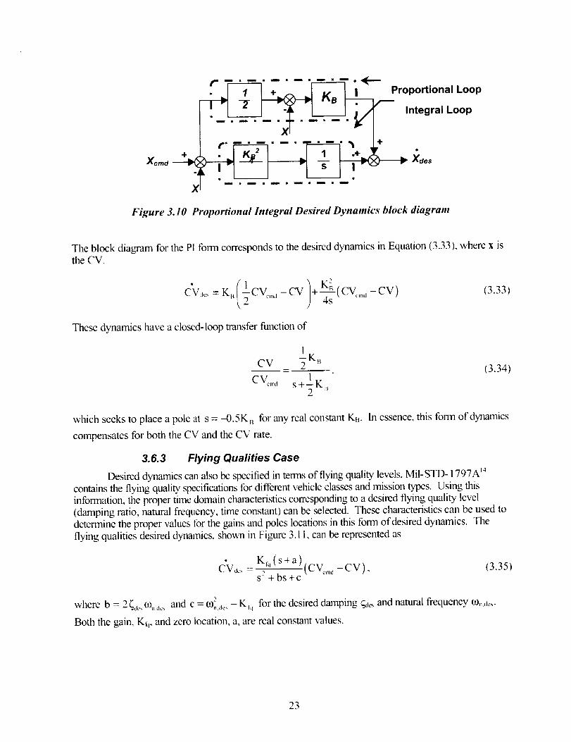
Xc,.
X
r --r--z--m-n..... _-- •
4 KB " Proportional Loop
i. _ .-_ _ ;//-- Integral Loop
...... X_ .... _:
. t KJ r t 1 t .+ _r •
_-_"_'_l _S-_ -_)-_l_Xdes.m _4m • m • m • m • m
Figure 3.10 Proportional Integral Desired Dynamics block diagram
The block diagram for the PI fbrm corresponds to the desired dynamics in Equation (3.33), where x isthe CV.
-K.( 1 /+ N_ (CV_,.. -CV)CV_,_ -2 CV_'ma-CV ) 4s(3.33)
These dynamics have a closed-loop transfer function of
! KCV _ B
_- - (3.34)1
C V_,.L_ s+-K_2
which seeks to place a pole at s = -0.5Kf_ for any real constant K_. in essence, this form of dynamics
compensates for both the CV and the CV rate.
3.6.3 Flying Quafities Case
Desired dynamics can also be specified in terms of flying quality levels. MiI-STD- 1797A _4
contains the flying qualitty specifications tbr different vehicle classes and mission types. Using thisinformation, the proper time domain characteristics corresponding to a desired flying quality level
(damping ratio, natural frequency, time constant) can be selected. These character/sties can be used todetermine the proper values lbr the gains and poles locations in this form of desired dynamics. The
flying qualities desired dynamics, shown in Figure 3.11, can be represented as
C'Vd_._- K,.q (s+a)_ (CV.,,,d-CV) , (3.35)s +bs+c
0.) 2where b = 2 _,_ c0,,.a_ and c = , id__ --Kt, _ for the desired damping _l_, and natural frequency m_,d_.
Both the gain, K_, and zero location, a, are real constant values.
23

+
Xcmd
1
K).q(S +a) _ _es
s2 +bs+c |
Figure 3.11 Flying Qualities Desired Dynamics block diagram
The closed-loop transfer function for the flying qualities dynamics is given in Equation (3.35).
These dynamics desire to place three closed-loop poles and to add a single zero to the system.
CV _ K,_) (s +a)
C g, md s 3+ bs-' + (c + K,_,)s + K,.,,a(3.36)
3.6.4 Ride Qualities Case
The ride qualities form of desired dynamics that can also be used in DI are given in Equation(3.37) and represented pictorially in Figure 3.12.
K., (CV_,,d _CV )s+b
(3.37)
,tk
Xcmd
Figure 3.12 Ride Qualities Desired Dynamics block diagram
The closed-loop transfer function for this set of desired dynamics is given below by
CV __ Krq
CVcm d s 2• +bs+ K,q(3.38)
which desires two places to closed-loop poles at s_,2 = -0.5b _0.5_/b- - for real constants b4K,qi
and K,.q.
For highly augmented airplanes, the control arficipation parameter (CAP) re4Placesthelongitudinal short period requirements, such as damping ratio and natural frequency _ . The desired
longitudinal dynamics are instead designed by selecting a desired damping ratio and CAP value.Equation (3.39) shows how to calculate CAP for a specific load factor rb and natural frequency.
co_CAP = --
n(z
(3.39)
24

The flying quality levels for various CAP and _sp values are shown in Figure 3.13.
Inherent
Dynamics
_ IIIIIIII.
I _] Level 31 (_2 [..._.._
101 10 0
Short Period Damping Ratio, _ sp
¢¢
¢1
ll
ld
Figure 3.13 Control anticipation parameter requirements Jbr highly augmented vehicle
Once a CAP and a (.sp are selected to satisfy a desired flying quality level, tile desired short-
period natural frequency can be calculated from Equation (3.39). The gain and the pole location for theopen-loop desired dynamics are then backed out from these two specifications, _sp and c%.sp. For
example, the desired dynamics (see Figure 3.13) correspond to the following:
• CAP=0.802
• _sp =0.8
Using the CAP equation yields a desired c0,,.sp of 1.4s _. The corresponding gain and pole locations are
then found according to Equations (3.40) and (3.41), respectively.
K_q = m_.sp = 1.96 (3.40)
-b : -2_s,, K_, q : -2 _pO),, s,, : -2.24 (3.41)
The desired dynamics for this example become
g
CVdes -
1.96
s + 2.24(CVc,,_ , -CV). (3.42)
25
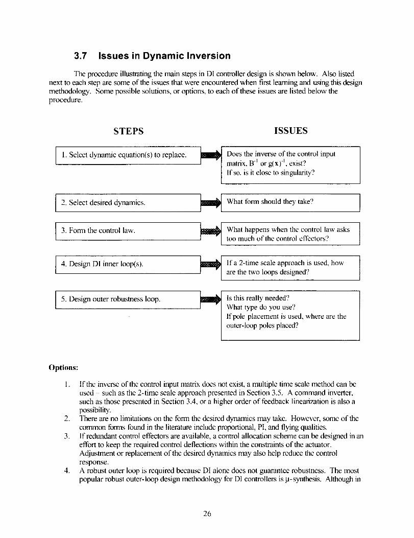
3.7 Issues in Dynamic Inversion
The procedure illustrating the main steps in DI controller design is shown below. Also listed
next to each step are some of the issues that were encountered when fast learning and using this designmethodology. Some possible solutions, or options, to each of these issues are listed below the
procedure.
STEPS ISSUES
1. Select dynamic equation(s) to replace.
2. Select desired dynamics.
3. Fon-n the control law.
Does the inverse of the control input
matrix. B-t or g(x) t, exist?
If so, is it close to singularity?
4. Design DI inner loop(s).
5. Design outer robustness loop.
What form should they take?
What happens when the control law askstoo much of the control effectors?
If a 2-time scale approach is used, how
are the two loops designed?
Is this really needed?
What type do you use?
If pole placement is used, where are the
outer-loop poles placed?
Options:
1. If the inverse of the control input matrix does not exist, a multiple time scale method can beused - such as the 2-time scale approach presented in Section 3.5. A cornmand inverter,
such as those presented in Section 3.4, or a higher order of feedback linearization is also apossibility.
2. There are no limitations on the form the desired dynamics may take. However, some of the
common forms found in the literature include proportional, PI, and flying qualities.
3. If redundant control effectors are available, a control allocation scheme can be designed in an
effort to keep the required control deflections within the constraints of the actuator.Adjustment or replacement of the desired dynamics may also help reduce the control
response.4. A robust outer loop is required because Dl alone does not guarantee robustness. The most
popular robust outer-loop design methodology for DI controllers is B-synthesis. Although in
26

the literature LQG is not as well published in regard to DI controllers, LQG has been shownto be effective, as shown in Section 5.2. LQR is another possibility for robust outer-loop
design as well.
27

4 Simulation
In this chapter, the simulation component buildup is presented for the X-38 reentry vehicle, andthe DI design process is then applied to the vehicle model. Simulation results are shown and discussed
for three D| design examples to give the reader more detail on how the design process is carried out.
4.1 Control Surfaces
The Control Surfaces block (Figure 4.1) is composed of two sub-blocks, the Control Surface
Management Logic sub-block and the Actuator Dynamics sub-block. A conventional aircraft is usuallyequipped with three control surfaces; namely, a rudder, an elevator, and an aileron. But, the X-38 has
only two sets of control surfaces - rudders and elevons. Control Surface Management Logic must
therefore blend three inputs into two inputs so that commands can be fed smoothly into the ActuatorDynamics sub- block.
(_r cmd
(_e cmd
_)aCmd
Control Surface
RcmdControlSurface Actuator
Management Dynamics
Logic
Figure 4.1 Control Surfaces block diagram
4.1.1 Definitions (from the X-38 Aerodynamic Design Data Book)
The X-38 vehicle has two sets of control surfaces (see Figure 4.2): a pair of elevon control
surfaces, located on the lower rear of the vehicle; and a pair of rudders, one at the top of each of thevertical fins. The positive direction of deflection for the elevon is down (as shown in Figure 4.2), and,
looking from the rear, to the left for the rudders. Both elevons and rudders are dual-function control
surfaces. Each surface is deflected independently to provide the required control authorities.
28
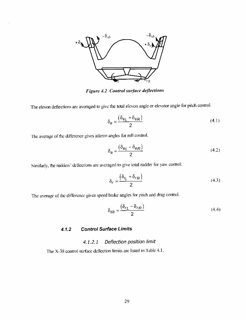
. ,_m7. _ T ,JeR
Figure 4.2 Control surface deflections
The devon deflections are averaged to give the total elevon angle or elevator angle for pitch control.
_e = (_el + _eR)2
(4.1)
The average of the difference gives aileron angles for roll control.
(_eL -_)eR)
2(4.2)
Similarly, the rudders' deflections are averaged to give total redder for yaw control.
_r-
)rL + _rR )
2(4.3)
The average of the difference gives speed brake angles for pitch and drag control.
_sb =(SrL - _)rR )
2(4.4)
4.1.2 Control Surface Limits
4.1.2.1 Deflection position limit
The X-38 control surtace deflection limits are listed in Table 4.1.
29
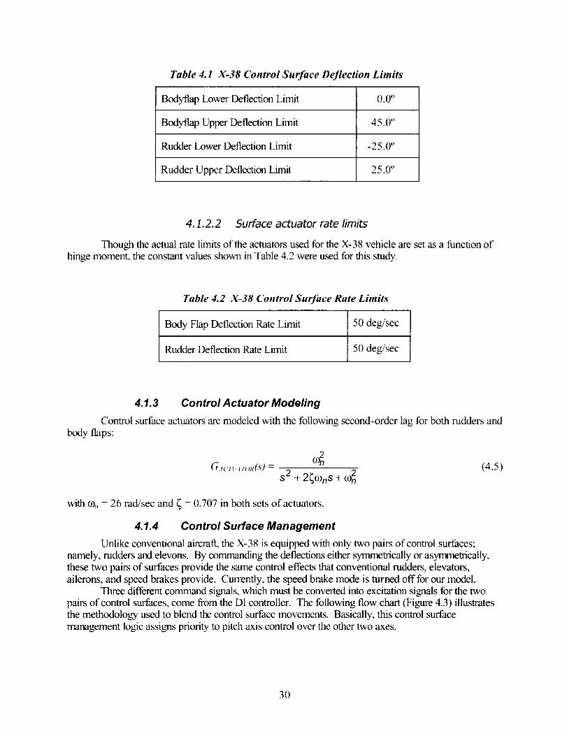
Table 4.1 X-38 Control Surface Deflection Limits
Bodyflap Lower Deflection Limit 0.0 °
Bodyflap Upper Deflection Limit 45.0 °
Rudder Lower Deflection Limit -25.0 °
Rudder Upper Deflection Limit 25.0"
4.1.2.2 Surface actuator rate limits
Though the actual rate limits of the actuators used for the X-38 vehicle are set as a function of
hinge moment, the constant values shown in Table 4.2 were used for this study.
Table 4.2 X-38 Control Surjbce Rate Limits
Body Flap Deflection Rate Limit 50 deg/sec
Rudder Deflection Rate Limit 50 deg/sec
4.1.3 Control Actuator Modeling
Control surface actuators are modeled with the following second-order lag for both rudders and
body flaps:
G,4CT_'..j r(m(S) = 0)2
S 2 + 2((0nS + (02(4.5)
with (0, = 26 rad/sec and _ = 0.707 in both sets of actuators.
4.1.4 Control Surface Management
Unlike conventional aircraft, the X-38 is equipped with only two pairs of control surfaces;
namely, rudders and elevons. By commanding the deflections either symmetrically or asyrlrnetricaily,these two pairs of surfaces provide the same control effects that conventional rudders, elevators,
ailerons, and speed brakes provide. Currently, the speed brake mode is turned off for our model.
Three different command signals, which must be converted into excitation signals for the two
pairs of control surfaces, come from the D! controller. The following flow chart (Figure 4.3) illustrates
the methodology used to blend the control surface movements. Basically, this control surfacemanagement logic assigns priority to pitch axis control over the other two axes.
3O

START
7
]Figure 4.3 Eievon control management iogic flow chart
Since optimization of the control surface allocation is beyond the scope of this study, a very
simple surface management logic is developed and employed here. However, this allocation is animportant aspect of the ultimate design of the flight control system. An important question yet to beanswered is whether the DI design process flows naturally into this optimization scheme, or whether it
makes optimization more obscure. Figures 4.3 (above) and 4.4 (below) illustrate control surface
management logic for rudders and elevons.
START
:rod
7
Figure 4.4 Rudder control management logic flow chart
31

4.2 Sensor Modeling
As in other aircraft, direct measurement of sideslip angle on the X-38 is highly uncertain. So,
the sideslip angle is estimated by combining other measurements. The following equation is one way toestimate sideslip angle. An integral form of this equation is used in simulations for this study.
_#st _ Yp p +
v_neas
Yrv_'neas _,lrrneaS+lv:easlOrne s+l"rt,rn easv_neas
(4.6)
All other parameters are assumed to be measurable. White noise is added to the outputs to mimicsensor noise.
4.3 Gust Modeling
Gust effects, modeled as a disturbance, are also considered when evaluating the DI controller.
Gusts are added to the body component velocity of the vehicle as shown in the following block diagram
(Figure 4.5). Typical gust inputs are also shown in Figure 4.6.
Gust Model Input
Body ComponentVelocities
Output Velocities
Figure 4.5 Gust modeling
lTime
_L
t_
lib
Time r
Figure 4. 6 Typical gust inputs
32

4.4 Comparison Between MACH Controller and TAMU
Design
4.4.1 Control Variable Definition
Derivatives of the state variables p, q, and r are used as CVs for the X-38 DI exarnple. Instead
of specifying p, q, or r, however, MACH specifies the dynamics of the derivative of the CVs. The CV
vector has three components: L C V, MCV, and NC V. Each of these components controls roll, pitch,
and yaw moments, respectively. The variables are defined as follows:
_ LCV-]
CV=|MCVILNCVj
(4.7)
with
LCV = Ps (4.8)
, , nz+ --cosycosja - Ps tan_ +K#_- coSY_v l (4.9)MCV =q4 Vco (S+Xnz) Vcos[_ Vco
NCV = rs + K#_ - g cos ysinp(4.10)
In these equations, g represents the bank angle about the velocity vector.
Since the CVs are no longer states themselves but are combinations of states, a CV definitionblock was added to our Simulink example to "upgrade" to the MACH-generated controller. Although
differences in roll axis CVs are minor, they can occur in either body-axis roll rates with flight path
components or in stability axes. And although the definitions ill pitch and yaw axes CVs for the MACHconlroller differ from this example, both have a strong angular rate content. Because the first terms on
the right side of each equation dominate, MCV and NCV essentially become q and r, respectively, in
our example controller.
4.4.2 Desired Dynamics Module
The Desired D3alamics module of the MACH controller is, in form, a PI controller thatis identical to our Sinulink example in Figure 3.10. It has the same magnitude of bmflwidth, Ku, of 5sec _ as well.
4.4.3 Dynamic Inversion
The MACH controller starts with the same nonlinear fon-n for the vehicle equations of motion as
outlined in Section 3.2.
_&= F(u,x ) (4.11)=f(x)+g(x)u
33

where x
CVs in MACH are functions of the state variables,
CV =CV(x),
where CV is the CV vector defined in Equation (4.7). Then,
acv acvcv- _-_
_x _x
So, the DI control law can be obtained as
is the vector of state variables and u is the vector of control effectors. Recalling that the
(4.12)
_CV , ,
f(x)+'-_-x gtx)u. (4.13)
u = g(x) CV ax
4.4.4 Control Effector Priority (Surface Management)
As was previously explained in Section 3.2, the first bracket in the right side of the DI control
law must be a square matrix so it can be inverted. This mathematical requirement means that the
number of control effectors must equal the number of CVs. In the MACH application, the row
dimension of aCV is 3; therefore, the column dimension of g(x) must be 3 as well to have a squarebx
matrix. Thus, three control effectors are required. Since the three CVs in MACH have a strong angular
rate content and the X-38 has three moment-producing controls (differential elevons, symmetric
elevons, and rudders), the vehicle has an appropriate number of control effectors for three of the four
flight control modes listed in Table 4.3.
Mode FlightMode
1 ACS Only
Blended2
ACS
3
4
Table 4.3
Flaps
Only
Rudders
and Flaps
MA CH 1/201 Flight Control Modes
# ofConditions CV Feedback
CVs
qb,,, < 2 3 INS: p, q, t-,
2 < qhar < 33O
ql,,,,. > 302
and M < 6
M >6 3
INS: p, q, r, _, N:
NAVDAD: or, V, qb,,,.
INS: p, q, r, N_-
NAVDAD: o_,I_\ q_,,,,.
INS: p, q, r, N_, N,
NAVDAD (or FADS):
tz, V, %,1,
# of
Effectors
3
5
2
3
Effectors
Tx, T,,T:
L,T,,L, 8,,,8,,
8,,,8,.
8,,, &, 8,.
34
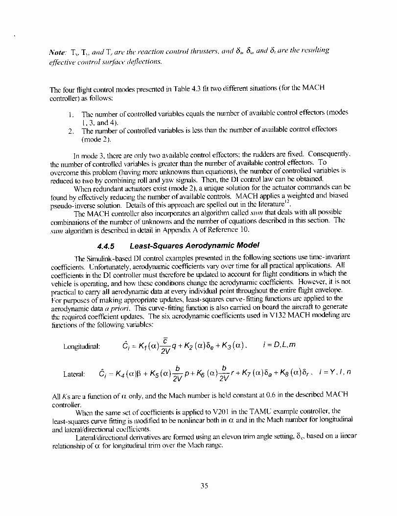
Note." T_, T:, attd T, are the' reaction control thrusters, and fi._ _, and fir are the resulting
elYective control sur_tce dejlections.
The four flight control modes presented in Table 4.3 fit two different situations (for the MACHcontroller) as follows:
1. The number of controlled variables equals the number of available control effectors (modes1,3, and 4).
2. The number of controlled variables is less than the number of available control effectors
(mode 2).
In mode 3, there are only two available control effectors; the rudders are fixed. Consequently,the number of controlled variables is greater than the number of available control effectors. To
overcome this problem (having more unknowns than equations), the number of controlled variables is
reduced to two by combining roll and yaw signals. Then, the DI control law can be obtained.When redundant actuators exist (mode 2), a unique solution for the actuator co_runands can be
found by effectively reducing the number of available controls. MACH applies a weighted and biasedpseudo-inverse solution. Details of this approach are spelled out in the literature _-'.
The MACH controller also incorporates an algorithm called sum that deals with all possible
combinations of the number of unknowns and the number of equations described in this section. The
sum algorithm is described in detail in Appendix A of Reference 10.
4.4.5 Least-Squares Aerodynamic Model
The Simulink-ba,sed D I control examples presented in the following sections use time-invariant
coefficients. Unfortunately, aerodynamic coefficients vary over time for all practical applicat/ons. All
coefficients in the DI controller must therefore be updated to account for flight conditions in which the
vehicle is operating, and ho,a these conditions change the aerodynamic coefficients. However, it is notpractical to carry all aerodynamic data at every individual point throughout the entire flight envelope.
For purposes of making appropriate updates, least-squares curve-fitting functions are applied to the
aerodynamic data a priori. This curve-fitting function is also carried on board the aircraft to generatethe required coefficient updates. The six aerodynamic coefficients used in V132 MACH modeling are
functions of the following variables:
LonDtudinal: Ci = Kl(O_)-_v q + K2 (o_}6e + K3 (o_) , i = D,L,m
Lateral:Ci:K4(o_)_+K5(o_)--_p+K6(o_) r+KT(O_)6a+K8(o_)6 r, i=Y,I,n
All Ks are a function of c_.only, and the Mach number is held constant at 0.6 in the described MACHcontroller.
When the same set of coefficients is applied to V201 in the TAMU example controller, the
least-squares curve fitting is modified to be nonlinear both in ot and in the Mach number for longitudinaland lateral/directional coefficients.
Lateral/directional derivatives are formed using an elevon trim angle setting, 8_., based on a linear
relationship of ot for longitudinal trim over the Mach range.
35

Lon/_tudinal: k = D, L, m
m
Ck = Ck((X'M)+Ckq (CqMI qC +"2V Ck_e (°_'M)Se
Lateral: Ck =Ckl_ (°_,M, Se )_+ Ckp (°LM, Se ) p__b,+Ckr (o_,M,Se) rbzv 2V
+Cksa ( (x,g, Se )_)a + Cksr ((_,g,Se )Sr,
with 8e=m(M)o_+b(M )
4.4.6 Outer Loops
k=Y,I,n
4.4.6.1 Bank angle outer loop
Block diagrams of the bank angle outer loop used in the Simulink example and MACHcontrollers are shown in Figure 4.7.
o-_ ,,_., _ [ pOdCom mand
I_XY-_ r"* I_td__" _ I Inverter
Simulink Example
cmd LCV
_-__(___' CommandLimit
MACH
Figure 4. 7 Comparison of roll angle outer loop structure
LCV
Obviously, both controllers have the same structure. Also, the outer-loop gains, K, and b,, areboth normally set to 1 sect before they are tuned to achieve desired perfonmnce.
The _es signal is passed through LCV Command Limit block for the MACH controller. This
limiter consists of
1. an absolute command limit based on JSC specifications,
2. a comrnand limit that prevents uncontrollable inertial coupling into the pitch axis,
3. a command limit that prevents uncontrollable inertial coupling into the yaw axis, and
4. an absolute command minimmn that allows some commands to get through if the inertialcoupling limits go to zero.
More details of the Command Limit block in the MACH controller can be found on pages 4 and 5 ofReference 10.
4.4.6.2 Angle-of-attack outer loop
The alpha outer loops for the Simulink example and the MACH controller also have essentially
the same structure (Figure 4.8). Both have unity feedback gain (K,, = b, = 1 ). Once again, slightdifferences in the two controllers come from definitions in the command variables (MCV ¢ q).
36

cmd I cmd
_ _Command.__.._
I ''verter_L Simulink Example
_ cmd
_des
_-- MACH a'
Figure 4.8 Comparison oJangle-of-attack outer loop structure
Finally. in terms of outer-loop structure, neither controller contains an outer loop that will controlyaw angle,
4.4. 7 Comparison of Aircraft Models
The following nonlinear model L2is used for the MACH controller:
Ixxl_X_-Ixz &= Ic +1_ +lyyrq +/xzpq-lzzqr
/yy_F= m c + m_ - Ixzp2 + Izzpr- IxxrP+ Ixz r2
C C-Ixzl_- Izz &= na + np + Ixxpq- Ixzqr- lyypq
l (-Dcos_ + Y sin [3+ T cos _ coso_ ) - gsin y
1 _Dsin[_cosg + Ycosgcos_+Lsing + r(sin_sino_-cosgsin_coscz)lm Vcos 7 L
---_[-Dsin_sinp- Ysinp cos_ +Lcosp + T(cosp sino_ + sinp sin_coso_)l gc°s7V
pcoso_+rsineZcos_ --_E+ Dsin_cosptanT+YtanTcospcos_+L(tan_+tanysinp)
gcos 7cosp tan+T (sin (z tan 7 sin _t + sin (z tan _ - cos o_tan 7 cos# sin [3)] -
V
&=q-tan_(pcos(z+rsino_) 1 (L+Tsino04 gcosycos pm Vcos _ Vcos
_- -r cos ot + psin cz+ _ (Dsin [3+ Ycos _ - Ts in [3cos o_) + gcos sin#7mv V
_-- Vcosycos Z
_t_ Vcos7 sin Z
tCF=-Vsin 7
with
37

ICa= -_SbC I
c = _SbC mma
c = -_SbC nna
4.4.8 Sensor Processing
The MACH controller assumes full-state feedback. However, since the air data system for the
X-38 vehicle does not provide information regarding sideslip angle [3, this angle must be estimated.Figure 4.9 shows the block diagram of the sideslip estimation block in the MACH controller.
½p, q, r
,_,e t,
v,a Ib
nv accelerometer
OnboardModel
[_modeJ_. [_ [_
; an:nny accelerometer model
Figure 4. 9 Sideslip Estimation block diagram (MA CH controller)
4.5 X-38 Mathematical Model
4.5.1 Overview and Vehicle Parameters
X-38 vehicle coefficients were extracted from the output of a modified version of the SES _'.
The subroutine X35_AERO_DERIVS calculates aerodynamics coefficients periodically along thevehicle trajectory at user-specified sampling intervals. Since this subroutine does not provide trimmed
values of coefficients, for this study a trim routine was not added to the program. The coefficients usedin the simulation are instead taken from untrimmed flight conditions.
Table 4.4 shows some of the parameters of the X-38 V201 vehicle used during the SESsimulation as well as the DI controller simulation that will be described in the next section.
38

Table 4.4. Mass Properties and Geometry for the X-38
Parameter
Weight
Value
17578
x-axis inertia, Ix 8090
y-axis inertia, I> 25900
z-axis inertia, I, 29200
x-z product of inertia, Ix,Reference area, S
Reference span, b
Reference cord,
1300
260
Units
lbs
slugs/fi z
slugs/fl z
slugs/ft=
slugs/fl 2fiz
27.5 fi
10.8
4.5.2 )(-38 Equations of Motion
The following nonlinear set of equations is used mad integrated in the simulation:
I_= Lf_ [3 + Lop + Lrr +L_.6a + L_6r
t&=-N_ _ + Npp+ Nrr + N_aSa+N_6r
M.a + Mqq+ M_e6e
_-V_13+v_P+ V_--I r+v_r-e+'_-r
_- p + (sin e Xtano )q + (cose Xtan 8 )r
O¢_=-(cos (_)q - (sin e )r
qg.= (sine Xsece )q + (cos e )(seco )r
= xvv , + x.a-g(cosT)9 + X_eSe
_ ZvvTVT +___Ta g(sinT)o+( l+____r _+Z_ fiev,V_
_;_ g cos y (cos e - 1)
Igf-=-VT sin 7 (4.15)
4.6 Design Example 1
This section shows the simulation results obtained using the DI controller developed in Sections3.4, 3.5, 4. l, and 4.2 of this document fbr the X-38 vehicle. The structure of the simulation, as shown
in Figure 3.5, is built up in a MATLAB/Simulink environment. A total often different simulation cases is
presented for three different tlight conditions. The objective of this simulation exercise is to illustrate the
characteristics of the D I controller as applied to the X-38 lifting-body reentry vehicle with its ratherlarge flight envelope.
39

4.6.1 Flight Conditions
Three flight conditions along the nominal trajectory of the X-38 are selected and used as initial
conditions of the simulations to evaluate the performance of the designed controller. Those flight
conditions are selected to represent three different regimes of the flight envelope - supersonic, transonic,and subsonic. Table 4.5 summarizes the fight conditions evaluated. Since the SES does not provide
trimmed values of the vehicle aerodynamic coefficients, pitch, roll, and yaw coefficients are nonzerovalues.
Table 4. 5 Summary of Evaluated Flight Conditions
Ho (kft) M_o _ (psi)
A 76.2 2.38 276.9
B 46.4 1.05 221.9
C 20.3 0.63 267.9
So(°) 13o(°)26.9 -5.6×10 .5
16.3 -1.3×10 -2
11.9 1.6×10 -2
_o(°) po(°/sec) qo(°/see) ro(°/sec)
1.61 0.64 0.13 0.34
-1.68 -5.2x10 -s -5.8x10 -2 -0.12
0.0 1.0×10 e -0.43 5.9×10 -2
4.6.2 Simulation Run Matrix
Ten runs were made to demonstrate the characteristics of the DI controller. This set of
simulations is summarized in Table 4.6. The test matrix consists of three subsets of test objectives. The
first set, Runs 1 through 4, shows the vehicle responses during typical maneuvers performed in each
portion of the flight envelope using the nominal set of aerodynamics coefficients. The second set, Runs
5 through 9, shows how uncertainties in aerodynamic coefficients affect the performance of the DIcontroller. Finally, Run 10 shows the effectiveness of the controller in coping with a side gust (i.e.,
acting essentially in the xy-plane of the vehicle), an outside disturbance for this mathematical model.
Table 4. 6 Simulation Run Matrix
Run No. Flight Cond. Input Remarks
9z.
A
B
3 C
4 A
A
A
7 A
8 A
9
10
A
C
-5 ° o_-Step, 25 ° (_-Singlet
-0.05°/sec o_-Ramp,7.5 ° _)- Singlet
7.5 ° 0- Sin_et
7.5 ° _- Sin_let
10 ° o_-Singlet, 10° O-Singlet
10 ° o_-Singlet, 10° O-Singlet
10 ° ot-Singlet, 10° 0-Singlet
10 ° o_-Singlet, 10° (t)-Singlet
10° o_-Singlet, 10° @-Singlet
Side Force Gust (50 t't/sec max)
Nominal Case
Nominal Case
Nominal Case
Nominal Case with K, = 0.4
Nominal Case
30% Aero Uncertainty*
50% Aero Uncertainty*
60% Aero Uncertainty*
60% Aero Uncertainty*, K,=0.4
Side Force Gust
*See Table 4.7 for complete definition.
40

30%
50%
60%
Table 4. 7 Aerodynamic Uncertainty Matrix
ALp ALp ALr AL_ AL_r AM AM AM8 AN AN
_x q e [_ p+.3 -.3 +.3 -.3 +.3 -.3 +.3 -.3 +.3 -.3
+.5 -.5 +.5 -.5 +.5 -.5 +.5 -.5 +.5 -.5
+.6 -.6 -+.6 -.6 +.6 -.6 +.6 -.6 +.6 -.6
ANr AN_ ANa
r
+.3 -.3 +.3
+.5 -.5 +.5
+.6 -.6 +.6
4.6.3 Nominal Performance
3o
Alph_,
Alpha }Alpha-C
d_n_
0 10 20 30
5
0
q (d_el_/_ec_0 10 20
30
lo
Phi(
0 10 2o
4O
3o
3O
0
0 10 204O
20 I"-
0Left Elevon (deg_0 20
Time (sec)
3O
Betaoi0 10 20
0.1
0 10 2010
RuddQro 10
1c
3O
(ftl
30
3O
20 30
10 20 30
20
lO- ,.___.---v"
30 Right L_evon (de_l_) 20Time (sec)
3O
Figure 4.10 Simulation Run 1, supersonic flight (M._ = 2.38)
41

Run 1 (Figure 4.10) is the nominal case for supersonic flight conditions. A rather aggressivestep input of-5 ° in m-command and a 25 ° singlet input in 0-command were used as command
excitations. Both inputs were engaged at 1 second, and the duration of the singlet was set for 9
seconds. Despite the aggressive commands, the vehicle behaved very well both longitudinally andlaterally/directionally, with little overshoot about any axis. Also, no actuator saturation occurred with
either rudders or elevons throughout the simulation.
17
_ Alpha16 _ Alpha-C
15 _,_
A Ipl-lal. ,-I,=,n_0
0.1
10 20 30
q (d__._ ec)0 10 20
'il.- L '\_'
Phi (_d5_g ) I [
Phi-- Phi-C
0
10
10 20
/p (cie._ _e¢)
0 10 20
50
40 (
/30k /20
Left Eleven (deg_10 20
Time (sec)
30
l3O
3O
3O
1
0
Beta1(, Jeff)0 10
0.1
20 30
5
0
-5
Rudd_
5
0 20 30
104
_f
0 20 30
4.5 ""
4 "_-._
Altit_._0e (ft_
0 10 20 30
30
2o _ ,t- ff
10 \0
Right _evon (de_l_ 20 30Time (sec)
Figure 4.11 Simulation Run 2, transonic flight
Run 2 (Figure 4.11) demonstrates nomflaal transonic performance. This time a ramp of only -
0.05 deg/sec for c_ and a 7.5 ° singlet for 0 were used as command inputs. Despite the fact that the
42

controller was unchanged from the previous case, the vehicle again responded very well and no
actuators saturated.
A_
11.926 3
11.9255
11.925
10 .34
!
_ [--_ Alpha
Alpha-C I
0 20 30
0
q (d__/sec/0
10
40
L,10 20 30
Phi-C I
10 20 30
20
/1Wv.-
p (d_e_ _ec_0 10 20
5040 _ //
20-Left ElOvon (deg)O 20
Time (sec)
30
30
Beta 0 dj_)
0
0.05
10 20 30
0 P"--
r (d_q_._=_:10
1
0 20 30
Rudd§r5(#,eg)
O 1043
10 20 30
2
1
Altito=lt_ (ft_0 10 20 30
30
10 __j f
0
Right L_evon (de_j_) 20 30Time (sec)
Figure 4.12 Simulation Run 3, subsonic.flight, original uni O, outer loop gain
Run 3 (Figure 4.12) illustrates perfonnmlce of the DI controller in subsonic flight, c_was commanded to maintain its initial value while 0 was commanded to follow a 7.5 ° singlet. Thecontroller functioned well until about 10 seconds into the simulation, when elevon saturation occurred
and the performance degraded rapidly especially in the roll axis. The roll axis degraded more than the
pitch axis because, as explained previously, the control su_ace management logic puts priority on the
pitch axis over the roll axis. "l]aere is little augmented damping in roll during the elevon saturation period.To overcome this deficiency, the gain of the bank angle outer loop was reduced from 1 to 0.4, and the
43
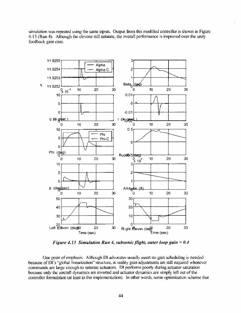
simulation was repeated using the same inputs. Output from this modified controller is shown in Figure
4.13 (Run 4). Although the elevons still saturate, the overall performance is improved over the unity
feedback gain case.
11.9255 t
Alpha [11.9254 Alpha-C
11.9253 v
11.9252
10 .410
10 20 30
5
0 L/
q (de__ ec )0 10
10
2O
I
[_ Phi5/s\ h,Co V
Phi (_d_g)0 10 20
10
30
30
5
oC'- Ap (d_e_rsec)
0 10 20
50,
4o //3o y
2O
30
2
1 /Beta 0 q_)
0
0.01
0 A
-0.01
r (C__dl_ )0
0.5
--.....,
10 20 30
RuddOr5
3
10 20 30
u_El!
x 104 10 20 30
-.---. _
Altit_(l_ (ft_0
30
2o _',
lOi "_ii
0 i
10 20 30
Left Elgvon (degl)0 20 30 Ri ght _evon (de_ 20 30Time (sec) Time (sec)
Figure 4.13 Simulation Run 4, subsonic flight, outer loop gain = 0.4
One point of emphasis: Although DI advocates usually assert no gain scheduling is needed
because of DI's "global linearization" structure, in reality gain adjustments are still required whenever
commands are large enough to saturate actuators. DI performs poorly during actuator saturation
because only the aircraft dynamics are inverted and actuator dynamics are simply left out of the
controller formulation (at least in this implementation). In other words, some optimization scheme that
44

recognizes actuator constraints is needed to overcome saturation problems. This drawback has more todo with the control surface allocation scheme than it does with the DI design itself. However, this result
clearly suggests that the control allocation issue needs to be attacked by treating actuators as nonlinearelements and including them in the DI process. This effort will be handled in a future study.
4.6.4 Uncertainties in Aerodynamic Coefficients
The next issue to be discussed is uncertainty in aerodynamic coefficients. Out of the many
parameters used in the simulation, 13 major aerodynamic coefficients were selected; they are presentedin Table 4.5. The uncertainties are represented as algebraic additions to each parameter, and the
magnitude of the uncertainties is set to three different percentages: 30, 50, and 60. The signs of theseuncertainties, either an addition or a subtraction to/from the nominal values, are randomly chosen andare also shown in Table 4.7.
This set of simulations consists of five runs, one run for each nominal case as well as 30% and
50% uncertainty cases and two runs for the 60% case. The same set of flight conditions (A in Table4.6) is used for all five runs. The same set of command inputs, 10° singlet co,hands for both c_ and 0,
is also applied for each run.The controller used for Runs 5 thorough 8 is the same controller that is used for Runs 1
thorough 3. The controller used for Rtm 4 has the same structure, but the gain of its outer 0-loop isreduced from 1 to 0.4. This modified controller also is used for Run 9.
Run 5 (Figure 4.14) is the nominal case. The vehicle responded well to the con_nanded inputs
and no actuator saturation took place.Run 6 (Figure 4.15) is the 30% uncertainty case. Despite the right elevon saturation at
2 seconds into the simulation, the vehicle still behaved well.
Run 7 (Figure 4.16) is the 50% uncertainty case. The divergence from the nominal case isobvious. Overshoots are large, especially during the period when the elevon saturation occurs. The
bank angle excursion is also large because of pitch axis priority in the control surface managementscheme. The lack of roll control authority under these conditions is underscored in this simulation.
Next, uncertainty is increased to 60% in Run 8 (Figure 4.17). The vehicle obviously diverges
from the nominal trajectory, probably catastrophically.
From the 50% tmcertainty case results, as well as by looking at the right elevon time history in
this case, it is clear that elevon saturation, coupled with the priority for pitch axis control, causes loss of
control. A quick (though not necessarily optimal) solution to this problem is, as in the previous case,
reduction in outer 0-loop gain. This approach is examined in the next simulation run (Figure 4.18).
45

40
35[ /---
AlPhL_5 d_.n_0
10
-- Alpha tAlpha-C
10 20 30
15
/10 20 30
_ Phi
105 _/ l Phi-C
Phi (d_0 10 20 3O
10
p (d_e__ec_0
3O
f10 20 30
1 d__ - _-_-_'----'--_"Beta0
0 10 20 30
0.1
o N_
0 10 20 30
_,_/
0x 1048
10 20 30
7.5 '--- _.._7 "'"_
---__....Altit_d3e fft_
0 10 20 30
40
20b_-- 20
0 0
Left Elevon (deg]0 20 30 Right L_evon (de_) 20Time (sec', Time (sec)
3O
Figure 4.14 Simulation Run 5, supersonic flight (M_ = 2.38)
46
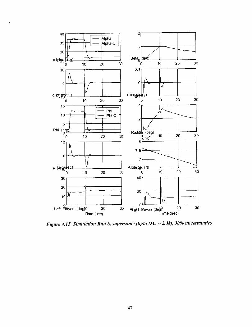
40
351
0
10
t
----,-- _- Alpha t/ Alpha-C
L_10 20 30
2
Beta0 )d_ _-_ _--_
0 10 20 30
q _le_g__ )0
0
10
0.1[
10
o\
V
20 30 10 20 30
[
l Phi-C J
L
o _,
r (de_(_/.,_0
4
Rude'- (de_)
0 104 10
7.5 _
Altit__
0
4O
0 20 30 20 30
(ft_
p (_l_:iec_0 10 20
30
20 _.__.,_,
lo_ I"
0Left EI0von (degl)0 20
Time (sec)
30 10 20 30
0
30 Right I.Blevon (de_ 20 30Time (sec)
Figure 4.15 Simulation Run 6, supersonic flight (M. = 2.38), 30% uncertainties
47

EA'°haIAlpha-C
10 20 30
0
20
10 20 30
p (cle__g_,,_ec _0
30
20
0
3O
0 20 30
Left Elgvon (degl)O 20 30
Time (sec)
0
4
2O
/
Rud_ i- (deu)
0x 10_ 108
3O
10 20 30
20 30
7.5
7
Altit_d_0
4O
----.....(ft/
10 20 30
o LRight LBlevon (de_ 20 30
Time (sec)
Figure 4.16 Simulation Run 7, supersonic.flight (M_ = 2.38), 50% uncertainties
By using the controller from Run 4 with the outer 0-loop gain reduced from 1.0 to 0.4,
simulation Run 8 was repeated as Run 9. With this change in gain, the vehicle readily recovers from the
upset, which suggests that gain modifications are effective in alleviating actuator saturation. Certainly the
complexity of the controller increases as the number of gain alterations increases. There is, therefore, a
tradeoff that designers have to consider between controller complexity and perfomaance of the
controller for the best controller design.
48

200
100
0 \
0
50
/V
0 ..fN
0
400
200 _-
10 20 30
/
0
Phi __0
20O
10 20 30
100
0 "'" --
0
5O
m_
Phi
-- Phi-C
10 20 30
10 20
/30
0
-50Le_ El_on (deg_0 20
Time (sec)
L
5
0
-5
Beta _ _q)0
4
2
0 "-
J
\10 20 30
r (de_{seci
0 10
2O
0 ---"-----"
-20
Ruder8 deg)0 10X 104
7'if
Altit_.d_.
20 30
0
5O
2O 30
(ft_
10 2O 3O
_ ght _,von (deg_0 20 30Time (sec)
Figure 4.17 Simulation Run 8, superxonic.]light (M_ = 2.38), 60% uncertainties
49

4O
3O
AI ,r'_n_0
10
| ,
AlphaIAlpha-C
10 20 30
3O
3O
0 20 30
1
0.5 /
Beta (_0 10
0.1
r (de_(_/.,_ ,_0
4
2yRud&2 (d_u)
Ux 10 4
8
2O 30
10 2O 3O
0 20 30
7.5 """
7 ""'-Altit_ (ft_
0 10 20 30
4O
2O
'i olLeft Elevon (deg)0 20 30 Right lSlevon (del_ 20
Time (sec) Time (sec)
3O
Figure 4.18 Simulation Run 9, supersonic flight (M. = 2.38), 60% uncertainties,
outer _-loop gain = 0.4
4.6.5 External Disturbances Effect: Side Gust
The final simulation example is an external disturbance case. We chose a side gust as a
representative case of such disturbances and their effect on DI controllers. The gust input shown in the
upper left comer in Figure 4.19, Run 10, was added to the body y-axis velocity of the vehicle. The gustreaches up to 50 ft/sec, and the overall duration of the gust is 4 seconds. The flight condition used is the
subsonic case (M= = 0.63), Flight Condition C, shown in the Table 4.6.
5O

The side gust disturbance input produces a maximum sideslip angle of about 1% Also, bank
angle is excited up to about 12° because of yaw-roll coupling. Bank angle did damp out rapidly (after
approximately 1 cycle), and the sideslip angle became essentially negligible roughly 10 seconds after thegust was introduced. Overall, this DI controller worked well for rejecting external disturbances.
60
20
0
Side__ ;t (ft/sec_
0
2O
10
0
Phi (_:
-20010 20 30 10 20 30
1.5
1
0.5
-0.50 10 20 30
20
10
0
pid49 -20
0 0 20 30
0.4
O2oJ\r (dC_/s2e :
-0.40 10 20 30
50
40A30 _
Left_2 , J_(de_ -
0 10 2O 3O
0.4
0.2
0
-0.2Rudder (c eg)
-0.40
3O
20
10
I_ ght
010 20 30 10 20
Time (sec) Time (sec)
Figure 4.19 Simulation Run 10, subsonic flight (M. = 0.63),external disturbance: side gust
3O
51

4.7 Design Example 2
4.7.1 Introduction
Even in instances where the control input matrix g(x) shown in Equation (3.4) is invertible,problems will arise if the matrix is very small in magnitude, indicating reduced control effectiveness on
the state dynamics. Should this occur, the control becomes unbounded, causing actuator saturation.For example, a control ineffectiveness problem is typically encountered in the inversion of angle-of-
attack dynamics because the vehicle's longitudinal control surface has little effect on the angle-of-attack
rate. A 2-time scale method has been developed and applied in previous research to bypass thisproblem. _7.ts In our method, the control surface is used to generate the pitch rate dynamics, _,
directly. The resulting pitch rate is then used to control _. Figure 4.20 illustrates this approach in which
two DI loops are present: a fast inner-loop inversion for rotational rate variables, such as q, and a slow
outer-loop inversion for rotational variables, such as _.
_cmd qcmd _e,cmd
Plant and 1
Slow _ Fast I Actuator /
Inversion lnvorcicm I Dynamics _ q
-'" , " " vc_r_iOll " • ,, ,, w • •Fig e 4.20 2 ume ule oj angle-Oj-uHuctt uyautalc:
Equation (4.16) shows the pitch rate command generated by the slow outer-loop inversion, andEquation (4.17) shows the devon command generated by the fast inner-loop inversion, required to
produce the desired angle-of-attack response. It should be noted that both control laws require angle-
of-attack and pitch rate feedback, which is full-state feedback for the short period approximation.
I+uZ q,) (4.16)
8_.cmo :Ma'(_-M_O_-Mqq) (4.17)
The control laws shown above are used to invert the inherent pitch rate dynamics and the angle-of-
attack dynamics, respectively. The proposed forms of desired dynamics developed in Section 3.6 are
applied separately to each of the short-period state dynamics before they are evaluated in terms of
• Time domain performance,
• Stability robustness and performance robustness,• Effect on motion sickness,
• Quadratic cost function, and
• Passenger ride comfort index.
52

4.7.2 Time Domain Design Requirements
The time domain performance specifications used to evaluate vehicle response are short-period
damping ratio and natural frequency. The requirements for the X-38 vehicle are selected from Mil-STD- 1797A _4to satisfy Level I flying qualities for a Class 11vehicle during a Category B flight phase.These Level 1 standards bound the short-period damping ratio and natural frequency as follows:
0.30_<4< 2.0 (4.18)
0.7s -_ < co,, < 1.3s u (4.19)
The time domain response requirements lbr a step input are shown pictorially in Figure 4.21. These
requirements satisfy Level 1 flying qualities for the vehicle.
K4
K3
K2rrID
7_
> K1-tD
t_
OZ
,./........ ,..///.%," ,...,.,... /.//..,
I_'.-,-.., ,. ,,,,/,, ,./,- ; ,/./,...;..,I "_._.'/l'l//./..'///. t'!1 t
--_"_}(11'/,/11/////,.: I,
I Il---.-I---
-----._J..',.'i,._"i'4 .l///141/i///#_,'W(,7"/J tl//liJ/'."./l/_;;..-;,',i ",......."',#/,<.'-.'/,';
/_.l_,;/,./.,.;..;_d ///, /,+/, ."t/,,. _, J ,*ea l y ,' t i " i +_ >l l ,, J , _p/.I._il ..'.,**_l_l./;;:.;:i',;;. :,:,,.,,"
___..{i],'_ "ll,/ i'IA/ i'/'/li"l_,','].'," )/71 / 1/" ,'A i , .,I i ,."I_AL',;,'; "'"" ",,r, ..... ,,v,.
__:7">'_ .'"/, "4" , ""/," .;l! .:' Ijl"" "/ i/X/l" i ."ll)"t Ii'i'lii/i.I/I./__,'.3_.,., ........,._,....,,.,y,
I_'/./,2",:_.,/," ,:/,_.,4-'.--'./4"11+_/../,. ;.,,q,.",'I..-/,i,,//,",.-'
_, ,'_ ;-./.-;.""./.4";'!":-"]'"" """_"_
0 T1 T2 T3 T4 T5Time (seconds)
T6
Amplitude
ComJnand K 1 K2 K3 K4
Alpha to 2.0 ° 0.63 0.9 1.1 i.2
Roll to 10° for 0.63 0.9 1.1 1.2Mach < 1.0
Roll to 10° tbr 0.63 0.9 1.1 1.2Mach = 1.0
Command T I T2
Alpha to 2.0 ° 1.0 3.0
Roll to 10° for 0.5 1.25
Mach < 1.0
Roll to 10° for 0.75 3.5Mach = 1.0
Time
T3 T4 T5 T6
3.0 4.5 4.5 6.0
2.0 3.0 4.0 4.5
5.25 6.0 5.25 10.0
Figure 4.21 Time domain pelJbrmance .specifications
53

Two numericindicesarealsousedtoevaluatetheresponsesof eachcontroller.A quadraticcostfunction,J,(showninEquation(4.20))isusedto evaluatethemagnitudeof eachcontrollerresponsein termsof thefour longitudinalstatesandtheelevoninput.
J = xVQx+ ulRu (4.20)
It was desired to weight angle-of-attack more heavily than pitch rate because angle-of-attack is the
variable being controlled. Since the behavior of the phugoid mode is less important, the velocity and
pitch attitude states are weighted less than the short period states. Therefore, the weighting matrices
usedare: Q=diag(.1 10 1 .1) and R =1. A passenger ride comfort index_ 9, shown in Equation
(4.21 ), was also used to evaluate the responses.
C = 2.1+ 17.2g, (4.21)
The RMS vertical acceleration, R_, is a, = U 0&- U,, cos (o%) q + gsin ( 0r, )0 in which vertical
acceleration subscripts denote trim values. Lower comfort indices indicate increased passenger ride
comfort.
4.7.3 Controller Design
The proportional, PI, and flying qualities dynamics desired are selected to satisfy Equations
(4.18) and (4.19). The ride qualities dynamics were selected to satisfy the desired CAP and damping
ratio values shown in Figure 3.13. Table 4.8 summarizes the desired dynamics selected for these
controllers. Each set of dynamics acts on the error between CV corr_and and its feedback tenn. Therobust outer loop was designed via pole placement through the use of MATLAB's place command.
This outer loop consists of full-state feedback that is operated on by a matrix of gain values. The poles
were placed according to the desired closed-loop pole locations.
Table 4. 8 Desired Dynamics Selection
Angle-of-Attack CaseDesired Dynamics Slow inversion Fast Inversion
Proportional 0.8 1.3
Proportional
Integral
Flying Qualities
Ride Qualities
+ 6.25 (CV_,,,a -CV)
1.4(s+0.8)2s + 2.24s + 1.96
1.96
s+3
1.5(S+0.8)2s + 2.24s + 1.96
7
s+4
54
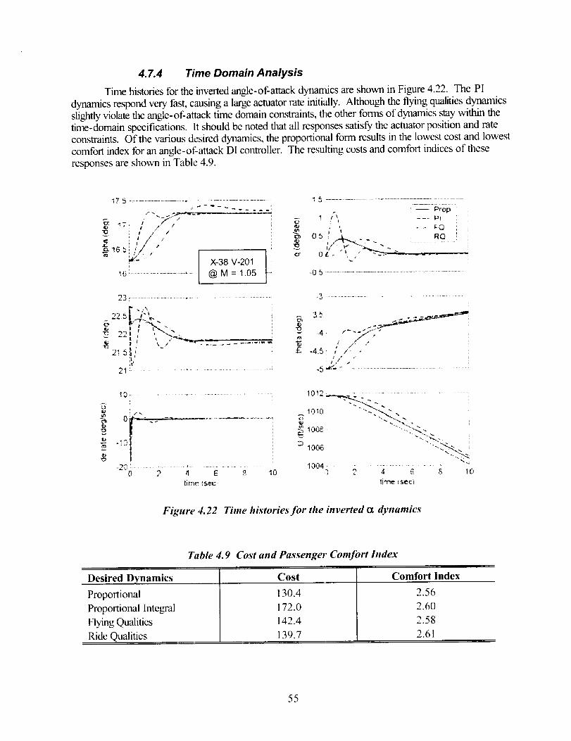
4.7.4 Time Domain Analysis
Time histories for the inverted angle-of-attack dynamics are shown in Figure 4.22. The PI
dynamics respond very fast, causing a large actuator rate initially. Although the flying qualities dynamics
slightly violate the angle-of-attack time domain constraints, the other forms of dynamics stay within thetime-domain specifications. It should be noted that all responses satisfy the actuator position and rate
constraints. Of the various desired dynamics, the proportional form results in the lowest cost and lowest
comfort index for an angle-of-attack DI controller. The resulting costs and comfort indices of these
responses are shown in Table 4.9.
175 ........................................._ ..................................................
:7: / i13 i t ./- /
_/-" I X-38 V-201 I_,_ .................................. @ M = 1.05 -'
23 r ..................... • ..........................
2! 5!/t _
21 .............................................................................
e-,
fcrl
#3
£
3.6 , . _,. !
45! is. ,": ' • ,," i
#',Z ,:
1012 ..........................................
_ 1008, _-_
lOO6, '- 7%- ..
1004 .................................. "' _ _ 6 & 10
time _eci
Figure 4.22 Time histories for the inverted o_ dynamics
Table 4. 9 Cost and Passenger ComJbrt Index
Desired Dynamics
Proportional
Proportional Integral
Flying Qualities
Ride Qualities
Cost
130.4
172.0
142.4
139.7
Comfort Index
2.56
2.60
2.58
2.61
55

4.7.5 Frequency Domain Analysis
Robustness is a key element in the reentry vehicle flight control system design because of thebroad flight envelope in which these vehicles must operate. The robustness technique that is used to
analyze controllers developed in this work is adapted from current research in robustness methods for
the X-38 vehicle 2°. A sigma-Bode plot of the loop gain singular values is used to evaluate robustness
over a range of input frequencies. Further explanation of the sigma-Bode plot can be found in Section4.8.2. The performance and robustness criteria used to evaluate the controllers in this section are
• Zero steady-state error.
• Attenuation of low-_quency disturbances by a factor of 0.1.
• Linear model accuracy to within 10% of actual plant for frequencies up to 2 rad/sec and growthwithout bound at 20 dB/decade thereafter.
To satisfy these requirements, illustrated in Figure 4.23, the singular values of the loop gain must lie
outside of the performance requirement and stability requirement areas for all frequencies.
2gO
t -50
0
PerformanceRobustness
_, Requirement
Motion
Sic kness
Range
-1(_3 ........... ............... .........10 1_ !'3 lq 113 lf_
Figure 4.23 Robustness constraints
An additional requirement on signal attenuation can be added to the singular value plot of Figure4.23. For this example, attenuate the signals between 0.6 rad/sec to 1.6 rad/sec in order to alleviate thepassenger motion sickness that can occur at this frequency range J'_. Since the singular values of a matrix
represent the relative size of a mode, attenuate the singular value response within this frequency range.
The singular value response within this range should be continuously decreasing. Any amplificationwithin it would increase the passengers' motion sickness.
The sigma-Bode plots for these cases are shown in Figure 4.24. Both the proportional and the
PI desired dynamics violate the stability robustness requirement above 20 rad/sec. These dynamics alsoviolate the attenuation requirement toward the higher end of the frequency range. Figure 4.24 clearly
indicates that flying qualities compensation and ride quality compensation are sufficient for a robust
angle-of-attack D! controller because they satisfy stability robustness, performance robustness, and the
56

motion sickness constraint. Table 4.10 summarizes the results of each set of desired dynamics in terms
of satisfying time domain and frequency domain requirements.
: ...... Prop=:!. i ...... PI !
b i
........ FQ, ,: ...........RQ i
i, ii_
il _ !i
Figure 4.24 Sigma-Bode of closed-loop ,_ystem
Table 4.10 Summary of Compliance with Design Specifications
Desired Dynamics
Proportional
PI
Flying Qualities
Ride Qualities
Control
Responses
Step
Response
3
3
3
3
Robustness
Constraints
Motion
Sickness
5
5
3
3
4.8 Design Example 3
4.8.1 Introduction
A systematic way to synthesize and analyze the robustness of a Dl-based controller
hi a straightforward manner must be found _ that engineering intuition can be easily applied throughout
57
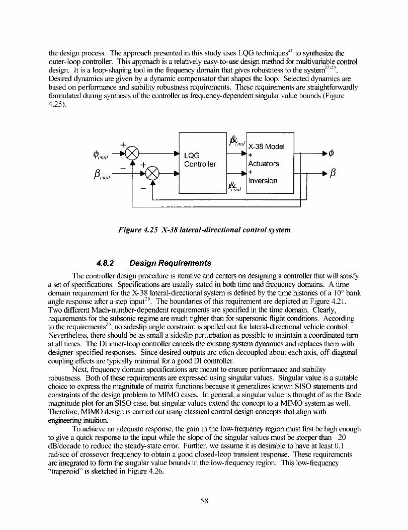
the design process. The approach presented in this study uses LQG techniques 21to synthesize the
outer-loop controller. This approach is a relatively easy-to-use design method for multivariable control
design. It is a loop-shaping tool in the frequency domain that gives robustness to the system 2225.
Desired dynamics are given by a dynamic compensator that shapes the loop. Selected dynamics are
based on performance and stability robustness requirements. These requirements are straightforwardlyformulated during synthesis of the controller as frequency-dependent singular value bounds (Fignre4.25).
_cmd
LQGController
X-38 Model+
Actuators+
Inversion IFigure 4.25 X-38 lateral-directional control ,wstem
4.8.2 Design Requirements
The controller design procedure is iterative and centers on designing a controller that will satisfya set of specifications. Specifications are usually stated in both time and frequency domains. A time
domain requirement for the X-38 lateral-directional system is defined by the time histories of a 10° bankangle response after a step input 26. The boundaries of this requirement are depicted in Figure 4.21.
Two different Mach-number-dependent requirements are specified in the time domain. Clearly,
requirements for the subsonic regime are much tighter than for supersonic flight conditions. Accordingto the requirements 20, no sideslip angle constraint is spelled out for lateral-directional vehicle control.
Nevertheless, there should be as small a sideslip perturbation as possible to maintain a coordinated turn
at all times. The DI inner-loop controller cancels the existing system dynamics and replaces them with
designer-specified responses. Since desired outputs are often decoupled about each axis, off-diagonal
coupling effects are typically minimal for a good DI controller.Next, frequency domain specifications are meant to ensure performance and stability
robustness. Both of these requirements are expressed using singular values. Singular value is a suitable
choice to express the magnitude of matrix functions because it generalizes known SISO statements andconstraints of the design problem to MIMO cases. In general, a singular value is thought of as the Bode
magnitude plot for an SISO case, but singular values extend the concept to a MIMO system as well.Therefore, MIMO design is carried out using classical control design concepts that align with
engineering intuition.
To achieve an adequate response, the gain in the low-frequency region must first be high enough
to give a quick response to the input while the slope of the singular values must be steeper than -20dB/decade to reduce the steady-state error. Further, we assume it is desirable to have at least 0.1
rad/sec of crossover frequency to obtain a good closed-loop transient response. These requirements
are integrated to form the singular value bounds in the low-frequency region. This low-frequency"trapezoid" is sketched in Figure 4.26.
58

m
00
>
t_
o_¢.-
CO
200
150
100
5O
....... i ....... i ....... i ....... i .......
.i-a
E
High gain at low frequency for _ _ '-'w
/7 fast response _ _ _"//// -20 dB/decade to reduce
_ steady-state error
-""__ I_ Minimum crossover
_'_f_- frequencyPerformance I Low gain at high frequency for
Requirement[dist,....,_, ,, ......, ,urbance..r,eje,ction ...............-50
10 .3 10 .2 10.1 10 ° 101 10 _
Frequency (rad/sec)
Figure 4.26 Frequency domain requirements
At high frequencies, singular values are bounded by the unmodeled dynamics associated with
high-frequency models such as flexible and vibrational models. These high-frequency models are often
neglected when the plant model is being developed; the vehicle is often treated as a rigid body. As a
result, there is a difference between the assumed mathematical plant, G DC, and the actual plant, G']_.
This difference is defined and described as model uncertainty 27. Here, an unmodeled dynamics model,
suggested by Stevens and Lewis 27, is used. This uncertainls, model assumes tile rigid body model is
accurate to within 10% and up to a frequency of 2 rad/sec, after which the uncertainty grows at a rate
of 20 dB/decade. This uncertainty model is expressed in the following transfer function and is used to
model the uncertainties of the X-38 vehicle at high frequencies:
mbg s+22-0 (4.22)
We assume m[_( to be bounded with uncertainty in the X-38 vehicle transfer ftulction. Multiplicative
uncertainty is expr_essed in terms of an assumed plant model and the actual plant by
'l o,g[,+ g; oc,
where the unknown discrepancy satisfies a known bound.
59

Under this assumption, for stability robustness with modeling errors, the loop gain referred to the outputshould satisfy:
when l/m[_g:< 1. Here, K represents the compensator. This uncertainty bound, which is obtained
from the unmodeled dynamics, is applied in the high-frequency region. Finally, the complete frequency
domain bounds are shown in Figure 4.26 (previous page).
4.8.3 Lateral-Directional Dynamic Inversion Controller
Lateral-directional DI control equations were developed previously in Section 3.2.2. The
following form, which is provided in Equation (3.12), is used for this example:
Fp-l"'<'<"[(4.26)
4.8.4 Dynamic Inversion Inner-Loop Controller
The lateral-directional D1 controller, together with the X-38 model and control surface blocks,
forms the DI inner-loop augmented system. This augmented inner loop is
_7. = A/I.x/I. + BuU/L, (4.27)
where the inner-loop state vector, x_z , is
xzc =[,6 p r 0 6a_ 6a _5_& _,']' (4.28)
and the inner-loop control vector, uH_, is
The state matrix,
are expressed numerically as follows:
(4.29)
Azt" , and the control distribution matrix, Bt_ for transonic flight (Table 4.5, Case B)
60

- 7.8e- 2 0 -1.0 4.9e-2 0 0 0 1.5e-2
-3.1e +1 - 2.3e-1 2.5e- 1 0 0 3.1 0 9.3
4.0e- 1 2.2e- 2 -9.8e- 2 0 0 - 8.5e- 3 0 -1.5
0 1 0 0 (} 0 0 0
A,. = 6.3e+3 1.9e+l 8.3e+1 0 -3.7e+1 -6.8e+2 0 0
0 0 0 0 1 0 0 0
1.5e+ 2 1.0e+! -4.6e + 1 0 0 0 -3.7e +1 - 6.8e+
0 0 0 0 0 0 1 0
EOoOOO2_+_o,30o1_B;£= 0 0 0 1.4e+3 0 -4.7e+2
We assume measurernents are limited to bank angle, 0, and to sideslip angle, [3. Therefore, the
following output equation results are:
[:][ooo,ooooI= Xll"Y 0 0 0 0 0 0 0
The block diagram representation of this DI inner-loop is shown in Figure 4.27. In addition, the singularvalues of the inner-loop versus frequency are plotted in Fig_Lre4.28.
DI Inner Loop
i Inversion _, Control_,, Surfaces
t cmd
)(-38Model I ', _ y
I...............................................
Figure 4.2 7 Dynamic Inversion Control Inner-Loop block diagram
61

rn
if)
>
I
c-.I
CO
200
150
100
5O
-5010 -3
....... i ....... |
X-38V-201 l@ M = 1.05
__ / Upper Bound
i i
10 .2 10 -1 10 ° 101 102
Frequency (rad/sec)
Figure 4.28 Singular values of the dynamic inversion inner-loop ,_ystem
4.8.5 Augmented System
Since DI alone does not achieve the desired specifications, stability robustness requirements at
high frequencies are not met. Integrators are added to each control channel to correct this deficiency.
The X-38 plant, actuators, and DI controller are au_nented to form the following system:
where
and
_.,,,_= A,.,_x,,,,,. + B ,,,,,u.,,,. (4.31)
x,,,,.. =[,B p r O g_ _a &_ N" eo e#] r (4.32)
(4.33)
62

In Equation (4.32), e0 and e, are augmented states because of the addition of the integrators in the
bank angle and the sideslip channels, respectively. The augmented matrices, A,,,_, and B,,,,_, are
obtained by performing the following manipulations:
A,,,,,; = L o ;- and B,,.:, = 1:(4.34)
The corresponding singular value plot for this augmented system is shown in Figure 4.29. It suggeststhat the nominal design has now been reshaped to meet the specified frequency domain requirements.But we still have not tailored the outer loop for robustness, and we have not dealt with the LQR-LQG
observer issue.
rn
q_
ID
>
"5
t"-
09
2°°1........ ' ......... ' ................. I ......./ x-38v-2ol I
_- IL _ Upper Bound I
t2_-50 _
-IO0 -
..... i ........ i ........-150 : : " ''"'
10 3 10 _ 10 _ 10 ° 10 _
Frequency (rad/sec)
Figure 4.29 Augmented system singular values
4.8.6 Observer Design
The objective of this step is to create a fast dynamics observer that can be used with a regulator
to form an LQG controller that will satisfy both performance and stability robustness requirements. The
form of the observer is a Kalman filter designed for the augnnented system of the previous section. The
following weighting matrices were selected, by trial and error, so that the singular values of the resulting
Kalman filter open-loop gain, CF (s)L, satisfy the singular value frequency domain requirements:
63

Q = diag (1,
where F (s)= (sl- A)-'.
1, 1, 1, 1, 1, 1, 1, 1xl08, 1xl08) and R = 0.0051_
The resulting Kalman filter gain is given by
=[-5.1e-l| 2.6e+I 8.7e-1 1.6e+l 1.4e+l 1.9 2.6 -8.3e-1 1.4e+lL L 1.6e+l -I.6e+l -2.5e+1 -5.1e-1 1.4e+3 6.9e+1 -3.2e+2 1.8 5.1e-I
and the corresponding Kalman filter poles are
s =-18.4 +__18.4,- 18.4+18.5,- 14.1 + 0.72,-0.86 + 0.50,- 0.87 +0.49.
_ _T
.t_-1 /-l.4e+t.J
4.8. 7 Regulator Design
A regulator is designed next, assuming full-state feedback. The resulting regulator is combined
with the Kalman filter from the previous step to form an LQG controller for the system. The regulator is
based on LQR methodology, and the following weighting matrices are selected for tl_ LQR gaincalculations so that the corresponding LQG singular value plot (Figure 4.30) satisfies the singular-value
frequency domain requirements:
Q =dia_(1,1,1,1,1,1,1,1,1xlOS,lxlO _) and R =!,
Or)
>
¢-
200
r-150 / X-38 V-201
[ @ M = 1.05 Upper Bound
100 _'___"'_ Lower Bound
-50 _
-100
-150
-200 ........................ ' ..........
10 3 10 .2 10 1 100 10 _
Frequency (rad/sec)
Figure 4.30 Singular values of the LQG regulator
64

The resulting regulator gain is as follows:
K= le-2 1.2 3.5e+1 -1.1e-I -4.3e-3 -2.1e-1 -4._-2 -1.5 1.7e-4 1.0e+4J (4.35)
For the LQG singular value plot, the complete dynamics are given by the following augmented system:
A-LC-BK
y_- co(:](4.36)
with transfer function CF (s)BKF ,. (s)L. The singular values are plotted in Figure 4.30. The singular
values of the resulting system clearly meet frequency domain specifications at all frequencies of interest.
4.8.8 Time Domain Analysis
Once the controller is desigmed to meet the frequency domain specification, its performance
must be tested in the time don_iin against the time-domain specification (Figure 4.21 ). Figure 4.31shows the response to a 10° bank angle step input to the system as defined in Equation (4.36). The
bank angle response is within the design envelope while the sideslip angle is negligible. Also, both
control surfaces are relatively inactive, and both displacement and rate are within the limits for eachsurface. The controller design, therefore, ,satisfies time-domain specifications at this stage.
4.8.9 Gain Schedufing Issues
As previously discussed, the main advantage over classical methods for the D! design
methodologw is the little need associated with the DI design |nethodology to schedule gains. In order toverify this claim, the designed controller, which is tuned at the transonic flight condition (Table 4.5, Case
B), is applied to other flight conditions (Table 4.5, Cases A and C) without modification. The other two
flight conditions, subsonic and supersonic, illustrate this analysis. The same 10° bank angle step inputsare applied to all three cases, and the resulting responses are presented in Figure 4.32 for the subsonic
and transonic flight condition cases.
65

t-O
15
10
5
0
-50
10
-50
-*.,,.w,.,
l_ p.i(deQ)
................................................................!...........I I i I I l f I I
2 4 6 8 10 12 14 16 18
_ da (deg) i....... da-rate/deg/sec)
i t i a i | I I I
2 4 6 8 10 12 14 16 18 2
"0"0
1
0.5
0
-0.5
-1
-1.50
• ' ....... " _ " " I '_- dr (deg) ' I
-. . .:""/ ....... ............. _ ....... dr-rate (de,q/sec) J
Ii i i | | I | I i
2 4 6 8 10 12 14 16 18 20
time (sec)
Figure 4.31 10 ° bank angle step response
66

20:
(1) , i, 6" %
-=--- "- "._ P'q,. _ J'',l,,./
Q..
00 5
5
0 _L
........"ID
10 15 20
-50 5 10 15
"G" 10
5"t3
L0 ""_
"%, .........-o -5
0 5 10 15
Figure 4.32
20
20
time (sec)
0.5
o°_ %_
0 ;\ .._- . ......,+..,
c'_
-0.50 5 10 15 20
-B -1 I
X-38 V-201-2 T
0 5 10 15 20
"G" 1
0kd _ "'',_ -------'ID
-1 transonic
d.-o -2
0 5 10 15 2O
time (sec)
10 ° bank angle step re.wonse for different flight conditions
In the transonic and subsonic cases, the designed controller is able to stabilize the system. However, it
fails to stabilize the system for the supersonic flight condition. In transonic and subsonic flight, controlsurface activities are well below the limits in rates and displacement. Though the objective of the Dl
controller is to produce a desired response at all flight conditions, no constraints are imposed on controlsurface activities in the DI control equation to achieve this. Control surface deflections and rates are
based solely on the control distribution matrix. In order to avoid actuator saturation, the DI controllermust command no more deflection or rate than the system hardware can provide or the system
becomes nonlinear and the linear analysis may break down. But, these constraints overly restrict the
available control power in some cases. Since a controller selected with this process may not produce
the "best" performance at all flight conditions, the "nominal" (design) condition must be selectedcarefully to achieve good performance in a wide range of flight conditions. Moreover, the specification
will change for different flight conditions. For example, the time-domain specification changes drastically
near Mach = 1. Changing requirements for the entire flight envelope must be considered during thedesign process. The proposed approach allows an engineer to address this issue rather intuitively.
67

5 Robustness Analysis
5.1 _-Analysis Applied to the X-38
5.1.1 Introduction
ha the introductory sections of this document, singular-value decomposition is mertioned as themost common approach to adding robustness to a DI controller design. But it should be again
emphasized that/a-analysis is by no means the only way to tackle robustness issues with this flight
control design. Dang Vu 28suggests that combined techniques using linear quadratic design, quantitative
feedback theory, Lyapunov synthesis, adaptive control, and differential games have all been initiatedtogether with 1a-analysis.
5.1.2 Robustness Example: Application to the X-38 Lateral-Directional Aircraft Equations of Motion
The linear fractional transformation (LFT) structure - spelled out in detail in Section 6.2 of this
document - is now applied to the lateral directional aircraft dynamics for the X-38. First, the lateral-
directional aircraft equations of motion are represented as follows:
[iv0
vr vr
Lff Lp
N_ Np
0 1
V Vpl
Lr 0 +r
mr 0_OJ
0 0
0 %vr
L8 a L8r
N8 a N8 r
0 0
(5.1)
Next, we assume that - except for Lp, La_, N,., and N_.- all parameters are certain values. We also
know the variations (boundaries of uncertainty) for these parameters, too; and we will write them in the
following form:
Lp <Lp <L;
L-6a<-L6a <-L+6a(5.2)
N r <-N r <N +
N_r < NSr < N +-- -- _)r
These bounded uncertainties are now integrated into the aircraft equations of motion using the LFTform. Compare the decoupled roll axis equation
Lpp + LSa8a (5.3)
y=p
68

with the general expression in Equation (6.8). Then, the following correspondences are clearly found:
x=p
U = _)a
a=Lp
b = L_)a
(5.4)
Now, ensure the state space representation of the roll axis eqation with bounded uncertainties in L¢, and
L_, is written by substituting the preceding relationship into Equation (6.13).
[1Zl _
Z2 -
P
" l n°m k / Ln°m-'-P kPl Pl 6a
1 kp2 0 0
0 0 k / 1P2
1 0 0 0
[P
Vl
v2(5.5)
with
kpl -
k / =Pl
_(c_a .nomI_nomP2
Similarly, yaw axis aircraft equation
t&= Nrr + NSr5 r
y=r
is put into state space form with uncertainties in N,. and N_.
, Nno mljlN n°m krl k /
[zl] l ri rl 6rE
z3 = _'2 0 v 3
0 k / v4
r2 5r0 0
with
(5.6)
(5.7)
69

--- , kr2=kr, (Nt-N -I
- "r )- 2" r°n'
2'N+ -Nn°mt[Ik ,Om (N + ) 2N n°mk / = , 8r _r ]_ ir - N_ ) k/ = _ - N_r - 5r
r, (N8+- N-_5r } r2 (NS+r - N_r )
lnte_p-ating both roll and yaw axis equations with Equation (5.1) yields the following LFT form for thelateral-directional equations:
-- --9
gq
15¢1
Zl
Z2
[z3
Z 4
P
r
iO
VT VT VT
= L[j Lp Lr
Nf_ Np Nr
0 1 0
-0 1 0
0 0 0
0 0 1
0 0 0
1 0 0
0 1 0
0 0 1
0 0 0
0 +
o _¢J0
O kp2
0 0
o -f_q o
0 Pl+ 0
0 *''
00 01
00
0I
0
0 Y_'VT
L6a L6 r
N6 a N6 r
0 0
0
0
kr 2
0
0
0
0
0
0 0 0 O
k / 0 1 0P2
0 0 0 0
0 k / 0 1r2
0 0 0 0
0 0 0 0
0 0 0 0
0 0 0 0
Vl
v2
v3
V4
8a
_r
(5.8)
5.2.
The input/output description of the plant and the uncertainty block are shown in Figures 5.1 and
V 1 _1_
V2
V3 •V4
5a
G
Z1
Z2
z3
._____ Z4
---_ yr
Figure 5.1 Piant input/output
70

Z1 --
Z2_
Z3--
z4_
p F81 0 0
I_ I0 82 0
_lO 053IP ,
[0 0 0
0 L---_v_
0 _--_v2
i
Figure 5.2 Uncertainty block
These two blocks are interconnected to form a Parametric Uncertainty block, as shown in Figure 5.3.
j3_
pd !I
r4
f/
Plant"ql
.¢I/
Perturbed Model
6r
Figure 5.3 Aircraft plant with paranletric uncertainty
Parametric uncertainties are not the only type of uncertainties to be considered in this example.
As discussed in Section 6.2.2.1, unmodeled dynamics or uncertainty at the input is another important
type of uncertainty to be examined. When this is applied to our case study, the following weighting
function, W,,, is used. Its place in the lateral-directional block diagram is shown in Figure 5.4.
. s+l 1
0
Wi n = S +'100S+I
o s- 5oj
(5.9)
71

elevoncmd
ruddercmd
Figure 5.4 Unmodeled lateral-directional aircra]t dynamics
10o
"0
10 -I,__r"O_
=E
10 -2
10 -1
/./.'
./'
//
./
,//
/./
//Y
JJ
10 0 101 10 2 10 _
Frequency (radlsec)
Figure 5. 5 Uncertainty weigh ring function
This particular uncertainty weight, W,-,,,indicates that there is potentially 1% modeling error at
low frequency and that the uncertainty in the model grows up to 100% at high frequency. The
uncertainty weight is diagonal in form with equal diagonal elements. The perturbation mode is a circle,
or a sphere, around the nominal plant.A third type of uncertainty, discussed in Section 6.2.2.2, is uncertainty at the output (uncertainty
in the measurements used) in the feedback loop. For our lateral-directional example, Figure 5.6 shows
a block diagram representing the treatment of this type of uncertainty. Since it is unstructured, it is afunction of input frequency - as was the uncertainty at the input.
_eas 4 /3
Pmeas _I Prmeas _ r
noise
Figure 5. 6 Unstructured uncertainty at the plant input due to output uncertainty
72

100 . , , ,
10 -1"0
_-" 0-2"2 1
10-3
-4
f
10 -3 10 -2 10 -1 10 0 10 I
Frequency (radlsec)
Figure 5. 7 Unstructured output uncertainty weight
This output uncertainty weighing function implies in p and r a low-frequency measurement error of
0.003 rad/sec and a high-frequency measurement error of 0.015 rad/sec. The model of measured value
of p, denoted p,,,,.,,,, is given by
Pmeas = P + Wnp qp , (5.10)
where By is an arbitrary signal with
Any type of controller could be used in conjunction with our DI controller for pt-analysis. Muchof the literature favors an H_ controller that can provide the robusmess sought through p.-analysis -
largely because g-synthesis, which is an extended and more complex form ofla-analysis, requires an H_controller combined with _t-analysis to synthesize an optimized controller to achieve stability
performance. In our example, an H_ controller is designed using the MATLAB p.-Analysis andSynthesis toolbox _ .
The objective of the [l_ controller is to make the pitch and yaw rate of a vehicle closely follow
the commanded values of these two parameters (i.e., the goal is to minimize the errors ep and ez,).
Frequency-dependent weights are connected into the structure as shown in Figure 5.8.
Pactual'__ I----'--I
Pcmd_'_l_ ep
ractual-_-__
rcmd_I_W[W_-_ er
Figure 5. 8 PerJbrmance Weighting block diagram
73

Theoverallperformanceerrorvectorisgivenby
eperf = Ee l=ts:l m -Oac,ua,er s + 10 L rcmd FactualS+I
The shape of the weighting function (Figure 5.9) is chosen so that the controller providesperformance in the low- to mid-frequency range. Error weights on the roll and yaw rates indicate a
tolerance of 0.1 rad/sec at low frequency and 1 rad/sec at high frequency.
(5.12)
O"O
¢-
t U
¢10 r
10" _ D"__tG'_ 10'
Frequency (rad/sec)
Figure 5. 9 Performance weighting as a function of fi'equency
Limits on the actuator deflection magnitude and rates are also included in this example through
W_c, (actuator weight) shown in Figure 5.10. This mathematical constraint is not a physical "limit" but is
treated as a constant weight matrix to produce the "error at the actuator" e_,c,.
rudder__
m
W_t _ eac t
Figure 5.10 Control Surface Actuator Weights block diagram
This error vector is defined as
74

eac t = Wac t
- _elevon
Oelevon
t_rudder
O rudder
with Wac t =
10 0 0
5O
10 0 0
22.5
10 0 _ 0
50
0 0 0 125
(5.13)
The two types of perfomaance weights just described are combined to form a closed-loop weighted
performance transfer matrix as shown in Figure 5.11.
Pcomrnand --'_
rcommand vb"
Psensor no,se _-.
/'sensor noise _-.
Closed-loopWeighted
PerformanceTransfer
Matrix
_elevon error
_.- _elevon error
_rudder error
_rudder error
_- rerror
,_ Perror
Figure 5.11 Weighted perJbrmance objective tran._['er matrix
Next, an H_ controller is designed to minimize the tt_ norm of the nominal closed-loop transferfunction from the disturbances to the errors. This design is actually a sub-optimal H, controller because
the controller is formulated after assuming that there is no model uncertainty. The D-K iteration process
(part of the singular value decomposition process) must be done to approach a true optimal H_controller. The input/output relation of the postulated sub-optimal H= controller is shown in Figure5.12.
Pcmd
rcmd
_mea
Pmeas
rmea
K---I_ _)elevon
_)rudder
Figure 5.12 H= controller input/output
75

Although the designed system is a simple system, the order of the controller is 14. High order isa disadvantage of H_ controllers because system complexity increases as the order of the controller
goes up.
Figure 5.13 Interconnection structureep er
Subsystems developed in the previous sections are now integrated to form an interconnection
structure for _t-analysis. A block diagwarn of the interconnection structure used for the analysis is givenin Figure 5.13. The main objective in creating an interconnection structure is to transform all of the
subsystem I_FTs to a single (large) LFT that will separate the unknown parts from the known parts ofthe system. The interconnection structure can be formed relatively straightforwardly since standard linear
operations -such as cascade connections, parallel comections, feedback connections, inversion, andfrequency response - retain the LFT form. In other words, interconnections of LFTs are still LFTs.
Since interconnection of the subsystem LFTs is a straightforward, albeit rather tedious, task, using
commercially available software (e.g., the MATLAB It-Synthesis Toolbox) is recommended.
Now, we are ready to apply the seven steps outlined in Section 6.2.3 to complete our
_t-analysis and explore the stability robustness for our lateral-directional example. Applying the software
tools mentioned above to the system shown in Figure 5.13, we complete the lu-analysis process. The
flight condition simulated is the transonic portion of the flight envelope at M_, : 1.05, _-= 222 ib/fi 2,
and ot = 16.3 °. Uncertainty levels vary equally among four parameters, LO, L_a, N r and N6r, from
10% to 100%. Figure 5.14 summarizes the results obtained from this !u-analysis.
76

'-37
cJC
O_
02
01 -_L Upper .lower _ouno I
1i)'-" [ [1"1 1 _]tr 1_1 1 I: 1_ '_
a) 10% Parametric Uncertainty
el;,-
t4',
1
q
r_ _r
i I .1Lower _ouno I
fli
il
i
! E'_ " -I rl ¢,
b) 25% Parametric Uncertainty
13

100
9O
52.4
All 4 Lp Nr Lsa Nsr
Figure 5.15 Maximum uncertainty tolerances]or stability
5.2 Linear Quadratic Robustness Analysis Applied to the X-38
5. 2.1 In troduction
A useful and easily understood performance index, Jw, is proposed by Ghaoui 29, et al. Their
time domain performance index is simply the value of the usual linear quadratic perforrmnce index.
However, Ghaoui, et al., have shown that when this perfomaance index is used for worst-case analysis
by taking the worst initial condition vector of unit magnitude, it is a simple, yet powerful metric for
1. Comparing the performance of different controllers used with a given plant,
2. Determining the worst disturbance histories for a given open- or closed-loop plant, and3. Determining the worst parameter changes for a given open- or closed-loop plant.
Using this performance index, the controller synthesized in Section 4.8 is analyzed for
performance and robustness. First, the performance of the LQG controller is compared to that of full-state feedback; i.e., the LQR controller. Then, the same index is used to evaluate the robustness
properties to parametric uncertainty as well as to sensor noise and external disturbances (in particular,
side force gust). Analysis is extended to a nonlinear system with an LQR controller. Both the control
surface positions and rates are allowed to saturate, and the guaranteed domain of stability is obtained.Finally, this nonlinear analysis is further extended to a simple control surface actuator failure analysis.
5.2.2 Performance Analysis
Given a stable and observable linear dynamic system,
£,:= Ax + Bu, x(0) = x 0,
y = Cx(5.14)
78

J, is defined as
_ yTQydt,l - max '
q, X [1X I!
(5.15)
This is equivalent to
J, = max[Z(S)], (5.16)
where S is obtained by solving the steady-state Lyapunov equation
SA + ArS + CrQC = 0 (5.17)
and the state initial condition, x., is the corresponding eigenvector
x o = eigvec(S) (5.18 )
The following index is used throughout the controller analysis:
J +a,. (5.19)
The value of this index is J,,LqX; = 1.25e+5 for the designed LQG controller. If we asstu-ne full-
state feedback (LQR controller), the index decreases to J,,UOR= 2.93e+4. Thus, the LQR controller is
approximately four times better than the LQG controller using the perfom_nce index specified in
Equation (5.19). The difference in perfomaance comes from the fact that the LQG controller has toestimate unmeasured states using an observer, whereas the LQR controller uses all "perfectlymeasured" states for feedback.
The corresponding worst initial condition vector of unit length for the LQG controller iscalculated as
x.=l/_,, p,. ,;, _, a_ a,,. ae, a_, g" _"]=[4.5c-3 -3.3e-4 -1.7e-4 -3.2e-4 -1.5e-6
-5.3e-5 -1.6e-6 -5.4e-5 1.3e-1 9.9e-1]
(5.20)
This worst initial condition vector indicates that performance is highly sensitive to the desired dynamics
states, /_"', ,_¢". Among the vehicle states, sideslip angle is the most sensitive state to the overall
performance.
5.2.3 Robustness Analysis- Parametric Uncertainties
One application of this time-domain quadratic performance index is to measure the performance of the
system with parameter changes. Conceptually, this process first finds the worst direction in the
parameter space and stretches parameter variations in this direction until the systern becomes unstable
79

(i.e., J,, --> oo ). A brief summary of how this robustness criterion applies to a compensated system is
paraphrased from the original work of Ghaoul-, et al. Consider a linear system
£_=Ax+Bu, x(O)=xo,
y =Cx(5.21 )
with a dynamic compensator
=Acx _+Bcy ,, x(0)=x 0,
y, =Cx(5.22)
where the c subscript denotes controller values and the s subscript denotes measured properties. Then,
the performance index is rewritten as
_y 7QydtJw = max , (5.23)
which can be calculated easily from
J,, : max(Z(S)) (5.24)
where S is the submatrix in the solution of the steady-state Lyapunov equation
S,,A,,+ArS_+Q,,=O (5.25)
where
IA.Ck IC :C0I ''1A,, : B.C, A J Q" : C{RCc and S, : S
with
and Q and R are the performance weighting matrices that define the performance index in Equation
(5.24). The a subscript denotes augmented properties. Then, the performance of the system with
parametric variations is obtained as follows.
Let p be the vector of plant parameters of interest, where
A=A(p), B:B(p), C=C(p). (5.26)
80

Theparametervector,p, can be broken down into combinations of the nominal value of p, I_om, andthe variation from the the nominal value, Ap, as
p = p .......+?p. (5.27)
Then, a scalar measure of simultaneous changes in all parameters is defined as
o'(p) _(? p)r S-2"= : p (5.28)
where
Z = diagonal matrix of standard deviation.
Now, we can determine the Ap that maximizes Z, for a specified value of o in Equation (5.28).Ghaoui 29, et al., have shown that a necessa W condition for the maximum is
?p-p-p ....... =s .S.a
where o_ is a unit vector in the direction of the gradient
4,=s/-57o '
(5.29)
(5.30)
which is evaluated at p and OJ,____=is calculated as
(5.31)
where P is determined by the Lyapunov equation
AP + PA x + xoxi_ =: O. (5.32)
Note that
p=[fxx_dt (5.33)
This equation starts with the worst initial condition vector x0 (i.e., the initial condition that maximizes J,,.).
Twelve parameters are selected tbr parametric uncertainty analysis. They form the vector of
plant parameters, p, in Equation (5.27) as
p=[_'; )'_ L/3 L_, L, L .... L 6 Nl_ N, N N_(, N,s,] r (5.34)
81

Then,thevalueof threestandarddeviationsforeachparametricuncertaintyisassumedto be equal to
the magnitude of the nominal value of each parameter.
For the designed LQG controller, the gradient of the performance index with respect to these
12 parameters was calculated as
'?J" S [-2.8el 3.3 -2.2e7 1.8e5 6.6e2 5.7e4(5.35)
1.2e4 -1.5e3 3.0e2 5.4e3 -3.5e4 2.9e4]
The magnitude of this gradient divided by the nominal J,, is 175, indicating that the performance indexincreases 175 times for a one-sigma change in the worst direction for the parameter space.
Figure 5.16 shows l/J,, versus _, where (y is defined in Equation (5.28) for the system with the
LQG controller.
0.9
x 10 .51 I
0.8
0.7
0.6
w 0.5
1/J0.4
0.3
---.....
0.2 ,...........[.....................1.............:o1_ x-a8v-2ol L
= i0 ...........1....................t ..............
0 0.2 0.4 0.6 0.8 1 1.2 1.4 1.6
s;"ma,s (y = i.65
1.8
Figure 5.16 I/J., versus ty for worst parameter change
System instability occurs at (y = 1.65 in the worst direction in the parameter space. At the stability
parameter margin, i.e., cy = 1.65,
Ap r.S-'=[-2.1e-6 2.5e-7 -1.7 1.3e-2 5.0e-5 -4.3e-3
9.0e-4 -1.1e-4 2.3e-5 4.1e-4 -2.7e-3 2.2e-3] "(5.36)
82

This indicates that the most important major contribution is from a decrease in k_ and, to a
lesser degree, a decrease in 111. The sensitivities of performance due to all other parameters are
negligible as compared to these two parameters.
5.2.4 Robustness Analysis - Disturbance
So far, all perfonnance analyses assume no disturbances are present. However, the presence
of noise is inevitable in physical systems. In this section, the original performance criterion is modified so
that both process noise, w, and measurement noise, v, are addressed in the performance index. Toachieve this, the worst disturbances are assumed to be feedbacks of the augmented state, x,, where the
gain matrices are determined by the solution of the Riccati equation
S,A +AI_S,, +Q. +Is.G.II_'G_S. = 0 . (5.37)17
where S,,, A_, and Q_, are defined in Equation (5.25) and
G,= ,R = R, "(5.38)
with
, vR _G_ ]Rv (
LK,_I LK, , o -IBI sa(5.39)
Now, J, is given by
.l, =maxlX(s)l+,lW, (5.40)
where 17is a Lagrange multiplier and W is determined from
(5.41)
and P, is the solution to the Lyaptmov equation
(A,, +G,K )P, + P,(A,, +G,K,)r+ x,,,,xli,, =0 (5.42)
and
K LKj.(5.43)
First, the original system defined in Equation (4.31 ) is modified to accommodate a disturbance
due to side force gust.
83
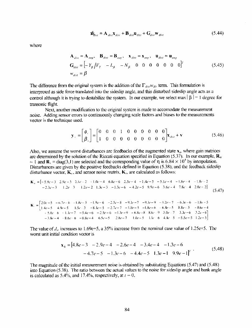
_i_, = A <h_,Xd,,,+ B_,Udi,, + G,_i,,w<m, (5.44)
where
A,Im : A.,g, Bdist = B ... x_i_ , = x.,,_., u m , : u<,,,,._.
c,,,,:[-Y,/v, -L, -N/_ 0 0 0 0 0 0 0]'
14'dis t = [_
(5.45)
The difference from the original system is the addition of the F<_,,,wai<term. This formulation is
interpreted as side force translated into the sideslip angle, and this disturbed sideslip angle acts as a
control although it is trying to destabilize the system. In our example, we select max 113 I= 1 degree for
transonic flight.
Next, another modification to the original system is made to accomodate the measurement
noise. Adding sensor errors to continuously changing scale factors and biases to the measurementsvector is the technique used.
[0,00,0000001y = = Xdi_ + V' , 0 0 0 0 0 0 0 0 0
(5.46)
Also, we assume the worst disturbances are feedbacks of the augmented state xa, where gain matrices
are determined by the solution of the Riccati equation specified in Equation (5.37). In our example, R,,= 1 and R, = diag(3,1 ) are selected and the corresponding value ofq is 6.84 × 10⁴ by interpolation.
Disturbances are given by the positive feedbacks defined in Equation (5.38); and the feedback sideslipdisturbance vector, K,,, and sensor noise matrix, K,,, are calculated as follows:
K. =[-5.9e-3 2.9e-3 2.1e-2 -I.0e-4 6.8e-6 2.5e-4 -1.4e-5 -5.1e-4 -1.8e-4 -1.8e-2
-2.3e-3 1.2e-3 -1.2e-2 1.3e-3 -1.3e-6 -4.2e-5 9.9e-6 3.6e-4 7.8e-4 2.0e-2](5.47)
=[2.0e-5 -6.7e-6 -I.8e-5 -I.9e-6 -2.5e-8 -9.1e-7 -9.1e-9 -3.2e-7 -6.3e-6 -1.8e-5K / 1.4e-5 4.9e-5 1.5e-3 -8.1e-5 -2.7e-7 -l.0e-5 -I.8e-6 -6.8e-5 8.8e-5 -8.6e-4
-5.0e-6 -1.1e-7 -5.4e-6 -2.5e-6 -1.3e-9 -6.8e-8 8.6e-9 3.0e-7 3.3e-6 3.2e-6 t
-3.&_-4 -8.6e-6 -8.8e-4 6.5e-5 2.8e-7 1.0e-5 1.1e-6 4.1e-5 -5.5e-5 1.2e-3.]
The value of./,, increases to 1.69e+5, a 35% increase from the nominal case value of 1.25e+5. The
worst unit initial condition vector is
x 0 =[4.8e-3 -2.9e-4 -2.6e-4 -3.4e-4 -1.3e-6
-4.7e-5 -1.3e-6 -4.4e-5 1.3e-1 9.9e-1] r "(5.48)
The magnitude of the initial measurement noise is obtained by substituting Equations (5.47) and (5.48)into Equation (5.38). The ratio between the actual values to the noise for sideslip angle and bank angle
is calculated as 5.4%, and 17.4%, respectively, at t = 0.
84
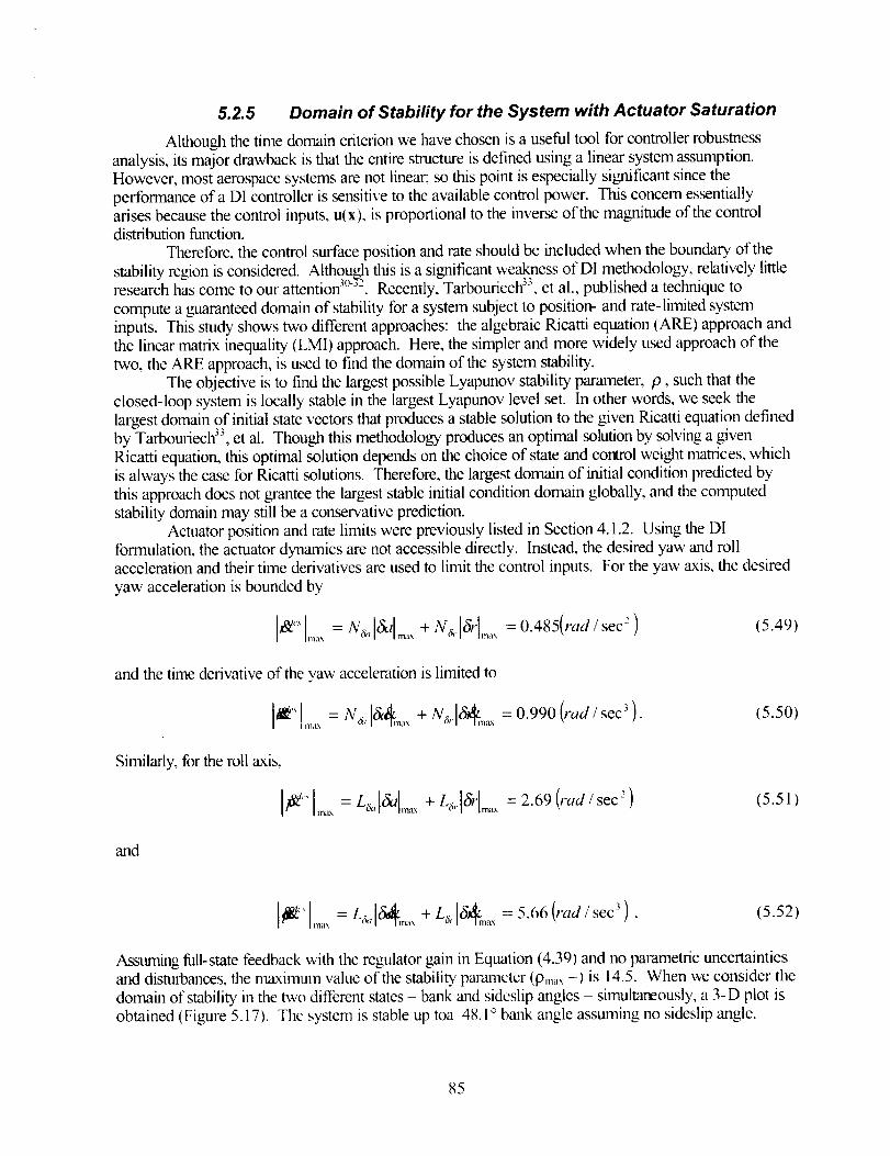
5.2.5 Domain of Stabifity for the System with Actuator Saturation
Although the time domain criterion we have chosen is a useful tool for controller robustnessanalysis, its major drawback is that the entire structure is defined using a linear system assumption.
However, most aerospace systems are not linear; so this point is especially significant since the
performance of a DI controller is sensitive to the available control power. This concern essentiallyarises because the control inputs, u(x), is proportional to the inverse of the magnitude of the controldistribution function.
Therefore, the control surface position and rate should be included when the boundary of the
stability region is considered. Although this is a significant weakness of DI methodology, relatively littleresearch has come to our attention 3_"-"_.Recently, Tarbouriech 33, et al., published a technique to
compute a guaranteed domain of stability for a system subject to position- and rate-limited system
inputs. This study shows two different approaches: the algebraic Ricatti equation (ARE) approach andthe linear matrix inequality (LMI) approach. Here, the simpler and more widely used approach of the
two, the ARE approach, is used to find the domain of the system stability.
The objective is to find the largest possible Lyapunov stability parameter, p, such that theclosed-loop system is locally stable in the largest Lyapunov level set. In other words, we seek the
largest domain of initial state vectors that produces a stable solution to the given Ricatti equation defined
by Tarbouriech 33, et al. Though this methodology produces an optimal solution by solving a Nven
Ricatti equation, this optimal solution depends on the choice of state and com'ol weight matrices, which
is always the case for Ricatti solutions. Therefore, the largest domain of initial condition predicted bythis approach does not gralatee the largest stable initial condition domain globally, and the computed
stability domain may still be a conservative prediction.Actuator position and rate limits were previously listed in Section 4.1.2. Using the DI
formulation, the actuator dynamics are not accessible directly. Instead, the desired yaw and rollacceleration and their time derivatives are used to limit the control inputs. For the yaw axis, the desired
yaw acceleration is bounded by
/_'" ,...... = Na,, &' ma, + Na,. &J ..... = 0.485(rad/sec e ) (5.49)
and the time derivative of the yaw acceleration is limited to
= + Na, =0.990(rad/sec- ). (5.50)
Similarly, for the roll axis,
J/_"' ,,,,_, = La,' 6aJm,_.,+ La, j& ,,_,_ = 2.69 (tad/sec _) (5.51 )
and
_' J,,,,,,= La'J6_",,_ + La' 6_ m_' = 5.66 (,'ad/sec3) . (5.52)
Assuming full-state feedback with the regulator gain in Equation (4.39) and no parametric uncertaintiesand disturbances, the maximum value of the stability parameter (9ma_ =) is 14.5. When we consider the
domain of stability in the two different states- bank and sideslip angles- simultareously, a 3-D plot is
obtained (Figure 5.17). The system is stable up toa 48.1 ° bank angle assuming no sideslip angle.
85

Similarly, the system is stable up to 1.59 ° sideslip assuming no bank angle. The system is not
guaranteed to be stable outside of this domain.
60 ......
50
40
o 30
20
14_?
02
!.59 1.5
1
Sideslip Angle (de9) 0 010
3020
Bank Angle (deg)
Figure 5.17 Stability boundary
5O
5.2.6 Change in Domain of Stability due to Control SurfaceActuator Failure
This nonlinear analysis next examines the stability domain in the event of a control surfaceactuator failure. This process changes the limits on the position and rates of the input vectors. Six
failure modes are considerd, and results are compared to the nominal case where no control surfaceactuator failure has taken place. The nominal and failure mode cases that are considered are the: ( 1)
nominal case, (2) one aileron failure case, (3) one rudder failure case, (4) one aileron and one rudderfailure case, (5) two aileron actuators failure case, and (6) two rudder actuators failure case. Also, as in
the previous section, perturbations on the inital conditions are limited to bank and sideslip angles. Figure
5.18 summarizes the results and their associated cross-sectional top view. This figure clearly illustrates
the difference in stability Lyapunov levels due to different constraints on control inputs. As predicted,
the nominal case, where none of the control surface actuators are failed (and the largest amount of
control power is available), shows the highest level of stability. The ratio, compared to the nominalstability domain, for all six cases is summarized in Figure 5.19.
86

00
Figu re 5.18
", IIIIIr ! ! l [ l ! [ l I
5 10 15 20 25 30 35 40 45 50
Bank Angle (deg)
Change in domain ofstabitio, duet_ .... ,..t ._,"'_....... ,.,,-,,_,. •-r.]'allure
Case I [ X-38 V-201 /@M= 1.05 ]
100 ]
9O
8O
70
O
_. 6o
_ 5o
20
10
m _
m _m
- Case4 --
_ Trim Poin!
X-38 V-201
@ M = 1.05
1 2 3 4 5Case Number
Figure 5.19 Area of stabifi O, comparison due to actuatorJ'ailure
87

6 Theoretical Foundations
6.1 Basic Forms of Dynamic Inversion
Dang Vu asserts that the essentials of the DI approach are most easily understood in terms of an
SISO system. Since we followed that approach in our leaming process, as described in Section 3, wehave postulated a class of linear systems affine' in control that is represented by the followingmathematical form:
,&=-f(x)+g(x)u (6.1)
y=h(x) (6.2)
where.fix) and g(x) are smooth vector fields on R" and h(x) is a smooth mapping function that maps R"into R. This system is feedback linearizable of relative degree r if state and input transformations exist.
z=_(x) z_R r
y=o_(x)+_(x)v veR
where ]3(x) _: 0 and _(x) is a diffeomorphism 'i that U'ansforms Equation (6.1) into a controllable linear
system.
Az + Bv
Following Dang Vu's rather succinct development (with some clarifications), we differentiate the
nonlinear output equation (Equation (6.2)) with respect to time and obtain
ah- ax
If the coefficient of u is zero, we continue with successive differentiations in the same fashion until a
nonzero process coefficient surfaces. Dang Vu's succinct notation, which uses the Lie derivative from
differential geometry for these repeated differentiations, is useful.
i"Affine in control" means that all transformations of finite system parameters remain finite under thecontroller's action.
_A diffeomorphism is said to occur when the scalar components of a mapping (or translbrmation) F are rtimes differentiable with r > 1 with respect to the scalar components of x (with a discrete time mapping x_
= F Xk+l ). The mapping must also be invertible; that is, Xk÷l = F "lXk÷l must hold. Invertibility implies thatF-1 exists. The scalar components of the inverse must likewise be r times differentiable. 34
88

Lt(x):_hf(x) (6.3)cX
Equation (6.3) is the Lie derivative of the scalar function h with respect to the vector field£ Higher-order derivatives have a similar form.
Using this Lie derivative notation, the output equation can be rewritten as
_h'_z=-ax_._x[f(x_h )+ g (x)u]:l._fh(x)+Lgh(x)u . (6.5)
If the second derivative in Equation (6.5) is 0 - that is, L9 h (x) = 0 - a second differentiation yields
h(x)+LgLfh(x)u. (6.6t
The differentiations end when L9 L_-lh( x ) = 0 for k = 1..... r - 1, but Lg Lrf-1 h ( x ) _: O. The last
derivative of the sequence for the output response is then
y (rl = L_ h( x ) + LgL_ -lh(x)u. (6.7)
The number r is called the relative degree of the original control equation (Equation (6.1)).If we define our coordinate transformation in terms of the Lie derivative,
z k=ek(x)=Lk-lh(x) fork= 1,2 ..... ,',
the resulting transformed set of equations is linear, of dimension r, and in a companion form called the
Brunovsky canonical form.
-0 1 0 L 0-
0 0 1 L 0
0 0 L 1 0
0 0 L 0 1
0 0 L 0 0
-0
0
z+Oi
I
v =Az+Bv (6.8)
where v = Lrfh(x) + LgLrf -lh(x )u. Vu points out that exact linearization is possible when the relative
degree t- is equal to the order of the system n and the linearized system (Equation (6.8)) is both
controllable and observable.
Since we are interested in obtaining for the linearizcd system a control law that will imposedesired behavior on the original nonlinear system, it is also necessary that we carefully examine anycontrol law in terms of stability of the nonlinear system. Obviously, that requirement suggests that we
89

transform any postulated control law back into the original coordinates.transformation as
x)
Symbolically, we can write this
with L h(x) andl3(x)- 1L#-Uh(x) LgL. -lh(x)
6.2 Stability and Robustness Analyses
In this section, stability and robustness analyses are described for the DI controller. The mostcommonly used methodology used to analyze robustness of linear systems using DI controllers is based
on the structured singular value (p) and a technique now widely described in tile literature as M-analysis.
However, p-analysis is not the only method used to examine the stability and robustness of DI-basedcontrollers.
6.2.1 Linear Fractional Transformations
LFTs are used to integrate parameter variations (uncertainty) into the system under _-analysis.
As the first step in the p-analysis procedure, all parameter variations are collected into an uncertaintymatrix in LFT form. Then, p-analysis looks for the smallest variation in these parameters that drive the
system to instability. In this section, the methodology to create an LFT form is explained.Suppose we have a linear system that is described by the following:
ax + bu
y=x(6.9)
Now, we assume that the value of a varies between a- and a+ .
a- _<a <_a + (6.10)
where
a- = Iowerlimit of variation in a
a + = upper limit of variation in a
This relation can be rewritten in terms of nominal value of a, a n°m , as
k18aa = a n°m + (6. ! 1)
1- k28 a '
where
9O

a n°m = nominal value of a
2(a+-_)(a-a -)k 1 =
a + -a--
(a+k 2 -
a+ - a-
-1<8 a <_1
When the upper and lower variations from the nominal values are equal - that is, when
a - an°m I= a- - a n°m -then the previous equation simplifies toI
where
a = a n°m + k8 a ,
an°m = nominal value of a
k = a + - a n°m =a n°m -a-
-1<8 a <1
The perturbation in a described in Equation (6.11) is integrated into Equation (6.9) and is now
expressed in state-space form by introducing the fictitious terms z a and w a as
(6.12)
= k 2
0
(6.13)
The block diagram in Figure 6.1 (above) corresponds to the state-space expression (Equation
(6.13)). Here, we have completely separated what is known, the G matrix, from what is uncertain, A.We treat A as uncertain; but, we do know its range: -1 < A < 1. For now, uncertainty in a alone is
considered. The next case to be considered is the case when there is an uncertainty in h. This case,
variation in h, is expressed similar to the previous case as
[ lak 'rx=o ,1 0 L u
(6.14)
where
91
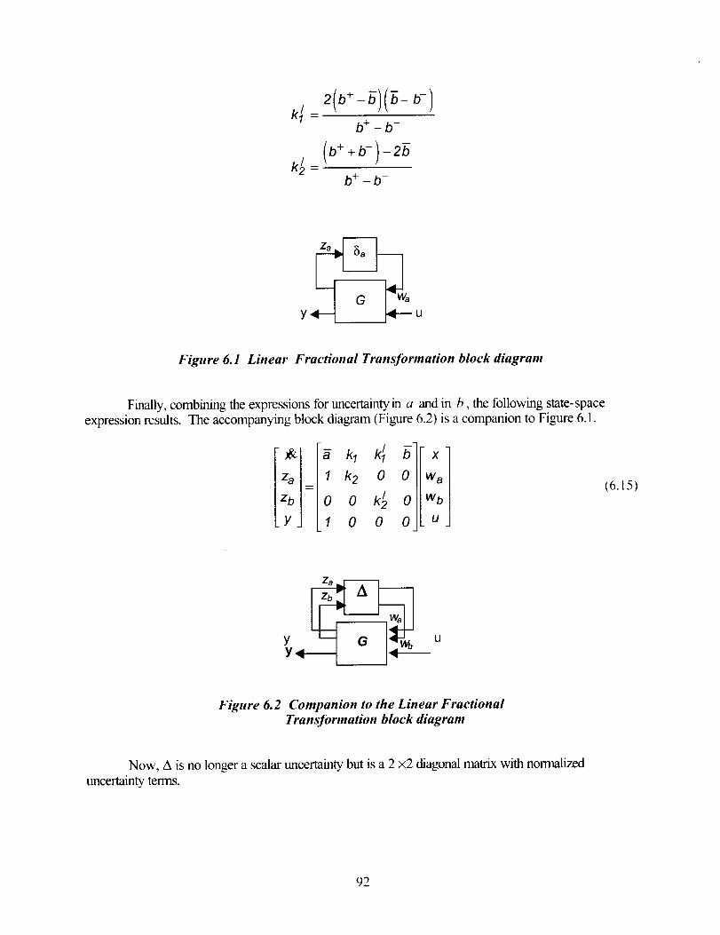
k; )b + - b-
k_,_(b++b-)-2_b+ - b-
y u
Figure 6.1 Linear Fractional Trans]brmation block diagram
Finally, combining the expressions for uncertainty in a and in b, the following state-space
expression results. The accompanying block diagu'am (Figure 6.2) is a companion to Figure 6.1.
Za =
-_ ._ ._ -51 k 2 0 0
0 0 k/2 0
1 0 0 0
Wa(6.15)
U
Figure 6.2 Companion to the Linear Fractional
Transformation block diagram
Now, A is no longer a scalar uncertainty but is a 2 x2 diagonal matrix with normalized
uncertainty terms.
92

A= 6b(6.16)
Again, we have separated what is known from what is uncertain but bounded. Since A is no longer ascalar, we have to make another choice for a norm: the maximum singular value. It is not difficult to see
that _-(A) < 1. A very important observation is that the uncertain element A has a fixed structure: adiagonal matrix consisting of the individual uncertainties in a and b. Thus, unstructured uncertainty at
the component level has become structured uncertainty at the system level. LFTs are the mathematicaltools that allow us to provide this systemic structure for the uncertainty.
6.2.2 Other Types of Uncertainty Models
Other than the parametric unce_inty described in Section 6.2.1, there are at least two other
types of uncertainty models. These are Unmodeled Dynamics or Uncertainty at the Input andUncertainty at the Output models. The major difference between parametric uncertainty and the other
two types of uncertainties is that parametric uncertainties are real-valued while the other types ofuncertainties are complex-valued perturbations. The two types of uncertainty models are explained in
the following subsections.
6.2.2.1 Unmodeled Dynamics (Uncertainty at the Input)
During the linearization process, higher-order terms in aircraft equations of motion are ignored.
Also, other uncertainties arise due to aeroelasticity, control surface variations, and vehicle flexibility.
Usually, the plant model is a good system representation term at low- to mid-fi'equency inputs, butmodeling uncertainties become larger with high-frequency inputs. Instead of attelnpting to include all
modeling uncertainties, the modeling uncertainties are treated as additives to the plant inputs. Figure 6.3
shows a general block diagram representing this approach to accounting for uncertainty at the plant
input.
Figure 6.3 Unmodeled Dynamics block diagram
p-
This type of uncertainty is parameterized with two elements, I_,,, and A,,,. _I;,, is a weightingtransfer function (assumed to be known) that reflects the amount of uncertainty in a model with respect
to frequency. The other parameter, A,,,, is a stable unknown transfer function that nevertheless satisfiesthe condition [ IA,,ll c<< 1.
6.2.2.2 Uncertainty at the Output
Similar to Unrnodeled Uncertainty, uncertainty of the measurements is modeled as Uncertaintyat the Output. A block diagrarn representing how this type of uncertainty is modeled is shown in Figure6.4.

Figure 6.4 Uncertainty at the Output block diagram
6.2.3 Structured Singular-Value Analysis (p-Analysis)
Now that we know how to represent uncertainties in the system using LFTs, we must turn our
attention to analyzing the robustness of systems modeled in this fashion. We follow the most common
practice today by basing our analysis on the structured singular value, _t, and using available softwaretools to perform the p-analysis. The technique is based on the following theorem:
Robust Stability ¢_BA_(M11(jo)))<1 V o) (6.17)
where Mz/is the left upper comer block of M; i.e.,
1M(jo)) LMzl(j(o ) M22(Jo)) J
(6.18)
and the function lttA is defined as
1
BA (M)- min{_(A): A_ A, det(I-MA): O} (6.19)
where A_:{diag(A 1, A 2 ..... An) ] .
According to this theorem, B_ is a function of M that depends on the structure of __A. pz is the
reciprocal of the smallest A (where we use 8 as the norm) we can find for the set __Athat makes the
matrix I - MA singular. If no such A exists, p6 is taken to be zero.
The general framework and the p-analysis transformation are shown in Figure 6.5.
94
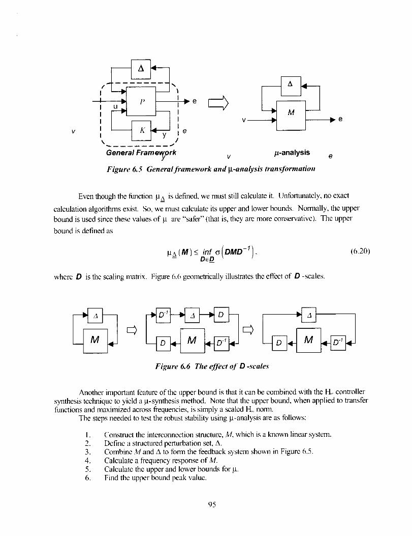
V
IIIIII
I\ /
General Fram ev_ork
Figure 6.5
v fl-analysis
Genera�framework and _t-analysis transfbrmation
e
Even though the function HA is defined, we must still calculate it. Unfortunately, no exact
calculation algorithms exist. So, we must calculate its upper and lower bounds. Normally, the upper
bound is used since these values of _t are "safer" (that is, they are more conservative). The upper
bound is defined as
o(oMo'),- D_D
(6.20)
where D is the scaling matrix. Figure 6.6 geometrically illustrates the effect of D -scales.
©
Figure 6. 6 The effbct of D -scales
Another important feature of the upper bound is that it can be combined with the I-L controller
synthesis technique to yield a p-synthesis method. Note that the upper bound, when applied to transferfunctions and maximized across frequencies, is simply a scaled 1¢,, norm.
The steps needed to test the robust stability using la-analysis are as follows:
I.
2.3.
4.
5.6.
Construct the interconnection structure, M, which is a known linear system.
Define a structured perturbation set, A.Combine M and A to form the feedback system shown in Figure 6.5.
Calculate a frequency response of M.
Calculate the upper and lower bounds for _t.
Find the upper bound peak value.
95

7. If pp_.,_< 1: pass: if P.l,e,,k> 1: fail.
96
7 Bibliography
t Krener, A. J., "On the Equivalence of Control Systems and Linearizations of Nonlinear Systems,"
SIAM Journal qf Control and Optimization, Vol. 11, 1973, pp. 670-676.
2 Brockett, R. W., "Feedback [nvariants for Nonlinear Systems," Proceedings q/ Vii IFA C Congress,
Helsinki, Finland, 1978, pp. 1115- I 120.
3 Falb, P. L. and Wolovich, W. A., "Decoupling in the Design and Synthesis of Multivariable Control
Systems," IEEE Transactions oJ'Automatic Control, AC-12, Vol. 6, 1967, pp. 651-659.
4 Singh, S. N. and Rugh, W. J., "Decoupling in a Class of Nonlinear Systems by State Variable
Feedback," Transactions o/ASME Journal qf Dymzmic Systems MeasuremeHts and Control, Vol.
94, 1972, pp. 323-329.
5 Freund, E., "Design of Time-Variable Multivariable Systems by Decoupling and by the Inverse,"
IEEE Transactions qlAutomatic Control, AC- i 6, Vol. 2, 1971, pp. 183- 185.
_'Porter, W. A., "Diagonalisation and Inverses for Nonlinear Systems," hztermltiomd Jourmtl qf
Control, Vol. 10, 1970, pp. 252-264.
: Isidori, A., Krener, A. J., Giorgi, C., and Monaco, S., "Nonlinear Decoupling Via Feedback:
a Differential Geometry Approach," 1EEE Transactions q] Automatic Control, AC-26, 1981, pp.
331-345.
Bymes, W. A., "Diagonalisation and Inverses for Nonlinear Systems," hlternational Jourmd _/"
Control, Vol. 10, 1970, pp. 252-264.
'_Bugaski, D. J., Enns, D. F., and Elgersma, M. R., "A Dynamic Inversion Based Control with
Application to the F- 18 HARV," AIAA Paper 90-3407, Proceedings q[the AIAA Guidance.
Navigation, and Control ConIerence, Portland, OR, 1990, pp. 826-839.
HJHoneywell Technolob, y Center and Houston Engineering Center, "Application q/MA CH to X-38
Drop Test Vehicle," HTC Contract Number 7028327, for NASA Johnson Space Center, June 1997.
_ Balas, G. J., Doyle, J. C., Glover, K., Packard, A., and Smith, R., _t-Analysis aml Synthesis
TOOLBOX for Use with MA TLAB, The Mathworks Inc., First Edition, July 1993.
t2 Honeywell Technology Center, Lockheed Martin Skunk Works, and Lockheed Martin Tactical
Aircraft Systems, "Application qlMultivariable Control Theoo, to Aircra/t Control La_w: Final
Report." Mtdtivariahle Con trol Design Gtddelines,'" WL- TR- 96- 3099, Flight Dynamics Directorate,
Wright Laboratory, Air Force Materiel Command, Wright-Patterson AFB, OH 45433-7562, May,
1996.
97

_3Balas,G.J.,Garrard,W.L. andReiner,J.,"RobustDynamicInversionControlLawsfor AircraftControl,"AIAA Paper92-4329,Proceedings of the AIAA Guidance, Navigation and Control
Conference, Hilton Head Island, SC, Aug. 1992, pp. 192-205.
14Anon., "Militarap Standard Flying Qualities of Piloted Aircraft," MiI-STD- 1797A, Jan. 30, 1990.
_5Enns, D., Bugajski, D., Hendrick, R. and Stein, G., "Dynamic Inversion: An Evolving Methodology
for Flight Control Design," International Journal of Control, Vol. 59, No. 1, 1994, pp. 71-91.
_6NASA Johnson Space Center, "Shuttle Engineering Simulator," July 1993.
_7Snell, S.A. and Stout, P.W., "Robust Control of Angle of Attack Using Dynamic Inversion Combined
with Quantitative Feedback Theory," AIAA Paper 96-3783, Proceedings _ffthe AIAA Guidance,
Navigation and Control Cmference, Hilton Head Island, SC, July 1996, pp. t-12.
_sBrinker, J.S. and Wise, K.A., "Stability and Flying Qualities Robustness of a Dynamic Inversion
Aircraft Control Law," Journal of Guidance, Control, and Dynamics, Vol. 19, No. 6, Nov.-Dec.,
1996, pp. 1270- 1277.
J_Suikat, R., Donaldson, K. and Downing, D., "Analysis of a Candidate Control Algorithm for a Ride-
Quality Augmentation System," Journal of Guidance, Control, and Dynamics, Vol. 12, No. 4, July-
Aug. 1989, pp. 505-513.
__oIto, D. and Valasek, J., "Robust Dynamic Inversion Controller Design and Analysis to the
X-38 Vehicle," AIAA Paper 2001-4380, AIAA Guidance, Navigation and Control Cot1[brence,
Montreal, Canada, Aug. 2001.
2_Doyle, J. C. and Stein, G., "Multivariable Feedback Design: Concepts for a Classical/
Modem Synthesis,'" Proceedings of lEEE Transactions on Automatic Control, Vol. AC-26, No. I,
February 1981, pp. 4-16.
22Lin, J. M., Chang, C. H. and Tsai, H. L., "Optimal Feedforward and Feedback Controllers Designed
by LQG/LTR Method," Journal o['the Chinese Institute of Engineers, Vol. 20, No. 1, 1997, pp.
57-66.
23Ridgely, D. B., Banda, S. S., McQuade, T. E. and Lynch, P. J. "Linear-Quadratic-Gaussian
with Loop-Transfer-Recovery Methodology for an Unmanned Aircraft," Journal of Guidance,
Control, and Dynamics, Vol. 10, Jan.-Feb. 1987, pp. 82-89.
24Maciejowski, J. M., Multivariable Feedback Design, Addison-Wesley Publislfing Company, 1992.
25Athans, M., "Tutorial on the LQG/LTR Method," MAA Paper 97-3607, 1997, pp. 755-769.
26Anon., "X-38 VI31R FCS Requirements," NASA Johnson Space Center Internal Memo, May
2000.
27Stevens, B. L. and Lewis, F. L., Aircrq/t Control and Simulation, John Wiley & Sons, Inc., New
York, 1992.
98


I Form ApprovedREPORT DOCUMENTATION PAGE II OMB No. 0704-0188
Public reporting burden for this collection of information is estimated to average 1 hour per response, inOuding the time for reviewing instructions, searching existing data sources, gathenng and maintaining the data
needed, and completing and reviewing the collection Of ink)rmatiorl Send comments regarding this burden estimate _r any _ther aspect _f this co_ecti_n _ inf_rmat_n' inc_uding suggesti_ns f_r reduc_ng this burden_to Washington Headquarters Services, Directorate for information Operations and Reports, 1215 Jefferson Davis Highway, Surte 1204, Arlington, VA 22202-4302, and to the Office of Management and Budget,Pacerwork Reduction Proect {0704-0188_. Washinaton. DC 205(33
1 A_FNC:.Y 11RF C)NI Y (I _v_.. Rl_nk) ) RI=PORT I-)A-I'F .3 RFPC)RT TYPI:= ANR I")A"r_R C:C)VI=RFI-)
March 2002 NASA Technical Paper
F_ FI INDINQ NI IMP, OR.C:;4 TITI F ANt) RI IRTITI F
Reentry Flight Vehicle Controls Design Guidelines: Dynamic Inversion
6. AUTHOR(S)
Daigoro Ito,* Jennifer Georgie,** John Valasek,** Donald T. Ward*
7. PERFORMING ORGANIZATION NAME(S) AND ADDRESS(ES)
Lyndon B. Johnson Space Center
Houston, Texas 77058
9. SPONSORING/MONITORING AGENCY NAME(S) AND ADDRESS(ES)
National Aeronautics and Space Administration
Washington, DC 20546-0001
8. PERFORMING ORGANIZATION REPORTNI IMP.FR£
S-881
10. SPONSORING/MONITORING"/'_l=klc'tY #I='I:_'_.PT kll IIL.IRI:::I_
T P-2002-210771
1 1 RI IPPI FMFNTARY Nc)'rFR
*Lyndon B. Johnson Space Center, Houston, Texas
**Flight Simulation Laboratory, Texas Engineering Experiment Station, Texas A&M University, College Station, Texas
12a. DISTRIBUTION/AVAILABILITY STATEMENT
Available from the NASA Center for AeroSpace Information (CASI)7121 Standard
Hanover, MD 21076-1320 Subject Category: 3(.)
12b. DISTRIBUTION CODE
1:3 ARRTRA_T (M_irnttrn )DO wnrd._}
This report addresses issues in developing a flight control design for vehicles operating across a broad flight regime and with highly
nonlinear physical descriptions of motion. Specifically it addresses the need for reentry vehicles that could operate through reentry
from space to controlled touchdown on Earth. The latter part of controlled descent is achieved by parachute or paraglider - or by an
automatic or a human-controlled landing similar to that of the Orbiter. Since this report addresses the specific needs of human-carrying
(not necessarily piloted) reentry vehicles, i1 deals with highly nonlinear equations of motion, and their generated control systems must
be robust across a very wide range of physics. Thus, this report deals almost exclusively with some form of dynamic inversion (DI).
Two vital aspects of control theory - noninteracting control laws and the transformation of nonlinear systems into equivalent linear
systems - are embodied in DI. Though there is no doubt that the mathematical tools and underlying theory are widely available, there
are open issues as to the practicality of using DI as the only or primary design approach for reentry _,ehicles. This report provides a set
of guidelines that can be used to determine the practical usefulness of the technique.
14. SUBJECT TERMS
flight control: spacecraft control: reentry vehicles: dynamics: equations of motion:
nonlinear equations: control systems design
17. SECURITY CLASSIFICATION 18 SECURITY CLASSIFICATION
Unclassified Unclassified
Standard Form 298 (Rev Feb 89) (MS Word Mar 97)
Prescribed by ANSI Std. 239-18
298-102
15. NUMBER OF
116
16. PRICE CODE
19. SECURITY CLASSIFICATION
Unlimited
20. LIMITATION OF ABSTRACT
Unlimited
NSN 7540-01-280-5500

2_Dang Vu, B., "Nonlinear Dynamic Inversion Control," Lecture Notes in Control and hl['ormation
Sciences 224." Robust Flight Control: A Design Challenge, Springer, London, 1997, p. 111.
29Ghaoui, L. E., Carrier, A. and Bryson, A. E. "Linear Quadratic Minimax Controllers," Journal oj"
Guidance, Control. and Dynamics, Vol. 15, No. 4, July-Aug. 1992, pp. 953-961.
3oHess, R. A. and Snell, S. A. "Flight Control System Design with Rate Saturating Actuators," Journal
qjGuidance, Control, and Dynamics, Vol. 20, No. 1, Jan.-Feb. 1997, pp. 90-96.
31Snell, S. A. and Hess, R. A. "Robust, Decoupled, Flight Control Design with Rate-Saturating
Actuators," Journal q[Guitkmce, Control, and Dynamics, Vol. 21, No. 3, May-June 1998, pp.
361-367.
32Snell, S. A. "Decoupling Control Design with Applications to Flight," Journal of Guidance, Control,
and Dynamics, Vol. 21, No. 4, July-Aug. 1998, pp. 647-655.
33Tarbouriech, S., Garcia, G., and Henrion, D., "Local Stabilization of Linear Systems with Position
and Rate Bounded Actuators," Proceedings q[ 14th Triennial World Congress, Be_jing, P.R. China,
F-2e-02-5, 1999, pp. 459-464.
34Nayfeh, A. H. and Balachandran, B., Applied Nonlinear Dynamics, John Wiley & Sons, Inc., New
York, 1995, pp. 2-4.
99