Embed Size (px)
Citation preview

Greenhouse gas emission
reductions enabled by products
from the chemical industry
ECOFYS Netherlands B.V. | Kanaalweg 15G | 3526 KL Utrecht| T +31 (0)30 662-3300 | F +31 (0)30 662-3301 | E [email protected] | I www.ecofys.com
Chamber of Commerce 30161191
Greenhouse gas emission reductions enabled
by products from the chemical industry
By: Edgar van de Brug, Annemarie Kerkhof, Maarten Neelis and Wouter Terlouw
Date: 10 March 2017
© Ecofys 2017 by order of the International Council of Chemical Associations
ECOFYS Netherlands B.V. | Kanaalweg 15G | 3526 KL Utrecht| T +31 (0)30 662-3300 | F +31 (0)30 662-3301 | E [email protected] | I www.ecofys.com
Chamber of Commerce 30161191
Foreword
The chemical industry plays an essential role in enabling other industries to improve their energy
efficiency and reduce their greenhouse gas emissions (GHG). This is achieved by using chemical
products and technologies. Several ICCA reports have underpinned the scale of the chemical industry’s
contribution to enabling emissions reduction, also known as “avoided emissions”. “Innovation for
Greenhouse Gas Reductions: A life cycle quantification of carbon abatement solutions enabled by the
chemical industry” (2009) and “ICCA Building Technology Roadmap: The Chemical Industry’s
Contribution to Energy and Greenhouse Gas Savings in Residential and Commercial Construction”
(2013) are the most relevant examples.
Subsequently, to improve consistency in the assessment and reporting of avoided emissions, ICCA and
WBCSD published a practical guidance document entitled “Addressing the Avoided Emissions
Challenge” (2013).
Building on the past work, ICCA conducted a new study on the maximum potential for annual GHG
emissions reduction enabled by the chemical industry for selected six solutions in a specific year.
Moreover, a scenario analysis on annual GHG emissions reduction enabled by the chemical industry for
selected six solutions in 2030 is being prepared.
The objective of this study is to assess the global contribution of the chemical industry to selected six
solutions in the context of limiting average temperature rise to 2 degrees Celsius, as agreed on in the
Paris Agreement in 2015. Despite the small number of solutions considered, the magnitude of chemical
products’ contribution is remarkable. The study on the maximum potential indicates that even a higher
reduction seems feasible in 2030 with appropriate and enabling policies in place.
Bunro Shiozawa
Associate Officer, Sumitomo Chemical Corporation and
Chairman, ICCA Energy and Climate Change Leadership Group

ECOFYS Netherlands B.V. | Kanaalweg 15G | 3526 KL Utrecht| T +31 (0)30 662-3300 | F +31 (0)30 662-3301 | E [email protected] | I www.ecofys.com
Chamber of Commerce 30161191
Acknowledgements
This publication was prepared by the Ecofys team of experts managed by Edgar van de Brug and
Maarten Neelis and further consisting of Wouter Terlouw and Annemarie Kerkhof. The Ecofys team
developed the global stock-based analysis, including a decomposition methodology for attributing
reductions to factors in scenario analysis.
This study would have been impossible without a strong support from the ICCA Energy and Climate
Change Leadership Group members under the Supervision of Kiyoshi Matsuda (Mitsubishi Chemical
Holdings) and William Garcia (Cefic). The ICCA members who contributed with their technical expertise
and invaluable insights into the analysis are BASF (Andreas Horn and Nicola Paczkowski), Braskem
(Yuki Kabe), ExxonMobil (Baudouin Kelecom, Abdelhadi Sahnoune and Marvin Hill), Shell ( Bob Cooper)
and Solvay (Pierre Coërs).
This study benefited from input provided from experts in CIRAIG who assessed and provided comments
to an advanced draft of the study.
ECOFYS Netherlands B.V. | Kanaalweg 15G | 3526 KL Utrecht| T +31 (0)30 662-3300 | F +31 (0)30 662-3301 | E [email protected] | I www.ecofys.com
Chamber of Commerce 30161191
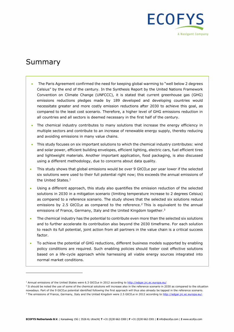
Summary
• The Paris Agreement confirmed the need for keeping global warming to “well below 2 degrees
Celsius” by the end of the century. In the Synthesis Report by the United Nations Framework
Convention on Climate Change (UNFCCC), it is stated that current greenhouse gas (GHG)
emissions reductions pledges made by 189 developed and developing countries would
necessitate greater and more costly emission reductions after 2030 to achieve this goal, as
compared to the least cost scenario. Therefore, a higher level of GHG emissions reduction in
all countries and all sectors is deemed necessary in the first half of the century.
• The chemical industry contributes to many solutions that increase the energy efficiency in
multiple sectors and contribute to an increase of renewable energy supply, thereby reducing
and avoiding emissions in many value chains.
• This study focuses on six important solutions to which the chemical industry contributes: wind
and solar power, efficient building envelopes, efficient lighting, electric cars, fuel efficient tires
and lightweight materials. Another important application, food packaging, is also discussed
using a different methodology, due to concerns about data quality.
• This study shows that global emissions would be over 9 GtCO2e per year lower if the selected
six solutions were used to their full potential right now; this exceeds the annual emissions of
the United States.1
• Using a different approach, this study also quantifies the emission reduction of the selected
solutions in 2030 in a mitigation scenario (limiting temperature increase to 2 degrees Celsius)
as compared to a reference scenario. The study shows that the selected six solutions reduce
emissions by 2.5 GtCO2e as compared to the reference.2 This is equivalent to the annual
emissions of France, Germany, Italy and the United Kingdom together.3
• The chemical industry has the potential to contribute even more than the selected six solutions
and to further accelerate its contribution also beyond the 2030 timeframe. For each solution
to reach its full potential, joint action from all partners in the value chain is a critical success
factor.
• To achieve the potential of GHG reductions, different business models supported by enabling
policy conditions are required. Such enabling policies should foster cost effective solutions
based on a life-cycle approach while harnessing all viable energy sources integrated into
normal market conditions.
1 Annual emissions of the United States were 6.3 GtCO2e in 2012 according to http://edgar.jrc.ec.europa.eu/ 2 It should be noted the use of some of the chemical solutions will increase also in the reference scenario in 2030 as compared to the situation
nowadays. Part of the 9 GtCO2e potential identified following the first approach will thus also already be tapped in the reference scenario. 3 The emissions of France, Germany, Italy and the United Kingdom were 2.5 GtCO2e in 2012 according to http://edgar.jrc.ec.europa.eu/.
ECOFYS Netherlands B.V. | Kanaalweg 15G | 3526 KL Utrecht| T +31 (0)30 662-3300 | F +31 (0)30 662-3301 | E [email protected] | I www.ecofys.com
Chamber of Commerce 30161191
Context, project goal and approach
“The International Council of Chemical Associations (ICCA) firmly supports the UN Framework
Convention on Climate Change (UNFCCC) and welcomes its successful outcome during the 21st meeting
of the Conference of the Parties (COP21). The Paris Agreement is an important framework for
international cooperative action that reflects strong political commitment by all economies to the
measurement, monitoring and reporting of nationally determined contributions to reduce greenhouse
gas (GHG) emissions.” 4
The Paris Agreement confirmed the need for higher level of GHG emissions reduction in all countries
and all sectors in the coming century. In the IPCC Climate Change 2014 Synthesis report it is stated
that “many adaptation and mitigation options can help address climate change, but no single option is
sufficient by itself. Effective implementation depends on policies and cooperation at all scales (…)”.5 The
chemical industry is part of the life cycle of many everyday products. This unique position offers the
chemical industry opportunities to reduce GHG emissions throughout all parts of society.
In this report six representative solutions have been selected and studied. The chemical industry
contributes to the value chain emission reductions these solutions enable: wind and solar power,
efficient building envelopes, efficient lighting, electric cars, fuel efficient tires and lightweight materials.
A seventh important solution, the use of packaging material to reduce food losses, is also commented
on using a different methodology, due to concerns about data quality.
These solutions improve energy efficiency or contribute to an increase of renewable energy supply. The
solutions represent an important share of the emission reductions enabled by contributions of the
chemical industry, but there are more solutions in other sectors as well. While the chemical industry
contributes extensively to these solutions, their contribution occurs alongside contributions from other
enabling parties in the value chain.
ICCA has been actively involved for years in efforts to quantify the potential for the value chain emission
reductions in a fact-based and transparent way. In terms of the method used, this report builds on these
studies including the innovations for GHG reductions study, the avoided emission guidelines, and the
case studies to showcase the application of the these guidelines.6,7,8 Two distinct approaches are used
in this study to quantify the emission reductions enabled by the chemical industry:
4 Taken from ICCA views on COP21, February 2016 5 IPCC, 2014. Climate Change 2014 Synthesis Report. Synthesis report of the IPCC Fifth Assessment Report (AR5) available at:
https://www.ipcc.ch/pdf/assessment-report/ar5/syr/AR5_SYR_FINAL_All_Topics.pdf. 6 ICCA, 2009. Innovations for Greenhouse Gas Reductions: A life cycle quantification of carbon abatement solutions enables by the chemical
industry. Available at: http://www.icca-chem.org/ICCADocs/ICCA_A4_LR.pdf. 7 ICCA, 2013. Addressing the Avoided Emissions Challenge: Guidelines from the chemical industry for accounting for and reporting greenhouse
gas (GHG) emissions avoided along the value chain based on comparative studies. Available at: http://www.icca-
chem.org/iccadocs/E%20CC%20LG%20guidance_FINAL_07-10-2013.pdf. 8 ICCA, 2016. Reduction of Greenhouse Gas Emissions via Use of Chemical Products – Case studies: Exemplifying the application of the ICCA
& WBCSD Avoided Emissions Guidelines.
ECOFYS Netherlands B.V. | Kanaalweg 15G | 3526 KL Utrecht| T +31 (0)30 662-3300 | F +31 (0)30 662-3301 | E [email protected] | I www.ecofys.com
Chamber of Commerce 30161191
1. Approach I: Estimated annual emission reductions if the solutions were used to their full
potential right now. In this approach, it is estimated how much higher emissions would be if the
solutions were not used at all (zero market share versus current market share) and how much
lower emissions would be if the solutions were used to their full potential right now (up to 100%
market share).
2. Approach II: Contribution of the solutions to the GHG emission reductions in 2030 in a
2 degrees Celsius mitigation scenario as compared to a reference scenario. In this approach,
it is estimated what the contribution of the solutions is to emission reductions in a mitigation scenario
(limiting temperature increase to 2 degrees Celsius) as compared to a reference scenario. The
scenarios are based on the IEA Energy Technology Perspectives 2015 (IEA ETP 2015) scenarios. The
reference scenario is based on the 6DS scenario and the mitigation scenario is based on the 2DS
scenario. Assumptions not specified in IEA ETP 2015 are determined by expert judgement.
The results from the different approaches are not directly comparable, but both provide insights in the
potential GHG emissions reduction enabled by the solutions to which the chemical industry contributes.9
The study also addresses the enabling conditions (business and policies related) needed to realise this
potential along the value chains.
Main results
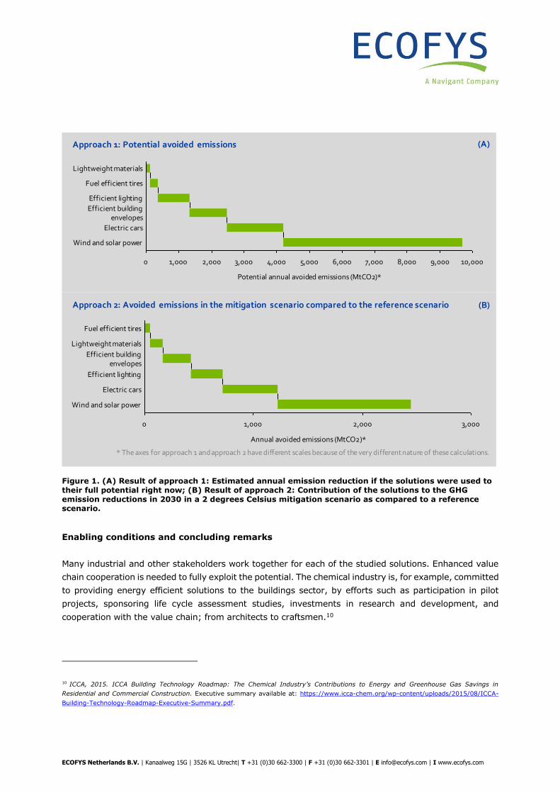
Figure 1A shows that the global annual emissions would be over 9 GtCO2e lower if the selected solutions
were used to their full potential right now. For comparison, this is substantially more than the current
annual emissions of the United States.1 Renewable energy (solar and wind power) as well as energy
efficiency measures (such as electric cars, efficient building envelopes and efficient lighting) are major
contributors to this potential.
Figure 1B shows that the selected solutions reduce emissions by 2.5 GtCO2e in 2030 in a 2 degrees
Celsius mitigation scenario as compared to a reference scenario. This is equivalent to the annual
emissions of France, Germany, Italy and the United Kingdom together.3 The relative contribution of
each of the solutions is comparable to the results obtained using the first approach.
9 The first approach investigates the potential at this moment in time, the second approach looks into the situation in 2030. Also, the use of some
of the chemical solutions will increase also in the reference scenario in 2030 as compared to the situation nowadays. Part of the potential identified
following the first approach will thus also already be tapped in the reference scenario.
ECOFYS Netherlands B.V. | Kanaalweg 15G | 3526 KL Utrecht| T +31 (0)30 662-3300 | F +31 (0)30 662-3301 | E [email protected] | I www.ecofys.com
Chamber of Commerce 30161191
Figure 1. (A) Result of approach 1: Estimated annual emission reduction if the solutions were used to their full potential right now; (B) Result of approach 2: Contribution of the solutions to the GHG emission reductions in 2030 in a 2 degrees Celsius mitigation scenario as compared to a reference scenario.
Enabling conditions and concluding remarks
Many industrial and other stakeholders work together for each of the studied solutions. Enhanced value
chain cooperation is needed to fully exploit the potential. The chemical industry is, for example, committed
to providing energy efficient solutions to the buildings sector, by efforts such as participation in pilot
projects, sponsoring life cycle assessment studies, investments in research and development, and
cooperation with the value chain; from architects to craftsmen.10
10 ICCA, 2015. ICCA Building Technology Roadmap: The Chemical Industry’s Contributions to Energy and Greenhouse Gas Savings in
Residential and Commercial Construction. Executive summary available at: https://www.icca-chem.org/wp-content/uploads/2015/08/ICCA-
Building-Technology-Roadmap-Executive-Summary.pdf.
Approach 1: Potential avoided emissions
0 1,000 2,000 3,000 4,000 5,000 6,000 7,000 8,000 9,000 10,000
Lightweight materials
Fuel efficient tires
Efficient lighting
Efficient buildingenvelopes
Electric cars
Wind and solar power
Potential annual avoided emissions (MtCO2)*
Approach 2: Avoided emissions in the mitigation scenario compared to the reference scenario
0 1,000 2,000 3,000
Efficient lighting
Fuel efficient tires
Efficient buildingenvelopes
Electric cars
Lightweight materials
Annual avoided emissions (MtCO2)*
Wind and solar power
* The axes for approach 1 and approach 2 have different scales because of the very different nature of these calculations.
(A)
(B)
ECOFYS Netherlands B.V. | Kanaalweg 15G | 3526 KL Utrecht| T +31 (0)30 662-3300 | F +31 (0)30 662-3301 | E [email protected] | I www.ecofys.com
Chamber of Commerce 30161191
An enabling policy environment is needed, stimulating greenhouse gas emission reductions along the full
value chain, including use and end-of life phases.
• Governments should establish technology neutral policies which enable cost effective renewable
energy to grow and contribute to greenhouse gas emission reductions, while ensuring the reliable,
affordable, and non-intermittent supply of electricity. Financial support should only be available for
technology development of pre-commercial innovative technologies. All technologies should be
integrated into normal market conditions, removing subsidies as soon as the technology is
commercial.
• Energy efficient measures have a large potential of saving energy and reducing greenhouse gas
emissions worldwide. Governments should, for example, set energy efficiency standards, encourage
manufacturers to provide correct and easy-to-understand information, and take necessary actions to
raise public awareness depending on regional/national circumstances.
Further work is needed, also by the modelling teams, to shed more light on the exact impact mitigation
will have on the material demand and resulting emissions of the chemical industry itself; a somewhat
unexplored issue in the current modelling due to the focus on the use phase of emissions in the scenario
work.
The selected solutions highlight the opportunities of the chemical industry in a low carbon world. The
chemical industry has the potential to contribute even more and to further accelerate its contribution also
beyond the 2030 timeframe. For all solutions to be used widely, joint action from all partners in the value
chain is needed, as well as different business models, supported by sufficiently enabling policy conditions
at an adequate level.
ECOFYS Netherlands B.V. | Kanaalweg 15G | 3526 KL Utrecht| T +31 (0)30 662-3300 | F +31 (0)30 662-3301 | E [email protected] | I www.ecofys.com
Chamber of Commerce 30161191
Table of contents
Introduction 1
Approach 4
2.1 Methodological background 4
2.2 Methodological approach 7
Results 12
3.1 Current avoided emissions potential (Approach 1) 12
3.2 Contribution in 2030 in a mitigation scenario (Approach 2) 13
Wind and solar power 14
Efficient building envelopes 16
Efficient lighting 18
Fuel efficient tires, lightweight materials and electric cars 20
Conclusion 22
Appendix 24
5.1 Emission factors 24
5.2 Wind and solar power 26
5.3 Efficient building envelopes 33
5.4 Efficient lighting 46
5.5 Transport: Fuel efficient tires 57
5.6 Transport: Lightweight materials for cars 62
5.7 Transport: Electric cars 70
5.8 Transport: Scenario analysis 76
5.9 Packaging 79
5.10 Decomposition analysis 81
1
Introduction
The Paris Agreement confirmed the need for keeping global warming to “well below 2 degrees Celsius”
by the end of the century. In the Synthesis Report by the United Nations Framework Convention on
Climate Change (UNFCCC), it is stated that current greenhouse gas (GHG) emissions reductions pledges
made by 189 developed and developing countries would necessitate greater and more costly emission
reductions after 2030 to achieve this goal, as compared to the least cost scenario. Therefore, a higher
level of GHG emissions reduction in all countries and all sectors is deemed necessary in the first half of
the century. In the “Climate Change 2014 Synthesis Report” it is stated that “many adaptation and
mitigation options can help address climate change, but no single option is sufficient by itself. Effective
implementation depends on policies and cooperation at all scales (…)”.11
The International Council of Chemical Associations (ICCA) firmly supports the UNFCCC. It welcomes
the Paris Agreement as an important framework for international cooperative action that reflects strong
political commitment by all economies to the measurement, monitoring and reporting of nationally
determined contributions to reduce GHG emissions.
The chemical industry is a significant emitter of GHG emissions and is committed to reduce these
emissions via a wide range of mitigation activities. At the same time, many innovative chemical industry
products enable GHG emission reductions downstream in the value chain, also referred to as avoided
emissions, e.g. lightweight materials in cars to save fuels and insulation materials to save energy for
heating buildings. In this way, the chemical industry contributes to GHG emission reductions throughout
society and enables a low carbon world.12
Reliable and credible figures on GHG emission reductions enabled by solutions with chemical products
are essential to demonstrate the potential contribution of the chemical industry to future emission
reductions and to provide context for the development of the chemical industry’s own emissions under
a mitigation scenario. ICCA has been actively involved for years in efforts to quantify this potential in
a fact-based and transparent way.
This report builds on the previous work done by ICCA. In 2009, the study “Innovations for Greenhouse
Gas Reductions: A life cycle quantification of carbon abatement solutions enabled by the chemical
industry” was published, providing comparisons between numerous chemical products with their next
11 IPCC, 2014. Climate Change 2014 Synthesis Report. Synthesis report of the IPCC Fifth Assessment Report (AR5) available at:
https://www.ipcc.ch/pdf/assessment-report/ar5/syr/AR5_SYR_FINAL_All_Topics.pdf. 12 With the term “low carbon world”, we mean a world economy that functions well without excessive emissions of greenhouse gases like
carbon dioxide (CO2), methane (CH4), nitrous oxide (N2O), and F-gases (hydrofluorocarbons (HFCs), perfluorocarbons (PFCs), sulphur
hexafluoride (SF6) and nitrogen trifluoride (NF3)).
2
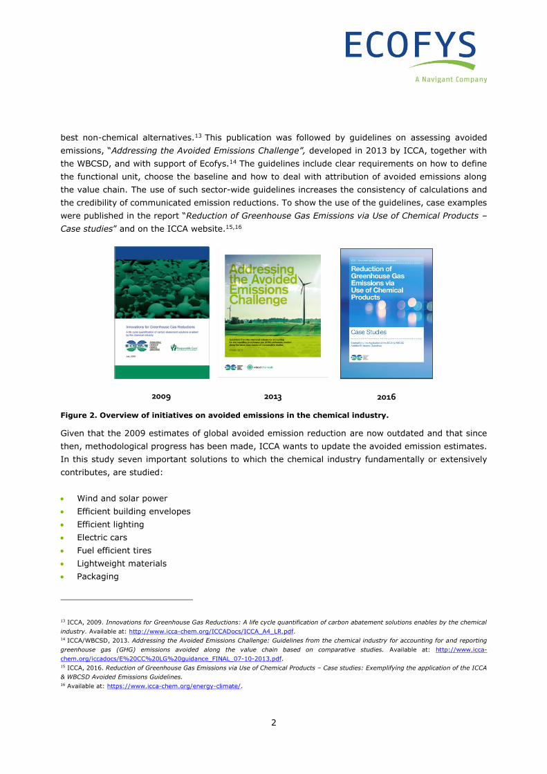
best non-chemical alternatives.13 This publication was followed by guidelines on assessing avoided
emissions, “Addressing the Avoided Emissions Challenge”, developed in 2013 by ICCA, together with
the WBCSD, and with support of Ecofys.14 The guidelines include clear requirements on how to define
the functional unit, choose the baseline and how to deal with attribution of avoided emissions along
the value chain. The use of such sector-wide guidelines increases the consistency of calculations and
the credibility of communicated emission reductions. To show the use of the guidelines, case examples
were published in the report “Reduction of Greenhouse Gas Emissions via Use of Chemical Products –
Case studies” and on the ICCA website.15,16
Figure 2. Overview of initiatives on avoided emissions in the chemical industry.
Given that the 2009 estimates of global avoided emission reduction are now outdated and that since
then, methodological progress has been made, ICCA wants to update the avoided emission estimates.
In this study seven important solutions to which the chemical industry fundamentally or extensively
contributes, are studied:
• Wind and solar power
• Efficient building envelopes
• Efficient lighting
• Electric cars
• Fuel efficient tires
• Lightweight materials
• Packaging
13 ICCA, 2009. Innovations for Greenhouse Gas Reductions: A life cycle quantification of carbon abatement solutions enables by the chemical
industry. Available at: http://www.icca-chem.org/ICCADocs/ICCA_A4_LR.pdf. 14 ICCA/WBCSD, 2013. Addressing the Avoided Emissions Challenge: Guidelines from the chemical industry for accounting for and reporting
greenhouse gas (GHG) emissions avoided along the value chain based on comparative studies. Available at: http://www.icca-
chem.org/iccadocs/E%20CC%20LG%20guidance_FINAL_07-10-2013.pdf. 15 ICCA, 2016. Reduction of Greenhouse Gas Emissions via Use of Chemical Products – Case studies: Exemplifying the application of the ICCA
& WBCSD Avoided Emissions Guidelines. 16 Available at: https://www.icca-chem.org/energy-climate/.
2009 2013 2016
3
The selected solutions help to improve energy efficiency or to contribute to an increase of renewable
energy supply. The solutions represent the lion share of the emission reductions enabled by
contributions of the chemical industry, but there are more solutions in other sectors as well.13 While
the chemical industry contributes extensively to these solutions, their contribution occurs alongside
contributions from other enabling parties in the value chain.
To illustrate the contribution of the chemical industry in enabling avoided emissions, two distinct
approaches are used:
1. Approach I: Estimated annual emission reductions if the solutions were used to their full
potential right now. In this approach, it is estimated how much higher emissions would be if the
solutions were not used at all (zero market share versus current market share) and how much
lower emissions would be if the solutions were used to their full potential right now (up to 100%
market share).
2. Approach II: Contribution of the solutions to the GHG emission reductions in 2030 in a 2
degrees Celsius mitigation scenario as compared to a reference scenario. In this approach,
it is estimated what the contribution of the solutions is in to emission reductions in a mitigation
scenario (limiting temperature increase to 2 degrees Celsius) as compared to a reference scenario.
The scenarios are based on the IEA Energy Technology Perspectives 2015 (IEA ETP 2015) scenarios.
The reference scenario is based on the 6DS scenario and the mitigation scenario is based on the 2DS
scenario. Assumptions not specified in IEA ETP 2015 are determined by expert judgement.
Finally, this report addresses the enabling conditions that are needed to realise this potential in practice.
This information can help stakeholders, like chemical industry value chain partners and national policy-
makers worldwide, to take measures to reduce GHG emissions and therefore contribute to achieving the
ambitions agreed upon at the COP21 in Paris and the related Nationally Determined Contributions (NDCs).
4
Approach
2.1 Methodological background
The goal of this study is to obtain fact-based figures on avoided emissions to demonstrate the enabling
potential of the chemical industry to de-carbonize the economy. This study builds upon the
methodological guidance provided in the “Addressing the avoided emissions challenge” guidelines.14
The use of such sector-wide guidelines increases the consistency of calculations and the credibility of
communicated emission reductions. Six principles are key in calculating of and reporting on avoided
emissions: relevance, completeness, consistency, transparency, accuracy and feasibility.
This study highlights chemical solutions that can enable emission reduction compared to conventional
solutions currently being used. The calculation of the emission reduction throughout the value chain
comes with various methodological issues, including the scope definition, the level in the value chain,
the choice of the baseline, consideration of future changes, and the attribution of avoided emissions to
different actors in the value chain.
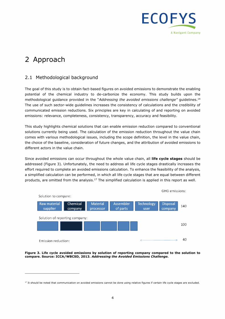
Since avoided emissions can occur throughout the whole value chain, all life cycle stages should be
addressed (Figure 3). Unfortunately, the need to address all life cycle stages drastically increases the
effort required to complete an avoided emissions calculation. To enhance the feasibility of the analysis,
a simplified calculation can be performed, in which all life cycle stages that are equal between different
products, are omitted from the analysis.17 The simplified calculation is applied in this report as well.
Figure 3. Life cycle avoided emissions by solution of reporting company compared to the solution to compare. Source: ICCA/WBCSD, 2013. Addressing the Avoided Emissions Challenge.
17 It should be noted that communication on avoided emissions cannot be done using relative figures if certain life cycle stages are excluded.
5
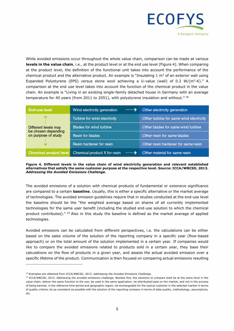
While avoided emissions occur throughout the whole value chain, comparison can be made at various
levels in the value chain, i.e., at the product level or at the end use level (Figure 4). When comparing
at the product level, the definition of the functional unit takes into account the performance of the
chemical product and the alternative product. An example is “Insulating 1 m2 of an exterior wall using
Expanded Polystyrene (EPS) versus stone wool achieving a U-value (wall) of 0.2 W/(m2∙K).” A
comparison at the end use level takes into account the function of the chemical product in the value
chain. An example is “Living in an existing single-family detached house in Germany with an average
temperature for 40 years (from 2011 to 2051), with polystyrene insulation and without.” 18
Figure 4. Different levels in the value chain of wind electricity generation and relevant established alternatives that satisfy the same customer purpose at the respective level. Source: ICCA/WBCSD, 2013. Addressing the Avoided Emissions Challenge.
The avoided emissions of a solution with chemical products of fundamental or extensive significance
are compared to a certain baseline. Usually, this is either a specific alternative or the market average
of technologies. The avoided emission guidelines require that in studies conducted at the end-use level
the baseline should be the “the weighted average based on shares of all currently implemented
technologies for the same user benefit (including the studied end-use solution to which the chemical
product contributes).” 19 Also in this study the baseline is defined as the market average of applied
technologies.
Avoided emissions can be calculated from different perspectives, i.e. the calculations can be either
based on the sales volume of the solution of the reporting company in a specific year (flow-based
approach) or on the total amount of the solution implemented in a certain year. If companies would
like to compare the avoided emissions related to products sold in a certain year, they base their
calculations on the flow of products in a given year, and assess the actual avoided emission over a
specific lifetime of the product. Communication is then focused on comparing actual emissions resulting
18 Examples are obtained from ICCA/WBCSD, 2013. Addressing the Avoided Emissions Challenge. 19 ICCA/WBCSD, 2013. Addressing the avoided emissions challenge. Besides this, the solutions to compare shall be at the same level in the
value chain; deliver the same function to the use; be used in the same application; be distributed/used on the market, and not in the process
of being banned, in the reference time period and geographic region; be exchangeable for the typical customer in the selected market in terms
of quality criteria; be as consistent as possible with the solution of the reporting company in terms of data quality, methodology, assumptions,
etc.
6
from the production of the product with emission reductions that are enabled by that product compared
to the life cycle emissions of the baseline alternative. However, policy makers might be interested in
the full potential of a certain product to avoid emissions in a certain year, e.g. to get on a 2 degrees
Celsius trajectory. For these purposes, the analysis could focus on the potential avoided emissions of
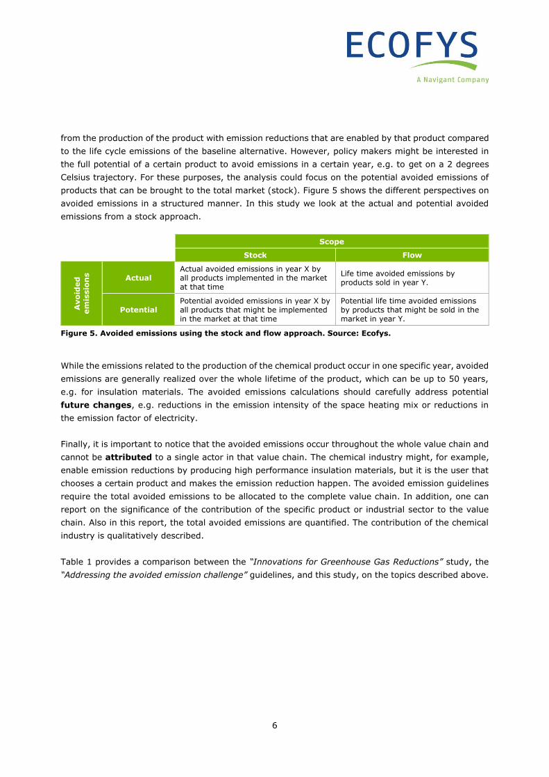
products that can be brought to the total market (stock). Figure 5 shows the different perspectives on
avoided emissions in a structured manner. In this study we look at the actual and potential avoided
emissions from a stock approach.
Scope
Stock Flow
Avo
ided
em
issio
ns
Actual Actual avoided emissions in year X by all products implemented in the market at that time
Life time avoided emissions by products sold in year Y.
Potential Potential avoided emissions in year X by all products that might be implemented in the market at that time
Potential life time avoided emissions by products that might be sold in the market in year Y.
Figure 5. Avoided emissions using the stock and flow approach. Source: Ecofys.
While the emissions related to the production of the chemical product occur in one specific year, avoided
emissions are generally realized over the whole lifetime of the product, which can be up to 50 years,
e.g. for insulation materials. The avoided emissions calculations should carefully address potential
future changes, e.g. reductions in the emission intensity of the space heating mix or reductions in
the emission factor of electricity.
Finally, it is important to notice that the avoided emissions occur throughout the whole value chain and
cannot be attributed to a single actor in that value chain. The chemical industry might, for example,
enable emission reductions by producing high performance insulation materials, but it is the user that
chooses a certain product and makes the emission reduction happen. The avoided emission guidelines
require the total avoided emissions to be allocated to the complete value chain. In addition, one can
report on the significance of the contribution of the specific product or industrial sector to the value
chain. Also in this report, the total avoided emissions are quantified. The contribution of the chemical
industry is qualitatively described.
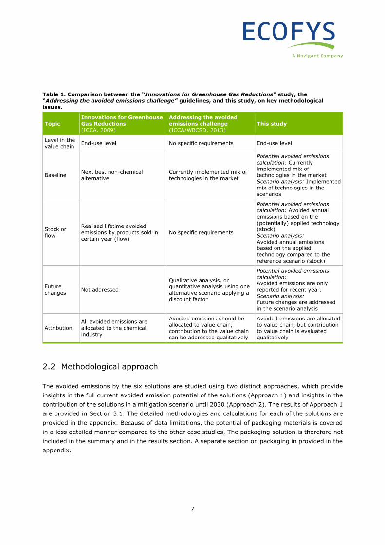
Table 1 provides a comparison between the “Innovations for Greenhouse Gas Reductions” study, the
“Addressing the avoided emission challenge” guidelines, and this study, on the topics described above.
7
Table 1. Comparison between the “Innovations for Greenhouse Gas Reductions” study, the “Addressing the avoided emissions challenge” guidelines, and this study, on key methodological issues.
Topic Innovations for Greenhouse Gas Reductions (ICCA, 2009)
Addressing the avoided emissions challenge (ICCA/WBCSD, 2013)
This study
Level in the value chain
End-use level No specific requirements End-use level
Baseline Next best non-chemical alternative
Currently implemented mix of technologies in the market
Potential avoided emissions calculation: Currently implemented mix of technologies in the market Scenario analysis: Implemented mix of technologies in the scenarios
Stock or flow
Realised lifetime avoided emissions by products sold in certain year (flow)
No specific requirements
Potential avoided emissions calculation: Avoided annual emissions based on the (potentially) applied technology (stock) Scenario analysis: Avoided annual emissions based on the applied technology compared to the reference scenario (stock)
Future changes
Not addressed
Qualitative analysis, or quantitative analysis using one alternative scenario applying a discount factor
Potential avoided emissions calculation: Avoided emissions are only reported for recent year. Scenario analysis: Future changes are addressed in the scenario analysis
Attribution All avoided emissions are allocated to the chemical industry
Avoided emissions should be allocated to value chain, contribution to the value chain can be addressed qualitatively
Avoided emissions are allocated to value chain, but contribution to value chain is evaluated qualitatively
2.2 Methodological approach
The avoided emissions by the six solutions are studied using two distinct approaches, which provide
insights in the full current avoided emission potential of the solutions (Approach 1) and insights in the
contribution of the solutions in a mitigation scenario until 2030 (Approach 2). The results of Approach 1
are provided in Section 3.1. The detailed methodologies and calculations for each of the solutions are
provided in the appendix. Because of data limitations, the potential of packaging materials is covered
in a less detailed manner compared to the other case studies. The packaging solution is therefore not
included in the summary and in the results section. A separate section on packaging in provided in the
appendix.
8
The results of Approach 2 are provided in Section 3.2, which contains four factsheets:
1. Wind and solar power
2. Efficient building envelopes
3. Efficient lighting
4. Fuel efficient tires, lightweight materials and electric cars.
The factsheets highlight the background of the solutions and the contribution of the solutions in the
mitigation scenario. More detailed methodologies and calculations are also provided in the appendix.
2.2.1 Current avoided emissions potential (Approach 1)
To showcase the avoided emissions potential of the solutions to which chemical products contributes, we
quantify the emissions that would be avoided if each selected solution was used to its full potential right
now. We analyse the maximum theoretical use of the solution and quantify how much lower the emissions
would be if this was the case, keeping everything else the same. In addition, we quantify the contribution
the solution currently makes through its current market share. We calculate the contribution the solution
currently makes by calculating how much higher the emissions would be if the solution was not be used
at all. The potential avoided emissions calculation assumes that it would be possible to realise an
immediate 100% implementation of the alternative solution, and is intended to illustrate the possibilities.
The authors realize that this potential is hypothetical and not achievable in a short timeframe and under
the given boundary conditions (e.g. limited availability of raw materials, production capacity and
infrastructure).
The potential avoided emissions (the first approach as outlined in Section 2.1) are calculated using a
bottom-up approach. The avoided emissions potential and realized avoided emissions are analysed by
comparing the emissions of the complete life cycle for a situation without the implementation of the
solution using chemical products at all (“No implementation”), a situation that represents the current
market average of the solution (“Current implementation”) and a situation in which the solution using
chemical products is applied to its maximum potential (“Maximum implementation”). The difference
between the situation without the solution using chemical products and the situation that represents
the market average are the realized avoided emissions by the chemical product. The difference between
the market average and the full potential are the avoided emissions potential. The avoided emissions
are described as net avoided emissions, consisting of increased emissions resulting from the production
of the solution and avoided emissions in the use phase. The avoided emissions in the use phase typically
exceed the production emissions significantly. In analysing the life cycles in the three situations, a
simplified calculation methodology is applied, which means that similar life cycle stages are omitted
from the analysis.
The global potential for avoided emissions of each of the solutions is summarized in Section 3.1. A
detailed description of the methodology and the results of the avoided emissions potential calculation
are provided in the appendix. The detailed results are presented in the appendix with two graphs
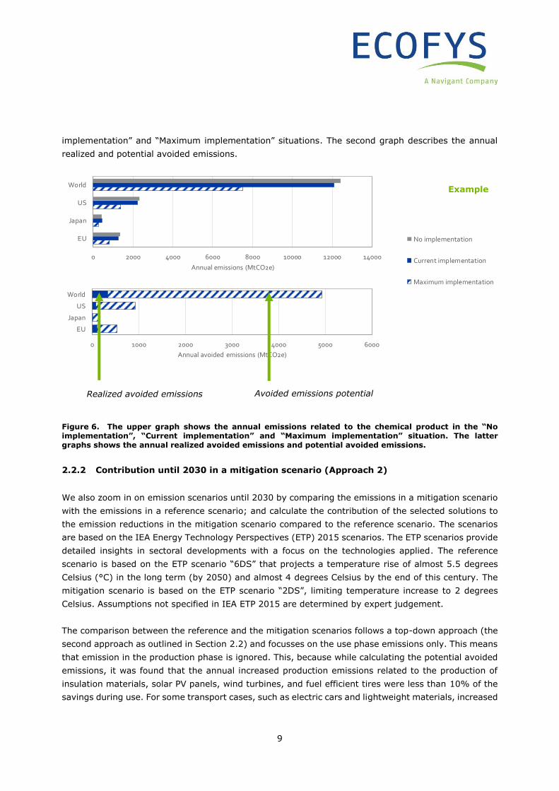
(Figure 6). The first graph describes the total annual emissions in the “No implementation”, “Current
9
implementation” and “Maximum implementation” situations. The second graph describes the annual
realized and potential avoided emissions.
Figure 6. The upper graph shows the annual emissions related to the chemical product in the “No implementation”, “Current implementation” and “Maximum implementation” situation. The latter graphs shows the annual realized avoided emissions and potential avoided emissions.
2.2.2 Contribution until 2030 in a mitigation scenario (Approach 2)
We also zoom in on emission scenarios until 2030 by comparing the emissions in a mitigation scenario
with the emissions in a reference scenario; and calculate the contribution of the selected solutions to
the emission reductions in the mitigation scenario compared to the reference scenario. The scenarios
are based on the IEA Energy Technology Perspectives (ETP) 2015 scenarios. The ETP scenarios provide
detailed insights in sectoral developments with a focus on the technologies applied. The reference
scenario is based on the ETP scenario “6DS” that projects a temperature rise of almost 5.5 degrees
Celsius (°C) in the long term (by 2050) and almost 4 degrees Celsius by the end of this century. The
mitigation scenario is based on the ETP scenario “2DS”, limiting temperature increase to 2 degrees
Celsius. Assumptions not specified in IEA ETP 2015 are determined by expert judgement.
The comparison between the reference and the mitigation scenarios follows a top-down approach (the
second approach as outlined in Section 2.2) and focusses on the use phase emissions only. This means
that emission in the production phase is ignored. This, because while calculating the potential avoided
emissions, it was found that the annual increased production emissions related to the production of
insulation materials, solar PV panels, wind turbines, and fuel efficient tires were less than 10% of the
savings during use. For some transport cases, such as electric cars and lightweight materials, increased
0 2000 4000 6000 8000 10000 12000 14000
EU
Japan
US
World
Annual emissions (MtCO2e)
Electricity from wind and solar
No implementation
Current implementation
Maximum implementation
0 1000 2000 3000 4000 5000 6000
EU
Japan
US
World
Annual avoided emissions (MtCO2e)
Realized avoided emissions Avoided emissions potential
Example
10
production emissions can be more substantial as result of the high emissions related to the production
of batteries and lightweight materials, such as carbon fibre reinforced plastics, increasing the
uncertainty of the avoided emissions calculation.
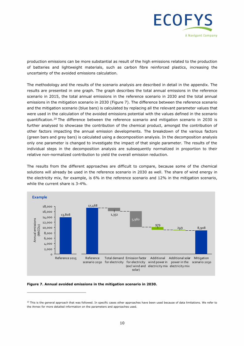
The methodology and the results of the scenario analysis are described in detail in the appendix. The
results are presented in one graph. The graph describes the total annual emissions in the reference
scenario in 2015, the total annual emissions in the reference scenario in 2030 and the total annual
emissions in the mitigation scenario in 2030 (Figure 7). The difference between the reference scenario
and the mitigation scenario (blue bars) is calculated by replacing all the relevant parameter values that
were used in the calculation of the avoided emissions potential with the values defined in the scenario
quantification.20 The difference between the reference scenario and mitigation scenario in 2030 is
further analysed to showcase the contribution of the chemical product, amongst the contribution of
other factors impacting the annual emission developments. The breakdown of the various factors
(green bars and grey bars) is calculated using a decomposition analysis. In the decomposition analysis
only one parameter is changed to investigate the impact of that single parameter. The results of the
individual steps in the decomposition analysis are subsequently normalized in proportion to their
relative non-normalized contribution to yield the overall emission reduction.
The results from the different approaches are difficult to compare, because some of the chemical
solutions will already be used in the reference scenario in 2030 as well. The share of wind energy in
the electricity mix, for example, is 6% in the reference scenario and 12% in the mitigation scenario,
while the current share is 3-4%.
Figure 7. Annual avoided emissions in the mitigation scenario in 2030.
20 This is the general approach that was followed. In specific cases other approaches have been used because of data limitations. We refer to
the Annex for more detailed information on the parameters and approaches used.
Example
8,908249979
1,352
17,468
5,980
Reference scenario 2030
Mitigation scenario 2030
Additional solar power in the
electricity mix
Additional wind power in electricity mix
Emission factor for electricity (excl wind and
solar)
Total demand for electricity
16,000
14,000
12,000
18,000
10,000
8,000
6,000
4,000
2,000
0
An
nu
al e
mis
sio
ns
(MtC
O2
)
Reference 2015
13,808
11
2.2.3 Limitations of the approach
Across the case studies there can be uncertainties about specific assumptions, including the current
market share (e.g. the current share of green tires), regional information (e.g. the average U values),
efficiency improvement factors (e.g. lightweight materials for the automotive industry), both related to
the state of art, as well to potential future developments (e.g. future efficiency improvement of LED
light bulbs).
In view of the typical uncertainties related to the type of calculations it should be stressed that the avoided
emission potentials presented in his study are to be viewed as approximate values. As an example, a
sensitivity analysis in building envelopes shows that a potential for avoided emissions ranges between
0.5 GtCO2e and 1.3 GtCO2e, while maximum avoided emissions is estimated to be 1.2 GtCO2e.
12
Results
The avoided emissions potential of the six quantified solutions together is presented in Section 3.1
and showcase the emissions that would have been avoided if the selected solution would have been
used to its full potential right now. The emission scenarios are described case by case in the
factsheets included in Section 3.2.
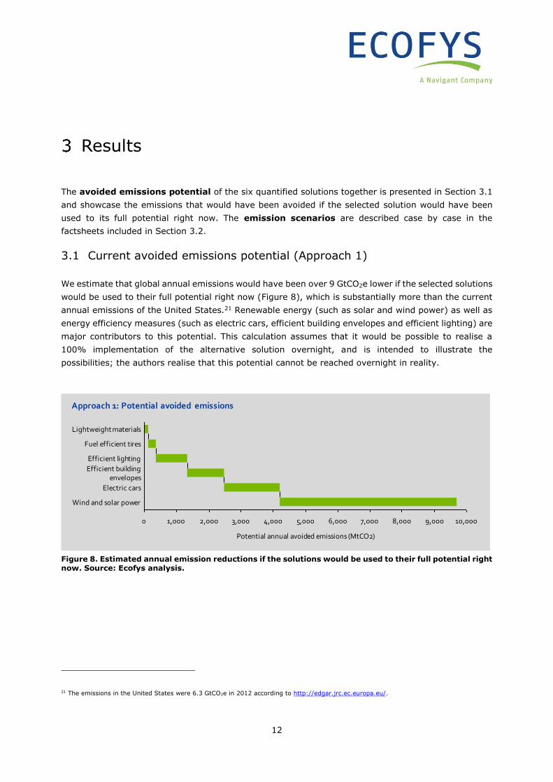
3.1 Current avoided emissions potential (Approach 1)
We estimate that global annual emissions would have been over 9 GtCO2e lower if the selected solutions
would be used to their full potential right now (Figure 8), which is substantially more than the current
annual emissions of the United States.21 Renewable energy (such as solar and wind power) as well as
energy efficiency measures (such as electric cars, efficient building envelopes and efficient lighting) are
major contributors to this potential. This calculation assumes that it would be possible to realise a
100% implementation of the alternative solution overnight, and is intended to illustrate the
possibilities; the authors realise that this potential cannot be reached overnight in reality.
Figure 8. Estimated annual emission reductions if the solutions would be used to their full potential right now. Source: Ecofys analysis.
21 The emissions in the United States were 6.3 GtCO2e in 2012 according to http://edgar.jrc.ec.europa.eu/.
Approach 1: Potential avoided emissions
0 1,000 2,000 3,000 4,000 5,000 6,000 7,000 8,000 9,000 10,000
Wind and solar power
Lightweight materials
Electric cars
Fuel efficient tires
Efficient buildingenvelopes
Efficient lighting
Potential annual avoided emissions (MtCO2)
13
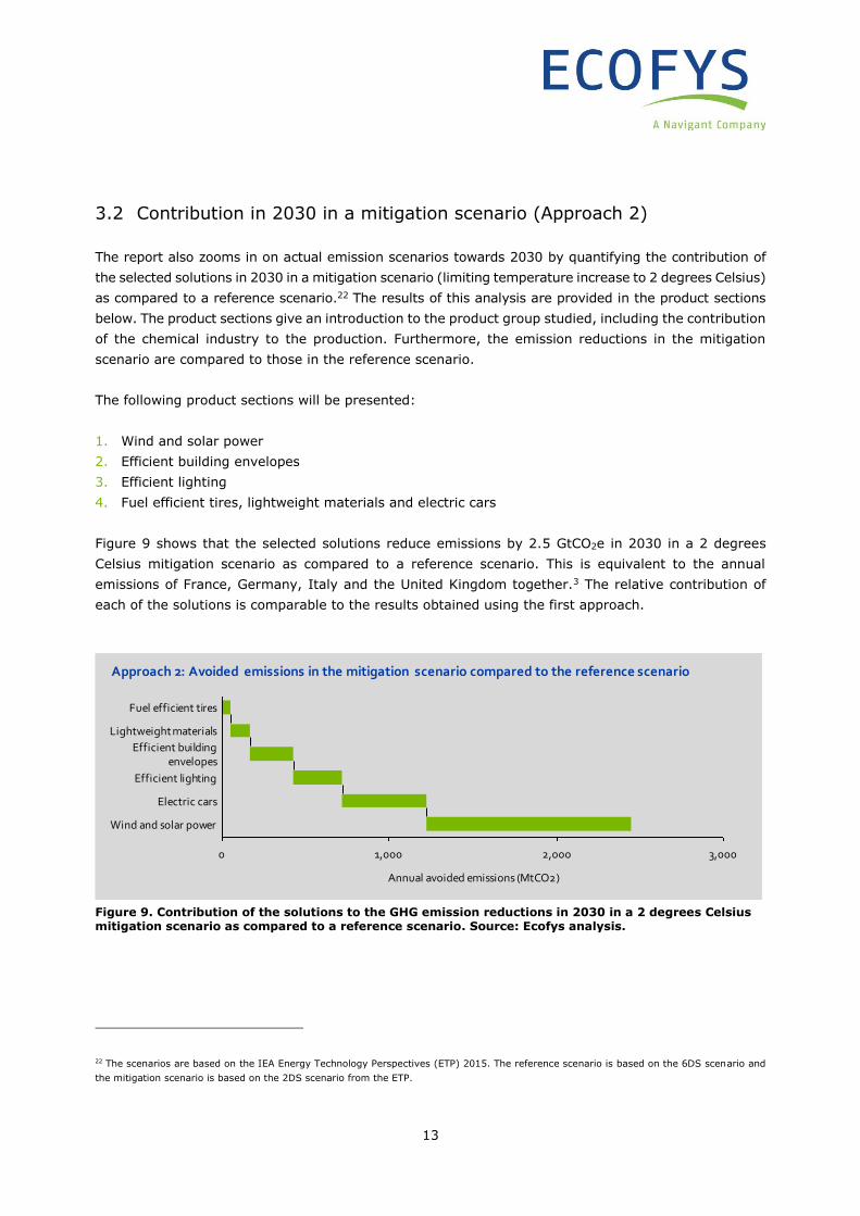
3.2 Contribution in 2030 in a mitigation scenario (Approach 2)
The report also zooms in on actual emission scenarios towards 2030 by quantifying the contribution of
the selected solutions in 2030 in a mitigation scenario (limiting temperature increase to 2 degrees Celsius)
as compared to a reference scenario.22 The results of this analysis are provided in the product sections
below. The product sections give an introduction to the product group studied, including the contribution
of the chemical industry to the production. Furthermore, the emission reductions in the mitigation
scenario are compared to those in the reference scenario.
The following product sections will be presented:
1. Wind and solar power
2. Efficient building envelopes
3. Efficient lighting
4. Fuel efficient tires, lightweight materials and electric cars
Figure 9 shows that the selected solutions reduce emissions by 2.5 GtCO2e in 2030 in a 2 degrees
Celsius mitigation scenario as compared to a reference scenario. This is equivalent to the annual
emissions of France, Germany, Italy and the United Kingdom together.3 The relative contribution of
each of the solutions is comparable to the results obtained using the first approach.
Figure 9. Contribution of the solutions to the GHG emission reductions in 2030 in a 2 degrees Celsius mitigation scenario as compared to a reference scenario. Source: Ecofys analysis.
22 The scenarios are based on the IEA Energy Technology Perspectives (ETP) 2015. The reference scenario is based on the 6DS scenario and
the mitigation scenario is based on the 2DS scenario from the ETP.
Approach 2: Avoided emissions in the mitigation scenario compared to the reference scenario
0 1,000 2,000 3,000
Annual avoided emissions (MtCO2)
Electric cars
Efficient buildingenvelopes
Efficient lighting
Lightweight materials
Fuel efficient tires
Wind and solar power
14
Wind and solar power
Renewable and low carbon electricity, such as wind and solar power, play a key role in the
decarbonisation of our energy system. The chemical industry contributes to the deployment
of renewables through the supply of key materials for wind turbines and solar PV panels,
including gear oils for wind turbine gearboxes, resins for blades and coating materials for
wind turbines, and silicon ingots, semiconductor gas and sealant for PV panels. A higher
share of renewable energy as result of additional wind and solar power in the electricity mix
contributes to over 1200 MtCO2e of emission reductions in the mitigation scenario as
compared to the reference scenario.
Renewable electricity is key in the decarbonisation of the energy system. In all scenarios from the
Energy Technology perspectives, installed capacities for electricity production from biomass, hydro,
geothermal, wind, solar and ocean will increase. In the 6DS scenario the installed renewable capacity
increases to over 3000 GW in 2030. In the 2DS scenario the capacity increases to over 4500 GW in
2030.23 The share of wind and solar in the electricity mix increases from about 3.5% and 1.0% in 2015
to 5-12% and 2-4% in the various scenarios in 2030.24 The chemical industry contributes to the
deployment of wind and solar power through the supply of key materials for wind turbines and solar
PV panels, such as gear oils for wind turbine gearboxes, resins for wind turbine blades, and silicon
ingots for PV panels. Emissions related to the production of wind turbines and solar PV panels are small
(< 5%) compared to the emission reduction achieved.
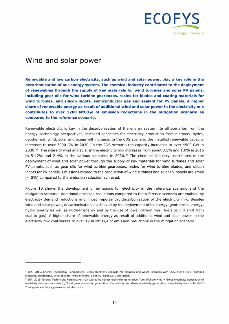
Figure 10 shows the development of emissions for electricity in the reference scenario and the
mitigation scenario. Additional emission reductions compared to the reference scenario are enabled by
electricity demand reductions and, most importantly, decarbonisation of the electricity mix. Besides
wind and solar power, decarbonisation is achieved by the deployment of bioenergy, geothermal energy,
hydro energy as well as nuclear energy and by the use of lower carbon fossil fuels (e.g. a shift from
coal to gas). A higher share of renewable energy as result of additional wind and solar power in the
electricity mix contributes to over 1200 MtCO2e of emission reductions in the mitigation scenario.
23 IEA, 2015. Energy Technology Perspectives. Gross electricity capacity for biomass and waste, biomass with CCS, hydro (excl. pumped
storage), geothermal, wind onshore, wind offshore, solar PV, solar CSP, and ocean. 24 IEA, 2015. Energy Technology Perspectives. Calculated by (Gross electricity generation from offshore wind + Gross electricity generation of
electricity from onshore wind) / Total gross electricity generation of electricity and Gross electricity generation of electricity from solar PV) /
Total gross electricity generation of electricity
15
Figure 10. Annual avoided emissions from additional wind and solar power in the mitigation scenario in 2030. Source: Ecofys analysis based on ETP scenarios.
More details on the avoided emissions potential and the scenario analysis can be found in Section 5.2.
Wind and solar power
8,908249979
1,352
17,468
5,980
Reference scenario 2030
Mitigation scenario 2030
Additional solar power in the
electricity mix
Additional wind power in electricity mix
Emission factor for electricity (excl. additional
wind and solar power)
Total demand for electricity
16,000
14,000
12,000
18,000
10,000
8,000
6,000
4,000
2,000
0
An
nu
al e
mis
sio
ns
of
the
po
wer
sec
tor
(MtC
O2
)
Reference 2015
13,808
16
Efficient building envelopes
Emissions related to space heating of buildings represent a significant share of global GHG
emissions. Deep renovation could result in energy efficiency improvements up to 80% in
existing buildings. The chemical industry contributes to deep renovation through the
production of wall and roof insulation materials like expanded polystyrene (EPS) and
polyurethane (PUR), or key components of windows and doors. The annual emission
reduction from additional residential efficient building envelopes including additional
insulation in the mitigation scenario will amount to over 250 MtCO2e in 2030 as compared
to the reference scenario.
Emissions related to both residential and commercial buildings represent a significant share of global
GHG emissions. Over 6% of global GHG emissions are directly emitted by the building sector and
buildings are also responsible for a further 12% of global emissions resulting from indirect emissions.25
The IEA recommends member countries to focus on both deep energy renovations of the existing
building stock and on strict building codes for new building, with the eventual goal of near zero or zero
energy buildings.26
Studies on reducing energy consumption and emissions from heating and cooling (which are
responsible for 36% of global building energy consumption27) are numerous including the IEA study on
the “Transition to Sustainable Buildings”, work by the Global Building Performance Network (GBPN),
and regional work such as the studies done by Ecofys for the European insulation industry.26,26,28
Although the studies obviously differ in scope and set-up, conclusions are often similar pointing at the
low or even negative costs of many of the mitigation options available and the many co-benefits and
the existence of strong barriers (e.g. related to upfront investment needs). The need for high
performance retrofit as mitigation strategy is also highlighted.25
Avoided emissions from building envelope improvement and energy efficiency in the residential building
sector are dominated by the reduction in heating fuel consumption during the use phase. Deep
renovation could result in energy efficiency improvements up to 80% in existing buildings. The
25 IPCC, 2014. Climate Change 2014: Mitigation of Climate Change. Contribution of Working Group III to the Fifth Assessment Report of the
Intergovernmental Panel on Climate Change. Chapter 9: Buildings. According to IPCC (2014) the GHG emissions from the buildings sector
reached over 9 GtCO2e in 2010, representing 19% of all global GHG emissions. One third is related to direct emissions and two third is related
to indirect emissions. Indirect emissions are emissions related to electricity use and (district) heat consumption. 26 IEA, 2013. Transition to Sustainable Buildings. Strategies and Opportunities to 2050. 27 According to IPCC, 2014, the final energy consumption for space heating and cooling amount to 32% and 4% in the residential sector and
33% and 7% in the commercial sector. Other large categories are water heating (24%) and cooling (29%) in the residential buildings. and
lighting (16%) and other (including IT equipment) (32%) in the commercial buildings. In cold climates the share of space heating can be
substantially higher. 28 Ecofys, 2012. Renovation Tracks for Europe up to 2050. Available at: http://www.ecofys.com/en/publication/renovation-tracks-for-europe-
up-to-2050.
17
chemical industry contributes to deep renovation through the production of insulation materials like
EPS and PUR. The chemical industry, together with competing insulation materials such as rock and
glass wool), is of essential importance in tapping the CO2 emissions related to the existing building
stock, which can result in CO2 savings of up to 80-90%.28 Emissions related to the production of the
insulation material are marginal compared to the use phase emissions.
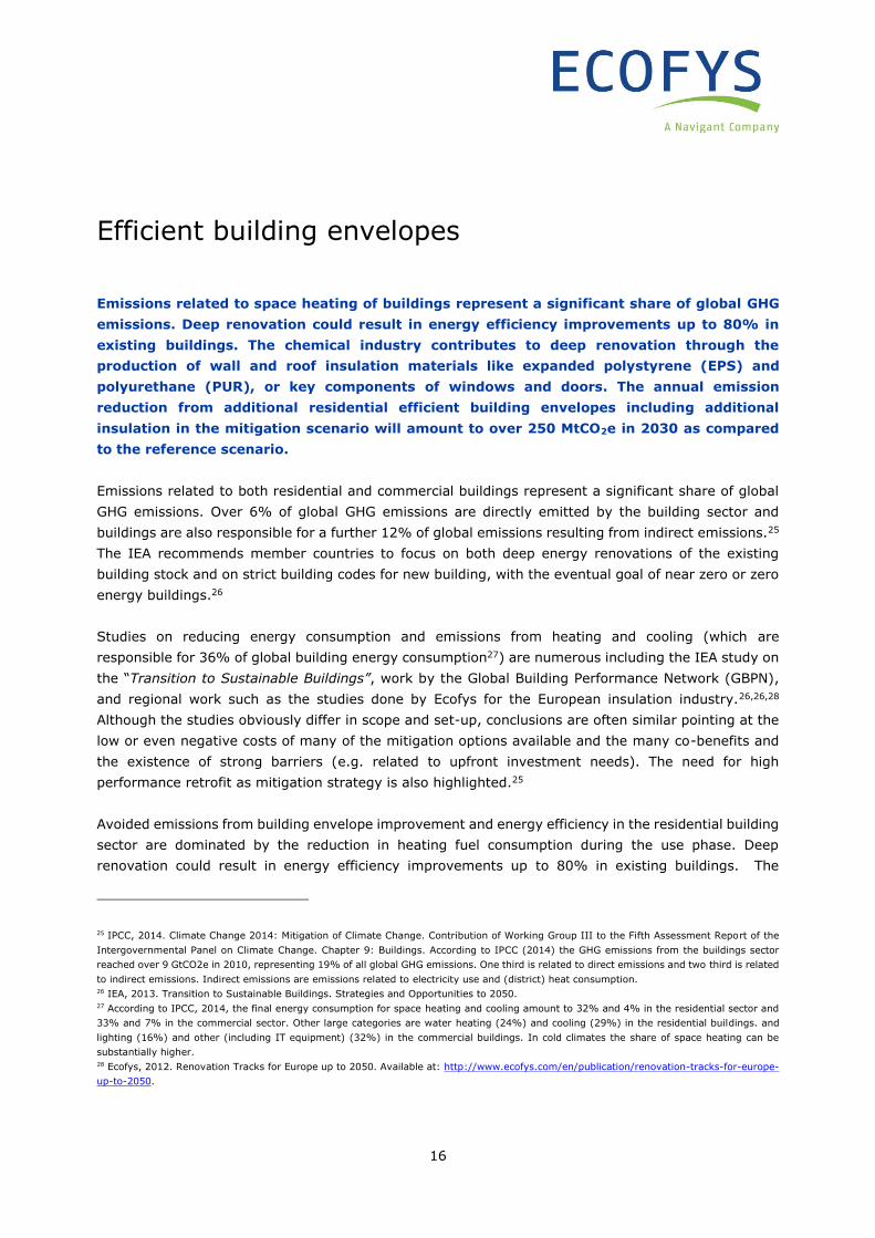
Figure 11 shows the development of emissions for residential space heating in the reference scenario
and the mitigation scenario. Additional emission reductions compared to the reference scenario are
enabled by building envelope improvements,29 as well as a reduction in the carbon intensity for space
heating. The annual emission reduction from additional efficient building envelopes including additional
insulation in the mitigation scenario will amount to over 250 MtCO2e in 2030. In addition, improving
the energy efficiency of buildings has a lot of co-benefits beyond climate change mitigation, such as
increased comfort levels.
Figure 11. Annual avoided emissions from additional residential efficient building envelopes in the mitigation scenario in 2030. Source: Ecofys analysis based on ETP scenarios.
More details on the avoided emissions potential and the scenario analysis can be found in Section 5.3.
29 Building envelope improvements include, amongst other, improve floor, wall and roof insulation, efficient windows and efficient technologies
used for energy conversion.
Efficient building envelopes
1,401
2,006
345
260
Mitigation scenario 2030
Carbon intensity for space heating
Building envelope improvement
Reference scenario 2030
0
500
2,500
2,000
1,500
1,000
Reference 2015
1,692
An
nu
al e
mis
sio
ns
fro
m r
esid
enti
al s
pac
e h
eati
ng
(MtC
O2
)
18
Efficient lighting
Substantial opportunities exist to improve the energy efficiency of appliances in buildings.
LED (light-emitting diode) light bulbs are new and highly energy efficient light bulbs, that
have a much higher luminous efficiency than conventional light bulbs such as incandescent
bulbs and halogen bulbs. The energy efficiency potential of LED light bulbs is up to 80%
compared to what is currently applied in the market. Chemical products, such as
semiconductor gas, phosphor, substrate, and sealant, are essential materials to enable high
energy efficiency, reliability, and long life of LED light bulbs. Energy efficiency improvement
as a result of additional efficient lighting will contribute to an annual emission reduction of
approximately 300 MtCO2e in 2030 as compared to the reference scenario.
Global emissions related to lighting in buildings were over 1000 MtCO2e in 2015. While LED light bulbs
have much higher luminous efficiency that other light bulbs, their current market penetration is rather
limited. Increasing market penetration and further energy efficiency improvement will result in
substantial emission reductions. The energy efficiency potential of LED light bulbs is up to 80%
compared to what is currently applied in the market.30 Chemical products, such as semiconductor gas,
phosphor, substrate, and sealant, are essential materials to enable high energy efficiency, reliability,
and long life of LED light bulbs. Without these newly developed materials for LED, performance of LED
would have been much lower than the current level.
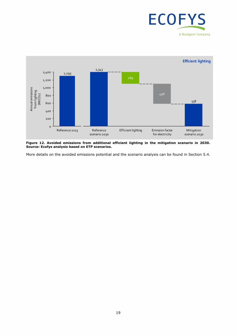
Figure 12 shows the development of emissions for lighting in the reference scenario and the mitigation
scenario. Emission reductions are enabled by deployment of energy efficient lighting, such as LED
lamps, as well as decarbonisation of the electricity mix. Energy efficiency improvement as a result of
additional efficient lighting will contribute to an annual emission reduction of approximately 300 MtCO2e
in 2030. Deployment of LED light bulbs has a lot of co-benefits beyond climate change mitigation,
including a reduction of life cycle costs for lighting compared to conventional light bulbs and an
improved safety compared to kerosene lighting in developing countries.
30 Calculated based on a current average luminous efficiency of 30 lm/W, compared to a LED luminous efficiency of 150 lm/W, which represent
the current state-of-art technology.
19
Figure 12. Avoided emissions from additional efficient lighting in the mitigation scenario in 2030. Source: Ecofys analysis based on ETP scenarios.
More details on the avoided emissions potential and the scenario analysis can be found in Section 5.4.
Efficient lighting
558
1,343
496
289
Reference scenario 2030
Efficient lighting Mitigation scenario 2030
Emission factor for electricity
1,400
1,000
1,200
800
400
200
0
600
An
nu
al e
mis
sio
ns
fro
m li
gh
tin
g(M
tCO
2)
1,295
Reference 2015
20
Fuel efficient tires, lightweight materials and
electric cars
Multiple options to reduce GHG emissions in the road transport sector need to be tapped to
address climate change. Emission reductions can be enabled by transport demand
reductions, but also by efficient technologies, such as fuel efficient tires, lightweight
materials and electric cars. The emission reduction potential of fuel efficient tires in the
mitigation scenario amounts to over 50 MtCO2e in 2030, the emission reduction potential of
lightweight materials amounts to over 100 MtCO2e and the emission reduction potential of
electric cars amounts to over 500 MtCO2e, all as compared to the reference scenario.
Road transport (including cars, busses, and trucks) accounts for more than two third of the final energy
consumption for transport.31 Roughly 20% of automobiles' fuel consumption is used to overcome rolling
resistance of the tires.32 Fuel efficient tires have lower rolling resistance compared to normal tires,
while providing enhanced road-gripping performance, resulting in an energy efficiency improvement of
about 2.5%.33 Chemical products such as synthetic rubbers and silica are key components in reducing
energy loss and enabling improved fuel efficiency of tires. Application of additional fuel efficient tires
will contribute to an annual emission reduction of over 50 MtCO2e in 2030.
Electrification of road transport enables deep decarbonisation of the energy demand when renewable
electricity is supplied on a large scale. Furthermore, electric cars have a higher energy efficiency
compared to cars with conventional combustion engines. Chemical products play a key role in the
production of batteries required for electric cars. These include anode materials, cathode materials,
electrolyte and separators. More electric cars in the mitigation scenario will contribute to an annual
emission reduction of more than 500 MtCO2e in 2030.
Lightweight materials reduce the fuel demand of cars. Innovative lightweight materials have the
potential to reduce car weight substantially. However, historically, car weight is rather constant as a
result of higher safety requirements, bigger cars, and more appliances. Chemical products such as
plastics and carbon fiber reinforced plastics are key in achieving strong weight reductions of cars.
Additional lightweight materials in the mitigation scenario will contribute to an annual emission
reduction of more than 100 MtCO2e in 2030.
31 Final energy consumption for road transport for passengers and freight account for 80 EJ compared a total final energy consumption for
transport of 103 EJ in 2012 according to IEA, 2015. Energy Technology Perspectives. 32 IEA, 2005. Energy Efficient Tyres: Improving the On-Road Performance of Motor Vehicles, IEA Workshop, 15-16 November 2005, OECD/IEA,
Paris, www.iea.org/work/2005/EnerEffTyre/summary.pdf. 33 ICCA/JCIA, 2015. Case Study: Materials for Fuel Efficient Tires. Available at: http://www.icca-chem.org/Public/Avoided%20Emissions%20
Case%20Studies/Case%20study%201%20-%20Avoided%20Emissions%20Guideline%20-%20JCIA.pdf
21
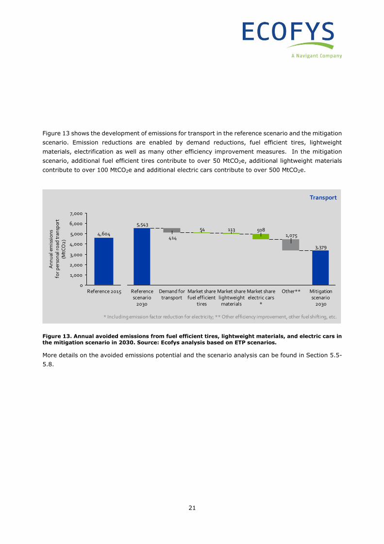
Figure 13 shows the development of emissions for transport in the reference scenario and the mitigation
scenario. Emission reductions are enabled by demand reductions, fuel efficient tires, lightweight
materials, electrification as well as many other efficiency improvement measures. In the mitigation
scenario, additional fuel efficient tires contribute to over 50 MtCO2e, additional lightweight materials
contribute to over 100 MtCO2e and additional electric cars contribute to over 500 MtCO2e.
Figure 13. Annual avoided emissions from fuel efficient tires, lightweight materials, and electric cars in the mitigation scenario in 2030. Source: Ecofys analysis based on ETP scenarios.
More details on the avoided emissions potential and the scenario analysis can be found in Section 5.5-
5.8.
Transport
3,379
1,07550811354
414
5,543
Mitigation scenario
2030
Market share electric cars
*
Other**Demand for transport
Reference scenario
2030
Market share fuel efficient
tires
Market share lightweight
materials
3,000
2,000
7,000
6,000
4,000
5,000
1,000
0Reference 2015
4,604
An
nu
al e
mis
sio
ns
for
per
son
al r
oad
tran
spor
t(M
tCO
2)
* Including emission factor reduction for electricity; ** Other efficiency improvement, other fuel shifting, etc.
22
Conclusion
It is estimated that annual global emissions would be over 9 GtCO2e lower if the selected solutions with
chemical products of fundamental or extensive significance were used to their full potential right now.
This exceeds the current annual emissions of the United States.21 Renewable energy (such as solar and
wind power) as well as energy efficiency measures (such as efficient building envelopes, electric cars
and efficient lighting) are major contributors to this potential. In addition, the contribution the solutions
currently already make through their current market shares was quantified.
The report also zooms in on actual emission scenarios towards 2030 by quantifying the contribution of
the selected solutions in 2030 in a mitigation scenario (limiting temperature increase to 2 degrees Celsius)
as compared to a reference scenario. The study shows that the selected solutions contribute up to
2.5 GtCO2e to the difference between these two scenarios in the year 2030.34 This is equal to 14% of the
total mitigation effort required in 2030 to move from the reference scenario towards the mitigation
scenario and equivalent to the current annual emissions of France, Germany, Italy and the United
Kingdom together.35 In view of the typical uncertainties related to the type of calculations it should be
stressed that the avoided emission potentials presented in his study are to be viewed as indicative only.
Many industrial and other stakeholders work together for each of the studied solutions. Enhanced value
chain cooperation is needed to fully exploit the potential. The chemical industry is, for example, committed
to providing energy efficient solutions to the buildings sector, by efforts such as participation in pilot
projects, sponsoring life cycle assessment studies, investments in research and development, and
cooperation with the value chain; from architects to craftsmen.36
An enabling policy environment is needed, stimulating greenhouse gas emission reductions along the full
value chain, including use and end-of life phases.
• Governments should establish technology neutral policies which enable cost effective renewable
energy to grow and contribute to greenhouse gas emission reductions, while ensuring the reliable,
affordable, and non-intermittent supply of electricity. Financial support should only be available for
research and technology development of pre-commercial innovative technologies. All technologies
should be integrated into normal market conditions, removing subsidies as soon as the technology is
commercial.
34 It should be noted the use of some of the chemical solutions will increase also in the reference scenario in 2030 as compared to the situation
nowadays. Part of the potential identified following the first approach will thus also already be tapped in the reference scenario. 35 The mitigation effort according to the IEA ETP scenarios (6DS versus 2DS) is 17.2 GtCO2e according to IEA, 2015. Energy Technology
Perspectives, Figure 1.6. The emissions of France, Germany, Italy and the United Kingdom were 2.5 GtCO2e in 2012 according to
http://edgar.jrc.ec.europa.eu/. 36 ICCA, 2015. ICCA Building Technology Roadmap: The Chemical Industry’s Contributions to Energy and Greenhouse Gas Savings in
Residential and Commercial Construction. Executive summary available at: https://www.icca-chem.org/wp-content/uploads/2015/08/ICCA-
Building-Technology-Roadmap-Executive-Summary.pdf.
23
• Energy efficient measures have a large potential of saving energy and reducing greenhouse gas
emissions worldwide. Governments should, for example, set energy efficiency standards, encourage
manufacturers to provide correct and easy-to-understand information, and take necessary actions to
raise public awareness depending on regional/national circumstances.
Further work is needed, also by the modelling teams, to shed more light on the exact impact mitigation
will have on the material demand and resulting emissions of the chemical industry itself; a somewhat
unexplored issue in the current modelling due to the focus on the use phase of emissions in the scenario
work.
The selected solutions highlight the opportunities of the chemical industry in a low carbon world. The
chemical industry has the potential to contribute even more and to further accelerate its contribution also
beyond the 2030 timeframe. For all solutions to be used widely, joint action from all partners in the value
chain is needed, as well as different business models, supported by a sufficiently enabling policy conditions
at an adequate level.
24
Appendix
This appendix provides the detailed methodology and calculations for the seven solutions studied. In
Section 5.1 the emission factors used in the potential avoided emissions calculation are described. In
Section 5.2 to 5.9 the case studies are described. The case study descriptions contain an overview of
the contribution of the chemical industry toward this solution, the methodology and calculation details
for the potential avoided emissions and the methodology and calculation details for the scenario
analysis. Finally, the references used in the case studies are provided.
5.1 Emission factors
In Section 5.1.1 and Section 5.1.2 the direct and life cycle emission factors for fuels, heat and electricity
are provided for various regions in the world. These factors are used in the potential avoided emissions
calculations for the case studies. Direct emissions are those emissions related to solely the combustion
of fuels at the generation facility. Life cycle emissions include emissions related to all other activities in
the life cycle, e.g. raw material extraction, power plant construction, power plant maintenance and
waste disposal. Note that the direct emission factors of electricity and heat differ per region due to a
different heat (Ecofys/IEE Japan, 2015) and electricity mix (IEA, 2014). The emission factors of
electricity are highly dependent on the fuel mix. As result of generation inefficiencies and a limited
share of renewables in the energy mix, the emission factors of electricity generation are generally
higher per kWh of electricity compared to those for the combustion of fossil fuels per kWh of fuel. The
indirect emissions (life cycle emissions excluding direct emissions) are assumed to be the same for
different regions. The life cycle emission factors are calculated by multiplying the direct emission factors
with an indirect emission correction factor.37
37 The indirect emission correction factors are calculated based on the energy requirements for energy, which describe the primary energy
that is required to extract and deliver one unit of energy. The following values are used for coal: 1.07, gas/diesel/fuel oil: 1.12, kerosene:
1.12, natural gas: 1.03, LPG/natural gas liquids: 1.03, heat: 1, geothermal: 1, combustion renewable and waste: 1, electricity: 1.19. The
indirect emission correction factor for coal, oil products and natural gas are based on ranges provided in Blok (2007). The indirect emission
correction factor for electricity is calculated on a rough estimate of the shares of coal (40%), oil (4%) and natural gas (22%) in the global
electricity mix, in combination with information on the direct and indirect emissions in following Ecoinvent processes: Hard coal, burned in
power plant/NORDEL U (direct: 0.094, total: 0.113, ratio: 1,20), Heavy fuel oil, burned in power plant/RER U (direct: 0.079, total: 0.080,
ratio: 1.015) and Natural gas, burned in power plant/UCTE U (direct: 0.045, total: 0.068, ratio: 1.218). The life cycle emission factor for
electricity is generally higher compared to the life cycle emission factor for burning fossil fuels, because electricity production requires, beside
infrastructure for fossil fuel extraction, also infrastructure for electricity generation. For heat, geothermal and combustion renewable and waste
the correction factor is assumed to be 1.
25
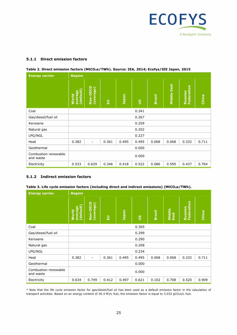
5.1.1 Direct emission factors
Table 2. Direct emission factors (MtCO2e/TWh). Source: IEA, 2014; Ecofys/IEE Japan, 2015
Energy carrier Region
Wo
rld
averag
e
(d
efa
ult
)
No
n-O
EC
D
(averag
e)
EU
Jap
an
US
Brazil
Mid
dle
East
Ru
ssia
n
Fed
era
tio
n
Ch
ina
Coal 0.341
Gas/diesel/fuel oil 0.267
Kerosene 0.259
Natural gas 0.202
LPG/NGL 0.227
Heat 0.382 - 0.361 0.495 0.495 0.068 0.068 0.332 0.711
Geothermal 0.000
Combustion renewable and waste
0.000
Electricity 0.533 0.629 0.346 0.418 0.522 0.086 0.595 0.437 0.764
5.1.2 Indirect emission factors
Table 3. Life cycle emission factors (including direct and indirect emissions) (MtCO2e/TWh).
Energy carrier Region
Wo
rld
averag
e
(d
efa
ult
)
No
n-O
EC
D
(averag
e)
EU
Jap
an
US
Brazil
Mid
dle
East
Ru
ssia
n
Fed
era
tio
n
Ch
ina
Coal 0.365
Gas/diesel/fuel oil 0.299
Kerosene 0.290
Natural gas 0.208
LPG/NGL 0.234
Heat 0.382 - 0.361 0.495 0.495 0.068 0.068 0.332 0.711
Geothermal 0.000
Combustion renewable and waste
0.000
Electricity 0.634 0.749 0.412 0.497 0.621 0.102 0.708 0.520 0.909
* Note that the life cycle emission factor for gas/diesel/fuel oil has been used as a default emission factor in the calculation of
transport activities. Based on an energy content of 36.4 MJ/L fuel, the emission factor is equal to 3.032 gCO2e/L fuel.
26
5.1.3 References
Blok, 2007. Introduction to Energy Analysis.
IEA, 2014. CO2 Emissions from Fuel Combustion.
Ecofys/IEE Japan, 2015. Development of sectoral indicators for determining potential decarbonisation opportunity.
Available at: http://www.ecofys.com/files/files/ieej-ecofys-2015-development-of-sectoral-indicators.pdf
5.2 Wind and solar power
5.2.1 Contribution of chemical industry
The chemical industry fundamentally or extensively contributes to the deployment of renewables
through the supply of key materials for wind turbines and solar PV panels. The chemical industry
provides key materials to renewable power generation systems, including gear oils for wind turbine
gearboxes, resins for blades and coating materials for wind turbines, and silicon ingots, semiconductor
gas and sealant for PV panels. Besides the contribution to wind and solar power, the chemical industry
can also play a fundamental role in the large scale energy storage required with higher shares of
renewables.
5.2.2 Avoided emissions potential calculation
Functional unit
The selected functional unit is generating worldwide electricity in 2012, which is equal to
22,668,076 GWh (IEA, 2012). The ICCA/WBCSD guidelines state that the solutions to compare shall
deliver the same user function. This implies that when wind and solar energy is compared with fossil-
based energy, which has a full-time availability, wind and solar energy should be backed with an energy
storage system to be comparable. Modelling an entire energy system with storage possibilities is out
of scope for this study. As a result, the decision has been made not to account for energy storage, but
to focus on a realistic potential share of wind and solar electricity generation instead of a technical
potential share. With this simplified approach it is also assumed that the reliability of the electricity
system can be guaranteed with the current installed capacity. The potential avoided emissions are
calculated by the difference in life cycle GHG emissions from an electricity mix with a realistic
percentage of wind and solar and the current electricity mix.
Solutions to compare
Three solutions to compare are analysed, including no implementation, current implementation and
maximum implementation of electricity generation by wind and solar (Table 4). All other energy
sources, like gas, coal, nuclear and hydro are grouped in and referred to as “other energy sources”. In
contrary to other case studies the “maximum implementation” of wind and solar power is considered
to be lower than 100%. This is because electricity generation by solely wind and solar cannot provide
the same system function compared to the current generation mix (security of supply). A fully
renewable electricity mix requires, besides wind and solar generation capacity, also back-up capacity
27
that is not dependent on weather patterns, such as hydropower plants, biofuel plants and storage
facilities. Whereas in other case studies the solution “maximum implementation” is focused on a
technical potential, in this case study the decision has been made to derive the share of wind and solar
from the 450 scenario of the World Energy Outlook for 2040 (OECD/IEA, 2015). The percentage of
renewables in the 450 scenario is based on a 50% probability of limiting the average global temperature
increase to the international goal of below 2 degrees Celsius.
Table 4. Solutions to compare.
Solutions Explanation
No implementation of wind and solar
This represents a hypothetical 2012 situation without wind and solar electricity generation.
Current implementation of wind and solar
This is the present electricity mix in 2012.
Maximum implementation of wind and solar
This represents a hypothetical situation with a maximum share of wind and solar electricity generation in the electricity mix. Assumption based on the World Energy Outlook (OECD/IEA, 2015).
Calculation sequence and key data sources
The avoided emissions are calculated by the difference in the life cycle GHG emissions associated with
generating electricity in 2012 (baseline). Total GHG emissions per solution to compare are calculated
as follows:
• Production and end-of-life phase:
o Calculation of GHG emissions by multiplying the amount of electricity generated by solar,
wind and other energy sources with the production and end-of-life emission factor of wind,
solar and other energy sources per TWh.
• Use phase:
o Calculation of emission factor of the total electricity mix for the three solutions to compare
based on the share of wind, solar and other energy sources:
▪ Starting point is the emission factor of the electricity mix in 2012, which is derived
from the IEA CO2 Emissions database (IEA, 2014).
▪ Calculation of the direct emission factor of “wind”, “solar” and “other energy
sources”. The direct emission factor of “solar” and “wind” is zero. The direct
emission factor of “other energy sources” is calculated based on the emission factor
of the current electricity mix and the shares per energy source (i.e. percentage
wind, solar and other) (see “calculated parameters” for a detailed explanation).
▪ Calculation of the emission factor of the total electricity mix per solution to compare
(excl. current implementation, which is already known) based on the share of
“solar”, “wind” and “other energy sources” and the related emission factors.
o Calculation GHG emissions by multiplying calculated emission factor per solution to
compare by the amount of electricity generated per region.
• The realized and potential avoided emissions are determined by respectively the difference between
the solutions to compare “no implementation” and “current implementation”, and the difference
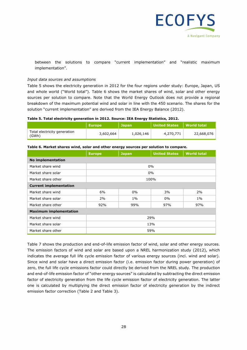
28
between the solutions to compare “current implementation” and “realistic maximum
implementation”.
Input data sources and assumptions
Table 5 shows the electricity generation in 2012 for the four regions under study: Europe, Japan, US
and whole world (“World total”). Table 6 shows the market shares of wind, solar and other energy
sources per solution to compare. Note that the World Energy Outlook does not provide a regional
breakdown of the maximum potential wind and solar in line with the 450 scenario. The shares for the
solution “current implementation” are derived from the IEA Energy Balance (2012).
Table 5. Total electricity generation in 2012. Source: IEA Energy Statistics, 2012.
Europe Japan United States World total
Total electricity generation (GWh)
3,602,664 1,026,146 4,270,771 22,668,076
Table 6. Market shares wind, solar and other energy sources per solution to compare.
Europe Japan United States World total
No implementation
Market share wind 0%
Market share solar 0%
Market share other 100%
Current implementation
Market share wind 6% 0% 3% 2%
Market share solar 2% 1% 0% 1%
Market share other 92% 99% 97% 97%
Maximum implementation
Market share wind 29%
Market share solar 13%
Market share other 59%
Table 7 shows the production and end-of-life emission factor of wind, solar and other energy sources.
The emission factors of wind and solar are based upon a NREL harmonization study (2012), which
indicates the average full life cycle emission factor of various energy sources (incl. wind and solar).
Since wind and solar have a direct emission factor (i.e. emission factor during power generation) of
zero, the full life cycle emissions factor could directly be derived from the NREL study. The production
and end-of-life emission factor of “other energy sources” is calculated by subtracting the direct emission
factor of electricity generation from the life cycle emission factor of electricity generation. The latter
one is calculated by multiplying the direct emission factor of electricity generation by the indirect
emission factor correction (Table 2 and Table 3).
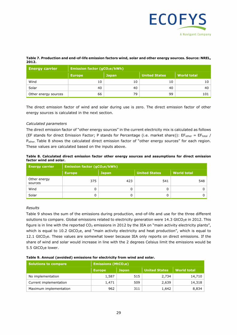
29
Table 7. Production and end-of-life emission factors wind, solar and other energy sources. Source: NREL, 2012.
Energy carrier Emission factor (gCO2e/kWh)
Europe Japan United States World total
Wind 10 10 10 10
Solar 40 40 40 40
Other energy sources 66 79 99 101
The direct emission factor of wind and solar during use is zero. The direct emission factor of other
energy sources is calculated in the next section.
Calculated parameters
The direct emission factor of “other energy sources” in the current electricity mix is calculated as follows
(EF stands for direct Emission Factor; P stands for Percentage (i.e. market share)): EFother = EFtotal /
Pother. Table 8 shows the calculated direct emission factor of “other energy sources” for each region.
These values are calculated based on the inputs above.
Table 8. Calculated direct emission factor other energy sources and assumptions for direct emission factor wind and solar.
Energy carrier Emission factor (gCO2e/kWh)
Europe Japan United States World total
Other energy sources
375 423 541 548
Wind 0 0 0 0
Solar 0 0 0 0
Results
Table 9 shows the sum of the emissions during production, end-of-life and use for the three different
solutions to compare. Global emissions related to electricity generation were 14.3 GtCO2e in 2012. This
figure is in line with the reported CO2 emissions in 2012 by the IEA on “main activity electricity plants”,
which is equal to 10.2 GtCO2e, and “main activity electricity and heat production”, which is equal to
12.1 GtCO2e. These values are somewhat lower because IEA only reports on direct emissions. If the
share of wind and solar would increase in line with the 2 degrees Celsius limit the emissions would be
5.5 GtCO2e lower.
Table 9. Annual (avoided) emissions for electricity from wind and solar.
Solutions to compare Emissions (MtCO2e)
Europe Japan United States World total
No implementation 1,587 515 2,734 14,710
Current implementation 1,471 509 2,639 14,318
Maximum implementation 962 311 1,642 8,834
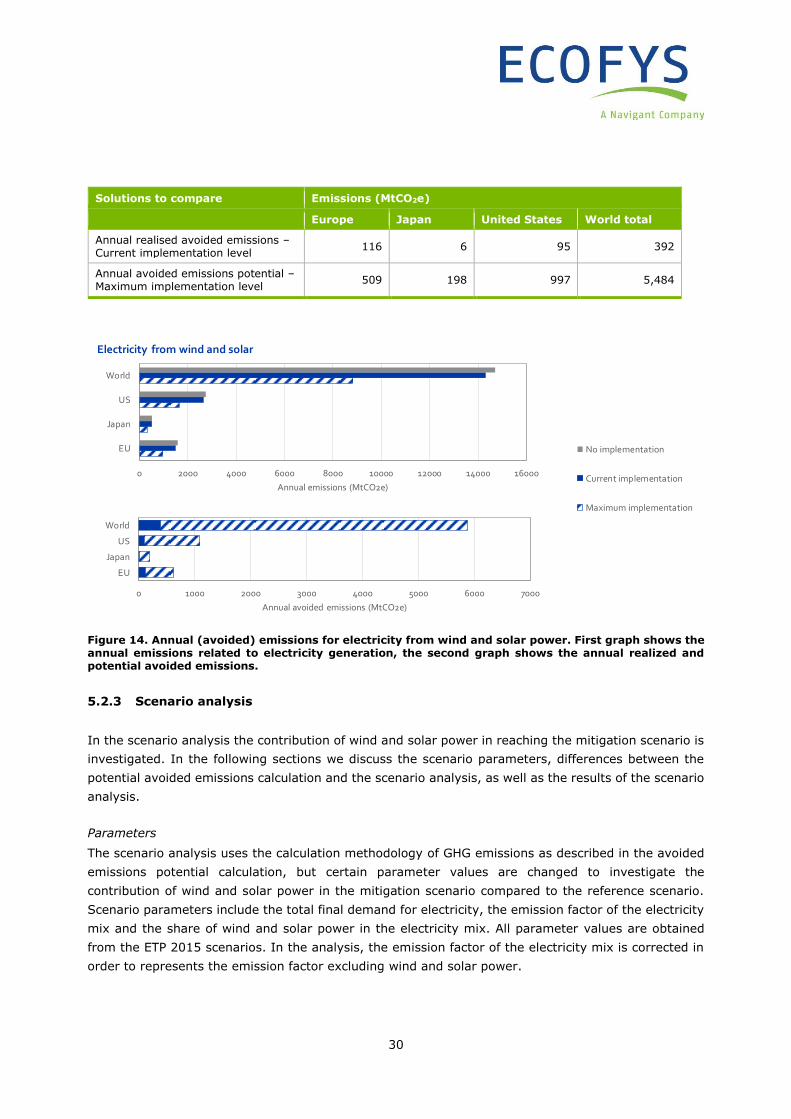
30
Solutions to compare Emissions (MtCO2e)
Europe Japan United States World total
Annual realised avoided emissions – Current implementation level
116 6 95 392
Annual avoided emissions potential – Maximum implementation level
509 198 997 5,484
Figure 14. Annual (avoided) emissions for electricity from wind and solar power. First graph shows the annual emissions related to electricity generation, the second graph shows the annual realized and potential avoided emissions.
5.2.3 Scenario analysis
In the scenario analysis the contribution of wind and solar power in reaching the mitigation scenario is
investigated. In the following sections we discuss the scenario parameters, differences between the
potential avoided emissions calculation and the scenario analysis, as well as the results of the scenario
analysis.
Parameters
The scenario analysis uses the calculation methodology of GHG emissions as described in the avoided
emissions potential calculation, but certain parameter values are changed to investigate the
contribution of wind and solar power in the mitigation scenario compared to the reference scenario.
Scenario parameters include the total final demand for electricity, the emission factor of the electricity
mix and the share of wind and solar power in the electricity mix. All parameter values are obtained
from the ETP 2015 scenarios. In the analysis, the emission factor of the electricity mix is corrected in
order to represents the emission factor excluding wind and solar power.
0 2000 4000 6000 8000 10000 12000 14000 16000
EU
Japan
US
World
Annual emissions (MtCO2e)
Electricity from wind and solar
No implementation
Current implementation
Maximum implementation
0 1000 2000 3000 4000 5000 6000 7000
EU
Japan
US
World
Annual avoided emissions (MtCO2e)
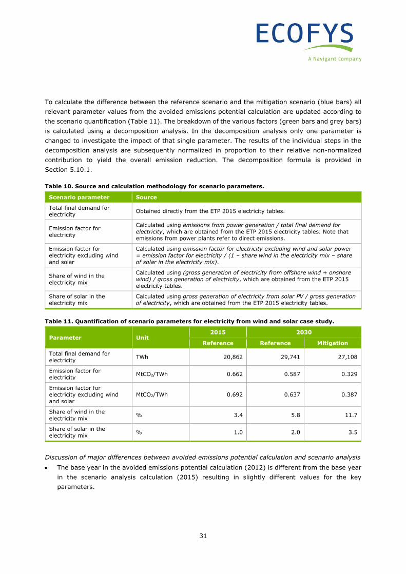
31
To calculate the difference between the reference scenario and the mitigation scenario (blue bars) all
relevant parameter values from the avoided emissions potential calculation are updated according to
the scenario quantification (Table 11). The breakdown of the various factors (green bars and grey bars)
is calculated using a decomposition analysis. In the decomposition analysis only one parameter is
changed to investigate the impact of that single parameter. The results of the individual steps in the
decomposition analysis are subsequently normalized in proportion to their relative non-normalized
contribution to yield the overall emission reduction. The decomposition formula is provided in
Section 5.10.1.
Table 10. Source and calculation methodology for scenario parameters.
Scenario parameter Source
Total final demand for electricity
Obtained directly from the ETP 2015 electricity tables.
Emission factor for electricity
Calculated using emissions from power generation / total final demand for electricity, which are obtained from the ETP 2015 electricity tables. Note that emissions from power plants refer to direct emissions.
Emission factor for electricity excluding wind and solar
Calculated using emission factor for electricity excluding wind and solar power = emission factor for electricity / (1 – share wind in the electricity mix – share of solar in the electricity mix).
Share of wind in the electricity mix
Calculated using (gross generation of electricity from offshore wind + onshore wind) / gross generation of electricity, which are obtained from the ETP 2015 electricity tables.
Share of solar in the electricity mix
Calculated using gross generation of electricity from solar PV / gross generation of electricity, which are obtained from the ETP 2015 electricity tables.
Table 11. Quantification of scenario parameters for electricity from wind and solar case study.
Parameter Unit 2015 2030
Reference Reference Mitigation
Total final demand for electricity
TWh 20,862 29,741 27,108
Emission factor for electricity
MtCO2/TWh 0.662 0.587 0.329
Emission factor for electricity excluding wind and solar
MtCO2/TWh 0.692 0.637 0.387
Share of wind in the electricity mix
% 3.4 5.8 11.7
Share of solar in the electricity mix
% 1.0 2.0 3.5
Discussion of major differences between avoided emissions potential calculation and scenario analysis
• The base year in the avoided emissions potential calculation (2012) is different from the base year
in the scenario analysis calculation (2015) resulting in slightly different values for the key
parameters.
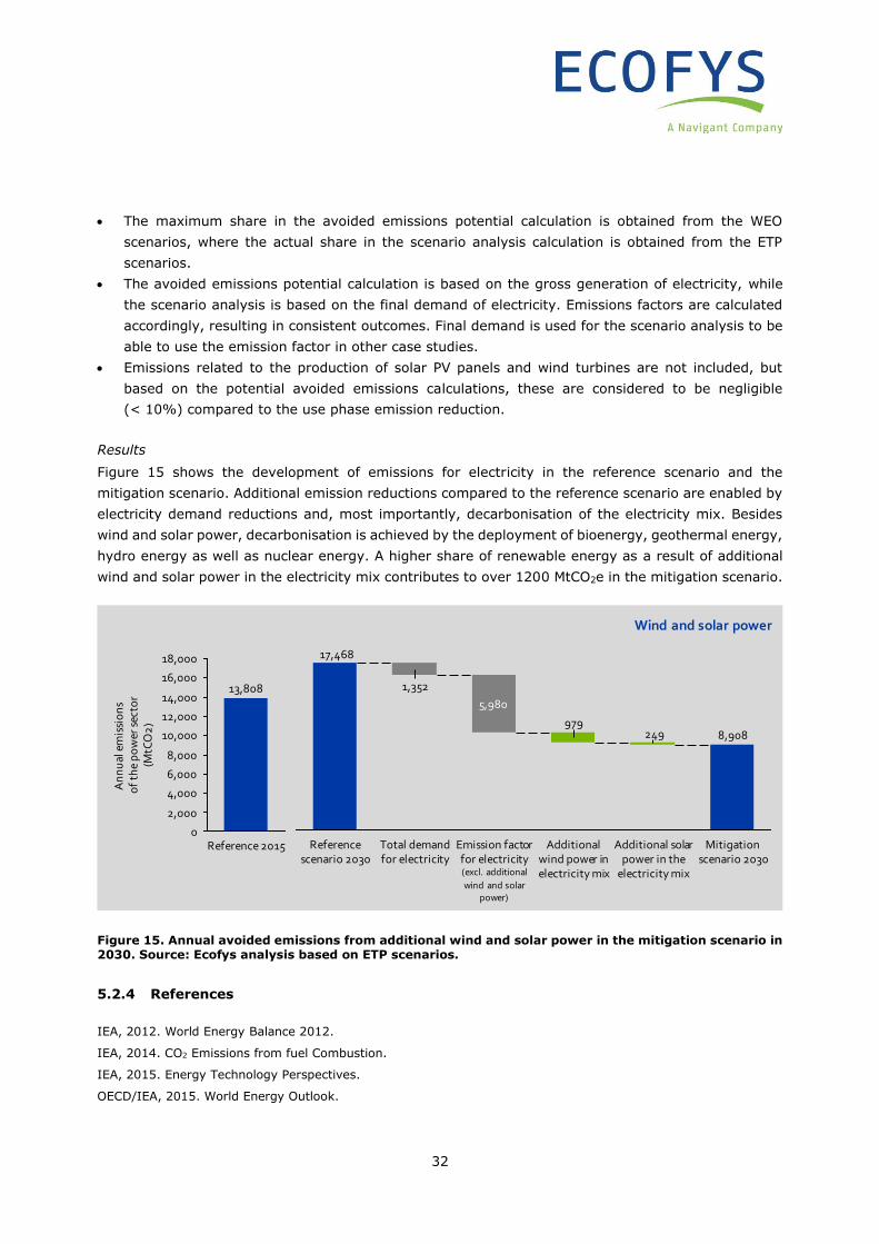
32
• The maximum share in the avoided emissions potential calculation is obtained from the WEO
scenarios, where the actual share in the scenario analysis calculation is obtained from the ETP
scenarios.
• The avoided emissions potential calculation is based on the gross generation of electricity, while
the scenario analysis is based on the final demand of electricity. Emissions factors are calculated
accordingly, resulting in consistent outcomes. Final demand is used for the scenario analysis to be
able to use the emission factor in other case studies.
• Emissions related to the production of solar PV panels and wind turbines are not included, but
based on the potential avoided emissions calculations, these are considered to be negligible
(< 10%) compared to the use phase emission reduction.
Results
Figure 15 shows the development of emissions for electricity in the reference scenario and the
mitigation scenario. Additional emission reductions compared to the reference scenario are enabled by
electricity demand reductions and, most importantly, decarbonisation of the electricity mix. Besides
wind and solar power, decarbonisation is achieved by the deployment of bioenergy, geothermal energy,
hydro energy as well as nuclear energy. A higher share of renewable energy as a result of additional
wind and solar power in the electricity mix contributes to over 1200 MtCO2e in the mitigation scenario.
Figure 15. Annual avoided emissions from additional wind and solar power in the mitigation scenario in 2030. Source: Ecofys analysis based on ETP scenarios.
5.2.4 References
IEA, 2012. World Energy Balance 2012.
IEA, 2014. CO2 Emissions from fuel Combustion.
IEA, 2015. Energy Technology Perspectives.
OECD/IEA, 2015. World Energy Outlook.
Wind and solar power
8,908249979
1,352
17,468
5,980
Reference scenario 2030
Mitigation scenario 2030
Additional solar power in the
electricity mix
Additional wind power in electricity mix
Emission factor for electricity (excl. additional
wind and solar power)
Total demand for electricity
16,000
14,000
12,000
18,000
10,000
8,000
6,000
4,000
2,000
0
An
nu
al e
mis
sio
ns
of
the
po
wer
sec
tor
(MtC
O2
)
Reference 2015
13,808
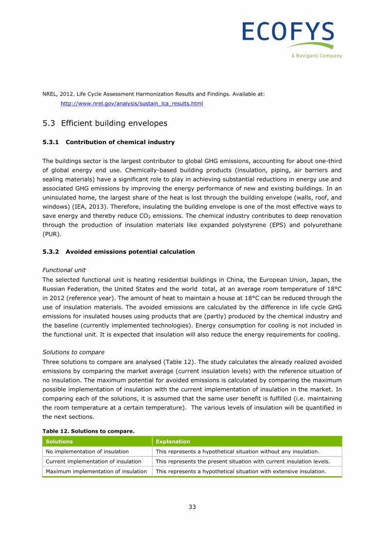
33
NREL, 2012. Life Cycle Assessment Harmonization Results and Findings. Available at:
http://www.nrel.gov/analysis/sustain_lca_results.html
5.3 Efficient building envelopes
5.3.1 Contribution of chemical industry
The buildings sector is the largest contributor to global GHG emissions, accounting for about one-third
of global energy end use. Chemically-based building products (insulation, piping, air barriers and
sealing materials) have a significant role to play in achieving substantial reductions in energy use and
associated GHG emissions by improving the energy performance of new and existing buildings. In an
uninsulated home, the largest share of the heat is lost through the building envelope (walls, roof, and
windows) (IEA, 2013). Therefore, insulating the building envelope is one of the most effective ways to
save energy and thereby reduce CO2 emissions. The chemical industry contributes to deep renovation
through the production of insulation materials like expanded polystyrene (EPS) and polyurethane
(PUR).
5.3.2 Avoided emissions potential calculation
Functional unit
The selected functional unit is heating residential buildings in China, the European Union, Japan, the
Russian Federation, the United States and the world total, at an average room temperature of 18°C
in 2012 (reference year). The amount of heat to maintain a house at 18°C can be reduced through the
use of insulation materials. The avoided emissions are calculated by the difference in life cycle GHG
emissions for insulated houses using products that are (partly) produced by the chemical industry and
the baseline (currently implemented technologies). Energy consumption for cooling is not included in
the functional unit. It is expected that insulation will also reduce the energy requirements for cooling.
Solutions to compare
Three solutions to compare are analysed (Table 12). The study calculates the already realized avoided
emissions by comparing the market average (current insulation levels) with the reference situation of
no insulation. The maximum potential for avoided emissions is calculated by comparing the maximum
possible implementation of insulation with the current implementation of insulation in the market. In
comparing each of the solutions, it is assumed that the same user benefit is fulfilled (i.e. maintaining
the room temperature at a certain temperature). The various levels of insulation will be quantified in
the next sections.
Table 12. Solutions to compare.
Solutions Explanation
No implementation of insulation This represents a hypothetical situation without any insulation.
Current implementation of insulation This represents the present situation with current insulation levels.
Maximum implementation of insulation This represents a hypothetical situation with extensive insulation.
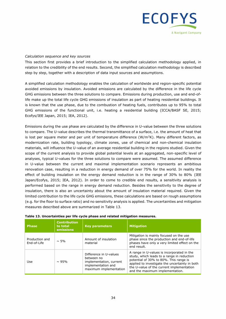
34
Calculation sequence and key sources
This section first provides a brief introduction to the simplified calculation methodology applied, in
relation to the credibility of the end results. Second, the simplified calculation methodology is described
step by step, together with a description of data input sources and assumptions.
A simplified calculation methodology enables the calculation of worldwide and region-specific potential
avoided emissions by insulation. Avoided emissions are calculated by the difference in the life cycle
GHG emissions between the three solutions to compare. Emissions during production, use and end-of-
life make up the total life cycle GHG emissions of insulation as part of heating residential buildings. It
is known that the use phase, due to the combustion of heating fuels, contributes up to 95% to total
GHG emissions of the functional unit, i.e. heating a residential building (ICCA/BASF SE, 2015;
Ecofys/IEE Japan, 2015; IEA, 2012).
Emissions during the use phase are calculated by the difference in U-value between the three solutions
to compare. The U-value describes the thermal transmittance of a surface, i.e. the amount of heat that
is lost per square meter and per unit of temperature difference (W/m2K). Many different factors, as
modernization rate, building typology, climate zones, use of chemical and non-chemical insulation
materials, will influence the U-value of an average residential building in the regions studied. Given the
scope of the current analysis to provide global potential levels at an aggregated, non-specific level of
analyses, typical U-values for the three solutions to compare were assumed. The assumed difference
in U-value between the current and maximal implementation scenario represents an ambitious
renovation case, resulting in a reduction in energy demand of over 75% for the world. In reality the
effect of building insulation on the energy demand reduction is in the range of 30% to 80% (IEE
Japan/Ecofys, 2015; IEA, 2012). In order to come to credible end results, a sensitivity analysis is
performed based on the range in energy demand reduction. Besides the sensitivity to the degree of
insulation, there is also an uncertainty about the amount of insulation material required. Given the
limited contribution to the life cycle GHG emissions, these calculations are based on rough assumptions
(e.g. for the floor to surface ratio) and no sensitivity analysis is applied. The uncertainties and mitigation
measures described above are summarized in Table 13.
Table 13. Uncertainties per life cycle phase and related mitigation measures.
Phase Contribution to total emissions
Key parameters Mitigation
Production and End-of-Life
~ 5% Amount of insulation material
Mitigation is mainly focused on the use phase since the production and end-of-life phases have only a very limited effect on the end result.
Use ~ 95%
Difference in U-values between no implementation, current implementation and maximum implementation
A range in U-values is incorporated in the study, which leads to a range in reduction potential of 30% to 80%. This range is applied to investigate the uncertainty in both the U-value of the current implementation and the maximum implementation.
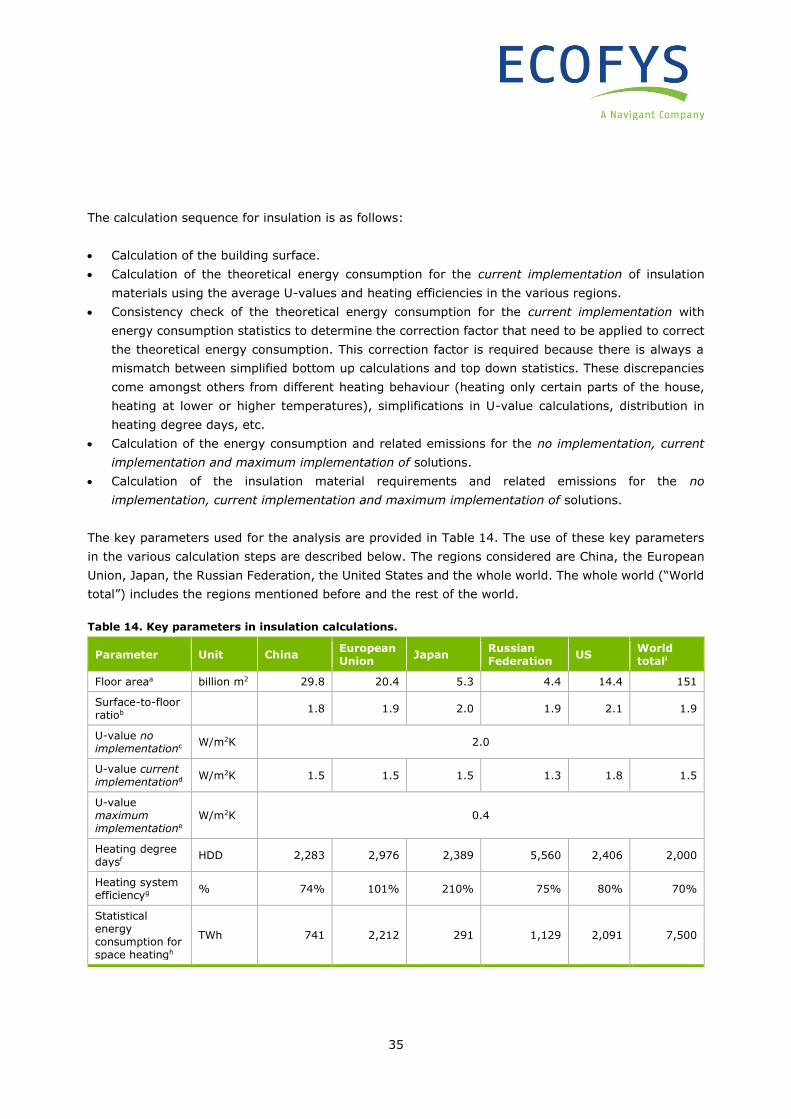
35
The calculation sequence for insulation is as follows:
• Calculation of the building surface.
• Calculation of the theoretical energy consumption for the current implementation of insulation
materials using the average U-values and heating efficiencies in the various regions.
• Consistency check of the theoretical energy consumption for the current implementation with
energy consumption statistics to determine the correction factor that need to be applied to correct
the theoretical energy consumption. This correction factor is required because there is always a
mismatch between simplified bottom up calculations and top down statistics. These discrepancies
come amongst others from different heating behaviour (heating only certain parts of the house,
heating at lower or higher temperatures), simplifications in U-value calculations, distribution in
heating degree days, etc.
• Calculation of the energy consumption and related emissions for the no implementation, current
implementation and maximum implementation of solutions.
• Calculation of the insulation material requirements and related emissions for the no
implementation, current implementation and maximum implementation of solutions.
The key parameters used for the analysis are provided in Table 14. The use of these key parameters
in the various calculation steps are described below. The regions considered are China, the European
Union, Japan, the Russian Federation, the United States and the whole world. The whole world (“World
total”) includes the regions mentioned before and the rest of the world.
Table 14. Key parameters in insulation calculations.
Parameter Unit China European Union
Japan Russian Federation
US World totali
Floor areaa billion m2 29.8 20.4 5.3 4.4 14.4 151
Surface-to-floor ratiob
1.8 1.9 2.0 1.9 2.1 1.9
U-value no implementationc
W/m2K 2.0
U-value current implementationd
W/m2K 1.5 1.5 1.5 1.3 1.8 1.5
U-value maximum implementatione
W/m2K 0.4
Heating degree daysf
HDD 2,283 2,976 2,389 5,560 2,406 2,000
Heating system efficiencyg
% 74% 101% 210% 75% 80% 70%
Statistical energy consumption for space heatingh
TWh 741 2,212 291 1,129 2,091 7,500
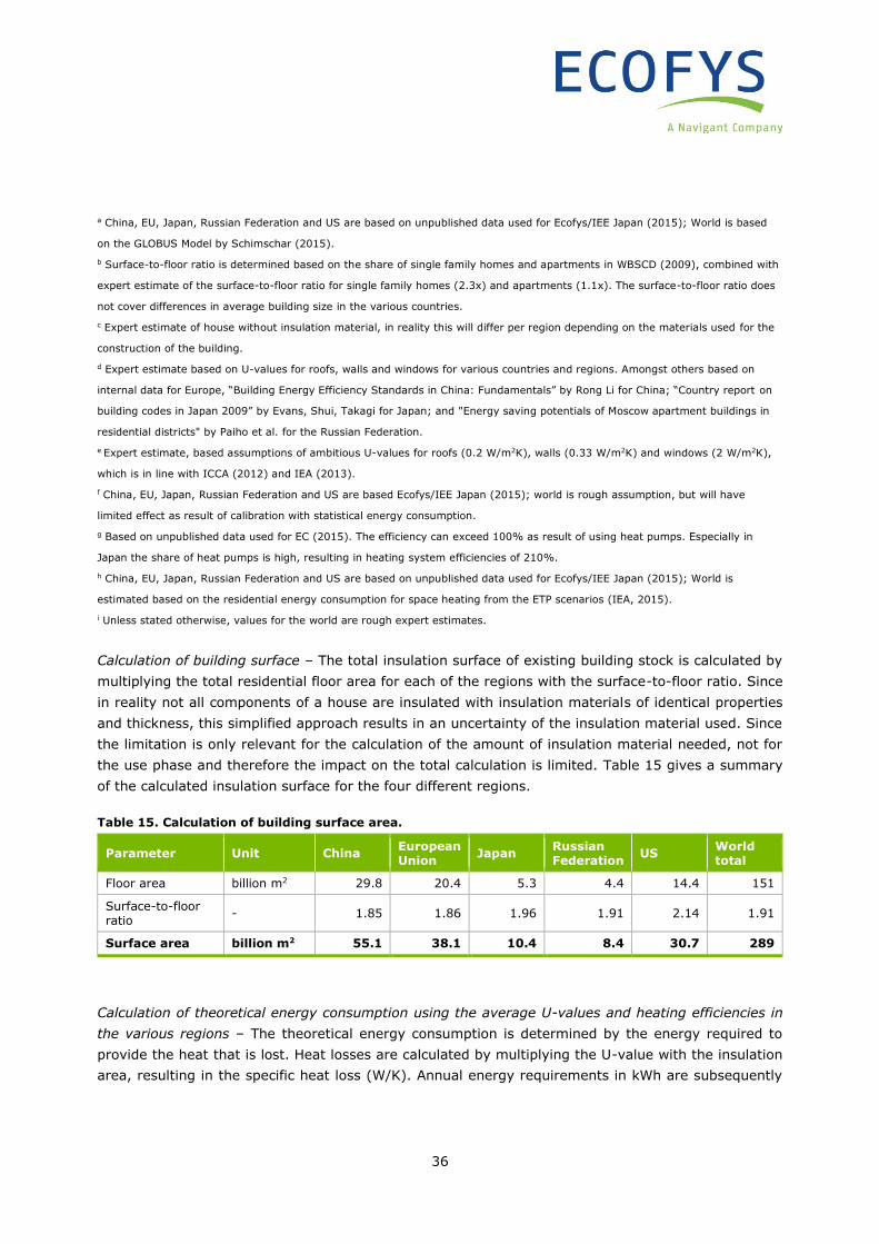
36
a China, EU, Japan, Russian Federation and US are based on unpublished data used for Ecofys/IEE Japan (2015); World is based
on the GLOBUS Model by Schimschar (2015).
b Surface-to-floor ratio is determined based on the share of single family homes and apartments in WBSCD (2009), combined with
expert estimate of the surface-to-floor ratio for single family homes (2.3x) and apartments (1.1x). The surface-to-floor ratio does
not cover differences in average building size in the various countries.
c Expert estimate of house without insulation material, in reality this will differ per region depending on the materials used for the
construction of the building.
d Expert estimate based on U-values for roofs, walls and windows for various countries and regions. Amongst others based on
internal data for Europe, “Building Energy Efficiency Standards in China: Fundamentals” by Rong Li for China; “Country report on
building codes in Japan 2009” by Evans, Shui, Takagi for Japan; and "Energy saving potentials of Moscow apartment buildings in
residential districts" by Paiho et al. for the Russian Federation.
e Expert estimate, based assumptions of ambitious U-values for roofs (0.2 W/m2K), walls (0.33 W/m2K) and windows (2 W/m2K),
which is in line with ICCA (2012) and IEA (2013).
f China, EU, Japan, Russian Federation and US are based Ecofys/IEE Japan (2015); world is rough assumption, but will have
limited effect as result of calibration with statistical energy consumption.
g Based on unpublished data used for EC (2015). The efficiency can exceed 100% as result of using heat pumps. Especially in
Japan the share of heat pumps is high, resulting in heating system efficiencies of 210%.
h China, EU, Japan, Russian Federation and US are based on unpublished data used for Ecofys/IEE Japan (2015); World is
estimated based on the residential energy consumption for space heating from the ETP scenarios (IEA, 2015).
i Unless stated otherwise, values for the world are rough expert estimates.
Calculation of building surface – The total insulation surface of existing building stock is calculated by
multiplying the total residential floor area for each of the regions with the surface-to-floor ratio. Since
in reality not all components of a house are insulated with insulation materials of identical properties
and thickness, this simplified approach results in an uncertainty of the insulation material used. Since
the limitation is only relevant for the calculation of the amount of insulation material needed, not for
the use phase and therefore the impact on the total calculation is limited. Table 15 gives a summary
of the calculated insulation surface for the four different regions.
Table 15. Calculation of building surface area.
Parameter Unit China European Union
Japan Russian Federation
US World total
Floor area billion m2 29.8 20.4 5.3 4.4 14.4 151
Surface-to-floor ratio
- 1.85 1.86 1.96 1.91 2.14 1.91
Surface area billion m2 55.1 38.1 10.4 8.4 30.7 289
Calculation of theoretical energy consumption using the average U-values and heating efficiencies in
the various regions – The theoretical energy consumption is determined by the energy required to
provide the heat that is lost. Heat losses are calculated by multiplying the U-value with the insulation
area, resulting in the specific heat loss (W/K). Annual energy requirements in kWh are subsequently
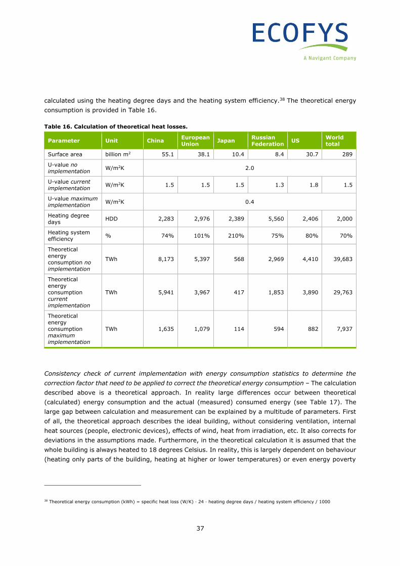
37
calculated using the heating degree days and the heating system efficiency.38 The theoretical energy
consumption is provided in Table 16.
Table 16. Calculation of theoretical heat losses.
Parameter Unit China European Union
Japan Russian Federation
US World total
Surface area billion m2 55.1 38.1 10.4 8.4 30.7 289
U-value no implementation
W/m2K 2.0
U-value current implementation
W/m2K 1.5 1.5 1.5 1.3 1.8 1.5
U-value maximum implementation
W/m2K 0.4
Heating degree days
HDD 2,283 2,976 2,389 5,560 2,406 2,000
Heating system efficiency
% 74% 101% 210% 75% 80% 70%
Theoretical energy consumption no implementation
TWh 8,173 5,397 568 2,969 4,410 39,683
Theoretical energy consumption current implementation
TWh 5,941 3,967 417 1,853 3,890 29,763
Theoretical energy consumption maximum implementation
TWh 1,635 1,079 114 594 882 7,937
Consistency check of current implementation with energy consumption statistics to determine the
correction factor that need to be applied to correct the theoretical energy consumption – The calculation
described above is a theoretical approach. In reality large differences occur between theoretical
(calculated) energy consumption and the actual (measured) consumed energy (see Table 17). The
large gap between calculation and measurement can be explained by a multitude of parameters. First
of all, the theoretical approach describes the ideal building, without considering ventilation, internal
heat sources (people, electronic devices), effects of wind, heat from irradiation, etc. It also corrects for
deviations in the assumptions made. Furthermore, in the theoretical calculation it is assumed that the
whole building is always heated to 18 degrees Celsius. In reality, this is largely dependent on behaviour
(heating only parts of the building, heating at higher or lower temperatures) or even energy poverty
38 Theoretical energy consumption (kWh) = specific heat loss (W/K) ∙ 24 ∙ heating degree days / heating system efficiency / 1000
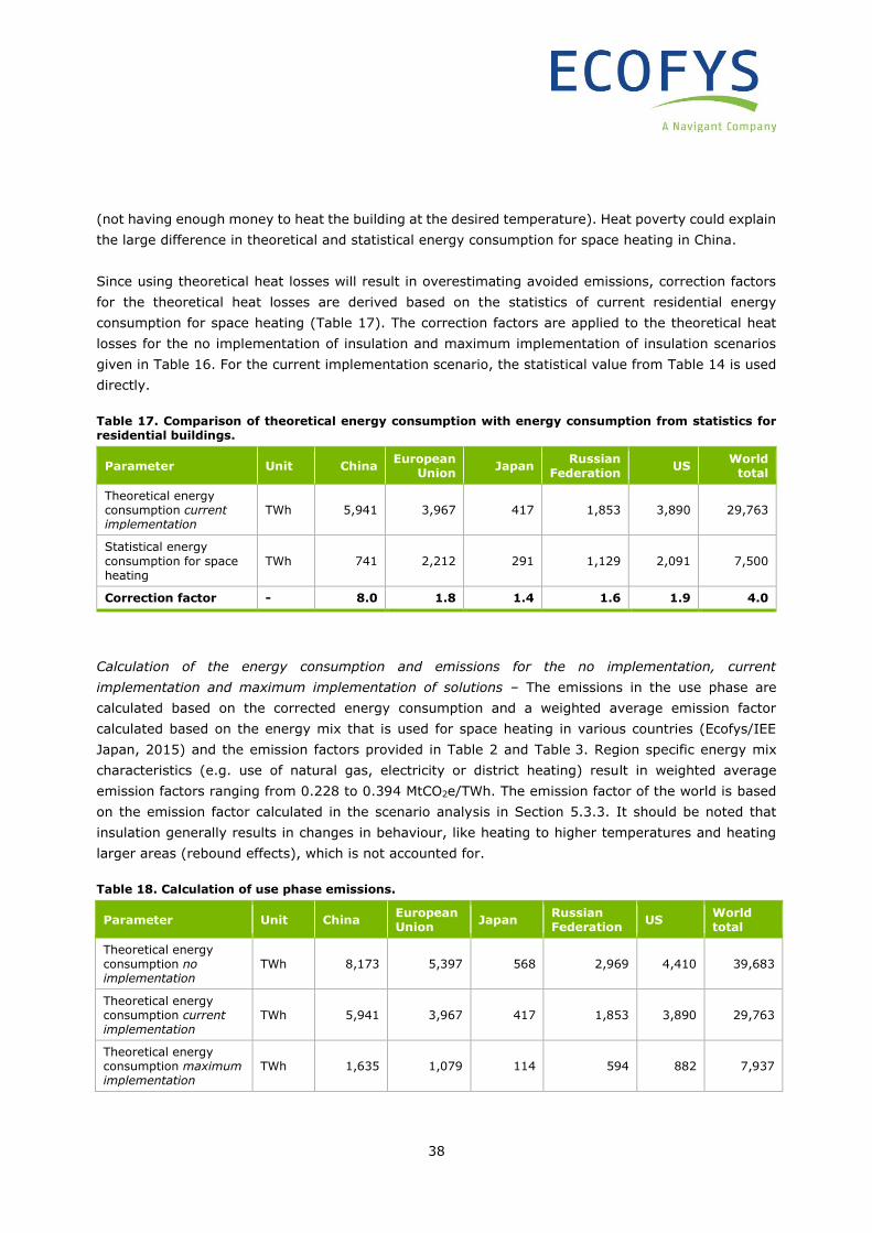
38
(not having enough money to heat the building at the desired temperature). Heat poverty could explain
the large difference in theoretical and statistical energy consumption for space heating in China.
Since using theoretical heat losses will result in overestimating avoided emissions, correction factors
for the theoretical heat losses are derived based on the statistics of current residential energy
consumption for space heating (Table 17). The correction factors are applied to the theoretical heat
losses for the no implementation of insulation and maximum implementation of insulation scenarios
given in Table 16. For the current implementation scenario, the statistical value from Table 14 is used
directly.
Table 17. Comparison of theoretical energy consumption with energy consumption from statistics for residential buildings.
Parameter Unit China European
Union Japan
Russian Federation
US World
total
Theoretical energy consumption current implementation
TWh 5,941 3,967 417 1,853 3,890 29,763
Statistical energy
consumption for space heating
TWh 741 2,212 291 1,129 2,091 7,500
Correction factor - 8.0 1.8 1.4 1.6 1.9 4.0
Calculation of the energy consumption and emissions for the no implementation, current
implementation and maximum implementation of solutions – The emissions in the use phase are
calculated based on the corrected energy consumption and a weighted average emission factor
calculated based on the energy mix that is used for space heating in various countries (Ecofys/IEE
Japan, 2015) and the emission factors provided in Table 2 and Table 3. Region specific energy mix
characteristics (e.g. use of natural gas, electricity or district heating) result in weighted average
emission factors ranging from 0.228 to 0.394 MtCO2e/TWh. The emission factor of the world is based
on the emission factor calculated in the scenario analysis in Section 5.3.3. It should be noted that
insulation generally results in changes in behaviour, like heating to higher temperatures and heating
larger areas (rebound effects), which is not accounted for.
Table 18. Calculation of use phase emissions.
Parameter Unit China European Union
Japan Russian Federation
US World total
Theoretical energy consumption no implementation
TWh 8,173 5,397 568 2,969 4,410 39,683
Theoretical energy consumption current implementation
TWh 5,941 3,967 417 1,853 3,890 29,763
Theoretical energy consumption maximum implementation
TWh 1,635 1,079 114 594 882 7,937
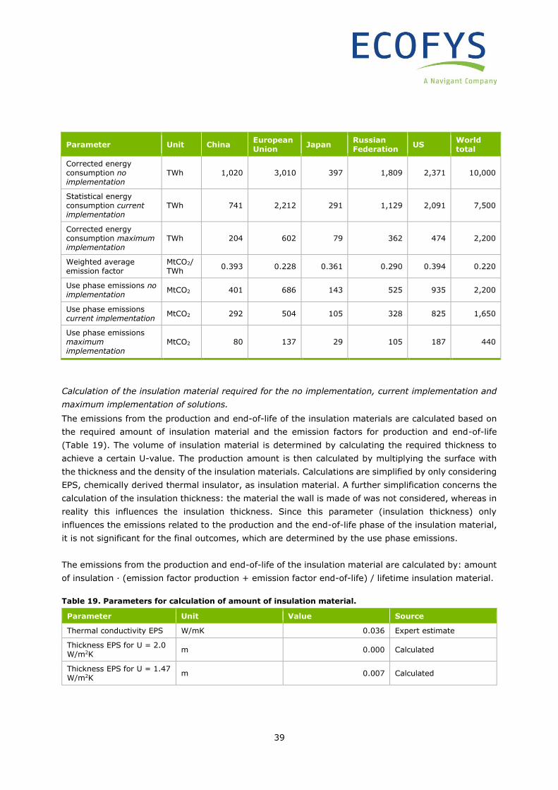
39
Parameter Unit China European Union
Japan Russian Federation
US World total
Corrected energy consumption no implementation
TWh 1,020 3,010 397 1,809 2,371 10,000
Statistical energy consumption current implementation
TWh 741 2,212 291 1,129 2,091 7,500
Corrected energy consumption maximum implementation
TWh 204 602 79 362 474 2,200
Weighted average emission factor
MtCO2/TWh
0.393 0.228 0.361 0.290 0.394 0.220
Use phase emissions no implementation
MtCO2 401 686 143 525 935 2,200
Use phase emissions current implementation
MtCO2 292 504 105 328 825 1,650
Use phase emissions maximum implementation
MtCO2 80 137 29 105 187 440
Calculation of the insulation material required for the no implementation, current implementation and
maximum implementation of solutions.
The emissions from the production and end-of-life of the insulation materials are calculated based on
the required amount of insulation material and the emission factors for production and end-of-life
(Table 19). The volume of insulation material is determined by calculating the required thickness to
achieve a certain U-value. The production amount is then calculated by multiplying the surface with
the thickness and the density of the insulation materials. Calculations are simplified by only considering
EPS, chemically derived thermal insulator, as insulation material. A further simplification concerns the
calculation of the insulation thickness: the material the wall is made of was not considered, whereas in
reality this influences the insulation thickness. Since this parameter (insulation thickness) only
influences the emissions related to the production and the end-of-life phase of the insulation material,
it is not significant for the final outcomes, which are determined by the use phase emissions.
The emissions from the production and end-of-life of the insulation material are calculated by: amount
of insulation ∙ (emission factor production + emission factor end-of-life) / lifetime insulation material.
Table 19. Parameters for calculation of amount of insulation material.
Parameter Unit Value Source
Thermal conductivity EPS W/mK 0.036 Expert estimate
Thickness EPS for U = 2.0 W/m2K
m 0.000 Calculated
Thickness EPS for U = 1.47 W/m2K
m 0.007 Calculated
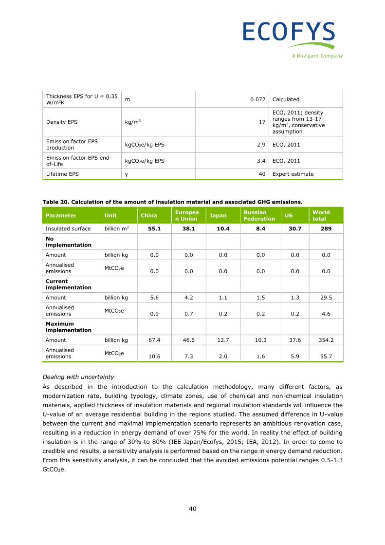
40
Thickness EPS for U = 0.35 W/m2K
m 0.072 Calculated
Density EPS kg/m3 17
ECO, 2011; density ranges from 13-17 kg/m3, conservative assumption
Emission factor EPS production
kgCO2e/kg EPS 2.9 ECO, 2011
Emission factor EPS end-of-Life
kgCO2e/kg EPS 3.4 ECO, 2011
Lifetime EPS y 40 Expert estimate
Table 20. Calculation of the amount of insulation material and associated GHG emissions.
Parameter Unit China European Union
Japan Russian Federation
US World total
Insulated surface billion m2 55.1 38.1 10.4 8.4 30.7 289
No implementation
Amount billion kg 0.0 0.0 0.0 0.0 0.0 0.0
Annualised emissions
MtCO2e 0.0 0.0 0.0 0.0 0.0 0.0
Current implementation
Amount billion kg 5.6 4.2 1.1 1.5 1.3 29.5
Annualised emissions
MtCO2e 0.9 0.7 0.2 0.2 0.2 4.6
Maximum implementation
Amount billion kg 67.4 46.6 12.7 10.3 37.6 354.2
Annualised emissions
MtCO2e 10.6 7.3 2.0 1.6 5.9 55.7
Dealing with uncertainty
As described in the introduction to the calculation methodology, many different factors, as
modernization rate, building typology, climate zones, use of chemical and non-chemical insulation
materials, applied thickness of insulation materials and regional insulation standards will influence the
U-value of an average residential building in the regions studied. The assumed difference in U-value
between the current and maximal implementation scenario represents an ambitious renovation case,
resulting in a reduction in energy demand of over 75% for the world. In reality the effect of building
insulation is in the range of 30% to 80% (IEE Japan/Ecofys, 2015; IEA, 2012). In order to come to
credible end results, a sensitivity analysis is performed based on the range in energy demand reduction.
From this sensitivity analysis, it can be concluded that the avoided emissions potential ranges 0.5-1.3
GtCO2e.
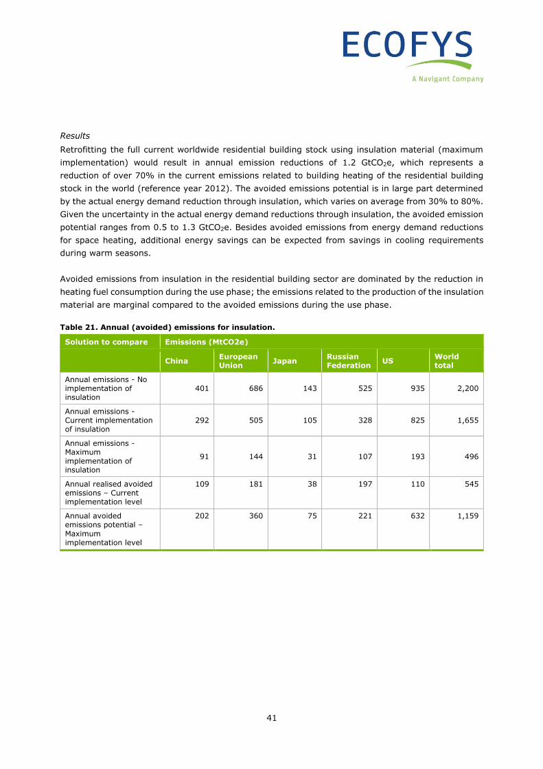
41
Results
Retrofitting the full current worldwide residential building stock using insulation material (maximum
implementation) would result in annual emission reductions of 1.2 GtCO2e, which represents a
reduction of over 70% in the current emissions related to building heating of the residential building
stock in the world (reference year 2012). The avoided emissions potential is in large part determined
by the actual energy demand reduction through insulation, which varies on average from 30% to 80%.
Given the uncertainty in the actual energy demand reductions through insulation, the avoided emission
potential ranges from 0.5 to 1.3 GtCO2e. Besides avoided emissions from energy demand reductions
for space heating, additional energy savings can be expected from savings in cooling requirements
during warm seasons.
Avoided emissions from insulation in the residential building sector are dominated by the reduction in
heating fuel consumption during the use phase; the emissions related to the production of the insulation
material are marginal compared to the avoided emissions during the use phase.
Table 21. Annual (avoided) emissions for insulation.
Solution to compare Emissions (MtCO2e)
China European Union
Japan Russian Federation
US World total
Annual emissions - No implementation of insulation
401 686 143 525 935 2,200
Annual emissions - Current implementation of insulation
292 505 105 328 825 1,655
Annual emissions -Maximum implementation of insulation
91 144 31 107 193 496
Annual realised avoided emissions – Current implementation level
109 181 38 197 110 545
Annual avoided emissions potential –
Maximum implementation level
202 360 75 221 632 1,159
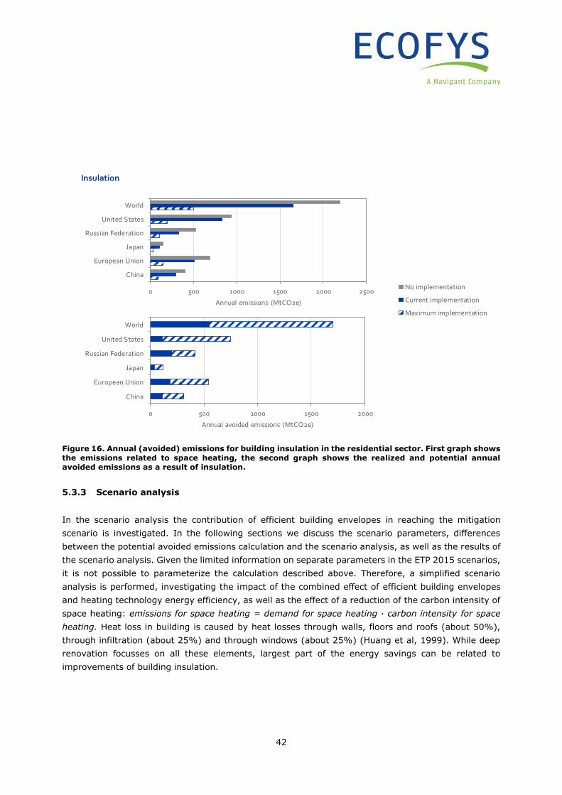
42
Figure 16. Annual (avoided) emissions for building insulation in the residential sector. First graph shows
the emissions related to space heating, the second graph shows the realized and potential annual avoided emissions as a result of insulation.
5.3.3 Scenario analysis
In the scenario analysis the contribution of efficient building envelopes in reaching the mitigation
scenario is investigated. In the following sections we discuss the scenario parameters, differences
between the potential avoided emissions calculation and the scenario analysis, as well as the results of
the scenario analysis. Given the limited information on separate parameters in the ETP 2015 scenarios,
it is not possible to parameterize the calculation described above. Therefore, a simplified scenario
analysis is performed, investigating the impact of the combined effect of efficient building envelopes
and heating technology energy efficiency, as well as the effect of a reduction of the carbon intensity of
space heating: emissions for space heating = demand for space heating · carbon intensity for space
heating. Heat loss in building is caused by heat losses through walls, floors and roofs (about 50%),
through infiltration (about 25%) and through windows (about 25%) (Huang et al, 1999). While deep
renovation focusses on all these elements, largest part of the energy savings can be related to
improvements of building insulation.
0 500 1000 1500 2000 2500
China
European Union
Japan
Russian Federation
United States
World
Annual emissions (MtCO2e)
Insulation
No implementation
Current implementation
Maximum implementation
0 500 1000 1500 2000
China
European Union
Japan
Russian Federation
United States
World
Annual avoided emissions (MtCO2e)
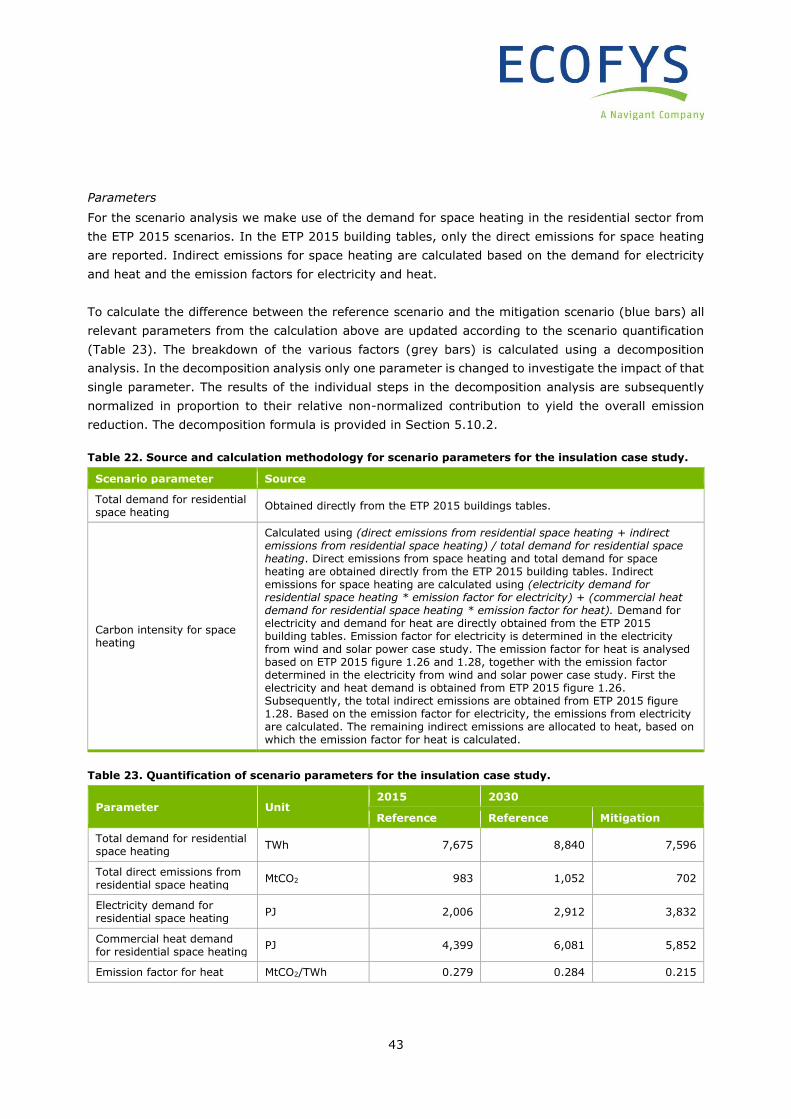
43
Parameters
For the scenario analysis we make use of the demand for space heating in the residential sector from
the ETP 2015 scenarios. In the ETP 2015 building tables, only the direct emissions for space heating
are reported. Indirect emissions for space heating are calculated based on the demand for electricity
and heat and the emission factors for electricity and heat.
To calculate the difference between the reference scenario and the mitigation scenario (blue bars) all
relevant parameters from the calculation above are updated according to the scenario quantification
(Table 23). The breakdown of the various factors (grey bars) is calculated using a decomposition
analysis. In the decomposition analysis only one parameter is changed to investigate the impact of that
single parameter. The results of the individual steps in the decomposition analysis are subsequently
normalized in proportion to their relative non-normalized contribution to yield the overall emission
reduction. The decomposition formula is provided in Section 5.10.2.
Table 22. Source and calculation methodology for scenario parameters for the insulation case study.
Scenario parameter Source
Total demand for residential space heating
Obtained directly from the ETP 2015 buildings tables.
Carbon intensity for space heating
Calculated using (direct emissions from residential space heating + indirect emissions from residential space heating) / total demand for residential space heating. Direct emissions from space heating and total demand for space heating are obtained directly from the ETP 2015 building tables. Indirect emissions for space heating are calculated using (electricity demand for residential space heating * emission factor for electricity) + (commercial heat demand for residential space heating * emission factor for heat). Demand for electricity and demand for heat are directly obtained from the ETP 2015 building tables. Emission factor for electricity is determined in the electricity from wind and solar power case study. The emission factor for heat is analysed based on ETP 2015 figure 1.26 and 1.28, together with the emission factor determined in the electricity from wind and solar power case study. First the electricity and heat demand is obtained from ETP 2015 figure 1.26. Subsequently, the total indirect emissions are obtained from ETP 2015 figure 1.28. Based on the emission factor for electricity, the emissions from electricity are calculated. The remaining indirect emissions are allocated to heat, based on which the emission factor for heat is calculated.
Table 23. Quantification of scenario parameters for the insulation case study.
Parameter Unit 2015 2030
Reference Reference Mitigation
Total demand for residential space heating
TWh 7,675 8,840 7,596
Total direct emissions from residential space heating
MtCO2 983 1,052 702
Electricity demand for residential space heating
PJ 2,006 2,912 3,832
Commercial heat demand for residential space heating
PJ 4,399 6,081 5,852
Emission factor for heat MtCO2/TWh 0.279 0.284 0.215
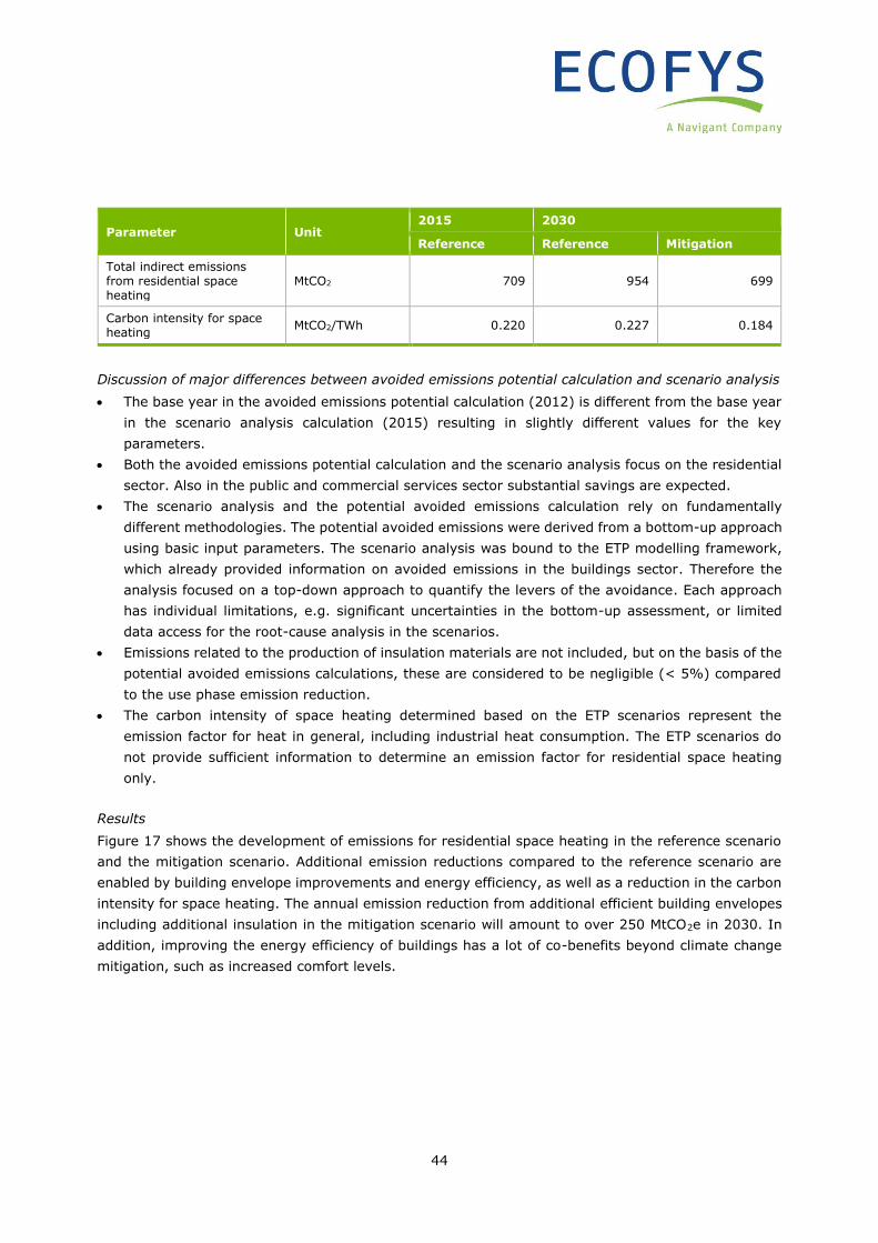
44
Parameter Unit 2015 2030
Reference Reference Mitigation
Total indirect emissions from residential space heating
MtCO2 709 954 699
Carbon intensity for space heating
MtCO2/TWh 0.220 0.227 0.184
Discussion of major differences between avoided emissions potential calculation and scenario analysis
• The base year in the avoided emissions potential calculation (2012) is different from the base year
in the scenario analysis calculation (2015) resulting in slightly different values for the key
parameters.
• Both the avoided emissions potential calculation and the scenario analysis focus on the residential
sector. Also in the public and commercial services sector substantial savings are expected.
• The scenario analysis and the potential avoided emissions calculation rely on fundamentally
different methodologies. The potential avoided emissions were derived from a bottom-up approach
using basic input parameters. The scenario analysis was bound to the ETP modelling framework,
which already provided information on avoided emissions in the buildings sector. Therefore the
analysis focused on a top-down approach to quantify the levers of the avoidance. Each approach
has individual limitations, e.g. significant uncertainties in the bottom-up assessment, or limited
data access for the root-cause analysis in the scenarios.
• Emissions related to the production of insulation materials are not included, but on the basis of the
potential avoided emissions calculations, these are considered to be negligible (< 5%) compared
to the use phase emission reduction.
• The carbon intensity of space heating determined based on the ETP scenarios represent the
emission factor for heat in general, including industrial heat consumption. The ETP scenarios do
not provide sufficient information to determine an emission factor for residential space heating
only.
Results
Figure 17 shows the development of emissions for residential space heating in the reference scenario
and the mitigation scenario. Additional emission reductions compared to the reference scenario are
enabled by building envelope improvements and energy efficiency, as well as a reduction in the carbon
intensity for space heating. The annual emission reduction from additional efficient building envelopes
including additional insulation in the mitigation scenario will amount to over 250 MtCO2e in 2030. In
addition, improving the energy efficiency of buildings has a lot of co-benefits beyond climate change
mitigation, such as increased comfort levels.
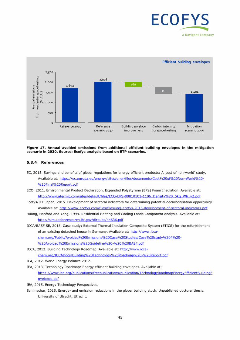
45
Figure 17. Annual avoided emissions from additional efficient building envelopes in the mitigation scenario in 2030. Source: Ecofys analysis based on ETP scenarios.
5.3.4 References
EC, 2015. Savings and benefits of global regulations for energy efficient products: A ‘cost of non-world’ study.
Available at: https://ec.europa.eu/energy/sites/ener/files/documents/Cost%20of%20Non-World%20-
%20Final%20Report.pdf
ECO, 2011. Environmental Product Declaration, Expanded Polystyrene (EPS) Foam Insulation. Available at:
http://www.atermit.com/sites/default/files/ECO-EPS-00010101-1106_Density%20_5kg_Wh_v2.pdf
Ecofys/IEE Japan, 2015. Development of sectoral indicators for determining potential decarbonisation opportunity.
Available at: http://www.ecofys.com/files/files/ieej-ecofys-2015-development-of-sectoral-indicators.pdf
Huang, Hanford and Yang, 1999. Residential Heating and Cooling Loads Component analysis. Available at:
http://simulationresearch.lbl.gov/dirpubs/44636.pdf
ICCA/BASF SE, 2015. Case study: External Thermal Insulation Composite System (ETICS) for the refurbishment
of an existing detached house in Germany. Available at: http://www.icca-
chem.org/Public/Avoided%20Emissions%20Case%20Studies/Case%20study%204%20-
%20Avoided%20Emissions%20Guideline%20-%20%20BASF.pdf
ICCA, 2012. Building Technology Roadmap. Available at: http://www.icca-
chem.org/ICCADocs/Building%20Technology%20Roadmap%20-%20Report.pdf
IEA, 2012. World Energy Balance 2012.
IEA, 2013. Technology Roadmap: Energy efficient building envelopes. Available at:
https://www.iea.org/publications/freepublications/publication/TechnologyRoadmapEnergyEfficientBuildingE
nvelopes.pdf
IEA, 2015. Energy Technology Perspectives.
Schimschar, 2015. Energy- and emission reductions in the global building stock. Unpublished doctoral thesis.
University of Utrecht, Utrecht.
Efficient building envelopes
1,401
2,006
345
260
Mitigation scenario 2030
Carbon intensity for space heating
Building envelope improvement
Reference scenario 2030
0
500
2,500
2,000
1,500
1,000
Reference 2015
1,692
An
nu
al e
mis
sio
ns
fro
m r
esid
enti
al s
pac
e h
eati
ng
(MtC
O2
)
46
WBCSD, 2009. Energy Efficiency in Buildings: Transforming the Market. Available at:
http://www.wbcsd.org/transformingthemarketeeb.aspx
5.4 Efficient lighting
5.4.1 Contribution of chemical industry
Substantial opportunities exist to improve the energy efficiency of appliances in buildings. LED light
bulbs are new and highly energy efficient light bulbs, that have a much higher luminous efficiency than
conventional light bulbs such as incandescent bulbs and halogen bulbs. The energy efficiency potential
of LED light bulbs is up to 80% compared to what is currently applied in the market. Chemical products,
such as semiconductor gas, phosphor, substrates, and sealant, are essential materials to enable high
energy efficiency, reliability, and long life of LED light bulbs.
5.4.2 Avoided emissions potential calculation
Functional unit
The selected functional unit is providing worldwide lighting in the residential and commercial & industry
sector in 2010 (reference year). This functional unit represents 125,934,044 billion lumen hours per
year, of which 21% occurs in the residential sector. The functional unit is calculated based on the
installed stock of lamps in 2010, average wattage and lighting hours from UNEP (2012), complemented
with assumptions on the luminous efficiency and life time per lighting type. Lighting types considered
are incandescent lamps (GLS), tungsten halogen lamps (HAL), compact fluorescent lamps (CFL), light
emitting diodes lamps (LED), high intensity discharge lamps (HID) and linear fluorescent lamps (FL).
The potential avoided emissions are calculated by the difference in life cycle GHG emissions from
lighting with the current mix of lighting types and from lighting with efficient LED only.
Solutions to compare
Four solutions to compare are analysed (Table 24). To determine the realized potential in 2010, the
current implementation is compared to the hypothetical situation of no implementation of LED lighting.
To determine the potential avoided emissions, the maximum implementation of LED lighting is
compared to the current implementation. According to the ICCA & WBCSD guidelines (2013) “solutions
to be compared shall be distributed/used on the market, and not in the process of being banned, in the
reference time period and geographic region.” While incandescent lighting was used on the market in
the reference period, many countries are currently in the process of phasing out (certain types of)
incandescent lighting. Therefore, a fourth solution, representing phasing out of incandescent lighting,
is added to illustrate the potential of LED lighting compared to a situation where incandescent lighting
is phased out. Figure 18 and Figure 19 show the global market shares (based on amount of light
provided) of the six lighting types considered in the four solutions to compare.
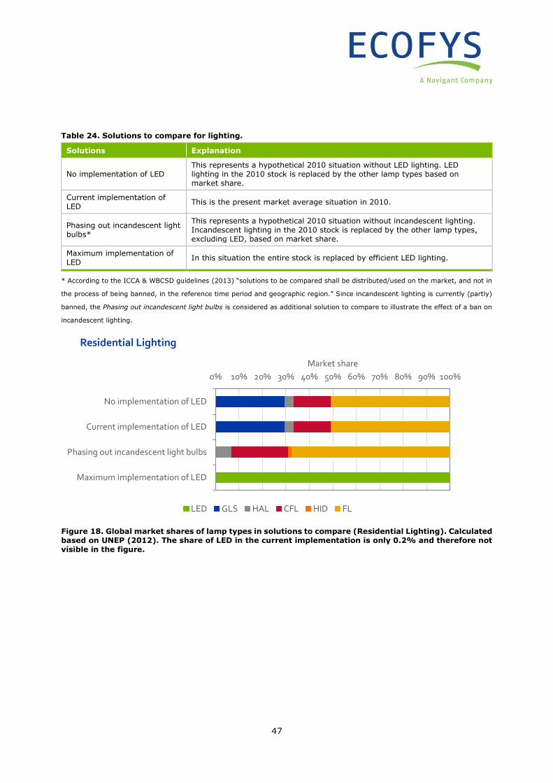
47
Table 24. Solutions to compare for lighting.
Solutions Explanation
No implementation of LED This represents a hypothetical 2010 situation without LED lighting. LED lighting in the 2010 stock is replaced by the other lamp types based on market share.
Current implementation of LED
This is the present market average situation in 2010.
Phasing out incandescent light bulbs*
This represents a hypothetical 2010 situation without incandescent lighting. Incandescent lighting in the 2010 stock is replaced by the other lamp types, excluding LED, based on market share.
Maximum implementation of LED
In this situation the entire stock is replaced by efficient LED lighting.
* According to the ICCA & WBCSD guidelines (2013) “solutions to be compared shall be distributed/used on the market, and not in
the process of being banned, in the reference time period and geographic region.” Since incandescent lighting is currently (partly)
banned, the Phasing out incandescent light bulbs is considered as additional solution to compare to illustrate the effect of a ban on
incandescent lighting.
Figure 18. Global market shares of lamp types in solutions to compare (Residential Lighting). Calculated based on UNEP (2012). The share of LED in the current implementation is only 0.2% and therefore not visible in the figure.
0% 10% 20% 30% 40% 50% 60% 70% 80% 90% 100%
No implementation of LED
Current implementation of LED
Phasing out incandescent light bulbs
Maximum implementation of LED
Market share
Residential Lighting
LED GLS HAL CFL HID FL

48
Figure 19. Global market shares of lamp types in solutions to compare (Commercial & Industrial Lighting). Calculated based on UNEP (2012). The share of LED in the current implementation is only 0.2% and therefore not visible in the figure.
Calculation sequence and key sources
The avoided emissions are calculated by the difference in the life cycle GHG emissions associated with
providing lighting for one year. Total GHG emissions per solution to compare are calculated as follows:
• Production and end-of-life phase:
o Market shares per lighting type are determined per solution to compare.
o The amount of lamps needed to provide the lighting is determined by dividing the total burning
hours per lamp type by the life time of the lamp type.
o The emissions are calculated by multiplying the number of lamps with the emissions factors for
the production and end-of-life phases.
• Use phase:
o Lighting demand per lamp type is calculated by multiplying the market share per lamp type
with the total lighting demand (functional unit).
o The electricity demand per lamp type is calculated by dividing the lighting demand by the
luminous efficiency
o The emission factor of electricity is a combination of a country specific emission factor for the
direct emissions, combined with a general factor to account for the full life cycle.
o The use phase emissions are calculated by multiplying the electricity demand by the country-
specific emission factor
• The realized and potential avoided emissions are determined by the difference in the life cycle GHG
emissions between the solutions to compare.
0% 10% 20% 30% 40% 50% 60% 70% 80% 90% 100%
No implementation of LED
Current implementation of LED
Phasing out incandescent light bulbs
Maximum implementation of LED
Market share
Commercial/Industrial Lighting
LED GLS HAL CFL HID FL
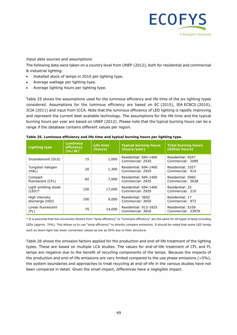
49
Input data sources and assumptions
The following data were taken on a country level from UNEP (2012), both for residential and commercial
& industrial lighting:
• Installed stock of lamps in 2010 per lighting type.
• Average wattage per lighting type.
• Average lighting hours per lighting type.
Table 25 shows the assumptions used for the luminous efficiency and life time of the six lighting types
considered. Assumptions for the luminous efficiency are based on EC (2015), IEA ECBCS (2010),
JCIA (2011) and input from ICCA. Note that the luminous efficiency of LED lighting is rapidly improving
and represent the current best available technology. The assumptions for the life time and the typical
burning hours per year are based on UNEP (2012). Please note that the typical burning hours can be a
range if the database contains different values per region.
Table 25. Luminous efficiency and life time and typical burning hours per lighting type.
Lighting type Luminous efficiency (lm/W)*
Life time (hours)
Typical burning hours (hours/year)
Total burning hours (billion hours)
Incandescent (GLS) 15 1,000 Residential: 694-1460 Commercial: 2920
Residential: 9247 Commercial: 2089
Tungsten halogen (HAL)
20 1,300 Residential: 694-1460 Commercial: 2920
Residential: 1027 Commercial: 914
Compact fluorescent (CFL)
60 7,000 Residential: 694-1460 Commercial: 2920
Residential: 5060 Commercial: 5638
Light emitting diode (LED)*
150 17,000 Residential: 694-1460 Commercial: 2920
Residential: 25 Commercial: 210
High intensity discharge (HID)
100 9,000 Residential: 3650 Commercial: 3650
Residential: 17 Commercial: 972
Linear fluorescent (FL)
75 14,000 Residential: 913-1825 Commercial: 3650
Residential: 5109 Commercial: 23976
* It is assumed that the conversion factors from "lamp efficiency" to "luminaire efficiency" are the same for all types of lamp including
LEDs (approx. 70%). This allows us to use "lamp efficiency" to directly compare emissions. It should be noted that some LED lamps
such as down-light has lower conversion values as low as 50% due to their structure.
Table 26 shows the emission factors applied for the production and end-of-life treatment of the lighting
types. These are based on multiple LCA studies. The values for end-of-life treatment of CFL and FL
lamps are negative due to the benefit of recycling components of the lamps. Because the impacts of
the production and end-of-life emissions are very limited compared to the use phase emissions (<5%),
the system boundaries and approaches to treat recycling at end-of-life in the various studies have not
been compared in detail. Given the small impact, differences have a negligible impact.
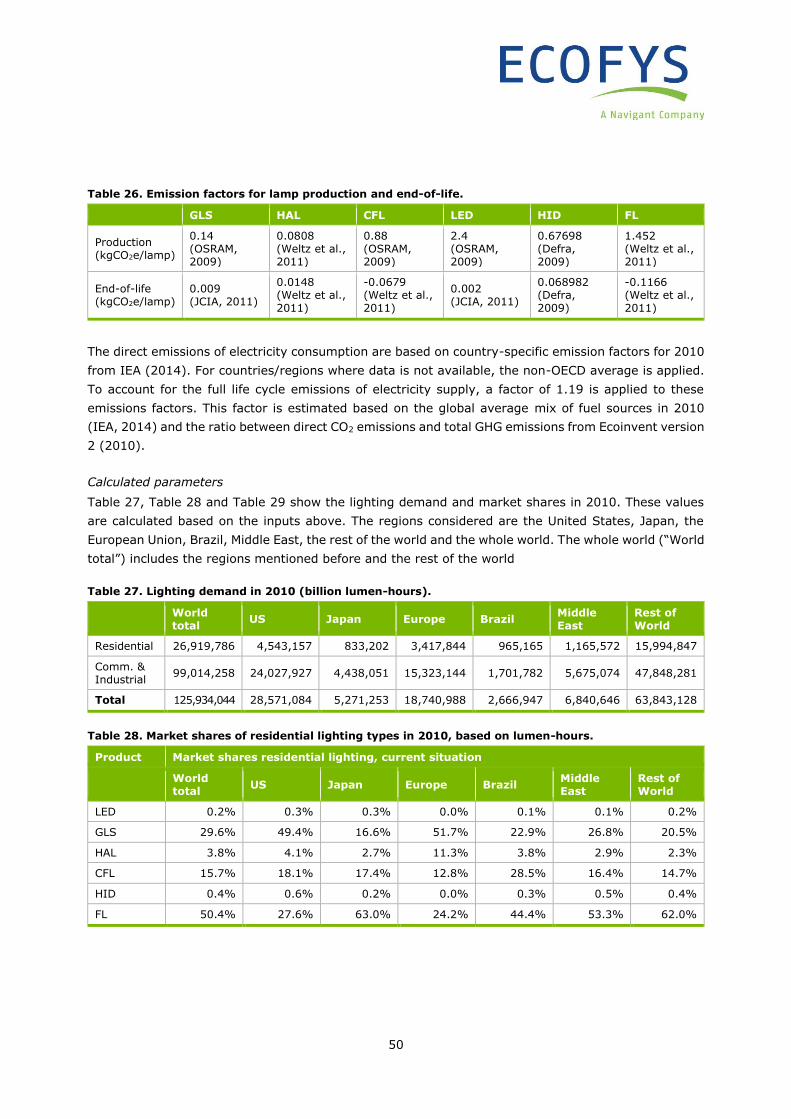
50
Table 26. Emission factors for lamp production and end-of-life.
GLS HAL CFL LED HID FL
Production (kgCO2e/lamp)
0.14 (OSRAM, 2009)
0.0808 (Weltz et al., 2011)
0.88 (OSRAM, 2009)
2.4 (OSRAM, 2009)
0.67698 (Defra, 2009)
1.452 (Weltz et al., 2011)
End-of-life (kgCO2e/lamp)
0.009 (JCIA, 2011)
0.0148 (Weltz et al., 2011)
-0.0679 (Weltz et al., 2011)
0.002 (JCIA, 2011)
0.068982 (Defra, 2009)
-0.1166 (Weltz et al., 2011)
The direct emissions of electricity consumption are based on country-specific emission factors for 2010
from IEA (2014). For countries/regions where data is not available, the non-OECD average is applied.
To account for the full life cycle emissions of electricity supply, a factor of 1.19 is applied to these
emissions factors. This factor is estimated based on the global average mix of fuel sources in 2010
(IEA, 2014) and the ratio between direct CO2 emissions and total GHG emissions from Ecoinvent version
2 (2010).
Calculated parameters
Table 27, Table 28 and Table 29 show the lighting demand and market shares in 2010. These values
are calculated based on the inputs above. The regions considered are the United States, Japan, the
European Union, Brazil, Middle East, the rest of the world and the whole world. The whole world (“World
total”) includes the regions mentioned before and the rest of the world
Table 27. Lighting demand in 2010 (billion lumen-hours).
World total
US Japan Europe Brazil Middle East
Rest of World
Residential 26,919,786 4,543,157 833,202 3,417,844 965,165 1,165,572 15,994,847
Comm. & Industrial
99,014,258 24,027,927 4,438,051 15,323,144 1,701,782 5,675,074 47,848,281
Total 125,934,044 28,571,084 5,271,253 18,740,988 2,666,947 6,840,646 63,843,128
Table 28. Market shares of residential lighting types in 2010, based on lumen-hours.
Product Market shares residential lighting, current situation
World total
US Japan Europe Brazil Middle East
Rest of World
LED 0.2% 0.3% 0.3% 0.0% 0.1% 0.1% 0.2%
GLS 29.6% 49.4% 16.6% 51.7% 22.9% 26.8% 20.5%
HAL 3.8% 4.1% 2.7% 11.3% 3.8% 2.9% 2.3%
CFL 15.7% 18.1% 17.4% 12.8% 28.5% 16.4% 14.7%
HID 0.4% 0.6% 0.2% 0.0% 0.3% 0.5% 0.4%
FL 50.4% 27.6% 63.0% 24.2% 44.4% 53.3% 62.0%
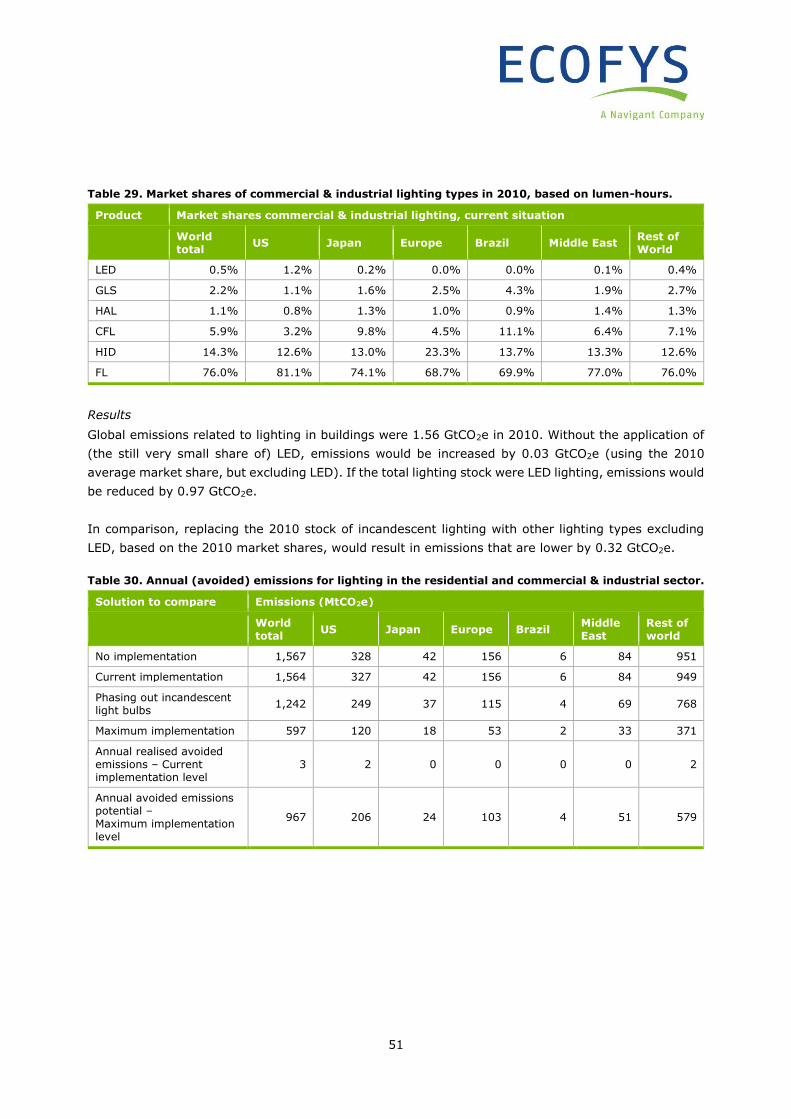
51
Table 29. Market shares of commercial & industrial lighting types in 2010, based on lumen-hours.
Product Market shares commercial & industrial lighting, current situation
World total
US Japan Europe Brazil Middle East Rest of World
LED 0.5% 1.2% 0.2% 0.0% 0.0% 0.1% 0.4%
GLS 2.2% 1.1% 1.6% 2.5% 4.3% 1.9% 2.7%
HAL 1.1% 0.8% 1.3% 1.0% 0.9% 1.4% 1.3%
CFL 5.9% 3.2% 9.8% 4.5% 11.1% 6.4% 7.1%
HID 14.3% 12.6% 13.0% 23.3% 13.7% 13.3% 12.6%
FL 76.0% 81.1% 74.1% 68.7% 69.9% 77.0% 76.0%
Results
Global emissions related to lighting in buildings were 1.56 GtCO2e in 2010. Without the application of
(the still very small share of) LED, emissions would be increased by 0.03 GtCO2e (using the 2010
average market share, but excluding LED). If the total lighting stock were LED lighting, emissions would
be reduced by 0.97 GtCO2e.
In comparison, replacing the 2010 stock of incandescent lighting with other lighting types excluding
LED, based on the 2010 market shares, would result in emissions that are lower by 0.32 GtCO2e.
Table 30. Annual (avoided) emissions for lighting in the residential and commercial & industrial sector.
Solution to compare Emissions (MtCO2e)
World total
US Japan Europe Brazil Middle East
Rest of world
No implementation 1,567 328 42 156 6 84 951
Current implementation 1,564 327 42 156 6 84 949
Phasing out incandescent light bulbs
1,242 249 37 115 4 69 768
Maximum implementation 597 120 18 53 2 33 371
Annual realised avoided emissions – Current implementation level
3 2 0 0 0 0 2
Annual avoided emissions potential – Maximum implementation level
967 206 24 103 4 51 579
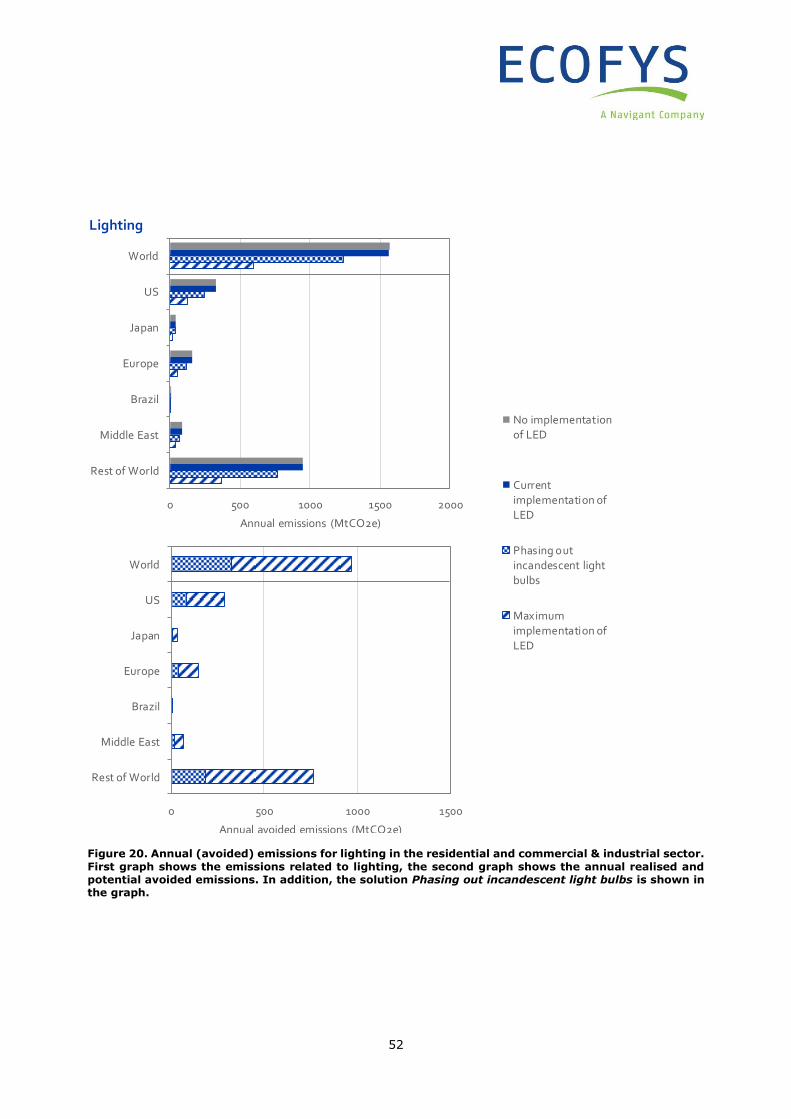
52
Figure 20. Annual (avoided) emissions for lighting in the residential and commercial & industrial sector.
First graph shows the emissions related to lighting, the second graph shows the annual realised and potential avoided emissions. In addition, the solution Phasing out incandescent light bulbs is shown in the graph.
0 500 1000 1500 2000
World
US
Japan
Europe
Brazil
Middle East
Rest of World
Annual emissions (MtCO2e)
Lighting
No implementation
of LED
Current
implementation of
LED
Phasing out
incandescent light
bulbs
Maximum
implementation of
LED
0 500 1000 1500
World
US
Japan
Europe
Brazil
Middle East
Rest of World
Annual avoided emissions (MtCO2e)
53
5.4.3 Scenario analysis
In the scenario analysis, the contribution of LED lighting in reaching the mitigation scenario is
investigated. The following sections discuss the scenario parameters, differences between the potential
avoided emissions calculation and the scenario analysis, as well as the results of the scenario analysis.
The bottom-up data used in the potential avoided emissions calculation result in unrealistic results
when used together with the ETP 2015 data. A slightly simplified approach is therefore applied,
determining the lighting demand based on the electricity demand for lighting together with assumptions
about the current efficiency of lamps.
Parameters
Emissions for lighting are calculated by multiplying electricity demand for lighting by emission factor
for electricity. The electricity demand for lighting is directly obtained from the ETP 2015 building tables
and the emission factor for electricity is calculated in the electricity from wind and solar power case
study.
In addition, further analyses are performed to provide more insights into the role of efficient lighting.
The electricity demand for lighting is split into lighting demand developments and average luminous
efficiency developments: electricity demand for lighting is equal to lighting demand multiplied by
average luminous efficiency. Using the luminous efficiency, the share of LED is determined by solving
the equation 𝜂𝑎𝑣𝑒𝑟𝑎𝑔𝑒 = 𝑥 𝜂𝐿𝐸𝐷 + (1 − 𝑥)𝜂𝑜𝑡ℎ𝑒𝑟 𝑙𝑎𝑚𝑝𝑠 for 𝑥 , where 𝜂𝑎𝑣𝑒𝑟𝑎𝑔𝑒 is average luminous efficiency,
𝜂𝐿𝐸𝐷is luminous efficiency of LED, 𝜂𝑂ℎ𝑡𝑒𝑟 𝑙𝑢𝑚𝑝𝑠is luminous efficiency of other lumps, and 𝑥 is market share
of LED. It is assumed that the efficiency of other lamps is constant over time.
To calculate the difference between the reference scenario and the mitigation scenario (blue bars) all
relevant parameters from the calculation above are updated according to the scenario quantification
(Table 32). The breakdown of the various factors (grey bars) is calculated using a decomposition
analysis. In the decomposition analysis only one parameter is changed to investigate the impact of that
single parameter. The results of the individual steps in the decomposition analysis are subsequently
normalized in proportion to their relative non-normalized contribution to yield the overall emission
reduction. The decomposition formula is provided in Section 5.10.3.
Table 31. Source and calculation methodology for scenario parameters for the lighting case study.
Scenario parameter Source
Electricity demand for lighting
Obtained directly from the ETP 2015 building tables
Emission factor for electricity
Calculated using emissions from power generation / total final demand for electricity, which are obtained from the ETP 2015 electricity tables, as also done in the solar and wind power case study.
Lighting demand The lighting demand in 2015 is calculated by multiplying electricity demand for lighting by average luminous efficiency of lighting. Future years are determined using the increase in floor area, assuming that the lighting demand increases
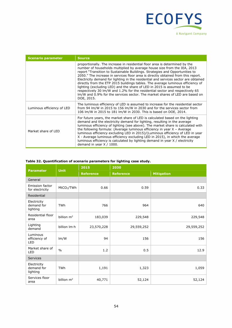
54
Scenario parameter Source
proportionally. The increase in residential floor area is determined by the number of households multiplied by average house size from the IEA, 2013 report “Transition to Sustainable Buildings. Strategies and Opportunities to 2050.” The increase in services floor area is directly obtained from this report. Electricity demand for lighting in the residential and services sector are obtained directly from the ETP 2015 buildings tables. The average luminous efficiency of lighting (excluding LED) and the share of LED in 2015 is assumed to be respectively 30 lm/W and 1.2% for the residential sector and respectively 65 lm/W and 0.9% for the services sector. The market shares of LED are based on DOE, 2015.
Luminous efficiency of LED The luminous efficiency of LED is assumed to increase for the residential sector from 94 lm/W in 2015 to 156 lm/W in 2030 and for the services sector from 106 lm/W in 2015 to 181 lm/W in 2030. This is based on DOE, 2014.
Market share of LED
For future years, the market share of LED is calculated based on the lighting demand and the electricity demand for lighting, resulting in the average luminous efficiency of lighting (see above). The market share is calculated with the following formula: (Average luminous efficiency in year X – Average luminous efficiency excluding LED in 2015)/(Luminous efficiency of LED in year X - Average luminous efficiency excluding LED in 2015), in which the average luminous efficiency is calculated by lighting demand in year X / electricity demand in year X / 1000.
Table 32. Quantification of scenario parameters for lighting case study.
Parameter Unit 2015 2030
Reference Reference Mitigation
General
Emission factor for electricity
MtCO2/TWh 0.66 0.59 0.33
Residential
Electricity demand for lighting
TWh 766 964 640
Residential floor area
billion m2 183,039 229,548 229,548
Lighting demand
billion lm·h 23,570,228 29,559,252 29,559,252
Luminous efficiency of LED
lm/W 94 156 156
Market share of LED
% 1.2 0.5 12.9
Services
Electricity demand for lighting
TWh 1,191 1,323 1,059
Services floor area
billion m2 40,771 52,124 52,124
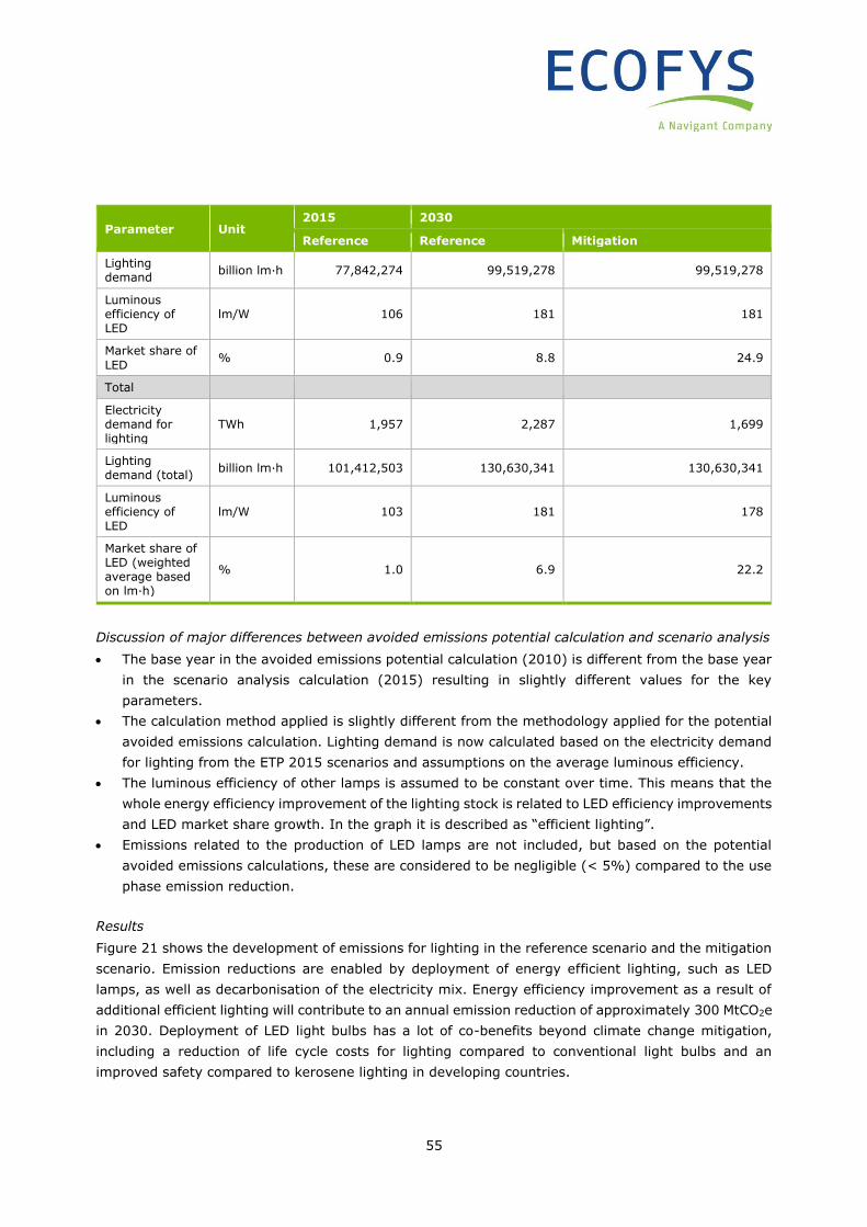
55
Parameter Unit 2015 2030
Reference Reference Mitigation
Lighting demand
billion lm·h 77,842,274 99,519,278 99,519,278
Luminous efficiency of LED
lm/W 106 181 181
Market share of
LED % 0.9 8.8 24.9
Total
Electricity demand for lighting
TWh 1,957 2,287 1,699
Lighting demand (total)
billion lm·h 101,412,503 130,630,341 130,630,341
Luminous efficiency of LED
lm/W 103 181 178
Market share of LED (weighted average based on lm·h)
% 1.0 6.9 22.2
Discussion of major differences between avoided emissions potential calculation and scenario analysis
• The base year in the avoided emissions potential calculation (2010) is different from the base year
in the scenario analysis calculation (2015) resulting in slightly different values for the key
parameters.
• The calculation method applied is slightly different from the methodology applied for the potential
avoided emissions calculation. Lighting demand is now calculated based on the electricity demand
for lighting from the ETP 2015 scenarios and assumptions on the average luminous efficiency.
• The luminous efficiency of other lamps is assumed to be constant over time. This means that the
whole energy efficiency improvement of the lighting stock is related to LED efficiency improvements
and LED market share growth. In the graph it is described as “efficient lighting”.
• Emissions related to the production of LED lamps are not included, but based on the potential
avoided emissions calculations, these are considered to be negligible (< 5%) compared to the use
phase emission reduction.
Results
Figure 21 shows the development of emissions for lighting in the reference scenario and the mitigation
scenario. Emission reductions are enabled by deployment of energy efficient lighting, such as LED
lamps, as well as decarbonisation of the electricity mix. Energy efficiency improvement as a result of
additional efficient lighting will contribute to an annual emission reduction of approximately 300 MtCO2e
in 2030. Deployment of LED light bulbs has a lot of co-benefits beyond climate change mitigation,
including a reduction of life cycle costs for lighting compared to conventional light bulbs and an
improved safety compared to kerosene lighting in developing countries.
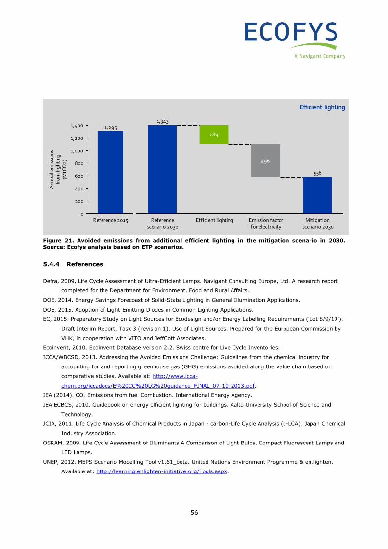
56
Figure 21. Avoided emissions from additional efficient lighting in the mitigation scenario in 2030. Source: Ecofys analysis based on ETP scenarios.
5.4.4 References
Defra, 2009. Life Cycle Assessment of Ultra-Efficient Lamps. Navigant Consulting Europe, Ltd. A research report
completed for the Department for Environment, Food and Rural Affairs.
DOE, 2014. Energy Savings Forecoast of Solid-State Lighting in General Illumination Applications.
DOE, 2015. Adoption of Light-Emitting Diodes in Common Lighting Applications.
EC, 2015. Preparatory Study on Light Sources for Ecodesign and/or Energy Labelling Requirements (‘Lot 8/9/19’).
Draft Interim Report, Task 3 (revision 1). Use of Light Sources. Prepared for the European Commission by
VHK, in cooperation with VITO and JeffCott Associates.
Ecoinvent, 2010. Ecoinvent Database version 2.2. Swiss centre for Live Cycle Inventories.
ICCA/WBCSD, 2013. Addressing the Avoided Emissions Challenge: Guidelines from the chemical industry for
accounting for and reporting greenhouse gas (GHG) emissions avoided along the value chain based on
comparative studies. Available at: http://www.icca-
chem.org/iccadocs/E%20CC%20LG%20guidance_FINAL_07-10-2013.pdf.
IEA (2014). CO2 Emissions from fuel Combustion. International Energy Agency.
IEA ECBCS, 2010. Guidebook on energy efficient lighting for buildings. Aalto University School of Science and
Technology.
JCIA, 2011. Life Cycle Analysis of Chemical Products in Japan - carbon-Life Cycle Analysis (c-LCA). Japan Chemical
Industry Association.
OSRAM, 2009. Life Cycle Assessment of Illuminants A Comparison of Light Bulbs, Compact Fluorescent Lamps and
LED Lamps.
UNEP, 2012. MEPS Scenario Modelling Tool v1.61_beta. United Nations Environment Programme & en.lighten.
Available at: http://learning.enlighten-initiative.org/Tools.aspx.
Efficient lighting
558
1,343
496
289
Reference scenario 2030
Efficient lighting Mitigation scenario 2030
Emission factor for electricity
1,400
1,000
1,200
800
400
200
0
600
An
nu
al e
mis
sio
ns
fro
m li
gh
tin
g(M
tCO
2)
1,295
Reference 2015
57
Welz, Hischier and Hilty, 2011. Environmental impacts of lighting technologies — Life cycle assessment and
sensitivity analysis. In: Environmental Impact Assessment Review, 31, p334-343.
5.5 Transport: Fuel efficient tires
5.5.1 Contribution of chemical industry
Road transport (including cars, busses, and trucks) accounts for more than two thirds of the final
energy consumption.39 Roughly 20% of automobiles' fuel consumption is used to overcome rolling
resistance of the tires (IEA, 2005). Fuel efficient tires have lower rolling resistance compared to normal
tires, while providing enhanced road-gripping performance, resulting in an energy efficiency
improvement of about 2.5% (ICCA/JCIA, 2015). Chemical products such as synthetic rubbers and silica
are key components in reducing energy loss and enabling improved fuel efficiency of tires.
5.5.2 Avoided emissions potential calculation
Functional unit
The selected functional unit is driving passenger cars (“cars”) (12,318 billion kilometres), plus trucks
and buses (“trucks”) (4,241 billion kilometres) in the world in 2010. The potential avoided emissions
are calculated by the difference in life cycle GHG emissions for motor vehicles with fuel efficient tires
and the baseline (currently implemented technologies). Largest part of the difference comes from the
energy savings in the use phase. As stated above, the duration of the function is defined to be one
year, the time reference is set to 2010 and the chosen geographical region is defined to be the world.
Solutions to compare
Three solutions to compare are identified, including no implementation, current implementation, and
maximum implementation of fuel efficient tires. Unfortunately no data is available on global market
shares of fuel efficient tires. The market shares for Japan are used as proxy for the global market
shares for the current implementation (ICCA/JCIA, 2015).
Table 33. Solutions to compare.
Solutions to compare Market shares
Conventional tires Fuel efficient tires
No implementation of fuel efficient tires 100% 0%
Current implementation of fuel efficient tires 81% 19%
Maximum implementation of fuel efficient tires 0% 100%
39 Final energy consumption for road transport for passengers and freight account for 80 EJ compared a total final energy consumption for
transport of 103 EJ in 2012 according to IEA, 2015. Energy Technology Perspectives.
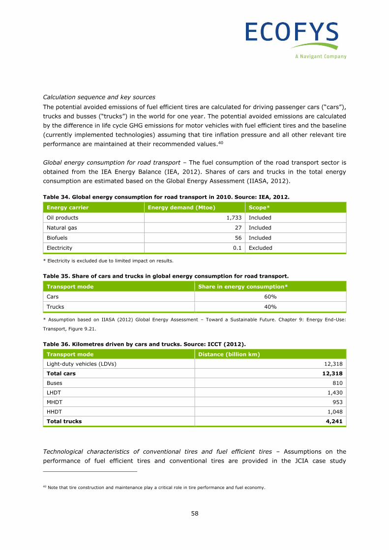
58
Calculation sequence and key sources
The potential avoided emissions of fuel efficient tires are calculated for driving passenger cars (“cars”),
trucks and busses (“trucks”) in the world for one year. The potential avoided emissions are calculated
by the difference in life cycle GHG emissions for motor vehicles with fuel efficient tires and the baseline
(currently implemented technologies) assuming that tire inflation pressure and all other relevant tire
performance are maintained at their recommended values.40
Global energy consumption for road transport – The fuel consumption of the road transport sector is
obtained from the IEA Energy Balance (IEA, 2012). Shares of cars and trucks in the total energy
consumption are estimated based on the Global Energy Assessment (IIASA, 2012).
Table 34. Global energy consumption for road transport in 2010. Source: IEA, 2012.
Energy carrier Energy demand (Mtoe) Scope*
Oil products 1,733 Included
Natural gas 27 Included
Biofuels 56 Included
Electricity 0.1 Excluded
* Electricity is excluded due to limited impact on results.
Table 35. Share of cars and trucks in global energy consumption for road transport.
Transport mode Share in energy consumption*
Cars 60%
Trucks 40%
* Assumption based on IIASA (2012) Global Energy Assessment – Toward a Sustainable Future. Chapter 9: Energy End-Use:
Transport, Figure 9.21.
Table 36. Kilometres driven by cars and trucks. Source: ICCT (2012).
Transport mode Distance (billion km)
Light-duty vehicles (LDVs) 12,318
Total cars 12,318
Buses 810
LHDT 1,430
MHDT 953
HHDT 1,048
Total trucks 4,241
Technological characteristics of conventional tires and fuel efficient tires – Assumptions on the
performance of fuel efficient tires and conventional tires are provided in the JCIA case study
40 Note that tire construction and maintenance play a critical role in tire performance and fuel economy.
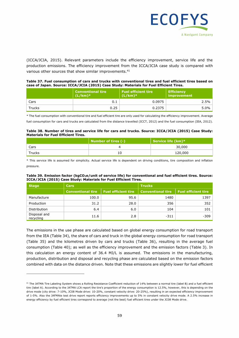
59
(ICCA/JCIA, 2015). Relevant parameters include the efficiency improvement, service life and the
production emissions. The efficiency improvement from the ICCA/JCIA case study is compared with
various other sources that show similar improvements.41
Table 37. Fuel consumption of cars and trucks with conventional tires and fuel efficient tires based on case of Japan. Source: ICCA/JCIA (2015) Case Study: Materials for Fuel Efficient Tires.
Conventional tire (L/km)*
Fuel efficient tire (L/km)*
Efficiency improvement
Cars 0.1 0.0975 2.5%
Trucks 0.25 0.2375 5.0%
* The fuel consumption with conventional tire and fuel efficient tire are only used for calculating the efficiency improvement. Average
fuel consumption for cars and trucks are calculated from the distance travelled (ICCT, 2012) and the fuel consumption (IEA, 2012).
Table 38. Number of tires and service life for cars and trucks. Source: ICCA/JCIA (2015) Case Study: Materials for Fuel Efficient Tires.
Number of tires (-) Service life (km)*
Cars 4 30,000
Trucks 10 120,000
* This service life is assumed for simplicity. Actual service life is dependent on driving conditions, tire composition and inflation
pressure.
Table 39. Emission factor (kgCO2e/unit of service life) for conventional and fuel efficient tires. Source: ICCA/JCIA (2015) Case Study: Materials for Fuel Efficient Tires.
Stage Cars Trucks
Conventional tire Fuel efficient tire Conventional tire Fuel efficient tire
Manufacture 100.0 95.6 1480 1397
Production 31.2 28.0 356 352
Distribution 6.4 6.0 104 101
Disposal and recycling
11.6 2.8 -311 -309
The emissions in the use phase are calculated based on global energy consumption for road transport
from the IEA (Table 34), the share of cars and truck in the global energy consumption for road transport
(Table 35) and the kilometres driven by cars and trucks (Table 36), resulting in the average fuel
consumption (Table 40); as well as the efficiency improvement and the emission factors (Table 3). In
this calculation an energy content of 36.4 MJ/L is assumed. The emissions in the manufacturing,
production, distribution and disposal and recycling phase are calculated based on the emission factors
combined with data on the distance driven. Note that these emissions are slightly lower for fuel efficient
41 The JATMA Tire Labeling System shows a Rolling Resistance Coefficient reduction of 14% between a normal tire (label B) and a fuel efficient
tire (label A). According to the JATMA LCA report the tire’s proportion of the energy consumption is 12.5%, however, this is depending on the
drive mode (city drive: 7-10%, JC08 Mode drive: 10-20%, constant velocity drive: 20-25%), resulting in an expected efficiency improvement
of 1-5%. Also the JAFMAte test drive report reports efficiency improvements up to 5% in constant velocity drive mode. A 2.5% increase in
energy efficiency by fuel efficient tires correspond to average (not the best) fuel efficient tires under the JC08 Mode drive.
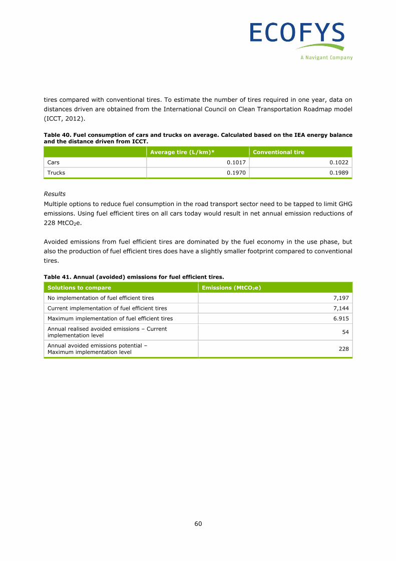
60
tires compared with conventional tires. To estimate the number of tires required in one year, data on
distances driven are obtained from the International Council on Clean Transportation Roadmap model
(ICCT, 2012).
Table 40. Fuel consumption of cars and trucks on average. Calculated based on the IEA energy balance and the distance driven from ICCT.
Average tire (L/km)* Conventional tire
Cars 0.1017 0.1022
Trucks 0.1970 0.1989
Results
Multiple options to reduce fuel consumption in the road transport sector need to be tapped to limit GHG
emissions. Using fuel efficient tires on all cars today would result in net annual emission reductions of
228 MtCO2e.
Avoided emissions from fuel efficient tires are dominated by the fuel economy in the use phase, but
also the production of fuel efficient tires does have a slightly smaller footprint compared to conventional
tires.
Table 41. Annual (avoided) emissions for fuel efficient tires.
Solutions to compare Emissions (MtCO2e)
No implementation of fuel efficient tires 7,197
Current implementation of fuel efficient tires 7,144
Maximum implementation of fuel efficient tires 6.915
Annual realised avoided emissions – Current implementation level
54
Annual avoided emissions potential – Maximum implementation level
228
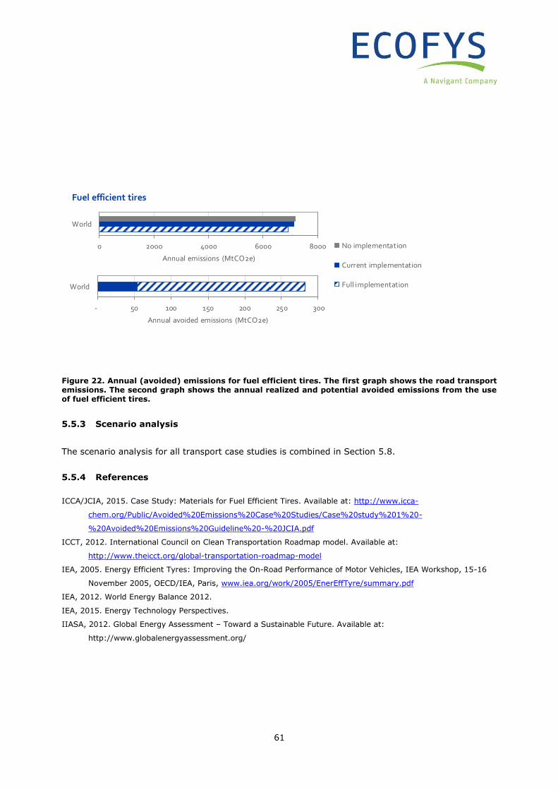
61
Figure 22. Annual (avoided) emissions for fuel efficient tires. The first graph shows the road transport emissions. The second graph shows the annual realized and potential avoided emissions from the use of fuel efficient tires.
5.5.3 Scenario analysis
The scenario analysis for all transport case studies is combined in Section 5.8.
5.5.4 References
ICCA/JCIA, 2015. Case Study: Materials for Fuel Efficient Tires. Available at: http://www.icca-
chem.org/Public/Avoided%20Emissions%20Case%20Studies/Case%20study%201%20-
%20Avoided%20Emissions%20Guideline%20-%20JCIA.pdf
ICCT, 2012. International Council on Clean Transportation Roadmap model. Available at:
http://www.theicct.org/global-transportation-roadmap-model
IEA, 2005. Energy Efficient Tyres: Improving the On-Road Performance of Motor Vehicles, IEA Workshop, 15-16
November 2005, OECD/IEA, Paris, www.iea.org/work/2005/EnerEffTyre/summary.pdf
IEA, 2012. World Energy Balance 2012.
IEA, 2015. Energy Technology Perspectives.
IIASA, 2012. Global Energy Assessment – Toward a Sustainable Future. Available at:
http://www.globalenergyassessment.org/
0 2000 4000 6000 8000
World
Annual emissions (MtCO2e)
Fuel efficient tires
No implementation
Current implementation
Full implementation
- 50 100 150 200 250 300
World
Annual avoided emissions (MtCO2e)
62
5.6 Transport: Lightweight materials for cars
5.6.1 Contribution of chemical industry
Lightweight materials reduce the fuel demand of cars. Innovative lightweight materials reduce car
weight substantially. Chemical products such as plastics and carbon reinforced plastics are key in
achieving strong weight reductions of cars.
5.6.2 Avoided emissions potential calculation
Functional unit
The selected functional unit is driving passenger cars (“cars”) in the world in 2010, which is equal to
12,318 billion kilometres travelled by light duty vehicles for passenger transport (ICCT, 2012). The
potential avoided emissions are calculated by the difference in life cycle GHG emissions for cars with
lightweight materials and the baseline (the current mix of cars with and without lightweight materials).
Different materials are used in car manufacturing: steel, aluminium, high strength steel (HSS), plastics,
magnesium, carbon fibre and other materials. Within this study the scope is limited to lightweight
materials produced by the chemical industry, which are considered to be plastics and carbon fibre
reinforced plastics (further abbreviated as carbon fibre).
Solutions to compare
Three solutions to compare are identified, including no implementation, current implementation and
maximum implementation of lightweight materials (Table 42 and Figure 23). The material mixes of the
current implementation and the maximum implementation are based on the study “Lightweight, heavy
impact: How carbon fibre and other lightweight materials will develop across industries and specifically
in automotive” by McKinsey (2012). The followed methodology will be explained in detail in the next
sections.
Table 42. Three solutions to compare.
Solutions to compare Description
No implementation of lightweight materials
This represents a hypothetical 2010 situation without lightweight materials being used in car manufacturing.
Current implementation of lightweight materials This is the present material mix (incl. lightweight materials) in 2010.
Maximum implementation of lightweight materials This represents a hypothetical situation with a maximum share of lightweight materials in car manufacturing.
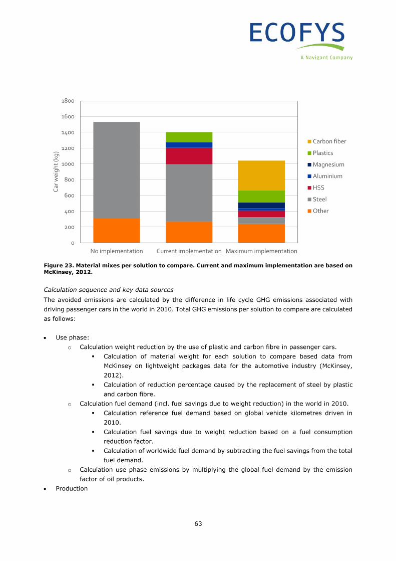
63
Figure 23. Material mixes per solution to compare. Current and maximum implementation are based on McKinsey, 2012.
Calculation sequence and key data sources
The avoided emissions are calculated by the difference in life cycle GHG emissions associated with
driving passenger cars in the world in 2010. Total GHG emissions per solution to compare are calculated
as follows:
• Use phase:
o Calculation weight reduction by the use of plastic and carbon fibre in passenger cars.
▪ Calculation of material weight for each solution to compare based data from
McKinsey on lightweight packages data for the automotive industry (McKinsey,
2012).
▪ Calculation of reduction percentage caused by the replacement of steel by plastic
and carbon fibre.
o Calculation fuel demand (incl. fuel savings due to weight reduction) in the world in 2010.
▪ Calculation reference fuel demand based on global vehicle kilometres driven in
2010.
▪ Calculation fuel savings due to weight reduction based on a fuel consumption
reduction factor.
▪ Calculation of worldwide fuel demand by subtracting the fuel savings from the total
fuel demand.
o Calculation use phase emissions by multiplying the global fuel demand by the emission
factor of oil products.
• Production
0
200
400
600
800
1000
1200
1400
1600
1800
No implementation Current implementation Maximum implementation
Car
wei
gh
t (k
g)
Carbon fiber
Plastics
Magnesium
Aluminium
HSS
Steel
Other
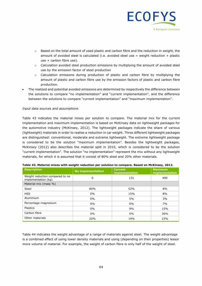
64
o Based on the total amount of used plastic and carbon fibre and the reduction in weight, the
amount of avoided steel is calculated (i.e. avoided steel use = weight reduction + plastic
use + carbon fibre use).
o Calculation avoided steel production emissions by multiplying the amount of avoided steel
use by the emission factor of steel production
o Calculation emissions during production of plastic and carbon fibre by multiplying the
amount of plastic and carbon fibre use by the emission factors of plastic and carbon fibre
production.
• The realized and potential avoided emissions are determined by respectively the difference between
the solutions to compare “no implementation” and “current implementation”, and the difference
between the solutions to compare “current implementation” and “maximum implementation”.
Input data sources and assumptions
Table 43 indicates the material mixes per solution to compare. The material mix for the current
implementation and maximum implementation is based on McKinsey data on lightweight packages for
the automotive industry (McKinsey, 2012). The lightweight packages indicate the share of various
(lightweight) materials in order to realise a reduction in car weight. Three different lightweight packages
are distinguished: conventional, moderate and extreme lightweight. The extreme lightweight package
is considered to be the solution “maximum implementation”. Besides the lightweight packages,
McKinsey (2012) also describes the material split in 2010, which is considered to be the solution
“current implementation”. The solution “no implementation” represent the mix without any lightweight
materials, for which it is assumed that it consist of 80% steel and 20% other materials.
Table 43. Material mixes with weight reduction per solution to compare. Based on McKinsey, 2012.
Description No implementation
Current implementation
Maximum implementation
Weight reduction compared to no implementation (kg)
0 131 490
Material mix (mass %)
Steel 80% 52% 8%
HSS 0% 15% 8%
Aluminium 0% 5% 3%
Percentage magnesium 0% 0% 7%
Plastics 0% 9% 15%
Carbon fibre 0% 0% 36%
Other materials 20% 19% 23%
Table 44 indicates the weight advantage of a range of materials against steel. The weight advantage
is a combined effect of using lower density materials and using (depending on their properties) lessor
more volume of material. For example, the weight of carbon fibre is only half of the weight of steel.
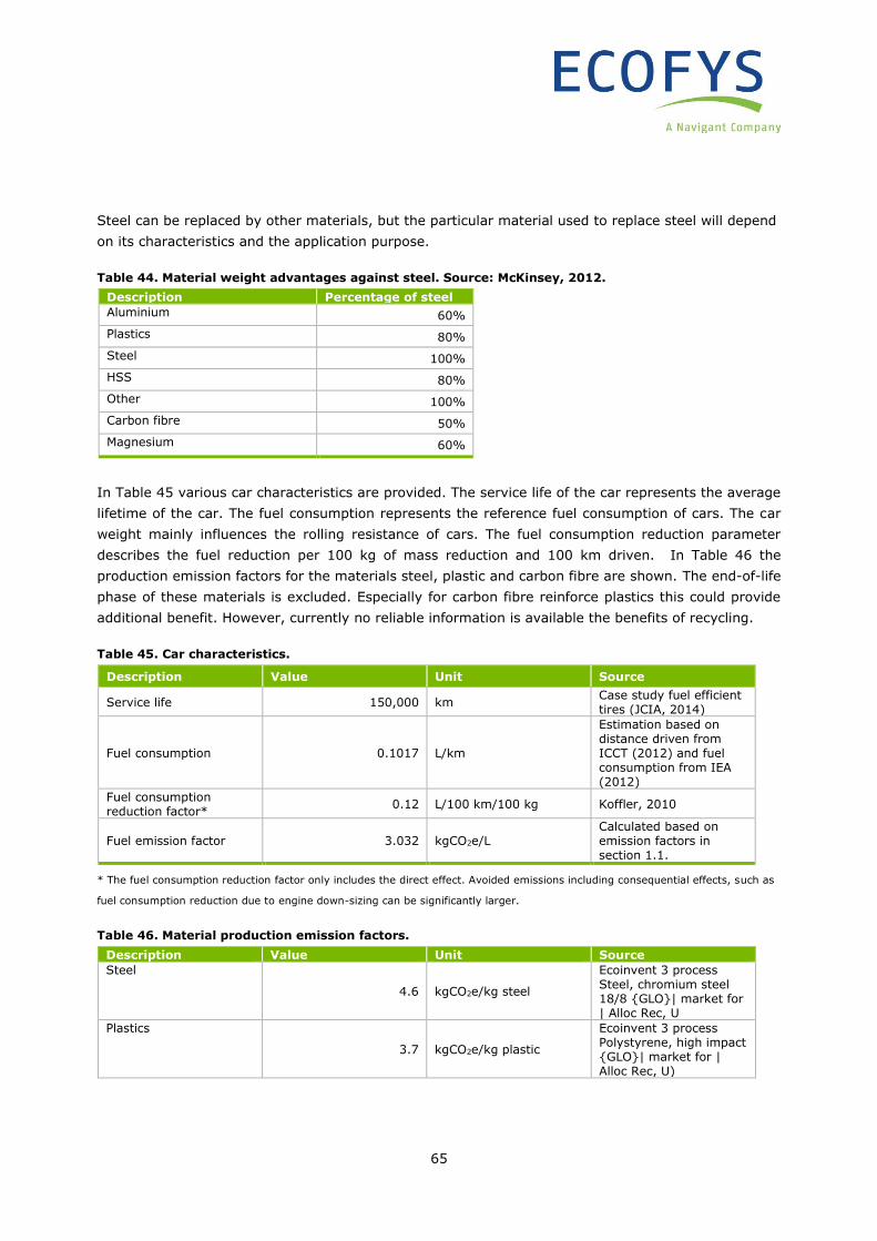
65
Steel can be replaced by other materials, but the particular material used to replace steel will depend
on its characteristics and the application purpose.
Table 44. Material weight advantages against steel. Source: McKinsey, 2012.
Description Percentage of steel
Aluminium 60%
Plastics 80%
Steel 100%
HSS 80%
Other 100%
Carbon fibre 50%
Magnesium 60%
In Table 45 various car characteristics are provided. The service life of the car represents the average
lifetime of the car. The fuel consumption represents the reference fuel consumption of cars. The car
weight mainly influences the rolling resistance of cars. The fuel consumption reduction parameter
describes the fuel reduction per 100 kg of mass reduction and 100 km driven. In Table 46 the
production emission factors for the materials steel, plastic and carbon fibre are shown. The end-of-life
phase of these materials is excluded. Especially for carbon fibre reinforce plastics this could provide
additional benefit. However, currently no reliable information is available the benefits of recycling.
Table 45. Car characteristics.
Description Value Unit Source
Service life 150,000 km Case study fuel efficient tires (JCIA, 2014)
Fuel consumption 0.1017 L/km
Estimation based on distance driven from ICCT (2012) and fuel consumption from IEA (2012)
Fuel consumption reduction factor*
0.12 L/100 km/100 kg Koffler, 2010
Fuel emission factor 3.032 kgCO2e/L Calculated based on emission factors in section 1.1.
* The fuel consumption reduction factor only includes the direct effect. Avoided emissions including consequential effects, such as
fuel consumption reduction due to engine down-sizing can be significantly larger.
Table 46. Material production emission factors.
Description Value Unit Source
Steel
4.6 kgCO2e/kg steel
Ecoinvent 3 process Steel, chromium steel 18/8 {GLO}| market for | Alloc Rec, U
Plastics
3.7 kgCO2e/kg plastic
Ecoinvent 3 process Polystyrene, high impact {GLO}| market for | Alloc Rec, U)
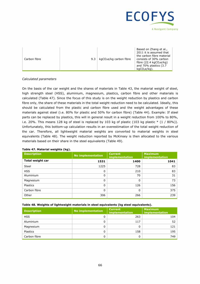
66
Carbon fibre 9.3 kgCO2e/kg carbon fibre
Based on Zhang et al., 2011 it is assumed that the carbon fibre material consists of 30% carbon fibre (22.4 kgCO2e/kg) and 70% plastics (3.7 kgCO2e/kg).
Calculated parameters
On the basis of the car weight and the shares of materials in Table 43, the material weight of steel,
high strength steel (HSS), aluminium, magnesium, plastics, carbon fibre and other materials is
calculated (Table 47). Since the focus of this study is on the weight reduction by plastics and carbon
fibre only, the share of these materials in the total weight reduction need to be calculated. Ideally, this
should be calculated from the plastic and carbon fibre used and the weight advantages of these
materials against steel (i.e. 80% for plastic and 50% for carbon fibre) (Table 44). Example: If steel
parts can be replaced by plastics, this will in general result in a weight reduction from 100% to 80%,
i.e. 20%. This means 128 kg of steel is replaced by 103 kg of plastic (103 kg plastic * (1 / 80%)).
Unfortunately, this bottom-up calculation results in an overestimation of the total weight reduction of
the car. Therefore, all lightweight material weights are converted to material weights in steel
equivalents (Table 48). The weight reduction reported by McKinsey is then allocated to the various
materials based on their share in the steel equivalents (Table 49).
Table 47. Material weights (kg).
Description No implementation
Current implementation
Maximum implementation
Total weight car 1531 1400 1041
Steel 1225 728 83
HSS 0 210 83
Aluminium 0 70 31
Magnesium 0 0 73
Plastics 0 126 156
Carbon fibre 0 0 375
Other 306 266 239
Table 48. Weights of lightweight materials in steel equivalents (kg steel equivalents).
Description No implementation Current implementation
Maximum implementation
HSS 0 263 104
Aluminium 0 117 52
Magnesium 0 0 121
Plastics 0 158 195
Carbon fibre 0 0 749
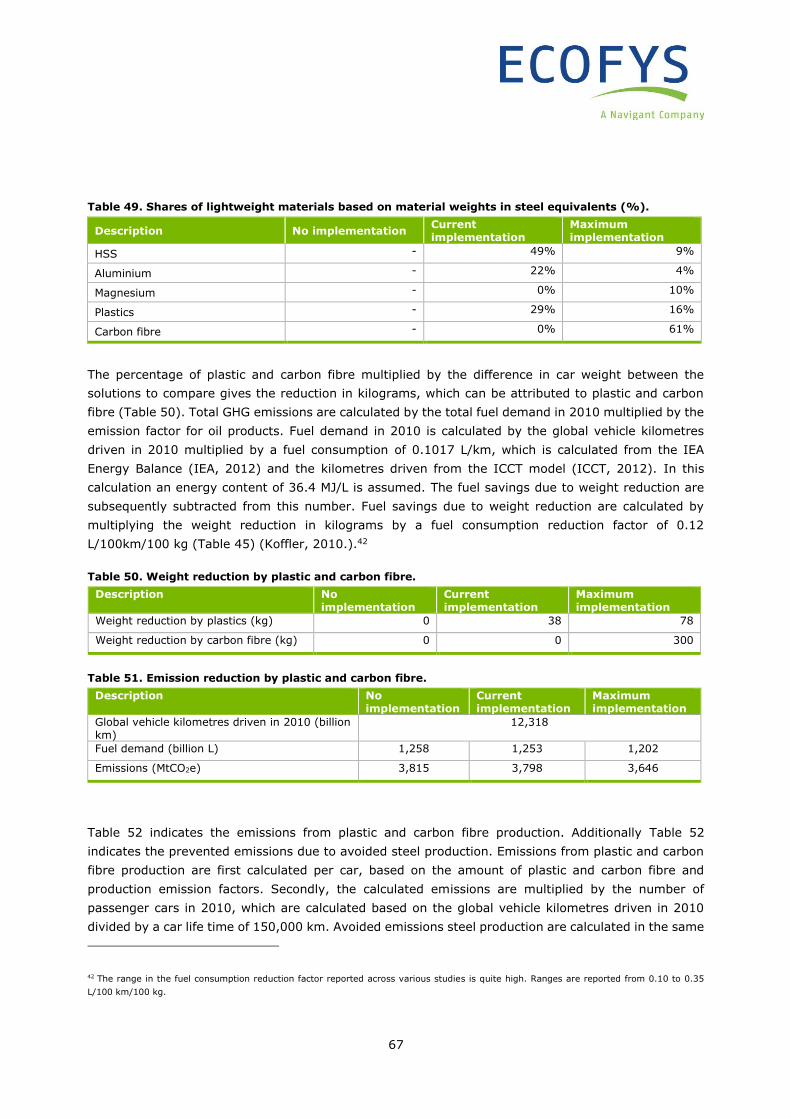
67
Table 49. Shares of lightweight materials based on material weights in steel equivalents (%).
Description No implementation Current implementation
Maximum implementation
HSS - 49% 9%
Aluminium - 22% 4%
Magnesium - 0% 10%
Plastics - 29% 16%
Carbon fibre - 0% 61%
The percentage of plastic and carbon fibre multiplied by the difference in car weight between the
solutions to compare gives the reduction in kilograms, which can be attributed to plastic and carbon
fibre (Table 50). Total GHG emissions are calculated by the total fuel demand in 2010 multiplied by the
emission factor for oil products. Fuel demand in 2010 is calculated by the global vehicle kilometres
driven in 2010 multiplied by a fuel consumption of 0.1017 L/km, which is calculated from the IEA
Energy Balance (IEA, 2012) and the kilometres driven from the ICCT model (ICCT, 2012). In this
calculation an energy content of 36.4 MJ/L is assumed. The fuel savings due to weight reduction are
subsequently subtracted from this number. Fuel savings due to weight reduction are calculated by
multiplying the weight reduction in kilograms by a fuel consumption reduction factor of 0.12
L/100km/100 kg (Table 45) (Koffler, 2010.).42
Table 50. Weight reduction by plastic and carbon fibre.
Description No implementation
Current implementation
Maximum implementation
Weight reduction by plastics (kg) 0 38 78
Weight reduction by carbon fibre (kg) 0 0 300
Table 51. Emission reduction by plastic and carbon fibre.
Description No implementation
Current implementation
Maximum implementation
Global vehicle kilometres driven in 2010 (billion km)
12,318
Fuel demand (billion L) 1,258 1,253 1,202
Emissions (MtCO2e) 3,815 3,798 3,646
Table 52 indicates the emissions from plastic and carbon fibre production. Additionally Table 52
indicates the prevented emissions due to avoided steel production. Emissions from plastic and carbon
fibre production are first calculated per car, based on the amount of plastic and carbon fibre and
production emission factors. Secondly, the calculated emissions are multiplied by the number of
passenger cars in 2010, which are calculated based on the global vehicle kilometres driven in 2010
divided by a car life time of 150,000 km. Avoided emissions steel production are calculated in the same
42 The range in the fuel consumption reduction factor reported across various studies is quite high. Ranges are reported from 0.10 to 0.35
L/100 km/100 kg.
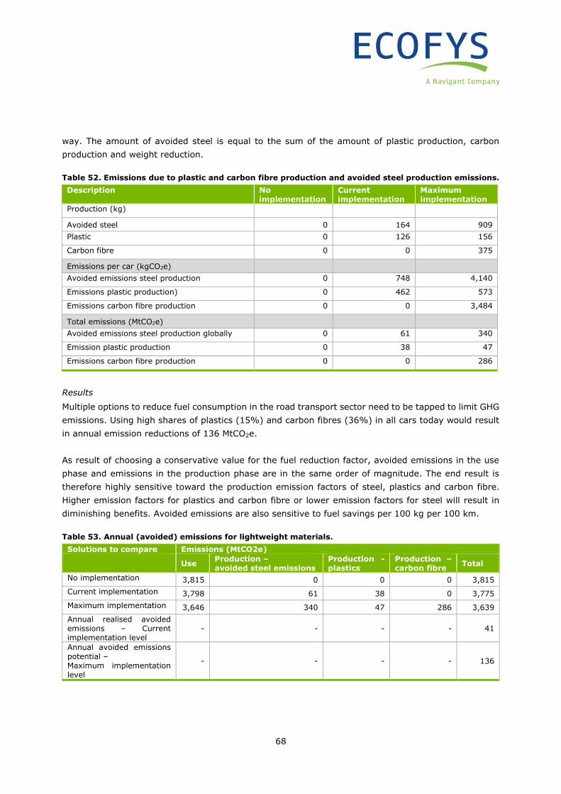
68
way. The amount of avoided steel is equal to the sum of the amount of plastic production, carbon
production and weight reduction.
Table 52. Emissions due to plastic and carbon fibre production and avoided steel production emissions.
Description No implementation
Current implementation
Maximum implementation
Production (kg)
Avoided steel 0 164 909
Plastic 0 126 156
Carbon fibre 0 0 375
Emissions per car (kgCO2e)
Avoided emissions steel production 0 748 4,140
Emissions plastic production) 0 462 573
Emissions carbon fibre production 0 0 3,484
Total emissions (MtCO2e)
Avoided emissions steel production globally 0 61 340
Emission plastic production 0 38 47
Emissions carbon fibre production 0 0 286
Results
Multiple options to reduce fuel consumption in the road transport sector need to be tapped to limit GHG
emissions. Using high shares of plastics (15%) and carbon fibres (36%) in all cars today would result
in annual emission reductions of 136 MtCO2e.
As result of choosing a conservative value for the fuel reduction factor, avoided emissions in the use
phase and emissions in the production phase are in the same order of magnitude. The end result is
therefore highly sensitive toward the production emission factors of steel, plastics and carbon fibre.
Higher emission factors for plastics and carbon fibre or lower emission factors for steel will result in
diminishing benefits. Avoided emissions are also sensitive to fuel savings per 100 kg per 100 km.
Table 53. Annual (avoided) emissions for lightweight materials.
Solutions to compare Emissions (MtCO2e)
Use
Production – avoided steel emissions
Production - plastics
Production – carbon fibre
Total
No implementation 3,815 0 0 0 3,815
Current implementation 3,798 61 38 0 3,775
Maximum implementation 3,646 340 47 286 3,639
Annual realised avoided emissions – Current implementation level
- - - - 41
Annual avoided emissions potential – Maximum implementation level
- - - - 136
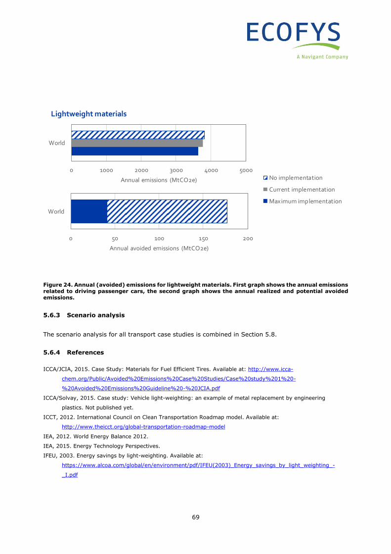
69
Figure 24. Annual (avoided) emissions for lightweight materials. First graph shows the annual emissions related to driving passenger cars, the second graph shows the annual realized and potential avoided emissions.
5.6.3 Scenario analysis
The scenario analysis for all transport case studies is combined in Section 5.8.
5.6.4 References
ICCA/JCIA, 2015. Case Study: Materials for Fuel Efficient Tires. Available at: http://www.icca-
chem.org/Public/Avoided%20Emissions%20Case%20Studies/Case%20study%201%20-
%20Avoided%20Emissions%20Guideline%20-%20JCIA.pdf
ICCA/Solvay, 2015. Case study: Vehicle light-weighting: an example of metal replacement by engineering
plastics. Not published yet.
ICCT, 2012. International Council on Clean Transportation Roadmap model. Available at:
http://www.theicct.org/global-transportation-roadmap-model
IEA, 2012. World Energy Balance 2012.
IEA, 2015. Energy Technology Perspectives.
IFEU, 2003. Energy savings by light-weighting. Available at:
https://www.alcoa.com/global/en/environment/pdf/IFEU(2003)_Energy_savings_by_light_weighting_-
_I.pdf
0 1000 2000 3000 4000 5000
World
Annual emissions (MtCO2e)
Lightweight materials
No implementation
Current implementation
Maximum implementation
0 50 100 150 200
World
Annual avoided emissions (MtCO2e)
70
Koffler, C., Rohde-Brandenburger, K., 2010. On the calculation of fuel savings through lightweight design in
automotive life cycle assessment. In: Environmental science & technology, 47, p12632-12647.
McKinsey, 2012. Lightweight, heavy impact: How carbon fibre and other lightweight materials will develop across
industries and specifically in automotive.
Zhang, X., M. Yamauchi, and J. Takahashi, 2011. "Life Cycle Assessment of CFRP in Application of Automobile."
18th International Conference on Composite Material. Available at: http://www.iccm-
central.org/Proceedings/ICCM18proceedings/data/2.%20Oral%20Presentation/Aug25(Thursday)/Th44%20
High%20Performance%20and%20Sustainable%20Composite%20Materials/Th44-3-AF1668.pdf
5.7 Transport: Electric cars
5.7.1 Contribution of chemical industry
Multiple options to reduce fuel consumption in the road transport sector need to be tapped to limit
global warming. Emission reductions can be enabled by transport demand reductions, but also by
efficient technologies, such as fuel efficient tires, lightweight materials and electric cars. Electrification
of road transport enables deep decarbonisation of the energy demand, because renewable electricity
can be supplied on a large scale. Furthermore, electric cars have a higher energy efficiency compared
to cars with conventional combustion engines. Chemical products play a key role in the production of
batteries required for electric cars. These include anode materials , cathode materials, electrolyte and
separators.
5.7.2 Avoided emissions potential calculation
Functional unit
The selected functional unit is driving passenger cars in the world in 2010, which is equal to
12,318 billion kilometres by light duty vehicles for passenger transport (ICCT, 2012). The potential
avoided emissions are calculated by the difference in life cycle GHG emissions for full electric vehicles
and the baseline (the current mix of electric and non-electric vehicles).
Solutions to compare
Three solutions to compare are identified, including no implementation, current implementation and
maximum implementation of electric vehicles (Table 54). The study calculates the already realized
avoided emissions by comparing the current mix of electric and non-electric vehicles (i.e. current
implementation) with the reference situation of no electric vehicles (i.e. no implementation). The
maximum potential for avoided emissions is calculated by comparing a hypothetical situation with a
maximum share of electric vehicles (i.e. maximum implementation) with the current implementation
of electric vehicles in the market. In reality the maximum share of electric vehicles will depend on a
range of factors of which amongst others the availability of rare earth metals.
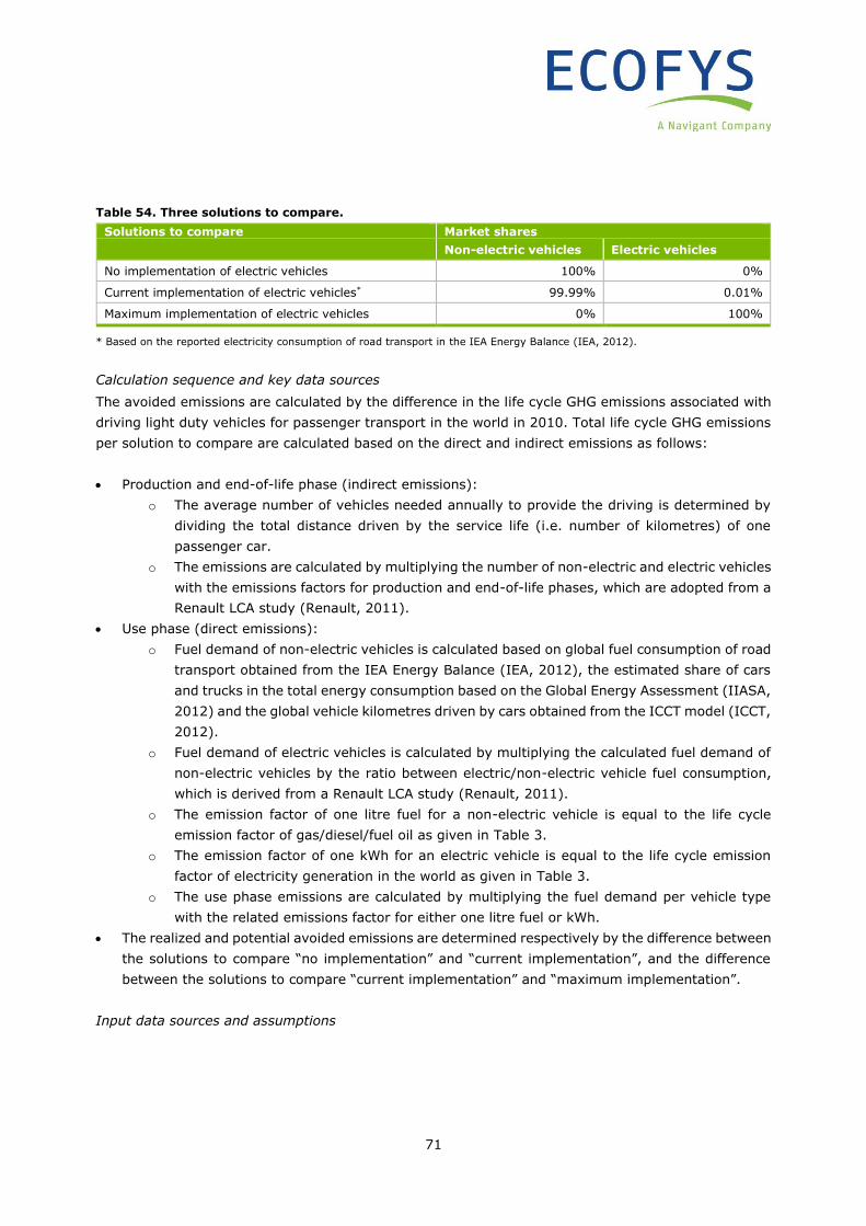
71
Table 54. Three solutions to compare.
Solutions to compare Market shares
Non-electric vehicles Electric vehicles
No implementation of electric vehicles 100% 0%
Current implementation of electric vehicles* 99.99% 0.01%
Maximum implementation of electric vehicles 0% 100%
* Based on the reported electricity consumption of road transport in the IEA Energy Balance (IEA, 2012).
Calculation sequence and key data sources
The avoided emissions are calculated by the difference in the life cycle GHG emissions associated with
driving light duty vehicles for passenger transport in the world in 2010. Total life cycle GHG emissions
per solution to compare are calculated based on the direct and indirect emissions as follows:
• Production and end-of-life phase (indirect emissions):
o The average number of vehicles needed annually to provide the driving is determined by
dividing the total distance driven by the service life (i.e. number of kilometres) of one
passenger car.
o The emissions are calculated by multiplying the number of non-electric and electric vehicles
with the emissions factors for production and end-of-life phases, which are adopted from a
Renault LCA study (Renault, 2011).
• Use phase (direct emissions):
o Fuel demand of non-electric vehicles is calculated based on global fuel consumption of road
transport obtained from the IEA Energy Balance (IEA, 2012), the estimated share of cars
and trucks in the total energy consumption based on the Global Energy Assessment (IIASA,
2012) and the global vehicle kilometres driven by cars obtained from the ICCT model (ICCT,
2012).
o Fuel demand of electric vehicles is calculated by multiplying the calculated fuel demand of
non-electric vehicles by the ratio between electric/non-electric vehicle fuel consumption,
which is derived from a Renault LCA study (Renault, 2011).
o The emission factor of one litre fuel for a non-electric vehicle is equal to the life cycle
emission factor of gas/diesel/fuel oil as given in Table 3.
o The emission factor of one kWh for an electric vehicle is equal to the life cycle emission
factor of electricity generation in the world as given in Table 3.
o The use phase emissions are calculated by multiplying the fuel demand per vehicle type
with the related emissions factor for either one litre fuel or kWh.
• The realized and potential avoided emissions are determined respectively by the difference between
the solutions to compare “no implementation” and “current implementation”, and the difference
between the solutions to compare “current implementation” and “maximum implementation”.
Input data sources and assumptions
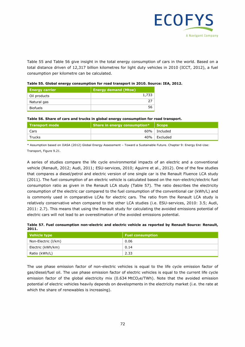
72
Table 55 and Table 56 give insight in the total energy consumption of cars in the world. Based on a
total distance driven of 12,317 billion kilometres for light duty vehicles in 2010 (ICCT, 2012), a fuel
consumption per kilometre can be calculated.
Table 55. Global energy consumption for road transport in 2010. Source: IEA, 2012.
Energy carrier Energy demand (Mtoe)
Oil products 1,733
Natural gas 27
Biofuels 56
Table 56. Share of cars and trucks in global energy consumption for road transport.
Transport mode Share in energy consumption* Scope
Cars 60% Included
Trucks 40% Excluded
* Assumption based on IIASA (2012) Global Energy Assessment – Toward a Sustainable Future. Chapter 9: Energy End-Use:
Transport, Figure 9.21.
A series of studies compare the life cycle environmental impacts of an electric and a conventional
vehicle (Renault, 2012; Audi, 2011; ESU-services, 2010; Aguirre et al., 2012). One of the few studies
that compares a diesel/petrol and electric version of one single car is the Renault Fluence LCA study
(2011). The fuel consumption of an electric vehicle is calculated based on the non-electric/electric fuel
consumption ratio as given in the Renault LCA study (Table 57). The ratio describes the electricity
consumption of the electric car compared to the fuel consumption of the conventional car (kWh/L) and
is commonly used in comparative LCAs for electric cars. The ratio from the Renault LCA study is
relatively conservative when compared to the other LCA studies (i.e. ESU-services, 2010: 3.5; Audi,
2011: 2.7). This means that using the Renault study for calculating the avoided emissions potential of
electric cars will not lead to an overestimation of the avoided emissions potential.
Table 57. Fuel consumption non-electric and electric vehicle as reported by Renault Source: Renault, 2011.
Vehicle type Fuel consumption
Non-Electric (l/km) 0.06
Electric (kWh/km) 0.14
Ratio (kWh/L) 2.33
The use phase emission factor of non-electric vehicles is equal to the life cycle emission factor of
gas/diesel/fuel oil. The use phase emission factor of electric vehicles is equal to the current life cycle
emission factor of the global electricity mix (0.634 MtCO2e/TWh). Note that the avoided emission
potential of electric vehicles heavily depends on developments in the electricity market (i.e. the rate at
which the share of renewables is increasing).
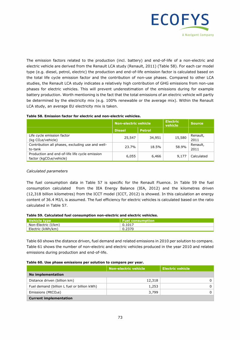
73
The emission factors related to the production (incl. battery) and end-of-life of a non-electric and
electric vehicle are derived from the Renault LCA study (Renault, 2011) (Table 58). For each car model
type (e.g. diesel, petrol, electric) the production and end-of-life emission factor is calculated based on
the total life cycle emission factor and the contribution of non-use phases. Compared to other LCA
studies, the Renault LCA study indicates a relatively high contribution of GHG emissions from non-use
phases for electric vehicles. This will prevent underestimation of the emissions during for example
battery production. Worth mentioning is the fact that the total emissions of an electric vehicle will partly
be determined by the electricity mix (e.g. 100% renewable or the average mix). Within the Renault
LCA study, an average EU electricity mix is taken.
Table 58. Emission factor for electric and non-electric vehicles.
Non-electric vehicle Electric vehicle
Source
Diesel Petrol
Life cycle emission factor
(kg CO2e/vehicle) 25,547 34,951 15,580
Renault,
2011
Contribution all phases, excluding use and well-
to-tank 23.7% 18.5% 58.9%
Renault,
2011
Production and end-of-life life cycle emission
factor (kgCO2e/vehicle) 6,055 6,466 9,177 Calculated
Calculated parameters
The fuel consumption data in Table 57 is specific for the Renault Fluence. In Table 59 the fuel
consumption calculated from the IEA Energy Balance (IEA, 2012) and the kilometres driven
(12,318 billion kilometres) from the ICCT model (ICCT, 2012) is showed. In this calculation an energy
content of 36.4 MJ/L is assumed. The fuel efficiency for electric vehicles is calculated based on the ratio
calculated in Table 57.
Table 59. Calculated fuel consumption non-electric and electric vehicles.
Vehicle type Fuel consumption
Non-Electric (l/km) 0.1017
Electric (kWh/km) 0.2370
Table 60 shows the distance driven, fuel demand and related emissions in 2010 per solution to compare.
Table 61 shows the number of non-electric and electric vehicles produced in the year 2010 and related
emissions during production and end-of-life.
Table 60. Use phase emissions per solution to compare per year.
Non-electric vehicle Electric vehicle
No implementation
Distance driven (billion km) 12,318 0
Fuel demand (billion L fuel or billion kWh) 1,253 0
Emissions (MtCO2e) 3,799 0
Current implementation
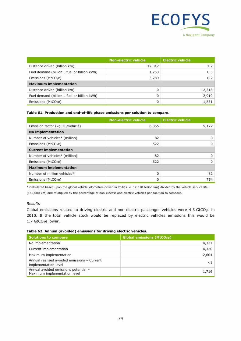
74
Non-electric vehicle Electric vehicle
Distance driven (billion km) 12,317 1.2
Fuel demand (billion L fuel or billion kWh) 1,253 0.3
Emissions (MtCO2e) 3,789 0.2
Maximum implementation
Distance driven (billion km) 0 12,318
Fuel demand (billion L fuel or billion kWh) 0 2,919
Emissions (MtCO2e) 0 1,851
Table 61. Production and end-of-life phase emissions per solution to compare.
Non-electric vehicle Electric vehicle
Emission factor (kgCO2/vehicle) 6,355 9,177
No implementation
Number of vehicles* (million) 82 0
Emissions (MtCO2e) 522 0
Current implementation
Number of vehicles* (million) 82 0
Emissions (MtCO2e) 522 0
Maximum implementation
Number of million vehicles* 0 82
Emissions (MtCO2e) 0 754
* Calculated based upon the global vehicle kilometres driven in 2010 (i.e. 12,318 billion km) divided by the vehicle service life
(150,000 km) and multiplied by the percentage of non-electric and electric vehicles per solution to compare.
Results
Global emissions related to driving electric and non-electric passenger vehicles were 4.3 GtCO2e in
2010. If the total vehicle stock would be replaced by electric vehicles emissions this would be
1.7 GtCO2e lower.
Table 62. Annual (avoided) emissions for driving electric vehicles.
Solutions to compare Global emissions (MtCO2e)
No implementation 4,321
Current implementation 4,320
Maximum implementation 2,604
Annual realised avoided emissions – Current
implementation level <1
Annual avoided emissions potential – Maximum implementation level
1,716
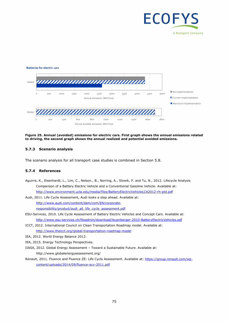
75
Figure 25. Annual (avoided) emissions for electric cars. First graph shows the annual emissions related to driving, the second graph shows the annual realized and potential avoided emissions.
5.7.3 Scenario analysis
The scenario analysis for all transport case studies is combined in Section 5.8.
5.7.4 References
Aguirre, K., Eisenhardt, L., Lim, C., Nelson., B., Norring, A., Slowik, P. and Tu, N., 2012. Lifecycle Analysis
Comparison of a Battery Electric Vehicle and a Conventional Gasoline Vehicle. Available at:
http://www.environment.ucla.edu/media/files/BatteryElectricVehicleLCA2012-rh-ptd.pdf
Audi, 2011. Life Cycle Assessment, Audi looks a step ahead. Available at:
http://www.audi.com/content/dam/com/EN/corporate-
responsibility/product/audi_a6_life_cycle_assessment.pdf
ESU-Services, 2010. Life Cycle Assessment of Battery Electric Vehicles and Concept Cars. Available at:
http://www.esu-services.ch/fileadmin/download/leuenberger-2010-BatteryElectricVehicles.pdf
ICCT, 2012. International Council on Clean Transportation Roadmap model. Available at:
http://www.theicct.org/global-transportation-roadmap-model
IEA, 2012. World Energy Balance 2012.
IEA, 2015. Energy Technology Perspectives.
IIASA, 2012. Global Energy Assessment – Toward a Sustainable Future. Available at:
http://www.globalenergyassessment.org/
Renault, 2011. Fluence and Fluence ZE: Life Cycle Assessment. Available at: https://group.renault.com/wp-
content/uploads/2014/09/fluence-acv-2011.pdf
0 500 1000 1500 2000 2500 3000 3500 4000 4500 5000
Global
Annual emissions (MtCO2e)
Batteries for electric cars
No implementation
Current implementation
Maximum implementation
0 200 400 600 800 1000 1200 1400 1600 1800
Global
Annual avoided emissions (MtCO2e)
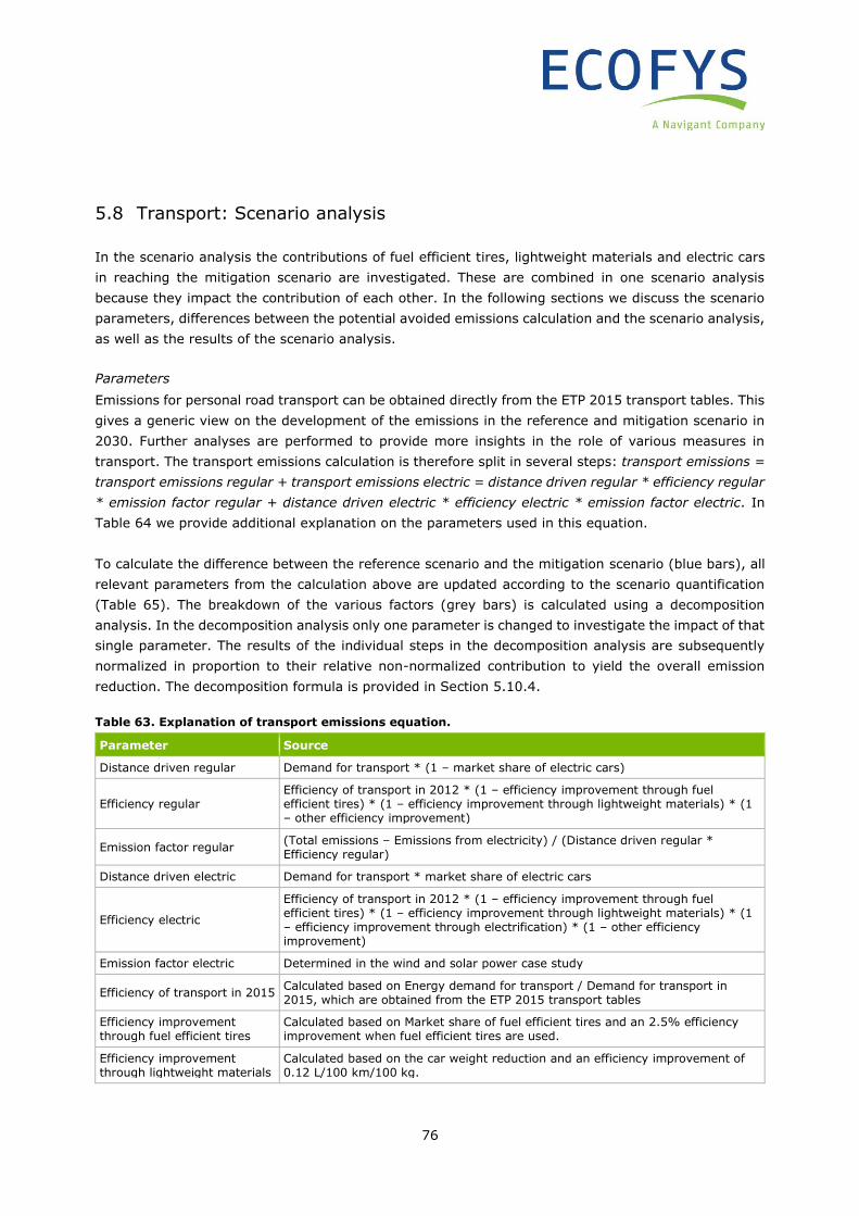
76
5.8 Transport: Scenario analysis
In the scenario analysis the contributions of fuel efficient tires, lightweight materials and electric cars
in reaching the mitigation scenario are investigated. These are combined in one scenario analysis
because they impact the contribution of each other. In the following sections we discuss the scenario
parameters, differences between the potential avoided emissions calculation and the scenario analysis,
as well as the results of the scenario analysis.
Parameters
Emissions for personal road transport can be obtained directly from the ETP 2015 transport tables. This
gives a generic view on the development of the emissions in the reference and mitigation scenario in
2030. Further analyses are performed to provide more insights in the role of various measures in
transport. The transport emissions calculation is therefore split in several steps: transport emissions =
transport emissions regular + transport emissions electric = distance driven regular * efficiency regular
* emission factor regular + distance driven electric * efficiency electric * emission factor electric. In
Table 64 we provide additional explanation on the parameters used in this equation.
To calculate the difference between the reference scenario and the mitigation scenario (blue bars), all
relevant parameters from the calculation above are updated according to the scenario quantification
(Table 65). The breakdown of the various factors (grey bars) is calculated using a decomposition
analysis. In the decomposition analysis only one parameter is changed to investigate the impact of that
single parameter. The results of the individual steps in the decomposition analysis are subsequently
normalized in proportion to their relative non-normalized contribution to yield the overall emission
reduction. The decomposition formula is provided in Section 5.10.4.
Table 63. Explanation of transport emissions equation.
Parameter Source
Distance driven regular Demand for transport * (1 – market share of electric cars)
Efficiency regular Efficiency of transport in 2012 * (1 – efficiency improvement through fuel efficient tires) * (1 – efficiency improvement through lightweight materials) * (1 – other efficiency improvement)
Emission factor regular (Total emissions – Emissions from electricity) / (Distance driven regular * Efficiency regular)
Distance driven electric Demand for transport * market share of electric cars
Efficiency electric
Efficiency of transport in 2012 * (1 – efficiency improvement through fuel efficient tires) * (1 – efficiency improvement through lightweight materials) * (1 – efficiency improvement through electrification) * (1 – other efficiency improvement)
Emission factor electric Determined in the wind and solar power case study
Efficiency of transport in 2015 Calculated based on Energy demand for transport / Demand for transport in 2015, which are obtained from the ETP 2015 transport tables
Efficiency improvement through fuel efficient tires
Calculated based on Market share of fuel efficient tires and an 2.5% efficiency improvement when fuel efficient tires are used.
Efficiency improvement through lightweight materials
Calculated based on the car weight reduction and an efficiency improvement of 0.12 L/100 km/100 kg.
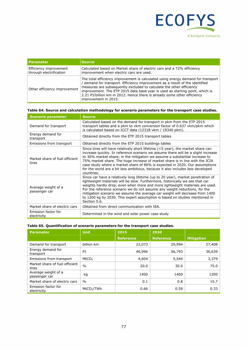
77
Parameter Source
Efficiency improvement through electrification
Calculated based on Market share of electric cars and a 72% efficiency improvement when electric cars are used.
Other efficiency improvement
The total efficiency improvement is calculated using energy demand for transport / demand for transport. Efficiency improvement as a result of the identified measures are subsequently excluded to calculate the other efficiency improvement. The ETP 2015 data base year is used as starting point, which is 2.21 PJ/billion km in 2012. Hence there is already some other efficiency improvement in 2015.
Table 64. Source and calculation methodology for scenario parameters for the transport case studies.
Scenario parameter Source
Demand for transport Calculated based on the demand for transport in pkm from the ETP 2015 transport tables and a pkm to vkm conversion factor of 0.637 vkm/pkm which is calculated based on ICCT data (12318 vkm / 19340 pkm).
Energy demand for transport
Obtained directly from the ETP 2015 transport tables
Emissions from transport Obtained directly from the ETP 2015 buildings tables
Market share of fuel efficient tires
Since tires will have relatively short lifetime (<5 year), the market share can increase quickly. In reference scenario we assume there will be a slight increase to 30% market share; in the mitigation we assume a substantial increase to 75% market share. The huge increase of market share is in line with the JCIA case study where a market share of 86% is expected in 2020. Our assumptions for the world are a bit less ambitious, because it also includes less developed countries.
Average weight of a passenger car
Since car have a relatively long lifetime (up to 20 year), market penetration of lightweight materials will be slow. Furthermore, historically we see that car weights hardly drop, even when more and more lightweight materials are used. For the reference scenario we do not assume any weight reductions, for the mitigation scenario we assume the average car weight will decrease from 1400 to 1200 kg by 2030. This expert assumption is based on studies mentioned in Section 5.6.
Market share of electric cars Obtained from direct communication with IEA.
Emission factor for electricity
Determined in the wind and solar power case study
Table 65. Quantification of scenario parameters for the transport case studies.
Parameter Unit 2015 2030
Reference Reference Mitigation
Demand for transport billion km 22,073 29,994 27,408
Energy demand for transport
PJ 46,996 56,793 36,639
Emissions from transport MtCO2 4,604 5,544 3,379
Market share of fuel efficient tires
% 20.0 30.0 75.0
Average weight of a passenger car
kg 1400 1400 1200
Market share of electric cars % 0.1 0.8 15.7
Emission factor for electricity
MtCO2/TWh 0.66 0.59 0.33
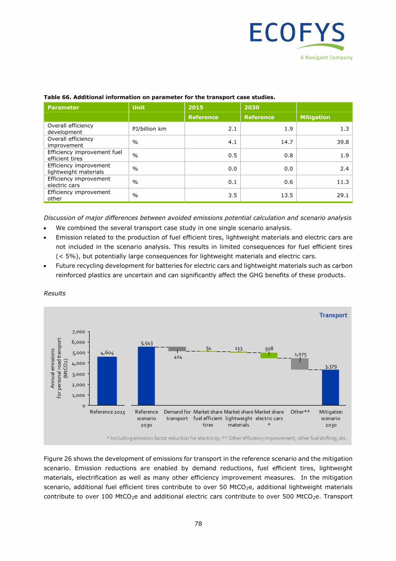
78
Table 66. Additional information on parameter for the transport case studies.
Parameter Unit 2015 2030
Reference Reference Mitigation
Overall efficiency development
PJ/billion km 2.1 1.9 1.3
Overall efficiency improvement
% 4.1 14.7 39.8
Efficiency improvement fuel efficient tires
% 0.5 0.8 1.9
Efficiency improvement lightweight materials
% 0.0 0.0 2.4
Efficiency improvement electric cars
% 0.1 0.6 11.3
Efficiency improvement other
% 3.5 13.5 29.1
Discussion of major differences between avoided emissions potential calculation and scenario analysis
• We combined the several transport case study in one single scenario analysis.
• Emission related to the production of fuel efficient tires, lightweight materials and electric cars are
not included in the scenario analysis. This results in limited consequences for fuel efficient tires
(< 5%), but potentially large consequences for lightweight materials and electric cars.
• Future recycling development for batteries for electric cars and lightweight materials such as carbon
reinforced plastics are uncertain and can significantly affect the GHG benefits of these products.
Results
Figure 26 shows the development of emissions for transport in the reference scenario and the mitigation
scenario. Emission reductions are enabled by demand reductions, fuel efficient tires, lightweight
materials, electrification as well as many other efficiency improvement measures. In the mitigation
scenario, additional fuel efficient tires contribute to over 50 MtCO2e, additional lightweight materials
contribute to over 100 MtCO2e and additional electric cars contribute to over 500 MtCO2e. Transport
Transport
3,379
1,07550811354
414
5,543
Mitigation scenario
2030
Market share electric cars
*
Other**Demand for transport
Reference scenario
2030
Market share fuel efficient
tires
Market share lightweight
materials
3,000
2,000
7,000
6,000
4,000
5,000
1,000
0Reference 2015
4,604
An
nu
al e
mis
sio
ns
for
per
son
al r
oad
tran
spor
t(M
tCO
2)
* Including emission factor reduction for electricity; ** Other efficiency improvement, other fuel shifting, etc.
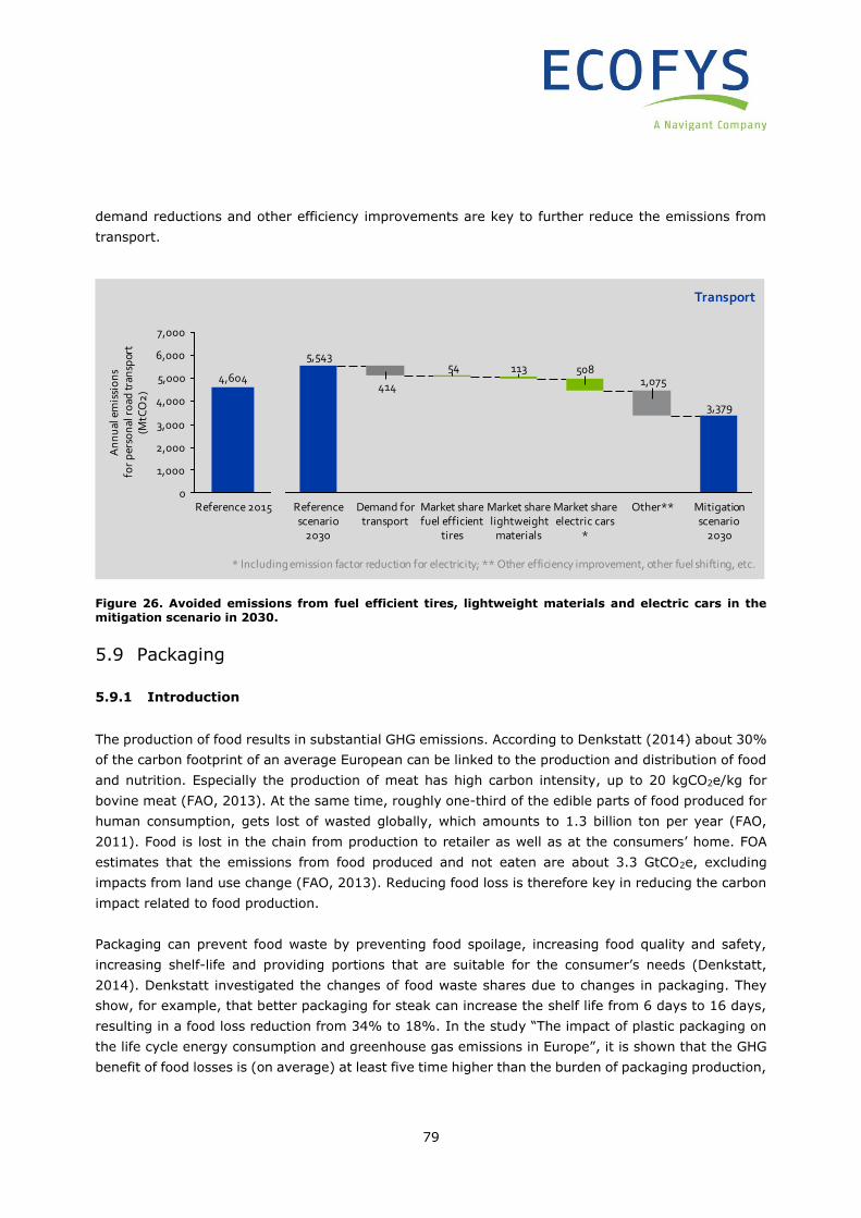
79
demand reductions and other efficiency improvements are key to further reduce the emissions from
transport.
Figure 26. Avoided emissions from fuel efficient tires, lightweight materials and electric cars in the mitigation scenario in 2030.
5.9 Packaging
5.9.1 Introduction
The production of food results in substantial GHG emissions. According to Denkstatt (2014) about 30%
of the carbon footprint of an average European can be linked to the production and distribution of food
and nutrition. Especially the production of meat has high carbon intensity, up to 20 kgCO2e/kg for
bovine meat (FAO, 2013). At the same time, roughly one-third of the edible parts of food produced for
human consumption, gets lost of wasted globally, which amounts to 1.3 billion ton per year (FAO,
2011). Food is lost in the chain from production to retailer as well as at the consumers’ home. FOA
estimates that the emissions from food produced and not eaten are about 3.3 GtCO2e, excluding
impacts from land use change (FAO, 2013). Reducing food loss is therefore key in reducing the carbon
impact related to food production.
Packaging can prevent food waste by preventing food spoilage, increasing food quality and safety,
increasing shelf-life and providing portions that are suitable for the consumer’s needs (Denkstatt,
2014). Denkstatt investigated the changes of food waste shares due to changes in packaging. They
show, for example, that better packaging for steak can increase the shelf life from 6 days to 16 days,
resulting in a food loss reduction from 34% to 18%. In the study “The impact of plastic packaging on
the life cycle energy consumption and greenhouse gas emissions in Europe”, it is shown that the GHG
benefit of food losses is (on average) at least five time higher than the burden of packaging production,
Transport
3,379
1,07550811354
414
5,543
Mitigation scenario
2030
Market share electric cars
*
Other**Demand for transport
Reference scenario
2030
Market share fuel efficient
tires
Market share lightweight
materials
3,000
2,000
7,000
6,000
4,000
5,000
1,000
0Reference 2015
4,604
An
nu
al e
mis
sio
ns
for
per
son
al r
oad
tran
spor
t(M
tCO
2)
* Including emission factor reduction for electricity; ** Other efficiency improvement, other fuel shifting, etc.
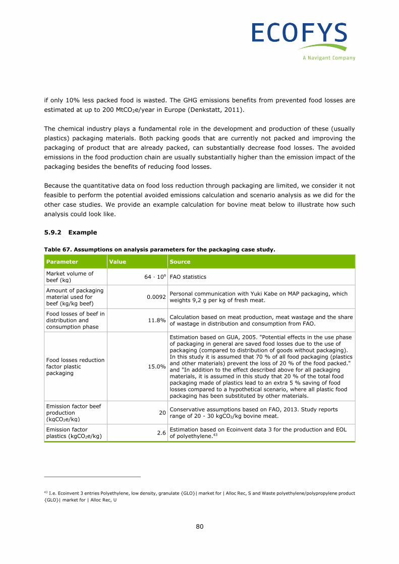
80
if only 10% less packed food is wasted. The GHG emissions benefits from prevented food losses are
estimated at up to 200 MtCO2e/year in Europe (Denkstatt, 2011).
The chemical industry plays a fundamental role in the development and production of these (usually
plastics) packaging materials. Both packing goods that are currently not packed and improving the
packaging of product that are already packed, can substantially decrease food losses. The avoided
emissions in the food production chain are usually substantially higher than the emission impact of the
packaging besides the benefits of reducing food losses.
Because the quantitative data on food loss reduction through packaging are limited, we consider it not
feasible to perform the potential avoided emissions calculation and scenario analysis as we did for the
other case studies. We provide an example calculation for bovine meat below to illustrate how such
analysis could look like.
5.9.2 Example
Table 67. Assumptions on analysis parameters for the packaging case study.
Parameter Value Source
Market volume of beef (kg)
64 ∙ 109 FAO statistics
Amount of packaging material used for beef (kg/kg beef)
0.0092 Personal communication with Yuki Kabe on MAP packaging, which weights 9,2 g per kg of fresh meat.
Food losses of beef in distribution and consumption phase
11.8% Calculation based on meat production, meat wastage and the share of wastage in distribution and consumption from FAO.
Food losses reduction factor plastic packaging
15.0%
Estimation based on GUA, 2005. "Potential effects in the use phase of packaging in general are saved food losses due to the use of packaging (compared to distribution of goods without packaging). In this study it is assumed that 70 % of all food packaging (plastics and other materials) prevent the loss of 20 % of the food packed." and "In addition to the effect described above for all packaging materials, it is assumed in this study that 20 % of the total food packaging made of plastics lead to an extra 5 % saving of food losses compared to a hypothetical scenario, where all plastic food packaging has been substituted by other materials.
Emission factor beef production (kgCO2e/kg)
20 Conservative assumptions based on FAO, 2013. Study reports range of 20 - 30 kgCO2/kg bovine meat.
Emission factor plastics (kgCO2e/kg)
2.6 Estimation based on Ecoinvent data 3 for the production and EOL of polyethylene.43
43 I.e. Ecoinvent 3 entries Polyethylene, low density, granulate {GLO}| market for | Alloc Rec, S and Waste polyethylene/polypropylene product
{GLO}| market for | Alloc Rec, U
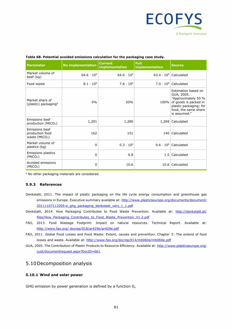
81
Table 68. Potential avoided emissions calculation for the packaging case study.
Parameter No implementation Current implementation
Full implementation
Source
Market volume of beef (kg)
64.6 ∙ 109 64.0 ∙ 109 63.4 ∙ 109 Calculated
Food waste 8.1 ∙ 109 7.6 ∙ 109 7.0 ∙ 109 Calculated
Market share of (plastic) packaginga
0% 50% 100%
Estimation based on GUA, 2005. "Approximately 50 % of goods is packed in plastic packaging; for food, the same share is assumed."
Emissions beef production (MtCO2)
1,291 1,280 1,269 Calculated
Emissions beef production food waste (MtCO2)
162 151 140 Calculated
Market volume of plastics (kg)
0 0.3 ∙ 109 0.6 ∙ 109 Calculated
Emissions plastics (MtCO2)
0 0.8 1.5 Calculated
Avoided emissions (MtCO2)
0 10.6 10.6 Calculated
a No other packaging materials are considered.
5.9.3 References
Denkstatt, 2011. The impact of plastic packaging on the life cycle energy consumption and greenhouse gas
emissions in Europe. Executive summary available at: http://www.plasticseurope.org/documents/document/
20111107113205-e_ghg_packaging_denkstatt_vers_1_1.pdf
Denkstatt, 2014. How Packaging Contributes to Food Waste Prevention. Available at: http://denkstatt.at/
files/How_Packaging_Contributes_to_Food_Waste_Prevention_V1.2.pdf
FAO, 2013. Food Wastage Footprint: Impact on natural resources. Technical Report. Available at:
http://www.fao.org/ docrep/018/ar429e/ar429e.pdf
FAO, 2011. Global Food Losses and Food Waste: Extent, causes and prevention. Chapter 3: The extend of food
losses and waste. Available at: http://www.fao.org/docrep/014/mb060e/mb060e.pdf
GUA, 2005. The Contribution of Plastic Products to Resource Efficiency. Available at: http://www.plasticseurope.org/
cust/documentrequest.aspx?DocID=661
5.10 Decomposition analysis
5.10.1 Wind and solar power
GHG emission by power generation is defined by a function G,
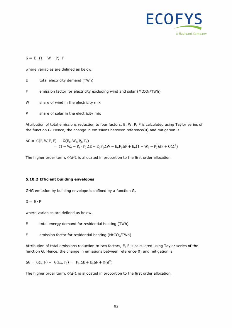
82
G = E ∙ (1 − W − P) ∙ F
where variables are defined as below.
E total electricity demand (TWh)
F emission factor for electricity excluding wind and solar (MtCO2/TWh)
W share of wind in the electricity mix
P share of solar in the electricity mix
Attribution of total emissions reduction to four factors, E, W, P, F is calculated using Taylor series of
the function G. Hence, the change in emissions between reference(0) and mitigation is
∆G = G(E, W, P, F) − G(E0, W0, P0, F0)
= (1 − W0 − P0) F0 ∆E − E0F0∆W − E0F0∆P + E0(1 − W0 − P0)∆F + O(∆2)
The higher order term, O(∆2), is allocated in proportion to the first order allocation.
5.10.2 Efficient building envelopes
GHG emission by building envelope is defined by a function G,
G = E ∙ F
where variables are defined as below.
E total energy demand for residential heating (TWh)
F emission factor for residential heating (MtCO2/TWh)
Attribution of total emissions reduction to two factors, E, F is calculated using Taylor series of the
function G. Hence, the change in emissions between reference(0) and mitigation is
∆G = G(E, F) − G(E0, F0) = F0 ∆E + E0∆F + O(∆2)
The higher order term, O(∆2), is allocated in proportion to the first order allocation.
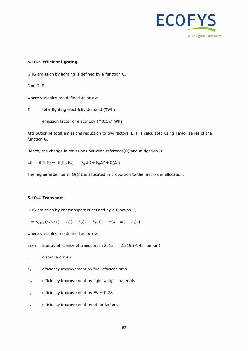
83
5.10.3 Efficient lighting
GHG emission by lighting is defined by a function G,
G = E ∙ F
where variables are defined as below.
E total lighting electricity demand (TWh)
F emission factor of electricity (MtCO2/TWh)
Attribution of total emissions reduction to two factors, E, F is calculated using Taylor series of the
function G.
Hence, the change in emissions between reference(0) and mitigation is
∆G = G(E, F) − G(E0, F0) = F0 ∆E + E0∆F + O(∆2)
The higher order term, O(∆2), is allocated in proportion to the first order allocation.
5.10.4 Transport
GHG emission by car transport is defined by a function G,
𝐺 = 𝐸2012 (𝐿 3.6⁄ )(1 − ℎ𝑡)(1 − ℎ𝑤)(1 − ℎ𝑥) {(1 − 𝑚)𝑘 + 𝑚(1 − ℎ𝑒)𝑧}
where variables are defined as below.
E2012 Energy efficiency of transport in 2012 = 2.219 (PJ/billion km)
L distance driven
ht efficiency improvement by fuel-efficient tires
hw efficiency improvement by light-weight materials
he efficiency improvement by EV = 0.78
hx efficiency improvement by other factors
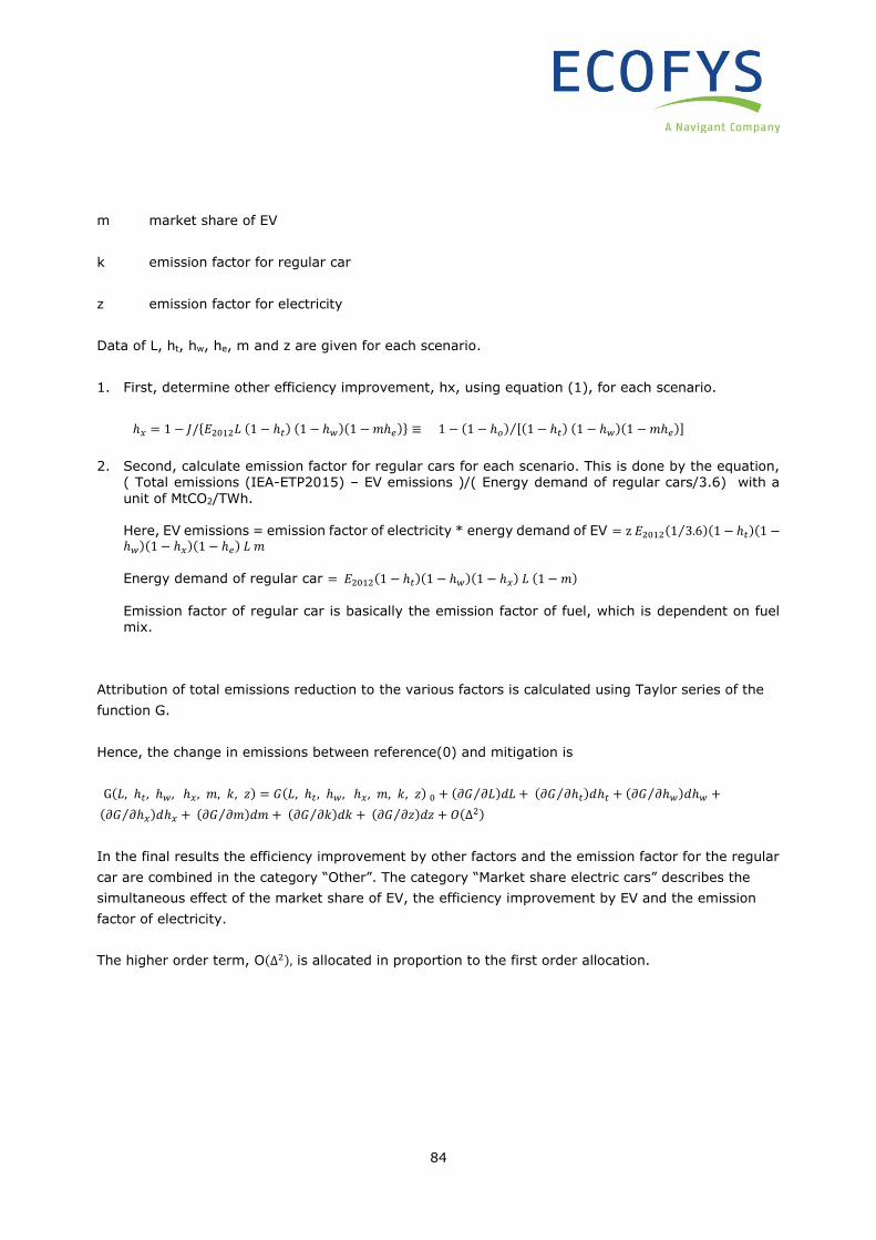
84
m market share of EV
k emission factor for regular car
z emission factor for electricity
Data of L, ht, hw, he, m and z are given for each scenario.
1. First, determine other efficiency improvement, hx, using equation (1), for each scenario.
ℎ𝑥 = 1 − 𝐽/{𝐸2012𝐿 (1 − ℎ𝑡) (1 − ℎ𝑤)(1 − 𝑚ℎ𝑒)} ≡ 1 − (1 − ℎ𝑜) [(1 − ℎ𝑡) (1 − ℎ𝑤)(1 − 𝑚ℎ𝑒)]⁄
2. Second, calculate emission factor for regular cars for each scenario. This is done by the equation, ( Total emissions (IEA-ETP2015) – EV emissions )/( Energy demand of regular cars/3.6) with a
unit of MtCO2/TWh. Here, EV emissions = emission factor of electricity * energy demand of EV = z 𝐸2012(1 3.6⁄ )(1 − ℎ𝑡)(1 −ℎ𝑤)(1 − ℎ𝑥)(1 − ℎ𝑒) 𝐿 𝑚
Energy demand of regular car = 𝐸2012(1 − ℎ𝑡)(1 − ℎ𝑤)(1 − ℎ𝑥) 𝐿 (1 − 𝑚) Emission factor of regular car is basically the emission factor of fuel, which is dependent on fuel mix.
Attribution of total emissions reduction to the various factors is calculated using Taylor series of the
function G.
Hence, the change in emissions between reference(0) and mitigation is
G(𝐿, ℎ𝑡, ℎ𝑤, ℎ𝑥, 𝑚, 𝑘, 𝑧) = 𝐺(𝐿, ℎ𝑡, ℎ𝑤, ℎ𝑥, 𝑚, 𝑘, 𝑧) 0 + (𝜕𝐺 𝜕𝐿⁄ )𝑑𝐿 + (𝜕𝐺 𝜕ℎ𝑡⁄ )𝑑ℎ𝑡 + (𝜕𝐺 𝜕ℎ𝑤⁄ )𝑑ℎ𝑤 +
(𝜕𝐺 𝜕ℎ𝑥⁄ )𝑑ℎ𝑥 + (𝜕𝐺 𝜕𝑚⁄ )𝑑𝑚 + (𝜕𝐺 𝜕𝑘⁄ )𝑑𝑘 + (𝜕𝐺 𝜕𝑧⁄ )𝑑𝑧 + 𝑂(∆2)
In the final results the efficiency improvement by other factors and the emission factor for the regular
car are combined in the category “Other”. The category “Market share electric cars” describes the
simultaneous effect of the market share of EV, the efficiency improvement by EV and the emission
factor of electricity.
The higher order term, O(∆2), is allocated in proportion to the first order allocation.


ECOFYS Netherlands B.V.
Kanaalweg 15G
3526 KL Utrecht
T: +31 (0) 30 662-3300
F: +31 (0) 30 662-3301
I: www.ecofys.com