Embed Size (px)
Citation preview

REDUCTION OF DISCRETE AND FINITE ELEMENT MODELS
USING BOUNDARY CHARACTERISTIC ORTHOGONAL VECTORS
Raghdan Joseph Al Khoury
A Thesis in
The Department of
Mechanical and Industrial Engineering
Presented in Partial Fulfillment of the Requirements for the
Degree of Master of Applied Science (mechanical engineering)
Concordia University
Montreal, Quebec
Canada
August 2008
© Raghdan Joseph Al Khoury, 2008

1*1 Library and Archives Canada
Published Heritage Branch
395 Wellington Street Ottawa ON K1A0N4 Canada
Bibliotheque et Archives Canada
Direction du Patrimoine de I'edition
395, rue Wellington Ottawa ON K1A0N4 Canada
Your file Votre reference ISBN: 978-0-494-45450-3 Our file Notre reference ISBN: 978-0-494-45450-3
NOTICE: The author has granted a nonexclusive license allowing Library and Archives Canada to reproduce, publish, archive, preserve, conserve, communicate to the public by telecommunication or on the Internet, loan, distribute and sell theses worldwide, for commercial or noncommercial purposes, in microform, paper, electronic and/or any other formats.
AVIS: L'auteur a accorde une licence non exclusive permettant a la Bibliotheque et Archives Canada de reproduire, publier, archiver, sauvegarder, conserver, transmettre au public par telecommunication ou par Plntemet, prefer, distribuer et vendre des theses partout dans le monde, a des fins commerciales ou autres, sur support microforme, papier, electronique et/ou autres formats.
The author retains copyright ownership and moral rights in this thesis. Neither the thesis nor substantial extracts from it may be printed or otherwise reproduced without the author's permission.
L'auteur conserve la propriete du droit d'auteur et des droits moraux qui protege cette these. Ni la these ni des extraits substantiels de celle-ci ne doivent etre imprimes ou autrement reproduits sans son autorisation.
In compliance with the Canadian Privacy Act some supporting forms may have been removed from this thesis.
Conformement a la loi canadienne sur la protection de la vie privee, quelques formulaires secondaires ont ete enleves de cette these.
While these forms may be included in the document page count, their removal does not represent any loss of content from the thesis.
Canada
Bien que ces formulaires aient inclus dans la pagination, il n'y aura aucun contenu manquant.

ABSTRACT
REDUCTION OF DISCRETE AND FINITE ELEMENT MODELS USING BOUNDARY
CHARACTERISTIC ORTHOGONAL VECTORS
Raghdan Joseph Al Khoury
Solution of large eigenvalue problems is time consuming. Large eigenvalue problems
of discrete models can occur in many cases, especially in Finite Element analysis of
structures with large number of degrees of freedom. Many studies have proposed
reduction of the size of eigenvalue problems which are quite well known today.
In the current study a survey of the existing model reduction methods is presented. A
new proposed method is formulated and compared with the earlier studies, namely, static
and dynamic condensation methods which are presented in detail. Many case studies are
presented.
The proposed model reduction method is based on the boundary characteristic
orthogonal polynomials in the Rayleigh-Ritz method. This method is extended to discrete
models and the admissible functions are replaced by vectors. Gram-Schmidt
orthogonalization was used in the first case study to generate the orthogonal vectors in
order to reduce a building model.
Further, a more general method is presented and it is mainly used to reduce FEM
models. Results have shown many advantages for the new method.
iii

A JINA, JOSEPH, ALAA ET SAMI
IV

Acknowledgments
I would like to express my gratitude towards my supervisor, Professor Rama B.
Bhat for his guidance and valuable advice. He was always a great help in the process of
developing my thesis.
1 would also like to acknowledge Dr. A. K. Waisuddin Ahmed for his guidance in
the beginning of my studies at Concordia University.
My gratitude must also go to Joe Hulet for always aiding me with my
technological problems. Finally, I would like to thank all my colleagues, especially my
lab mates for the beneficial discussions that we held and for the good times I experienced.
v

Table of Contents
List of Figures viii
List of Tables x
Nomenclature xi
Chapter 1 Introduction... 1
1.1. General information 1
1.2. The Rayleigh Ritz method 2
1.2. Boundary characteristic orthogonal polynomials 3
1.3. Model reduction 6
1.4. Objectives and scope of the research 10
1.6. Organization of the thesis 11
Chapter 2 Employing orthogonal vectors of model reduction for discrete systems. 13
2.1. Modeling 15
2.2. Characteristic orthogonal vector set 17
2.3. Results and discussion 20
2.4. Dynamic reduction 27
Chapter 3 Employing orthogonal vectors for model reduction of FEM models 31
3.1. Exact dynamic condensation 31
3.2. Static condensation 34
3.3. Boundary characteristic orthogonal vectors in the Rayleigh-Ritz analysis... 34
3.3.1. Modified Gram-Schmidt method 35
3.3.2. Boundary characteristic orthogonal vectors by static deflection ..37
3.4. Comparison of different model reduction techniques 40
3.5. Example structures 41
3.5.1. Cantilever beam 41
3.5.2. Simply supported beam 48
3.5.3. Clamped-clamped beam 49
vi

Chapter 4 Applications of the model reduction using orthogonal vectors set in the Rayleigh-Ritz method 53
4.1. Introduction 53
4.2. Harmonic analysis of vehicle reduced order model 54
4.3. Model reduction of a fluid filled pipe 60
4.3.1. Modeling using FEM .....61
4.3.2. Reduction of the model 64
Chapter 5 Using independent vectors for the reduction of generalized eigenvalue problem 70
5.1. The Rayleigh-Ritz method for plate vibrations 70
5.2. Assumed deflection shapes 73
5.3. Numerical result for elliptical plate ....78
Chapter 6 Conclusions and recommendations for future work 83
6.1. Thesis summary 83
6.2. Contributions , 85
6.3. Major conclusions 85
6.4. Future work 87
References 88
Appendix-A 94
vn

List of Figures
Fig. 1: Master DOF selection in a cantilever beam 8
Fig. 2. Multi-storey building model 15
Fig. 3. Vector # 1 vs. floors...... 21
Fig. 4. Vector # 2 vs. floors 22
Fig. 5. Vector # 3 vs. floors 22
Fig. 6. Vector # 4 vs. floors..... 23
Fig. 7. Vector # 5 vs. floors 23
Fig. 8. Vector # 6 vs. floors 24
Fig. 9.Transmissibility plots of the generalized coordinates 26
Fig. 10. Transmissibility plots of first and second generalized coordinates 28
Fig. 11. Transmissibility plots of the first, second and third generalized coordinates. 29
Fig.12: Algorithm for the generation of orthogonal vectors 38
Fig. 13: Computation scheme for the generation of orthogonal vectors 39
Fig. 14: Model of a cantilever beam 41
Fig. 15. Comparison of the first mode with assumed vectors 43
Fig. 16. Comparison of the second mode with assumed vectors 43
Fig. 17. Comparison of the third mode with assumed vectors 44
Fig. 18. Comparison of the fourth mode with assumed vectors 44
Fig. 19. Comparison of the fifth mode with assumed vectors 45
Fig. 20. Comparison of the first exact mode with assumed vectors 50
Fig. 21. Comparison of the third exact mode with assumed vectors 50
Fig. 22. Comparison of the fifth mode with assumed vectors 51
viii

Fig. 23. Vehicle body model with attached spring mass systems 54
Fig. 24. Node location of FEM model 55
Fig. 25. Transmissibility plots of the exact and reduced models 57
Fig. 26. Phase plots of the exact and reduced models 58
Fig. 27. Transmissibility plots of exact and reduced models 59
Fig. 28. Transmissibility plots of exact and reduced models 59
Fig. 29. Sketch of one bank of the coiled heat exchanger 60
Fig. 30. The simulation of the coil bank by a 3D curve 63
Fig. 31. Exact vs. meshed models 64
Fig. 32. Support locations 65
Fig. 33. Convergence history of 10th, 11th, 12th, and 13th modes 67
Fig. 34. Convergence history of 1st, 2nd, 3rd and 4th modes 68
Fig. 35. General plot of a rectangular plate with line supports 73
Fig. 36. Scheme of generating the linear independent basis 75
Fig. 37. Assumed mode shapes for elliptical and circular plates 79
Fig. 38. Mode shapes of circular platesa = 1 80
Fig. 39. Mode shape of elliptical platea = 2 80
IX

List of Tables
Table 1. Natural frequencies of the structure 24
Table 2. Reduced model natural frequencies 27
Table 3. Reduced model natural frequencies 27
Table 4: Transformation formulae for different methods 40
Table 5: Comparison between exact and reduced eigenvalues of both Modified Gram-Schmidt and Static load in the Rayleigh-Ritz method 42
Table 6: Comparison between the reduced eigenvalues of different reduction methods 47
Table 7: Comparison between the reduced eigenvalues of different reduction methods 48
Table 8: Comparison of natural frequencies of SS beam 49
Table 9: Comparison between the reduced natural frequencies of different methods for CC beam 51
Table 10: Numerical parameters 56
Table 11: Comparison of exact and reduced natural frequencies 57
Table 12: Parametric equations of the coil 62
Table 13: Geometry and parameters of the coil 64
Table 14: Eigenvalue of reduced (10 natural frequencies) and complete model 65
Table 15: Eigenvalue of reduced (20 natural frequencies) and complete model 66
Table 16: Comparison of the eigenvlaues of reduced and full models of circular platesa = l 81
Table 17: Comparison of the eigenvalues of reduced and full models of elliptical platesa = 2 81
x

Nomenclature
w w [M]
w [c] x b
14 M;
k/
c i
w" w IF) fD 1 L mm J
fD 1 L ms J
[DJ [Dj K] W [Kmm]
KJ PU K] Ka] K] [MJ K]
Normalized assumed deflection vector
Non normalized assumed deflection vector
Mass Matrix
Stiffness Matrix
Damping Matrix
Base excitation
Uniform load vector
Massofi thDOF
Stiffness coefficient of ith spring
Damping coefficient of il spring
Deflection vector
Dynamic matrix
Force vector
Master-master dynamic matrix
Master-slave dynamic matrix
Slave-master dynamic matrix
Slave-slave dynamic matrix
Master deflection
Slave deflection
Master-master Stiffness matrix
Master-slave stiffness matrix
Slave-master stiffness matrix
Slave-slave stiffness matrix
Deflection-deflection Mass matrix
Deflection-slope mass matrix
Slope-deflection mass matrix
Slope-slope mass matrix
XI

Deflection-deflection Stiffness matrix
Deflection-slope stiffness matrix
Slope-deflection stiffness matrix
Slope-slope stiffness matrix
ith deflection vector
ith slope vector
Generalized coordinate vector
Transformation matrix
Deflection function in term of JC and y
Young modulus Thickness of the plate Poisson's ratio Density
Maximum kinetic energy
Maximum potential energy
m* generalized coordinate
Non-dimensional eigenvalue
Non-dimensional abscissa
Non-dimensional ordinate
xn

Chapter 1
Introduction
1.1. General information
Real structures and systems can be modeled as either continuous or discrete or a
combination of both. The vibration behavior of such structures is studied by expressing
the vibratory motion in the form of differential equations that may be solved analytically
in some cases or using approximate methods in other. In general, discretization of a
continuous structure is a powerful method to solve the differential equations with
acceptable accuracy. Two of the well known methods are the Rayleigh-Ritz and the
Finite Element Method (FEM).
Briefly, FEM or FEA (finite element analysis) is a numerical method to solve partial
differential equations by transforming the problem into a set of ordinary differential
equations that can be solved using different numerical methods. FEM was first proposed
in 1941 and 1942, in order to solve structural problems. This method has evolved over
the years with many improvements and it forms now one of the most used methods to
simulate physical systems. This method can be used for the static and dynamic analysis,
where a continuous structure is discretized into a finite number of DOFs. Currently, a
variety of elements are used for the structural analysis such as: rod, beam, plate, shell and
1
solid. Most of these elements can be found in the many software packages available
today. Many books have been written on this method, such as by Rao [1] and Reddy [2].
The Rayleigh-Ritz method was proposed by Walter Ritz. Similar to FEM, this method
is used as a numerical method to solve partial differential equations by discretizing the
problem. The Rayleigh-Ritz method uses a set of deflection shapes satisfying at least the
geometrical boundary conditions and employs them in the energy expressions [3]. Using
the stationarity conditions of the Rayleigh's quotient by differentiating with respect to all
the generalized coordinates, results in a set of simultaneous algebric equations that can be
solved to obtain the approximate results. The accuracy in this method is better when
larger number of assumed modes are employed.
1.2. The Rayleigh Ritz method
The Rayleigh-Ritz method defines the actual deflection shape during vibration as a
linear combination of assumed deflection shapes, each of which satisfy at least the
geometrical boundary conditions of the structure. The expression for the deflection as a
linear combination of the linearly independent assumed deflection shapes {cpj is given as
W(x) = Ja1(Pl(x) " (1.1)
The expressions of the energy can then be written in terms of the assumed deflection.
Assuming that the motion is harmonic in one of the system natural frequencies under free
vibration conditions, the Rayleigh's quotient will be the ratio of the maximum strain
2

energy over the maximum kinetic energy. Applying the stationary condition to the
natural frequencies by differentiating it with respect to the arbitrary coefficients a, will
lead to a (n x n) eigenvalue problem.
_L_> = ^L___ °^- = 0 (0.2)
This method is quite suitable to solve partial differential equations, provided a set of
linearly independent assumed deflection functions can be found.
1.2. Boundary characteristic orthogonal polynomials
The Rayleigh-Ritz method has been used to solve different vibration problems. For
plate problems admissible functions were chosen as a product of the beam characteristic
functions which are the exact mode shapes of beams with the corresponding boundary
conditions. This method was used in many studies, mainly to solve for the eigenvalues of
plates which have no analytical solutions. Rectangular plates have an exact solution only
when two facing edges are simply supported. Also Kirchhoff [4] presented analytical
solution of circular plates. Detailed review of plate theory as well as a review of the
computational method used to solve it is found in Soedel [5].
Dickinson and Li [6] presented a procedure to solve rectangular plate problem for
different boundary conditions by using admissible functions that are based on the
arbitrary assumption of two simply supported facing edges and solving for the exact
3

mode shapes from the resulting ordinary differential equation using actual boundary
conditions on the other two edges. This process is repeated to obtain the exact mode
shapes between the initial two edges by assuming that the latter two opposite edges are
simply supported. Then the plate deflection is assumed as the product of the two sets of
exact deflection functions. All the studies listed in [7]-[12] have used either the Rayleigh
or the Rayeigh-Ritz method for plate problems with admissible functions taken as the
product of exact beam functions.
Bhat [13] proposed a method to generate boundary characteristic orthogonal
polynomials (BCOP) as admissible functions in the Rayleigh-Ritz method. This method
was used to solve the eigenvalue problem of plates with different boundary conditions. It
is based on a first polynomial that satisfies all the boundary conditions while the rest of
the functions are generated using Gram-Schmidt orthogonalization method [14]. Note
that the functions that form the rest of the set will satisfy only the geometrical boundary
conditions.
This BCOPs were used to solve the eigenvalue problem of beams and plates with
different boundary conditions and geometry. Tapered beams and plates were studied
using a weight function in the construction of the higher members of the set. Nonclassical
boundary conditions such as translational springs or spring hinged cases were studied
using the polynomials of structures with free ends. Plate problems were solved using the
product of one-dimensional polynomials as admissible functions. Moreover functions in
polar coordinates were used to study circular and elliptical plate problems.
4

Grossi and Bhat [15] presented a study where tapered beams were solved using
BCOPs generated by adding a weight function to the orthogonalization algorithm. The
results were compared with the exact ones given in terms of Bessel functions. Bhat et al
[16], studied the case of thin plates with non uniform thickness using the BCOP in the
Rayleigh-Ritz method and compared with many other methods namely, the Rayleigh-Ritz
method with a tuned parameter, the optimized Kantorovich method [17] and the FEM.
As for the case of nonclassical boundary conditions, the case of an elastic support
preventing rotation at one end and an added mass at the second end was studied in [18]
by Grossi et al. In this study the first assumed deflection shape is chosen to satisfy only
the geometrical homogeneous boundary conditions, which means only one condition in
this case. Numerical results were obtained for different cases of linearly tapered beam.
The flexural vibration of polygonal plates was studied using two dimensional
polynomials by Bhat [19]. Starting from a function that satisfies the geometrical
boundary conditions, the rest of the functions were generated using Gram-Schmidt
method and numerical results for the case of triangular plates were presented. Triangular
plates also received considerable interest from researchers. The vibration of completely
free triangular plate was studied by Leissa and Jaber [20]. Also variable thickness
triangular plates were studied by Singh and Saxena [21], using the Rayleigh-Ritz method
with boundary characteristic orthogonal polynomials. In this study the polynomials of
any triangle are mapped into an isoceles right angle triangle. Liew and Wang [22] studied
the cases of triangular plates with point supports or internal point supports with supported
edges; in this study the authors used a combination of the Rayleigh-Ritz and Lagrangian
5

multiplier methods. Many cases of triangular plates with different supports and with
internal point supports have been solved. Liew [23] also used boundary characteristic
orthogonal polynomials to solve triangular plates with different geometries and boundary
conditions. Results in this paper covered a wide range of case studies.
Elliptical and circular plates were studied using a set of functions in polar coordinates.
Rajalingham and Bhat [24] studied the axisymmetric vibration of elliptical and circular
plates using boundary characteristic orthogonal functions in radial direction. In [25] the
same authors used the BCOPs in the radial direction, however, they included the
circumferential variation using trigonometric functions. The case of nonuniform elliptical
plate was studied by Singh and Chakraverty [26] taking into consideration different kinds
of nonuniformity, namely, linear and quadratic either parallel to the major axis or radial
through the ellipse.
Bhat [27] used BCOP method as a model reduction technique for the case of a one
dimensional finite element model of a rotating shaft. The model reduction method was
extended for reducing discrete and FEM [28] models using boundary characteristic
vectors. Further, admissible two dimensional functions for plate problems were generated
using an orthogonalization technique proposed by Staib [29].
1.3. Model reduction
Model reduction is advised for large eigenvalue problems, especially when only the
first few modes are of interest, which is usually the case. Model reduction is useful to
6
reduce the computational effort, and it can form a very important basis for multi-mode
control of complex flexible structures. Moreover, FEM often results in a large number of
degrees of freedom, and model reduction is widely used in all structural modal analysis.
Basically, the model reduction is used in order to reduce the computational effort needed
to solve the eigenvalue problem. Mathematically, solution of the eigenvalue problem is
similar to the finding of the roots of polynomials of an order similar to that of the size of
the eigenvalue problem. However, simple numerical approaches involving matrix
operation have been proposed to find the eigenvalues.
Many methods were based on an iterative process to converge toward the best
solution, for example, the subspace iteration and the simultaneous iteration. Many model
reduction techniques were studied and reported in the literature. The method that is
known by the eigenvalue economization or the static condensation was proposed by
Guyan [30] and Irons [31]. The method is based on the elimination of slave degrees of
freedom which are chosen along with the master ones. The correct choice of the master
degrees of freedom is important in this method since it may cause the loss of few lower
modes otherwise. The choice of the master DOF is related to the distribution of energy
within the structure. This method uses the static properties of the structure and hence it
gives better results for all frequencies close to zero. An improved model reduction
method was proposed by O'Callahan [32] where a restriction was applied on the choice
of DOF that are to be eliminated and this method showed better results. This method was
extended for higher frequencies by Salvini and Vivio [33].
7

-0.2 -0.3 -0.4 -0.5,
0 0.1 0.2 0.3 0.4 0.5 0.6 0.7 0.8 0.9
0.1 0.2 0.3 0.4 0.5 0.6 0.7 0.8 0.9
0.1 0.2 0.3 0.4 0.5 0.6 0.7 0.8 0.9
Fig. 1: Master DOF selection in a cantilever beam.
Fig. 1 shows a valid selection of the DOF for three different vibration modes of a
cantilever beam. This selection is based on the energy distribution in different modes. As
mentioned earlier, a different choice of master DOF may result in the loss of some lower
modes.
The exact dynamic condensation was proposed by Leung [34]. This method requires
the inverse of the dynamic stiffness matrix at any desired frequency. This method also
requires the choice of master and slave DOF. When the method was introduced, only
those nodes where the structure is subjected to external excitation were chosen as master
DOFs. Myklebust et al [35] have investigated the viability of model reduction methods
8

with nonlinear dynamic problems. Also the same author in [36] compared the static
condensation method or Guyan reduction with the improved reduction model (IRS) and
the modal synthesis technique first proposed by Hurty [37] and Craig [38]. Modal
synthesis technique, also known as component mode substitution, is based on the
assumption of the continuous system as an assembly of subsystems which are solved
independently and assembled mathematically [39]. This study has shown a good match
between the (IRS) modal synthesis techniques, while the static condensation has shown a
larger error. Lanczos vectors have been also used in the dynamic substructure analysis
[40]. An iterative method using Lanczos vectors were used to solve eigenvalue problem
in [41].
In the present study the model reduction is performed using a set of boundary
characteristic orthogonal vectors that satisfy the boundary conditions. These vectors are
employed in the Rayleigh-Ritz method in order to reduce the model. These vectors are
generated using two different methods one following Bhat [13] and second using Leger,
Wilson and Clough [42]. In the latter the generated vectors are load dependent vectors
that are calculated as static deflections. Another method that involves the frequency in the
calculation of Ritz vectors can is presented by Xia and Humar [43].
In the method by Bhat [13] the procedure was applied to a high-rise building vibration.
This method showed the ability of reducing the models with acceptable results. However,
this method showed some problems when applied to FEM due to the presence of the
dependent degrees of freedom.
9
The second method of condensation is basically designed for finite Element Models.
In this method a set of boundary characteristic vectors are generated following [42]. The
importance of this method is that it does not need either modal or physical coordinates in
order to generate the set of vectors.
The detailed formulation of static and dynamic condensation is explained in
subsequent chapters. Moreover, one can find a good review of those methods and
different computational methods in [44] by Meirovitch and [45] by Leung.
1.4. Objectives and scope of the research
The use of boundary characteristic orthogonal polynomialsin the Rayleigh-Ritz
method is extended to the study of discrete systems. When the structure is continuous the
employed functions will help in discretizing the system. Mathematically, it is used for
solving a partial differential equation by transforming it to a set of simultaneous algebric
equations. However, when the system is discrete by nature then the application of the
Rayleigh-Ritz method will not be necessary for the solution but it may form the basis of a
model reduction method depending on the number of employed vectors.
The aim of this thesis is to extend the application of boundary characteristic
orthogonal polynomials to discrete systems in which the admissible deflection shape will
be expressed in terms of orthogonal vectors. To achieve this goal, a method is proposed
to reduce the discrete models using the Gram-Schmidt technique for orthogonalization.
Next step is to generalize this method so that it can be applied to all discrete models. The
10

new proposed reduction technique for FEM models was investigated using many
example structures and compared with previous well known reductions methods.
1.6. Organization of the thesis
The thesis contains 6 chapters. These chapters cover the formulation and the examples
used to demonstrate the proposed model reduction methods.
The 1st chapter provides an introduction containing a literature review and notions
about the FEM and Rayleigh-Ritz methods. It also contains a survey of the earlier studies
of model reduction techniques and the use of boundary characteristic orthogonal
polynomials in the Rayleigh-Ritz method.
Chapter 2 and 3 are on the reduction of discrete and FEM models using a set of
orthogonal vectors that are generated using two different methods. In chapter 2 the
orthogonal vectors are generated using Gram-Schmidt method and employed in the
Rayleigh-Ritz method to reduce the model of a building. The original model is made of 6
DOF and it is then reduced to 2 and 3 DOFs. In chapter 3, a similar method based on the
generation of orthogonal vectors as static deflections due to different load distributions is
investigated for some FEM models. Moreover, the formulation of the static condensation
as well as the exact dynamic condensation are presented. Chapter 3 also includes a
comparison between the results obtained by the three methods.
Chapter 4 contains the application of the proposed method on the reduction of
example structures, namely, a hybrid continuous discrete vehicle model and a coiled pipe
11

meshed in ANSYS. In this chapter, the eigenvalues are computed and the frequency
response analyses are obtained.
Chapter 5 includes a proposed method to obtain the natural frequencies of arbitrary
clamped plates with different shapes. This method is based on employing two
dimensional boundary characteristic orthogonal polynomials in the Rayleigh-Ritz
method. The resulting generalized mass and stiffness matrices are reduced using a set of
independent vectors.
Chapter 6 includes the conclusions and the recommendation for future work.
12

Chapter 2
Employing orthogonal vectors of model reduction for
discrete systems
The previous chapter briefly reviewed the Rayleigh-Ritz method and FEM, and
provided a review of the literature on studies that used the BCOP technique for solution
of continuous structures. Moreover, survey of earlier studies of discrete model reductions
was presented. The generation of the boundary characteristic orthogonal vectors was
described using two different methods: Gram-Schmidt and as done in [42]. In this chapter
the model reduction is performed using Gram Schmidt orthogonalization to generate
boundary characteristic orthogonal vectors. The method is applied to study a discrete
model of a building.
Model reduction of discrete systems becomes necessary when the number of degrees
of freedom is large and makes the analysis time consuming. The discrete systems can be
separated into two categories. In the first category are the continuous systems which are
discretized for analysis purpose such as FEM. In the second are those with springs,
dampers and lumped masses. Purely discrete systems never occur in nature, and they are
just a convenient way to model some problems. Between those two categories the
reduction has been an important issue in the former, while at the same time it can be
beneficial for some of the latter category if the number of degrees of freedom is quite
13

large. In this section, a high-rise building is modeled as a discrete system on which the
model reduction is applied.
In the following, a set of orthogonal vectors is generated following Bhat [13] where
Gram-Shmidt method is used to generate boundary characteristic orthogonal polynomials
that are used as admissible functions in the Rayleigh-Ritz method for plate problems.
Results are generated using the Langrage-Bhat approach where the orthogonal set is
taken as a transformation to a set of generalized coordinates.
Many studies have showed that a valid building model should include the damping
characteristic of the structure in order to study their response to earthquakes. In this
example the damping is approximated as a set of inter-storey viscous dampers. Energy
dissipation devices were studied by Soong and Dargush [46]. The optimum condition of a
first storey viscous damper is investigated by Constantinou and Tadjbakhsh [47], while
the result of distributing the viscoelastic dampers at different location in a shear building
was studied by Hahn and Sathiavageeswaran [48]. An optimal design for framed
structure was built by Lavan and Levy [49]. These studies, among others, have shown
that base damping is less than all others and they concluded that increasing the base
damping coefficient will result in better results in case of earthquakes.
14

2.1. Modeling
<K6,C6:
vw-NVWH
BEr
6
X5
CK5.C5)
-V/////M 5 hAAA/H
{E-
X4 smmA
hAAA/H
X3 -^ hAAA/H
X2 -> hAAA/H
3 xi I
3
2
pzzm\ (K1,C1>
KAAA/H {E-
Z^m.
Fig. 2. Multi-storey building model.
The model of a six storey building is shown in Fig. 2. This building is assumed as a
six degree of freedom system where each degree of freedom represents a floor. Precisely
the first degree of freedom represents the basement and the rest are for other floors. The
kinetic and potential energies and the damping functions are expressed, respectively, as
15

T =
U =
D =
1 n
z i = l
1 n
z i = l
1 n
- x i
~ * i -
- , ) 2
- ,)2
(1.1)
The base excitation is xb(t), which is assumed to be a harmonic excitation as follows:
xb(t) = Xbsin©t (1.2)
Eq. (1.1) and (1.2) can be rewritten in a matrix form as shown below:
T = i{x}T[M]{x}
U:=i({x-xb}T[K]{x-xb} (1.3)
D = i{x-xb}T[C]{x-xb}
where [M], [ K ] and [C] stand for the mass, stiffness and damping matrices, respectively,
while {x} and {xb(t)} are the displacement and base displacement vectors, respectively,
shown below:
« = {x„x2, xn}T (1.4)
{xb(t)} = {Xb,0,0, ,0}Tsincot (1.5)
[M], [ K ] and [C]matrices are shown in Eq. (1.6),(1.7) and (1.8), respectively, as
16

[M] =
vl,
0
0
0
0
0
0
M2
0
0
0
0
0
0
M3
0
0
0
0
0
0
M4
0
0
0
0
0
0
M5
0
0
0
0
0
0
M,
(1.6)
[K]:
K,+K2
-K2
0
0
0
0
-K2
K2+K3
-K3
0
0
0
0
-K3
K3+K4
"K4
0
0
0
0
-K4
K4+K5
-K5
0
0
0
0
"K5
K5+K6
-K,
0
0
0
0
-K
K,
(1.7)
[C]
c,+c2
-c2
0
0
0
0
-c2
c2 + c, -c 3
0
0
0
0
-c3
c3+c4
-c 4
0
0
0
0
-c 4
c4+c5
-c5
0
0
0
0
-c5
c5+c6
-a
0
0
0
0
-c, a
(1.8)
2.2. Characteristic orthogonal vector set
In order to generate the set of characteristic orthogonal vectors, a procedure similar
to that used by Bhat [10] is employed. This procedure demands the choice of a first
17

vector |(f>t]tliat is assumed as the static deflection due to a uniform load as an
approximation to the first vibration mode. This vector is obtained as follows:
{*>} = [*]>} (L9)
In Eq.(l .9) , {s} stands for the uniform load.
{s} = [Ul, . . . , l ]T (1.10)
At this stage Gram-Schmidt orthogonalization procedure is used to generate the rest of
the vectors. Knowing that this method was originally used for continuous functions, some
modifications are introduced to accommodate the discrete nature of the system.
The generation of the vectors is accomplished by the following set of equations:
{<P2} = ([y]-B2){9i}. w h e r e
_{9,}T[M][y]{(p1}
{9i+1} = ([y]-Bi+1){9i}-Ci+1{9i-1}, where
J y . f M M ^ ) _{9-1}T[M][yI{(f>i}
1+1 {cpJ^Mjjcp,} ' ,+1 {^}T[MJ{^}
The matrix [Y] is a matrix that represents the distance of each degree of freedom
from the ground.
18

m=
1 0 0 0 0 0
0 2 0 0 0 0
0 0 3 0 0 0
n
(1.12)
The orthogonalization is made using a weight function that is taken as the mass matrix.
Assembling vectors {q>} results in a matrix [<p] whose columns are normalized as
follows:
M m (&}>]{*.
i = l,2,...,n 5 - ^ 5 * - * ? J (1.13)
Concatenating the vectors {(pj results in a matrix [cp]. This is used as transformation
matrix to a set of generalized coordinate vector as follows:
{x} = [<|>]{q} (1.14)
Thus the energy expressions and the damping functions can be expressed in terms of the
generalized coordinates following the Lagrange-Bhat approach [11].
T = ^([cp]{q})T[M]([9]{q})
U = ^([(p]{q}-xb)T[K]([(p]{q}-xb) (1.15)
D = -([(p]{q}-xb)T[C]([(p]{q}-xb)
19

The equation of motions in terms of generalized coordinates can be expressed as follows
using Lagrange equations:
M{q} + M{q} + [K]{q} = {a},
M = MT[M][q>], [K] = [9]T[K][cp], (1.16)
[ x M 9 f [ C ] M , {a}=[(P]TK1{xh} + [(P]TC1{xb},
where K, and C, are the base stiffness and damping, respectively. Homogeneous form of
Eq. (1.16) is solved for the eigenvalues and eigenvectors.
2.3. Results and discussion
The model shown in Fig.l consists of 6 degrees of freedoms with the following
structural data [50]: M, =Mbase = 6800kg, M2 =M3 =M4 =M5 =M6 =5879 kg which
are the mass of each floor. And the following are the values of the stiffness and damping:
k, = 231.500 kNm1, k2 ^ 33732 kNm ', ki=29093kNm1, k4 =2862l£7Vm;,
k 5 = 24954 kNrri1, k6 =19059 kNm1
c, =7A80kNsm', c2 = 67.000 kNsm1, c3 =56.000kNsm1, c4 = 57.000kNsm',
c5= 50.000kNsm1, c6 = 38.000kNsm'
The excitation amplitude Xb is taken as 0.01 m. The proposed orthogonal vectors are
generated from Eq. (1.11) and plotted in Figs. 2-7. Those vectors represent the relative
displacements of the degrees of freedom. As seen, all plots except Fig. 2 start from 0
which is the ground level where the displacement is always 0. However, the ground level
is not shown in Fig. 2 due to the huge difference between the base displacement and
20

those of the floors. This is due to the lower base stiffness in comparison to that existing
between the floors as shown in the structural data. Those plots show a resemblance with
the mode shapes of a cantilever beam.
5.32 x10"
5.18 3 4
Floors (1 is the basement).
Fig. 3. Vector # 1 vs. floors.
21

8; x10"
w 6! o o
disp
lace
men
ts o
f
1 "4 *3
-8o 1 2 3 4 Floors (0 is the ground).
Fig. 4. Vector # 2 vs. floors
6
x10
0 2 3 4 Floors (0 is the ground).
Fig. 5. Vector # 3 vs. floors.
6
22

8 x10"
U)
_o •*-<u .c -4-*
>*-o tf>
-4-1
c 0)
E a> u
pla
U) 73 0) > ^ ro
Q£
4
2
0
-2
-4
-6
-8. 0 2 3 4
Floors (0 is the ground). Fig. 6. Vector # 4 vs. floors.
6
6 x10"
2 3 4 Floors (0 is the ground).
Fig. 7. Vector # 5 vs. floors.
23

0.01
v. o
« 0.005 •4->
O </> C
E U
| -0.005
-0.01 0 2 3 4
Floors (0 is the ground). Fig. 8. Vector # 6 vs. floors.
6
Table 1. Natural frequencies of the structure.
Mod
First Second Third Fourth Fifth Sixth
cs Damped Natural Frequency
Exact 0.3994 5.4M)X 10.271 I4.o55
18.2748 21.1266
(Hz.) Approximate*
0.3994 5.4008 10.271 14.h55
18.2748 21.1266
Table 1 shows the damped natural frequencies which are calculated from the
complex eigenvalues of the system where the transformation matrix concatenates six
vectors. As shown the values are the same which is expected since there is no reduction
of the model order.
24

The transmissibility plots of the generalized coordinates (q) are shown in Fig. 8.
This plot is obtained due to a harmonic base excitation of 0.0 Ira amplitude. It shows a
peak for the 1st generalized coordinate in the range of [0 0.5] Hz. Covering the 1st natural
frequency. However, a smaller peak for the 2n generalized coordinate in the range of [4.9
5.7] Hz. which covers the 2nd natural frequency, is present. This may be caused by the
small coupling in [p.], [x] and [K] . Note that if the modal matrix was to be considered as
the transformation matrix [cp], the resulting transformed matrices [u.], [x] and [K] would
have been diagonal without any coupling. It should be noted that smaller peaks will show
for different generalized coordinates for the rest of the natural frequencies, however these
peaks are small enough to be neglected.
25

25 (a)
^^ tr
• — '
(A 0)
-*-•
re c T3 >_ O O
o T3 0) N _̂ re i _
a> c a> O
?0
1b
10
5
0.2 0.25 0.3 0.35 Frequency (Hz.).
0.4 0.45 0.5
0.25 r
^ 0.2
(A ©
re | 0.15 o o o
re i_ o c 0) O 0.05
(b) \
. • * . # < • *
i r « ^ . . . . ,«%vf.V.V.V.V.'.V.-" —
o L J i i i t a s i : : : 4.9 5 5.1 5.2 5.3 5.4 5.5 5.6 5.7
Frequency (Hz.).
Fig. 9.Transmissibility plots of the generalized coordinates, (a) Frequency range [0, 0.5]. (b) Frequency range [4.9, 5.75] 1st Generalized coordinate,
2nd generalized coordinate, 3 rd , 4th, 5th and 6th generalized coordinates.
26

2.4. Dynamic reduction
In this section the reduction is applied on the discrete system with the six degree of
freedom system. Two cases are considered, first reduction is from 6 to 2 and the second is
from 6 to 3. The error is computed and compared to the exact value of the complete
model. The error in computing the natural frequencies is dependent on the number of
vectors employed for the reduction. For example if 2 vectors are used to reduce the
system, the error at the second one will be significantly large compared to the case where
3 vectors are used.
Table 2. Reduced model natural frequencies.
Damped Natural Frequency (11/.). Frror 1%) Modes. .... " . . . • \ i
Fxaet Approximated I.First 0.3994 0.3994 0
2.Second 5.4608 5.6301 3.1
Table 3. Reduced model natural frequencies. Damped Natural Frequency (11/.).
Modes. , - ' • , - Frror. (%) l.xael Approximated
1.first " 0.3994 "~ 0.3994 0 2.Second 5.460X 5.5466 1.57 3.Third 10.2" I IH.794S 5.1
The reduced damped natural frequencies and the corresponding error in comparison
with the exact ones are shown in Tables 2 and 3. As mentioned earlier, the error in the
second natural frequency is less when three vectors are employed instead of two.
Generalizing this fact, it can be said that when a better approximation of the third value is
desired a higher number of vectors should be used.
27

0.1 0.2 0.3 Frequency (Hz.).
0.5
0.35
0.3
T 0.25 *-» n> _c
1 0.2 o O O 0.15
"5 g 0.1 e>
0.05
(b)
*
. - ' *
,*>' ^ V .
.^*
5.4 5.5 5.6 Frequency (Hz.).
5.7 5.8
Fig. 10. Transmissibility plots of first and second generalized coordinates of the reduced model, (a) Frequency range [0, 0.5]. (b) Frequency range [5.25, 5.75].
mi 1 Generalized coordinate, 2 generalized coordinate
28

25 (a)
o" ~ ~o.i 0.2 0.3 Frequency (Hz.).
0.4 0.5
0.25 r (b)
0.2
ro ! £ I s =5 0.15 \-,.'' O o o • D
J 0.1 CO L. Q) C 0) O
..< .** .
*v. V .
X
X
0.05
! „,„J1IIIU»
O i ' - J — - - ' J ' - ± — - - - ' - - -
5.25 5.3 5.35 5.4 5.45 5.5 5.55 5.6 5.65 5.7 Frequency (Hz.).
Fig. 11. Transmissibility plots of the first, second and third generalized coordinates of the reduced model, (a) Frequency range [0, 0.5]. (b) Frequency range [5.25, 5.75]. 1st Generalized coordinate, 2nd generalized coordinate,
3 r generalized coordinate.
29

Fig.9 and Fig. 10 show the transmissibility plots of the reduced systems generalized
coordinates for 0.01 m amplitude excitation, where two and three vectors were used,
respectively. Those plots are obtained for frequency ranges covering the two first natural
frequencies in both cases. The peak in Fig.9(b) occurs at 5.63 Hz. similarly to that
calculated and showed in Table 2. Similarly Fig. 10(b) shows the peak at 5.54 Hz. which
is seen in Table 3.
The next chapter will discuss the model reduction of FEM models using boundary
characteristic orthogonal vectors.
30

Chapter 3
Employing orthogonal vectors for model reduction of
FEM models.
The reduction was applied to a building model using a set of characteristic orthogonal
vectors generated using Gram-Schmidt method in the last chapter. In the current chapter
the method is extended to FEM models.
Model reduction of Finite Element models is of particular interest in view of the large
number of degrees of freedom in modeling real structures. Large number of degrees of
freedom is necessary in FEM modeling in order to obtain satisfactory results.
Model reductions in FEM were carried out in different ways such as substructuring,
condensation and eigenvalue economization. An excellent review of the major
approaches is presented by Leung [45]. In the present chapter a review of the two major
techniques is presented and a new method is proposed. Among the earlier studies the
exact dynamic condensation and the static condensation or eigenvalue economization are
frequently used and are briefly described here.
3.1. Exact dynamic condensation.
A Finite Element analysis for structural vibration will yield a system of ordinary
differential equations. This system results in an eigenvalue problem.
31
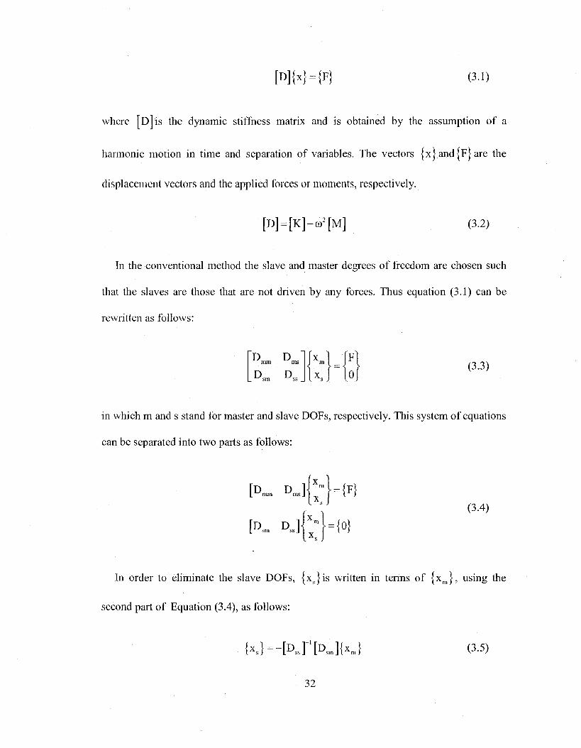
[D]{X} = {F} (3.1)
where [D]is the dynamic stiffness matrix and is obtained by the assumption of a
harmonic motion in time and separation of variables. The vectors |x}and{F]are the
displacement vectors and the applied forces or moments, respectively.
[D] = [K]-©2[M] (3.2)
In the conventional method the slave and master degrees of freedom are chosen such
that the slaves are those that are not driven by any forces. Thus equation (3.1) can be
rewritten as follows:
D D mm ms x"rC (33>
in which m and s stand for master and slave DOFs, respectively. This system of equations
can be separated into two parts as follows:
[ D - D"]fx"} = {F) (3.4)
[ D . D-]jx;[=!o}
In order to eliminate the slave DOFs, {xs}is written in terms of {xm}, using the
second part of Equation (3.4), as follows:
WHD.riDjK} (3.5)
32

Substituting this j x s | in the first part of Equation (3.4), the system of equations can be
written as follows:
> m m ] - [D m s ] [D s s r ' [D s m ] ]{x m h{F} (3.6)
Let F D ] = [Dmn,]-[Dms][Dss] [Dsm], for simplification, and equation (3.6) becomes:
M K H F } (3-7)
Richards and Leung [51] proved that the mass matrix is equal to the derivative of the
dynamic matrix with respect toco2, which can be seen from Equation (3.2). Consequently,
M = - - 7 ^ r [ D ] (3.8)
Differentiating |D*1 with respect toco2 will yield the condensed mass matrix as:
[M , ] = [ M - ] - [ D j [ D j , [ M j - [ M . ] [ D j 1 [ D j
+ [Dms][Dssr[Mss][Dss]
1[Dsm]
where — J [ D ] is obtained by differentiating the identity, [D] [D] = [l] .The reduced
stiffness matrix can be then obtained using the following relation:
[K*] = [D*] + CO2[M*] (3.10)
The reduced eigenvalue problem is then shown as follows:
33

r -co M'] = {F} (3.11)
This method requires the inverse of the dynamic matrix during the computation of the
natural frequencies.
3.2. Static condensation
The static condensation was first proposed by Guyan [30] and Irons [31]. This method
was later known as Guyan reduction or eigenvalue economization. The main idea in this
method is to eliminate the slave degrees of freedom in terms of the master DOFs. This
choice is mainly related to the distribution of energy. Thus for different modes different
selection of master and slave DOFs is required.
Similar to the exact dynamic condensation, the reduced eigenvalue problem will have
the same form as in Eq. (3.6). However, in this method a major assumption is used by
taking the inverse of [Dss]in Eq. (3.6) as follows:
[Dssr-[Kssr-co2[Kssr[Mss][Ksr (3.i2)
3.3. Boundary characteristic orthogonal vectors in the Rayleigh-Ritz
analysis
The Rayleigh-Ritz method was originally introduced as an extension of Rayleigh's
method and they were mainly used for continuous structures. However this method can
34

be applied to discrete systems also. Thus any discrete system can be reduced to a lower
number of degrees of freedom.
A more general method than that used in chapter 1 is followed to generate a set of
orthogonal vectors using the stiffness and mass matrices that satisfy all the requirements
of the flexibility as well as the boundary conditions of the structure under study, using a
procedure that was first introduced by Leger, Wilson and Clough [42].
3.3.1. Modified Gram-Schmidt method
The method of generating orthogonal vectors using Gram-Schmidt orthogonalization
is modified here based on the fact that some DOF may be dependent. The mass and
stiffness matrices can be rearranged to separate the slope from the deflection degrees of
freedom. The mass and stiffness matrices can be rewritten as follows:
[M]: [Mdd] [Mds] K ] [M„] W = [Kdd] [Kds]
Ksd] [K„] (3.13)
where the subscript "s" is for slopes and "d" is for deflections. As before, starting from a
uniform load the first vector is computed as the static deflection as shown in Eq. (1.9) .
Any other vector in the orthogonal vector set can be written as follows:
< P i = M (3-14)
Using Gram-Schmidt orthogonalization the second and the rest of the vectors are
obtained in the following two equations, respectively.
35

(p2=x(p,-b2(p, (3.15)
(P1+2=X(P1+1-bi+2(pi+1-c,+2(p, (3.16)
Taking only the deflection into account in Eq. (3.15) yields the deflection portion of the
second vector as:
(Pd.2=X(Pd,l-b2(Pd,l ( 3 - 1 7 )
Since the slopes are the derivatives of the deflections, we have
9s.2 = ~ h ~ = <Pd,i + x(Ps,i - b2(Ps,i ( 3 • 18) ox
Combining the slopes and deflections the vector (p2 can be written as follows:
-teHtehtei: Proceeding similarly, the higher members of the orthogonal set are obtained as
,M > « _ > - _ bwK. _C| > J ° (3.20) K i + 2 J K i + 1 J L<Ps,i+i J K d [<p„,i+ij
These modifications will help in getting a better admissible vector in the Rayleigh-
analysis resulting in a better convergence to the exact eigenvalues. However, this method
becomes quite complicated in case of complex structures.
36

3.3.2. Boundary characteristic orthogonal vectors by static deflection
In this method the calculation of static deflections due to a load distribution that is
proportional to the previous deflection vector is used. This method is also sensitive to the
first vector assumption. Knowing that the static deflection corresponds to zero frequency,
it is taken as the first eigenvector or mode shape which is the closest to zero. The static
deflections automatically satisfy the geometrical boundary conditions.
As before, starting from a vector similar to that of Eq. (1.9) the rest of the vectors are
obtained using the algorithm shown in Fig. 12 and 13. This algorithm consists of three
major computational steps:
• Computing the static deflection.
• Subtracting the contribution of the previous vectors for orthogonalization.
• Normalization.
Fig. 12 and Fig. 13 basically show the same information, however, in the later the
algorithm is shown in a block diagram highlighting the two loops. It should also be noted
that the stiffness matrix is a constant matrix and hence needs to be inverted once and
stored for use when needed. This step is shown also in Fig. 13 where the inverse of the
stiffness matrix i s stored as [ A ] = [ K ] .
37

1. {y,\r = [« ] " ' {»} whore|»|.ji I I .... if
(W'MW)2
2. Higher member {$,} (i=2,3,4,..., n=number of desired vector):
• Orthogonalization (j-l,2,3,...,i-l)
• Normalization:
Fig.12: Algorithm for the generation of orthogonal vectors.
38

Static deflection vector:
where, {s} = {\ I 1 l}'
w Normalization:
i )
(WMM)5
-•M=MM{4-,}
" / / = ^ "]M! -SEfch^it)
M={*}
Fig.13: Computation scheme for the generation of orthogonal vectors.
39

3.4. Comparison of different model reduction techniques
A close examination of both the static and the exact dynamic condensations will easily
show that both methods use a transformation from the complete model to the reduced
one. This transformation can easily be described in terms of the rearranged matrices using
slave and master DOFs. However, when both Gram-Schmidt method and the algorithm in
Fig. 13 are used the transformation lacks an explicit form in terms of the given matrices. It
should also be noted that extending the condensation methods for substructuring may be
difficult in some application due to the problem of matrix multiplication size.
Table 4: Transformation formulae for different methods.
Method Transformation formulae:
Static condensation
I x.iel vl\n;iimc Ciiiulcnsal:on
Orthogonal vectors in Rayleigh-Ritz
x„
r —
[-K„'][K„]
['] •['>..] I ' ' :
M=[*]M
k,}
1 Y ' t X in J
I V J is the matrix of orthogonal vectors
Using this method of formulation, the computation of the reduced order model
becomes very simple and it shows that all the listed methods are basically similar. The
general form of the reduced order model matrices can be written as the following matrix
product where [Tr] stands for the transformation matrix:
40

M = [T,rM[Tr] M = [Tr]T[M][Tr] (3.21)
3.5. Example structures
A set of example structures were investigated in order to compare different model
reduction methods. Both methods that use a set of orthogonal vectors are compared
together and the one using static deflection vectors is compared with both static and exact
dynamic condensations.
3.5.1. Cantilever beam
2 3 4 5 25
Fig. 14: Model of a cantilever beam.
A steel cantilever beam meshed into finite elements using one-dimensional beam
elements is investigated. The current section includes the results for all the listed methods
with different trials using different choices of master and slave DOFs. Eigenvalues are
computed and the mode shapes are plotted. The current model shown in Fig. 14 is
41

meshed into 25 elements resulting in 26 nodes and 50 DOFs since two DOFs are
constrained at the first node.
Table 5 shows the comparison of the reduced eigenvalues from both methods using
orthogonal vectors in the Rayleigh-Ritz method. The comparison shows that the modified
Gram-Schmidt method was capable to deal with the dependant DOFs resulting from the
slope degrees of freedom in the FEM model. Both methods have given good results for
up to half of the reduced order model, however, the second method has a better accuracy
and also gives a better approximation to the higher modes.
Table 5: Comparison between exact and reduced eigenvalues of both Modified Gram-Schmidt and Static load in the Rayleigh-Ritz method.
Modes
1 2
3 4 5 6 7 S 9 10
Modifl Scl
\alues
4177801~'" 261.8121 733.0768 1436.571 2375.352 3595.301 5123.112 9040.585 12773.29 59986.31
cd Gram-imidt
I-nor
(%) 0.0103 0.0027 0.0015 0.0O2
0.0227 1.3371 3.3719
36.9841 50.6313 466.044
Static dellections in the Raylei
value
41.7758 261.8049
733.0655 1436.5432 2374.8139 3547.8678 4959.5926 6791.0651 11007.8886 77951.9551
gh-Rit/. Frror
0 0 0 0 0 0
0.0725 2.N9i)|
29.8124 635.571
Fxact
41.7758 261.8049
733.0655 1436.54^2 2374.8139 3547.8632 4956.0014 6599.733 8479.8412 10597.4653
42
0 0.8 0.9 0.3 0.4 0.5 0.6 0.7 Global coordinate
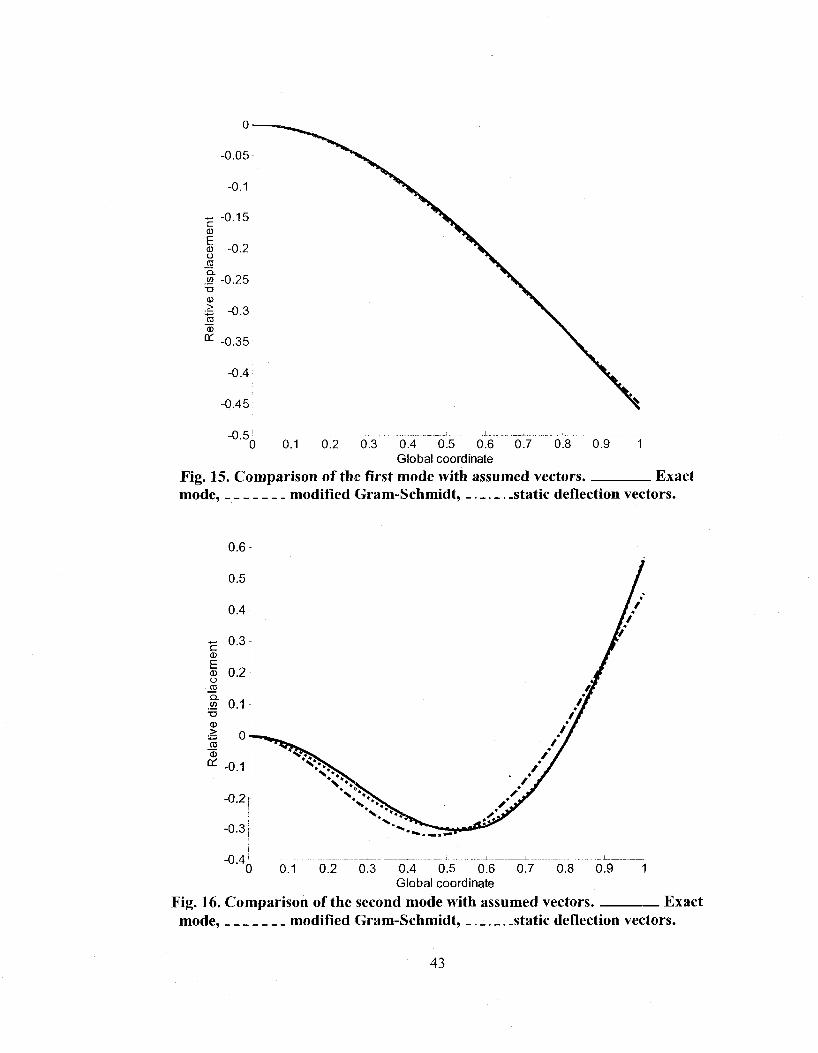
Fig. 15. Comparison of the first mode with assumed vectors. Exact mode, modified Gram-Schmidt, .static deflection vectors.
0.2 0.3 0.4 0.5 0.6 0.7 Global coordinate
0.8 0.9
Fig. 16. Comparison of the second mode with assumed vectors. Exact mode, modified Gram-Schmidt, _. _ static deflection vectors.
43

0.7
iace
men
t di
sp!
Rel
ativ
e
Fig. 17. mode,
0.6:
0.5:
0.4!
0.3
0.2'
0.1
-0.1
-0.2
-0.3-0 (
Compar
0.1 0.2 0.3 0.4 0.5 0.6 0.7 0.8 0.9 Global coordinate
Comparison of the third mode with assumed vectors. Exact modified Gram-Schmidt, static deflection vectors.
0.8
0.2 0.3 0.4 0.5 0.6 Global coordinate
Fig. 18. Comparison of the fourth mode with assumed vectors. Exact mode, modified Gram-Schmidt, static deflection vectors.
44

0.4
-0.8
- 1 '- - ! '••
0 0.1 0.2 0.3 0.4 0.5 0.6 0.7 0.8 0.9 1 Fig.19. Comparison of the fifth mode with assumed vectors. Exact mode, static deflection vectors, modified Gram-Schmidt.
Fig. 15 to 19 show the comparison between the exact eigenvectors calculated from
FEM and the assumed vectors from both methods. The results show that the vectors
resulting from modified Gram-Schmidt method are closer to the exact vectors than that of
the deflection due to static load. However, the eigenvalues of the latter are closer to the
exact ones than the former. This can be justified by the fact that the static deflection
vectors satisfy the flexibility restriction of the system since the inverse of the stiffness
matrix is used to calculate all the vectors which will ensure that the vectors satisfy all the
boundary conditions. It should be noted that the plots of the vectors are based on the
deflection only.
45

The same cantilever beam is also reduced using static and dynamic condensation
methods. Different choices of the master degrees of freedom are taken and for every case
the results are presented and discussed. First, the master DOFs are chosen to be on node
22 to 26 of the model shown in Fig. 14. This resulted in a reduction to a (10x10) reduced
order model. Further, the model was reduced by the choice of different master DOF
where they have been chosen along the span of the beam, namely, nodes 1, 4, 9, 13... 49.
Table 6 shows a comparison between the reduced order model natural frequencies
using the three different methods. It should be noted that the selection of the master DOF
has resulted in the loss of some modes. The numbers in parenthesis gives the equivalent
mode of the complete structure. As shown, the exact dynamic condensation will give
always very close results, however, this method is an iterative method that needs to
converge toward the exact solution at each frequency of interest. Hence it makes the
process computationally demanding. Moreover it is affected by the choice of the master
DOFs. The static condensation method shows good results at the first frequency which is
closer to 0 or the static condition. The use of orthogonal vectors in the Rayleigh-Ritz
method gives good results without the need to choose either the master or slave DOFs.
This method will also guarantee the sequence of modes, in other words the resulting
reduced modes will always be in an ascending sequence due to the nature of this method
that applies the Rayleigh-Ritz analysis. Moreover, the error in the higher modes can
easily be reduced by using a larger number of vectors if desired.
46

Table 6: Comparison between the reduced eigenvalues of different reduction methods.
Mode
1 2 3 4 5 6 7 8 9 10
Dynamic condt
Values (Hz.)
41.7758 261.8049 6599.733 32278.326 66693.639 113667.0506 165892.2678 236813.1874 322578.9028 444651.1542
jnsation.
Error (%) (1)0 (2) 0 (8)0 (17)0 (24) 0 (30) 0 (35)0 (40) 0 (45) 0 (50)0
Static condensation.
Value (Hz.)
41.8224 315.3932 2896.8566 12255.104 30907.010 58863.057 107700.19 171984.56 271107.71 442445.70
Krror (%)
(1) 0.11 (2) 20.4688
295.170 753.0968 1201.4498 1559.1129 2073.1268 2505.9322 3097.0848 4075.0144
Static load vectors in Rayleigh-Ritz.
Values (Hz.)
41.7758 261.804 733.065 1436.54 2374.81 3547.86 4959.59 6791.06 11007.8 77951.9
Krror (%)
0 0 0 0 0 0
0.0725 2.8991
29.8124 635.571
Table 7 shows the natural frequencies of the cantilever beam using a reduced model
and with a better choice of master DOF. It is clearly shown that the natural frequencies,
calculated from dynamic condensation, show a better result always with negligible error.
However, the static condensation gives poor results. This is because this method searches
for the static deflection state at which the beam has its maximum energy located at the
master DOFs.
47

Table 7: Comparison between the reduced eigenvalues of different reduction methods.
Dynamic condensation. Static condensation. Mode
Static load vectors in Rayleigh-Ritz.
Values (Hz.) Error (%)
Value (Hz.) Error (%) Values (Hz.)
Error (%)
1 2 3 4
5
6 7 8 9 10
41.7758
261.8049
733.0655
1436.5432
2374.8139
3547.8632
4956.0014
6599.733
8479.8412
55673.9094
(1)0
(2)0
(3)0
(4) 0
(5)0
(6) 0
(7)0
(8)0
(9)0
(22) 0
2508.3685
6359.0402
7739.6378
9349.6256
13754.140
16327.307
20640.528
22496.269
24703.337
31415.925
(5) 5.6238
(8) 3.6470
(9) 8.7290
(11)6.1753
(12)4.9846
(14)3.9215
(14)4.7167
(15)0.4837
(17)2.6718
41.7758
261.804
733.065
1436.54
2374.81
3547.86
4959.59
6791.06
11007.8
77951.9
0 0 0 0
0
0 0.0725
2.8991
29.8124
635.571
3.5.2. Simply supported beam
The case of a simply supported beam is studied using both the dynamic condensation
and the orthogonal vectors in the Rayleigh-Ritz method. The results, shown in Table 8,
highlight the sensitivity of the dynamic condensation on the correct choice of the master
degrees of freedom. In this case also the same number as well as the same choice of
degrees of freedom as in the second case in the cantilever beam have been used. This
choice gave good results in the case of cantilever beams, however, it was not capable to
do so in the case of simply supported beams.
Moreover, the error in the sixth natural frequency using the orthogonal vectors came
to be higher than that of the fifth. This should not happen usually in the Rayleigh-Ritz
method, however, this might have been due to some poorly scaled vector, which includes
very large numbers compared to the others. A very good study about the effect of
48

assumed mode components on the results of Rayleigh-Ritz analysis was carried out by
Bhat [52].
Table 8: Comparison of natural frequencies of SS beam.
Mode
1 2 3 4 5 6 7 8 9 10
Dynamic condensation.
Values (Hz.)
117.2666 469.0674 1876.3471 9508.9999
108571.4592 293539.6389 310537.3321 326820.6804 341733.1594 354516.9925
Equivalent mode
1 2 4 9
29 43 44 45 46 47
Static load \ Rayleigh
Values (Hz.)
117.2666 469.0674 1055.4135 1876.3471 2931.9771 4222.536 6131.0667 76I0.41)35 13731.573 184179.71
'ectors in -Ritz.
Error (%)
0 0 0 0 0 0
6.657 1.335
44.4061 1468.0
3.5.3. Clamped-clamped beam
Clamped-clamped beams are also studied using the modified Gram-Schmidt,
orthogonal vectors generated as static deflection and the dynamic condensation. Fig. 20-
22 show the comparison between the exact mode shapes of the structure with the
assumed vectors for the Rayleigh-Ritz analysis. Again both methods show good
resemblance to the exact mode shapes, however, in terms of results, the second method
has better accuracy. Also it should be noted that the modified Gram-Schmidt method
would be somewhat difficult in the case of two or three dimensional problems since it
requires the coordinates of the nodes.
49

0.4
0.35
0.3 -*—i c CD
E 0.25' 0 o IS .§" 0.2^ 73 CD > 'm 0.15 CD
a: 0.1;
0.05 r
0 0.1 0.2 0.3 0.4 0.5 0.6 0.7 0.8 0.9 1 Global coordinate
Fig. 20. Comparison of the first exact mode with assumed vectors Exact mode, modified Gram-Schmidt, static deflection vectors.
•»--•»
0 0.1 0.2 0.3 0.4 0.5 0.6 0.7 0.8 0.9 Global coordinate
Fig. 21. Comparison of the third exact mode with assumed vectors. Exact mode, modified Gram-Schmidt, static deflection vectors.
50
0.4
, •
c CD E CD O _TO Q. c/3 T3 CD > 'CD CD CC
0.3 / / \ * 9 »
* / •
* / * * # * i 0.2 / /
* m
** / * / 0 1 / /
* # ** / * / 0 * - 7
\ -0.1 \
* \ *
-0.2: \ \ * \ • »
-0.3: \ /
- 0 . 4 - • ' •_ -
r. i \
• * . • '
0 0.1 0.2 0.3 0.4 0.5 0.6 0.7 0.8 0.9 1 Global coordinate
Fig. 22. Comparison of the fifth mode with assumed vectors Exact mode, modified Gram-Schmidt, _. static deflection vectors.
Table 9: Comparison between the reduced natural frequencies of different methods for CC beam.
Mode
1 2
3 4 5 6 7 X 9 10
Dynnmic condi
Values (11/.)
'"""205.8303 732.775X 1436.5609
2374.X 141 3547.X6X 4956.0166 6599.7745 S479.940N 55734.6248 167160.9X2X
jnsaiion.
Trior
Co) ( D O (2)0
(3) 0 H ) 0
(5) 0 ((••) 0
(7)0 (X) 0
(21)0 (34)0
Modified ( iram-Sehmidt.
Value (11/.)
277.1925 744.574X 1449.6511 23X9.7234 3565.5399 49X2.0496 6964.5501 91X1.6729
16933.2757 22612.2036
iTrurCn)
4.2742 1.6102 0.9112 0.627X 0.49X 1 0.5253 5.5271 X.2752 59.7X2X 74.5493
Sialic loai in Raylei:
Values
265.8303 732.775X
1436.560 2374.814 547.X68 4956.176 6674.132 XX27.7I7 16682.32 277324.5
1 \ectors yji-Ritz.
1 irror
() 0 0 0 0 0.0032 1.1267 4.1012 57.4148 2040.73
51

Table 9 shows the comparison between the eigenvalues computed using different
reduction methods for the clamped-clamped beam. The exact dynamic condensation will
not show a significant error, however, it causes a loss of some modes with a poor choice
of master DOFs. The modified Gram-Schmidt method shows acceptable results,
however, it is computationally inconvenient in case of complex geometry. Finally the
orthogonal vectors generated by the static deflection algorithm shows good results with a
simple procedure. It should also be noted that both the exact dynamic and the static
condensations require a rearrangement of the FEM matrices. That also may be
computationally inconvenient. Moreover, the iterative nature of the solution of dynamic
condensation requires a starting frequency, and may create the problem of repeated
frequencies.
In this chapter, Gram Schmidt method was modified to deal with dependent degrees of
freedom. Moreover, a new method of generation of the vectors is proposed and the
formulation and the algorithm are presented. Static and dynamic condensation methods
are presented and discussed. The latter two methods and the newly proposed ones are
compared using FEM models for different beams. In the next chapter the method that
employs the vectors generated as static deflections is applied to different case studies.
52

Chapter 4
Applications of the model reduction using orthogonal
vectors set in the Rayleigh-Ritz method.
4.1. Introduction
In chapter 3, the newly proposed method of model reduction by boundary
characteristic orthogonal vectors was investigated and the results were compared with
earlier studies. In this chapter the application of this method on different case studies will
be carried out. First a model of a vehicle system with components having distributed
mass and elasticity as well as attached discrete degrees of freedoms will be studied, and
then a coiled heat exchanger meshed in ANSYS.
In the first case the main interest is to find the mode shapes of the vehicle model and
its harmonic response. The vehicle is modeled as a flexible beam with two spring damper
mass systems attached to it. The vehicle itself is also elastically connected to the ground
through which it receives some disturbances. It should be noted that the damping
coefficients for the discrete dampers are taken into account, however, no structural
damping is considered for the chassis beam.
The second case is an investigation to obtain the natural frequencies of a coiled heat
exchanger proposed by Kumar, et al. [56]. This model is meshed into three dimensional
elements including 6 DOF at each node. The resulting matrices are reduced and the
53

eigenvalue results are compared with those of the complete FEM model of the system.
The mass of the fluid contained in a beam element is simply added to the mass of the
beam element itself, however, the flow effect of the fluid are not considered.
4.2. Harmonic analysis of vehicle reduced order model
In this section, a vehicle hybrid model consisting of a combination of discrete and
continuous subsystems is analyzed. The discrete subsystems represent the human body
and the engine as two masses elastically connected to the chassis. The continuous
subsystem represents the chassis of the vehicle that is modeled as a beam. The FEM
modeling of this structure is done using a MATLAB program. The constraints applied on
the system represent the wheel contacts. Fig. 23 shows the model of the vehicle used for
the study. The two attached masses are constrained to move vertically.
Fig. 23. Vehicle body model with attached spring mass systems.
54

The finite element model of the system shown in the above figure was constructed
using one dimensional bending beam elements and lumped masses elastically attached to
the chassis for the discrete blocks. Hence the attached masses constitute two additional
nodes. The model is made of a total of 125 nodes where only the last 4 correspond to the
rear wheel, front wheel, engine and driver, respectively. The resultant FEM model yields
atotalof246DOFs.
Those DOF are precisely formed of 121 translational and rotational degrees of
freedom along the beam, and 4 translational degrees of freedom for the four connected
spring mass systems. The length of the elements is taken to be 0.1 m. Hence the engine is
connected at the node number 61 and the driver is connected at node 111. Nodes 122 and
123, corresponding to the wheels, are assumed to keep contact with the ground. This
assumption is equivalent of replacing the nodes with two pins. The locations of the most
important nodes are given in Fig. 24.
Z4(t)
w(x,t)
Fig. 24. Node location of FEM model.
55

The parameters used in the study are given in Table 10. These Parameters correspond
to a city bus and have been taken from [53-55], and those that are not found in [53-55]
have been estimated.
Table 10: Numerical parameters.
Parameter
L X\
*2
*3
X4
Kir
k,/ kd
ke
Csr
<-'sf
Cd
Ce
md
me
pA EI
Value
12 3 1 9 11
280 240
10500 140 4 7
830 800 70
3600 1000
1
Unit
in
m in
m m
kN/m kN/m N/ra kN/m
kN.s/m kN.s/m N.s/m N.s/m
kg kg
kg/m MNm2
The reduced model is obtained using ten orthogonal vectors, resulting in (10x10)
eigenvalue problem. The eigenvalues of the reduced model are calculated and compared
with the exact ones in Table 11. The computed values show a good agreement with those
for the complete system model. The eigenvalues for the reduced 10 DOF model agree
with those of the complete model with an accuracy up to the 4th decimal place until the 6th
56

natural frequency and then slowly start increasing for the higher ones as expected. The
last two values are far higher than those for the complete model.
Table 11: Comparison of exact and reduced natural frequencies.
Mode
1 2 3 4 5 6 7 S 9 10
0.18
0.16
0.14
0.12
o 0.1 NJ • D N 0.08
0.06
0.04
0.02
0
- '- -
•? •
;
z
i
•
* ** • a
Natural Frequencies
Reduced 0.7075
Exact 0.7075
0.8906 0.8906 1.1888 1.1888 1.9039 1.9039 2.5674 2.5674 6.9303 6.9303 13 4438 13.4434 lUmh 22.098 46 6682 33.01 11 127.3379 46.1088
0.18
0.16?
0.14
; 0.12! : i m m
*
m* m*
« • • •
• • mm
• • • • • •
o 0.1 NJ T3 N 0.08
0.06
0.04 • • /
« • \ g
.»' : 0.02 [ /
* * • » > • • • • • • 0
Error
(%)
0 0 0 0 0 0
0.003 0.0027
41.3715 176.1685
' V J v^y
, , : ,
-
1
\ ~ — -0 0.5 1 1.5 2 2.5 3 3.5 4
Frequency (Hz.) 0 0.5 1 1.5 2 2.5 3 3.5 4
Frequency (Hz.).
Fig. 25. Transmissibility plots of the exact and reduced models. model, reduced model.
Exact
57
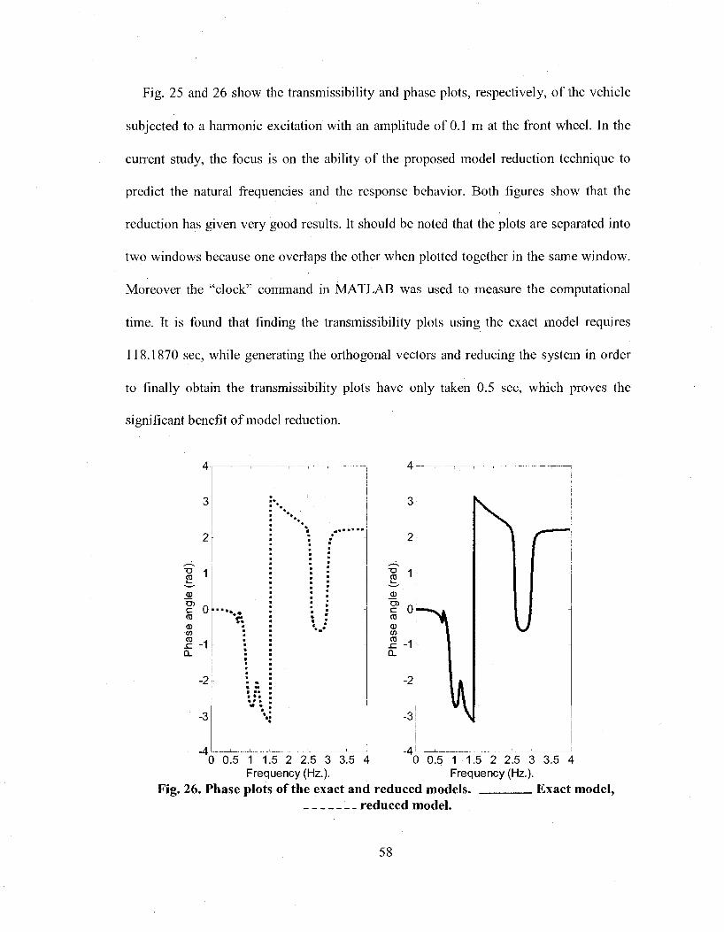
Fig. 25 and 26 show the transmissibility and phase plots, respectively, of the vehicle
subjected to a harmonic excitation with an amplitude of 0.1 m at the front wheel. In the
current study, the focus is on the ability of the proposed model reduction technique to
predict the natural frequencies and the response behavior. Both figures show that the
reduction has given very good results. It should be noted that the plots are separated into
two windows because one overlaps the other when plotted together in the same window.
Moreover the "clock" command in MATLAB was used to measure the computational
time. It is found that finding the transmissibility plots using the exact model requires
118.1870 sec, while generating the orthogonal vectors and reducing the system in order
to finally obtain the transmissibility plots have only taken 0.5 sec, which proves the
significant benefit of model reduction.
E,
D> C OJ
<D 0) ns -1
-3
4r
r.
0 0.5 1 1.5 2 2.5 3 3.5 4 0 0.5 1 1.5 2 2.5 3 3.5 4 Frequency (Hz.). Frequency (Hz.).
Fig. 26. Phase plots of the exact and reduced models. Exact model, reduced model.
58

3.5 3.5
2.5
o N •5 N
1.5
0.5 0.5 "0 0.5 1 1.5 2 2.5 3 3.5 4 " 0 0.5 1 1.5 2 2,5.3 3.5 4
Frequency (Hz.). Frequency (Hz.).
Fig. 27. Transmissibility plots of exact and reduced models Exact model, reduced model.
3.5
2.5
o N -6 N
1.5
0.5
3.5 f
f\
2.5
o N 2 X5 N
1.5
0.5 0 0.5 1 1.5 2 2.5 3 3.5 4
Frequency (Hz.).
Fig. 28. Transmissibility plots of exact and reduced models. model, reduced model.
0 0.5 1 1.5 2 2.5 3 3.5 4 Frequency (Hz.).
Exact
59

Fig. 27 and 28 show the transmissibility plots due to a harmonic excitation to the rear
wheel and to both the wheels, respectively. Those plots also show the capability of the
reduced order model to approximate the response to a harmonic excitation with a great
saving in the computational effort.
4.3. Model reduction of a fluid filled pipe
The proposed model reduction technique is applied on a three dimensional structure of
a coiled pipe heat exchanger filled with water. The model is used to simulate the
vibration behavior of the coiled heat exchanger proposed in [56]. The original structure is
made of 8 identical banks, one of which is shown in Fig. 29.
Fig. 29. Sketch of one bank of the coiled heat exchanger.
60

4.3.1. Modeling using FEM
The modeling of the structure is done in two parts. First the structure is plotted in
MATLAB, and the coordinates are transferred to ANSYS where the model is created and
meshed. The resulting matrices are taken from ANSYS to MATLAB in order to perform
necessary matrix operations for the reduction.
Initially, the coiled heat exchanger is represented by a total of four 3D curves. Those
curves are made from parametric equations containing two terms as trigonometric
functions while the last is linear along a direction. The general form of those equations
are shown below,
x = axt
y = a2sm(t) (4.1)
z = at cos(/)
The four exact functions used in this case are shown in Table 12. As seen, the
equations are linear either along x or y which coincides with the axis of the circular coil.
And the minus sign that multiplies t in some equations is appearing because the structure
is going backward at the definite bend.
Fig. 30 shows the representation of the bank shown in Fig. 29, using the parametric
equations presented in Table 12.
61
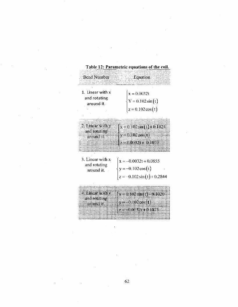
Table 12: Parametric equations of the coil.
Bend Number Equation
1. Linear with x
and rotating
around it.
x = 0.0032t
Y = 0.102sin(t)
z = 0.102cos(t)
2. Linear with y and rotating
around i l .
x 0.l02sin(t) 1-0.1N24
y:-().K)2eos(l)
/ = 0.00321+ 0.1070
3. Linear with x and rotating around it.
x = -0.0032t +0.0855
y = -0.102cos(t)
z = -0.102 sin (t) + 0.2844
4. Linear with y and rotating
around it.
[x =0.102 s in( t ) -0.1()20
> = -0 . l02cos( t )
/ =-().0032t-i-0.1X75
62

0.5
0.4
0.3
~ 0-2
N 0.1
0
-0.1 / 0.15 / - 0.1
X 0.05 -0.2 > / ' ' JD„ -0.4 ~~ -0-05
-°-3 -0.2 .0.1 - '-- /"-:0.1 0 °-1 02 0r-o.?-15 Y(m).
X(m). Fig. 30. The simulation of the coil bank by a 3D curve.
Fig. 31 shows the simulation of the coil bank using the set of parametric equations
presented in Table 12. The smoothness of this curve is ensured by taking a small
increment oft. While in case of Fig. 31, the increment is taken as y. and the resulting
components of each point are stored since those will form the geometry input to AN SYS.
As shown in Fig. 31, as well, the chosen increment does not result in the distortion of the
geometry. The operated mesh in MATLAB has resulted, in a total of 128 elements and
129 nodes, resulting in 774 DOFs with 6 DOFs at each node. The geometry and
properties of the coil are shown in Table 13.
63

0.15-
0.1
0.05
^ ° N -0 05
-0.1
-0.15
-0-2.
8.o
6.08 „ „ < : . n 1 f i -o.i
fro* 6 o e . o - - - ° 0 5 ^ ^ > - . . - V ' ~ 0.05^-1 ° 1 5
: o , -0-05
09 -0.2 " 0 / l 5
X(m). Y (m ) -
Fig. 31. Exact vs. meshed models.
Table 13: Geometry and parameters of the coil. Outer diameter Wall thickness Radius of curvature of the coil Pitch of the coil Modulus of elasticity of pipe Material Shear modulus of pipe material Mass per unit length of the pipe Mass per unit length of the fluid
4.3.2. Reduction of the model
The model is assumed to be supported at nodes, 65, 73, 81, 89 and 97, where the coil
is constrained in all directions. The positions of those nodes are shown in Fig. 32.
12.7 1.2 102 20 iy."? 7S 0.34SI 0.0833
mm mm mm mm Mpa Mpa kgin Kg/m
64

• • • • •
0.2
0
0 0.1 o.2 o.3 " ° 2 Y ( m ) -
X (m). Fig. 32. Support locations.
Two cases of reduction are performed; one using 10 orthogonal vectors and the second
using 20 of them. The resulting natural frequencies are compared with the complete
model solution.
Table 14: Eigenvalue of reduced (10 natural frequencies) and complete model. odes
I -j
4 5 (> 7 8 o K)
Reduced Model
(Hz.) o.oi is 3.2602
3.4524
6.2023
6.0675
0.0033
12.0002
16.8803 25.3SOS
47.8071
l;LM(ll/.)
0.01 18
3.2692
3.4524
6.2023
6.0(>75
0.0012
I0.0I5X 1 1.0080
16.4053
10.2100
l-:rmr(%
0 0 0 0 0
0.021
20.80
40.76
53.87
148.86
0.5
0.4
0.3
^ 0.2
N 0.1
0
-0.1
-0.2 -0.4 -0.3 -0.2
65

Table 15: Eigenvalue of reduced (20 natural frequencies) and complete model. [odes
1 2 3 4 5 6 7 8 9 10 11 12 13 14 15 16 17 IS 19 20
Reduced Model (Hz.) 0.9118 3.2692 3.4524 6.2023 6.9675 9.9012 10.0158 11.9989 16.4953 19.2100 20.6708 22.8776 24.9467 27.9811 30.3406 37.4754 43.9935 56.2358 82.1543 437.6680
F E M (Hz.)
0.9118 3.2692 3.4524 6.2023 6.9675 9.9012 10.0158 11.9989 16.4953 19.2100 20.6704 22.5287 22.9538 25.2499 28.8345 30.0403 31.6851 32.7026 35.3791 37.6601
Error (%)
0 0 0 0 0 0 0 0 0 0
0.0018 1.5487 8.6819 10.8164 5.2234 24.7504 38.8461 71.961 132.2116 1062.1524
Table 14 and Table 15 show the reduced natural frequencies and their comparison
with those from the complete FEM model. It is shown in both cases that this method is
capable of approximating around half of the reduced order model results with negligible
error.
66

60
o UJ
10th natural frequency 111th natural frequency 112th natural frequency 113th natural frequency
15 16 17 18 19 20 21 22 23 24 Number of employed vectors.
Fig. 33. Convergence history of 10th, 11th, 12th, and 13th modes.
Fig. 33 shows the convergence history of 10th to 13th modes versus the number of
employed vectors. As seen before in Table 14 and Table 15, the higher order of the
reduced model eigenvalues have poor values with large errors. This convergence history
t i l
plot shows that the 13 natural frequency converges toward that of the complete model
when a total of 22 vectors are employed. Hence the number of employed vectors should
be larger than the number of desired modes to secure a better convergence at the higher
modes of the reduced model.
67

200
180
160
140
120
§ 1 0 0 =
1st natural frequency 2nd natural frequency
i / ^ 3rd natural frequency • • 4 t h natural frequency
UJ 80
60
401 j
20;
oL 1 1 2 3 4 5 6 7 8
Number of employed vectors. Fig. 34. Convergence history of 1st, 2nd, 3rd and 4th modes.
Fig. 34 shows the convergence history of the 1st to 4th modes. When only one vector is
used, one bar can be noticed which represents the error at the 1st natural frequency. On
the other hand when two vectors are used, it should be noted that two bars corresponding
to the error at the 1st and the 2nd natural frequencies must be represented. However only
the latter is shown since the former have already converged to zero. When the number of
used vectors reaches 4 the number of bars will remain 4 afterward, since the convergence
of only the firt four natural frequencies is studied. Note that when 7 vectors are used in
the study the error is almost zero in all the 4 modes.
68

In this chapter the proposed model reduction method is applied on two models of a
vehicle and a coiled pipe, respectively. The orthogonal vectors are the physical static
deflection due to a load distibution. However, a set of vectors that are calculated in a
similar manner can be used to solve any system of equations. In these cases, the vectors
will be a generalized coordinate vector. In the coming chapter, the Rayleigh-Ritz method
with orthogonal polynomial functions in two dimensions are used to solve problem of an
elliptical plate. The resulting generalized stiffness and mass matrices are reduced using
the newly proposed algorithm.
69

Chapter 5
Using independent vectors for the reduction of
generalized eigenvalue problem
The boundary characteristic orthogonal vectors were calculated in previous chapters as
the static defflections due to loads proportional to the preceding assumed deflection
shapes. In this chapter the coeficients of the assumed functions are considered as
generalized coordinates and the reduction is done on the number of the new generalized
coordinates used in the reduced model. The case of an elliptical plate is studied using two
dimensional orthogonal polynomials in the Rayleigh-Ritz method.
A systematic method of generating the admissible functions of arbitrary clamped
plates with different shapes is presented. The method of orthogonalization is similar to
that proposed by Staib [29].
5.1. The Rayleigh-Ritz method for plate vibrations
As mentioned earlier the Rayleigh-Ritz method requires the expressions of the energy.
For the plate case the kinetic and strain energy expressions are shown in Eq. (5.1) and
(5.2), respectively. Note that, w(x, y)is replaced byw and a, b and h are the dimensions
of the plate in x, y and z directions, respectively, and D - &" / , , \ is the flexural
F / l 2 ( l - v 2 )
rigidity. The boundaries of the integrals are defined by the geometry of the plate.
70
^max =-ph®2\\w2dxdy (5.1)
U„ Mi d2w + <r
1 fwY
v W J +
2v fd2w^
ydx J 'dV
By + 2 ( l - v )
( d2w V
\uy J ydxdy j
(5.2)
dxdy
The deflection is expressed as a sum of assumed mode shapes cpm (x, y) as shown below:
w (-^j ;)=E^(x^)^ (5.3)
Introducing the non dimensional parameters, a = —, £ = — , tj = — in Eq. (5.3): b a b
w(£?)=£>«(£?)** (5.4)
Substituting Eq.(5.4) in Eqs. (5.1) and (5.2) results in the following two equations,
respectively:
T^^phabm'Ww'dtdT] (5.5)
U = i / ) 4 f (I 2 a"
'aV2
^ + tf
^82w^
\drr , +
Iva1
K^2 j + 2 ( l - v / ) a 2
Kd£drj j
(5.6)
d<^drj
71
Using the stationarity condition of the Rayleigh's quotient results in the following
eigenvalue problem:
d'U dT ™x__ ^ 2 _=»><_ = () forn = ^2,...,N. (5.7)
where, N is the number of assumed mode shapes and X1 = 7 2 4
phco a
D
is the non-
dimensional eigenvalue. Eq. (5.7) can be rewritten as a matrix eigenvalue problem as
follows:
EI][X-*2<k=° (5.8)
where,
*.=h d^di] + a4 j a>, d£,drj
+ 2va2\\
V v ^ 2 y v 5>7 2y +
d <Pj 2 d?
2 „ \ 5 > ,
d?;2
+ 2(l-vK fjf-^
d^drj
d^di],
Mn^\\(Pi(Pjd^drl
Eq. (5.8) can also be written in (NxN)generalized matrix form, f in -/I2 |M 1 = 0. This
form is that which will be reduced using the orthogonal vectors matrix transformation.
72

5.2. Assumed deflection shapes
The conditions at a clamped support are that the deflection and slope are zero. The
first deflection shape is assumed as the simplest function that satisfies the geometrical
boundary conditions. These conditions at an arbitrary support F(^,rj) are shown below:
<P\ F{£,V) d<P\
d% = 0, 8<P\
n?*) drj = 0
nz>*) (5.9)
F i ( x . h )
F 2 (x ,h)
x Fig. 35. General plot of a rectangular plate with line supports.
A function that can satisfy the conditions of Eq. (5.9) can be found as:
<p1(i7,t) = F2(t,Tj) (5.10)
73

The fact that this shape function satisfies the listed condition can easily be proved by
differentiating in both directions. In case of multiple supports as in Fig. 35 the first shape
function can be taken in the following form:
?,(*,£) = F,2 ( £ ? ) / ? ( £ 7 ) (5.11)
The orthogonality condition used for the orthogonalization procedure can be defined
in view of the nature of the problem. For example the case of nonhomogonous structures
can be studied using a weight function in orthogonalization. In the present case the plate
is uniform and the orthogonality condition is taken as follows:
\\<pi<pjdZdr, = 0 (5.12)
In order generate the rest of the functions, a linear independent basis O of a vector
space V is created by multiplying the first functions by<^rr/s, following the sequence
shown in Fig. 36.
74

/Pi \
V(P\ J<P\ \ /
/ \ / \ / ' \ /
T T
Fig. 36. Scheme of generating the linear independent basis.
The inner product in the space V is defined as follows:
(<PPPJ ) = \ j<Pi<Pj d^dt] (5.13)
The boundaries of the integration are defined by the plate in study. The inner product
matrix representation of the basis <1> is obtained as follows:
2̂ = J J W . ^ 7 7 (5-14)
where (p. and ^.are, respectively, the z'Aand j"' element of^>, and 2 .̂ are the elements of
[/?]. It can be easily seen that [#]is symmetric. Eq. (5.3) can be rewritten in the
following form:
^ = ! > , < * = K k 4 (5-15)
75

where qx „, is the Ocoordinate representation of Wx. Thus, W2 can be written as follows:
^=KV*} (5.16)
Using the two previous equations, the inner product of two arbitrary shape functions
can be obtained as follows:
b b . r<l • Y " A
. i=l J \ i=l J
(5.17)
Rearranging Eq. (5.17) yields:
fbb \
w = S I i Um i = I I 4 ( ^ ) i (5-18) '=1 >1 V a a J 1=1 7=1
It is easy to see that Eq. (5.18) can be written as follows:
{Wx\W2) = [q^[B}[q2^~\ (5.19)
Knowing that any space may have many ordered basis, the goal is to find another
orthogonal ordered basis /3. Let qx p and q2 fi be the representative /? of the any deflection
function. Defining the relation between the coordinate representation of <E>and/? to be as
follows:
4a> = [^f qp (5.20)
Thus,
76

v=M\/? (5-21)
42,* = [A]'hf (5-22)
Using Eq. (5.21) and Eq. (5.22), Eq. (5.19) can be written as follows:
{W]W2) = ([Af qUi J [B]([A]T q2tfi) = q[p {[A][B][A^)q\_p = q{p ([D])qT2J (5.23)
From the previous equation we can say that if the matrix [D] is diagonal, then the basis
/?is an orthogonal basis. From linear algebra, the change of basis matrix is equal to the
inverse of the transpose of the change of coordinate matrix. Thus, knowing that the
transformation matrix in this case is [Af as shown in equation (5.20), the two ordered
basis are related by the following equation:
(D: (14)' P (5.24)
hence,
P = [A]Q> (5.25)
A process, similar to that of finding the inverse of a matrix, is used in order to find [.4]
matrix. The Identity matrix is augmented to B matrix. The matrix B is transformed to an
upper triangular matrix by a set of row operations, while the added identity matrix will be
77

converted to a lower triangular matrix. The proof that matrix [A] satisfies the desired
conditions is found in appendix-A.
5.3. Numerical result for elliptical plate
The case of elliptical plate is studied and the resulting stiffness and mass matrices are
reduced using the newly proposed method in chapter 4. In this case a total of 25 functions
were used and the generalized stiffness and mass matrices are of the size (27x27). These
matrices are reduced to a (10x10) different generalized matrices.
Fig. 37 shows the assumed mode shapes obtained from the process explained in
previous section. As shown, those plots can be arranged in four different groups:
• Symmetric about x-axis and y-axis (SS): 1, 4, 6, 11, 13, 15...
• Symmetric about x-axis and anti-symmetric about y-axis (SA): 3, 8, 10...
• Anti-symmetric about x-axis and symmetric about y-axis (AS): 2, 7, 9, 16...
• Anti-symmetric about x-axis and y-axis (AA): 5, 12, 14...
78

0 0.5 1 0 0.5 1 0 0.5 1 0 0.5 1
0 0.5 1 0 0.5 1 0 0.5 1 0 0.5 1
Fig. 37. Assumed mode shapes for elliptical and circular plates.
The plots shown in Fig. 37 are used for all elliptical plates since in the current
formulation due to the introduction of the non-dimensional parameters all the ellipses are
mapped on a circle. The ellipse is defined by the ratio of the major to minor axis, a = —. b
Fig. 38 shows the mode shapes of circular plates, fora = l. It is also seen that the
resulting modes can be distinguished by the same criteria used to group the assumed
ones. However, in the present case the (SA) and (AS) modes are merged to form one
group. This is justified by the rotation of the axis of symmetry in those modes. Thus, if
the plots are rotated to align the axis it can be seen that they are the same.
79

0 0.5 1 0 0.5 1
of circular plates a = 1.
80

As shown in Fig. 39 the elliptical plates are grouped into the four categories as well,
however, the rotation of the axis does not occur in this case since the plots are for
elliptical plates and, unlike the circular case, the axis length varies with the angle.
Table 16: Comparison of the eigenvalues of reduced and full models of circular plates a = 1.
Modes
1 2
4 5 6 7 8 9 10
Eigenvalues Reduced 40.8633 85.0419 139.5849 140.6128 159.4812 204.8935 272,418
319.0803 444.9232 649.3014
Complete 40.8633 85.0419 139.5107 139.6302 159.2964 204.8364 204.8364 245.6296 280.2286 282.6517
Error (%)
0 0
0.0532 0.7037 0.116
0.0279 32.993 29.903 58.7715 129.7179
Table 17: Comparison of the eigenvalues of reduced and full model of elliptical plates a = 2.
Modes
1 2 3 4 5 6 7 S 9 10
Eigcnvii Reduced 109.5105 I57.9W>I 2"> 5 ">799 27<U526 312.1816 353.0022 460.3869 574.055
850.1429 1544.98
lues Complete 109.5105 I57.99(>1 225.2799 279.4498
312.08 352.'194l 446.1932 497.592 529.8696 556.711
L-rnir(%)
0 0
o 0.001
0.0326 0.201
3.1811 15.3660 60.4438 177.5192
Table 16 and Table 17 show the comparison between the eigenvlaue,
the reduced model and the complete model of circular and elliptical plates, respectively.
81

As shown, the reduction method succeded to aproximate half the number of the natural
frequencies of the reduced model with negligible error. Table 16 shows that this method
has not shown the repeated eigenvalues of the (SA) and (AS) modes, while it has shown
that of (AA) and (SS), are also repeated. Both are obtained by the calculation of the
complete model. This is because the (SA) and (AS) modes are similar and thus the
transformation deals with them as if they are one entity.
In conclusion, this chapter includes the reduction of generalized matrices where the
DOFs do not form a physical coordinate system. A general method in terms of the
generalized coordinates is used to obtain the natural frequencies of plates with arbitrary
clamped supports. The reduction method showed its ability to approximate half of the
reduced order model natural frequencies. Moreover this method is capable of eliminating
duplicate modes while keeping repeated eigenvalues of different modes.
82

Chapter 6
Conclusions and recommendations for future work
6.1. Thesis summary
This thesis proposes a novel method for the model reduction of large discrete and
continuous systems. To summarize the work covered in this study, the content of each
chapter is briefly described.
Chapter 1 contains a brief historical review about FEM and Rayleigh-Ritz method.
The basic formulation of the latter is explained. The use of BCOP as admissible functions
was highlighted and a literature review of this technique for the solution of continuous
structures is presented. Moreover Chapter 1 contains review of the model reduction
methods presented in literature. The goal of extending the BCOP technique to reduce
discrete models is mentioned.
In Chapter 2 the orthogonal vectors used for the model reduction are generated using
Gram-Schmidt orthogonalization. This technique is applied on a discrete model of a
building. This method has shown that it can approximate the eigenvalues of the complete
model. However, this technique is cumbersome due the requirement of supplying the
physical coordinates in order to generate the vectors.
Chapter 3 presents the formulation of static and exact dynamic condensation. The
modified Gram-Schmidt and the static deflection methods to generate the boundary
83

characteristic orthogonal vectors are also proposed. The comparison between all the listed
methods is done for the case of beams. It is shown that dynamic condensation will have
zero error at all frequencies, however, the choice of slave and master DOFs may lead to
the loss of some lower modes. Static condensation is poor for higher frequencies. The
orthogonal vectors as static deflections has given good results with negligible error for
more than half of the modes of the reduced order model. This method also obtains all the
modes in proper sequence. Modified Gram-Schmidt method has shown the ability of
overcoming the problem of dependent eigenvalues, however, it is cumbersome for use in
complex structures.
Chapter 4 covers two case studies on which the newly proposed model reduction is
applied. The first model consists of a hybrid continuous and discrete model of a city bus.
The second model is a fluid filled coiled pipe heat exchanger. Both models are reduced
and show good results. The frequency response analysis of the first model was done
using different harmonic excitations to the exact and reduced models. The comparison
shows negligible error but a large reduction in time. The second 3D model of the coiled
pipe is reduced and the new method is successful in estimating the half of the reduced
order model natural frequencies with negligible error.
Chapter 5 consists of the reduction of a generalized eigenvalue problem. The case of
an elliptical plate is studied using the Rayleigh-Ritz method and two dimensional
boundary characteristic orthogonal polynomials. The resulting generalized coordinate
eigenvalue problem is reduced using a set of independent vectors.
84

6.2. Contributions
In this work a new reduction method, based on the use of boundary characteristic
orthogonal polynomials in the Rayleigh-Ritz method on, is proposed. This method is
mainly an extension of the BCOP method to discrete systems where it can be used as a
reduction method. The major contributions are:
1. The generation of the boundary characteristic orthogonal vectors prevents any
loss of modes.
2. The model reduction does not involve iterative steps without compromising
the accuracy of the results.
3. The reduction procedure does not need neither the selection of master and
slave degrees of freedom nor rearrangement of the matrices, and hence, the
reduction procedure can be carried out even by beginners.
4. Time needed for harmonic analysis is reduced by orders of magnitude.
6.3. Major conclusions
Throughout this work a reduction method for multi degree of freedom systems is
proposed. This method is based on the transformation of coordinates using a set of
boundary characteristic orthogonal vectors as the transformation matrix. The advantages
of this method can be summarized as:
1. Reduce the computation time required for obtaining the harmonic analysis.
85

The reduced order model is used to approximate the response due to harmonic
excitation which has shown a good reduction in computation time. The economization in
time is caused by the reduction of the size of the dynamic matrix that is required to obtain
the response at each frequency. This enables us to reduce the step size of the frequency to
get smother curves and better accuracy.
2. Elimination of recurrence procedure to compute the eigenvalues.
Unlike the exact dynamic condensation which is a recurrence method in which the
frequency of interest is chosen and the calculated ones converge to the closest natural
frequency, this method is not a recurrence method. The large error at the higher modes of
the reduced order model, may be easily solved by increasing the number of employed
vectors. Note that all the examples in this thesis have shown that secure results are
obtained by employing the number of vectors to be double that of the desired number of
frequencies.
3. No loss of lower modes and sequence is maintained.
Moreover, the sequence in the proposed method is exact. Resulting modes will appear
in ascending sequence. This is an advantage because in other methods the sequence of
modes may be destroyed because of an improper choice of master DOFS. Further, the
duplicated modes are not shown in the reduced order model, however, the repeated
modes are present. This is shown in Chapter 5 for the elliptical plates.
4. No need for the choice of master and slave degrees of freedom.
86

This method does not require the choice of master and slave DOFs, since the
generalized coordinate are only the coefficients of the sum of the assumed deflection
functions. In many different methods, complex analysis should be carried out in order to
figure out the correct choice of master DOFs. Moreover, since no DOF are classified the
FEM matrices do not need to be rearranged which also reduce the computational steps.
5. Does not require the coordinates in order to generate the transformation matrix.
One more advantage highlighted in this work is that the generation of the boundary
characteristic orthogonal vectors as static deflections require neither modal nor physical
coordinates as required in Gram-Schmidt orthogonalization.
6.4. Future work
This work presents a good method that combines simplicity and accuracy. More
structures could be analyzed using this method in order to establish the suitability of the
method for different types of structures. This method should be extended to
substructuring for the case of repeated structure. Moreover, it has the potential to be used
as a reduction method for different parts that would be assembled as reduced models.
Also different method of accounting for the fluid mass can be used in order to study the
effect of energy transferred from the fluid to the structure.
87

References
[1]. S. S. Rao, The Finite Element Method in Engineering, 2" edition, Pergamon Press, (1989)
[2]. J. N. Reddy, An introduction to the finite element method, 3ld edition, Tata Mcgraw-Hill Publishing Company Limited, New Delhi, (2005)
[3]. W. T. Thomson and M. D. Dahleh, Theory of vibration with applications, 5l
edition, Prentice Hall, (1997), pp. 363-365.
[4]. G. R. Kirchhoff, Uber das gleichgewicht und die bewegung einer elastischen scheibe, J. Math. (Crelle) 40, (1850).
[5]. W. Soedel, Vibration of shells and plates 3ld edition, Taylor & Francis e-Library, (2005).
[6]. S. M. Dickinson and E. K. H. Li, On the use of simply-supported plate functions in the Rayleigh-Ritz method applied to flexural vibration of rectangular plates, Journal of Sound and Vibration, 80, (1982), pp. 292-297.
[7]. D. Young, Vibration of rectangular plates by the Ritz method, Journal of Applied Mechanics, 17, (1950), pp. 448-453,
[8]. G. B. Warburton, The vibration of rectangular plates, proceedings of the Institution of Mechanical Engineers 168, (1954), pp. 371-384.
[9]. A. W. Leissa, Vibration of plates, (1969), NASA SP-160,
[10]. S. F. Bassily and S. M. Dickinson, Buckling and lateral vibration of rectangular plates subjected to in-plane loaded plates treated by a unified Ritz approach, Journal of Sound and Vibration 24, (1972), pp. 219-239.
[11]. A. W. Leissa, The free vibration of rectangular plates, Journal of Sound and Vibration 31, (1973), pp. 257-293.
88

[12]. S. M. Dickinson, The buckling and frequency of flexural vibration of rectangular plates using Rayleigh's method, Journal of Sound and Vibration 61, (1978), pp. 1-8.
[13].R. B. Bhat, Natural frequency of rectangular plates using characteristic orthogonal polynomials In Rayleigh-Ritz method, Journal of Sound and Vibration 102 (4), (1985), pp. 493-499.
[14]. Richard L. Burden, J Douglas Faires and Albert C. Reynolds, Numerical analysis, 2nd edition, Prindle, Weber and Schmidt, Boston, Massachusetts, (1981).
[15].Grossi R.O. and Bhat, R.B., A note on vibrating tapered beam, Journal of Sound and Vibration, 147(1), (1991), pp. 174-178.
[16].R. B. Bhat, P. A. A. Laura, R. G. Gutierrez, V. H. Cortinez, and H. C. Sanzi, Numerical experiments on the determination of natural frequencies of transverse vibrations of rectangular plates of non-uniform thickness, Journal of Sound and Vibration, 138, (1990), pp. 205-219.
[17]. R. D. Belevins, Formulas for natural frequency and mode shape. New York, Van Nostrand Reinhold (1979).
[18].R. O. Grossi, A. Aranda and R. B. Bhat, Vibration of tapered beams with one end spring hinged and the other end with tip mass, Journal of Sound and Vibration, 160(1), (1993), pp. 175-178.
[19]. R. B. Bhat, Flexural vibration of polygonal plates using characteristic orthogonal polynomials in two variables, Journal of Sound and Vibration, 114, pp. 65-71, (1987).
[20]. A. W. Leissa and N. A. Jaber, Vibrations of completely free triangular plates, International Journal of Mechanical Science, 34(8), (1992), pp. 605-616.
[21]. B. Singh and V. Saxena, Transverse vibration of the triangular plates with
variable thickness, Journal of Sound and Vibration, 194(4), (1996), pp. 471-496.
89

[22]. K. M. Liew and C. M. Wang, Vibration of triangular plates: point supports, mixed edges and partial internal curved supports, Journal of Sound and Vibration, 172(4), (1994), pp. 527-537.
[23]. K. M. Liew, On the use of pb-2 Rayleigh-Ritz method for flexural vibration of triangular plates with curved internal support, Journal of Sound and Vibration, 165(2), (1993), pp. 329-340.
[24]. C. Rajalingham and R. B. Bhat, Axisymmetric vibration of circular plates and its analog in elliptical plates using characteristic orthogonal polynomials, Journal of Sound and Vibration, 161(1), (1993), pp. 109-118.
[25]. C. Rajalingham and R.B. Bhat, Vibration of elliptic plates using characteristic orthogonal polynomials in Rayleigh-Ritz method, International Journal of Mechanical Sciences, 33, (1991), pp. 705-716.
[26]. B. Singh and S. Chakraverty, Transverse vibration of simply-supported elliptic and circular plates using orthogonal polynomials, Journal of Sound and Vibration, 1733(9), (1994), pp. 289-299.
[27]. R. B. Bhat, Application of Rayleigh-Ritz method on the finite element model of a structure as a means of co-ordinate reduction, Journal of Sound and Vibration, 108(2), (1986), pp. 355-356.
[28]. R. J. Alkhoury and R. B. Bhat, Model reduction using orthogonal vector set for multi degree of freedom vibrating systems, CSME forum, Ottawa, (2008).
[29]. H. J. Staib, An alternative to Gram-Schmidt process, Mathematics Magazine, 42(4), (1969), pp. 203-205.
[30]. R. J. Guyan, Reduction of stiffness and mass matrices, AIAA Journal, 280(3), (1965), pp. 171-175.
[31].B. M. Irons, Structural eigenvalue problem: elimination of unwanted variables. AIAA Journal, 3, (1965), pp. 961-962.
[32]. J. C. O'Callahan, A procedure for an improved reduced system (IRS) model, Proceedings of the 7th International modal analysis conference, Las Vegas, (1989).
90

[33]. P. Salvini and F. Vivio, Dynamic reduction strategies to extend modal analysis approach at higher frequencies, Finite Element in Analysis and Design, 43, (2007), pp. 931-940.
[34]. Y. T. Leung, An accurate method of dynamic condensation in structural vibration analysis, International Journal for Numerical Method in Engineering, 12, (1978), pp.1705-1715.
[35]. L. I. Mikelbust, B. Skallerud and T. Rolvag, On deficiencies in model reduction in nonlinear dynamic problems. Euromech Colloquium on identification and updating methods for mechanical structures, Praha, (2002).
[36]. L. I. Myklebust and B. Skallerud, Model reduction methods for flexible Structures, proceedings of the 15l Nordic Seminar on Computational Mechanics, Aalborg, Denmark, (2002), pp. 18-19.
[37]. W. C. Hurty, J. D. Collins and G. C. Hart, Dynamic analysis of large structures by modal synthesis techniques, Computers and Structures, 1(4), (1971), pp. 535-563.
[38].R. R. Craig and M. C. C. Bampton. Coupling of substructures in dynamic analysis, AIAA Journal, 6(7), (1968), pp. 1313-1319.
[39]. W. A. Benfield and R. F. Hruda, Vibration analysis of structures by component mode substitution, AIAA Journal, 9(7), (1971), pp. 1255-1261.
[40]. X. Lu, Y. Chen, J. Chen, Dynamic substructure analysis of structures using Lanczos vector, 1st world congress in computational mechanics, Austin Texas, (1986).
[41]. C. Lanczos, An iterative method for the solution of the eigenvalue problem of linear differential and integral operators, Journal of Research of National Bureau of Standards, 45(4), (1950), pp. 255-282.
[42]. P. Leger, E. L. Wilson and R. W. Clough, The use of load dependant vectors for dynamic and earthquake analysis, report no. UCB/EERC 86-04, Earthquake Engineering Research Center, University of California, Berkeley, California, (1986).
91

[43]. H. Xia and J. L. Humar, Frequency dependent Ritz vectors, Earthquake Engineering & Structural Dynamics, 21(3), (1992), pp. 215-231.
[44]. L. Meirovitch, Computational method in structural dynamics, Sijthoff & Noordhoff, Alphen aan den Rijn, The Netherlands, Rockville, Maryland, U.S.A, (1980), pp. 373-380.
[45]. A. Y. T. Leung, Dynamic stiffness and substructures, Springer-Verlag, London Limited, (1993).
[46]. T. T. Soong and G. F. Dargush, Passive energy dissipation systems in structural engineering, Wiley Publications, Chichester, (1997).
[47]. M. C. Constantinou and I. G.Tadjbakhsh, Optimum design of a first story damping system, Computers and Structures, 17 (2), (1983), pp. 305-310.
[48]. G. D. Hahn and K. R. Sathiavageeswaran, Effects of added-damper distribution on the seismic response of buildings, Computers and Structures, 43 (5), (1992), pp. 941-950.
[49]. O. Lavan and R. Levy, Optimal design of supplemental viscous dampers for linear framed structures, Earthquake Engineering and Structural Dynamic, 35, (2006), pp. 337-356.
[50]. S. Narasimhan and S. Nagarajaiah, Smart base isolated buildings with variable friction systems: Hoo controller and SAIVF device, Earthquake Engineering and Structural Dynamics, 35, (2006), pp. 921-942.
[51].T. H. Richards, A. Y. T. Leung, An accurate method in structural vibrating analysis, Journal of Sound and Vibration 55, (1977), pp. 363-376.
[52]. R. B. Bhat, Effect of normal mode components in the assumed deflection shapes in Rayleigh-Ritz method, Journal of Sound and Vibration, 189(4), (1996), pp. 407-419.
[53]. Y. Wan and J. M. Schimmels, Improved vibration isolating seat suspension designs based on position dependent nonlinear stiffness and damping characteristics, ASME transactions, 125, (2003), pp. 331-338.
92

[54]. V. K. Tewari and N. Prasad, Three-DOF modeling of tractor seat-operator system, Journal of Terramechanics, 36, (1999), pp. 207-219.
[55]. T. Gunston, An investigation of suspension seat damping using a theoretical model, Proceeding of the 35th Meeting of the U.K. Group on Human Response to Vibration, (2000), pp. 137-149.
[56]. V. Kumar, M. Mirdha, A. K. Gupta and K. D. P. Nigam, Coiled flow as a heat exchanger, Chemical Engineering Science, 62, (2007), pp. 2386-2396.
93
Appendix-A
Consider the system of equation shown in the following equation:
where, [/] is the identity matrix. Performing a set of row operation on both sides of the
equation (A.l) results in the following where A is the desired matrix:
[T]{X}=[A]{y} (A.2)
Multiplying equation (A.2) by[r]_l to obtain the following:
WW = M"'M{>} (A.3)
In the same time from equations (A.l) it is easily seen that:
[/]{*} = [*]-' {>} (A.4)
Combining equations (A.3) and (A.4) results in the following equation:
[TTVhM1 (A-5)
Multiplying the previous equation by [B] and rearranging it to obtain:
[TT1[A][B] = [I] (A.6)
Then we can write that:
94

The next task is to use equation (A.7) in order to prove that the matrix [A] holds the
desired properties and that [D] = [A][B][A]T is diagonal. To achieve that, we will prove that
D is both symmetric and an upper triangular matrix in the same time.
First, the goal is to show that [^][£][^f is symmetric, knowing that [B]is also
symmetric.
[D] = [Df (A.8)
To prove equation (A.8) we will find what is [Df equal to
[Df =([A)[B)[A]T)T (A.9)
or,
[*>f =U][*f 14 (A10>
Since [s]is symmetric, equation (A. 10) can be written as follows:
[Of =U][B][Af =[D] (A.11)
At this level it is proven that [D] is symmetric. The second step is to prove that [D] is
an upper triangular matrix.
Substituting equation (A.7) in equation (A.l 1) yields:
95

W=Wl*M =FM (AA 2)
Since, [r]and [^ifare upper triangular matrices, [z>]is also upper triangular. Being
proved that [D] is also symmetric then it is clear that this matrix is diagonal.
96