1

Reducing the Hausdorff Distance in Medical ImageSegmentation with Convolutional Neural Networks

Davood Karimi, and Septimiu E. Salcudean, Fellow, IEEE

Abstract—The Hausdorff Distance (HD) is widely used in eval-uating medical image segmentation methods. However, existingsegmentation methods do not attempt to reduce HD directly. Inthis paper, we present novel loss functions for training convolu-tional neural network (CNN)-based segmentation methods withthe goal of reducing HD directly. We propose three methods toestimate HD from the segmentation probability map producedby a CNN. One method makes use of the distance transformof the segmentation boundary. Another method is based onapplying morphological erosion on the difference between thetrue and estimated segmentation maps. The third method worksby applying circular/spherical convolution kernels of differentradii on the segmentation probability maps. Based on thesethree methods for estimating HD, we suggest three loss functionsthat can be used for training to reduce HD. We use these lossfunctions to train CNNs for segmentation of the prostate, liver,and pancreas in ultrasound, magnetic resonance, and computedtomography images and compare the results with commonly-usedloss functions. Our results show that the proposed loss functionscan lead to approximately 18 − 45% reduction in HD withoutdegrading other segmentation performance criteria such as theDice similarity coefficient. The proposed loss functions can beused for training medical image segmentation methods in orderto reduce the large segmentation errors.

Index Terms—Hausdorff distance, loss functions, medical im-age segmentation, convolutional neural networks

I. INTRODUCTION

IMAGE segmentation is the process of delineating an objector region of interest in an image. It is a central task in

medical image analysis, where the volume of interest has tobe isolated for visualization or further analysis. Some of theapplications of medical image segmentation include measuringthe size or shape of the volume of interest, creating imageatlases, targeted treatment, and image-guided intervention.

Medical image segmentation has been the subject of nu-merous papers in recent decades. In many applications, themanual segmentation produced by an expert radiologist isstill regarded as the gold standard. However, compared withmanual segmentation, computerized semi-automatic and fully-automatic segmentation methods have the potential for increas-ing the speed and reproducibility of the results [1], [2]. Fully-automatic segmentation methods eliminate the inter-observerand intra-observer variability that are caused by such factorsas the differences in expertise and attention and errors dueto visual fatigue. Moreover, especially with the emergence

D. Karimi is with the Department of Electrical and Computer Engineering,University of British Columbia, Vancouver, BC, V6T 1Z4, Canada, e-mail:karimi@ece.ubc.ca

S. E. Salcudean is with the Department of Electrical and ComputerEngineering, University of British Columbia, Vancouver, BC, Canada.

of convolutional neural network (CNN)-based segmentationalgorithms in recent years, great progress has been made inreducing the performance gap between automatic and manualsegmentation methods [3], [4].

The performance of automatic segmentation methods is usu-ally evaluated by computing some common objective criteriasuch as the Dice similarity coefficient (DSC), mean boundarydistance, volume difference or overlap, and Hausdorff Distance(HD) [5], [6]. Among these, HD is one of the most informativeand useful criteria because it is an indicator of the largestsegmentation error. In some applications, segmentation is onestep in a more complicated multi-step process. For example,some multimodal medical image registration methods relyon segmentation of an organ of interest in one or severalimages. In such applications, the largest segmentation erroras quantified by HD can be a good measure of the usefulnessof the segmentations for the intended task. As illustrated inFigure 1, for two point sets X and Y , the one-sided HD fromX to Y is defined as [7]:

hd(X,Y ) = maxx∈X

miny∈Y‖x− y‖2, (1)

and similarly for hd(Y,X):

hd(Y,X) = maxy∈Y

minx∈X‖x− y‖2. (2)

The bidirectional HD between these two sets is then:

HD(X,Y ) = max(hd(X,Y ), hd(Y,X)

)(3)

In the above definitions we have used the Euclidean dis-tance, but other metrics can be used instead. Intuitively,HD(X,Y ) is the longest distance one has to travel from a pointin one of the two sets to its closest point in the other set. Inimage segmentation, HD is computed between boundaries ofthe estimated and ground-truth segmentations, which consistof curves in 2D and surfaces in 3D.

Although HD is used extensively in evaluating the seg-mentation performance, segmentation algorithms rarely aimat minimizing or reducing HD directly [8], [9]. For examplein the segmentation methods based on deformable models,the typical formulation of the external energy used to drivethe segmentation algorithm is an integral (i.e., sum) of theedge information along the segmentation boundary [10], [11].Therefore, these methods can be interpreted as minimizingthe mean error over the segmentation boundary. Atlas-basedsegmentation methods, which are another class of widely-usedtechniques, work by registering a set of reference images to

arX

iv:1

904.

1003

0v1

[ee

ss.I

V]

22

Apr

201

9

2

Figure 1. A schematic showing the Hausdorff Distance between points setsX and Y .

the target image by minimizing such global loss functionsas the sum of squared difference of image intensities or themutual information [12], [13]. Similarly, machine learning-based image segmentation methods aim at reducing a globalloss function rather than the largest segmentation error [14],[15].

To the best of our knowledge, with one exception [16], noprevious study has proposed a method for directly minimizingor reducing HD in medical image segmentation. There maybe several reasons why previous works have not targetedHD. One reason is that unlike many other criteria such ascross-entropy, DSC, and volume overlap that are affectedby the segmentation performance over the entire image, HDis determined solely by the largest error. If a segmentationalgorithm is designed to focus on the largest error, the overallsegmentation performance may suffer. Moreover, an algorithmthat aims solely at minimizing the largest error may be unsta-ble. This is confirmed by our own observations in this study,which are discussed in Section III of this paper. Moreover,especially for segmentation of complex structures that arecommon in medical imaging, a segmentation algorithm mayachieve satisfying accuracy over most of the image but havelarge errors at one or a few isolated locations. This couldoccur because of different reasons such as weak or missingedges, artifacts, or low signal to noise ratio. In these cases,accurate segmentation is difficult or impossible even for ahuman expert. Hence, it may not be reasonable to expect highsegmentation accuracy everywhere in the image because “theground truth” may be unreliable or nonexistent. The sensitivityof HD to noise and outliers has been well documented in thecomputer vision literature. For image matching, for example,it has been suggested to use modified definitions of HD orto combine HD with other image information to obtain morerobust algorithms [17], [18]. Two widely-used variations ofHD that have been designed to reduce the sensitivity to outliersare Partial HD [19] and Modified HD [17]. Partial HD replacesthe max operation in Equation (1) with the Kth largest value,whereas Modified HD replaces it with the averaging operation.

Moreover, direct minimization of HD is very challengingfrom an optimization viewpoint. Most of the studies in com-puter vision that have used HD have focused on a restrictedset of problems such as object matching or face detection.In these applications, the goal is to match a template Bto an image A subject to simple transformations such astranslation, rotation, and scaling. Hence, the goal is to finda small set of parameters p such that the HD between the

transformed B and A, i.e., HD(Tp(B), A), is minimized. Eventhis restricted scenario is not easy to handle. Some studieshave suggested methods such as genetic algorithms [20], whileothers have used exhaustive search to solve the problem [21],[22]. A number of studies have proposed similar formulationsfor medical image registration by approximately minimizingthe HD between reference and target landmarks under rigidtransformations [23], [24]. We are aware of only one work thathas used HD in medical image segmentation [16]. That studywas quite different from the methods proposed in this work. Inparticular, the authors of [16] focus on the specific problem ofmulti-surface segmentation where each small surface is nestedwithin a larger surface. Moreover, their segmentation methodis based on minimizing an energy function that consists of adata term and a smoothness term. Instead of minimizing HD,they propose to use the prior knowledge about the maximumvalue of HD as a constraint. They show that the resulting prob-lem could be NP-hard and suggest simplifying assumptionsin order to obtain an approximate solution. They apply theirmethod for segmentation of different structures in MR andultrasound images. However, they only visually display theirresults and do not provide any quantitative evaluation. Theyalso do not compare their method against any other methods.

The goal of this paper is to propose methods for reduc-ing HD in CNN-based segmentation methods. CNN-basedmethods are relative new-comers to the field of medicalimage segmentation, but they have already proved to behighly versatile and effective [25], [3]. These methods usuallyproduce a dense (i.e., pixel- or voxel-wise) segmentationprobability map of the organ or volume of interest, althoughthere are some exceptions [26], [27]. The early CNN-basedimage segmentation methods applied a soft-max function tothe output layer activations and defined a loss function in termsof the negative log-likelihood, which is equivalent to a cross-entropy loss for binary segmentation [28]. Later, some studiesproposed different loss functions to address specific challengesof medical image segmentation. For example, some workssuggested a weighted cross-entropy, where larger weights areassigned to more important regions such as the boundaries ofthe volume of interest [29], [30]. Another difficulty in medicalimage segmentation is that often the object of interest occupiesa small portion of the image, biasing the algorithm towardsachieving higher specificity than sensitivity. To counter thiseffect, it was suggested that DSC be used as the objectivefunction [31]. Another study has suggested that more controlover sensitivity and specificity can be achieved by using theTversky Index as the objective function [32]. These studieshave shown that the choice of the loss function can have a largeimpact on the performance of image segmentation methods.Recently, some studies have argued that the choice of a goodloss function for training of deep learning models has beenunfairly neglected and that research on this topic can lead tolarge improvements in the performance of these models [33].

In this paper, we propose techniques for reducing HD inCNN-based medical image segmentation. The novel aspectsof this work are as follows: 1) We propose three different lossfunctions based on HD that, to the best of our knowledge, arenovel and have not been used for medical image segmentation

3

before, 2) We use four datasets to segment different organsin different medical imaging modalities and empirically showthat using these loss functions can significantly reduce largesegmentation errors, 3) Through extensive experiments weshow the potential benefits and challenges of using HD-basedloss functions for medical image segmentation.

The paper is organized as follows. In Section II, we proposethree methods for estimating HD from the output probabilitymap of a CNN. Because minimizing HD directly may not bedesirable and could lead to unstable training, based on eachof the three methods of estimating HD we propose an “HD-inspired” loss function that can be used for stable training.After explaining our methods in Section II, we will present anddiscuss our results on four different medical image datasets inSection III. We will describe the conclusions of this work inSection IV.

II. MATERIALS AND METHODS

A. Notations

We denote the output segmentation probability map of aCNN with q ∈ [0, 1]. To obtain a binary segmentation of theobject versus the background, one usually thresholds q at 0.50to get a segmentation map with values in 0, 1, where 0indicates the background and 1 indicates the object. We denotethis binary map with q. Similarly, we denote the ground-truthsegmentation with p ∈ [0, 1] and p ∈ 0, 1, although typicallythe ground-truth segmentation is a binary map, i.e., p ≡ p.As shown in Figure 2, we denote the boundaries of p and qwith δp and δq, respectively. For ease of illustration, in thissection we use 2D figures to explain our proposed methods.However, the extension of the methods to 3D is trivial, andwe will present experimental results with 2D as well as 3Dimages in Section III.

Figure 2. A visual depiction of some of the notations used in this paper.

B. Estimation of the Hausdorff Distance Based on DistanceTransforms

Our first approximation of HD is based on distance trans-forms (DT). The DT of a digital image is a derived repre-sentation of that image where each pixel has a value equal toits distance to an object of interest in the image. For a 2Dbinary image X[i, j], with 0 representing the background and1 indicating the object, we have [34]:

(a) (b) (c)

Figure 3. (a) An example of a 2D ground-truth and predicted segmentations,denoted with p and q, respectively. (b) The distance transform dq with δpoverlaid in red. The white circle shows the location of the largest dq , whichcorresponds to hd(δp, δq). (c) Similar to (b), for finding hd(δq, δp).

DTX[i, j] = mink,l;X[k,l]=1

d([i, j], [k, l]

)(4)

where d denotes the distance between pixel locations and[k, l] denote the indices of the object (i.e., foreground) pixels..In this work, we use the standard choice of the Euclideandistance: d

([i, j], [k, l]

)=√

(k − i)2 + (l − j)2.Here, we define the distance map of the ground-truth

segmentation as the unsigned distance to the boundary, δp,and denote it with dp. Similarly, dq is defined as the distanceto δq. As shown in Figure 3, it is clear that we can write:

hdDT(δq, δp) = maxΩ

((p4 q) dp

)(5)

where we have used the subscript DT to indicate that HD iscomputed using the distance transforms. In the above equation,and in the rest of this paper, 4 denotes the set operation ofsymmetric difference defined as p 4 q = (p \ q) ∪ (q \ p)[35]. For us, this can be simply computed as p4 q =| p− q |.Moreover, in the above equation, denotes the Hadamard (i.e.,entry-wise) product and Ω denotes the grid on which the imageis defined, which means that max is with respect to all pixels.

We can similarly compute hdDT(δp, δq), and thenHDDT(δq, δp) as follows:

hdDT(δp, δq) = maxΩ

((p4 q) dq

)(6)

HDDT(δq, δp) = max(hdDT(δq, δp), hdDT(δp, δq)

)(7)

Figure 4(a) illustrates that this method is a correct way ofcomputing HD. In this figure, we have plotted the HD esti-mated using Equation (7) versus the exact HD computed using[36] between the ground-truth and approximate segmentationsof 50 3D Magnetic Resonance (MR) prostate images and 50brain white matter MR images. For both prostate and braindata the Pearson correlation coefficient of the fitted linearfunction is above 0.99. Based on the above estimation of HD,we suggest the following loss function for CNN training:

LossDT(q, p) =1

| Ω |∑Ω

((p− q)2 (dαp + dαq )

)(8)

Compared with Equation (7) that is an accurate estimatorof HD, this loss function is different in three aspects. First,instead of focusing only on the largest segmentation error, wesmoothly penalize larger segmentation errors. The parameter

4

α determines how strongly we penalize larger errors. Todetermine a good value for this parameter, we tried valuesof α ∈ 0.5, 1.0, ..., 3.5, 4.0 in small cross-validation experi-ments. Our experiments showed that values of α between 1.0and 3.0 led to good results. In all the experiments reportedfor this method in this paper, we used a value of α = 2.0,which we found to be the best value in that set. Second, unlikeEquation (7), we use p and q instead of the thresholded maps,p and q, to allow the training to take into account this usefulinformation. Finally, instead of | p−q |, we use (p−q)2. Thischoice is inspired by the results of [33] and will be justifiedempirically in Section III.

Figure 4(b) shows a plot of LossDT versus exact HD for thesame prostate and brain MR data as in 4(a). The loss functionshave been scaled to [0, 1] for display. For both prostate andbrain data the Pearson correlation coefficient for the fittedlinear function is approximately 0.93. It is clear that there isa strong correlation between the two, so that reducing LossDTshould lead to a decrease in HD.

(a) (b)

Figure 4. Plots of HDDT and LossDT versus exact HD for sets of 3D MRprostate and brain white matter images and their rough segmentations.

A drawback of this method is the high computational costof computing the distance transforms, dp and dq . In thiswork, we used the algorithm proposed in [37] for computingDT in 2D and the algorithm in [38] for experiments with3D images. One may use less accurate but faster algorithmsinstead, because very accurate estimation of DT is not neededin this application. Nonetheless, the computational cost willremain high, especially in 3D. Moreover, the cost will bemuch higher for computing dq than for dp. This is becauseq changes during training and therefore dq should be re-computed for all images after each training epoch. On the otherhand, dp needs to be computed only once. Therefore, one wayof reducing the computational cost is to only consider the one-sided HD, hdDT(δq, δp). This leads to the following modifiedloss function (where we use OS to indicate “one-sided”):

LossDT-OS(q, p) =1

| Ω |∑Ω

((p− q)2 dαp

)(9)

We will present some experimental results with this lossfunction as well in Section III.

C. Estimation of the Hausdorff Distance Using MorphologicalOperations

Although the distance transform-based method explainedabove is simple and intuitive, it has a high computationalcost. In this section, we propose an alternative approach thatis based on the use of morphological operations. As can beseen in Figure 5, HD(δq, δp) is roughly related to the largestthickness of the difference between the true and estimatedsegmentations, p4q. Therefore, one can obtain an approximateestimation of HD(δq, δp) by applying morphological erosionon p4 q.

(a) (b)

(c) (d)

Figure 5. (a) An example of a 2D ground-truth and predicted segmentations,denoted with p and q, respectively. (b) The map of p4 q for this example;hd(δp, δq) and hd(δq, δp) have been marked with red line segments on thisfigure. (c) and (d) The eroded map of p4 q after applying, respectively, 5and 10 erosions with a cross-shaped structuring element of size 5.

Morphological erosion of a binary object S defined on agrid Ω using a structuring element B is defined as [34]:

S B = z ∈ Ω|B(z) ⊆ S (10)

where B(z) is the structuring element shifted on the grid suchthat it is centered on z.

Let us denote a structuring element with radius r as Br. Wesuggest the following approximation to HD(δq, δp) based ona morphological erosion of p4 q.

HDER(δq, δp) = 2r∗

where r∗ = minimum r

such that (p4 q)Br = ∅(11)

where the subscript ER indicates that the Hausdorff Distanceis computed using morphological erosion.

HDER defined above is a lower bound on the true HDbecause if erosion of p4q with Br∗ does not result in an emptyset then HD > r∗. One can make up pathological examplesfor which HD is much larger than HDER. However, as canbe seen in Figure 6(a), in practice the proposed HDER is a

5

(a) (b)

Figure 6. Plots of HDER and LossER versus exact HD for sets of 3D MRprostate and brain white matter images and their rough segmentations.

good approximation of the exact HD. The Pearson correlationcoefficient for the fitted linear function in this figure for theprostate and brain data is 0.93 and 0.91, respectively.

As can be seen by comparing Figures 4(a) and 6(a), HDERis not as accurate as HDDT. However, an advantage of HDER isthat morphological operations can be implemented efficientlyusing convolutional operations and thresholding. This had beendemonstrated long before the recent surge of interest in CNNs[39], [40]. Therefore, HDER can be computed more efficientlythan HDDT. Similar to what we did for HDDT above, insteadof using HDER directly as the loss function, we propose thefollowing relaxed loss function:

LossER(q, p) =1

| Ω |

K∑k=1

∑Ω

((p− q)2 k B

)kα (12)

In the above equation we have used k to denote ksuccessive erosions. Note that erosion is applied to (p − q)2,which is not binary. This is based on the generalized definitionof erosion proposed in [39]. In our work, we compute thisvia convolution with a kernel whose elements sum to onefollowed by a soft thresholding [41] at 0.50. For 2D, we use a

cross-shaped structuring element B =

0 1/5 0

1/5 1/5 1/5

0 1/5 0

.

Similarly, for 3D we use a convolutional kernel of size 3with the center element and its 6-neighbors set to 1/7 and theremaining 20 elements set to zero. In Equation (12), K denotesthe total number of erosions. Increasing K will increase thecomputational cost. On the other hand, K should be largeenough because all parts of p4 q that remain after K erosionswill be weighted equally. In practice, one has to set K basedon the expected range of segmentation errors. We set K = 10for all experiments in this work. The parameter α determineshow strongly we penalize larger segmentation errors. We usedα = 2.0 in our experiments. Similar to the method in SectionII-B, we chose this value using a grid search.

Figure 6(b) shows a plot of LossER versus the exact HD ona set of images. There is a good correlation between LossERand HD. The Pearson correlation coefficient for the fitted linearfunction in this figure for both prostate and brain data is 0.83.One can easily compute LossER by stacking K convolutionallayers to the end of any CNN.

D. Estimation of Hausdorff Distance using Convolutions withCircular/Spherical Kernels

Let us denote a circular-shaped convolutional kernel ofradius r with Br. Elements of Br are normalized such thatthey sum to one. Then we can write:

hdCV(δq, δp) = max(r1, r2)

where r1 = max r

such that maxΩ

fh(pC ∗Br) (q \ p) > 0

and r2 = max r

such that maxΩ

fh(p ∗Br) (p \ q) > 0

(13)

where we have used the subscript CV to denote the Haus-dorff Distance computed using convolutions. In the aboveequation, pC = 1 − p denotes the complement of p, andfh is a hard thresholding function that sets all values below1 to zero. The schematic in Figure 7 helps the reader un-derstand this equation. It shows that HD can be computedusing only convolution and thresholding operations. We cancompute hdCV(δp, δq) using a similar equation and thenHDCV(δp, δq) = max

(hdCV(δq, δp), hdCV(δp, δq)

).

Figure 7. A schematic illustration of the method to compute HD usingconvolutions with circular kernels. Circles with radii r1 and r2 show theconvolutional kernels that determine HD according to Equation (13). Fromthis figure and Equation (13) one can see that hdCV(δq, δp) = max(r1, r2).

As shown in Figure 8(a), HDCV is an accurate approxima-tion of the true HD. The Pearson correlation coefficient forthe fitted linear function in this figure for both prostate andbrain data is approximately 0.99.

We should note that Equation (13) provides an exactestimate of HD in the continuous domain. However, on adiscrete grid, the precision of HD computation is limited bythe pixel size. Moreover, there is some discretization errorwhen representing circular/spherical convolutional kernels ona discrete grid. This error is larger for smaller circles/spheres.As a result, the spread from the straight line is greater forsmaller HD values in Figure 8(a).

Once again, we aim for a relaxed loss function that smoothlypenalizes larger errors instead of focusing only on the largesterror. Therefore, we suggest the following loss function:

6

LossCV(q, p) =1

| Ω |∑r∈R

rα∑Ω

[fs(Br ∗ pC) fq\p+

fs(Br ∗ p) fp\q +

fs(Br ∗ qC) fp\q+fs(Br ∗ q) fq\p

](14)

where fq\p is a relaxed estimation of q \ p defined as:

fq\p = (p− q)2q (15)

and similarly for fp\q . Moreover, we have replaced the hardthresholding, fh, in Equation (13) with the soft thresholdingfs in Equation (14). The parameter α plays the same rolehere as it did in Equations (9) and (12). Similar to the abovetwo methods, we chose α = 2.0 via a grid search in therange [0.50, 4.0]. Figure 8(b) shows LossCV as a function ofthe exact HD. The Pearson correlation coefficient for the fittedlinear function in this figure for the prostate and brain data isapproximately 0.91 and 0.88, respectively.

(a) (b)

Figure 8. Plots of HDCV and LossCV versus exact HD for sets of 3D MRprostate and brain white matter images and their rough segmentations.

Similar to LossER, LossCV is based on convolution andthresholding operations, which can be implemented easily indeep learning software frameworks. A comparison of Figures6(a) and 8(a) shows that HDCV is a more accurate estimation ofHD than HDER is. However, whereas HDER is computed usingsmall fixed convolutional kernels (of size 3, in our implemen-tation), computation of LossCV will require applying filters ofincreasing size. For very large convolutional filters, especiallyin 3D, the computational load can become very significant.Therefore, in computing LossCV we use a maximum kernelradius of 18 pixels in 2D and 9 voxels in 3D. Hence, largersegmentation errors are treated equally. To further reduce thecost, we do not use kernels of every size, but only at steps of3, because there is no need for such fine resolution. Therefore,in Equation (14) we set R = 3, 6, . . . 18 in our experimentswith 2D images and R = 3, 6, 9 in experiments with 3Dimages. In practice, one can choose R based on the expectedrange of segmentation errors and, of course, the pixel/voxelsize.

E. Data

We used four datasets, one of 2D images and three of 3Dimages, in our experiments. A brief description of the data isprovided below.

1) 2D ultrasound images of prostate: This dataset consistedof trans-rectal ultrasound (TRUS) images of 675 patients.From each patient, between 7 and 14 2D TRUS images ofsize 415 × 490 pixels with a pixel size of 0.15 × 0.15 mm2

had been acquired. The clinical target volume (CTV) had beendelineated in each slice by experienced radiation oncologistsusing a semi-automatic segmentation software described in[42]. The use of this software biased the segmentation of theprostate at the base and apex. The “ground-truth” segmentationof the base and apex is also made unreliable due to the lackof clear landmarks. Therefore, we chose to work with theslices that belonged to the mid-gland, which we defined asthe middle 40% of the prostate. As a result, we had a totalof 1805 2D images from 450 patients for training and 820images from the remaining 225 patients for test.

2) 3D MR images of prostate: A total of 80 trainingand 30 test images were included in this dataset. This in-cluded the training data from the PROMISE12 challenge[43] as well as the Medical Segmentation Decathlon chal-lenge (https://decathlon.grand-challenge.org/). The liver andpancreas datasets described below were also obtained throughthe Medical Segmentation Decathlon challenge. The pre-processing applied on prostate MR images included bias cor-rection [44], resampling to an isotropic voxel size of 1 mm3,and cropping to a size of 128× 128× 96 voxels.

3) 3D CT images of liver: This dataset consisted of 131CT images. We used 100 images for training and 31 fortest. As pre-processing, we linearly mapped the voxel values(in Hounsfield Units) from [−1000, 1000] to [0, 1], croppingvoxels smaller than -1000 and larger than 1000. We thenresampled the images to an isotropic voxel size of 2 mm3,and cropped them to a size of 192× 192× 128 voxels.

4) 3D CT images of pancreas: This dataset consisted of282 CT images. We used 200 images for training and 82 fortest. The pre-processing was similar to that for the liver CTimages described above.

F. CNN Architecture and Training Procedures

Currently, the most common loss functions for CNN-basedmedical image segmentation are the cross-entropy and DSC.Our experience shows that, compared with cross-entropy, DSCconsistently leads to better results. Therefore, we will comparethe following loss functions in our experiments:• DSC, defined as:

fDSC(q, p) = 1−2∑

Ω(p q)∑Ω(p2 + q2)

(16)

• Three different HD-based loss functions defined as:

f∗HD(q, p) = Loss∗(q, p) + λ

(1−

2∑

Ω(p q)∑Ω(p2 + q2)

)(17)

7

where ∗ is replaced with DT, ER, and CV to give threedifferent HD-based loss functions fDT

HD(q, p), fERHD(q, p),

and fCVHD (q, p) based on the three losses in Equations (8),

(12), and (14), respectively.As can be seen in Equation (17), we augment our HD-based loss term with a DSC loss term. This results in amore stable training, especially at the start of the training.We choose λ such that equal weights are given to theHD-based and DSC loss terms. Specifically, after eachtraining epoch, we compute the HD-based and DSC lossterms on the training data and set λ (for the next epoch)as the ratio of the mean of the HD-based loss term tothe mean of the DSC loss term. This simple empiricalapproach ensured that both loss terms were given equalweight and it worked well in all of our experiments.

Because the goal of this work was to study the impact of theloss function, we decided to use a standard CNN architectureand training procedure. This allows us to reduce the impactof other factors that may confound the results. Hence, weused the U-net [29] and 3D U-net [45] for our experimentswith 2D and 3D images, respectively. Data augmentation isvery common in training deep learning models, especiallywhen the training data is small. We used three standard dataaugmentation methods: 1) adding random noise to images,2) random cropping, 3) random elastic deformations [31],[29]. On each of the four datasets, we used the same dataaugmentation parameters (e.g., the noise standard deviationand parameters of elastic deformation) for all loss functions.

All loss functions were minimized using the Adam opti-mizer [46]. We used the default parameter settings suggestedin [46]. The only parameter that we tuned was the learning ratebecause its optimal value could depend on the loss function.To conduct a fair comparison of different loss functions, forevaluating each loss function on each dataset we performedthe training for 10 learning rates logarithmically spaced in[10−3, 10−5] for 50 epochs and chose the learning rate thatachieved the lowest loss on the training data. The selectedlearning rate was typically in the range [10−3, 10−4]. Afterselecting the learning rate, the model was trained from scratchfor a total of 100 epochs with the selected learning rate. Thelearning rate was divided by 2 whenever the training loss didnot decrease by more than 1% in a training epoch.

All the models and training code were implemented inPython 3.6 and TensorFlow 1.2 and run in Linux. For theexhaustive search to select the learning rate we used anNVIDIA DGX1. For training the final models (upon choosingthe learning rates) we used an NVIDIA GeForce GTX TITANX so that the reported training times be relevant to the typeof hardware that most researchers currently use.

III. RESULTS AND DISCUSSION

Table I shows a summary of the results on the four datasets.We have used DSC and HD as the evaluation criteria. Inaddition to the mean and standard deviation of DSC and HD,we also report the 90th-percentile and maximum of HD onthe test data. Moreover, average symmetric surface distance(ASD) values have been reported in the same table. In the

last column of the same table, we have shown the trainingtimes. For DSC and HD, we performed paired t-tests on thetest images to see if the results for different loss functionswere significantly different. The results of these statistical testshave been shown using superscripts in this table; for eachdataset, different superscripts indicate statistically significantdifference at p = 0.01. As an example, for the 2D prostateultrasound data these superscripts indicate that: 1) In terms ofDSC, all loss functions are statistically similar, 2) In termsof HD, fDT

HD and fCVHD are statistically similar and statistically

different (lower HD) than both fERHD and fDSC; moreover, fER

HDis statistically different (lower HD) than fDSC.

On all four datasets, the three HD-based loss functionshave resulted in lower average HD on the test images. Thereduction in the mean of HD ranges between 18% and 45%.In all cases, this reduction in HD is statistically significant.Also, with a few exceptions, the HD-based loss functionsalso reduced the maximum and 90th-percentile of HD onthe test images. In many cases this reduction is as high as30− 50%. On the other hand, the paired t-tests did not showany significant differences in terms of DSC achieved by theproposed HD-based loss functions and the pure DSC loss. Thissummary clearly demonstrates that the proposed loss functionseffectively reduce HD in CNN-based image segmentation.

Figure 9 shows example test images on which the proposedHD-based loss functions resulted in lower HD than the DSCloss. We have shown one example image from each dataset.For the 3D images, we have shown the axial slice on whichthe largest error occurred with the DSC loss function.

Based on the results in Table I, among the three HD-basedloss functions, fDT

HD and fCVHD resulted in lower HD than fER

HD.The difference was statistically significant on three out of thefour datasets. On the other hand, the training times for fDT

HDand fCV

HD were longer than that for fERHD. On average, fDT

HD ledto the best results in terms of HD, but with training times on3D images that were approximately twice those of fER

HD andfDSC. One may speculate that training with fER

HD may lead tosegmentation performance on par with fDT

HD and fCVHD if it is

given equal training time in hours, rather than equal numberof training epochs. However, our experiments showed this wasnot the case. As shown in Figure 10, for all loss functionsthe segmentation performance on the test data plateaued wellbefore 100 epochs of training.

There are other loss functions that could have been in-cluded in our experiments. For example, cross-entropy is alsocommonly used as a loss function for training deep learning-based image segmentation models. In our experiments, cross-entropy always performed worse than DSC. Using weightedcross-entropy did not significantly improve the results. Forexample, for the 2D prostate ultrasound data the DSC andHD achieved using weighted cross-entropy as the loss functionwere 0.919 ± 0.050 and 4.3 ± 3.2, respectively. For 3D CTpancreas data, the DSC and HD achieved using weightedcross-entropy as the loss function were 0.746 ± 0.125 and34.0± 17.3, respectively.

We should note that although the training times for differentloss functions are quite different, the test times are identical.This is because segmentation of a test image only requires a

8

Table ISUMMARY OF THE RESULTS OF OUR EXPERIMENTS WITH FOUR DATASETS. FOR EACH DATASET, MEAN ± STANDARD DEVIATION OF DSC, HD, AND

ASD ARE PRESENTED IN ADDITION TO THE MAXIMUM OF DSC, 90TH-PERCENTILE AND MAXIMUM OF HD, AND THE TRAINING TIME. SUPERSCRIPTSON THE VALUES OF DSC AND HD INDICATE THE RESULTS OF PAIRED T-TESTS. FOR EACH DATASET, DIFFERENT SUPERSCRIPTS ON DSC AND HD

INDICATE STATISTICALLY SIGNIFICANT DIFFERENCE AT p = 0.01.

Dataset LossFunction DSC

Maxi-mum of

DSCHD (mm)

90th-percentile of

HD (mm)

Maximumof HD(mm)

ASD Trainingtime (h)

2D prostate ultrasound

fDSC(q, p) 0.932± 0.039 a 0.975 4.3± 2.8 a 7.5 14.4 1.52±0.90 3.2

fDTHD(q, p) 0.946 ± 0.041 a 0.982 2.6 ± 1.8 b 4.4 7.1

1.05 ± 0.464.0

fERHD(q, p) 0.936± 0.041 a 0.985 3.0± 2.0 c 5.6 14.9 1.12±0.59 3.7fCV

HD (q, p) 0.941± 0.036 a 0.977 2.7± 1.8 b 4.5 8.2 1.10±0.50 4.1

3D prostate MRI

fDSC(q, p) 0.868± 0.046 a 0.925 7.5± 3.1 a 10.5 15.1 1.95±0.46 8.0

fDTHD(q, p) 0.875± 0.042 a 0.927 5.8 ± 2.2 b 7.6 9.0 1.51±0.27 21fER

HD(q, p) 0.858± 0.046 a 0.921 6.1± 2.3 b 8.9 10.1 1.55±0.33 9.8

fCVHD (q, p) 0.876 ± 0.040 a 0.923 5.8 ± 2.5 b 8.0 8.4

1.49 ± 0.2714

3D Liver CT

fDSC(q, p) 0.921± 0.048 a 0.949 46.8± 18.9 a 59.8 72.9 1.58±0.49 22

fDTHD(q, p) 0.940 ± 0.040 a 0.959 25.1± 10.3 b 38.4 41.2

1.37 ± 0.3947

fERHD(q, p) 0.936± 0.040 a 0.956 31.6± 12.1 c 44.4 50.2 1.44±0.41 26fCV

HD (q, p) 0.935± 0.039 a 0.966 27.3± 13.4 b 41.8 43.8 1.38±0.41 42

3D Pancreas CT

fDSC(q, p) 0.752± 0.120 a 0.855 32.1± 17.0 a 58.5 65.1 2.09±0.57 22

fDTHD(q, p) 0.784 ± 0.059 a 0.870 21.3± 11.3 b 35.2 37.7

1.84 ± 0.4450

fERHD(q, p) 0.767± 0.066 a 0.845 27.1± 13.6 c 41.6 45.0 1.98±0.43 24fCV

HD (q, p) 0.780± 0.055 a 0.862 21.7± 11.0 b 39.0 44.1 1.91±0.39 34

forward pass through the network and does not involve theloss function in any way. The loss functions are only usedduring training. On an NVIDIA GeForce GTX TITAN X, thetest time for a single image for the 2D prostate ultrasound,3D prostate MRI, 3D liver CT, and 3D pancreas CT were,respectively 0.09, 0.36, 0.45, and 0.45 seconds. These timeswere identical for the networks trained with any of the HD-based loss functions as well as the DSC loss.

As we mentioned in Section II-B, with the distancetransform-based approach, using a modified loss functionbased on the one-sided HD (LossDT-OS, shown in Equation(9)) will reduce the computational cost. We performed someexperiments with this loss function. Although with this lossfunction the training time is almost equal to that of fDSC, thesegmentation results were not very encouraging. For exampleon the Pancreas CT dataset, HD was 24.8± 11.9, which wasstatistically significantly larger than that of LossDT. Nonethe-less, in our experiments, this low-cost loss function alwaysreduced the HD compared with fDSC.

Although the results with fERHD were slightly worse than

with fDTHD and fCV

HD , it still significantly reduced HD comparedwith fDSC. Moreover, it adds little computational overheadto a CNN. The likely reason for the lower performance offER

HD is that it is not as accurate as the other two methods inestimating HD. On some images, it can greatly underestimateHD. Our approach to estimating HD using morphologicaloperations is a simple one. In addition to the cross-shapedstructuring elements described above, we also experimentedwith square-shaped and cube-shaped elements (for 2D and3D, respectively). However, the results in terms of the spread

of the points in Figure 6 and also in terms of segmentationaccuracy were not better than those obtained with the cross-shaped elements. Nonetheless, it may be possible to designmore accurate, but still fast and simple, methods based onmorphological operations proposed in [39].

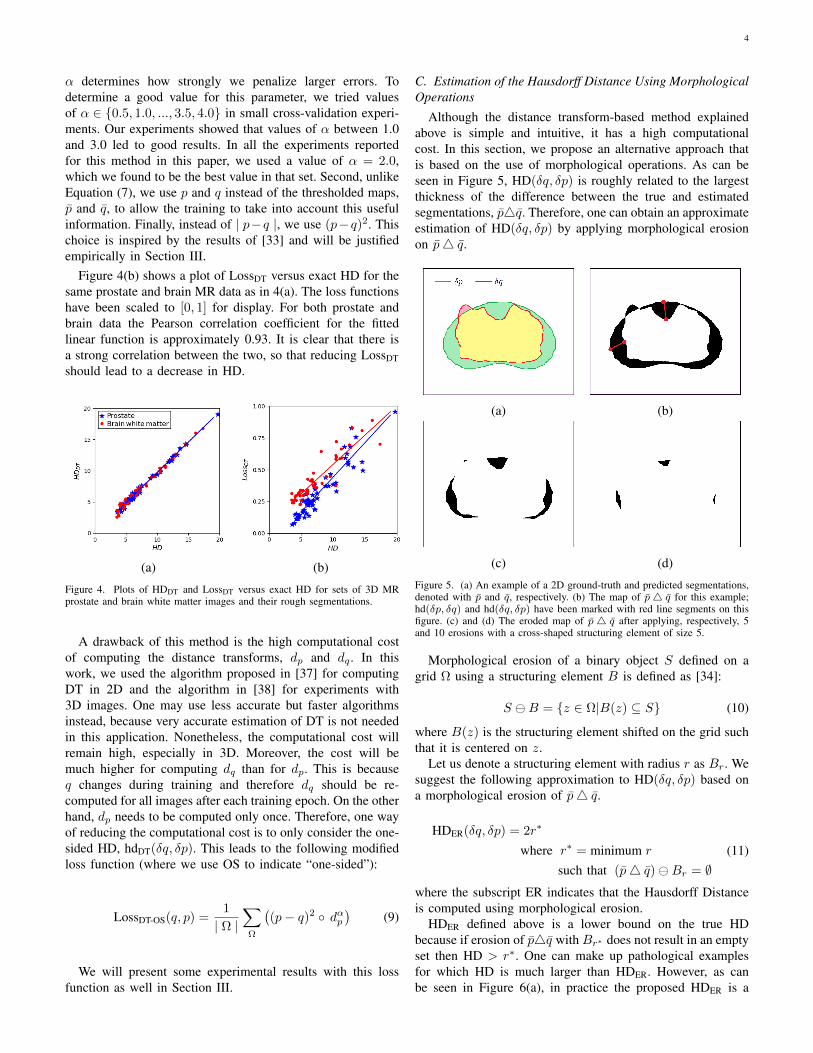
For LossCV, the choice of the set of radius values, R, can beconsidered as a hyper-parameter, which should be chosen foreach application based on the expected range of segmentationerrors. As we have mentioned above, the choice of R willaffect both the segmentation accuracy and computational time.To give the reader a sense of this trade-off, in Table II we haveshown the results of some experiments on 2D prostate ultra-sound and 3D Pancreas CT with different R. Some conclusionscan be drawn from these results. First, as we speculated inSection II-D, no gain is achieved by using kernels of everysize. This can be seen by comparing the results obtainedwith R = 3, 6, 9, . . . , 18 versus R = 3, 4, 5, . . . , 18 for2D prostate ultrasound dataset and by comparing the resultsobtained with R = 3, 6, . . . , 15 versus R = 3, 5, . . . , 15for 3D Pancreas CT dataset. Using more tightly-packed valuesof R will only increase the computational cost without sub-stantially improving the segmentation results. The results inTable II also show that the segmentation performance is notvery sensitive to the choice of R. In particular, for both datasetsused in these experiments, all choices of R resulted in muchsmaller HD than with fDSC(q, p) (as shown in Table I). TableI above also showed that the same choice of R = 3, 6, 9led to very good results on three different datasets of 3Dprostate MRI, 3D liver CT and 3D pancreas CT. This is furtherevidence that this method is not highly sensitive to the choice

9

2D prostate ultrasound

3D prostate MRI

3D Liver CT

3D Pancreas CT

fDSC fDTHD fER

HD fCVHD

Figure 9. Selected images from each dataset and the boundaries of the segmentations produced by different loss functions (in blue) and the ground-truthsegmentation (in red). For the 3D images, we have shown the slice on which fDSC had the largest segmentation error.

of R.

Our proposed DT-based loss function, fDTHD , is based on a

weighting of the segmentation errors, where larger distanceerrors are weighted more strongly. This approach seems to be

the opposite of what some previous studies have proposed.For example, for cell segmentation in [29] and for prostatesegmentation in [30], it has been suggested that larger weightsbe assigned to the pixels that are closer to the boundary of the

10

Table IITHE RESULTS OF EXPERIMENTS WITH VARIOUS CHOICES OF THE PARAMETER R IN LOSSCV ON TWO DIFFERENT DATASETS. FOR EACH DATASET, THE

FIRST ROW SHOWS THE RESULT WITH OUR DEFAULT CHOICE OF R WHICH WAS PRESENTED IN TABLE I. THE LAST ROW FOR EACH DATASET SHOWS THERESULT OBTAINED WITH fDSC (ALSO FROM TABLE I) FOR EASY COMPARISON.

Dataset R DSC HD (mm) Training time (h)

2D prostate ultrasound

R = 3, 6, 9, . . . , 18 0.941± 0.036 2.7± 1.8 4.1R = 3, 6, 9, . . . , 30 0.943± 0.030 2.7± 1.6 9.8R = 3, 6, 9 0.936± 0.045 3.0± 2.2 3.8R = 3, 4, 5, . . . , 18 0.940± 0.035 2.7± 1.8 12.0R = 3, 4, 5, . . . , 30 0.944± 0.032 2.6± 1.6 20.4fDSC(q, p) 0.932± 0.039 4.3± 2.8 3.2

3D Pancreas CT

R = 3, 6, 9 0.780± 0.055 21.7± 11.0 34R = 3, 6, . . . , 15 0.790± 0.056 21.2± 10.7 51R = 3, 6 0.772± 0.082 24.0± 12.8 28R = 3, 5, . . . , 9 0.779± 0.050 21.4± 10.6 40R = 3, 5, . . . , 15 0.788± 0.061 21.3± 10.1 63fDSC(q, p) 0.752± 0.120 32.1± 17.0 22

Figure 10. A plot of the mean HD on the test data for the 2D TRUS images ofprostate as a function of the training epoch number for different loss functions.

ground-truth segmentation. To test this alternate approach, weused the following loss function, which is similar to the lossfunction suggested in [29]:

Loss†DT(q, p) =1

| Ω |∑Ω

((p− q)2 exp

(−d2p

2σ2

))(18)

Our observations show that although this loss function mayslightly improve the DSC on some datasets, in general it hasno significant positive effect on HD, which is the focus ofthis work. For example, with the above loss function (with anadded DSC loss term as in Equation (17)), on the 2D TRUSprostate data we achieved DSC and HD of 0.938 ± 0.035and 4.0 ± 2.7 mm, respectively. Paired t-tests showed thatHD was significantly larger than our three HD-based lossfunctions and DSC was not significantly different from thoseobtained with other loss functions on this dataset. Therefore,compared with our proposed loss functions, assigning largerweights to the pixels closer to the ground-truth boundaryharms the segmentation performance in terms of HD. It isworth pointing out that the main challenge in [29] was tosegment the boundaries of the object of interest (cells), which

could justify a loss function as in Equation (18). Moreover,unlike [29], [30], our loss functions include a DSC loss term,which means that the comparison of our results with thosestudies is not quite fair.

Another distinct aspect of our proposed HD-based lossfunctions is that they are based on the squared difference of theprobability maps, i.e., (p − q)2, whereas medical image seg-mentation methods typically work with the cross-entropy. Ourchoice of the `2-norm was motivated by the results reported insome recent studies [33], [47], [48]. These studies have shownthat loss functions based on hinge loss, squared hinge loss, and`1 and `2 norms may lead to superior results in different deeplearning models. Inspired by these studies, and because noneof them had considered the application of image segmentation,we conducted a set of experiments to examine the usefulnessof these formulations in our application. Figure 11 shows anexample of our observations. In this experiment, we replacedthe squared difference term (p − q)2 in the DT-based lossfunction (Equation (8)) with some of the alternatives proposedin [33], [47], [48]. As can be seen in this figure, `2 loss,hinge loss, and squared hinge loss all perform better than thecross-entropy loss, which is widely used in CNN-based imagesegmentation methods. It was based on such observations thatwe built our HD-based loss functions (Equations (8), (12),and (14)) upon the squared difference, (p− q)2. Overall, ourobservation are in line with those reported in [33]. However,we observed that the `2 loss gives slightly better results thanthe hinge and squared hinge losses and that the `1 loss is notvery poor either, whereas the authors of [33] found that the `1loss was very poor and the hinge losses were slightly betterthan the `2 loss. We think that the most likely reason for thesedifferences is the extra DSC loss term in our work. Moreover,our image segmentation problem is quite different from theapplications considered in [33].

Overall, the results reported in Table I are close to or betterthan the results reported by many recent studies. On the 2DTRUS prostate image data, our results in terms of HD aremuch better than those reported in [49], [50] on the samedataset, where the authors have reported HD of above 5 mm

11

Figure 11. Plots of Dice Similarity Coefficient and Hausdorff Distance onthe 2D TRUS images of the prostate for different formulations of the distancetransform-based loss function.

using two different methods. For prostate segmentation in 3DMRI, most studies have only reported DSC. Some studies havereported the 95th-percentile of HD within an image [31], [51],[52]. Note that this is different from the inter-patient 90th-percentile of HD that we have reported in this paper. Themean of the 95th-percentile intra-patient HD reported in arecent comparison of several state of the art methods is inthe range 4.9− 7.6 mm [52], whereas this quantity computedon the test data with the model trained using fDT

HD(q, p) inour work is 4.70 ± 0.97 mm. Incidentally, the lowest HD inthe comparison published in [52] was achieved by a methodfrom our own group that has not been published yet. For liversegmentation in CT, the reported values of HD vary greatlybetween 24 mm and 119 mm [53]. Our best result, as can beseen in Table I is 25.1 mm. For pancreas segmentation, moststudies only report DSC and the mean or root-mean-squareof surface distance. A recent study reported values of HD inthe range 17.7−22.2 mm [54], compared with our best resultof 21.3 mm. Pancreas segmentation is considered to be verychallenging and most studies have reported a DSC of below0.80. Recently some works have achieved DSC values of wellabove 0.80 [55], [56]. We should note, however, that thosestudies have used more elaborate machinery such as a separatemodel to identify the location of the pancreas or iterativerefinement strategies. For example, the work that has reportedmean HDs as low as 17.7 mm is a multi-stage method that uses

multiple CNN models and other machine learning methods tolocalize the pancreas, identify boundary cues, and aggregatesegmentation cues [54]. We should stress that the goal of thepresent study was not to achieve the state of the art results insegmentation of different organs and imaging modalities; onecould always achieve better results by fine-tuning the networkstructure or employing a more sophisticated methodology thatis tailored to the specific organ and imaging modality. Ourexperiments were intended to show that the proposed lossfunctions could lead to a significant reduction in HD. Thatis why we have adopted standard segmentation models andtraining procedures in order to eliminate, as much as possible,other confounding factors and study the effectiveness of theproposed loss functions.

We further compared our proposed loss functions on the testdata of the PROMISE12 challenge [43]. In this experiment, wetrained our CNN model with different loss functions on the 50training images provided by this challenge and tested on the30 test images for which the true segmentation is only knownto the challenge organizers. A summary of the results of thisexperiment is presented in Table III. The trends observed inthis Table are similar to those in Table I. The DSC scoresachieved on this dataset are better than those in Table I andthey are very similar for all four loss functions. Comparedwith fDSC, all three proposed HD-based loss functions havesubstantially reduced the mean, standard deviation, and themaximum of HD95. The reduction in HD for 3D prostateMRI data in Table I was in the range 18 − 23%, whereasthe reduction in HD95 in III was in the range 10− 15%. Thisis, at least in part, because HD95 ignores the top 5% withthe largest surface distance error. Therefore HD95 does notreflect the very largest segmentation errors that HD represent.We cannot compute the HD for this dataset because we donot have the ground-truth. Nonetheless, these results showthat our proposed method is capable of reducing not only thevery largest segmentation error but also to consistently reducelarge segmentation errors as quantified by HD95. Comparedwith other recently-published papers on the same dataset, ourachieved HD95 values are significantly better. Two recently-published methods evaluated on the same dataset have beenincluded in Table III. As we pointed out above, a recent studycompared 10 state of the art methods on this dataset andreported the HD95 values in the range 4.9 − 7.6 mm [52],whereas our HD-based loss functions resulted in HD valuesas low as 4.26.

We also applied our methods on the MRI brain segmentationdata from the iSeg-2017 challenge [58]. The goal of this chal-lenge is to segment infant brain MR images into four classes:1) white matter (WM), 2) gray matter (GM), 3) cerebrospinalfluid (CSF), and 4) background. The challenge organizersallow a maximum of two submissions per team. Because basedon Table I fDT

HD and fERHD were, overall, the best and worst of

our three HD-based loss functions, we evaluated these twoloss functions on this challenge. Our results have been shownin Table IV. As a comparison with another method, we haveincluded the results obtained by the recently published methodin [59], which at the time of our participation in this challenge(March 2019) has achieved the highest Dice score on all three

12

Table IIIA SUMMARY OF THE COMPARISON OF THE PROPOSED LOSS FUNCTIONS ON THE TEST DATA FROM THE PROMISE12 CHALLENGE [43]. N.R. STANDS

FOR “NOT REPORTED”.

Loss Function DSC HD95 (mm) Max. of HD95 (mm)fDSC(q, p) 0.908 ± 0.032 5.00± 2.16 11.3fDT

HD(q, p) 0.902± 0.026 4.28± 1.05 7.8fER

HD(q, p) 0.904± 0.023 4.48± 1.46 8.8fCV

HD (q, p) 0.902± 0.025 4.26 ± 1.03 7.6

Yu et al., 2017, [57] 0.894 5.54 N.R.Brosch et al., 2018, [52] 0.905 4.94 N.R.

structures among all participating teams. To also compare ourother two loss functions (fDSC and fCV

HD ) we performed a five-fold cross-validation on the training images of this challenge.The results of this experiment have also been included in TableIV.

As can be seen from this table, fDTHD and fER

HD achieve a lowerHD than the method of [59] on all three structures, with oneexception of loss function fER

HD(q, p) on CSF segmentation).Our best performing loss function (fDT

HD(q, p)) has reduced HDcompared with [59] by approximately 1.5%, 35%, and 4.2%,respectively on CSF, GM, and WM, respectively. Overall,compared with all participating teams in this challenge, ourbest achieved HD was ranked 1st in CSF segmentation, 3rd inGM segmentation, and 6th in WM segmentation. We shouldnote that we used the basic 3D U-Net that we had used forsegmentation of the other datasets in this study, without anymodifications. On the other hand, other participating teamshave developed methods specifically for this challenge. Forexample, the leading method in [59] has used a CNN-basedpatch-level training and prediction aggregation method spe-cially designed for this brain MRI segmentation task. A betterway of assessing the effect of our proposed HD-based lossfunctions is to compare with the results obtained with fDSC inour five-fold cross-validation experiments reported in the sameTable. Compared with fDSC, our best performing loss function,fDT

HD , reduces HD by 15%, 35%, and 23%, respectively onCSF, GM, and WM, respectively, which represent substantialimprovements. The other two HD-based loss functions, fER

HDand fCV

HD , also reduce the HD (compared with fDSC) by 8%to 33% while achieving DSC values that are very close to orbetter than fDSC.

As we have argued throughout the paper, minimizing HDdirectly can be tricky and counter-productive. This is why wehave proposed relaxed loss functions that are based on HD,instead of minimizing HD directly. Moreover, we augmentedour HD-based loss functions with DSC loss, which is basedon the amount of overlap between the ground-truth and esti-mated segmentation maps. Nonetheless, one would be curiousto know how the proposed HD-based loss functions wouldperform without the added DSC loss term. We performedexperiments to empirically understand the training of CNNsegmentation methods with these loss functions. We observedthat it was possible to train CNN segmentation methods withthese loss functions. However, this required a more carefultuning of the learning rate and using a much smaller learningrate in the first few training epochs. Moreover, we observed

that the segmentation results were always better when the DSCloss term was included.

Here we briefly summarize the results obtained on twoof our datasets. For the 2D prostate ultrasound data, theHD values achieved using fDT

HD , fERHD, and fCV

HD without theDSC loss term were, respectively, 2.9 ± 1.8, 3.3 ± 2.4, and2.9±2.2 and the DSC values were, respectively, 0.930±0.038,0.921 ± 0.048, and 0.923 ± 0.040. These results are slightlyworse than those reported in Table I for these methods withthe added DSC loss term. Nonetheless, it is interesting tonote that these HD values are still much better than 4.3± 2.8achieved with fDSC as shown in Table I. For the 3D pancreasCT data, the HD values achieved using fDT

HD , fERHD, and fCV

HDwithout the DSC loss term were, respectively, 22.9 ± 13.8,27.6 ± 13.4, and 22.7 ± 12.0 and the DSC values were,respectively, 0.779±0.058, 0.750±0.068, and 0.772±0.054.These results also show that better results can be obtained byincluding the DSC loss term. Nonetheless, these HD valuesare still much smaller than 32.1± 17.0 obtained with fDSC asshown in Table I.

Using the HD-based loss functions alone is equivalent tosetting λ = 0 in Eq. 17. Using the DSC loss alone, i.e., fDSCcorresponds to a very large λ. As we mentioned above, in ourexperiments we update the value of λ such that the two lossterms (i.e., the HD-based loss term and the DSC loss term)have equal weight. In Figure 12 we have shown the effectof changing this weighting on the example of training withfDT

HD on the 2D prostate ultrasound data. This figure showsthat for this specific case this choice is close to optimal andthat choosing λ such that the ratio of the DSC loss term tothe HD-based loss term is in the range [0.1, 2] leads to goodsegmentation results in terms of both HD and DSC. Figure 13shows the change in the value of λ over training epochs forthe three HD-based loss functions on the 3D liver CT data.We observed similar trends on the other datasets. The valuesof λ have been normalized such that the value at the end oftraining is approximately equal to one, so that the curves canbe shown on the same plot. The overall trend is that the valueof λ in the early training epochs is larger. This is because atthe start of training there are many false positives far from thesegmentation boundaries, which increases the HD-based lossterm.

We further tried training with the “exact HD” as the lossfunction, instead of our proposed relaxed HD-based lossfunctions. In these experiments, we tried training models usingEquation (7) as the loss function for 2D and 3D datasets.

13

Table IVA SUMMARY OF THE COMPARISON OF THE PROPOSED LOSS FUNCTIONS ON THE TEST DATA FROM THE ISEG-2017 CHALLENGE.

CSF GM WM

Experiment Loss Function DSC HD DSC HD DSC HD

Evaluated on the test data of iSeg2017fDT

HD(q, p) 0.945 8.720 0.911 6.212 0.890 6.812

fERHD(q, p) 0.947 9.434 0.915 6.832 0.894 6.988

Hashemi et al., 2019 [59] 0.960 8.850 0.926 9.557 0.907 7.104

Evaluated on the training data ofiSeg2017 via five-fold cross-validation

fDSC(q, p) 0.950 10.224 0.914 9.320 0.905 8.802fDT

HD(q, p) 0.942 8.725 0.910 6.101 0.894 6.816

fERHD(q, p) 0.949 9.408 0.910 6.845 0.899 6.983fCV

HD (q, p) 0.951 8.733 0.922 6.225 0.908 6.854

Figure 12. The change in the segmentation performance on the 2D prostateultrasound data using loss function fDT

HD with different values of λ. Thehorizontal axis is a function of λ/λ∗, where λ∗ is our default setting whichis chosen such that the HD-based and DSC loss terms have equal weights.

Figure 13. Change in the value of λ with training epochs for the 3D liverCT dataset. The values of λ for the three loss functions have been normalizedsuch that the value at the end of training is approximately equal to one.

However, the models never converged to a meaningful stateregardless of the learning rate. This is very much expectedbecause HD aims at minimizing the error at one single pointwith the largest error. We have presented arguments againstusing HD as a loss function in Section I and reviewed someof the computer vision literature in this regard. Moreover,

with randomly-initialized deep learning models, minimizingonly the largest error cannot be justified and our observationsconfirm this.

We have successfully tested our method on five differentdatasets which include organs of different sizes and shapes indifferent imaging modalities. Nonetheless, we cannot claimthat our method will be successful in all medical imagesegmentation tasks. Indeed, the range of anatomical shapes andthe level of detail in medical image segmentation is very wide.Hence, application of our loss functions to other organs mayneed modifications. For example, in some applications suchas vessel segmentation, recent studies have used additionalmodules such as probabilistic graphical models on top ofCNNs to achieve good results [60], [61]. In such applications,our proposed methods might need application-specific modifi-cations. A comprehensive experimental study or review of therange of applications for our proposed method and a discussionof all application-specific issues is beyond the scope of thispaper.

IV. CONCLUSION

Our results show that all three proposed HD-based lossfunctions can lead to statistically significant reductions in HDin the segmentation of 2D and 3D medical images of differentimaging modalities. Therefore, the proposed methods can bevery useful in applications such as multimodal image registra-tion where large segmentation errors can be very harmful. Tothe best of our knowledge, none of the three methods proposedin this work for estimating HD and the three loss functionsproposed for training segmentation algorithms have appearedin previous publications. The distance transform-based loss,fDT

HD , is the most intuitive of the three formulations and leadsto very good results, but it also substantially increases thecomputational load. The loss based on morphological erosion,fER

HD, is computationally less expensive, but not as effectiveas the other two losses. The loss based on convolutions withkernels of increasing sizes, fCV

HD , leads to very good resultsand it can be computationally much less demanding thanthe distance transform-based loss if one properly limits themaximum size and the number of convolutional kernels thatare used. Overall, the decision on which of the three lossfunctions to use depends on the application. For example, for2D images the cost of computing the distance transforms is notsubstantial and one may use fDT

HD . For 3D images, fERHD and fCV

HD

14

may be better options, with fCVHD offering better segmentation

performance at the cost of longer training times.To the best of our knowledge, this is the first work to aim

at reducing HD in medical image segmentation. The methodspresented in this paper may be improved in several ways.Faster implementation of the HD-based loss functions andmore accurate implementation of the loss function based onmorphological erosion would be useful. Moreover, extensionof the methods for other applications such as vessel segmen-tation could also be pursued.

ACKNOWLEDGMENT

This project is funded by the Natural Science and Engi-neering Research Council of Canada (NSERC), the CanadianInstitutes of Health Research (CIHR), and the Prostate CancerCanada (PCC). We would like to thank the support fromthe Charles Laszlo Chair in Biomedical Engineering held byProfessor S. Salcudean.

REFERENCES

[1] K. D. Toennies, Guide to Medical Image Analysis. Springer, 2017.[2] S. K. Zhou, Medical Image Recognition, Segmentation and Parsing:

Machine Learning and Multiple Object Approaches. Academic Press,2015.

[3] H. R. Roth, C. Shen, H. Oda, M. Oda, Y. Hayashi, K. Misawa,and K. Mori, “Deep learning and its application to medical imagesegmentation,” Medical Imaging Technology, vol. 36, no. 2, pp. 63–71,2018.

[4] G. Wang, W. Li, M. A. Zuluaga, R. Pratt, P. A. Patel, M. Aertsen,T. Doel, A. L. David, J. Deprest, S. Ourselin, and T. Vercauteren, “In-teractive medical image segmentation using deep learning with image-specific fine tuning,” IEEE Transactions on Medical Imaging, vol. 37,no. 7, pp. 1562–1573, July 2018.

[5] W. R. Crum, O. Camara, and D. L. Hill, “Generalized overlap measuresfor evaluation and validation in medical image analysis,” IEEE Trans-actions on Medical Imaging, vol. 25, no. 11, pp. 1451–1461, 2006.

[6] A. A. Taha and A. Hanbury, “Metrics for evaluating 3d medical imagesegmentation: analysis, selection, and tool,” BMC Medical Imaging,vol. 15, no. 1, p. 29, 2015.

[7] R. T. Rockafellar and R. J.-B. Wets, Variational Analysis. SpringerScience & Business Media, 2009, vol. 317.

[8] E. Smistad, T. L. Falch, M. Bozorgi, A. C. Elster, and F. Lindseth,“Medical image segmentation on GPUs–a comprehensive review,” Med-ical image analysis, vol. 20, no. 1, pp. 1–18, 2015.

[9] T. Heimann and H.-P. Meinzer, “Statistical shape models for 3d medicalimage segmentation: A review,” Medical Image Analysis, vol. 13, no. 4,pp. 543 – 563, 2009.

[10] V. Caselles, R. Kimmel, and G. Sapiro, “Geodesic active contours,”International Journal of Computer Vision, vol. 22, no. 1, pp. 61–79,1997.

[11] M. Kass, A. Witkin, and D. Terzopoulos, “Snakes: Active contourmodels,” International Journal of Computer Vision, vol. 1, no. 4, pp.321–331, 1988.

[12] J. L. Marroquin, B. C. Vemuri, S. Botello, E. Calderon, andA. Fernandez-Bouzas, “An accurate and efficient bayesian method forautomatic segmentation of brain MRI,” IEEE Transactions on MedicalImaging, vol. 21, no. 8, pp. 934–945, 2002.

[13] H. Park, P. H. Bland, and C. R. Meyer, “Construction of an abdominalprobabilistic atlas and its application in segmentation,” IEEE Transac-tions on Medical Imaging, vol. 22, no. 4, pp. 483–492, 2003.

[14] N. Makni, N. Betrouni, and O. Colot, “Introducing spatial neighbour-hood in evidential c-means for segmentation of multi-source images: Ap-plication to prostate multi-parametric mri,” Information Fusion, vol. 19,pp. 61–72, 2014.

[15] S. Pereira, A. Pinto, J. Oliveira, A. M. Mendrik, J. H. Correia, andC. A. Silva, “Automatic brain tissue segmentation in mr images usingrandom forests and conditional random fields,” Journal of NeuroscienceMethods, vol. 270, pp. 111–123, 2016.

[16] F. R. Schmidt and Y. Boykov, “Hausdorff distance constraint for multi-surface segmentation,” in European Conference on Computer Vision.Springer, 2012, pp. 598–611.

[17] M.-P. Dubuisson and A. K. Jain, “A modified hausdorff distance forobject matching,” in Proceedings of 12th International Conference onPattern Recognition. IEEE, pp. 566–568.

[18] C.-H. T. Yang, S.-H. Lai, and L.-W. Chang, “Hybrid image matchingcombining hausdorff distance with normalized gradient matching,” Pat-tern Recognition, vol. 40, no. 4, pp. 1173–1181, 2007.

[19] D. P. Huttenlocher, G. A. Klanderman, and W. J. Rucklidge, “Comparingimages using the hausdorff distance,” IEEE Transactions on PatternAnalysis and Machine Intelligence, vol. 15, no. 9, pp. 850–863, 1993.

[20] K. J. Kirchberg, O. Jesorsky, and R. W. Frischholz, “Genetic model opti-mization for hausdorff distance-based face localization,” in InternationalWorkshop on Biometric Authentication. Springer, 2002, pp. 103–111.

[21] D.-G. Sim, O.-K. Kwon, and R.-H. Park, “Object matching algorithmsusing robust hausdorff distance measures,” IEEE Transactions on ImageProcessing, vol. 8, no. 3, pp. 425–429, 1999.

[22] H. Tan and Y.-J. Zhang, “A novel weighted hausdorff distance for facelocalization,” Image and Vision Computing, vol. 24, no. 7, pp. 656–662,2006.

[23] C. Knauer, K. Kriegel, and F. Stehn, “Minimizing the weighted directedhausdorff distance between colored point sets under translations andrigid motions,” Theoretical Computer Science, vol. 412, no. 4-5, pp.375–382, 2011.

[24] D. Dimitrov, C. Knauer, K. Kriegel, and F. Stehn, “Approximation algo-rithms for a point-to-surface registration problem in medical navigation,”in International Workshop on Frontiers in Algorithmics. Springer, 2007,pp. 26–37.

[25] G. Litjens, T. Kooi, B. E. Bejnordi, A. A. A. Setio, F. Ciompi,M. Ghafoorian, J. A. van der Laak, B. van Ginneken, and C. I. Sanchez,“A survey on deep learning in medical image analysis,” Medical ImageAnalysis, vol. 42, no. Supplement C, pp. 60 – 88, 2017.

[26] F. Milletari, A. Rothberg, J. Jia, and M. Sofka, Integrating StatisticalPrior Knowledge into Convolutional Neural Networks. Cham: SpringerInternational Publishing, 2017, pp. 161–168.

[27] D. Karimi, G. Samei, C. Kesch, G. Nir, and S. E. Salcudean, “Prostatesegmentation in MRI using a convolutional neural network architectureand training strategy based on statistical shape models,” InternationalJournal of Computer Assisted Radiology and Surgery, vol. 13, no. 8,pp. 1211–1219, Aug 2018.

[28] J. Long, E. Shelhamer, and T. Darrell, “Fully convolutional networksfor semantic segmentation,” in Proceedings of the IEEE Conference onComputer Vision and Pattern Recognition, 2015, pp. 3431–3440.

[29] O. Ronneberger, P. Fischer, and T. Brox, “U-net: Convolutional networksfor biomedical image segmentation,” in International Conference onMedical Image Computing and Computer-Assisted Intervention, 2015,pp. 234–241.

[30] E. M. A. Anas, S. Nouranian, S. S. Mahdavi, I. Spadinger, W. J.Morris, S. E. Salcudean, P. Mousavi, and P. Abolmaesumi, “Clinicaltarget-volume delineation in prostate brachytherapy using residual neuralnetworks,” in International Conference on Medical Image Computingand Computer-Assisted Intervention. Springer, 2017, pp. 365–373.

[31] F. Milletari, N. Navab, and S.-A. Ahmadi, “V-net: Fully convolutionalneural networks for volumetric medical image segmentation,” in 3DVision (3DV), 2016 Fourth International Conference on. IEEE, 2016,pp. 565–571.

[32] S. S. M. Salehi, D. Erdogmus, and A. Gholipour, “Tversky loss functionfor image segmentation using 3d fully convolutional deep networks,”in International Workshop on Machine Learning in Medical Imaging.Springer, 2017, pp. 379–387.

[33] K. Janocha and W. M. Czarnecki, “On loss functions for deep neuralnetworks in classification,” arXiv preprint arXiv:1702.05659, 2017.

[34] R. Szeliski, Computer Vision: Algorithms and Applications. SpringerScience & Business Media, 2010.

[35] T. Jech, “Set theory: The third millennium edition, revised and expanded,3rd,” Springer Monographs in Mathematics, Springer-Verlag BerlinHeidelberg New York, 2002.

[36] A. A. Taha and A. Hanbury, “An efficient algorithm for calculating theexact hausdorff distance,” IEEE Transactions on Pattern Analysis andMachine Intelligence, vol. 37, no. 11, pp. 2153–2163, 2015.

[37] P. Felzenszwalb and D. Huttenlocher, “Distance transforms of sampledfunctions,” Cornell University, Tech. Rep., 2004.

[38] C. R. Maurer, R. Qi, and V. Raghavan, “A linear time algorithmfor computing exact euclidean distance transforms of binary imagesin arbitrary dimensions,” IEEE Transactions on Pattern Analysis andMachine Intelligence, vol. 25, no. 2, pp. 265–270, 2003.

15

[39] J. Mazille, “Mathematical morphology and convolutions,” Journal ofMicroscopy, vol. 156, no. 1, pp. 3–13, 1989.

[40] M. Razaz and D. Hagyard, “Efficient convolution based algorithms forerosion and dilation.” in NSIP, 1999, pp. 360–363.

[41] S. Foucart and H. Rauhut, A Mathematical Introduction to CompressiveSensing. Birkhauser, 2013.

[42] S. S. Mahdavi, N. Chng, I. Spadinger, W. J. Morris, and S. E. Salcud-ean, “Semi-automatic segmentation for prostate interventions,” MedicalImage Analysis, vol. 15, no. 2, pp. 226–237, 2011.

[43] G. Litjens, R. Toth, W. van de Ven, C. Hoeks, S. Kerkstra, B. vanGinneken, G. Vincent, G. Guillard, N. Birbeck, J. Zhang, R. Strand,F. Malmberg, Y. Ou, C. Davatzikos, M. Kirschner, F. Jung, J. Yuan,W. Qiu, Q. Gao, P. Edwards, B. Maan, F. van der Heijden, S. Ghose,J. Mitra, J. Dowling, D. Barratt, H. Huisman, and A. Madabhushi,“Evaluation of prostate segmentation algorithms for mri: The promise12challenge,” Medical Image Analysis, vol. 18, no. 2, pp. 359 – 373, 2014.

[44] N. J. Tustison, B. B. Avants, P. A. Cook, Y. Zheng, A. Egan, P. A.Yushkevich, and J. C. Gee, “N4itk: Improved n3 bias correction,” IEEETransactions on Medical Imaging, vol. 29, no. 6, pp. 1310–1320, June2010.

[45] O. Cicek, A. Abdulkadir, S. S. Lienkamp, T. Brox, and O. Ronneberger,“3d u-net: learning dense volumetric segmentation from sparse anno-tation,” in International Conference on Medical Image Computing andComputer-Assisted Intervention. Springer, 2016, pp. 424–432.

[46] D. P. Kingma and J. Ba, “Adam: A method for stochastic optimiza-tion,” in Proceedings of the 3rd International Conference on LearningRepresentations (ICLR), 2014.

[47] C.-Y. Lee, S. Xie, P. Gallagher, Z. Zhang, and Z. Tu, “Deeply-supervisednets,” in Artificial Intelligence and Statistics, 2015, pp. 562–570.

[48] Y. Tang, “Deep learning using linear support vector machines,” arXivpreprint arXiv:1306.0239, 2013.

[49] S. Nouranian, S. S. Mahdavi, I. Spadinger, W. J. Morris, S. E. Salcudean,and P. Abolmaesumi, “A multi-atlas-based segmentation framework forprostate brachytherapy,” IEEE Transactions on Medical Imaging, vol. 34,no. 4, pp. 950–961, 2015.

[50] S. Nouranian, M. Ramezani, I. Spadinger, W. J. Morris, S. E. Salcudean,and P. Abolmaesumi, “Learning-based multi-label segmentation of tran-srectal ultrasound images for prostate brachytherapy,” IEEE Transactionson Medical Imaging, vol. 35, no. 3, pp. 921–932, 2016.

[51] A. Salimi, M. A. Pourmina, and M.-S. Moin, “Fully automatic prostatesegmentation in mr images using a new hybrid active contour-basedapproach,” Signal, Image and Video Processing, pp. 1–9, 2018.

[52] T. Brosch, J. Peters, A. Groth, T. Stehle, and J. Weese, “Deep learning-based boundary detection for model-based segmentation with applica-tion to mr prostate segmentation,” in Medical Image Computing andComputer Assisted Intervention – MICCAI 2018, A. F. Frangi, J. A.Schnabel, C. Davatzikos, C. Alberola-Lopez, and G. Fichtinger, Eds.Cham: Springer International Publishing, 2018, pp. 515–522.

[53] P. F. Christ, M. E. A. Elshaer, F. Ettlinger, S. Tatavarty, M. Bickel,P. Bilic, M. Rempfler, M. Armbruster, F. Hofmann, M. D’Anastasi et al.,“Automatic liver and lesion segmentation in ct using cascaded fullyconvolutional neural networks and 3d conditional random fields,” inInternational Conference on Medical Image Computing and Computer-Assisted Intervention. Springer, 2016, pp. 415–423.

[54] H. R. Roth, L. Lu, N. Lay, A. P. Harrison, A. Farag, A. Sohn, and R. M.Summers, “Spatial aggregation of holistically-nested convolutional neu-ral networks for automated pancreas localization and segmentation,”Medical Image Analysis, vol. 45, pp. 94–107, 2018.

[55] H. Roth, M. Oda, N. Shimizu, H. Oda, Y. Hayashi, T. Kitasaka,M. Fujiwara, K. Misawa, and K. Mori, “Towards dense volumetricpancreas segmentation in ct using 3d fully convolutional networks,” inMedical Imaging 2018: Image Processing, vol. 10574. InternationalSociety for Optics and Photonics, 2018, p. 105740B.

[56] Y. Zhou, L. Xie, W. Shen, Y. Wang, E. K. Fishman, and A. L. Yuille, “Afixed-point model for pancreas segmentation in abdominal ct scans,” inInternational Conference on Medical Image Computing and Computer-Assisted Intervention. Springer, 2017, pp. 693–701.

[57] L. Yu, X. Yang, H. Chen, J. Qin, and P. A. Heng, “Volumetric convnetswith mixed residual connections for automated prostate segmentationfrom 3d MR images,” in Thirty-first AAAI conference on artificialintelligence, 2017.

[58] L. Wang, D. Nie, G. Li, E. Puybareau, J. Dolz, Q. Zhang, F. Wang,J. Xia, Z. Wu, J. Chen et al., “Benchmark on automatic 6-month-oldinfant brain segmentation algorithms: The iseg-2017 challenge,” IEEETransactions on Medical Imaging, 2019.

[59] S. R. Hashemi, S. S. M. Salehi, D. Erdogmus, S. P. Prabhu, S. K.Warfield, and A. Gholipour, “Asymmetric loss functions and deep

densely-connected networks for highly-imbalanced medical image seg-mentation: Application to multiple sclerosis lesion detection,” IEEEAccess, vol. 7, pp. 1721–1735, 2019.

[60] H. Fu, Y. Xu, D. W. K. Wong, and J. Liu, “Retinal vessel segmentationvia deep learning network and fully-connected conditional randomfields,” in Biomedical Imaging (ISBI), 2016 IEEE 13th InternationalSymposium on. IEEE, 2016, pp. 698–701.

[61] S. Y. Shin, S. Lee, I. D. Yun, and K. M. Lee, “Deep vessel segmentationby learning graphical connectivity,” arXiv preprint arXiv:1806.02279,2018.