Embed Size (px)
Citation preview
URBAN INSTITUTE
http://www.urban.org/
January 2015
2100 M Street NW
Washington, DC 20037-1264
Reducing Child Poverty in the US: Costs and Impacts of Policies Proposed by the
Children’s Defense Fund
Linda Giannarelli, Kye Lippold, Sarah Minton, and Laura Wheaton

ABOUT THE URBAN INSTITUTE The nonprofit Urban Institute is dedicated to elevating the debate on social and economic policy. For nearly five decades, Urban scholars have conducted research and offered evidence-based solutions that improve lives and strengthen communities across a rapidly urbanizing world. Their objective research helps expand opportunities for all, reduce hardship among the most vulnerable, and strengthen the effectiveness of the public sector. The Urban Institute is a nonprofit policy research organization. It has been incorporated and is operated as a public charity. It has received official IRS recognition of its tax-exempt status under sections 501(c)(3) and 509(a)(2) of the Internal Revenue Code. The Institute’s federal ID number is 52-0880375. Donations will be tax deductible and may be disclosed to the IRS and the public, unless given anonymously. We are committed to transparent accounting of the resources we receive. In addition to required tax filings, a copy of the Urban Institute’s audited financial statement is available to anyone who requests it.
ACKNOWLEDGEMENTS This project was funded by the Children’s Defense Fund. Caroline Fichtenberg and MaryLee Allen provided full information on the policies to be modeled. However, the technical implementation of the policies was determined by Urban Institute staff. The views expressed are those of the authors and should not be attributed to the Urban Institute, its trustees, or its funders. Information presented here is derived in part from the Transfer Income Model, Version 3 (TRIM3) and associated databases. TRIM3 requires users to input assumptions and/or interpretations about economic behavior and the rules governing federal programs. Therefore, the conclusions presented here are attributable only to the authors of this report. The authors owe special thanks to Sheila Zedlewski for her thoughtful contributions in the initial stages of the project, and to Joyce Morton and Silke Taylor, for the skilled computer programming that was essential to the analysis. Other Urban Institute colleagues—Elaine Maag, Christin Durham, Erika Huber, Elissa Cohen, Martha Johnson, Paul Johnson, Kara Harkins, Jessica Kelly, Michael Martinez-Schiferl, Caleb Quakenbush, and Anne Whitesell—participated in developing the baseline simulations that underlie this analysis. Lorraine Blatt assisted with table preparation. We are very grateful to the US Department of Health and Human Services, Office of the Assistant Secretary for Planning and Evaluation (HHS/ASPE), for the ongoing support they provide to maintain the CPS-based TRIM3 model, and for the fact that they allow the HHS-funded TRIM3 baseline simulations to be used as the foundation for other analyses such as this one.
Copyright © January 2015
URBAN INSTITUTE
Contents
Executive Summary ...................................................................................................................... 1
Introduction ................................................................................................................................... 8 Data and Simulation Methods ..................................................................................................... 9
The Current Population Survey ................................................................................................. 10 The TRIM3 Model and the Resources of US Families at the Baseline .................................... 11
The TRIM3 Simulations of Benefits and Taxes ................................................................... 11 Changes since 2010............................................................................................................... 13
Simulation of Alternative Policies ............................................................................................ 15
Child Poverty in 2010 ................................................................................................................. 17 The Importance of Using the SPM ............................................................................................ 17 The SPM Resource Measure ..................................................................................................... 18
The SPM Poverty Thresholds ................................................................................................... 20 Results: Child Poverty in 2010 Using the SPM ........................................................................ 23
Policy Changes to Reduce Child Poverty.................................................................................. 26 Increasing Cash Income ............................................................................................................ 26
Higher Minimum Wage ........................................................................................................ 26
Transitional Jobs ................................................................................................................... 32
Child Support Pass-Through ................................................................................................. 38
Increasing In-Kind Income ........................................................................................................ 42 Expanded Housing Assistance .............................................................................................. 42
SNAP Benefit Increase ......................................................................................................... 48 Reducing Taxes ......................................................................................................................... 53
Expanded Earned Income Tax Credit ................................................................................... 53
Fully Refundable Child Tax Credit ....................................................................................... 59 Higher Child and Dependent Care Tax Credit ...................................................................... 61
Reducing Expenses ................................................................................................................... 64
Expanded Child Care Subsidies ............................................................................................ 64 Combining Policies ................................................................................................................... 71
Minimum Wage and EITC.................................................................................................... 71
Minimum Wage, EITC, and Transitional Jobs ..................................................................... 72 All Policies Combined .......................................................................................................... 75
Summary and Caveats ................................................................................................................ 83 References .................................................................................................................................... 87
Appendix A. Validation of TRIM3 Baseline Simulations ....................................................... 92 Appendix B. Effects of Selected Stimulus Provisions on Child Poverty ................................ 96 Appendix C. Detailed Policy Package Simulation Results ...................................................... 99

URBAN INSTITUTE
Executive Summary
A large portion of US children live in poverty—22 percent according to the official measure, and
18 percent according to the Census Bureau’s Supplemental Poverty Measure (SPM). The SPM
shows that child poverty is alleviated by the current safety net, but despite those benefits child
poverty has risen over the last decade.
Within that context, the Children’s Defense Fund (CDF) contracted with the Urban
Institute to assess the costs and impacts of a variety of policy options that could further reduce
child poverty. The policy options defined by CDF include the following:
Minimum wage increased to a level of $10.10 in 2014 dollars for covered workers, and 70
percent of that level for tipped workers.
Transitional jobs program for unemployed and underemployed people in families with
children: CDF assumed a participation rate of 25 percent for unemployed individuals with
the lowest family incomes.
A full pass-through and disregard of child support income by the Temporary Assistance to
Needy Families (TANF) program, and a $100 monthly child support disregard per child in
the Supplemental Nutrition Assistance Program (SNAP, formerly food stamps).
Expanded access to housing vouchers for low-income households with children: New
vouchers would be available to any household with children with income under 150 percent
of the poverty guideline that also satisfied a test of rent burden, with the assumption that 70
percent of those households would be able to use the voucher.
Increased SNAP benefits for families with children: The maximum SNAP benefit for
families with children would be based on the Low-Cost Food Plan levels computed by the
US Department of Agriculture (USDA) rather than the Thrifty Food Plan currently used,
increasing the maximum benefit by 30 percent.
Expanded Earned Income Tax Credit: The parameters of the credit would be adjusted to
increase the benefits; for example, the maximum credit for a single parent with two children
would increase from $5,036 to $6,042.
Fully refundable Child Tax Credit.
Increased Child and Dependent Care Tax Credit (CDCTC).
Expanded access to child care subsidies for low-income families with children under age 13:
Specifically, child care subsidies would be available to any employed family with income
under 150 percent of the poverty guideline wanting that subsidy.
2
All the options have the potential to directly improve families’ economic well-being in
the same year that the policies are implemented (as opposed to policies such as improved
education with the potential to improve children’s well-being in the medium to longer term).
Urban Institute staff analyzed the CDF policies by applying a microsimulation model—
the Transfer Income Model, version 3 (TRIM3)—to a large representative sample of US
households—the Census Bureau’s Current Population Survey, Annual Social and Economic
Supplement (CPS-ASEC). The TRIM3 model is a comprehensive and detailed model that can
capture both the current operations of tax and benefit programs and the potential impacts of
changes to those programs, which has been used for both national and state-level analyses of the
antipoverty impact of taxes and benefits. The CPS-ASEC data include information on over
75,000 households, and the information can be used to make reliable inferences about impacts on
the entire population; it is the same survey database used to generate official poverty estimates.
The analysis used the CPS-ASEC data that captured families’ incomes and employment during
2010. We applied the TRIM3 model to the survey data to estimate the economic circumstances
of families with children before any of the proposed policies, after each policy individually, and
after all policies combined. TRIM3 captured the direct impacts of policies and the interactions
among policies. For example, the fact that an increase in a family’s earnings affects their tax
liability and the amount of safety net benefits they are eligible to receive. We also used the
model to impose external estimates of the extent to which increased tax credits might increase
labor supply, and the extent to which a minimum wage increase might reduce employment.
To assess the results in terms of poverty, we used the SPM poverty measure. Unlike the
official measure of poverty, which considers only a family’s cash income, the SPM looks at
families’ resources more broadly—including the value of in-kind benefits and refundable tax
credits, but subtracting taxes that a family must pay as well as the cost of child care and other
work expenses for families with employed parents. The SPM allowed all the policies to be
considered using the same metric.
Considering all the policies in combination, the impacts on poverty were as follows:
Overall, the number of children in poverty in 2010 according to the SPM is estimated to fall
from 10.9 million to 4.3 million due to the CDF-proposed policies—a drop of 60 percent.
Among the children who are not raised out of poverty by the policy package, the great
majority—4 million—nevertheless see an increase in family economic resources.
The poverty gap for families with children—the aggregate amount of money by which the
incomes of poor families with children fall below their poverty thresholds—fell from $40.5
billion to $15.0 billion, a drop of 63 percent.
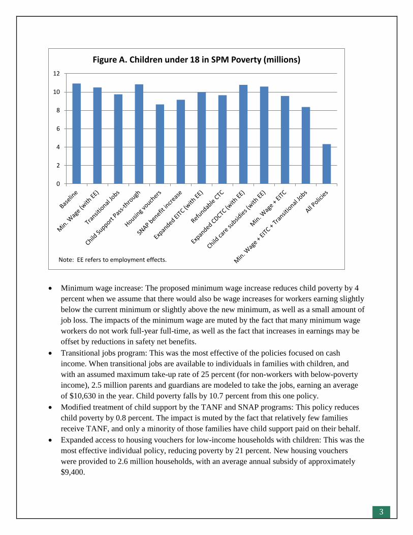
The individual policies had varying impacts on child poverty (figure A).
3
Minimum wage increase: The proposed minimum wage increase reduces child poverty by 4
percent when we assume that there would also be wage increases for workers earning slightly
below the current minimum or slightly above the new minimum, as well as a small amount of
job loss. The impacts of the minimum wage are muted by the fact that many minimum wage
workers do not work full-year full-time, as well as the fact that increases in earnings may be
offset by reductions in safety net benefits.
Transitional jobs program: This was the most effective of the policies focused on cash
income. When transitional jobs are available to individuals in families with children, and
with an assumed maximum take-up rate of 25 percent (for non-workers with below-poverty
income), 2.5 million parents and guardians are modeled to take the jobs, earning an average
of $10,630 in the year. Child poverty falls by 10.7 percent from this one policy.
Modified treatment of child support by the TANF and SNAP programs: This policy reduces
child poverty by 0.8 percent. The impact is muted by the fact that relatively few families
receive TANF, and only a minority of those families have child support paid on their behalf.
Expanded access to housing vouchers for low-income households with children: This was the
most effective individual policy, reducing poverty by 21 percent. New housing vouchers
were provided to 2.6 million households, with an average annual subsidy of approximately
$9,400.
0
2
4
6
8
10
12
Figure A. Children under 18 in SPM Poverty (millions)
Note: EE refers to employment effects.
4
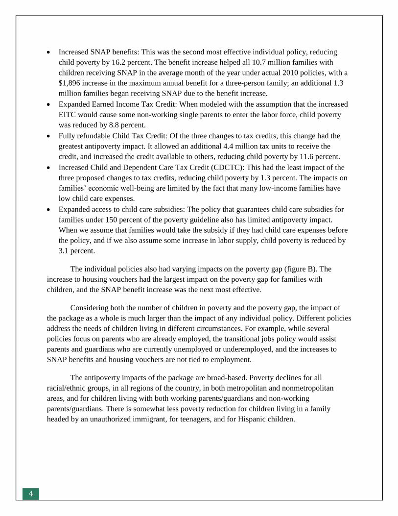
Increased SNAP benefits: This was the second most effective individual policy, reducing
child poverty by 16.2 percent. The benefit increase helped all 10.7 million families with
children receiving SNAP in the average month of the year under actual 2010 policies, with a
$1,896 increase in the maximum annual benefit for a three-person family; an additional 1.3
million families began receiving SNAP due to the benefit increase.
Expanded Earned Income Tax Credit: When modeled with the assumption that the increased
EITC would cause some non-working single parents to enter the labor force, child poverty
was reduced by 8.8 percent.
Fully refundable Child Tax Credit: Of the three changes to tax credits, this change had the
greatest antipoverty impact. It allowed an additional 4.4 million tax units to receive the
credit, and increased the credit available to others, reducing child poverty by 11.6 percent.
Increased Child and Dependent Care Tax Credit (CDCTC): This had the least impact of the
three proposed changes to tax credits, reducing child poverty by 1.3 percent. The impacts on
families’ economic well-being are limited by the fact that many low-income families have
low child care expenses.
Expanded access to child care subsidies: The policy that guarantees child care subsidies for
families under 150 percent of the poverty guideline also has limited antipoverty impact.
When we assume that families would take the subsidy if they had child care expenses before
the policy, and if we also assume some increase in labor supply, child poverty is reduced by
3.1 percent.
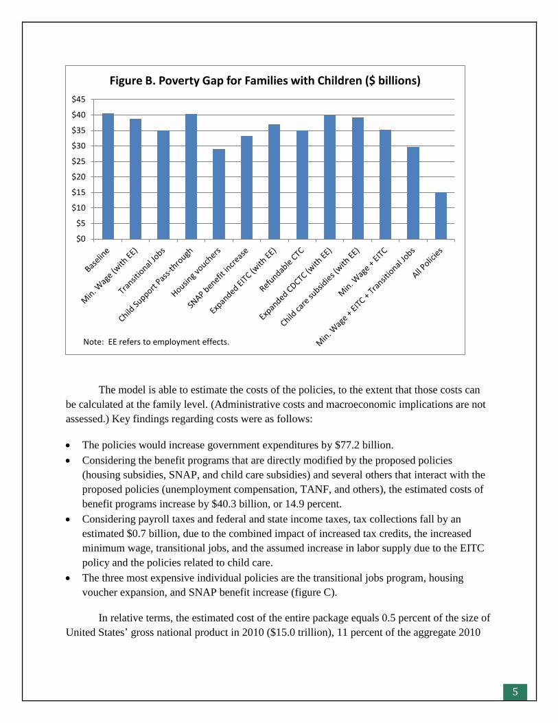
The individual policies also had varying impacts on the poverty gap (figure B). The
increase to housing vouchers had the largest impact on the poverty gap for families with
children, and the SNAP benefit increase was the next most effective.
Considering both the number of children in poverty and the poverty gap, the impact of
the package as a whole is much larger than the impact of any individual policy. Different policies
address the needs of children living in different circumstances. For example, while several
policies focus on parents who are already employed, the transitional jobs policy would assist
parents and guardians who are currently unemployed or underemployed, and the increases to
SNAP benefits and housing vouchers are not tied to employment.
The antipoverty impacts of the package are broad-based. Poverty declines for all
racial/ethnic groups, in all regions of the country, in both metropolitan and nonmetropolitan
areas, and for children living with both working parents/guardians and non-working
parents/guardians. There is somewhat less poverty reduction for children living in a family
headed by an unauthorized immigrant, for teenagers, and for Hispanic children.
5
The model is able to estimate the costs of the policies, to the extent that those costs can
be calculated at the family level. (Administrative costs and macroeconomic implications are not
assessed.) Key findings regarding costs were as follows:
The policies would increase government expenditures by $77.2 billion.
Considering the benefit programs that are directly modified by the proposed policies
(housing subsidies, SNAP, and child care subsidies) and several others that interact with the
proposed policies (unemployment compensation, TANF, and others), the estimated costs of
benefit programs increase by $40.3 billion, or 14.9 percent.
Considering payroll taxes and federal and state income taxes, tax collections fall by an
estimated $0.7 billion, due to the combined impact of increased tax credits, the increased
minimum wage, transitional jobs, and the assumed increase in labor supply due to the EITC
policy and the policies related to child care.
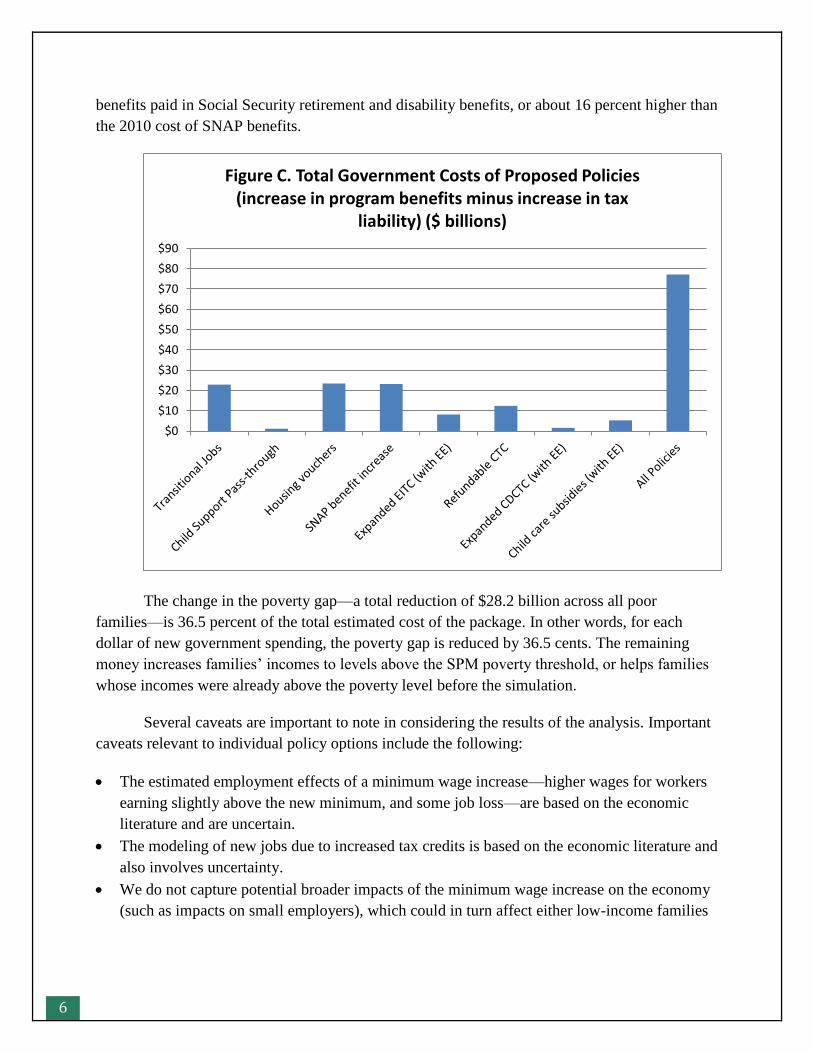
The three most expensive individual policies are the transitional jobs program, housing
voucher expansion, and SNAP benefit increase (figure C).
In relative terms, the estimated cost of the entire package equals 0.5 percent of the size of
United States’ gross national product in 2010 ($15.0 trillion), 11 percent of the aggregate 2010
$0
$5
$10
$15
$20
$25
$30
$35
$40
$45
Figure B. Poverty Gap for Families with Children ($ billions)
Note: EE refers to employment effects.
6
benefits paid in Social Security retirement and disability benefits, or about 16 percent higher than
the 2010 cost of SNAP benefits.
The change in the poverty gap—a total reduction of $28.2 billion across all poor
families—is 36.5 percent of the total estimated cost of the package. In other words, for each
dollar of new government spending, the poverty gap is reduced by 36.5 cents. The remaining
money increases families’ incomes to levels above the SPM poverty threshold, or helps families
whose incomes were already above the poverty level before the simulation.
Several caveats are important to note in considering the results of the analysis. Important
caveats relevant to individual policy options include the following:
The estimated employment effects of a minimum wage increase—higher wages for workers
earning slightly above the new minimum, and some job loss—are based on the economic
literature and are uncertain.
The modeling of new jobs due to increased tax credits is based on the economic literature and
also involves uncertainty.
We do not capture potential broader impacts of the minimum wage increase on the economy
(such as impacts on small employers), which could in turn affect either low-income families
$0
$10
$20
$30
$40
$50
$60
$70
$80
$90
Figure C. Total Government Costs of Proposed Policies (increase in program benefits minus increase in tax
liability) ($ billions)

7
or government tax collections, nor do we capture the potential broader economic impacts of
increased labor supply.
In modeling the policies related to child support income, we do not capture the fact that some
noncustodial parents might increase their child support payments if they knew that their
children would be able to retain those benefits. Also, the estimates capture the effect of
passing through and disregarding currently due child support. Additional antipoverty effects
would be achieved if all past due support (arrears) were distributed to current and former
welfare recipients.
Other important caveats apply to the analysis as a whole, as follows:
The analysis is based on data representing the population, economy, and policies in 2010; the
relative impacts of policies would be different today.
We do not incorporate into the model how the new programs would be paid for. Different
approaches could affect families’ economic well-being in various ways. For example, if new
programs were paid for by reducing spending on existing programs or by altering the tax
system in some way, this could have direct impacts on the economic well-being of some low-
income families.
In the longer run, reductions in poverty for today’s children could have benefits on their
education, health, and employment as young adults and as parents, which could reduce future
poverty levels.
Despite the caveats, the analysis shows the potential for a comprehensive package of
policies to greatly reduce the child poverty rate, and to improve the economic circumstances of
almost all poor children.
8
Introduction
Approximately one in five American children live in families that face substantial economic
hardship. The exact numbers vary by methodology, with the most recent official poverty
statistics counting 22.3 percent of the under-18 population as poor in 2012. The Census Bureau’s
Supplemental Poverty Measure (SPM), which considers the impacts of in-kind benefits and
taxes, shows 18.0 percent as poor in 2012 (Short 2013). Research also shows that children’s
economic hardship would be even greater without the current safety net. For example, Short
(2013) estimates that the SPM poverty rate for families with children would be 24.7 percent
instead of 18 percent in the absence of refundable tax credits. However, even with the current
safety net, and regardless of methodology, the child poverty rate is high, and after falling during
the 1990s, the rate has generally risen over the last decade (Fox, Garfinkel, Kaushal, Waldfogel,
and Wimer, 2014). In the long term, reductions in child poverty could come from improvements
in the economy and in education—leading to higher incomes for the next generation of parents.
But to alleviate economic hardship for today’s children, analysts have proposed more focused
approaches, including changes to taxes and benefit programs.
The research described in this report examines the potential impacts of a set of
antipoverty policies proposed by the Children’s Defense Fund (CDF). The policies include a
minimum wage increase, a transitional jobs program, expanded tax credits, increased availability
of housing and child care subsidies, increased nutrition benefits, and changes to how benefit
programs treat families’ child support income. Using the technique of microsimulation, we
estimated the extent to which the policies would reduce child poverty as well as how much the
policies would cost, for each policy individually and for the package of policies. Poverty was
assessed using the SPM, since that measure takes into account not only a family’s cash income,
but also the value of the in-kind benefits that they receive and the amount of tax that they must
pay.
In addition to capturing the direct impacts of each policy, the analysis incorporates
interactions across policies and programs, such as the fact that a minimum wage increase would
reduce spending on government benefits, while a transitional jobs program would create
increased eligibility for child care subsidies. The analysis also incorporates some potential
behavioral impacts, including the possibility of job loss from a minimum wage increase and the
possibility of increased employment due to newly available child care subsidies.
However, three key limitations of the analysis should be kept in mind. First, the analysis
is based on data for 2010, when the population, economy, and policy rules all differed somewhat
from today. We did not perform any type of “aging” of either the population or the economic
9
circumstances, and we generally left policy rules at their 2010 settings. Thus, we estimate the
potential impacts of the policies if they had been in effect in 2010. The specific costs and
antipoverty impacts of each policy described here would be somewhat different in a different
year. Second, the analysis does not incorporate any method of paying for the policies through
new taxes, reductions in spending, or other policy changes. Different approaches to pay for new
policies could have either direct impacts on low-income families (if a different benefit is
reduced), or secondary impacts (by affecting the economy in a way that affects employment or
prices). Third, the analysis does not capture potential long-run benefits. Reducing the economic
hardship of today’s children could improve their economic circumstances as adults, but that is
not captured in the analysis.
In the discussion below, we first describe the data and methods that we used to estimate
the costs and antipoverty impacts of the CDF policy package. Next, we present information on
the “baseline” level of child poverty in 2010, overall and for different subgroups of children.
This is followed by the core of the report—a discussion of each of the CDF policy proposals. For
each proposal, we present the proposal, describe how we operationalized the proposal in the
context of the microsimulation model, and present the results. After presenting the results of each
policy individually, we show the results that are obtained when the policies are combined. Three
appendices provide additional information. Appendix A compares the simulation model’s
baseline data to actual figures; appendix B assesses the poverty impacts of selected policies that
were in place in 2010 but that have since expired; and appendix C provides very detailed
simulation results, beyond what is presented in the body of the report.
Data and Simulation Methods
The estimates presented in this report are obtained by applying a comprehensive microsimulation
model—the Transfer Income Model, version 3, or TRIM3—to data from the Census Bureau’s
Current Population Survey, Annual Social and Economic Supplement (CPS-ASEC) describing
families’ economic circumstances during 2010. TRIM3’s computer code applies the rules of
government tax and benefit programs to each of the households in the survey data, either
mimicking their real-world operations or simulating hypothetical policy changes. While the CPS-
ASEC contains a wealth of information on families’ demographic characteristics, economic
circumstances, and receipt of government benefits, some information needed for poverty analysis
is missing or inadequate; the TRIM3 model adjusts the data before the simulation of the policy
options. Below, we provide more details on the survey data, the TRIM3 model, the use of
microsimulation to augment the survey data, and the general approach for modeling the
alternative policies.
10
The Current Population Survey
The CPS-ASEC data used in this analysis were collected primarily in spring 2011, and capture
individuals’ incomes and employment during calendar year (CY) 2010. At the point this analysis
was begun, the CY 2010 TRIM-adjusted CPS data were the most recent available for use.1 This
is the same data file that produced the official poverty statistics for 2010, showing that 22
percent of children were living in poverty in 2010 (US Census Bureau 2011b).
The CPS-ASEC is well suited for this analysis for two reasons. First, the sample is
sufficiently large to provide information not only for children overall but also for subgroups of
children with different characteristics: living with single parents versus two parents, in different
racial/ethnic groups, and so on. The file includes information on about 204,983 people in 75,188
households. The Census Bureau attaches “weights” to each person, such that the weighted
sample adds up to the entire civilian noninstitutional population at the time of the survey (306
million people in 119 million households).
Second, the CPS-ASEC includes a wealth of information on the demographic
characteristics and economic circumstances of US households—information that is needed to
apply the antipoverty policies and to assess their impacts. There is detailed information on
individuals’ demographic characteristics and their relationships to other household members, and
extensive information on each adult’s employment and earnings during the year. The survey also
includes information about many types of unearned income, including safety net benefits—
Supplemental Security Income (SSI) and cash assistance from Temporary Assistance for Needy
Families (TANF)—as well as unemployment compensation, workers compensation, veterans’
benefits, retirement and disability benefits, and investment income. Noncash resources covered
by the survey include public housing, other housing assistance, the Supplemental Nutrition
Assistance Program (SNAP, formerly food stamps), the Low Income Home Energy Assistance
Program (LIHEAP), and the Special Supplemental Nutrition Program for Women, Infants, and
Children (WIC). The survey also includes information on households’ work-related child care
expenses.
However, the CPS-ASEC does have some limitations for analysis of families’ economic
resources. One limitation is that there is substantial underreporting of both cash and noncash
benefits. For example, comparison with actual program totals shows that the CPS-ASEC data for
CY 2010 captured about 60 percent of actual TANF benefits and about 56 percent of actual
SNAP benefits.2 Also, the CPS-ASEC does not ask respondents about the amount that they paid
in taxes or received as a tax refund. These limitations are addressed through the TRIM3
1 See US Census Bureau (2011a), for technical documentation of the CPS-ASEC data collected spring 2011.
2 Authors’ tabulations of public-use CPS-ASEC data compared with administrative data on the TANF caseload and
the noninstitutional SSI caseload.

11
“baseline” simulation process, which augments the underreported information and adds in the
missing information, as discussed below. The augmented data can then be used as the foundation
for the analysis of policy options. Another limitation of the CPS-ASEC, not addressed in this
analysis, is that it includes only the noninstitutional population. Thus, US children who are in
institutions—homeless shelters, juvenile detention facilities, or residential programs for children
with special needs—are not included in the analysis.
The TRIM3 Model and the Resources of US Families at the
Baseline
TRIM3 is a comprehensive microsimulation model of the tax and benefit programs affecting US
households. The model is developed and maintained by staff at the Urban Institute with funding
primarily from the Department of Health and Human Services, Office of the Assistant Secretary
for Planning and Evaluation (HHS/ASPE).3 TRIM has been used for over 40 years to assess the
current operation of the US safety net and to estimate the potential impacts of policy changes.
(Full documentation of TRIM3 is available on the project’s website, http://trim3.urban.org.)
Below, we summarize the procedures used to develop the baseline data for this analysis. We then
touch on the changes in the economy and in policies since the year represented by the input data,
and the implications of those changes for the analysis.
The TRIM3 Simulations of Benefits and Taxes
The starting point for this analysis is a version of the CY 2010 CPS-ASEC data that was
previously augmented by Urban Institute staff to create a richer view of families’ resources and
program participation under actual 2010 policies.4 For each of the households in the CPS-ASEC
data, TRIM was used to simulate the major benefit and tax programs, creating new items of
information for each household telling if they are eligible for various programs, their level of tax
liability, and so on. The simulations follow the same steps that an individual would use to
compute his or her income taxes or that a caseworker would use to determine a family’s
eligibility for benefits. For example, TRIM3’s simulation of TANF benefits includes state-
specific variations in income eligibility tests, income disregards, assets tests, and benefit
computation. Furthermore, benefit programs are modeled on a month-by-month basis, capturing
the fact that a family with part-year work might be eligible for different benefits during months
of employment than during months of unemployment. The simulations are described briefly here
and in more detail in TRIM3 technical documentation, available on the project’s website at
3 HHS/ASPE holds the copyright to the CPS version of the model—which is used for this analysis—but allows the
model to be used for other projects.
4 A set of 2010 baseline simulations was previously created under contract with HHS/ASPE. The simulations for
this analysis are slightly modified, incorporating recent enhancements to methods.
12
http://trim.urban.org. Appendix A compares the simulated amounts of taxes and benefits with
program administrative data.
The TRIM-adjusted data file includes some elements that augment information that is
available in the CPS-ASEC survey and other elements that are entirely imputed using TRIM3.
Two types of survey-reported cash income amounts—SSI and TANF—are augmented by the
modeling to adjust for underreporting. For each program, the TRIM3 simulation first identifies
whether each individual and family in the data appears eligible for the program. Eligible
individuals and families that report receiving the benefit are assumed to have reported correctly.
Then, the model selects a portion of the apparently eligible individuals and families that did not
report the benefit to represent the unidentified recipients. For each program, the selection is made
in such a way that the size and key characteristics of the simulated caseload comes acceptably
close to the size and characteristics of the actual caseload. The model also simulates potential
and actual benefit amounts consistent with a family’s survey-reported income and demographic
characteristics.
Similarly, TRIM3 was used to augment the CY 2010 survey-reported data for four in-
kind benefit programs: SNAP, WIC, LIHEAP, and public and subsidized housing. In simulating
SNAP, WIC, and LIHEAP, the model identifies the eligible population, computes potential
benefits, and augments the survey-reported receipt to reach actual caseload levels.5 The
simulation of public and subsidized housing assumes that all current beneficiaries do report their
status in the survey; however, the simulation computes the rental payments that assisted
households are required to pay and uses assumptions about the full value of their apartments to
estimate the value of the subsidy.
TRIM3 also models one additional in-kind program—child care subsidies funded through
the Child Care and Development Fund (CCDF)—for which there is no information in the CPS-
ASEC data. TRIM3 simulates eligibility for CCDF-funded child care subsidies using state-
specific policies and selects a portion of the eligible families as CCDF enrollees in order to come
close to the number and characteristics of actual subsidy recipients. The model also computes
each subsidized family’s copayment.
The CPS-ASEC does not ask respondents any questions about their taxes, but that
information is needed to compute the expanded poverty measure (discussed in more detail
below).6 The simulation computes three kinds of taxes: payroll taxes, federal income taxes, and
5 The WIC simulation does not include eligibility or benefits for pregnant women, since pregnancy is not reported in
the survey and is not imputed in this analysis.
6 The public use version of the CPS-ASEC file includes tax liability amounts that have been imputed onto the file
through Census Bureau procedures. However, for this analysis, it is important that the baseline tax liability amounts
are computed through TRIM3’s procedures, for consistency with the TRIM3-estimated tax liability amounts under
the alternative policy assumptions.
13
state income taxes. The simulation of both federal and state income taxes includes estimation of
tax credit amounts.
All of the simulations and adjustments are internally consistent. For example, if a family
is simulated to receive TANF, the simulated TANF amount is used by the SNAP simulation in
computing a family’s eligibility for SNAP and the level of their SNAP benefit. This internal
consistency allows the estimation of the secondary impacts of policy changes.
One additional aspect of the simulations that is important to note is the treatment of
noncitizens. The CPS-ASEC survey asks respondents to report their citizenship status, country of
origin, and year of entry. However, a noncitizen’s eligibility for benefit programs depends in part
on immigrant status—whether the person is a refugee/asylee, legal permanent resident (LPR),
temporary resident (nonimmigrant), or unauthorized immigrant. Since immigrant status is not
reported in the CPS-ASEC but is important to eligibility determination, procedures are applied as
part of the baseline modeling to impute immigrant status in such a way that the imputed number
of immigrants of each type is consistent with independently derived estimates.7 The simulations
then use the imputed immigrant status information in determining whether an individual is
potentially eligible for a government benefit. In particular, unauthorized immigrants are not
themselves eligible for most government benefits, although families including both unauthorized
and authorized immigrants may receive help.
The result of the TRIM3 simulations is a data file that comes as close as feasible to
capturing the real-world levels of benefits and taxes in 2010. In many cases, the simulations
produce figures that are very close to the actual figures reported in administrative data. For
example, simulated caseloads for SSI, TANF, SNAP, LIHEAP, and WIC all come within 1
percent of administrative targets. The most substantial deviation from targets is in the modeling
of the federal Earned Income Tax Credit (EITC). The simulation identifies only 20.2 million tax
units apparently eligible for the EITC, falling 26 percent short of the total 27.4 million units who
benefitted from the EITC on their 2010 tax return. In general, however, the TRIM3 simulations
bring income and expenses into close alignment with available administrative data for 2010.
(Appendix table A1 shows the simulated data for each benefit and tax program compared to the
administrative targets for that program.)
Changes since 2010
Since 2010, there have been changes in the US population, the economy, and in government
policies. One key difference since 2010 is in the overall health of the economy. The
unemployment rate in 2010 was 9.6 percent, but the 2013 average unemployment rate was 7.4
percent, and the unemployment rate at the start of 2014 was 6.6 percent. However, the drop in
unemployment has not had a substantial impact on child poverty. The official poverty rate for
7 See Passel (2006).
14
children was 22.0 percent in 2010 and had fallen only slightly, to 21.8 percent, in 2012 (the most
recent year of official poverty data available).
Another change since 2010 is in the level of the minimum wage for some workers. The
federal minimum wage is unchanged since 2010, at $7.25. However, between 2010 and early
2014, 14 states increased their state-level minimum wage in nominal terms; about half of those
increases kept pace with inflation but did not result in real increases. The largest increase was in
New Jersey, which used the $7.25 federal minimum in 2010 but is now requiring a minimum
wage of $8.25.8
There have been at least some changes in policies for all of the tax and benefit programs
that affect the SPM computation. Some of those differences:
The temporary increase in SNAP benefits that was funded as a response to the Great
Recession was allowed to expire in November 2013.
The Making Work Pay credit, also instituted in response to the recession, was in place only
in 2009 and 2010.
In many states, there have either been no nominal changes in TANF benefit levels or SSI
state supplements since 2010, or the changes have not kept pace with inflation, meaning that
the real value of those benefits has fallen.
Some states changed aspects of their state income tax systems—such as modifying tax rates
or adding a tax credit—between 2010 and 2014.
The US population has also changed since 2010. The population is slightly larger than it
was in 2010, increasing from 308.7 million as of the 2010 decennial census to an estimated 316.1
million in mid-2013.9 As an example of changes in population characteristics, the portion of the
population identifying as Hispanic was 16.1 percent in spring 2010 but had risen to 17.0 percent
by spring 2012.10
Because of all these differences, the impact of imposing a policy change now could be
somewhat different than the impact of imposing that change in 2010, in terms of the reduction in
child poverty and/or in terms of the cost of the policy. However, creating a baseline file that
attempts to more closely mimic the 2014 population, economic circumstances, and policy
environment was outside the scope of this project. Instead, all of the policies are assessed as if
they had been implemented in 2010, with only one adjustment made to the 2010 “baseline”
environment. That adjustment was to estimate federal income taxes without the Making Work
Pay tax credit. We viewed the Making Work Pay tax credit as a special case for two reasons:
8 See http://www.dol.gov/whd/state/stateMinWageHis.htm and http://www.dol.gov/whd/minwage/america.htm.
9 Figure from the Census Bureau’s national population estimates, vintage 2013.
10 See population data on the Census Bureau website, http://www.census.gov/population/hispanic/ .
15
First, it was only in place in two years and there was never any discussion of extending it beyond
the deep recession period. (In contrast, at the point this project began, the possibility of allowing
SNAP benefits to remain at the increased level was still being discussed.) Second, the fact that
the Making Work Pay Credit was available to virtually all lower- and middle-income employed
taxpayers, and its substantial value ($400 for single individuals, $800 for couples), meant that it
had a noticeable impact on the measured SPM child poverty rate (as shown later in this report).
The other policies related to the recession—such as the SNAP benefit increase and
stimulus provisions related to unemployment benefits—are included in the baseline data, despite
the fact that some of these provisions have since expired. If those policies had not been in place
in 2010, poverty would have been higher (as shown in appendix B). In the absence of the ARRA
policies, the absolute poverty counts, poverty gaps, and poverty rates described in this analysis
would all have been somewhat higher. The relative antipoverty impacts might also differ from
the results that we find when the baseline includes the ARRA policies.
Simulation of Alternative Policies
This project estimates the degree to which alternative policies might alleviate child poverty,
using the baseline data described above as the starting point. The TRIM3 model is used to apply
the desired policy—either a new program or a change in an existing program—to each household
in the survey data. The model determines not only the direct impact of the change—for example,
new earnings from a transitional job, or a higher SNAP benefit—but also picks up other impacts,
on programs and on behavior.
TRIM3 captures the key secondary impacts that a policy change can have on tax and
benefit programs. For example, if a parent receives higher earnings due to an increase in the
minimum wage, the family could potentially receive a lower TANF benefit and/or a lower SNAP
benefit; could have to pay higher contributions toward subsidized housing or subsidized child
care; would owe higher payroll tax; and might see a change in income tax liability. The model
captures secondary impacts on the following benefits and taxes: SSI, TANF, child care subsidies,
housing subsidies, SNAP, LIHEAP, WIC, payroll taxes, federal income taxes, state income
taxes, and unemployment benefits.11 Note that although LIHEAP, WIC, TANF, and child care
subsidies operate with fixed budgets, we did not attempt to recalibrate caseloads or benefits to
hold spending constant.
While the model captures all the key changes in program eligibility, benefit levels, and
taxes, we generally assume that a family’s behavior stays constant across the simulations. In
particular, we generally assume that there are no changes in a family’s decision about whether or
11 We do not estimate any children to lose eligibility for free or reduced-price school meals; in most cases, a child’s
eligibility is in place for the entire school year even if a parent’s earnings increase.
16
not to participate in a government benefit program. In reality, an increase in income (due, for
example, to a minimum wage increase) causes some families that are receiving benefits from
SNAP, TANF, or other programs to be eligible for lower benefits from those programs, which
could cause some of those families to stop participating. Research consistently shows that
families are more likely to participate when they are eligible for a larger benefit (Eslami and
Cunnyngham 2014); however, whether a family already receiving a benefit will drop the benefit
when the value falls probably depends in part on the complexity of the recertification procedures.
Despite the real-world possibility of a change in a decision to participate in a program,
simulating such changes would complicate the interpretation of results. Thus, in most cases, the
simulations assume that families that are eligible both before and after a policy change make the
same decision in both scenarios. However, changes in the SNAP participation decision are
included when we model higher SNAP benefits, and we allow some increase in TANF and
SNAP participation among previously eligible families due to changes in the treatment of child
support income.
The modeling also assumes that family decisions regarding housing and child care
arrangements generally stay constant. Like the assumption of constant program participation
behavior, this assumption is important so that the results of a policy change on a family’s
economic well-being are not complicated by behavioral changes. Of course, for a family with a
housing subsidy or child care subsidy, the required rental payment or copayment could change
due to a change in income, and those changes are picked up by the simulations. Also, in
simulations that model some parents to begin new jobs, a subset of those new workers may be
modeled to begin paying for child care.
Two other categories of expenses—out-of-pocket medical expenses and child support
payments—are treated as constant across the simulations not for conceptual reasons but for
technical reasons. In reality, a family could change its medical spending in response to an
income change, or due to changing health insurance plans after taking a new job; however, the
model is not programmed to estimate changes in out-of-pocket health spending. Finally, we are
not able to estimate how income or employment changes could affect a noncustodial parent’s
payment of child support. In reality, if a noncustodial parent earns more money, he or she might
pay additional child support, increasing the resources of the family where the children reside.
A final type of behavioral question is whether a policy change might induce a person who
is currently not working to begin to work. In general, we would expect that if the benefits of
working increase—due to higher wage-related tax credits or lower out-of-pocket child care
expenses—some individuals who are not currently working might start to work. For this
analysis, policies that would be expected to increase the number of workers are simulated both
with and without those impacts. We rely on the economic literature to suggest the likely
employment impacts, and we then use capabilities within TRIM3 to select specific individuals as
the new workers. Those individuals are assigned a job, and the tax and benefit simulations are
17
then rerun using the newly assigned earnings in determining tax and benefit amounts. Note that
there is substantial uncertainty in predicting the change in employment due to a particular policy
change; further, our methods do not account for the dynamic impacts of increases in labor supply
on wages and prices in the economy.
Child Poverty in 2010
The Importance of Using the SPM
The metric used to estimate the impacts of the alternative policies is the Supplemental Poverty
Measure, or SPM. The US Census Bureau and the Bureau of Labor Statistics developed the SPM
to provide an “improved understanding of the economic well-being of American families and of
how Federal policies affect those living in poverty” (US Census Bureau 2010), building on
earlier work by a panel convened by the National Research Council (Citro and Michael 1995).12
Relative to the official measure of poverty, the SPM uses an expanded definition of resources
and also a different approach to determining poverty thresholds. While numerous variations of
expanded poverty measures have been used since the initial National Research Council analysis,
we use the 2010 research version of the SPM as closely as possible for this analysis (see Short
2011).
The SPM provides a more complete picture of child poverty than the official measure.
Many of the government benefits directed largely or wholly at families with children—such as
the EITC, the WIC program, and child care subsidies—have no impact on the official poverty
measure, but their impact is captured by the SPM’s broader resource measure, which includes
noncash benefits, taxes, work expenses, and medical out-of-pocket expenses, as well as cash
income. While 22.5 percent of US children were estimated to be living in poverty in 2010
according to the official measure, the estimate with the SPM was lower, at 18.2 percent (Short
2011).13 Recent research found that government programs in 2012 reduced child poverty by 12
percentage points and deep child poverty (children with family income less than half of the
poverty level) by 11 percentage points, further emphasizing the importance of capturing these
12 The essential elements of the SPM were originally developed by the National Academy of Sciences’ (NAS) Panel
on Poverty and Family Assistance and published in 1995 (Citro and Michael 1995). Subsequently, the Census
Bureau conducted and published numerous refinements of the measure. In 2009, the Office of Management and
Budget formed an Interagency Technical Working Group that provided recommendations for the development of the
SPM, drawing from the NAS report and incorporating lessons from subsequent research (US Census Bureau 2010).
13 The estimate of 22.5 percent for the official child poverty measure given here is from Short 2011, and includes
unrelated children in the universe. The generally cited figure of 22.0 percent for child poverty in 2010 does not
include children who are unrelated to the household head.
18
resources (Fox et. al. 2014). While the official poverty measure only captures a family as moving
up or down the poverty scale if the family’s cash income changes, the SPM is sensitive to all of
the different policy changes being assessed in this project, thereby allowing us to use a single
metric to compare and contrast the policies’ impacts.
Of course, SPM is a measure of economic well-being, not a complete measure of overall
family well-being. For example, a family’s poverty status as measured by the SPM is not
affected by changes in the quality of child care arrangements for the family’s children, only by
changes in the cost that the family pays out-of-pocket for that child care.
The SPM Resource Measure
The SPM’s resource definition—the dollar amount that is compared to the poverty threshold—is
intended to capture the total amount of economic resources that a family can apply toward food,
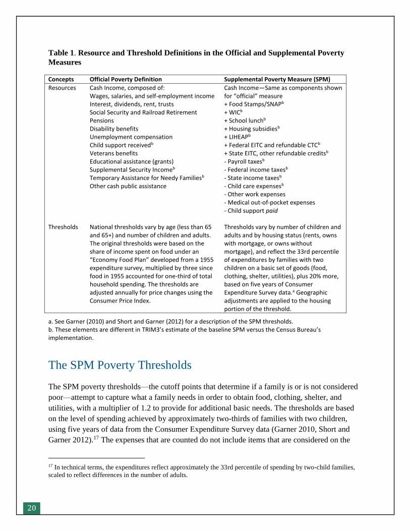
clothing, shelter, and other needs. The components of the measure (table 1) fall into four
categories, as follows:
Cash income: The SPM resource measure starts with the same definition of cash income used
in the official poverty measure. This includes wages; self-employment income; child support;
social insurance income; investment-based income; both government and private retirement
and disability benefits; means-tested cash aid (SSI, TANF, and other cash assistance from the
government); and educational grants. In our implementation of the SPM for this project, most
of these amounts are taken from the CPS-ASEC survey data. However, the SSI and TANF
income components are taken from the TRIM simulation results. Also, for TANF recipients,
child support income amounts are adjusted to reflect only the portion paid to the custodial
parent, and not any amounts retained by the government.
Noncash benefits: The SPM resource measure adds on to a family’s cash income the value of
the noncash benefits that they receive. This includes the value of food assistance (including
SNAP, WIC, and school lunches), the value of living in public or subsidized housing,14 and
the value of LIHEAP benefits. For this analysis, all of these amounts are estimated through
TRIM3 simulation procedures.15 (Note that child care and medical subsidies enter the
resource measure through their impact on nondiscretionary expenses, as discussed below.)
14 The amount of housing subsidy included in the resource measure is capped at the amount of the SPM threshold
considered to be needed for housing (49.7 percent of the total threshold for renters, 51.0 percent for owners with a
mortgage, and 40.4 percent for owners without a mortgage) minus the subsidized household’s required rental
payment.
15 The baseline incidence and value of school meals is estimated by TRIM3; however, as mentioned earlier, the
policy simulations do not capture changes in school meals eligibility, since eligibility often carries over from a prior
school year.
19
Taxes and tax credits: The family’s SPM-defined resources are reduced by the amount that
they pay in payroll tax, federal income tax, and state income tax. However, if the family
benefits from the tax system by qualifying for a refundable tax credit that more than offsets
any positive tax liability, the amount of that net benefit is considered income to the family.
All of the tax and tax credit amounts are simulated, for both the baseline assessment of
poverty and the measurement of poverty under the alternative policy scenarios.
Nondiscretionary expenses: The SPM resource measure subtracts from other resources four
types of nondiscretionary expenditures, reducing what a family can use to meet other needs.
Those expenses are child care expenses, other work-related expenses, medical out-of-pocket
expenses, and child support payments. Child care expenses are reported in the CPS-ASEC,
but TRIM3 augments that information by simulating the receipt of child care subsidies and
calculating the copayments paid by subsidized families; the model also captures changes in
child care expenses due to some of the policy options. Work expenses are imputed by
assuming that each person age 18 and older spends $25.50 on transportation and other work
expenses during each week of work; this assumption is used in the Census Bureau’s SPM
calculations. Both medical out-of-pocket costs and child support payments are taken from the
CPS-ASEC survey.16 Medical expenses and child support payments are not altered in the
simulations of any policy options, although in reality, an individual who takes a new job and
joins an employer’s health insurance plan might face lower or higher out-of-pocket medical
costs as a result; and a nonresident parent who was previously not paying the full amount of a
child support award might begin to do so after taking a new job.
16 The CPS-ASEC identifies an estimated 73 percent of nonresident parents who pay child support and 93 percent of
child support payments. TRIM3 assigns additional nonresident parents to pay child support in order to bring these
totals up to target.
20
Table 1. Resource and Threshold Definitions in the Official and Supplemental Poverty
Measures
Concepts Official Poverty Definition Supplemental Poverty Measure (SPM)
Resources Cash Income, composed of: Wages, salaries, and self-employment income Interest, dividends, rent, trusts Social Security and Railroad Retirement Pensions Disability benefits Unemployment compensation Child support receivedb Veterans benefits Educational assistance (grants) Supplemental Security Incomeb Temporary Assistance for Needy Familiesb Other cash public assistance
Cash Income—Same as components shown for “official” measure + Food Stamps/SNAPb
+ WICb + School lunchb + Housing subsidiesb + LIHEAPb + Federal EITC and refundable CTCb + State EITC, other refundable creditsb - Payroll taxesb - Federal income taxesb - State income taxesb - Child care expensesb - Other work expenses - Medical out-of-pocket expenses - Child support paid
Thresholds National thresholds vary by age (less than 65 and 65+) and number of children and adults. The original thresholds were based on the share of income spent on food under an “Economy Food Plan” developed from a 1955 expenditure survey, multiplied by three since food in 1955 accounted for one-third of total household spending. The thresholds are adjusted annually for price changes using the Consumer Price Index.
Thresholds vary by number of children and adults and by housing status (rents, owns with mortgage, or owns without mortgage), and reflect the 33rd percentile of expenditures by families with two children on a basic set of goods (food, clothing, shelter, utilities), plus 20% more, based on five years of Consumer Expenditure Survey data.a Geographic adjustments are applied to the housing portion of the threshold.
a. See Garner (2010) and Short and Garner (2012) for a description of the SPM thresholds. b. These elements are different in TRIM3’s estimate of the baseline SPM versus the Census Bureau’s implementation.
The SPM Poverty Thresholds
The SPM poverty thresholds—the cutoff points that determine if a family is or is not considered
poor—attempt to capture what a family needs in order to obtain food, clothing, shelter, and
utilities, with a multiplier of 1.2 to provide for additional basic needs. The thresholds are based
on the level of spending achieved by approximately two-thirds of families with two children,
using five years of data from the Consumer Expenditure Survey data (Garner 2010, Short and
Garner 2012).17 The expenses that are counted do not include items that are considered on the
17 In technical terms, the expenditures reflect approximately the 33rd percentile of spending by two-child families,
scaled to reflect differences in the number of adults.
21
resource side of the equation (taxes, child care expenses, or other work expenses), only the items
that a family is assumed to need to buy with its SPM-measured resources.
Note that the SPM poverty thresholds differ markedly from the official poverty
thresholds in both concept and computation. The official thresholds, generally intended to
capture the amount of cash income that a family needs to be nonpoor, were computed in 1963 by
starting from the government’s Economy Food Plan amounts and multiplying by three (since a
third of income was estimated to be spent on food at that time). The official thresholds have been
adjusted for price changes from year to year, but have otherwise been unaltered since their
original development.
The SPM thresholds vary by numerous characteristics. In addition to varying by family
size and number of children (like the official thresholds), the SPM thresholds also vary by
geographic location and by housing tenure. The geographic adjustments are intended to capture
differences in the cost of housing across and within states. The adjustments for housing tenure—
whether a family rents, owns a home with a mortgage, or owns a home without a mortgage—
result in thresholds that are 15.6 percent lower for families that own their home and no longer
have a mortgage compared with otherwise identical households who are renting; thresholds for
those who own their home but still have a mortgage are 2.6 percent higher than for renters,
The differences in concept and computation produce different sets of poverty thresholds.
In 2010, the official poverty threshold was $22,113 for a two-adult, two-child family. The
equivalent SPM thresholds (before adjusting for differences in geographic variation in housing
costs) are $24,391 for a family that rents its home and $25,018 for a family with a mortgage. Of
course, the two sets of thresholds are not directly comparable, since the official thresholds are
intended for comparison with cash income, while the SPM thresholds are intended for
comparison with SPM-defined resource amounts, which may be higher than cash income due to
inclusion of noncash government benefits, or lower than cash income due to inclusion of taxes
and necessary expenses.
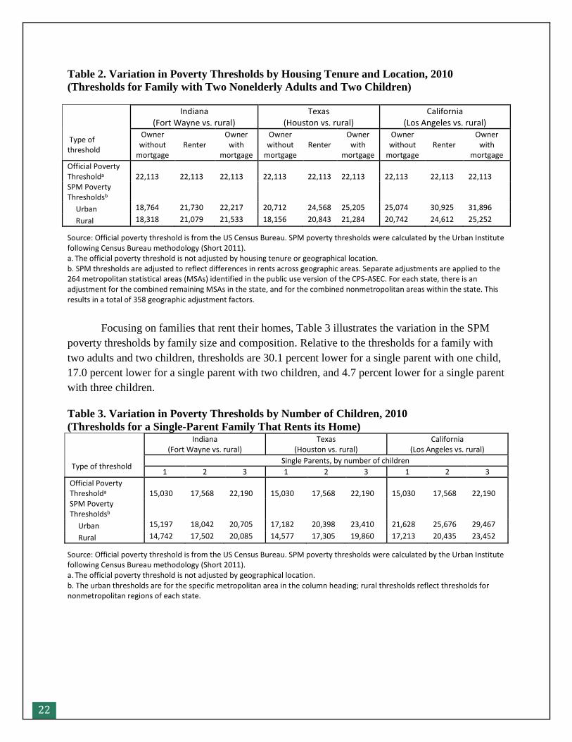
The geographic adjustments can have substantial impacts on the SPM thresholds. For
example, the threshold for a four-person, two-child family that rents its home is $21,730 in Fort
Wayne, Indiana (an area with lower-than-average housing costs), $24,568 in Houston, Texas,
and $30,925 in Los Angeles, California (table 2). The thresholds for nonmetropolitan areas are
generally lower than for metropolitan areas in the same state. For example, the threshold for a
four-person, two-child family that owns its home with a mortgage is $25,205 in Houston,
compared to $21,284 in nonmetropolitan areas of Texas, and $22,217 in Fort Wayne, Indiana,
compared to $21,533 in nonmetropolitan areas of Indiana.
22
Table 2. Variation in Poverty Thresholds by Housing Tenure and Location, 2010
(Thresholds for Family with Two Nonelderly Adults and Two Children)
Indiana
(Fort Wayne vs. rural) Texas
(Houston vs. rural) California
(Los Angeles vs. rural)
Type of threshold
Owner without
mortgage Renter
Owner with
mortgage
Owner without
mortgage Renter
Owner with
mortgage
Owner without
mortgage Renter
Owner with
mortgage
Official Poverty Thresholda 22,113 22,113 22,113 22,113 22,113 22,113 22,113 22,113 22,113 SPM Poverty Thresholdsb
Urban 18,764 21,730 22,217 20,712 24,568 25,205 25,074 30,925 31,896
Rural 18,318 21,079 21,533 18,156 20,843 21,284 20,742 24,612 25,252
Source: Official poverty threshold is from the US Census Bureau. SPM poverty thresholds were calculated by the Urban Institute following Census Bureau methodology (Short 2011). a. The official poverty threshold is not adjusted by housing tenure or geographical location. b. SPM thresholds are adjusted to reflect differences in rents across geographic areas. Separate adjustments are applied to the 264 metropolitan statistical areas (MSAs) identified in the public use version of the CPS-ASEC. For each state, there is an adjustment for the combined remaining MSAs in the state, and for the combined nonmetropolitan areas within the state. This results in a total of 358 geographic adjustment factors.
Focusing on families that rent their homes, Table 3 illustrates the variation in the SPM
poverty thresholds by family size and composition. Relative to the thresholds for a family with
two adults and two children, thresholds are 30.1 percent lower for a single parent with one child,
17.0 percent lower for a single parent with two children, and 4.7 percent lower for a single parent
with three children.
Table 3. Variation in Poverty Thresholds by Number of Children, 2010
(Thresholds for a Single-Parent Family That Rents its Home)
Indiana
(Fort Wayne vs. rural) Texas
(Houston vs. rural) California
(Los Angeles vs. rural)
Type of threshold Single Parents, by number of children
1 2 3 1 2 3 1 2 3
Official Poverty Thresholda 15,030 17,568 22,190 15,030 17,568 22,190 15,030 17,568 22,190 SPM Poverty Thresholdsb
Urban 15,197 18,042 20,705 17,182 20,398 23,410 21,628 25,676 29,467
Rural 14,742 17,502 20,085 14,577 17,305 19,860 17,213 20,435 23,452
Source: Official poverty threshold is from the US Census Bureau. SPM poverty thresholds were calculated by the Urban Institute following Census Bureau methodology (Short 2011). a. The official poverty threshold is not adjusted by geographical location. b. The urban thresholds are for the specific metropolitan area in the column heading; rural thresholds reflect thresholds for nonmetropolitan regions of each state.
23
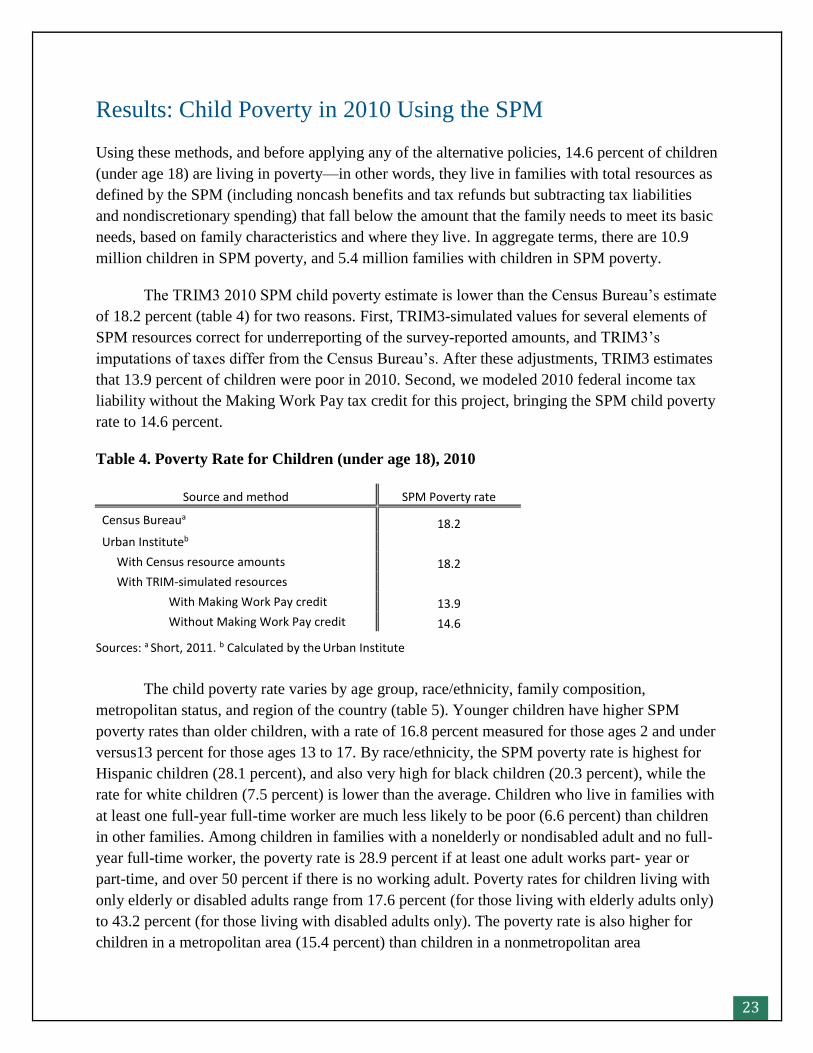
Results: Child Poverty in 2010 Using the SPM
Using these methods, and before applying any of the alternative policies, 14.6 percent of children
(under age 18) are living in poverty—in other words, they live in families with total resources as
defined by the SPM (including noncash benefits and tax refunds but subtracting tax liabilities
and nondiscretionary spending) that fall below the amount that the family needs to meet its basic
needs, based on family characteristics and where they live. In aggregate terms, there are 10.9
million children in SPM poverty, and 5.4 million families with children in SPM poverty.
The TRIM3 2010 SPM child poverty estimate is lower than the Census Bureau’s estimate
of 18.2 percent (table 4) for two reasons. First, TRIM3-simulated values for several elements of
SPM resources correct for underreporting of the survey-reported amounts, and TRIM3’s
imputations of taxes differ from the Census Bureau’s. After these adjustments, TRIM3 estimates
that 13.9 percent of children were poor in 2010. Second, we modeled 2010 federal income tax
liability without the Making Work Pay tax credit for this project, bringing the SPM child poverty
rate to 14.6 percent.
Table 4. Poverty Rate for Children (under age 18), 2010
Source and method SPM Poverty rate
Census Bureaua 18.2
Urban Instituteb
With Census resource amounts 18.2
With TRIM-simulated resources
With Making Work Pay credit 13.9
Without Making Work Pay credit 14.6
Sources: a Short, 2011. b Calculated by the Urban Institute
The child poverty rate varies by age group, race/ethnicity, family composition,
metropolitan status, and region of the country (table 5). Younger children have higher SPM
poverty rates than older children, with a rate of 16.8 percent measured for those ages 2 and under
versus13 percent for those ages 13 to 17. By race/ethnicity, the SPM poverty rate is highest for
Hispanic children (28.1 percent), and also very high for black children (20.3 percent), while the
rate for white children (7.5 percent) is lower than the average. Children who live in families with
at least one full-year full-time worker are much less likely to be poor (6.6 percent) than children
in other families. Among children in families with a nonelderly or nondisabled adult and no full-
year full-time worker, the poverty rate is 28.9 percent if at least one adult works part- year or
part-time, and over 50 percent if there is no working adult. Poverty rates for children living with
only elderly or disabled adults range from 17.6 percent (for those living with elderly adults only)
to 43.2 percent (for those living with disabled adults only). The poverty rate is also higher for
children in a metropolitan area (15.4 percent) than children in a nonmetropolitan area
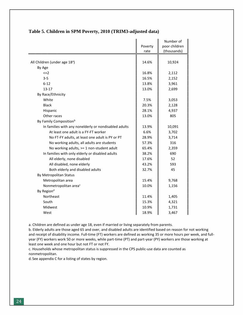
24
Table 5. Children in SPM Poverty, 2010 (TRIM3-adjusted data)
Poverty
rate
Number of poor children (thousands)
All Children (under age 18a) 14.6% 10,924
By Age
<=2 16.8% 2,112
3-5 16.5% 2,152
6-12 13.8% 3,961
13-17 13.0% 2,699
By Race/Ethnicity
White 7.5% 3,053
Black 20.3% 2,128
Hispanic 28.1% 4,937
Other races 13.0% 805
By Family Compositionb
In families with any nonelderly or nondisabled adults 13.9% 10,091
At least one adult is a FY-FT worker 6.6% 3,702
No FT-FY adults, at least one adult is PY or PT 28.9% 3,714
No working adults, all adults are students 57.3% 316
No working adults, >= 1 non-student adult 65.4% 2,359
In families with only elderly or disabled adults 38.2% 690
All elderly, none disabled 17.6% 52
All disabled, none elderly 43.2% 593
Both elderly and disabled adults 32.7% 45
By Metropolitan Status
Metropolitan area 15.4% 9,768
Nonmetropolitan areac 10.0% 1,156
By Regiond
Northeast 11.4% 1,405
South 15.3% 4,321
Midwest 10.9% 1,731
West 18.9% 3,467
a. Children are defined as under age 18, even if married or living separately from parents. b. Elderly adults are those aged 65 and over, and disabled adults are identified based on reason for not working and receipt of disability income. Full-time (FT) workers are defined as working 35 or more hours per week, and full-year (FY) workers work 50 or more weeks, while part-time (PT) and part-year (PY) workers are those working at least one week and one hour but not FT or not FY. c. Households whose metropolitan status is suppressed in the CPS public-use data are counted as nonmetropolitan. d. See appendix C for a listing of states by region.
25
(10.0 percent). By region of the country, SPM poverty rates are higher in the West (18.9 percent)
and South (15.3 percent) than in the Northeast (11.4 percent) or Midwest (10.9 percent).
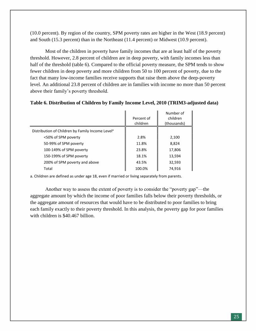
Most of the children in poverty have family incomes that are at least half of the poverty
threshold. However, 2.8 percent of children are in deep poverty, with family incomes less than
half of the threshold (table 6). Compared to the official poverty measure, the SPM tends to show
fewer children in deep poverty and more children from 50 to 100 percent of poverty, due to the
fact that many low-income families receive supports that raise them above the deep-poverty
level. An additional 23.8 percent of children are in families with income no more than 50 percent
above their family’s poverty threshold.
Table 6. Distribution of Children by Family Income Level, 2010 (TRIM3-adjusted data)
Percent of children
Number of children
(thousands)
Distribution of Children by Family Income Levela
<50% of SPM poverty 2.8% 2,100
50-99% of SPM poverty 11.8% 8,824
100-149% of SPM poverty 23.8% 17,806
150-199% of SPM poverty 18.1% 13,594
200% of SPM poverty and above 43.5% 32,593
Total 100.0% 74,916
a. Children are defined as under age 18, even if married or living separately from parents.
Another way to assess the extent of poverty is to consider the “poverty gap”—the
aggregate amount by which the income of poor families falls below their poverty thresholds, or
the aggregate amount of resources that would have to be distributed to poor families to bring
each family exactly to their poverty threshold. In this analysis, the poverty gap for poor families
with children is $40.467 billion.
26
Policy Changes to Reduce Child Poverty
The CDF proposal includes nine policies for reducing child poverty. Three of the policies are
primarily increases to cash income: a higher minimum wage, transitional jobs, and allowing
TANF recipients to retain more child support. Two policies increase in-kind income, by
increasing housing subsidies and SNAP benefits. Three policies reduce income taxes by
increasing the EITC, the Child Tax Credit, and the Child and Dependent Care Tax Credit, and a
final policy reduces work expenses by increasing the availability of child care subsidies. For
each policy change, we describe the general concept, explain how it was implemented within the
simulation model, and present the results. We then present the results of simulations that
combine selected elements of the overall proposal: First combining the EITC increase and
minimum wage increase, and then adding transitional jobs. Next, all nine policies are modeled in
combination. The discussion of each policy includes a table showing key impacts on poverty and
overall impacts on government benefit spending and tax collections. Appendix C shows
additional details on the simulation results, including additional poverty detail, changes for each
benefit and tax program individually, and information on how benefits and taxes change by
family poverty level; the discussion below includes some references to specific appendix tables.
As discussed earlier, all of the policies are modeled with the 2010 population, economy,
and program rules as the starting point. In appendix B, we show the estimated impact on child
poverty of the removal of two policies that were in place in 2010: the temporary SNAP benefit
increase and the expansion of refundable tax credits.
Increasing Cash Income
One of the most direct ways to address poverty is to increase families’ cash incomes; in fact, it is
the only kind of policy that changes resources as defined by the official poverty measure. This
first set of policies provides greater income to families through the labor market or cash
assistance.
Higher Minimum Wage
The first component of the CDF policy package increases the minimum wage to $10.10 per hour
for covered workers, and to 70 percent of that level ($7.07) for tipped workers. These figures
were proposed in the Harkin-Miller Fair Minimum Wage Act of 2013, and President Obama
recently raised the wage for federal contract workers to $10.10. The minimum wage currently
stands at $7.25 nationally, although 21 states and the District of Columbia have higher

27
minimums, with the highest being $9.19 per hour in Washington state.18 The federal minimum
wage has been set at $7.25 since July 2009, and the “subminimum wage” for tipped workers has
been unchanged since 1996, at $2.13.
Methods: Simulating the higher minimum wage involved deflating the desired minimum
wage; identifying workers with wages lower than the new minimum and covered by the law;
increasing the earnings of those workers; and simulating the impact of individuals’ higher wages
on the full range of benefit and tax programs. Also, in one version of the simulation, we modeled
the indirect employment effects of a minimum wage increase.
Since the analysis uses 2010 data and the 2010 poverty thresholds, the $10.10 wage is
deflated from current (2014) dollars to 2010 dollars, lowering the nominal wage to $9.30 per
hour for most workers, and to $6.51 for tipped workers.19 This ensures that the earnings of a full-
time, full-year minimum-wage worker are at approximately the same percentage-of-poverty in
our 2010-based analysis as would be the case if the new minimum wage was implemented in
2014—something that is of key importance for this analysis. For a parent with two children, full-
year full-time wages at $10.10 will equal approximately 110 percent of the official poverty
threshold; likewise, full-year full-time wages at $9.30 equal 110 percent of the 2010 poverty
threshold.20 Note, however, that this means that the percentage increase in the minimum wage is
understated. Specifically, an increase from $7.25 to $10.10 is a 39 percent increase in wages, but
the increase from $7.25 to the deflated value of $9.30 is only a 28 percent increase.
Workers who would benefit from the $10.10 minimum wage ($9.30 when deflated) are
those whose wage is below the new minimum, and who are covered by the policy. For purposes
of the simulation, each worker’s hourly wage is obtained from a combination of information
available in the survey data. For 63 percent of workers, a specific hourly wage is available, and
for the remainder we estimated an hourly wage based on their reported annual earnings, weeks of
work, and hours per week.21 Note that the procedures use a single wage for each individual, and
18 Current and historical data on state minimum wages are provided on the website of the US Department of Labor,
Wage and Hour Division, http://www.dol.gov/whd/minwage/america.htm.
19 To calculate the deflation, we used the Consumer Price Index for all Urban Customers (CPI-U). Since CPI-U
values for 2014 are not yet available, we used the Congressional Budget Office’s CPI-U projections (2014a).
20 Since the 2014 poverty thresholds are not yet available, this computation inflates the 2013 thresholds by the
projected change in the CPI-U.
21 The basic portion of the CPS (as opposed to the annual CPS-ASEC) is conducted monthly, surveying the same
households for four consecutive months. Each month, workers who will not be surveyed in the following month (in
the “outgoing rotation group”) are asked their exact hourly wage at that point in time, which we use for this analysis
when available. For workers in the CPS-ASEC who were not asked their wage, we looked for the data in the CPS
survey in later months when they were asked the question. Some CY 2010 workers were not working at the point
that they were in the outgoing rotation group, did not complete that survey, or their later data could not be matched
for technical reasons. The exactly reported hourly wages are more reliable than computations based on earnings,
weeks, and hours, but have the disadvantage that they may not accurately capture earnings during the calendar year.
See Appendix B of Giannarelli, Morton, and Wheaton (2007), for more discussion.
28
do not capture the real-world complexity that an individual may have changed jobs or worked
multiple jobs during the year. We assume that workers whose hourly wage is more than 5 cents
below the actual minimum wage (less than $7.20 per hour in states with no state minimum, or
more than 5 cents below their state’s minimum wage) must have been in jobs not covered by the
minimum wage law, so their wages are not increased to $9.30. (We allow the 5-cent difference
due to the imprecision when hourly wages are calculated.) Also, individuals who are self-
employed are assumed to be unaffected by the minimum wage increase.22
Tipped workers were identified as those making less than the regular minimum wage23
and working in one of seven occupation groups: waiters/waitresses, bartenders, gaming service
workers, barbers, hairdressers/hairstylists/cosmetologists, massage therapists, and miscellaneous
personal appearance workers. These occupational categories were chosen to correspond to those
used in a recent study of tipped workers (Allegretto and Filion 2011).
An affected worker’s earnings were increased by the ratio of the new minimum wage to
the current hourly wage.24 For example, the earnings of someone making $7.25 per hour in the
baseline data are increased by 28 percent, and the earnings of someone making $9.00 per hour in
the baseline data are increased by 11 percent. The same proportional increase is made to both
annual and monthly earnings. After increasing earnings, the model re-simulates all of the benefit
and tax programs before re-computing the SPM poverty results.
In addition to the required legal impacts of a minimum wage increase—that people
earnings less than the new minimum receive a wage increase—there could be two additional
responses in the labor market. First, there might be some job loss if employers reduce their use of
labor in response to the higher wages. Second, there could be “spillover effects” on the wages of
individuals whose wages would not legally have to be increased. We simulated the policy once
without any spillover effects or job loss, and a second time with those impacts included.
The extent of job loss that would result from a minimum wage increase is uncertain.
Some recent studies have found no impact (such as Schmitt 2013), while among studies that do
find impacts, the probability of losing a job is estimated to range from a few percent of the
22 For individuals with both self-employment and wage and salary earnings, a minimum wage increase could affect
the wage and salary portion of earnings. However, for individuals with both types of earnings for whom hourly
wage data were not available, an hourly wage could be estimated only by assuming the same hourly earnings from
both self-employment and nonself-employment. Because that assumption is unlikely to be true, and since there were
very few low-wage individuals with self-employment earnings in the survey data, we excluded all individuals with
any self-employment income from any wage adjustments.
23 Specifically, the tipped workers targeted were those making from up to 5 cents below each state’s minimum wage
for tipped workers up to 5 cents below the state’s regular minimum wage. Thus, in states where the tipped worker
wage is equal to the regular minimum wage, no tipped workers are identified.
24 If a worker’s current wage is between $7.20 and $7.25, the wage increase is computed assuming that the current
wage is $7.25; and for tipped workers, if the current wage is slightly below the state’s sub-minimum wage, the
state’s sub-minimum is used.
29
percentage change in earnings to about one-quarter of the percentage change in earnings
(Neumark and Wascher 2006). A recent Congressional Budget Office report (2014b, released
after we completed this part of the analysis) assumed that a 10 percent increase in the minimum
wage would result in a 1 percent decline in overall teen employment and a 0.33 percent decline
in overall adult employment. Based on these assumptions, the CBO calculated elasticities for
workers directly affected by the minimum wage increase so as to achieve the overall estimated
employment effect.
For this simulation, we assumed that a worker’s probability of losing his or her job is
equal to 6 percent of the change in wages—the same assumption used for a 2007 TRIM-based
analysis of minimum wage increases (Giannarelli, Morton, and Wheaton 2007). To implement
the assumption, we multiply a worker’s percentage increase in wage by 0.06 to obtain the
probability of losing the job. For example, for a worker earning $7.75/hour in 2010 whose wage
would have to be increased by 20 percent to come up to the new (deflated) minimum of $9.30,
there is a 1.2 percent chance of losing the job. The choice of exactly which workers lose their
jobs involves a random component.25 We did not model different job-loss probabilities for adults
versus teens, and we did not model any reductions in hours of employment. We assume that most
workers imputed to lose their jobs would be eligible for unemployment compensation, and we
compute the amount of compensation based on the policies in their state.
The rationale for modeling spillover effects is that employers might need to maintain
some consistency in relative wage rates for workers earning just below or above the new
minimum wage rates. For example, if Worker A previously earned $9.50 and Worker B earned
$7.25, the employer would be required to raise Worker B’s wages to $9.30, but might also decide
to raise Worker A’s wage somewhat. Likewise, if an employer previously paid $6.50 to a worker
not covered by the minimum wage, the minimum wage increase might induce the employer to
increase that worker’s wage to be closer to the new minimum. In the 2010 data, we assumed that
workers with wages as low as $6.25 and as high as $10.30 would receive proportional wage
adjustments, phasing out to zero at the ends of the distribution. (To simplify the modeling, we
assume that tipped workers are only affected by the spillover effect for all workers.) This is a less
generous spillover assumption than used in recent analysis by Cooper and Hall (2013), making
our estimates a conservative approach.
The analysis does not capture broader potential “ripple effects” of a minimum wage
increase. For example, the owner of a small business who now pays more to his workers might
lower his own salary and so might pay less in taxes. Any increases in prices would have some
impact on the SPM thresholds, since those thresholds are computed using expenditure data. Our
analysis does not capture either of those broader potential impacts.
25 We compare these probabilities to a random number for each affected worker; in the example in the text, if the
random number is below 0.012, the person is simulated to lose their job.
30
Results: When the minimum wage increase is implemented without job loss or spillover
effects, 15.3 million individuals are estimated to obtain a wage increase, with an average
increase in annual earnings of $1,817 (table 7). The total number of workers receiving a wage
increase includes 6.3 million who are in families with children, who see their earnings increase
by an average of $1,709 (table C3.2b). The increase in the minimum wage reduces child poverty
from the baseline level of 14.6 percent to 14.2 percent—a 2.3 percent drop in child poverty. Not
surprisingly, the percentage reduction is larger (4.1 percent) for children in families with full-
year full-time workers, and there is no impact on children in families living with adults who are
out of the labor force. The percentage reduction is larger in the Midwest (4.9 percent), likely due
to a combination of the minimum wage laws in the Midwestern states (only one-third of
Midwestern states have a state minimum higher than the federal) and the number and
characteristics of minimum wage workers in that region. When government programs are
resimulated with the modified earnings, the higher earnings mean that some families are no
longer eligible for certain programs, others are eligible for lower benefits, and families owe more
in taxes. In the aggregate, benefits fall by $1.6 billion, and net taxes increase by $8.5 billion.26
When the job loss and spillover effects are included, 27.6 million workers receive higher
wages, including 11.4 million people in families with children. An estimated 0.3 million
workers, including 0.1 million in families with children, lose their jobs.27 The number of jobs
lost equals 0.2 percent of total employment (there were 153.3 million employed individuals in
2010). In the aggregate, the higher minimum wage with spillover effects and job loss is
estimated to increase the earnings of workers (in families with and without children) by $44.9
billion.
Families with higher wages may become eligible for lower benefits and will generally
owe higher taxes,28 while families with someone who loses a job may become eligible for
unemployment compensation and other benefits, and will owe lower taxes. The benefit programs
with the largest aggregate changes are SNAP (a reduction of $1.6 billion, or 2.4 percent),
unemployment compensation (an increase of $1 billion, or 1 percent), and housing subsidies (a
reduction of $318 million, or 0.9 percent). There are also reductions in SSI benefits, TANF
benefits, child care subsidies, LIHEAP, and WIC. Overall, the cost of benefits falls by $1.5
billion. The overall increase in tax liability is $13.7 billion, with increases of $6.7 billion (0.8
26 The benefits that are considered are unemployment compensation, SSI, TANF (including the impact of TANF on
retained child support), housing and child care subsidies, SNAP, LIHEAP, WIC, and (in later simulations), the costs
of transitional jobs. Taxes include payroll taxes and federal and state income taxes.
27 Table C3.2b shows the workers who gain earnings minus those who lose jobs—27.335 million in total and 11.383
million in families with children.
28 Families with very low earnings that place them in the phase-in range of the EITC may become eligible for a
larger EITC as earnings increase, reducing their net federal income taxes.
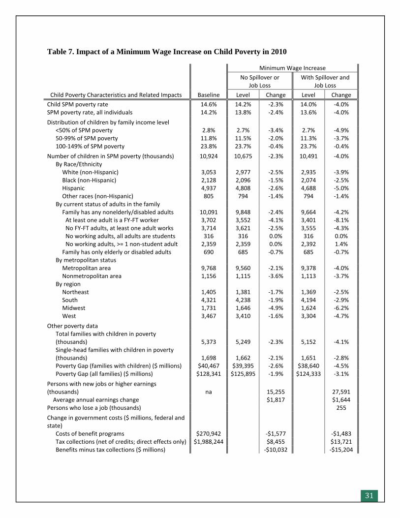
31
Table 7. Impact of a Minimum Wage Increase on Child Poverty in 2010
Baseline
Minimum Wage Increase
Child Poverty Characteristics and Related Impacts
No Spillover or Job Loss
With Spillover and Job Loss
Level Change Level Change
Child SPM poverty rate 14.6% 14.2% -2.3% 14.0% -4.0% SPM poverty rate, all individuals 14.2% 13.8% -2.4% 13.6% -4.0%
Distribution of children by family income level <50% of SPM poverty 2.8% 2.7% -3.4% 2.7% -4.9% 50-99% of SPM poverty 11.8% 11.5% -2.0% 11.3% -3.7% 100-149% of SPM poverty 23.8% 23.7% -0.4% 23.7% -0.4%
Number of children in SPM poverty (thousands) 10,924 10,675 -2.3% 10,491 -4.0% By Race/Ethnicity White (non-Hispanic) 3,053 2,977 -2.5% 2,935 -3.9% Black (non-Hispanic) 2,128 2,096 -1.5% 2,074 -2.5% Hispanic 4,937 4,808 -2.6% 4,688 -5.0% Other races (non-Hispanic) 805 794 -1.4% 794 -1.4% By current status of adults in the family Family has any nonelderly/disabled adults 10,091 9,848 -2.4% 9,664 -4.2% At least one adult is a FY-FT worker 3,702 3,552 -4.1% 3,401 -8.1% No FY-FT adults, at least one adult works 3,714 3,621 -2.5% 3,555 -4.3% No working adults, all adults are students 316 316 0.0% 316 0.0% No working adults, >= 1 non-student adult 2,359 2,359 0.0% 2,392 1.4% Family has only elderly or disabled adults 690 685 -0.7% 685 -0.7% By metropolitan status Metropolitan area 9,768 9,560 -2.1% 9,378 -4.0% Nonmetropolitan area 1,156 1,115 -3.6% 1,113 -3.7% By region Northeast 1,405 1,381 -1.7% 1,369 -2.5% South 4,321 4,238 -1.9% 4,194 -2.9% Midwest 1,731 1,646 -4.9% 1,624 -6.2% West 3,467 3,410 -1.6% 3,304 -4.7%
Other poverty data
Total families with children in poverty (thousands) 5,373 5,249 -2.3% 5,152 -4.1%
Single-head families with children in poverty (thousands) 1,698 1,662 -2.1% 1,651 -2.8%
Poverty Gap (families with children) ($ millions) $40,467 $39,395 -2.6% $38,640 -4.5% Poverty Gap (all families) ($ millions) $128,341 $125,895 -1.9% $124,333 -3.1%
Persons with new jobs or higher earnings (thousands) na 15,255 27,591
Average annual earnings change $1,817 $1,644 Persons who lose a job (thousands) 255
Change in government costs ($ millions, federal and state) Costs of benefit programs $270,942 -$1,577 -$1,483 Tax collections (net of credits; direct effects only) $1,988,244 $8,455 $13,721 Benefits minus tax collections ($ millions) -$10,032 -$15,204
32
percent) in payroll tax (including the employer and employee shares), $5.6 billion (0.7 percent)
in federal income tax, and $1.4 billion (0.6 percent) in state income tax. Combining the
aggregate increase in earnings ($44.9 billion), with the reduction in benefits ($1.5 billion) and
increase in taxes paid by workers ($10.2 billion), the minimum wage increase with job loss and
spillover effects is estimated to add $33.2 billion to families’ resources.
The increase in family resources causes child poverty to fall to 14.0 percent, a 4.0 percent
drop, with a drop of 8.1 percent for children living with a full-time full-year worker. The poverty
gap for families with children—the aggregate amount by which their incomes fall below their
poverty thresholds—falls by $1.8 billion, or 4.5 percent. An increase in the minimum wage also
reduces poverty in families without children. Overall—for individuals of all ages—the minimum
wage increase with the job loss and spillover effects reduces poverty from 14.2 percent to 13.6
percent, and the overall poverty gap is reduced by $4.0 billion, or 3.1 percent.
The relatively modest antipoverty impacts of a minimum wage increase standing alone
are generally consistent with prior TRIM-based analysis (e.g., Giannarelli, Morton, et al. 2007
and Giannarelli, Lippold, et al. 2012). A key factor is that most of the workers who benefit from
a minimum wage increase are in families already above the SPM poverty level. Among the 27.6
million workers with a wage increase when spillover effects are included, 18 percent are in
families with resources below the SPM poverty limit, 45 percent have family resources from 100
to 200 percent of SPM poverty, and 37 percent are in families at 200 percent of the SPM level or
higher. Also, many individuals who earn the minimum wage do not work full-year or do not
work full-time, muting the effect of the wage increase on annual earnings. A number of affected
workers have earnings above the old minimum wage and so receive an increase in hourly
earnings that is smaller than the full difference between the old and new minimum wage. Finally,
the fact that a portion of the new earnings are absorbed by benefit reductions and/or tax increases
somewhat lessens the antipoverty impact.
Transitional Jobs
A second key component of the CDF policy package is a transitional jobs (TJ) program directly
focused on families with children. Specifically, the proposal envisions that publicly funded
transitional jobs will be available to individuals who reside in families that include children
under 18, who are ages 16 to 64, who have a valid Social Security Number for work purposes,
and who are either not working or working 32 or fewer hours per week. The jobs would not be
available to individuals receiving SSI or Social Security income, but they would be available to
individuals with disabilities not receiving either of those benefits, with the assumption that
appropriate employment could be found.29 Note that parents who do not live with their children
29 The jobs are also envisioned to be restricted to nonincarcerated people, although we did not model this restriction,
as the CPS-ASEC universe only includes people living outside of institutions.

33
(noncustodial parents) were not modeled as receiving TJs in the simulation, although they might
be eligible under some program designs.30
The conceptual design assumes that a TJ position would be available for a maximum of
30 weeks, and that an individual would have to look for a non-TJ job for 4 weeks before taking
another TJ job. TJ workers would be able to work 40 hours per week, but could also choose to
take the TJ job as a part-time job. The TJ workers would earn the prevailing minimum wage.
These aspects of the program design are the same as in the TJ program proposed by Community
Advocates Public Policy Institute (Community Advocates Public Policy Institute 2012).
The jobs would be available to anyone who qualified, although it is assumed that not
everyone who qualifies would want to take the job. For example, an unemployed individual who
previously worked for well above the minimum wage and who was able to go without pay while
looking for another position would likely not take the job.
A final key aspect of the proposal is that subsidized child care would be made available
to any TJ worker who desired a subsidy, and who was eligible for subsidies under the standard
CCDF rules in her/his state of residence. Implicitly, this assumes that the TJ program would
include sufficient funding for additional child care subsidies.
Methods: To identify the potential TJ workers, we define families broadly to include all
related persons living in a household; thus, if a grandparent lives with a young-adult daughter
and the daughter’s child, both the parent and the grandparent could be eligible for a TJ. To
capture the SSN requirement, the jobs are not available to individuals who were previously
imputed to be unauthorized immigrants. We assume that individuals taking up a transitional job
will do so for 48 weeks per calendar year—that is working full year but allowing for a 4-week
gap between transitional job spells (as specified by the policy rules). This approach assumes that
no transitional jobs participants will transition into regular (unsubsidized) jobs during the study
period, so gives an upper-bound estimate of the program’s cost.
A key driver of the cost and impact of a TJ program is the assumption about what
percentage of eligible individuals would sign up for the program. The largest federally funded
public service employment programs in recent history, the Comprehensive Employment and
Training Act programs of the 1970s, had approximately a 7 percent take-up rate at their height
(Mirengoff et al. 1980). Similarly, the Job Training Partnership Act of the 1980s, while
providing only job training rather than employment, had less than a 10 percent take-up rate
(Doolittle et al. 1993). Transitional jobs programs provided under TANF emergency funding
during the 2008-2010 recession served no more than 15 percent of eligible individuals; however,
30 Within the scope of this project, it would not have been possible to link an increase in a noncustodial parent’s
income to a change in resources for the custodial family.
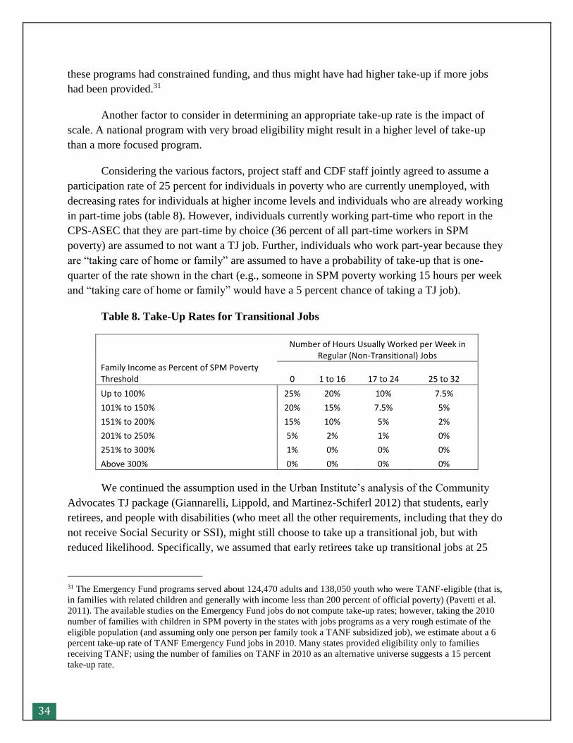
34
these programs had constrained funding, and thus might have had higher take-up if more jobs
had been provided.31
Another factor to consider in determining an appropriate take-up rate is the impact of
scale. A national program with very broad eligibility might result in a higher level of take-up
than a more focused program.
Considering the various factors, project staff and CDF staff jointly agreed to assume a
participation rate of 25 percent for individuals in poverty who are currently unemployed, with
decreasing rates for individuals at higher income levels and individuals who are already working
in part-time jobs (table 8). However, individuals currently working part-time who report in the
CPS-ASEC that they are part-time by choice (36 percent of all part-time workers in SPM
poverty) are assumed to not want a TJ job. Further, individuals who work part-year because they
are “taking care of home or family” are assumed to have a probability of take-up that is one-
quarter of the rate shown in the chart (e.g., someone in SPM poverty working 15 hours per week
and “taking care of home or family” would have a 5 percent chance of taking a TJ job).
Table 8. Take-Up Rates for Transitional Jobs
Number of Hours Usually Worked per Week in
Regular (Non-Transitional) Jobs
Family Income as Percent of SPM Poverty Threshold 0 1 to 16 17 to 24 25 to 32
Up to 100% 25% 20% 10% 7.5%
101% to 150% 20% 15% 7.5% 5%
151% to 200% 15% 10% 5% 2%
201% to 250% 5% 2% 1% 0%
251% to 300% 1% 0% 0% 0%
Above 300% 0% 0% 0% 0%
We continued the assumption used in the Urban Institute’s analysis of the Community
Advocates TJ package (Giannarelli, Lippold, and Martinez-Schiferl 2012) that students, early
retirees, and people with disabilities (who meet all the other requirements, including that they do
not receive Social Security or SSI), might still choose to take up a transitional job, but with
reduced likelihood. Specifically, we assumed that early retirees take up transitional jobs at 25
31 The Emergency Fund programs served about 124,470 adults and 138,050 youth who were TANF-eligible (that is,
in families with related children and generally with income less than 200 percent of official poverty) (Pavetti et al.
2011). The available studies on the Emergency Fund jobs do not compute take-up rates; however, taking the 2010
number of families with children in SPM poverty in the states with jobs programs as a very rough estimate of the
eligible population (and assuming only one person per family took a TANF subsidized job), we estimate about a 6
percent take-up rate of TANF Emergency Fund jobs in 2010. Many states provided eligibility only to families
receiving TANF; using the number of families on TANF in 2010 as an alternative universe suggests a 15 percent
take-up rate.
35
percent of the rate for their poverty and hour categories, students at 50 percent of the standard
rates, and persons with disabilities at 75 percent of the standard rates.
For individuals not working in the baseline who are selected to take a TJ, we assumed
that 56 percent desire full-time jobs (40 hours per week) and 44 percent desire part-time jobs (20
hours per week). That distribution is based on the distribution of full-time and part-time
employment for workers in SPM poverty in the 2010 CPS-ASEC data. For individuals working
part-time in the baseline who are selected to take a TJ, we always increase their hours of work to
40 per week.
After identifying individuals eligible for the TJs, selecting specific recipients (based on
the probabilities described above combined with a random element), and determining desired
hours for new workers, all employment data for the affected individuals were modified to reflect
the new TJ jobs. For a person who did not work at all in the baseline simulation, the amount of
new earnings equals the desired weekly hours (20 or 40) times the federal minimum wage, in
each of 48 weeks. The modified information was then used to re-simulate all the benefit and tax
programs.
As mentioned above, child care subsidies are assumed to be available to any TJ worker
who desires a subsidy, and who is eligible for subsidies under the standard CCDF rules in her/his
state of residence once he or she begins working. (Note that in a two-parent family, both must be
working or in school for the family to be eligible for subsidies.) We assumed that half of the
families that became eligible for CCDF due to the TJ program in the average month of the year
would want to enroll in CCDF. In selecting which newly eligible families would participate, the
probability of participation was based on the same demographic characteristics used to identify
the baseline CCDF enrollment: whether a one-parent or two-parent family, race/ethnicity, lower
or higher income, and ages of children.32 For families with new workers who are assumed to not
take the CCDF subsidy (including those who were not eligible for CCDF), a set of imputation
equations was used to estimate the probability that the family would have positive expenses and,
if so, the level of those expenses.33
Results: Under the participation assumptions discussed above, 2.5 million individuals
who are currently not working or who are working part-time are simulated to take a transitional
job, with an average annual increase in earnings of $10,630 (table 9). Consistent with the
32 The participation probabilities—used in the baseline simulations of CCDF enrollment—are based on a
comparison of TRIM-simulated eligible families with families actually receiving CCDF according to administrative
data. The standard probabilities were adjusted upwards to achieve the desired 50 percent take-up among newly
eligible families.
33 The equations were estimated for a prior project and capture the relative impacts of family income, parents’ work
hours, ages of children, race/ethnicity, and family composition. The equations were calibrated so that, when applied
to the full CPS-ASEC data, they reproduce the same incidence and level of child care expenses as actually reported
in the CPS-ASEC data.
36
program specifications, all the TJ workers are in families with children. The aggregate increase
in earnings for families with children is $26.7 billion—about $9.0 billion more than the earnings
increase for families with children when the minimum wage is increased, including spillover
effects (table C3.2b).
After factoring in the impacts of the new earnings on families’ safety-net benefits and tax
liability, the TJ program reduces the number of children in SPM poverty by 1.2 million, reducing
the SPM child poverty rate from 14.6 percent to 13.0 percent, a drop of 10.7 percent. The
number of families with children in SPM poverty falls by 0.5 million. Compared to the number
of new jobs, it is clear that the TJ jobs do not necessarily raise the families of the new workers
out of poverty. However, there is a substantial impact on the rate of deep poverty, which falls by
18.6 percent. Also, the poverty gap for families with children falls by $5.6 million, or 13.9
percent—a somewhat greater relative impact than the impact on the child poverty rate. (Since the
TJ jobs are available only to families with children, there is no change in the poverty gap for
families without children.)
The TJ policy produces somewhat lower benefits for Hispanic children (an 8.8 percent
reduction in poverty) compared with children of other racial/ethnic groups, with the largest
impacts for black children (a 14.0 percent poverty reduction). The fact that the impacts are lower
for Hispanic families is partly related to the fact that a higher portion of Hispanic adults are
estimated to be unauthorized immigrants compared with adults of other racial/ethnic groups.
Because the policy is designed to include jobs for individuals with disabilities, there is a
7.2 percent reduction in the number of children in poverty who live in families in which all
adults are elderly or have disabilities. Also, the fact that the policy primarily benefits individuals
without jobs means that the number of poor children living with non-working (but nonelderly,
nondisabled) adults falls substantially, by 0.8 million. (Note that many of these children remain
poor in the TJ simulation but are classified as children living with working adults.)
The TJ policy requires substantial government costs. The cost of the wages alone is $26.7
billion, and the government also pays an additional $2.9 billion in the employer share of payroll
tax (table C3.2a). Further, we estimate an increase of 0.2 million in the number of families with
CCDF-funded children subsidies in the average month, costing an additional $1.6 billion
annually.34 After factoring in reduced payments in other safety-net benefits (in particular, a $2.8
billion reduction in SNAP benefits), and the net impact of changes in tax liability and tax credits,
total government costs are estimated to increase by $22.9 billion.
34 A total of 492,000 families became eligible for CCDF in the average month of the year due to taking a TJ job, and
we assumed that 246,000 of them enrolled in CCDF. The increase was somewhat offset by the fact that some
families lost eligibility for CCDF because a TJ job increased family income, resulting in an overall increase in
CCDF caseload of 222,000 families.
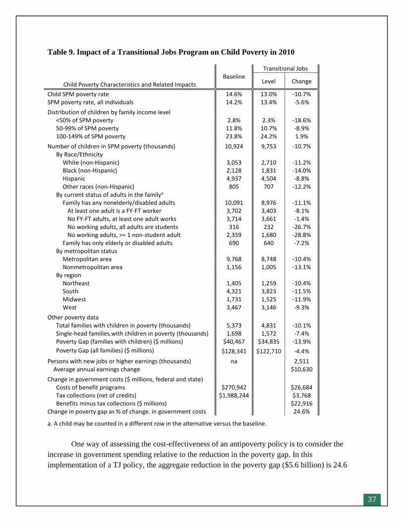
37
Table 9. Impact of a Transitional Jobs Program on Child Poverty in 2010
Child Poverty Characteristics and Related Impacts Baseline
Transitional Jobs
Level Change
Child SPM poverty rate 14.6% 13.0% -10.7% SPM poverty rate, all individuals 14.2% 13.4% -5.6%
Distribution of children by family income level
<50% of SPM poverty 2.8% 2.3% -18.6%
50-99% of SPM poverty 11.8% 10.7% -8.9%
100-149% of SPM poverty 23.8% 24.2% 1.9%
Number of children in SPM poverty (thousands) 10,924 9,753 -10.7%
By Race/Ethnicity
White (non-Hispanic) 3,053 2,710 -11.2%
Black (non-Hispanic) 2,128 1,831 -14.0%
Hispanic 4,937 4,504 -8.8%
Other races (non-Hispanic) 805 707 -12.2%
By current status of adults in the familya
Family has any nonelderly/disabled adults 10,091 8,976 -11.1%
At least one adult is a FY-FT worker 3,702 3,403 -8.1%
No FY-FT adults, at least one adult works 3,714 3,661 -1.4%
No working adults, all adults are students 316 232 -26.7%
No working adults, >= 1 non-student adult 2,359 1,680 -28.8%
Family has only elderly or disabled adults 690 640 -7.2%
By metropolitan status
Metropolitan area 9,768 8,748 -10.4%
Nonmetropolitan area 1,156 1,005 -13.1%
By region
Northeast 1,405 1,259 -10.4%
South 4,321 3,823 -11.5%
Midwest 1,731 1,525 -11.9%
West 3,467 3,146 -9.3%
Other poverty data
Total families with children in poverty (thousands) 5,373 4,831 -10.1%
Single-head families.with children in poverty (thousands) 1,698 1,572 -7.4%
Poverty Gap (families with children) ($ millions) $40,467 $34,835 -13.9%
Poverty Gap (all families) ($ millions) $128,341 $122,710 -4.4%
Persons with new jobs or higher earnings (thousands) na 2,511 Average annual earnings change $10,630
Change in government costs ($ millions, federal and state)
Costs of benefit programs $270,942 $26,684
Tax collections (net of credits) $1,988,244 $3,768
Benefits minus tax collections ($ millions) $22,916
Change in poverty gap as % of change. in government costs 24.6%
a. A child may be counted in a different row in the alternative versus the baseline.
One way of assessing the cost-effectiveness of an antipoverty policy is to consider the
increase in government spending relative to the reduction in the poverty gap. In this
implementation of a TJ policy, the aggregate reduction in the poverty gap ($5.6 billion) is 24.6
38
percent of the net increase in government spending ($22.9 billion). In other words, for each
dollar of new government spending, the poverty gap is reduced by just below 25 cents—and all
of that reduction is for families with children.35 The remaining money increases families’
incomes to levels above the SPM poverty threshold, or helps families whose incomes were
already above the poverty level before the simulation.
Child Support Pass-Through
The next component of the CDF policy package envisions a national-level pass-through and
disregard policy for child support income that is paid by the noncustodial parents of children
receiving TANF or SNAP. Under current law, families receiving TANF must surrender their
rights to child support to the state, so that the state collects all child support received by that
family to reimburse the state’s TANF expenses. However, some states allow a portion of child
support to be “passed through” to the family, so that the family receives both its TANF benefit
and some child support; such states usually also disregard some or all of the child support that is
passed through when determining the family’s income, so that the family’s TANF benefits are
not reduced due to having the child support income in-hand. In 2010, almost half of the states
transferred and disregarded some amount of child support income, but no state transferred and
disregarded all child support income (Kassabian et al. 2011). The policy proposed by CDF would
allow TANF families in all states to keep all child support that is paid on behalf of the children
in the family, and all child support income would be fully disregarded when calculating the
TANF benefit amount. The estimates show the effect of full pass-through of currently due child
support. Although a policy could be designed to pass through all collections of past-due child
support (child support arrears), modeling the effects of such a pass through was beyond the scope
of this study.36
The SNAP program does not include a disregard of any of the child support income
received by a family (although the amount of child support that a noncustodial parent pays is
deducted or disregarded from the income of that individual). The CDF proposal for SNAP would
also allow $100 in child support to be disregarded each month for each child on whose behalf
child support income is paid. The disregard would be used when calculating both SNAP
eligibility and benefit amounts. This is based in part on the federal policy regarding TANF, in
which the federal government waives its share of the first $100 of child support passed through
and disregarded for one child, and the first $200 for child support passed through and
disregarded for two or more children.
35 Note that throughout this report, we compute this statistic—the change in the poverty gap as a percentage of the
change in government spending—using the total change in the poverty gap. However, since the CDF policies are
focused on families with children, in almost all cases the change in the total poverty gap is essentially equivalent to
the change in the poverty gap for families with children. When that is not the case, it is noted in the discussion.
36 See Wheaton and Sorensen (2005) for estimates of the effect of distributing all child support arrears collected on
behalf of former welfare families through the Federal Tax Refund Offset Program to families.
39
Methods: To implement this policy proposal, we adjusted the parameters of the TANF
simulation to allow the full amount of child support paid by the noncustodial parent to be passed
through to the family, in all states. Also, all states were modeled to disregard all the passed-
through child support when calculating the family’s benefit. However, the state rules for
counting child support in the family’s income when initially determining TANF eligibility were
left in place. (Note that if all child support income was disregarded for TANF eligibility
purposes, families with high child support income amounts but very little other income could be
found eligible for TANF.) We also adjusted the parameters of the SNAP simulation,
incorporating the $100 disregard per child for both SNAP eligibility and the benefit amount.
The child support income amounts used to model the policy are a modified version of the
amounts reported in the CPS-ASEC survey. As mentioned earlier, child support income is
underreported by TANF families, since they may not directly receive most or any of their child
support income. TRIM3 procedures augment the child support income of TANF families to
account for this underreporting, with the adjustment calibrated using administrative data.
It is important to note that our simulation assumed that the payment of child support by
the noncustodial parents was unchanged from the baseline simulation. Some research has found
that child support pass-through/disregard policies can increase payments. For example, Lippold,
Nichols, and Sorensen (2010) found that noncustodial parents of children receiving TANF who
had a current child support order paid 5.6 percent more child support after a $150 pass-through
and disregard was instituted.
Results: When TANF includes a full child support pass-through and disregard for benefit
determination and SNAP includes a partial disregard of child support income, the child SPM
poverty rate decreases very slightly—from 14.6 percent in the baseline to 14.5 percent, a
decrease of 0.8 percent (table 10). The poverty gap for families with children falls by $270
million, or 0.7 percent. The relatively limited impact of the policy in aggregate terms is related to
the relatively small number of children who receive TANF; among the families with children
who are measured in this study as being in SPM poverty, fewer than one-fifth received TANF
income. Furthermore, not all TANF and SNAP families have child support income. Among
families with any TANF income during 2010, only 0.46 million had any child support income
paid on their behalf during months of TANF receipt (fewer than one in seven families with any
TANF in 2010), with child support payments during months of TANF receipt totaling $628
million in the simulation data (less than 2 percent of the $40.5 billion poverty gap for families
with children).
Implementing the full child support pass-through and disregard in the TANF program
substantially increases the amount of child support income distributed to TANF families, slightly
increases the TANF caseload, and slightly increases TANF benefits. Among families with TANF
in the baseline, the average monthly number with any pass-through increases from 179,000 to
40
250,000; an additional 19,000 families that were previously eligible are estimated to begin to
participate in TANF because of changes. Among families receiving TANF in the baseline, the
aggregate amount passed-through increases from $203 million in the baseline (of which $129
million is also disregarded for benefit computation) to $679 million (all of which is also
disregarded for benefit computation) (table C3.2a). The changes increase aggregate TANF
benefits by $97 million (1.2 percent), due in part to the new participants and in part to higher
benefits for some existing participants. In states that currently retain all child support, passing
through and disregarding all child support did not result in a change in benefits for any current
recipient; of course, the proposed policy would let those participants have the same TANF
benefit plus all the child support income. In states that currently pass through a portion of child
support but do not disregard all of it, the full disregard policy could result in a higher TANF
benefit.
In the much larger SNAP program, the proposed policy results in 1.12 million assistance
units being able to deduct a total of $2.6 billion in child support income (an average of $194 per
month, for families with child support income). Since the program previously counted all child
support income, the disregard increases SNAP benefits for many families, by as much as 30
percent of the disregarded child support income.37 However, for families with child support
receiving both TANF and SNAP, any increase in TANF works in the direction of decreasing
SNAP benefits. Aggregate SNAP benefits increase by $608 million, a 0.9 percent increase from
the baseline.
37 SNAP benefits are computed by starting from a maximum benefit and subtracting 30 percent of a family’s net
income—the portion they are assumed to be able to spend on food. Due to an interaction with the SNAP excess
shelter expense deduction, some households may experience benefit increases exceeding 30 percent of the
disregarded child support income.
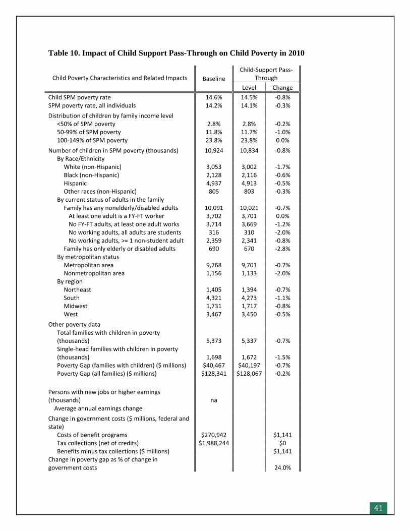
41
Table 10. Impact of Child Support Pass-Through on Child Poverty in 2010
Child Poverty Characteristics and Related Impacts Baseline
Child-Support Pass-Through
Level Change
Child SPM poverty rate 14.6% 14.5% -0.8% SPM poverty rate, all individuals 14.2% 14.1% -0.3%
Distribution of children by family income level <50% of SPM poverty 2.8% 2.8% -0.2% 50-99% of SPM poverty 11.8% 11.7% -1.0% 100-149% of SPM poverty 23.8% 23.8% 0.0%
Number of children in SPM poverty (thousands) 10,924 10,834 -0.8% By Race/Ethnicity White (non-Hispanic) 3,053 3,002 -1.7% Black (non-Hispanic) 2,128 2,116 -0.6% Hispanic 4,937 4,913 -0.5% Other races (non-Hispanic) 805 803 -0.3% By current status of adults in the family Family has any nonelderly/disabled adults 10,091 10,021 -0.7% At least one adult is a FY-FT worker 3,702 3,701 0.0% No FY-FT adults, at least one adult works 3,714 3,669 -1.2% No working adults, all adults are students 316 310 -2.0% No working adults, >= 1 non-student adult 2,359 2,341 -0.8% Family has only elderly or disabled adults 690 670 -2.8% By metropolitan status Metropolitan area 9,768 9,701 -0.7% Nonmetropolitan area 1,156 1,133 -2.0% By region Northeast 1,405 1,394 -0.7% South 4,321 4,273 -1.1% Midwest 1,731 1,717 -0.8% West 3,467 3,450 -0.5%
Other poverty data
Total families with children in poverty (thousands) 5,373 5,337 -0.7%
Single-head families with children in poverty (thousands) 1,698 1,672 -1.5%
Poverty Gap (families with children) ($ millions) $40,467 $40,197 -0.7% Poverty Gap (all families) ($ millions) $128,341 $128,067 -0.2%
Persons with new jobs or higher earnings (thousands) na
Average annual earnings change
Change in government costs ($ millions, federal and state) Costs of benefit programs $270,942 $1,141 Tax collections (net of credits) $1,988,244 $0 Benefits minus tax collections ($ millions) $1,141 Change in poverty gap as % of change in government costs 24.0%
42
Other programs also show secondary impacts from the TANF changes. Since housing
subsidy programs consider TANF as income when computing a subsidized household’s required
rental payment, the increased TANF income increases rental payments, decreasing the value of
housing subsidies by $41 million (0.1 percent). There was also a small ($0.5 million) reduction
in the value of child care subsidies, since some states count TANF as income in determining
CCDF eligibility and copayments.
Of course, a final key financial change for the government is that $477 million in child
support that was previously retained by the government to offset TANF costs is now transferred
to families. Combining that change with the changes in program spending, overall government
spending is estimated to increase by $1.1 billion. The aggregate change in the poverty gap is 24
percent of the $1.1 billion increase in government spending. In other words, for each dollar of
new government spending, the poverty gap is reduced by 24 cents—and all of that reduction is
for families with children. The remaining money increases families’ incomes to levels above the
SPM poverty threshold, or helps families whose incomes were already above the SPM poverty
level.
As mentioned earlier, the simulation did not model any change in the payments made by
noncustodial parents. To the extent that those parents increased the amount of child support that
they pay due to knowing that the custodial families would be able to keep it, government costs
might be lower than shown here (e.g., some families might become ineligible for certain
programs), and the antipoverty impacts might be somewhat higher.
Increasing In-Kind Income
A second avenue to reducing economic hardship for families with children is to increase a
family’s resources from in-kind benefits, such as assistance paying for food or housing. Since the
SPM counts these benefits in the resource measure, the antipoverty impacts of these sorts of
changes can be captured through the SPM and compared with the impacts of other types of
policy changes. The CDF package includes expansions to housing subsidies and an increase to
SNAP benefits.
Expanded Housing Assistance
This component of the CDF policy package provides additional housing vouchers to low-income
households with children with income under 150 percent of the poverty guideline that also
satisfy a test of rent burden. Although most Public Housing Authorities (PHAs) do not test for
rent burden, we include the test here to focus the benefits on households who could benefit the
most. There would be no change in the availability of vouchers for households without children.
A subsidized household’s required rental payment would be computed as in the existing Housing

43
Choice Voucher program, generally equal to 30 percent of net income. Also, as in the current
program, the new vouchers would be available only to citizens and legal immigrants.
The income limit for the proposed expansion—150 percent of the poverty guidelines—
differs from the current program’s income limits. Under current policies, to be initially eligible
for a housing voucher, a household’s income must be no more than half of the median income in
the PHA area where the household resides (area median income, or AMI); this is considered
“very low income” by the US Department of Housing and Urban Development (HUD).38 Median
incomes vary widely across the country. For example, for fiscal year 2010, 50 percent of AMI
for a family of four was $51,750 in Fairfax County, Virginia, $41,400 in Los Angeles County,
California, and $21,200 in Adams County, Mississippi.39 In contrast, 150 percent of the poverty
guideline for a family of four in 2010, in all of the contiguous states and Washington, D.C., was
$33,075.40 Thus, the income limit for the proposed expansion could be higher or lower than the
regular program’s income limit, depending on the area of the country.
A key difference between the proposed expansion and the current program is that the
proposed policy would not include waiting lists. Many households who are eligible for vouchers
(or public housing) are not able to obtain assistance due to waiting lists. Under the CDF
proposal, a housing voucher would be available to any household with children meeting all of the
eligibility criteria.
Methods: Simulating the housing program involved applying the initial program
eligibility requirements, estimating the required number of bedrooms, estimating the fair market
rent, imposing the rent burden test, and estimating what percentage of eligible households would
use the voucher. The new policy was imposed only to identify additional housing vouchers;
households in public or subsidized housing in the baseline simulation retain those subsidies.
Households with children were considered potentially eligible for a new voucher if they
were not already in public or subsidized housing, they reported in the survey that they rent their
home (i.e., do not own their home and do not live rent-free), the household included at least one
citizen, refugee/asylee, or legal permanent resident, and the household’s income was under 150
percent of the poverty guideline. In 2010, 150 percent of the poverty guideline was equivalent to
the following income limits for the contiguous states and Washington, DC:
38 For households already receiving vouchers, income may rise to 80 percent of area median income, considered
“low income.” See Chapter 5 of the “Housing Choice Voucher Program Guidebook,” on the HUD website,
http://portal.hud.gov/hudportal/HUD?src=/program_offices/public_indian_housing/programs/hcv/forms/guidebook.
39 See the FY 2010 Income Limits Documentation System on the HUD website,
http://www.huduser.org/portal/datasets/il/il2010/select_Geography.odn.
40 See the HHS/ASPE website, Poverty Guidelines page, http://aspe.hhs.gov/poverty/index.cfm.
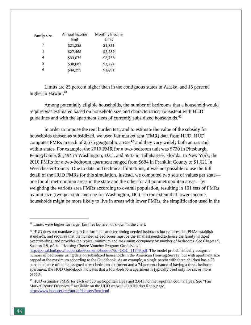
44
Family size Annual Income limit
Monthly Income Limit
2 $21,855 $1,821
3 $27,465 $2,289
4 $33,075 $2,756
5 $38,685 $3,224
6 $44,295 $3,691
Limits are 25 percent higher than in the contiguous states in Alaska, and 15 percent
higher in Hawaii.41
Among potentially eligible households, the number of bedrooms that a household would
require was estimated based on household size and characteristics, consistent with HUD
guidelines and with the apartment sizes of currently subsidized households.42
In order to impose the rent burden test, and to estimate the value of the subsidy for
households chosen as subsidized, we used fair market rent (FMR) data from HUD. HUD
computes FMRs in each of 2,575 geographic areas,43 and they vary widely both across and
within states. For example, the 2010 FMR for a two-bedroom unit was $730 in Pittsburgh,
Pennsylvania, $1,494 in Washington, D.C., and $943 in Tallahassee, Florida. In New York, the
2010 FMRs for a two-bedroom apartment ranged from $684 in Franklin County to $1,621 in
Westchester County. Due to data and technical limitations, it was not possible to use the full
detail of the HUD FMRs for this simulation. Instead, we computed two sets of values per state—
one for all metropolitan areas in the state and the other for all nonmetropolitan areas—by
weighting the various area FMRs according to overall population, resulting in 101 sets of FMRs
by unit size (two per state and one for Washington, DC). To the extent that lower-income
households might be more likely to live in areas with lower FMRs, the simplification used in the
41 Limits were higher for larger families but are not shown in the chart.
42 HUD does not mandate a specific formula for determining needed bedrooms but requires that PHAs establish
standards, and requires that the number of bedrooms must be the smallest needed to house the family without
overcrowding, and provides the typical minimum and maximum occupancy by number of bedrooms. See Chapter 5,
Section 5.9, of the “Housing Choice Voucher Program Guidebook”,
http://portal.hud.gov/hudportal/documents/huddoc?id=DOC_11749.pdf. The model probabilistically assigns a
number of bedrooms using data on subsidized households in the American Housing Survey, but with apartment size
capped at the maximum according to the Guidebook. As an example, a single parent with three children has a 26
percent chance of being assigned a two-bedroom apartment and a 74 percent chance of having a three-bedroom
apartment; the HUD Guidebook indicates that a four-bedroom apartment is typically used only for six or more
people.
43 HUD estimates FMRs for each of 530 metropolitan areas and 2,045 nonmetropolitan county areas. See “Fair
Market Rents: Overview,” available on the HUD website, Fair Market Rents page,
http://www.huduser.org/portal/datasets/fmr.html.
45
simulation could result in assigning values somewhat higher than what the actual FMRs would
be.
Among the potentially eligible households, the simulation uses the 101 sets of average
FMR figures to estimate rent burden. A low-income household was considered to need a voucher
only if the applicable FMR for the size of apartment needed by the household was higher than 50
percent of the household’s gross cash income. For example, since the average two-bedroom
FMR for urban areas in Virginia in 2010 was $1,076, an urban Virginia household needing a
two-bedroom apartment was considered to need a subsidy if gross monthly income was less than
two times that figure, or less than $2,152. This aspect of the eligibility test is based in part on
analysis by HUD (2013), which considers a household with rent equal to more than half of its
income to have “worst case housing needs.”
Among households passing all the eligibility criteria, including the rent burden test, the
model selects 70 percent to successfully use a voucher. The assumption is that all eligible
households would want a housing voucher, but that 30 percent of those households would not be
able to find an apartment and use the voucher. The assumption of 70 percent is based on a 2001
HUD study of success rates in the Housing Choice Voucher Program (Finkel and Buron 2001).
The research found a range of success rates across public housing agencies, from 37 percent to
100 percent, but the most common outcome was that 61 to 70 percent of households successfully
used vouchers. Nationally, the study estimated that 69 percent of households receiving vouchers
from large metropolitan PHAs succeeded in using them to lease units. In the simulation, the
specific households chosen as successfully using the new vouchers are selected randomly from
among those satisfying all the eligibility criteria.
For each household simulated to receive and use a new voucher, we computed the
required rental payment, following the rules of the current Housing Choice Voucher program
regarding deductions from income and rent computation. We also computed the value of the
subsidy, all or part of which is considered an element of resources in the SPM poverty
computation. (The amount of housing subsidy included as an SPM resource is capped at 49.7
percent of the level of the SPM threshold, minus the family’s required rental contribution.) The
subsidy is computed as the assumed FMR minus the household’s required rental payment. This
implicitly assumes that PHAs compute payments to owners using the FMRs, and that each
subsidized household finds an apartment with a total rent exactly equal to the FMR. Thus, the
simulation does not capture the real-world nuances that some households might find apartments
with rents lower than the FMR, and that PHAs are allowed to set their “payment standards” (for
payments to apartment owners) between 90 percent and 110 percent of the published FMRs.44
44 See Section 7.1 of the “Housing Choice Voucher Program Guidebook,” on the HUD website,
http://portal.hud.gov/hudportal/HUD?src=/program_offices/public_indian_housing/programs/hcv/forms/guidebook.
46
The fact that many households pay lower rents after receiving the voucher has a
secondary impact on SNAP benefits. The computation of SNAP benefits involves a deduction
from income that is based on a household’s shelter expenses; lower shelter expenses result in
higher net incomes for some families, which result in lower SNAP benefits. For some families, a
lower shelter deduction could make them ineligible for SNAP benefits.
The simulation does not model any behavioral impacts that could result from housing
vouchers. Vouchers could improve long-run employment outcomes by improving family
stability, but could also reduce the incentive to work due to increasing family resources and due
to the fact that the voucher program includes an implicit “tax” on earnings (since the family’s
required rental payment is higher when earnings are higher). A 2006 study for HUD focusing on
families receiving welfare (Mills et. al. 2006) found that using a voucher reduced employment
rates and earnings amounts in the first year or two after random assignment, but the impact was
small and vouchers had no significant impact after several years.
Results: The specifications above resulted in 2.6 million households with children newly
receiving housing subsidies—a 53 percent increase from the 4.9 million households who are in
public or subsidized housing in the baseline (table C3.3a). On average, the annual value of the
subsidy for newly subsidized households is $9,435, or about $786 per month.
The housing voucher policy was one of the more successful individual programs in the
CDF package in terms of reducing child poverty. Compared to the baseline, the housing program
reduced child poverty by 20.8 percent, from a rate of 14.6 percent to a rate of 11.5 percent (table
11). The poverty gap for families with children fell by $11.5 billion or 28.5 percent from the
baseline level. (The poverty gap for all families falls by $11.6 billion; the slight difference is due
to the fact that a small number of newly assisted households have more than one family for
poverty calculation purposes.)
Children in the lowest income levels saw the greatest impact, as these families are more
likely to face rents that exceed 50 percent of their gross income. The greatest reductions were
also seen in metropolitan areas as well as the Northeast and West, places where families likely
face higher rents. With equivalent income, households were more likely to pass the rent-burden
test in high-rent versus low-rent areas. The percentage reduction in child poverty is smaller for
white children (a 14.7 percent reduction) than for nonwhite children (a reduction of 23.2 percent
combining all the nonwhite categories), which may be due in part to variations in the geographic
locations of white children in poverty versus nonwhite children in poverty.
The net cost of the program (excluding administrative costs) is estimated at $23.5 billion
during 2010. The aggregate annual value of the subsidies increases by $24.4 billion, a 70 percent
increase from the baseline. This cost is slightly offset by a reduction of $0.9 billion in
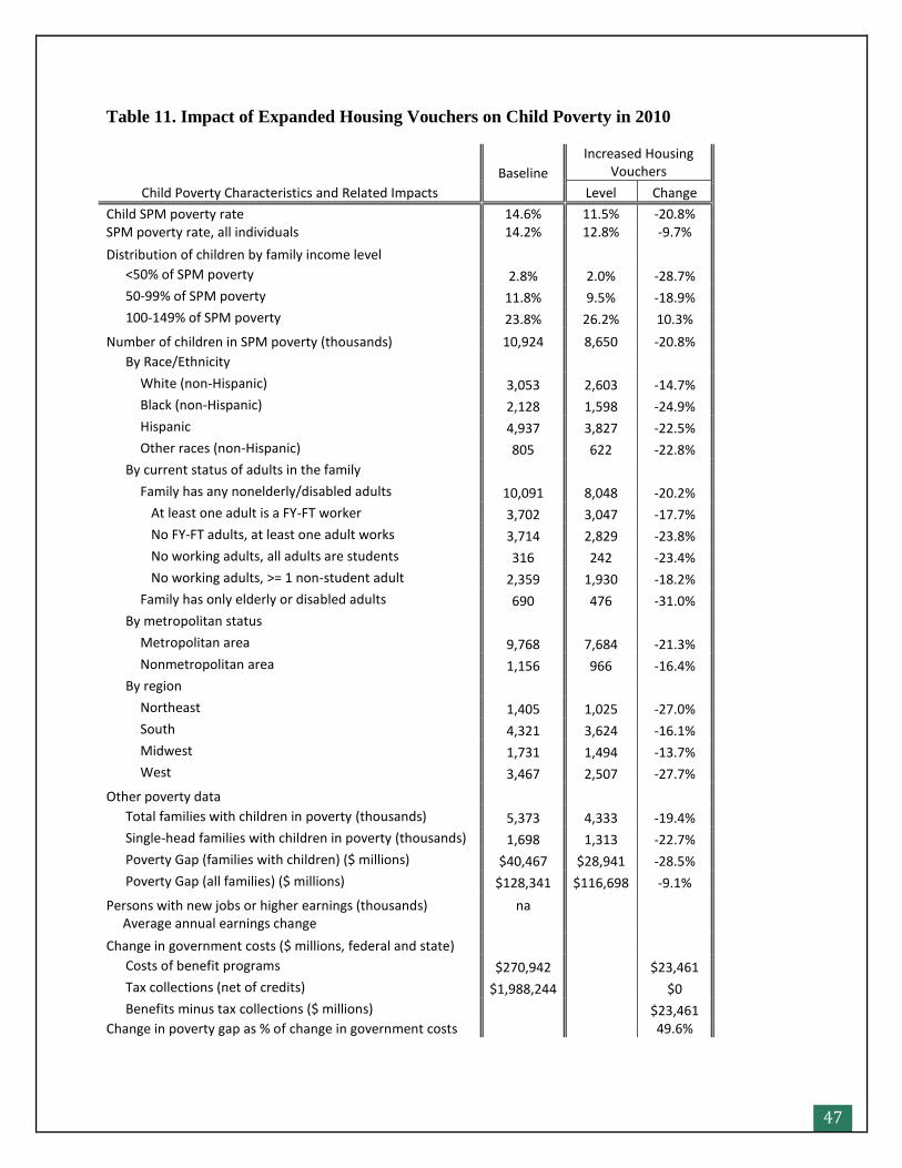
47
Table 11. Impact of Expanded Housing Vouchers on Child Poverty in 2010
Child Poverty Characteristics and Related Impacts
Baseline
Increased Housing Vouchers
Level Change
Child SPM poverty rate 14.6% 11.5% -20.8% SPM poverty rate, all individuals 14.2% 12.8% -9.7%
Distribution of children by family income level
<50% of SPM poverty 2.8% 2.0% -28.7%
50-99% of SPM poverty 11.8% 9.5% -18.9%
100-149% of SPM poverty 23.8% 26.2% 10.3%
Number of children in SPM poverty (thousands) 10,924 8,650 -20.8%
By Race/Ethnicity
White (non-Hispanic) 3,053 2,603 -14.7%
Black (non-Hispanic) 2,128 1,598 -24.9%
Hispanic 4,937 3,827 -22.5%
Other races (non-Hispanic) 805 622 -22.8%
By current status of adults in the family
Family has any nonelderly/disabled adults 10,091 8,048 -20.2%
At least one adult is a FY-FT worker 3,702 3,047 -17.7%
No FY-FT adults, at least one adult works 3,714 2,829 -23.8%
No working adults, all adults are students 316 242 -23.4%
No working adults, >= 1 non-student adult 2,359 1,930 -18.2%
Family has only elderly or disabled adults 690 476 -31.0%
By metropolitan status
Metropolitan area 9,768 7,684 -21.3%
Nonmetropolitan area 1,156 966 -16.4%
By region
Northeast 1,405 1,025 -27.0%
South 4,321 3,624 -16.1%
Midwest 1,731 1,494 -13.7%
West 3,467 2,507 -27.7%
Other poverty data
Total families with children in poverty (thousands) 5,373 4,333 -19.4%
Single-head families with children in poverty (thousands) 1,698 1,313 -22.7%
Poverty Gap (families with children) ($ millions) $40,467 $28,941 -28.5%
Poverty Gap (all families) ($ millions) $128,341 $116,698 -9.1%
Persons with new jobs or higher earnings (thousands) na Average annual earnings change
Change in government costs ($ millions, federal and state)
Costs of benefit programs $270,942 $23,461
Tax collections (net of credits) $1,988,244 $0
Benefits minus tax collections ($ millions) $23,461 Change in poverty gap as % of change in government costs 49.6%
48
SNAP benefits, due to the interaction between rent payments and the SNAP program’s shelter
deduction. The change in the poverty gap as a percentage of the change in government costs is
49.6 percent. In other words, for each dollar of new government spending, the poverty gap is
reduced by almost 50 cents; and almost all of that poverty gap reduction is for families with
children. The remaining money increases families’ incomes to levels above the SPM poverty
threshold, or helps families whose incomes were already above the poverty level before the
simulation.
SNAP Benefit Increase
Another component of the CDF policy package increases the SNAP maximum benefits for
SNAP assistance units with children. (The proposal leaves SNAP benefits for households
without children unchanged.45) SNAP benefits are computed by starting from a set of maximum
benefits (which vary by household size) and then subtracting 30 percent of a household’s net
income—since the household is assumed to be able to spend that portion of their income on
food. The maximum benefits currently used by the program are a set of values known as the
Thrifty Food Plan. However, the US Department of Agriculture (USDA) also computes other
food plan values. Under this proposal, SNAP benefits for households with children would be
calculated using the Low-Cost Food Plan—a set of values that is 30 percent higher on average
from Thrifty Food Plan values (Hartline-Grafton and Weill 2012), and the second-lowest tier of
food costs computed by USDA. The maximum increase in the annual benefit for a three-person
family would be $1,896.
Methods: Simulating the higher SNAP benefit amounts required computing a specific set
of hypothetical benefit amounts and determining the impact on program participation.
The computation of the hypothetical benefits was complicated by two factors. The first
complication is the fact that SNAP benefits were increased by 13.6 percent by the American
Recovery and Reinvestment Act of 2009 (ARRA). This temporary increase was still in place in
2010 and was included in the baseline simulation (see Appendix B for more information on the
ARRA provisions and the impact of removing the provisions). Thus, the baseline already
includes an increase relative to the standard SNAP benefit levels.
The second complication is the fact that SNAP benefits are computed based on family
size, regardless of family composition, but USDA provides food plan amounts only at the
individual level (e.g., for females ages 14 to 18, males ages 71 or older), and for four
prototypical family compositions (e.g., the Low-Cost Food Plan required that a couple with two
45 For comparison, Appendix C includes the cost and poverty impacts of applying the policy change described here
for all SNAP households, not just those with children.
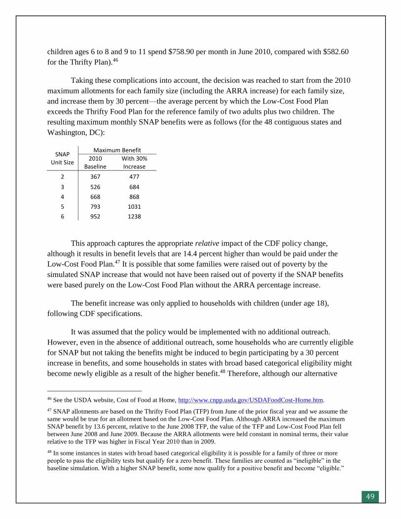
49
children ages 6 to 8 and 9 to 11 spend $758.90 per month in June 2010, compared with $582.60
for the Thrifty Plan).46
Taking these complications into account, the decision was reached to start from the 2010
maximum allotments for each family size (including the ARRA increase) for each family size,
and increase them by 30 percent—the average percent by which the Low-Cost Food Plan
exceeds the Thrifty Food Plan for the reference family of two adults plus two children. The
resulting maximum monthly SNAP benefits were as follows (for the 48 contiguous states and
Washington, DC):
SNAP Unit Size
Maximum Benefit
2010 Baseline
With 30% Increase
2 367 477
3 526 684
4 668 868
5 793 1031
6 952 1238
This approach captures the appropriate relative impact of the CDF policy change,
although it results in benefit levels that are 14.4 percent higher than would be paid under the
Low-Cost Food Plan.47 It is possible that some families were raised out of poverty by the
simulated SNAP increase that would not have been raised out of poverty if the SNAP benefits
were based purely on the Low-Cost Food Plan without the ARRA percentage increase.
The benefit increase was only applied to households with children (under age 18),
following CDF specifications.
It was assumed that the policy would be implemented with no additional outreach.
However, even in the absence of additional outreach, some households who are currently eligible
for SNAP but not taking the benefits might be induced to begin participating by a 30 percent
increase in benefits, and some households in states with broad based categorical eligibility might
become newly eligible as a result of the higher benefit.48 Therefore, although our alternative
46 See the USDA website, Cost of Food at Home, http://www.cnpp.usda.gov/USDAFoodCost-Home.htm.
47 SNAP allotments are based on the Thrifty Food Plan (TFP) from June of the prior fiscal year and we assume the
same would be true for an allotment based on the Low-Cost Food Plan. Although ARRA increased the maximum
SNAP benefit by 13.6 percent, relative to the June 2008 TFP, the value of the TFP and Low-Cost Food Plan fell
between June 2008 and June 2009. Because the ARRA allotments were held constant in nominal terms, their value
relative to the TFP was higher in Fiscal Year 2010 than in 2009.
48 In some instances in states with broad based categorical eligibility it is possible for a family of three or more
people to pass the eligibility tests but qualify for a zero benefit. These families are counted as “ineligible” in the
baseline simulation. With a higher SNAP benefit, some now qualify for a positive benefit and become “eligible.”
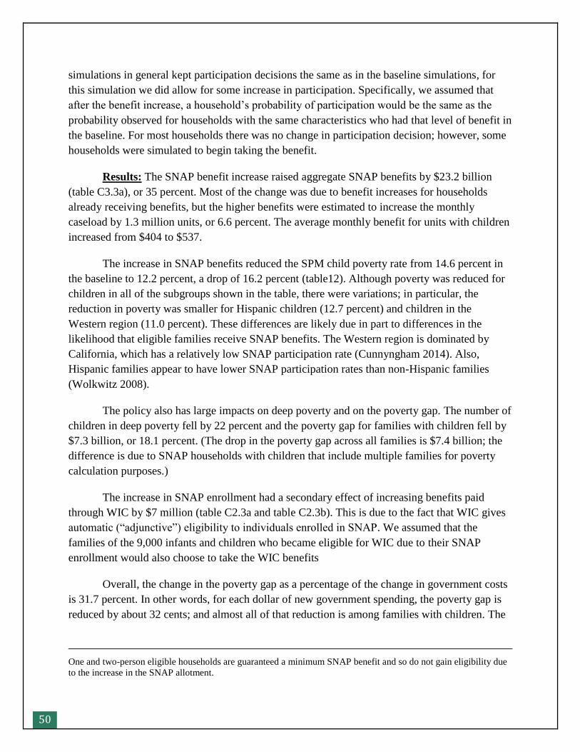
50
simulations in general kept participation decisions the same as in the baseline simulations, for
this simulation we did allow for some increase in participation. Specifically, we assumed that
after the benefit increase, a household’s probability of participation would be the same as the
probability observed for households with the same characteristics who had that level of benefit in
the baseline. For most households there was no change in participation decision; however, some
households were simulated to begin taking the benefit.
Results: The SNAP benefit increase raised aggregate SNAP benefits by $23.2 billion
(table C3.3a), or 35 percent. Most of the change was due to benefit increases for households
already receiving benefits, but the higher benefits were estimated to increase the monthly
caseload by 1.3 million units, or 6.6 percent. The average monthly benefit for units with children
increased from $404 to $537.
The increase in SNAP benefits reduced the SPM child poverty rate from 14.6 percent in
the baseline to 12.2 percent, a drop of 16.2 percent (table12). Although poverty was reduced for
children in all of the subgroups shown in the table, there were variations; in particular, the
reduction in poverty was smaller for Hispanic children (12.7 percent) and children in the
Western region (11.0 percent). These differences are likely due in part to differences in the
likelihood that eligible families receive SNAP benefits. The Western region is dominated by
California, which has a relatively low SNAP participation rate (Cunnyngham 2014). Also,
Hispanic families appear to have lower SNAP participation rates than non-Hispanic families
(Wolkwitz 2008).
The policy also has large impacts on deep poverty and on the poverty gap. The number of
children in deep poverty fell by 22 percent and the poverty gap for families with children fell by
$7.3 billion, or 18.1 percent. (The drop in the poverty gap across all families is $7.4 billion; the
difference is due to SNAP households with children that include multiple families for poverty
calculation purposes.)
The increase in SNAP enrollment had a secondary effect of increasing benefits paid
through WIC by $7 million (table C2.3a and table C2.3b). This is due to the fact that WIC gives
automatic (“adjunctive”) eligibility to individuals enrolled in SNAP. We assumed that the
families of the 9,000 infants and children who became eligible for WIC due to their SNAP
enrollment would also choose to take the WIC benefits
Overall, the change in the poverty gap as a percentage of the change in government costs
is 31.7 percent. In other words, for each dollar of new government spending, the poverty gap is
reduced by about 32 cents; and almost all of that reduction is among families with children. The
One and two-person eligible households are guaranteed a minimum SNAP benefit and so do not gain eligibility due
to the increase in the SNAP allotment.

51
remaining money increases families’ incomes to levels above the SPM poverty threshold, or
helps families whose incomes were already above the poverty level before the simulation.
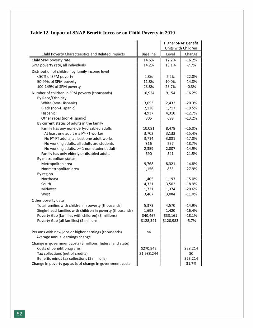
52
Table 12. Impact of SNAP Benefit Increase on Child Poverty in 2010
Child Poverty Characteristics and Related Impacts Baseline
Higher SNAP Benefit Units with Children
Level Change
Child SPM poverty rate 14.6% 12.2% -16.2% SPM poverty rate, all individuals 14.2% 13.1% -7.7%
Distribution of children by family income level <50% of SPM poverty 2.8% 2.2% -22.0% 50-99% of SPM poverty 11.8% 10.0% -14.8% 100-149% of SPM poverty 23.8% 23.7% -0.3%
Number of children in SPM poverty (thousands) 10,924 9,154 -16.2% By Race/Ethnicity White (non-Hispanic) 3,053 2,432 -20.3% Black (non-Hispanic) 2,128 1,713 -19.5% Hispanic 4,937 4,310 -12.7% Other races (non-Hispanic) 805 699 -13.2% By current status of adults in the family Family has any nonelderly/disabled adults 10,091 8,478 -16.0% At least one adult is a FY-FT worker 3,702 3,133 -15.4% No FY-FT adults, at least one adult works 3,714 3,081 -17.0% No working adults, all adults are students 316 257 -18.7% No working adults, >= 1 non-student adult 2,359 2,007 -14.9% Family has only elderly or disabled adults 690 541 -21.5% By metropolitan status Metropolitan area 9,768 8,321 -14.8% Nonmetropolitan area 1,156 833 -27.9% By region Northeast 1,405 1,193 -15.0% South 4,321 3,502 -18.9% Midwest 1,731 1,374 -20.6% West 3,467 3,084 -11.0%
Other poverty data Total families with children in poverty (thousands) 5,373 4,570 -14.9% Single-head families with children in poverty (thousands) 1,698 1,420 -16.4% Poverty Gap (families with children) ($ millions) $40,467 $33,161 -18.1% Poverty Gap (all families) ($ millions) $128,341 $120,983 -5.7%
Persons with new jobs or higher earnings (thousands) na Average annual earnings change
Change in government costs ($ millions, federal and state) Costs of benefit programs $270,942 $23,214 Tax collections (net of credits) $1,988,244 $0 Benefits minus tax collections ($ millions) $23,214 Change in poverty gap as % of change in government costs 31.7%
53
Reducing Taxes
Since tax liabilities are subtracted from SPM resources, and tax credits are added to resources,
changes to the tax code can have considerable impacts on SPM poverty. The CDF package
includes three types of tax credit expansions: an expanded Earned Income Tax Credit, a fully
refundable Child Tax Credit, and an expanded Child and Dependent Care Tax Credit.
Expanded Earned Income Tax Credit
This policy would expand the current Earned Income Tax Credit (EITC) for adults with children,
providing a larger credit at lower levels of income while phasing out at the same rate.
Specifically, the revised credit would phase in at a greater rate but reach the “plateau” region
(where the credit does not increase with earned income) at an earlier point, and begin decreasing
the credit at a lower level of income (but at the same marginal tax rate), as indicated in Table 13.
Table 13. Parameters for EITC Proposal
2010 Baseline Values
Filing Status Children
Phase-In Rate
Plateau Begins
Max Credit
Plateau Ends
Phase-Out Rate
Single 0 7.65% $5,980 $457 $7,480 7.65%
1 34.00% $8,970 $3,050 $16,450 15.98%
2 40.00% $12,590 $5,036 $16,450 21.06%
3+ 45.00% $12,590 $5,666 $16,450 21.06%
Joint 0 7.65% $5,980 $457 $12,490 7.65%
1 34.00% $8,970 $3,050 $21,460 15.98%
2 40.00% $12,590 $5,036 $21,460 21.06%
3+ 45.00% $12,590 $5,666 $21,460 21.06%
CDF Proposal
Filing Status Children
Phase-In Rate
Plateau Begins
Max Credit
Plateau Ends
Phase-Out Rate
Single 0 7.65% $5,980 $457 $7,480 7.65%
1 68.00% $5,965 $4,056 $10,155 15.98%
2 74.00% $8,165 $6,042 $11,673 21.06%
3+ 79.00% $9,476 $7,486 $13,336 25.00%
Joint 0 7.65% $5,980 $457 $12,490 7.65%
1 68.00% $5,965 $4,056 $15,162 15.98%
2 74.00% $8,165 $6,042 $16,683 21.06%
3+ 79.00% $9,476 $7,486 $18,346 24.94%
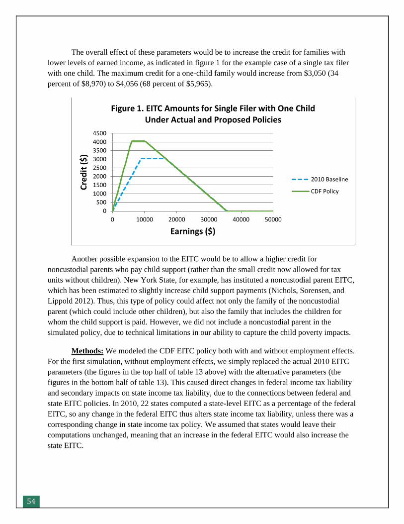
54
The overall effect of these parameters would be to increase the credit for families with
lower levels of earned income, as indicated in figure 1 for the example case of a single tax filer
with one child. The maximum credit for a one-child family would increase from $3,050 (34
percent of $8,970) to $4,056 (68 percent of $5,965).
Another possible expansion to the EITC would be to allow a higher credit for
noncustodial parents who pay child support (rather than the small credit now allowed for tax
units without children). New York State, for example, has instituted a noncustodial parent EITC,
which has been estimated to slightly increase child support payments (Nichols, Sorensen, and
Lippold 2012). Thus, this type of policy could affect not only the family of the noncustodial
parent (which could include other children), but also the family that includes the children for
whom the child support is paid. However, we did not include a noncustodial parent in the
simulated policy, due to technical limitations in our ability to capture the child poverty impacts.
Methods: We modeled the CDF EITC policy both with and without employment effects.
For the first simulation, without employment effects, we simply replaced the actual 2010 EITC
parameters (the figures in the top half of table 13 above) with the alternative parameters (the
figures in the bottom half of table 13). This caused direct changes in federal income tax liability
and secondary impacts on state income tax liability, due to the connections between federal and
state EITC policies. In 2010, 22 states computed a state-level EITC as a percentage of the federal
EITC, so any change in the federal EITC thus alters state income tax liability, unless there was a
corresponding change in state income tax policy. We assumed that states would leave their
computations unchanged, meaning that an increase in the federal EITC would also increase the
state EITC.
0
500
1000
1500
2000
2500
3000
3500
4000
4500
0 10000 20000 30000 40000 50000
Cre
dit
($
)
Earnings ($)
Figure 1. EITC Amounts for Single Filer with One Child Under Actual and Proposed Policies
2010 Baseline
CDF Policy

55
The second simulation of the EITC policy adds a behavioral impact: an increase in the
number of single parents who are working. The EITC increases an individual’s effective wage,
and there is general consensus that EITC increases can increase labor supply (see, for example,
Eissa and Hoynes 2006). Our methodology for this effect was similar to our methods used in
prior TRIM3 analyses (Giannarelli, Lippold, and Martinez-Schiferl 2012). Specifically, we
assumed that a roughly $1,000 increase in the maximum credit (as proposed) would encourage
enough single family heads to begin to work to lead to a 3.6 percentage point increase in the
employment to population ratio for single family heads, following the empirical results from
Grogger (2003). (Eissa and Hoynes point out that there is a relatively narrow range in the
estimates of the impact of the EITC on the labor supply of single taxpayers.) We assumed no
effect on employment for married couples, given that the effects of the EITC on employment for
this group are ambiguous in the literature. As mentioned earlier, there is substantial uncertainty
in estimating these types of effects, in part because the assumptions are based on the impacts of
prior policy changes at prior points in time.
To select which additional single family heads would begin to work, we identified
individuals who were not working, unmarried, were heads of a family including children under
18, were eligible for the expanded EITC after taking a job, and were not disabled, students, or
over age 69 (as we considered these people unlikely to begin to work). We then randomly
selected enough of these individuals to take jobs to result in a 3.6 percentage point increase in the
proportion of single-family heads who were employed. This process raised the portion of adults
in single-parent families that were working from 59.7 percent in the baseline to 63.3 percent in
the simulation of the EITC with employment effects. Individuals simulated to take new jobs
were assigned full-year jobs at the minimum wage, with hours worked based on the
characteristics of jobs held by workers in SPM poverty in the 2010 baseline (specifically, we
assumed that 47 percent of new workers would work for 40 hours per week, 19 percent for 30
hours, 18 percent for 20 hours, 8 percent for 10 hours, and 9 percent for 50 hours).
Single parents with new jobs and with younger children would likely need to arrange for
child care. For parents who became eligible for CCDF child care subsidies, we assumed the same
probability of enrolling in CCDF as for families with similar characteristics in the baseline
simulation.49
As noted earlier, the baseline simulation identifies only 20.2 million tax units apparently
eligible for the EITC, falling 26 percent short of the total 27.4 million units who benefitted from
the EITC on their 2010 tax return. In dollar terms, the model simulates $37.2 billion in EITC in
49 The CCDF participation probabilities are based on a comparison of TRIM-simulated CCDF-eligible families with
families actually receiving CCDF-funded child care subsidies according to administrative data. Among eligible
families, the probability of receiving CCDF subsidies varies by race/ethnicity (highest for non-Hispanic black
families, lowest for Hispanics), ages of children (higher for children ages 1 through 5 than for infants or school-age
children), and income level (higher for lower-income families versus. families closer to the income limits).
56
2010 compared to the total $59.6 billion paid that year. A large share of the shortfall is
attributable to the fact that TRIM3 does not model noncompliance with EITC rules. The US
Department of Treasury estimates that between $15.3 billion and $18.4 billion in EITC payments
were issued improperly in 2010 (TIGTA 2014), representing a large share of the $22.3 billion
TRIM3 shortfall. Other possible explanations for the underidentification are that the model does
not allocate children within complex households so as to maximize tax benefits and does not
capture the fact that some survey-reported earnings are non-taxable (thereby lowering earnings
sufficiently for a tax unit to be eligible for the EITC). The procedures for modeling the EITC
were not changed for this simulation—only the parameters of the calculation.
Results: With no employment effects, expanding the EITC in the manner proposed by
CDF increased the total amount of credit by $7.5 billion, or 20.2 percent (table C2.4a). There
was no change in the number of units with the credit, due to the design of the expansion; as noted
above, the model’s underidentification of units with the EITC means that the dollar increase is
also likely underestimated. The average value of the federal EITC for a one-child family
increased from $1,865 in the baseline to $2,244 with the expanded credit. For a family with two
or more children, the average credit increased from $3,088 to $3,751.
State income tax liability fell by a total of $314 million across the states that compute a
state EITC as a percentage of the federal EITC. The majority of the reduction was in New York
State, with a state EITC equal to 30 percent of the federal credit in 2010; New York State tax
liability fell by $117 million or 0.5 percent. Combining the federal and state income tax results,
there was a total reduction in government tax collections of $7.8 billion. The reduced taxes
increased families’ resources, reducing the SPM child poverty rate from 14.6 percent to 13.9
percent, a 4.7 percent reduction (table 14).
When employment effects were modeled, 463,000 individuals were identified as starting
to work due to the increase in the effective wage caused by the EITC. As explained above, the
new workers were unmarried parents who became eligible for the EITC by starting to work. The
new workers thus all begin to take the EITC, increasing the total number of federal tax units with
the credit by 2.3 percent. Including the tax units of the new workers, the average credits are
$2,278 for families with one child and $3,814 for families with two or more children. The
aggregate increase in the federal EITC is estimated at $9.7 billion, and there are also increases in
state EITC and in the federal child tax credit and child and dependent care tax credit. However,
payroll taxes increase as a result of the new earnings. Combining the impacts on payroll taxes,
federal income taxes, and state income taxes, tax liability falls by $9.5 billion when the expanded
EITC is modeled with employment effects.
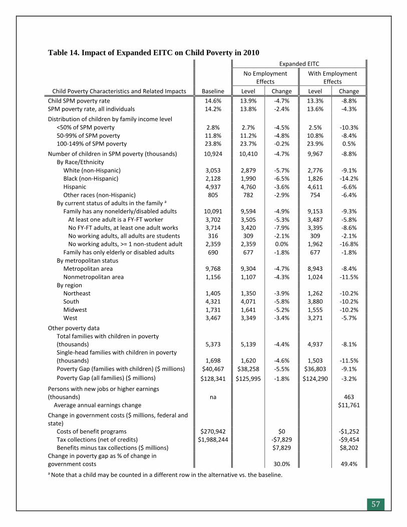
57
Table 14. Impact of Expanded EITC on Child Poverty in 2010
Child Poverty Characteristics and Related Impacts Baseline
Expanded EITC
No Employment Effects
With Employment Effects
Level Change Level Change
Child SPM poverty rate 14.6% 13.9% -4.7% 13.3% -8.8% SPM poverty rate, all individuals 14.2% 13.8% -2.4% 13.6% -4.3%
Distribution of children by family income level
<50% of SPM poverty 2.8% 2.7% -4.5% 2.5% -10.3%
50-99% of SPM poverty 11.8% 11.2% -4.8% 10.8% -8.4%
100-149% of SPM poverty 23.8% 23.7% -0.2% 23.9% 0.5%
Number of children in SPM poverty (thousands) 10,924 10,410 -4.7% 9,967 -8.8%
By Race/Ethnicity
White (non-Hispanic) 3,053 2,879 -5.7% 2,776 -9.1%
Black (non-Hispanic) 2,128 1,990 -6.5% 1,826 -14.2%
Hispanic 4,937 4,760 -3.6% 4,611 -6.6%
Other races (non-Hispanic) 805 782 -2.9% 754 -6.4%
By current status of adults in the family a
Family has any nonelderly/disabled adults 10,091 9,594 -4.9% 9,153 -9.3%
At least one adult is a FY-FT worker 3,702 3,505 -5.3% 3,487 -5.8%
No FY-FT adults, at least one adult works 3,714 3,420 -7.9% 3,395 -8.6%
No working adults, all adults are students 316 309 -2.1% 309 -2.1%
No working adults, >= 1 non-student adult 2,359 2,359 0.0% 1,962 -16.8%
Family has only elderly or disabled adults 690 677 -1.8% 677 -1.8%
By metropolitan status
Metropolitan area 9,768 9,304 -4.7% 8,943 -8.4%
Nonmetropolitan area 1,156 1,107 -4.3% 1,024 -11.5%
By region
Northeast 1,405 1,350 -3.9% 1,262 -10.2%
South 4,321 4,071 -5.8% 3,880 -10.2%
Midwest 1,731 1,641 -5.2% 1,555 -10.2%
West 3,467 3,349 -3.4% 3,271 -5.7%
Other poverty data
Total families with children in poverty (thousands) 5,373 5,139 -4.4% 4,937 -8.1%
Single-head families with children in poverty (thousands) 1,698 1,620 -4.6% 1,503 -11.5%
Poverty Gap (families with children) ($ millions) $40,467 $38,258 -5.5% $36,803 -9.1%
Poverty Gap (all families) ($ millions) $128,341 $125,995 -1.8% $124,290 -3.2%
Persons with new jobs or higher earnings (thousands) na
463 Average annual earnings change
$11,761
Change in government costs ($ millions, federal and state)
Costs of benefit programs $270,942 $0 -$1,252
Tax collections (net of credits) $1,988,244 -$7,829 -$9,454
Benefits minus tax collections ($ millions) $7,829 $8,202
Change in poverty gap as % of change in government costs 30.0% 49.4%
a Note that a child may be counted in a different row in the alternative vs. the baseline.
58
The new earnings modeled in the employment-effects scenario result in some decreases
in government benefits, the largest of which is an $894 million reduction in SNAP benefits.
However, the costs of child care subsidies increases, as 73,000 of the new workers are estimated
to begin taking CCDF-funded child care subsidies. On net, the cost of government benefits
decreases by $1.3 billion in this scenario, offsetting a portion of the reduction in tax liability to
produce an overall $8.2 billion increase in government costs.
Combining all the impacts—additional earnings, higher tax credits, lower benefits—the
EITC policy with employment effects reduces the child poverty rate to 13.3 percent, an 8.8
percent drop from the baseline. The largest decrease in poverty was for black children, with a
14.2 percent reduction assuming more single-family heads begin to work. The percentage
reduction in poverty was greater in families where adults work part-time or part-year (8.6
percent) compared with families with a full-year full-time worker (5.8 percent), as part-year or
part-time workers tend to have lower earned incomes and so are most likely to be in the range of
incomes affected by the EITC expansion. The number of children in poverty who live with
nondisabled working-age adults who are neither working or in school falls by 16.8 percent due to
the new employment; these children are then classified as living with working adults, although
they may still be poor.
The poverty gap for families with children fell by $3.7 billion, or 9.1 percent, when
employment effects are included. Overall, the poverty gap fell by $4.1 billion, or 3.2 percent.
The difference is due to the fact that some families with children older than 17 benefit from the
EITC. The change in the overall poverty gap as a percentage of the change in government costs
is 30.0 percent with no employment effects and 49.4 percent in the scenario with employment
effects. In other words, for each dollar of new government spending, the poverty gap is reduced
by about 30 cents without considering employment effects and by 49 cents if there is new
employment. (Since the new employment is assumed to be from private jobs, it increases family
incomes without increasing government costs.) The remaining money increases families’
incomes to levels above the SPM poverty threshold, or helps families whose incomes were
already above the poverty level before the simulation.
Because of the underidentification of actual EITC discussed above, the estimates likely
understate both the number of families that would benefit from the expansion and the aggregate
increase in the credit. The effect on EITC costs would depend largely on how often the
unidentified EITC recipients are in households with children in the portion of the EITC income
range affected by the EITC expansion. The effect of the shortfall on child poverty also depends
on how often the dollars not identified in the simulation would go to taxpayers without
qualifying children. The IRS estimates that over half of the total amount of EITC overclaims is
paid to taxpayers without qualifying children (IRS 2014), although some of those recipients
could live with children or use the credit to benefit children living elsewhere. Thus, the
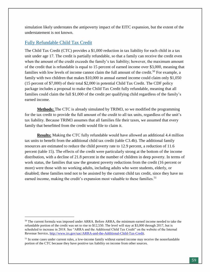
59
simulation likely understates the antipoverty impact of the EITC expansion, but the extent of the
understatement is not known.
Fully Refundable Child Tax Credit
The Child Tax Credit (CTC) provides a $1,000 reduction in tax liability for each child in a tax
unit under age 17. The credit is partially refundable, so that a family can receive the credit even
when the amount of the credit exceeds the family’s tax liability; however, the maximum amount
of the credit that is refundable is equal to 15 percent of earned income over $3,000, meaning that
families with low levels of income cannot claim the full amount of the credit.50 For example, a
family with two children that makes $10,000 in annual earned income could claim only $1,050
(15 percent of $7,000) of their total $2,000 in potential Child Tax Credit. The CDF policy
package includes a proposal to make the Child Tax Credit fully refundable, meaning that all
families could claim the full $1,000 of the credit per qualifying child regardless of the family’s
earned income.
Methods: The CTC is already simulated by TRIM3, so we modified the programming
for the tax credit to provide the full amount of the credit to all tax units, regardless of the unit’s
tax liability. Because TRIM3 assumes that all families file their taxes, we assumed that every
family that benefitted from the credit would file to claim it.
Results: Making the CTC fully refundable would have allowed an additional 4.4 million
tax units to benefit from the additional child tax credit (table C3.4b). The additional family
resources are estimated to reduce the child poverty rate to 12.9 percent, a reduction of 11.6
percent (table 15). The effects of the credit were particularly strong at the bottom of the income
distribution, with a decline of 21.8 percent in the number of children in deep poverty. In terms of
work status, the families that saw the greatest poverty reductions from the credit (16 percent or
more) were those with no working adults, including adults who were students, elderly, or
disabled; these families tend not to be assisted by the current child tax credit, since they have no
earned income, making the credit’s expansion most valuable to these families.51
50 The current formula was imposed under ARRA. Before ARRA, the minimum earned income needed to take the
refundable portion of the credit was set to rise to $12,550. The level will stay at $3,000 through 2017, but is
scheduled to increase in 2018. See “ARRA and the Additional Child Tax Credit” on the website of the Internal
Revenue Service, http://www.irs.gov/uac/ARRA-and-the-Additional-Child-Tax-Credit.
51 In some cases under current rules, a low-income family without earned income may receive the nonrefundable
portion of the CTC because they have positive tax liability on income from other sources.
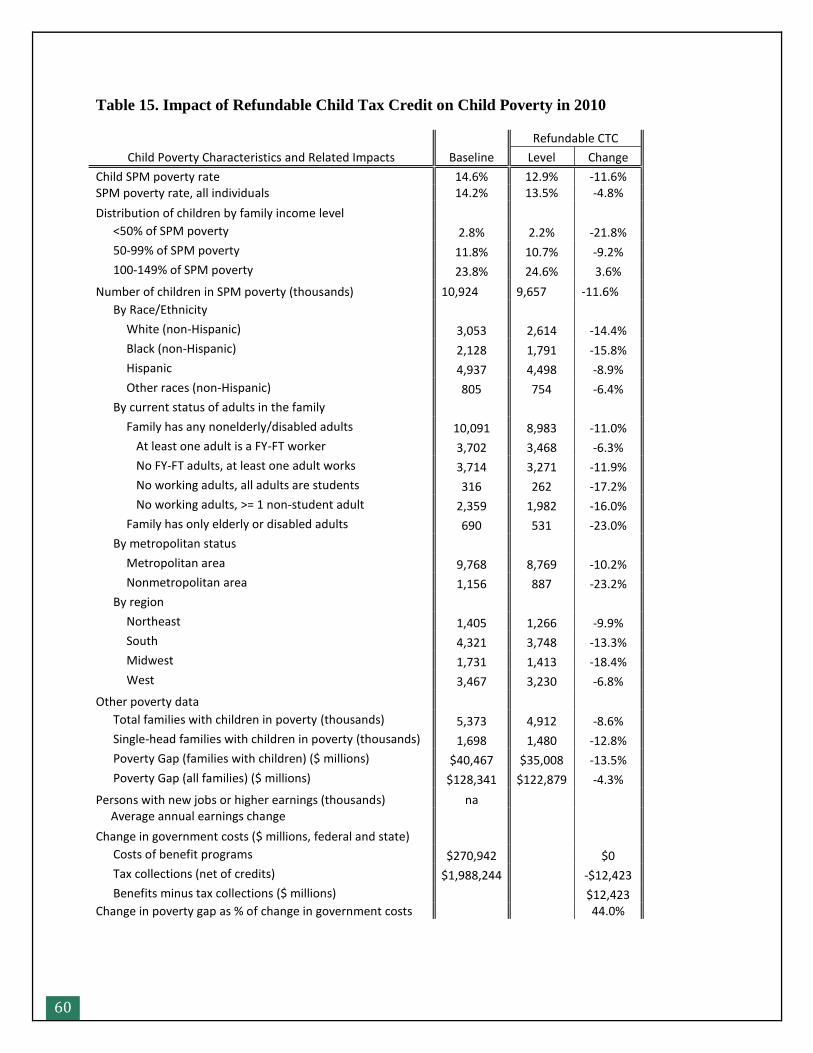
60
Table 15. Impact of Refundable Child Tax Credit on Child Poverty in 2010
Child Poverty Characteristics and Related Impacts Baseline
Refundable CTC
Level Change
Child SPM poverty rate 14.6% 12.9% -11.6% SPM poverty rate, all individuals 14.2% 13.5% -4.8%
Distribution of children by family income level
<50% of SPM poverty 2.8% 2.2% -21.8%
50-99% of SPM poverty 11.8% 10.7% -9.2%
100-149% of SPM poverty 23.8% 24.6% 3.6%
Number of children in SPM poverty (thousands) 10,924 9,657 -11.6%
By Race/Ethnicity
White (non-Hispanic) 3,053 2,614 -14.4%
Black (non-Hispanic) 2,128 1,791 -15.8%
Hispanic 4,937 4,498 -8.9%
Other races (non-Hispanic) 805 754 -6.4%
By current status of adults in the family
Family has any nonelderly/disabled adults 10,091 8,983 -11.0%
At least one adult is a FY-FT worker 3,702 3,468 -6.3%
No FY-FT adults, at least one adult works 3,714 3,271 -11.9%
No working adults, all adults are students 316 262 -17.2%
No working adults, >= 1 non-student adult 2,359 1,982 -16.0%
Family has only elderly or disabled adults 690 531 -23.0%
By metropolitan status
Metropolitan area 9,768 8,769 -10.2%
Nonmetropolitan area 1,156 887 -23.2%
By region
Northeast 1,405 1,266 -9.9%
South 4,321 3,748 -13.3%
Midwest 1,731 1,413 -18.4%
West 3,467 3,230 -6.8%
Other poverty data
Total families with children in poverty (thousands) 5,373 4,912 -8.6%
Single-head families with children in poverty (thousands) 1,698 1,480 -12.8%
Poverty Gap (families with children) ($ millions) $40,467 $35,008 -13.5%
Poverty Gap (all families) ($ millions) $128,341 $122,879 -4.3%
Persons with new jobs or higher earnings (thousands) na Average annual earnings change
Change in government costs ($ millions, federal and state)
Costs of benefit programs $270,942 $0
Tax collections (net of credits) $1,988,244 -$12,423
Benefits minus tax collections ($ millions) $12,423 Change in poverty gap as % of change in government costs 44.0%
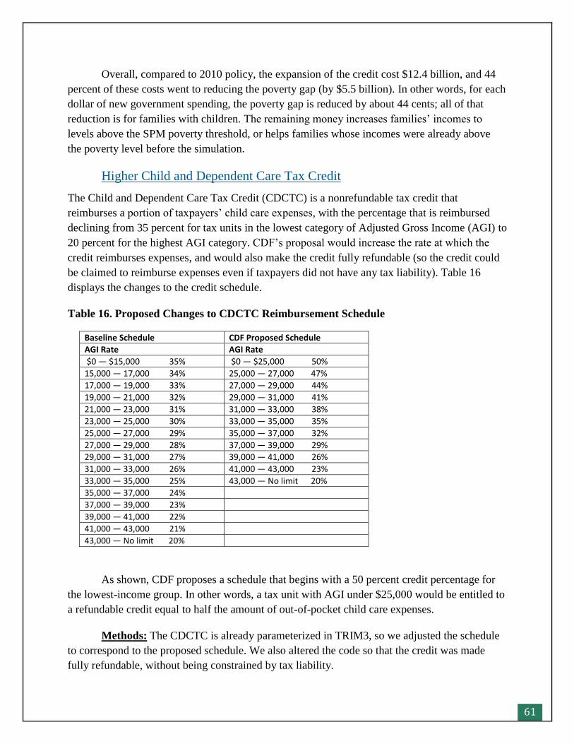
61
Overall, compared to 2010 policy, the expansion of the credit cost $12.4 billion, and 44
percent of these costs went to reducing the poverty gap (by $5.5 billion). In other words, for each
dollar of new government spending, the poverty gap is reduced by about 44 cents; all of that
reduction is for families with children. The remaining money increases families’ incomes to
levels above the SPM poverty threshold, or helps families whose incomes were already above
the poverty level before the simulation.
Higher Child and Dependent Care Tax Credit
The Child and Dependent Care Tax Credit (CDCTC) is a nonrefundable tax credit that
reimburses a portion of taxpayers’ child care expenses, with the percentage that is reimbursed
declining from 35 percent for tax units in the lowest category of Adjusted Gross Income (AGI) to
20 percent for the highest AGI category. CDF’s proposal would increase the rate at which the
credit reimburses expenses, and would also make the credit fully refundable (so the credit could
be claimed to reimburse expenses even if taxpayers did not have any tax liability). Table 16
displays the changes to the credit schedule.
Table 16. Proposed Changes to CDCTC Reimbursement Schedule
Baseline Schedule CDF Proposed Schedule
AGI Rate AGI Rate
$0 — $15,000 35% $0 — $25,000 50%
15,000 — 17,000 34% 25,000 — 27,000 47%
17,000 — 19,000 33% 27,000 — 29,000 44%
19,000 — 21,000 32% 29,000 — 31,000 41%
21,000 — 23,000 31% 31,000 — 33,000 38%
23,000 — 25,000 30% 33,000 — 35,000 35%
25,000 — 27,000 29% 35,000 — 37,000 32%
27,000 — 29,000 28% 37,000 — 39,000 29%
29,000 — 31,000 27% 39,000 — 41,000 26%
31,000 — 33,000 26% 41,000 — 43,000 23%
33,000 — 35,000 25% 43,000 — No limit 20%
35,000 — 37,000 24%
37,000 — 39,000 23%
39,000 — 41,000 22%
41,000 — 43,000 21%
43,000 — No limit 20%
As shown, CDF proposes a schedule that begins with a 50 percent credit percentage for
the lowest-income group. In other words, a tax unit with AGI under $25,000 would be entitled to
a refundable credit equal to half the amount of out-of-pocket child care expenses.
Methods: The CDCTC is already parameterized in TRIM3, so we adjusted the schedule
to correspond to the proposed schedule. We also altered the code so that the credit was made
fully refundable, without being constrained by tax liability.

62
In addition to simulating a static estimate of the credit, we simulated the credit with
employment effects. For parents who must pay for child care, reimbursing a portion of child care
expenses essentially increases the economic gain for working, and the economic literature
suggests that in general, labor supply increases when the gains to work increase. While there is a
relatively sparse literature on the employment effects of the CDCTC, the available studies
(Averett, Peters, and Waldman 1997 and Miller and Mumford 2011) treat the credit as simply
reducing the price of childcare and compute elasticities of labor supply with respect to this
reduced price. We thus based the employment effects for the credit on the change in net child
care price, using the same method and elasticity used for the child care subsidy expansion. In
brief, we assume that a parent’s probability of taking a job equals 0.3 times the percentage
reduction in the cost of child care. Since these are parents who are not currently working (and not
currently using child care), we use imputation equations to estimate if they would pay for child
care and if so, how much. (Further details are provided below in the discussion of labor supply
impacts for the CCDF expansion.) We also assumed that there would be no increase in funding
for CCDF subsidies to accompany the CDCTC increase, meaning no new families would receive
child care subsidies.
Results: When the CDCTC expansion is modeled without employment effects, the
number of tax units taking the credit increases by 1.3 million (22 percent) due to the credit
becoming refundable, and the total amount of credit increases by $1.6 billion (45 percent) due to
a combination of refundability and the increased credit percentage (table C3.4b). Due to
secondary impacts on other aspects of federal taxes and also impacts on state income taxes, total
tax liability falls by $1.7 billion.
The simulation of employment effects results in 101,000 new jobs being modeled. All of
the new workers are parents who would benefit from the CDCTC, and who would benefit more
from the modified CDCCTC than from the actual credit. With the new workers also taking the
CDCTC, the aggregate credit increases by $1.7 billion relative to the baseline. Aggregate tax
liability falls by $2 billion in this scenario, and there is a $0.4 billion reduction in spending on
government benefits due to the fact that some families now have new earnings. On net,
government costs increase by $1.6 billion. (The increased costs from more credits being claimed
by new workers were more than offset by the reductions in transfer program benefits for those
families.)
Despite the substantial percentage impacts on the CDCTC credit, the expansion had
relatively low impacts on SPM poverty (table 17). Child poverty is reduced by 0.6 percent
without employment effects and by 1.3 percent when employment effects are included. The
poverty gap for families with children is reduced by $520 million, or 1.3 percent; there was no
impact on the poverty gap for families without children.
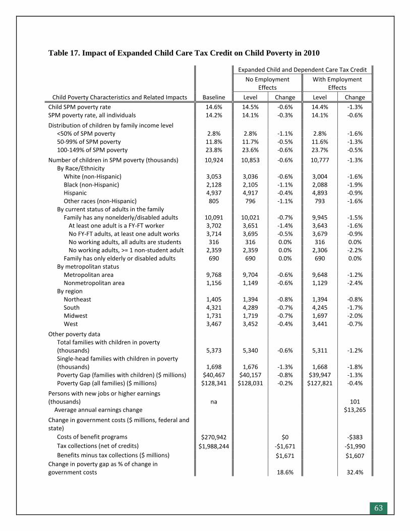
63
Table 17. Impact of Expanded Child Care Tax Credit on Child Poverty in 2010
Child Poverty Characteristics and Related Impacts Baseline
Expanded Child and Dependent Care Tax Credit
No Employment Effects
With Employment Effects
Level Change Level Change
Child SPM poverty rate 14.6% 14.5% -0.6% 14.4% -1.3% SPM poverty rate, all individuals 14.2% 14.1% -0.3% 14.1% -0.6%
Distribution of children by family income level <50% of SPM poverty 2.8% 2.8% -1.1% 2.8% -1.6% 50-99% of SPM poverty 11.8% 11.7% -0.5% 11.6% -1.3% 100-149% of SPM poverty 23.8% 23.6% -0.6% 23.7% -0.5%
Number of children in SPM poverty (thousands) 10,924 10,853 -0.6% 10,777 -1.3% By Race/Ethnicity White (non-Hispanic) 3,053 3,036 -0.6% 3,004 -1.6% Black (non-Hispanic) 2,128 2,105 -1.1% 2,088 -1.9% Hispanic 4,937 4,917 -0.4% 4,893 -0.9% Other races (non-Hispanic) 805 796 -1.1% 793 -1.6% By current status of adults in the family Family has any nonelderly/disabled adults 10,091 10,021 -0.7% 9,945 -1.5% At least one adult is a FY-FT worker 3,702 3,651 -1.4% 3,643 -1.6% No FY-FT adults, at least one adult works 3,714 3,695 -0.5% 3,679 -0.9% No working adults, all adults are students 316 316 0.0% 316 0.0% No working adults, >= 1 non-student adult 2,359 2,359 0.0% 2,306 -2.2% Family has only elderly or disabled adults 690 690 0.0% 690 0.0% By metropolitan status Metropolitan area 9,768 9,704 -0.6% 9,648 -1.2% Nonmetropolitan area 1,156 1,149 -0.6% 1,129 -2.4% By region Northeast 1,405 1,394 -0.8% 1,394 -0.8% South 4,321 4,289 -0.7% 4,245 -1.7% Midwest 1,731 1,719 -0.7% 1,697 -2.0% West 3,467 3,452 -0.4% 3,441 -0.7%
Other poverty data
Total families with children in poverty (thousands) 5,373 5,340 -0.6% 5,311 -1.2%
Single-head families with children in poverty (thousands) 1,698 1,676 -1.3% 1,668 -1.8%
Poverty Gap (families with children) ($ millions) $40,467 $40,157 -0.8% $39,947 -1.3% Poverty Gap (all families) ($ millions) $128,341 $128,031 -0.2% $127,821 -0.4%
Persons with new jobs or higher earnings (thousands) na 101
Average annual earnings change $13,265
Change in government costs ($ millions, federal and state)
Costs of benefit programs $270,942 $0 -$383
Tax collections (net of credits) $1,988,244 -$1,671 -$1,990
Benefits minus tax collections ($ millions) $1,671 $1,607 Change in poverty gap as % of change in government costs 18.6% 32.4%
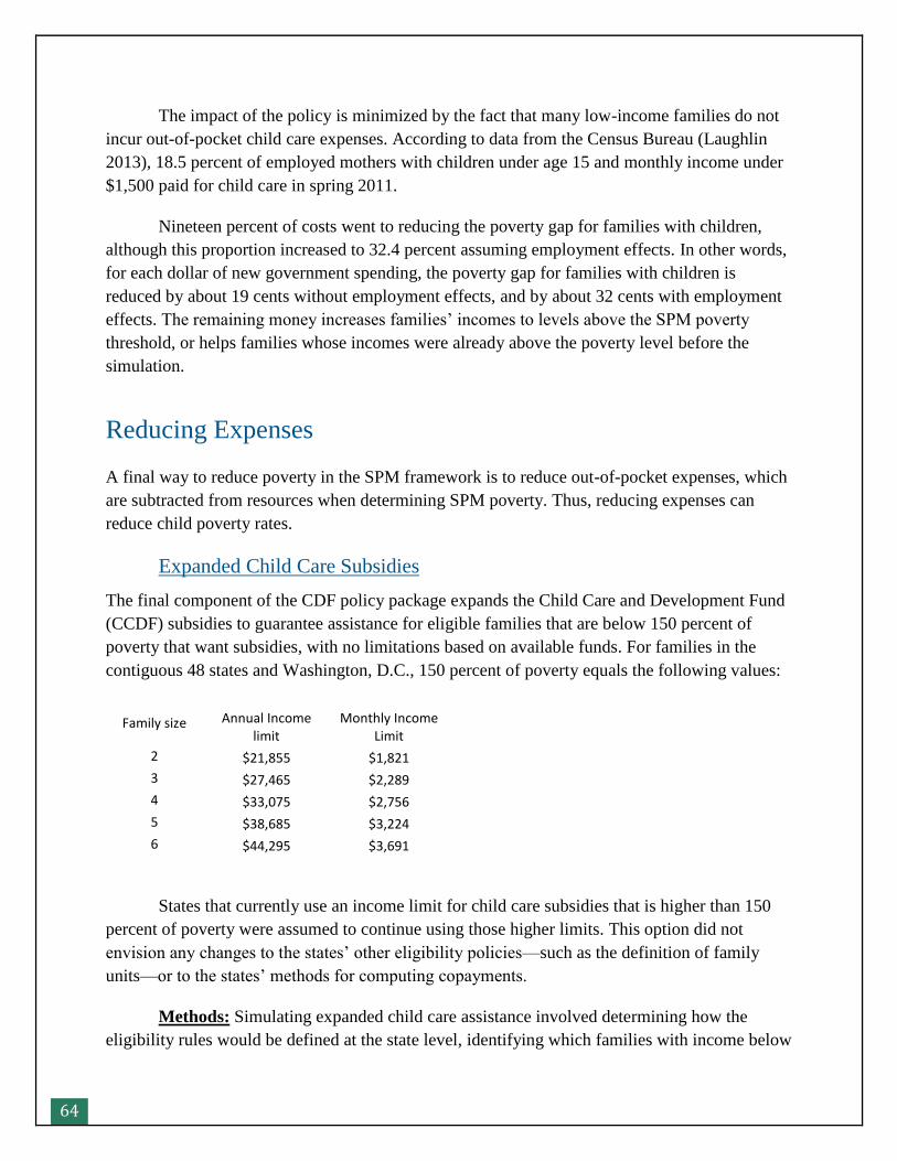
64
The impact of the policy is minimized by the fact that many low-income families do not
incur out-of-pocket child care expenses. According to data from the Census Bureau (Laughlin
2013), 18.5 percent of employed mothers with children under age 15 and monthly income under
$1,500 paid for child care in spring 2011.
Nineteen percent of costs went to reducing the poverty gap for families with children,
although this proportion increased to 32.4 percent assuming employment effects. In other words,
for each dollar of new government spending, the poverty gap for families with children is
reduced by about 19 cents without employment effects, and by about 32 cents with employment
effects. The remaining money increases families’ incomes to levels above the SPM poverty
threshold, or helps families whose incomes were already above the poverty level before the
simulation.
Reducing Expenses
A final way to reduce poverty in the SPM framework is to reduce out-of-pocket expenses, which
are subtracted from resources when determining SPM poverty. Thus, reducing expenses can
reduce child poverty rates.
Expanded Child Care Subsidies
The final component of the CDF policy package expands the Child Care and Development Fund
(CCDF) subsidies to guarantee assistance for eligible families that are below 150 percent of
poverty that want subsidies, with no limitations based on available funds. For families in the
contiguous 48 states and Washington, D.C., 150 percent of poverty equals the following values:
Family size Annual Income limit
Monthly Income Limit
2 $21,855 $1,821
3 $27,465 $2,289
4 $33,075 $2,756
5 $38,685 $3,224
6 $44,295 $3,691
States that currently use an income limit for child care subsidies that is higher than 150
percent of poverty were assumed to continue using those higher limits. This option did not
envision any changes to the states’ other eligibility policies—such as the definition of family
units—or to the states’ methods for computing copayments.
Methods: Simulating expanded child care assistance involved determining how the
eligibility rules would be defined at the state level, identifying which families with income below
65
150 percent of poverty who would want to begin receiving child care assistance, and computing
the value of the subsidy. In a second version of the simulation, we also modeled the effects this
child care guarantee would have on employment.
The existing child care subsidy program follows broad federal guidelines, but most of the
policies affecting eligibility, family payments, and provider payments are established at the state
level. While this policy proposal guarantees assistance for families with income below 150
percent of the poverty guidelines, in reality states may set their income eligibility limits higher
than this—up to 85 percent of the state median income—and in 2010 only eight states set their
limits below 150 percent of poverty. States are also given substantial leeway in establishing
policies for work requirements (the minimum hours per week required for a family to be eligible
for subsidies), defining the assistance unit, and determining what types of income are counted.
For example, one of the states with an income limit slightly below 150 percent of poverty allows
families to disregard a portion of their earnings before determining eligibility, thus making their
eligibility policy more generous than it would appear based on the income limit alone. Because
of these complexities, the simulation left current state-specific policies in place, but imposed a
national-level policy that any family that was eligible according to the state rules and that had
income under 150 percent of poverty would be guaranteed a subsidy.
To model the guarantee, we identified eligible families with income under 150 percent of
poverty that were not previously receiving CCDF-funded subsidies. In reality, not all families
would choose to use the subsidy, even when eligible for assistance. For example, families might
not take up the subsidy because they have access to less expensive child care arrangements, such
as having a child cared for by a grandmother who does not ask for payment. In order to account
for the fact that not all eligible families would choose to use assistance, we only selected families
to take advantage of the new subsidy guarantee (and begin receiving a subsidy) if they reported
paying child care expenses in the CPS-ASEC survey data. This represents a lower bound on the
cost of the guarantee, since some families currently using free or low-cost child care might
choose to take a subsidy—even if the copay would increase their out-of-pocket expenses—in
order to obtain more formal care for their children. Note that all families with a child care
subsidy in the baseline simulation were modeled to retain the subsidy.
In order to assess the policy package and its potential costs, the simulation must estimate
the amount that families are required to pay (referred to as the family’s copayment) and the total
value of the child care. In both the baseline simulation and this simulation, we first
probabilistically assign a type of child care (informal, family day care, center based care) using
administrative data on actual subsidy recipients. We then assume that each family locates child
care with a full cost equal to exactly the “maximum rates” that their state paid for that type of
care in 2010. Finally, we computed the copayments, using the same state-by-state policies used
in the baseline simulation. The cost of each family’s subsidy (the government’s cost for that
66
family’s subsidy) equals the maximum rates (summed across the family’s children) minus the
family’s copayment.
One consideration of expanding child care assistance is the potential impact that access to
child care may have on employment. Summaries of the literature (Blau, 2003 and Ziliak et al.
2008) find considerable uncertainty about the effects of child care costs on employment, with
modal elasticities of -0.3 to -0.4 for single mothers and lower estimates for married mothers. This
implies that a 1 percent reduction in child care costs would correspond to a 0.3 to 0.4 percent
increase in employment for single mothers. However, more recent studies (Fitzpatrick 2012,
Herbst 2010, and Tekin 2007) find smaller effects, which some authors have attributed to the
economy-wide increases in mothers’ labor supply over time. Additionally, two recent large-scale
randomized experiments in Illinois and Washington state (Michalopoulos, Lundquist and
Castells 2010 and Michalopoulos 2010) found no effects of increased child care subsidy
eligibility or reduced copayments on employment.
In light of this uncertainty, we modeled an employment effect at a 0.3 elasticity to
provide a comparison to the simulation without employment effects. For each family with non-
working adults and children under 13 (the age limit for CCDF eligibility for children without
special needs), we computed the child care expenses that the family would incur if the non-
working adults took a job at the minimum wage, without any expansion to child care subsidies.
(Disabled adults and students were excluded from this calculation.)52 We next computed for each
family the childcare expenses that would be incurred by starting work after the expansion of the
subsidy program. For this second calculation, we assumed that all eligible families would
participate in child care subsidies; families that were subsidized had a child care expense equal to
their simulated copayment. We then computed the probability of taking a new job as the
percentage change in child care expenses times the elasticity of 0.3. Thus, a family who saw their
child care expenses upon taking a job fall from a positive value to zero (a 100 percent reduction
in expenses) would have a 30 percent chance of taking a new job, while a family that saw a 50
percent reduction in expenses would have a 15 percent chance of taking a new job.
We compared the probabilities of taking a job to a random number for each family, to
determine whether the family head would begin work (families where both the head and spouse
did not work were excluded, as we assumed childcare was not a constraint on work for these
families). Families that began work were assigned jobs at the minimum wage with hours based
on the characteristics of jobs held by workers in SPM poverty in the 2010 baseline (as described
52 These expenses were estimated based on regression equations calculated from SIPP data using a large number of
family and income characteristics, and calibrated to produce the same level of child care expenses as the CY 2010
CPS-ASEC data. For this particular purpose, we assumed all families would have a non-zero expense, to provide an
estimate for each family of the price the family would pay for child care given that they pay some amount (reflecting
the implicit value of the childcare subsidy to each family). We then subtracted the value of the baseline CDCTC (as
this tax credit offsets child care expenses) to arrive at a final figure for expenses that the family would incur if adults
began to work.

67
in the EITC simulation, above). Any parent who was simulated to start to work due to the
availability of the subsidy was also simulated to enroll in the subsidy program. (Note that for
these families, child care expenses were previously $0, and now they may be a positive amount
due to copayments; however, the copay expense will presumably be offset by the new earnings.)
Results: In the simulation of the CCDF guarantee without employment effects, an
additional 0.6 million families begin receiving subsidies, increasing the CCDF caseload by 62
percent and increasing the aggregate cost of subsidies by $3.9 billion (57 percent) (table C3.5a).
The average monthly subsidy is $561—just slightly below the monthly subsidy in the baseline,
$567. Differences in the average subsidy amounts for newly subsidized families versus families
subsidized in the baseline could be due to a different distribution of the newly subsidized units
across states, since states vary in their reimbursement rates and copayment policies.
The expanded child care subsidies have some secondary impacts on programs. Since
SNAP, TANF, and housing subsidies all include child care deductions, benefits paid by those
programs all drop slightly, due to the fact that some families now have lower child care
expenses. The amount of child and dependent care credit in the federal income tax system also
decreases slightly. These changes offset some of the costs of the new subsidies, and aggregate
government costs increase by $3.6 billion (table 18).
The net impact of the subsidy guarantee, in the absence of employment effects, is that
child poverty is reduced from the baseline level of 14.6 percent by a very small amount, to 14.5
percent. The impact is relatively similar across races, as well as in metropolitan and
nonmetropolitan areas. The percentage reduction is larger (1.4 percent) for children in families
with full-year full-time workers, and there is no impact in families with nonelderly nondisabled
adults who are out of the labor force and not students. There is a 1.1 percent reduction for
children in families where the adults are students, since CCDF is also available for students.
When the employment effects are included, 358,000 people are simulated to take new
jobs, with average annual earnings of $12,523. All of the new workers are modeled to take
CCDF subsidies, bringing the total program caseload to 1.9 million (an increase of 97 percent
from the baseline) and the total value of subsidies to $13.6 billion (an increase of 102 percent).
Factoring in reductions in benefits due to new earnings and due to lower child care expenses, and
an overall decrease in tax revenues (as the increase in refundable tax credits on new earnings
exceeds the taxes on the new earnings) total government costs increase by $5.3 billion.
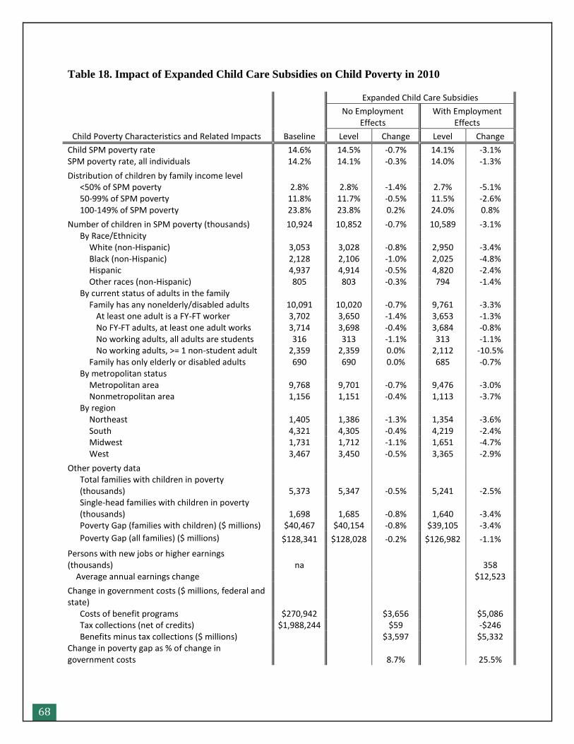
68
Table 18. Impact of Expanded Child Care Subsidies on Child Poverty in 2010
Child Poverty Characteristics and Related Impacts Baseline
Expanded Child Care Subsidies
No Employment Effects
With Employment Effects
Level Change Level Change
Child SPM poverty rate 14.6% 14.5% -0.7% 14.1% -3.1% SPM poverty rate, all individuals 14.2% 14.1% -0.3% 14.0% -1.3%
Distribution of children by family income level
<50% of SPM poverty 2.8% 2.8% -1.4% 2.7% -5.1%
50-99% of SPM poverty 11.8% 11.7% -0.5% 11.5% -2.6%
100-149% of SPM poverty 23.8% 23.8% 0.2% 24.0% 0.8%
Number of children in SPM poverty (thousands) 10,924 10,852 -0.7% 10,589 -3.1%
By Race/Ethnicity
White (non-Hispanic) 3,053 3,028 -0.8% 2,950 -3.4%
Black (non-Hispanic) 2,128 2,106 -1.0% 2,025 -4.8%
Hispanic 4,937 4,914 -0.5% 4,820 -2.4%
Other races (non-Hispanic) 805 803 -0.3% 794 -1.4%
By current status of adults in the family
Family has any nonelderly/disabled adults 10,091 10,020 -0.7% 9,761 -3.3%
At least one adult is a FY-FT worker 3,702 3,650 -1.4% 3,653 -1.3%
No FY-FT adults, at least one adult works 3,714 3,698 -0.4% 3,684 -0.8%
No working adults, all adults are students 316 313 -1.1% 313 -1.1%
No working adults, >= 1 non-student adult 2,359 2,359 0.0% 2,112 -10.5%
Family has only elderly or disabled adults 690 690 0.0% 685 -0.7%
By metropolitan status
Metropolitan area 9,768 9,701 -0.7% 9,476 -3.0%
Nonmetropolitan area 1,156 1,151 -0.4% 1,113 -3.7%
By region
Northeast 1,405 1,386 -1.3% 1,354 -3.6%
South 4,321 4,305 -0.4% 4,219 -2.4%
Midwest 1,731 1,712 -1.1% 1,651 -4.7%
West 3,467 3,450 -0.5% 3,365 -2.9%
Other poverty data
Total families with children in poverty (thousands) 5,373 5,347 -0.5% 5,241 -2.5%
Single-head families with children in poverty (thousands) 1,698 1,685 -0.8% 1,640 -3.4%
Poverty Gap (families with children) ($ millions) $40,467 $40,154 -0.8% $39,105 -3.4%
Poverty Gap (all families) ($ millions) $128,341 $128,028 -0.2% $126,982 -1.1%
Persons with new jobs or higher earnings (thousands) na
358 Average annual earnings change $12,523
Change in government costs ($ millions, federal and state)
Costs of benefit programs $270,942 $3,656 $5,086
Tax collections (net of credits) $1,988,244 $59 -$246
Benefits minus tax collections ($ millions) $3,597 $5,332
Change in poverty gap as % of change in government costs 8.7% 25.5%
69
In the employment-effects scenario, the child poverty rate is reduced to 14.1 percent (a
reduction of 3.1 percent). Relative to the scenario without employment effects, an additional
263,000 children are raised out of SPM poverty; this suggests that a substantial portion of the
358,000 new workers were able to raise their families out of poverty through the new job
combined with child care subsidies The reduction in the poverty gap for families with children is
$1.4 billion, or 3.4 percent; families without children are unaffected.
The poverty impacts of the child care subsidy expansion are small compared to other
program changes proposed in the CDF package. One factor is that the child care subsidy policy
only helps families with parents who are working or who are students, and only helps families
with children under age 13. Also, the amount of the subsidy varies based on a number of factors
(e.g., the maximum reimbursement rate may be lower for parents working part-time) and on its
own the value of the subsidy may not be high enough to pull a family out of poverty. Finally, as
mentioned above, we only simulated an eligible family to newly receive a subsidy if the family
had child care expenses in the baseline simulation, and only a minority of low-income working
families with children pay for child care.
Another reason for the limited impact on SPM poverty is related to the way in which the
SPM treats child care costs. Child care is reflected in the SPM through expense amounts;
specifically, child care expenses are subtracted from other resources. When a family has a
subsidy, the family pays only a portion of the total cost (the copayment), and some families owe
no copayment. Therefore, the SPM picks up an economic benefit to receiving a child care
subsidy to the extent that a family’s out-of-pocket child care expenses are lowered, relative to the
unsubsidized expenses before having a subsidy. However, if a family previously paying $200 per
month in unsubsidized child care expense for an informal arrangement begins to receive a CCDF
subsidy and pays a copayment that is also $200 per month, there is no change in the family’s
economic well-being as measured by the SPM, even though the economic value of the two
arrangements might be quite different. If a low-income family previously had low child care
expenses, the reduction in expense when taking a subsidy could be relatively small. The subsidy
may increase the quality of the child care that the family can access, but the impact on the
family’s expenses may not be large.
The change in the poverty gap as a percentage of the change in government costs is 8.7
percent without employment effects and 25.5 percent with employment effects. In other words,
for each dollar of new government spending, the poverty gap is reduced by about 9 cents without
employment effects and by 25.5 cents with employment effects (and all of the poverty gap
reduction occurs for families with children). As mentioned above, the cost to the government of
providing a subsidy equals the assumed full value of the child care being provided minus the
copayment paid by the family. However, the economic benefit to the family is the difference
between the family’s unsubsidized payment (which could be much less than the full value of the

70
new care) minus the copayment. Thus, the government’s costs include the increased value of
child care being provided while the poverty impacts reflect only families’ out-of-pocket costs.
71
Combining Policies
After running simulations of the effects of each policy if enacted individually, we simulated the
effects of the policies on poverty when enacted together in several combinations. When policies
are combined, the antipoverty impact may be smaller than the sum of the individual impacts—if
the same children would be removed from poverty by any one of multiple policies; or larger than
the sum of the individual impacts—if many children are removed from poverty only by a
combination of policies.
Minimum Wage and EITC
We first simulated the effects of the EITC increase (with employment effects) in combination
with the minimum wage increase (including spillover and job loss effects).
Methods: We assumed that individuals who were induced to work by the higher EITC
would receive jobs at the higher minimum wage; however, fewer of these jobs would be awarded
in total, since some of those jobs would not be available after job loss was assumed. In other
words, we applied the same probability of job loss to individuals who started work due to the
EITC as to other minimum wage workers.
Results: Enacting both the minimum wage and EITC policies reduced child poverty by
12.4 percent, to a rate of 12.8 percent. The number of children removed from poverty—1.36
million—is just slightly below the sum of those removed from poverty by the individual policies
(0.96 million due to the EITC expansion with employment effects and 0.43 million due to the
minimum wage with spillover and job loss, for a total of 1.39 million) (table 19). This suggests
that the number of children who would be brought out of poverty by either one of the policies is
only slightly larger than the number of children who are only brought out of poverty by the
combination of the two policies.
The effects were strongest for black children (a 16.5 percent reduction), children in
families with no working adults (a 15.5 percent reduction), and single-headed families with
children (a 14.9 percent reduction). A total of 28.0 million people saw either new jobs or higher
earnings from the policy, with an average increase in earnings of $1,864, while 258,000 were
simulated to lose jobs. The policy overall was simulated to result in budgetary savings, as the
higher minimum wage reduced the cost of benefit programs by $3.2 billion, and the cost of the
higher EITC was offset by $5.1 billion in increased tax revenues from the higher minimum
wage, resulting in a net $8.3 billion savings to the government. (We do not present the cost
results relative to the poverty gap because this combination of policies resulted in no net costs.
The poverty gap reduction results primarily from the increased wages, the cost of which is
presumably borne by private businesses.)
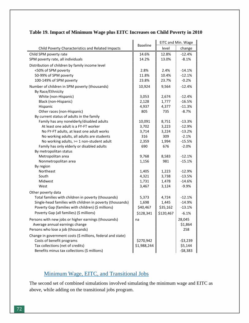
72
Table 19. Impact of Minimum Wage plus EITC Increases on Child Poverty in 2010
Child Poverty Characteristics and Related Impacts Baseline
EITC and Min. Wage
level change
Child SPM poverty rate 14.6% 12.8% -12.4% SPM poverty rate, all individuals 14.2% 13.0% -8.1%
Distribution of children by family income level
<50% of SPM poverty 2.8% 2.4% -14.1%
50-99% of SPM poverty 11.8% 10.4% -12.1%
100-149% of SPM poverty 23.8% 23.7% -0.2%
Number of children in SPM poverty (thousands) 10,924 9,564 -12.4%
By Race/Ethnicity
White (non-Hispanic) 3,053 2,674 -12.4%
Black (non-Hispanic) 2,128 1,777 -16.5%
Hispanic 4,937 4,377 -11.3%
Other races (non-Hispanic) 805 735 -8.7%
By current status of adults in the family
Family has any nonelderly/disabled adults 10,091 8,751 -13.3%
At least one adult is a FY-FT worker 3,702 3,223 -12.9%
No FY-FT adults, at least one adult works 3,714 3,224 -13.2%
No working adults, all adults are students 316 309 -2.1%
No working adults, >= 1 non-student adult 2,359 1,994 -15.5%
Family has only elderly or disabled adults 690 676 -2.0%
By metropolitan status
Metropolitan area 9,768 8,583 -12.1%
Nonmetropolitan area 1,156 981 -15.1%
By region
Northeast 1,405 1,223 -12.9%
South 4,321 3,738 -13.5%
Midwest 1,731 1,478 -14.6%
West 3,467 3,124 -9.9%
Other poverty data
Total families with children in poverty (thousands) 5,373 4,724 -12.1%
Single-head families with children in poverty (thousands) 1,698 1,445 -14.9%
Poverty Gap (families with children) ($ millions) $40,467 $35,162 -13.1%
Poverty Gap (all families) ($ millions) $128,341 $120,467 -6.1%
Persons with new jobs or higher earnings (thousands) na 28,045 Average annual earnings change $1,864
Persons who lose a job (thousands) 258
Change in government costs ($ millions, federal and state)
Costs of benefit programs $270,942 -$3,239
Tax collections (net of credits) $1,988,244 $5,144
Benefits minus tax collections ($ millions) -$8,383
Minimum Wage, EITC, and Transitional Jobs
The second set of combined simulations involved simulating the minimum wage and EITC as
above, while adding on the transitional jobs program.
73
Methods: When adding the transitional jobs to the policies above, it was necessary to
consider the ordering of different types of job changes—new TJ jobs, new jobs due to the EITC,
and job loss due to the minimum wage. We assumed that some individuals who were simulated
to take transitional jobs in the individual simulation of that policy did not do so in this
simulation, as they were already assumed to take an unsubsidized job due to the EITC expansion.
Additionally, we assumed that individuals who lost their jobs due to the minimum wage would
not take a transitional job (to reflect that a higher minimum wage could lead to a small amount of
additional slack in the labor market, even in the presence of a TJ program). The transitional jobs
were provided at the higher minimum wage.
Results: Enacting the three policies in concert reduced child poverty by 23.4 percent
(table 20). A total of 2.6 million children were removed from poverty, almost exactly the same as
the sum of antipoverty impacts from the individual policies. There was also a 30.1 percent
reduction in deep poverty. The poverty gap for families with children fell by $10.9 billion, or 27
percent. Including families without children, the poverty gap fell by $13.5 billion (since some of
the families that benefit from the higher minimum wage do not have children). The groups most
helped by the three combined policies were black children (with a 29.6 percent reduction in
poverty) and children in families with no working adults and at least one non-student adult (with
a 40 percent reduction).
Overall, 30.4 million people were estimated to gain jobs or higher earnings, with an
average annual gain of $2,831, and 258,000 were simulated to lose jobs (as in the previous
simulation). The government would expend $29.6 billion on the transitional jobs program after
subtracting reduced transfer program benefits. Tax collections would be decreased by the
expanded EITC but increased by payroll and income taxes owed on new jobs, for a net increase
of $11.1 billion in tax collections, giving an overall government cost of the combined policies of
$18.5 billion.
The change in the poverty gap (over all families) as a percentage of the change in
government costs for the simulated programs is 72.9 percent. In other words, for each dollar of
new government spending on transitional jobs or the expanded EITC, the poverty gap is reduced
by about 73 cents, when combined with the minimum wage increase. The ratio is very high
because the cost of the increased wages from the minimum wage change play a large role in
reducing the poverty gap (the numerator of the ratio), but they are not reflected in government
costs (the denominator).
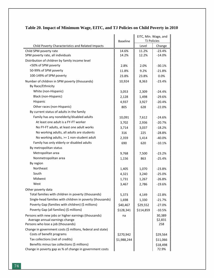
74
Table 20. Impact of Minimum Wage, EITC, and TJ Policies on Child Poverty in 2010
Child Poverty Characteristics and Related Impacts
Baseline
EITC, Min. Wage, and TJ Policies
Level Change
Child SPM poverty rate 14.6% 11.2% -23.4% SPM poverty rate, all individuals 14.2% 12.2% -14.0%
Distribution of children by family income level
<50% of SPM poverty 2.8% 2.0% -30.1%
50-99% of SPM poverty 11.8% 9.2% -21.8%
100-149% of SPM poverty 23.8% 23.8% 0.0%
Number of children in SPM poverty (thousands) 10,924 8,363 -23.4%
By Race/Ethnicity
White (non-Hispanic) 3,053 2,309 -24.4%
Black (non-Hispanic) 2,128 1,498 -29.6%
Hispanic 4,937 3,927 -20.4%
Other races (non-Hispanic) 805 628 -22.0%
By current status of adults in the family
Family has any nonelderly/disabled adults 10,091 7,612 -24.6%
At least one adult is a FY-FT worker 3,702 2,936 -20.7%
No FY-FT adults, at least one adult works 3,714 3,037 -18.2%
No working adults, all adults are students 316 225 -28.8%
No working adults, >= 1 non-student adult 2,359 1,414 -40.0%
Family has only elderly or disabled adults 690 620 -10.1%
By metropolitan status
Metropolitan area 9,768 7,500 -23.2%
Nonmetropolitan area 1,156 863 -25.4%
By region
Northeast 1,405 1,070 -23.8%
South 4,321 3,240 -25.0%
Midwest 1,731 1,267 -26.8%
West 3,467 2,786 -19.6%
Other poverty data
Total families with children in poverty (thousands) 5,373 4,149 -22.8%
Single-head families with children in poverty (thousands) 1,698 1,330 -21.7%
Poverty Gap (families with children) ($ millions) $40,467 $29,552 -27.0%
Poverty Gap (all families) ($ millions) $128,341 $114,859 -10.5%
Persons with new jobs or higher earnings (thousands) na 30,389 Average annual earnings change $2,831
Persons who lose a job (thousands) 258
Change in government costs ($ millions, federal and state)
Costs of benefit programs $270,942 $29,564
Tax collections (net of credits) $1,988,244 $11,066
Benefits minus tax collections ($ millions) $18,498 Change in poverty gap as % of change in government costs 72.9%
75
All Policies Combined
The final simulation combined all of the individual policies already discussed, as follows:
Increases to cash income:
Minimum wage increased to a level of $10.10 in 2014 dollars for covered workers, and 70
percent of that level for tipped workers
Transitional jobs program with a participation rate of 25 percent for unemployed individuals
with the lowest family incomes; in this simulation, the jobs pay the increased minimum wage
A full pass-through and disregard of child support income by the TANF program, and a
partial disregard of child support by the SNAP program
Increased in-kind benefits:
Expanded access to housing vouchers for low-income households with children
Increased SNAP benefits
Reduced taxes:
Expanded Earned Income Tax Credit
Fully refundable Child Tax Credit
Increased Child and Dependent Care Tax Credit (CDCTC)
Reduced expenses:
Expanded access to child care subsidies for low-income families with children under age 13
Methods: The simulations were all modeled in combination, capturing all of the
interactions and secondary impacts. For the policies that were simulated both with and without
employment effects, this combination simulation included those effects. We assumed that
anyone who would have been modeled to start to work due to the EITC, CTC, or child care
subsidy expansion in the individual policy simulations would also have started to work in this
combination simulation. We also included the spillover effects from the minimum wage increase
and a small amount of job loss, as discussed earlier. Some workers previously selected as taking
a transitional job did not take a TJ in this simulation, because they were modeled as already
working at an unsubsidized job due to another policy.
Results: The combination of the policies greatly reduces child poverty. The SPM poverty
rate for children falls from the baseline level of 14.6 percent to 5.8 percent, a reduction of 60
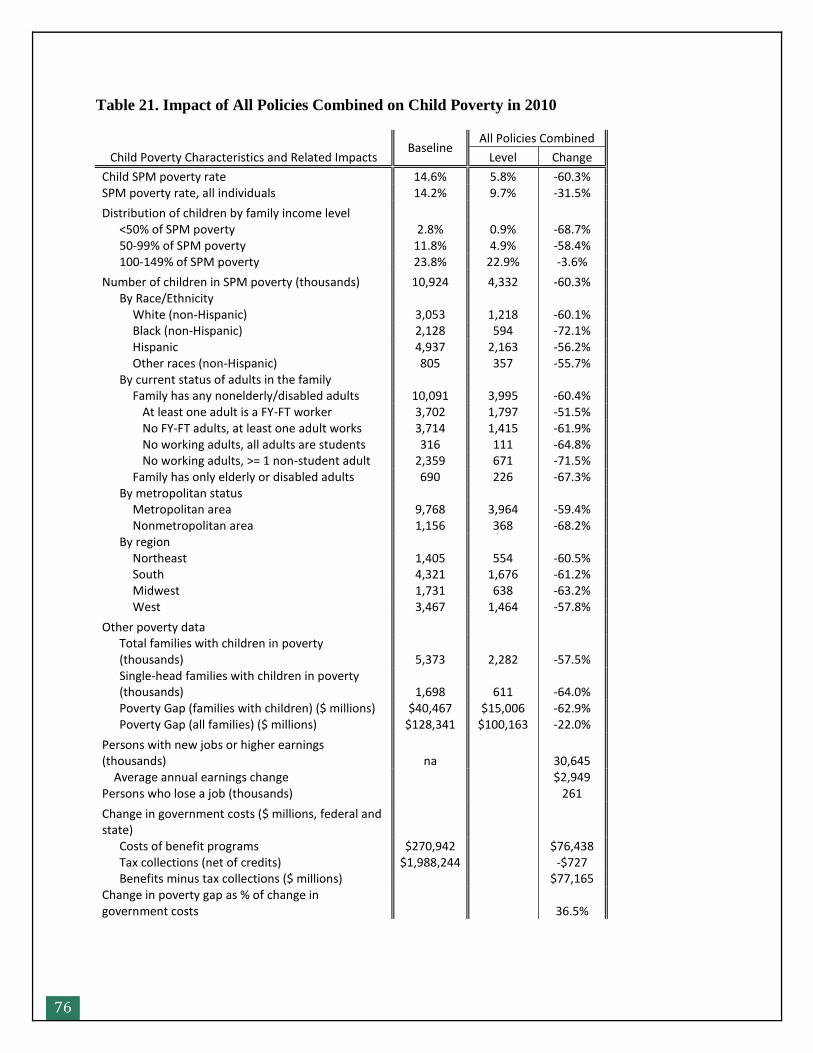
76
Table 21. Impact of All Policies Combined on Child Poverty in 2010
Child Poverty Characteristics and Related Impacts Baseline
All Policies Combined
Level Change
Child SPM poverty rate 14.6% 5.8% -60.3% SPM poverty rate, all individuals 14.2% 9.7% -31.5%
Distribution of children by family income level <50% of SPM poverty 2.8% 0.9% -68.7% 50-99% of SPM poverty 11.8% 4.9% -58.4% 100-149% of SPM poverty 23.8% 22.9% -3.6%
Number of children in SPM poverty (thousands) 10,924 4,332 -60.3% By Race/Ethnicity White (non-Hispanic) 3,053 1,218 -60.1% Black (non-Hispanic) 2,128 594 -72.1% Hispanic 4,937 2,163 -56.2% Other races (non-Hispanic) 805 357 -55.7% By current status of adults in the family Family has any nonelderly/disabled adults 10,091 3,995 -60.4% At least one adult is a FY-FT worker 3,702 1,797 -51.5% No FY-FT adults, at least one adult works 3,714 1,415 -61.9% No working adults, all adults are students 316 111 -64.8% No working adults, >= 1 non-student adult 2,359 671 -71.5% Family has only elderly or disabled adults 690 226 -67.3% By metropolitan status Metropolitan area 9,768 3,964 -59.4% Nonmetropolitan area 1,156 368 -68.2% By region Northeast 1,405 554 -60.5% South 4,321 1,676 -61.2% Midwest 1,731 638 -63.2% West 3,467 1,464 -57.8%
Other poverty data
Total families with children in poverty (thousands) 5,373 2,282 -57.5%
Single-head families with children in poverty (thousands) 1,698 611 -64.0%
Poverty Gap (families with children) ($ millions) $40,467 $15,006 -62.9% Poverty Gap (all families) ($ millions) $128,341 $100,163 -22.0%
Persons with new jobs or higher earnings (thousands) na 30,645
Average annual earnings change $2,949 Persons who lose a job (thousands) 261
Change in government costs ($ millions, federal and state) Costs of benefit programs $270,942 $76,438 Tax collections (net of credits) $1,988,244 -$727 Benefits minus tax collections ($ millions) $77,165 Change in poverty gap as % of change in government costs 36.5%
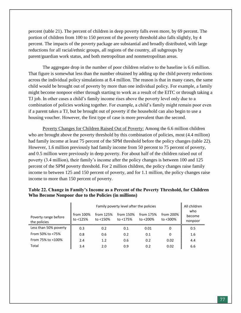
77
percent (table 21). The percent of children in deep poverty falls even more, by 69 percent. The
portion of children from 100 to 150 percent of the poverty threshold also falls slightly, by 4
percent. The impacts of the poverty package are substantial and broadly distributed, with large
reductions for all racial/ethnic groups, all regions of the country, all subgroups by
parent/guardian work status, and both metropolitan and nonmetropolitan areas.
The aggregate drop in the number of poor children relative to the baseline is 6.6 million.
That figure is somewhat less than the number obtained by adding up the child poverty reductions
across the individual policy simulations at 8.4 million. The reason is that in many cases, the same
child would be brought out of poverty by more than one individual policy. For example, a family
might become nonpoor either through starting to work as a result of the EITC or through taking a
TJ job. In other cases a child’s family income rises above the poverty level only due to a
combination of policies working together. For example, a child’s family might remain poor even
if a parent takes a TJ, but be brought out of poverty if the household can also begin to use a
housing voucher. However, the first type of case is more prevalent than the second.
Poverty Changes for Children Raised Out of Poverty: Among the 6.6 million children
who are brought above the poverty threshold by this combination of policies, most (4.4 million)
had family income at least 75 percent of the SPM threshold before the policy changes (table 22).
However, 1.6 million previously had family income from 50 percent to 75 percent of poverty,
and 0.5 million were previously in deep poverty. For about half of the children raised out of
poverty (3.4 million), their family’s income after the policy changes is between 100 and 125
percent of the SPM poverty threshold. For 2 million children, the policy changes raise family
income to between 125 and 150 percent of poverty, and for 1.1 million, the policy changes raise
income to more than 150 percent of poverty.
Table 22. Change in Family’s Income as a Percent of the Poverty Threshold, for Children
Who Become Nonpoor due to the Policies (in millions)
Family poverty level after the policies All children who
become nonpoor
Poverty range before the policies
from 100% to <125%
from 125% to <150%
from 150% to <175%
from 175% to <200%
from 200% to <300%
Less than 50% poverty 0.3 0.2 0.1 0.01 0 0.5
From 50% to <75% 0.8 0.6 0.2 0.1 0 1.6
From 75% to <100% 2.4 1.2 0.6 0.2 0.02 4.4
Total 3.4 2.0 0.9 0.2 0.02 6.6
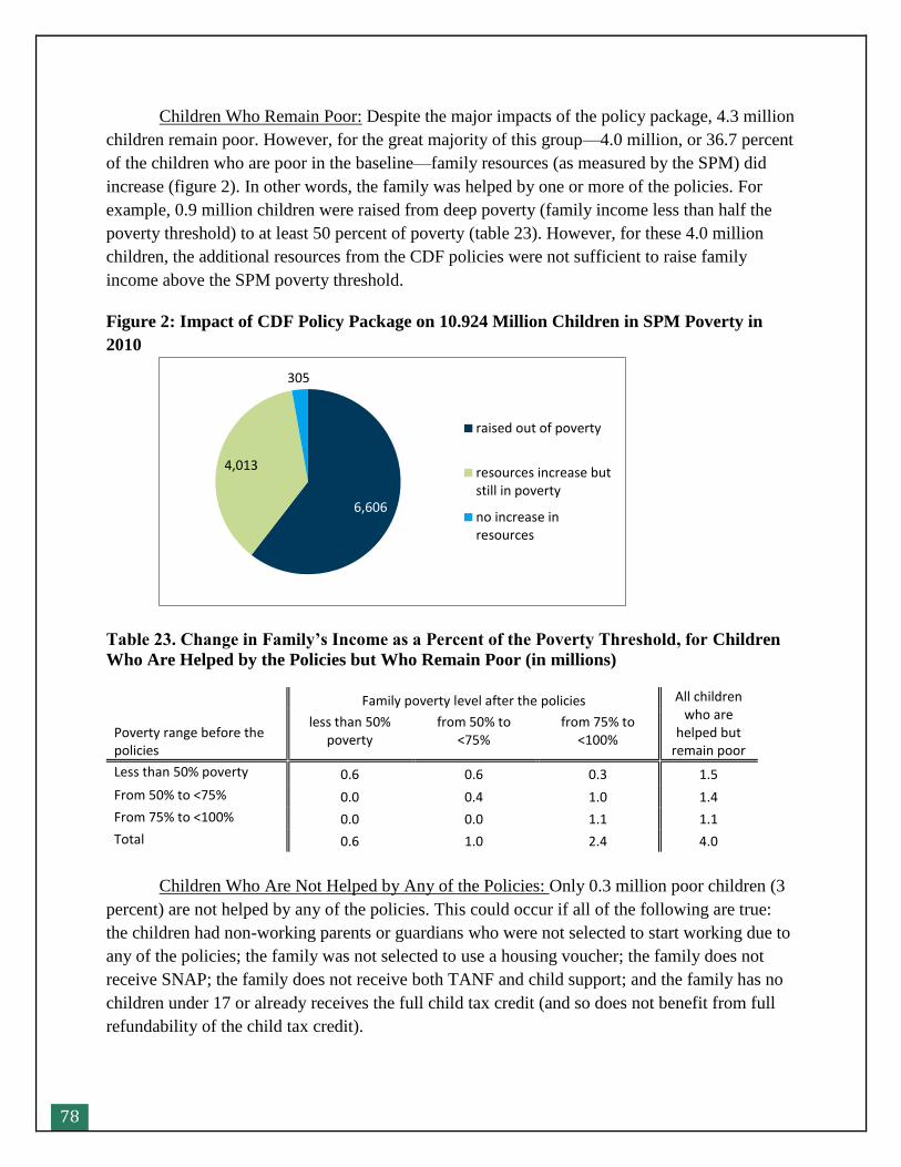
78
Children Who Remain Poor: Despite the major impacts of the policy package, 4.3 million
children remain poor. However, for the great majority of this group—4.0 million, or 36.7 percent
of the children who are poor in the baseline—family resources (as measured by the SPM) did
increase (figure 2). In other words, the family was helped by one or more of the policies. For
example, 0.9 million children were raised from deep poverty (family income less than half the
poverty threshold) to at least 50 percent of poverty (table 23). However, for these 4.0 million
children, the additional resources from the CDF policies were not sufficient to raise family
income above the SPM poverty threshold.
Figure 2: Impact of CDF Policy Package on 10.924 Million Children in SPM Poverty in
2010
Table 23. Change in Family’s Income as a Percent of the Poverty Threshold, for Children
Who Are Helped by the Policies but Who Remain Poor (in millions)
Family poverty level after the policies All children who are
helped but remain poor
Poverty range before the policies
less than 50% poverty
from 50% to <75%
from 75% to <100%
Less than 50% poverty 0.6 0.6 0.3 1.5
From 50% to <75% 0.0 0.4 1.0 1.4
From 75% to <100% 0.0 0.0 1.1 1.1
Total 0.6 1.0 2.4 4.0
Children Who Are Not Helped by Any of the Policies: Only 0.3 million poor children (3
percent) are not helped by any of the policies. This could occur if all of the following are true:
the children had non-working parents or guardians who were not selected to start working due to
any of the policies; the family was not selected to use a housing voucher; the family does not
receive SNAP; the family does not receive both TANF and child support; and the family has no
children under 17 or already receives the full child tax credit (and so does not benefit from full
refundability of the child tax credit).
6,606
4,013
305
raised out of poverty
resources increase butstill in poverty
no increase inresources
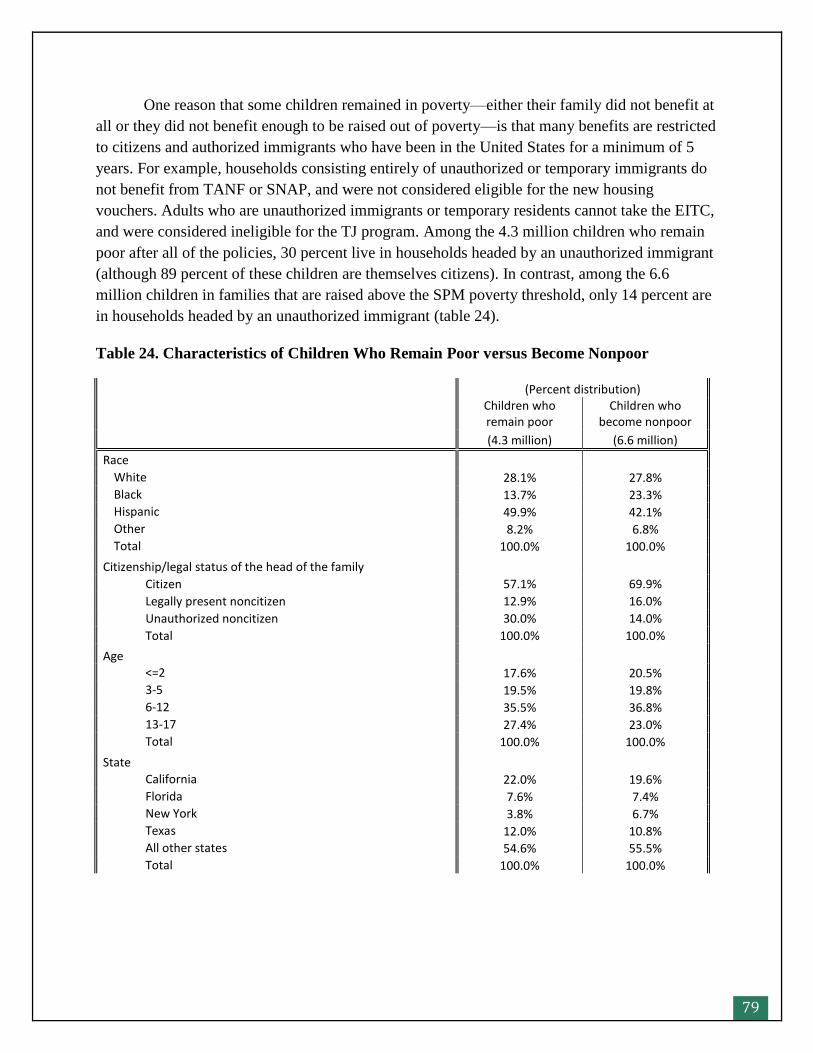
79
One reason that some children remained in poverty—either their family did not benefit at
all or they did not benefit enough to be raised out of poverty—is that many benefits are restricted
to citizens and authorized immigrants who have been in the United States for a minimum of 5
years. For example, households consisting entirely of unauthorized or temporary immigrants do
not benefit from TANF or SNAP, and were not considered eligible for the new housing
vouchers. Adults who are unauthorized immigrants or temporary residents cannot take the EITC,
and were considered ineligible for the TJ program. Among the 4.3 million children who remain
poor after all of the policies, 30 percent live in households headed by an unauthorized immigrant
(although 89 percent of these children are themselves citizens). In contrast, among the 6.6
million children in families that are raised above the SPM poverty threshold, only 14 percent are
in households headed by an unauthorized immigrant (table 24).
Table 24. Characteristics of Children Who Remain Poor versus Become Nonpoor
(Percent distribution) Children who remain poor
Children who become nonpoor
(4.3 million) (6.6 million)
Race
White 28.1% 27.8%
Black 13.7% 23.3%
Hispanic 49.9% 42.1%
Other 8.2% 6.8%
Total 100.0% 100.0%
Citizenship/legal status of the head of the family
Citizen 57.1% 69.9%
Legally present noncitizen 12.9% 16.0%
Unauthorized noncitizen 30.0% 14.0%
Total 100.0% 100.0%
Age
<=2 17.6% 20.5%
3-5 19.5% 19.8%
6-12 35.5% 36.8%
13-17 27.4% 23.0%
Total 100.0% 100.0%
State
California 22.0% 19.6%
Florida 7.6% 7.4%
New York 3.8% 6.7%
Texas 12.0% 10.8%
All other states 54.6% 55.5%
Total 100.0% 100.0%
80
Another group that is overrepresented among those who remained poor is Hispanic
children, who make up 50 percent of all children who remain poor but only 42 percent of
children who are removed from SPM poverty. This is likely related in part to immigrant status,
but also to how often different races/ethnicities participate in benefit programs. As mentioned
above, Hispanic families eligible for SNAP are less likely to receive the benefit than eligible
non-Hispanic families.
Teenagers were less likely than younger children to be raised out of SPM poverty by the
CDF package. Children ages 13 to 17 make up 27 percent of children who remain poor but only
23 percent of children who became nonpoor. One factor is that this age group includes 74,000
children ages 15 through 17 who were considered individually for poverty calculation purposes,
either because they are actually living alone or because they are living with nonrelatives.53 Only
2,000 of these children are raised out of poverty by the policies; they are generally in school and
either not working or working part-time, so they do not benefit from most of the policies.
Another factor is that families with older children tend to have lower rates of participation in
some programs, such as TANF; while the CDF policies do not specifically address TANF, any
existing benefit receipt by the family affects whether or not additional help will allow total
resources to rise above poverty. Also, the Child Tax Credit policy does not benefit families
whose only child is age 17.
There were also some differences in the antipoverty impact by state. Poor children in
metropolitan areas were somewhat less likely to be lifted out of poverty: they make up 91.5
percent of the children who remain poor but 88.0 percent of those raised out of poverty. Among
the largest states, the state showing the strongest impacts from the policies is New York. Of all
the children who remained poor, only 3.8 percent live in New York, while New Yorkers make up
6.7 percent of the children removed from poverty. The state-level differences are likely due to a
combination of factors. One aspect of cross-state variation is program participation rates. For
example, California and Texas both have lower-than-average SNAP participation rates
(Cunnyngham 2014), which would reduce the impact of the policy that raises the SNAP benefit
level. States also vary in the demographic characteristics of their poor populations. One key
difference is that unauthorized immigrants are estimated to comprise a larger share of the
population in California (6.8%) and Texas (6.7%), than in Florida (4.5%) and New York (3.2%)
(Passel and Cohn 2011). Cross-state variations in state income tax policies, safety-net policies,
and the income distribution among lower-income families could all affect the relative impact of
the policy package.
Nonpoor Children Helped by the Policies: In addition to helping poor children, the
package of policies also improved the economic well-being of 32.7 million children who were
53 We follow Census Bureau practices and treat older teens living with nonrelatives as separate from the rest of the
household for poverty purposes. However, if a younger children is unrelated to the rest of the household, we
consider the child as part of the primary family for poverty calculation purposes.
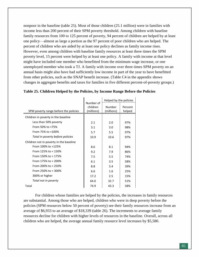
81
nonpoor in the baseline (table 25). Most of those children (25.1 million) were in families with
income less than 200 percent of their SPM poverty threshold. Among children with baseline
family resources from 100 to 125 percent of poverty, 94 percent of children are helped by at least
one policy—almost as large a portion as the 97 percent of poor children who are helped. The
percent of children who are aided by at least one policy declines as family income rises.
However, even among children with baseline family resources at least three times the SPM
poverty level, 15 percent were helped by at least one policy. A family with income at that level
might have included one member who benefitted from the minimum wage increase, or one
unemployed member who took a TJ. A family with income over three times SPM poverty on an
annual basis might also have had sufficiently low income in part of the year to have benefitted
from other policies, such as the SNAP benefit increase. (Table C4 in the appendix shows
changes in aggregate benefits and taxes for families in five different percent-of-poverty groups.)
Table 25. Children Helped by the Policies, by Income Range Before the Policies
SPM poverty range before the policies
Number of children
(millions)
Helped by the policies
Number (millions)
Percent helped
Children in poverty in the baseline
Less than 50% poverty 2.1 2.0 97%
From 50% to <75% 3.1 3.0 98%
From 75% to <100% 5.7 5.5 97%
Total in poverty before policies 10.9 10.6 97%
Children not in poverty in the baseline
From 100% to <125% 8.6 8.1 94%
From 125% to < 150% 9.2 7.9 86%
From 150% to < 175% 7.5 5.5 74%
From 175% to < 200% 6.1 3.5 58%
From 200% to < 250% 8.8 3.4 39%
From 250% to < 300% 6.6 1.6 25%
300% or higher 17.2 2.5 15%
Total not in poverty 64.0 32.7 51%
Total 74.9 43.3 58%
For children whose families are helped by the policies, the increases in family resources
are substantial. Among those who are helped, children who were in deep poverty before the
policies (SPM resources below 50 percent of poverty) see their family resources increase from an
average of $6,933 to an average of $18,339 (table 26). The increments to average family
resources decline for children with higher levels of resources in the baseline. Overall, across all
children who are helped, the average annual family resource level increases by $5,580.
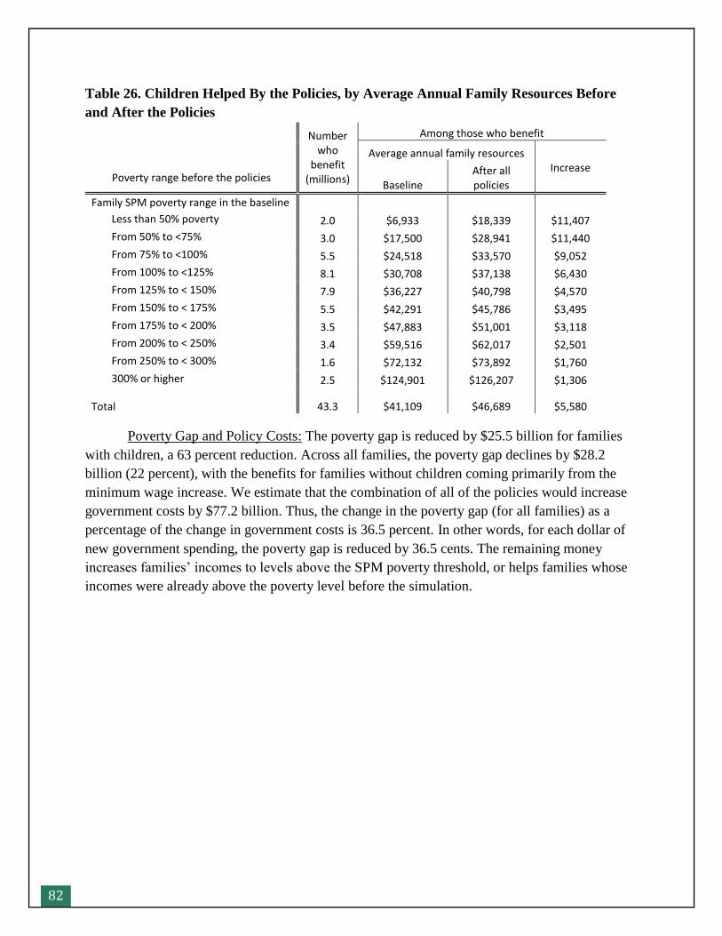
82
Table 26. Children Helped By the Policies, by Average Annual Family Resources Before
and After the Policies
Number who
benefit (millions)
Among those who benefit
Average annual family resources Increase
Poverty range before the policies Baseline
After all policies
Family SPM poverty range in the baseline
Less than 50% poverty 2.0 $6,933 $18,339 $11,407
From 50% to <75% 3.0 $17,500 $28,941 $11,440
From 75% to <100% 5.5 $24,518 $33,570 $9,052
From 100% to <125% 8.1 $30,708 $37,138 $6,430
From 125% to < 150% 7.9 $36,227 $40,798 $4,570
From 150% to < 175% 5.5 $42,291 $45,786 $3,495
From 175% to < 200% 3.5 $47,883 $51,001 $3,118
From 200% to < 250% 3.4 $59,516 $62,017 $2,501
From 250% to < 300% 1.6 $72,132 $73,892 $1,760
300% or higher 2.5 $124,901 $126,207 $1,306
Total 43.3 $41,109 $46,689 $5,580
Poverty Gap and Policy Costs: The poverty gap is reduced by $25.5 billion for families
with children, a 63 percent reduction. Across all families, the poverty gap declines by $28.2
billion (22 percent), with the benefits for families without children coming primarily from the
minimum wage increase. We estimate that the combination of all of the policies would increase
government costs by $77.2 billion. Thus, the change in the poverty gap (for all families) as a
percentage of the change in government costs is 36.5 percent. In other words, for each dollar of
new government spending, the poverty gap is reduced by 36.5 cents. The remaining money
increases families’ incomes to levels above the SPM poverty threshold, or helps families whose
incomes were already above the poverty level before the simulation.
83
Summary and Caveats
The CDF package of policies—including a minimum wage increase, a transitional jobs program,
expanded tax credits, increased availability of housing and child care subsidies, increased
nutrition benefits, and changes to how benefit programs treat families’ child support income—
appears to greatly decrease poverty for US children when poverty is measured with the SPM. Of
the initial number of 10.9 million children in poverty, 6.6 million become nonpoor, a drop of 60
percent. Poverty declines for all racial/ethnic groups, all regions of the country, both
metropolitan and nonmetropolitan areas, and for children living with both working
parents/guardians and non-working parents/guardians. Poverty declines are somewhat less for
children living in a family headed by an unauthorized immigrant, teenagers, and Hispanic
children.
A notable aspect of the policy package is that, even for the children who remain poor,
most of them (4 million) are helped by one or more policies. For instance, 0.9 million children in
deep poverty without the policies remain poor but no longer in deep poverty. Only 0.3 million
poor children are not aided by any of the policies.
Due to income increases for the families of all of the 10.6 million children helped by the
policy, the poverty gap for families with children also fell substantially. That measure—the
aggregate amount of money by which the incomes of poor families with children fall below their
poverty thresholds—fell from $40.5 billion to $15.0 billion, a drop of 63 percent.
Considering the policies individually, the policies with the greatest impact on child
poverty were the increases to in-kind benefits. The increase in housing vouchers had one of the
largest impacts—assuming that new vouchers would be available to any family with children
with income under 150 percent of the poverty guideline that also satisfied a test of rent burden,
and further assuming that 70 percent of those households would be able to use the voucher. That
policy reduced poverty by 21 percent (table 27). New housing vouchers were provided to 2.6
million households, with an average annual subsidy of approximately $9,400. The increase to
SNAP benefits—basing the maximum benefits on the Low-Income Food Plan rather than the
Thrifty Food Plan, for a maximum annual benefit increase of $1,896 for a three-person family—
was the next most effective, reducing child poverty by 16.2 percent. The benefit increase helped
all 10.7 million families with children under 18 currently receiving SNAP in the average month
of the year; the number of average monthly participating families would increase by 1.3 million
due to the benefit increase.
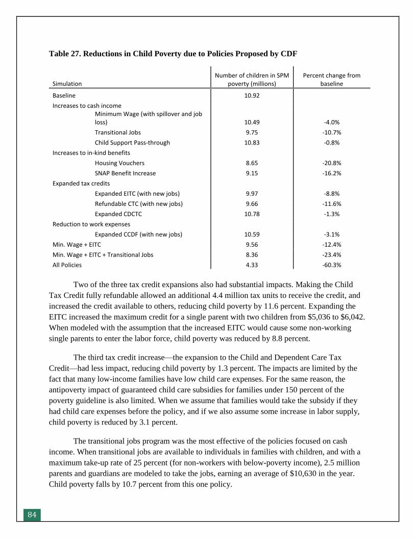
84
Table 27. Reductions in Child Poverty due to Policies Proposed by CDF
Simulation Number of children in SPM
poverty (millions) Percent change from
baseline
Baseline 10.92
Increases to cash income
Minimum Wage (with spillover and job loss) 10.49 -4.0%
Transitional Jobs 9.75 -10.7%
Child Support Pass-through 10.83 -0.8%
Increases to in-kind benefits
Housing Vouchers 8.65 -20.8%
SNAP Benefit Increase 9.15 -16.2%
Expanded tax credits
Expanded EITC (with new jobs) 9.97 -8.8%
Refundable CTC (with new jobs) 9.66 -11.6%
Expanded CDCTC 10.78 -1.3%
Reduction to work expenses
Expanded CCDF (with new jobs) 10.59 -3.1%
Min. Wage + EITC 9.56 -12.4%
Min. Wage + EITC + Transitional Jobs 8.36 -23.4%
All Policies 4.33 -60.3%
Two of the three tax credit expansions also had substantial impacts. Making the Child
Tax Credit fully refundable allowed an additional 4.4 million tax units to receive the credit, and
increased the credit available to others, reducing child poverty by 11.6 percent. Expanding the
EITC increased the maximum credit for a single parent with two children from $5,036 to $6,042.
When modeled with the assumption that the increased EITC would cause some non-working
single parents to enter the labor force, child poverty was reduced by 8.8 percent.
The third tax credit increase—the expansion to the Child and Dependent Care Tax
Credit—had less impact, reducing child poverty by 1.3 percent. The impacts are limited by the
fact that many low-income families have low child care expenses. For the same reason, the
antipoverty impact of guaranteed child care subsidies for families under 150 percent of the
poverty guideline is also limited. When we assume that families would take the subsidy if they
had child care expenses before the policy, and if we also assume some increase in labor supply,
child poverty is reduced by 3.1 percent.
The transitional jobs program was the most effective of the policies focused on cash
income. When transitional jobs are available to individuals in families with children, and with a
maximum take-up rate of 25 percent (for non-workers with below-poverty income), 2.5 million
parents and guardians are modeled to take the jobs, earning an average of $10,630 in the year.
Child poverty falls by 10.7 percent from this one policy.
85
The full pass-through and disregard of child support income for TANF recipients,
combined with a $100-per-child child support disregard in the SNAP program, reduces child
poverty by 0.8 percent. The impact of this policy is muted by the fact that relatively few families
receive TANF, and only a minority of those families have child support paid on their behalf. The
modeled policy reflects pass-through and disregard of currently due child support only. Passing
through all collections of past-due child support (arrears) would have additional antipoverty
effects.
Finally, the proposed increase to the minimum wage—$10.10 for most workers and
$7.07 for tipped workers—reduces child poverty by 4 percent when we assume that there would
also be wage increases for workers earning slightly below the current minimum or slightly above
the new minimum, as well as a small amount of job loss. The impacts of the minimum wage are
minimized by the fact that four-fifths of the affected workers live in families that are not poor by
the SPM definition. Among those minimum wage workers who do live in poor families, many do
not work full-year full-time, and increases in earnings may be offset by reductions in benefits.
We estimate that the combination of all of the policies would increase government costs
by $77.2 billion. Considering eight different benefit programs—unemployment compensation,
SSI, TANF, housing subsidies, SNAP, LIHEAP, WIC, and CCDF subsidies—estimated costs
increase by $40.3 billion, or 14.9 percent. (Possible increases in administrative costs due to
benefit expansions are not estimated.) Considering payroll taxes and federal and state income
taxes, tax collections fall by an estimated $0.7 billion, due to a combination of increased tax
credits offset by increases in tax liability from new earnings. The transitional jobs program is
estimated to cost $36.2 billion, not including administrative costs. In relative terms, the estimated
cost of the entire package equals 0.5 percent of the size of United States Gross National Product
in 2010 ($15.0 trillion), 11 percent of the aggregate 2010 benefits paid in Social Security
retirement and disability benefits, or about 16 percent higher than the 2010 cost of SNAP
benefits.54
The change in the poverty gap—a total reduction of $28.2 billion across all poor
families—is 36.5 percent of the total estimated cost of the package. In other words, for each
dollar of new government spending, the poverty gap for families with children is reduced by 36.5
cents. The remaining money increases families’ incomes to levels above the SPM poverty
threshold, or helps families whose incomes were already above the poverty level before the
simulation.
Several caveats are important to note in considering the results of the analysis.
Considering the modeling of the individual policies, much of the analysis is based on applying
54 Aggregate Social Security retirement, survivors, and disability benefit payments were $701.6 billion in 2010
according to the Social Security Bulletin’s Annual Statistical Supplement, tables 4.A1 and 4.A2. SNAP benefit
payments in calendar year 2010 amounted to $66.6 billion.
86
specific tax and benefit rules, but the modeling of employment effects—spillover effects and job
loss from a minimum wage increase, and increased labor supply from enhanced tax credits or
subsidies—involves uncertainty. For example, if we have underestimated (or overestimated) the
extent of job loss from a minimum wage increase, we could be overestimating (or
underestimating) the antipoverty impacts of the policy. Another limitation regarding our
minimum wage analysis is that we do not capture any broader economic impacts that could
either help or hurt lower-income families. For example, higher incomes in a low-income
neighborhood might generate more economic activity and more opportunities; however, it is also
possible that businesses might raise prices and low-income families would see their expenses
rise. Turning to our analysis of an EITC expansion, our estimates likely understate the costs and
antipoverty effects because we do not model noncompliance with EITC rules and data
limitations also contribute to an overall shortfall in simulated EITC.
Three broad caveats apply to the analysis as a whole. First, the analysis is based on data
representing the population, economy, and policies in 2010; the relative impacts of policies
would be different today. For example, since the unemployment rate is somewhat lower today
than in 2010, the number of people taking advantage of a TJ program might be somewhat lower.
However, whether the antipoverty impact of a policy (in percentage terms) would be higher or
lower today would depend on many factors, including the number of affected families in poverty
and the distribution of their incomes relative to the poverty thresholds. Second, we do not
incorporate into the model how the new programs would be paid for. If new policies were funded
by reducing spending on some current programs or by altering the tax system, the resources of
low-income families could be impacted by those changes as well as by the new antipoverty
policies. Third, the model focuses on capturing interconnections among benefit and tax
programs, but does not capture broader behavioral and economic connections. For example, in
modeling the change to the child support pass-through policy, we do not capture the fact that
noncustodial parents would likely pay more child support if they knew that more money was
reaching their children; thus, we are probably underestimating the antipoverty impact of that
policy. Further, reductions in poverty for today’s children could have benefits on their education,
health, and employment as young adults and as parents, with the potential to reduce poverty for
the generation of children.
Focusing on the near term, the analysis shows that the CDF package of policy changes
could reduce child poverty by approximately 60 percent, and could increase family resources for
almost all poor children. The cost is equivalent to 0.5 percent of GDP. As one measure of the
effectiveness of the spending, the change in the poverty gap equals 36.5 percent of the estimated
cost. Further research could consider the implications of varying the assumptions about
employment effects, consider the distributional impacts of different approaches to paying for
these types of programs, and assess the potential longer-run impacts.
87
References
Allegretto, Sylvia A., and Kai Filion. 2011. “Waiting for Change: The $2.13 Federal
Subminimum Wage.” Economic Policy Institute.
Averett, Susan, H. Elizabeth Peters, and Donald Waldman. 1997. “Tax Credits, Labor Supply,
and Child Care.” Review of Economics and Statistics 79 (1).
Blau, David. 2003. “Child Care Subsidy Programs.” In Means-Tested Transfer Programs in the
United States, Robert A. Moffitt, ed. Chicago: University of Chicago Press.
http://www.nber.org/chapters/c10260
Citro, Constance F., and Robert T. Michael, eds. 1995. Measuring Poverty: A New Approach.
Washington, D.C.: National Academy Press.
Community Advocates Public Policy Institute. 2012. “Poverty in Wisconsin Can Be
Dramatically Reduced.” http://communityadvocates.net/userimages/PathwaysResult.pdf
Congressional Budget Office. 2014a. “The Budget and Economic Outlook: 2014 to 2024.”
Washington, D.C. http://www.cbo.gov/publication/45010
Congressional Budget Office. 2014b. “The Effects of a Minimum Wage Increase on
Employment and Family Income.” Washington, D.C.
Cooper, David and Doug Hall. 2013. “Raising the Federal Minimum Wage to $10.10 Would
Give Working Families, and the Overall Economy, a Much-Needed Boost.” Economic
Policy Institute, Briefing Paper 357. http://www.epi.org/publication/bp357-federal-
minimum-wage-increase/
Crandall-Hollick, Margot. 2013. “The Child Tax Credit: Current Law and Legislative History.”
Congressional Research Service Report R41873.
http://www.law.umaryland.edu/marshall/crsreports/crsdocuments/R41873_03252013.pdf
Cunnyngham, Karen. “Reaching Those in Need: State Supplemental Nutrition Assistance
Program Participation Rates in 2011.” 2014. USDA Food and Nutrition Service, Report
Summary.
Doolittle, Fred, Steve Bell, Howard Bloom, George Cave, James Kemple, Larry Orr, Linda
Traeger and John Wallace. 1993. “A Summary of the Design and Implementation of the
National JTPA Study.” MDRC.
http://www.upjohninst.org/sites/default/files/erdc/reports/njtpareport.pdf
88
Eissa, Nada, and Hilary Hoynes. 2006. “Behavioral Responses to Taxes: Lessons from the EITC
and Labor Supply.” In Tax Policy and the Economy, Vol. 20, James Poterba, ed., MIT
Press.
Eslami, Esa, and Karen Cunnyngham. 2014. “Supplemental Nutrition Assistance Program
Participation Rates: Fiscal Years 2010 and 2011.” USDA FNS, Current Perspectives on
SNAP Participation series.
Finkel, Meryl and Larry Buron. 2001. “Study on Section 8 Voucher Success Rates: Volume I
Quantitative Study of Success Rates in Metropolitan Areas.” Washington, D.C.: US
Department of Housing and Urban Development, Office of Policy Development and
Research.
Fox, Liana, Irv Garfinkel, Neeraj Kaushal, Jane Waldfogel, and Christopher Wimer. 2014.
“Waging War on Poverty: Historical Trends in Poverty Using the Supplemental Poverty
Measure.” National Bureau of Economic Research Working Paper No. 19789.
Garner, Thesia I. 2010. “Supplemental Poverty Measure Thresholds: Laying the Foundation.”
Washington, D.C.: US Department of Labor, Bureau of Labor Statistics.
Giannarelli, Linda, Joyce Morton, and Laura Wheaton. 2007. “Estimating the Antipoverty
Effects of Changes in Taxes and Benefits with the TRIM3 Microsimulation Model.”
Washington, D.C.: The Urban Institute.
http://www.urban.org/UploadedPDF/411450_Estimating_Effects.pdf.
Giannarelli, Linda, Kye Lippold, and Michael Martinez-Schiferl. 2012. “Reducing Poverty in
Wisconsin: Analysis of the Community Advocates Public Policy Institute Policy
Package.” Washington, D.C.: The Urban Institute.
http://www.urban.org/publications/412604.html
Grogger, Jeffrey. 2003. “The Effects of Time Limits, the EITC, and Other Policy Changes on
Welfare Use, Work, and Income among Female-Headed Families.” The Review of
Economics and Statistics 85(2): 394-408.
Fitzpatrick, Maria. 2012. “Revising Our Thinking About the Relationship Between Maternal
Labor Supply and Preschool.” Journal of Human Resources 20(47):583-612.
http://jhr.uwpress.org/content/47/3/583.abstract
Hartline-Grafton, Heather and James Weill. 2012. “Replacing the Thrifty Food Plan in Order to
Provide Adequate Allotments for SNAP Beneficiaries.” Washington, D.C.: Food
Research and Action Center.
Herbst, Chris. 2010. “The Labor Supply Effects of Child Care Costs and Wages in the Presence
of Subsidies and the Earned Income Tax Credit.” Review of Economics of the Household
8:199-230.
89
Internal Revenue Service. 2014. "Compliance Estimates for the Earned Income Tax Credit
Claimed on 2006-2008 Returns." Publication 5162 (8-2014) Catalog Number 66766H.
Washington, D.C.: Department of the Treasury Internal Revenue Service.
Kassabian, David, Tracy Vericker, David Searle, and Mary Murphy. 2011. “Welfare Rules
Databook: State TANF Policies as of July 2010.” Urban Institute report to HHS/ACF.
Laughlin, Lynda. 2013. “Who’s Minding the Kids? Child Care Arrangements, Spring 2011”.
Census Bureau, Household Economic Studies, P70-135.
Lippold, Kye, Austin Nichols, and Elaine Sorensen. 2010. “Evaluation of the $150 Child Support
Pass-Through and Disregard Policy in the District of Columbia.” Project report,
http://www.urban.org/publications/412779.html.
Michalopoulos, Charles. 2010. “Effects of Reducing Child Care Subsidy Copayments in
Washington State.” OPRE 2011-2. Washington, D.C.: Office of Planning, Research and
Evaluation, Administration for Children and Families, US Department of Health and
Human Services. http://www.mdrc.org/publication/effects-reducing-child-care-subsidy-
copayments-washington-state
Michalopoulos, Charles, Erika Lundquist, and Nina Castells. 2010. “The Effects of Child Care
Subsidies for Moderate-Income Families in Cook County, Illinois.” OPRE 2011-3.
Washington, D.C.: Office of Planning, Research and Evaluation, Administration for
Children and Families, US Department of Health and Human Services.
http://www.mdrc.org/publication/effects-child-care-subsidies-moderate-income-families-
cook-county-illinois
Miller, Benjamin, and Kevin Mumford. 2011. "Personal Income Tax Salience: Evidence from
the Child and Dependent Care Credit Expansion." Purdue University Economics
Working Papers 1261, Purdue University, Department of Economics.
Mills, Gregory, Daniel Gubits, Larry Orr, David Long, Judie Feins, Bulbul Kaul, Michelle
Wood, Amy Jones & Associates, Cloudburst Consulting, and the QED Group. 2006.
“Effects of Housing Vouchers on Welfare Families.” 2006. Project report from Abt
Associates to the US Department of Housing and Urban Development.
Mirengoff, William, Lester Rindler, Harry Greenspan, Scott Seablom, and Lois Black. 1980. The
New CETA: Effect on Public Service Employment Programs: Final Report. National
Research Council.
http://books.google.com/books?id=bjUrAAAAYAAJ&lpg=PA24&ots=Ut8XxgKL4H&d
q=The%20New%20CETA&pg=PA46#v=onepage&q&f=false
Nichols, Austin, Elaine Sorensen, and Kye Lippold. 2012. “The New York Noncustodial Parent
EITC: Its Impact on Child Support Payments and Employment.” Urban Institute project
report.
90
Neumark, David, and William Wascher. 2006. “Minimum Wages and Employment: A Review
of Evidence from the New Minimum Wage Research.” NBER Working Paper 12663.
Cambridge: National Bureau of Economic Research.
Passel, Jeffrey S., and D’Vera Cohn. 2011. “Unauthorized Immigrant Population: National and
State Trends 2010”. Pew Research Hispanic Trends Project.
Passel, Jeffrey S., Jennifer Van Hook, and Frank D. Bean. 2006. Narrative Profile with
Adjoining Tables of Unauthorized Migrants and Other Immigrants, Based on Census
2000: Characteristics and Methods. Warrington, PA: Sabre Systems, Inc.
Pavetti, LaDonna, Liz Schott, and Elizabeth Lower-Basch. 2011. “Creating Subsidized
Employment Opportunities for Low-Income Parents: The Legacy of the TANF
Emergency Fund.” Center on Budget and Policy Priorities and CLASP.
http://www.cbpp.org/files/2-16-11tanf.pdf
Schmitt, John. 2013. “Why Does the Minimum Wage Have No Discernible Impact on
Employment?” Washington D.C.: Center for Economic Policy Research.
Short, Kathleen S. 2011. “The Research Supplemental Poverty Measure: 2010.” Washington,
D.C.: US Census Bureau.
——— 2013. “The Research Supplemental Poverty Measure: 2012.” Washington, D.C.: US
Census Bureau.
Short, Kathleen S. and Thesia I. Garner. 2012. “The Supplemental Poverty Measure: A Joint
Project between the Census Bureau and the Bureau of Labor Statistics. Washington,
D.C.: US Census Bureau and US Department of Labor, Bureau of Labor Statistics.
Tekin, Erdal. 2007. “Childcare Subsidies, Wages, and Employment of Single Mothers.” Journal
of Human Resources 42(2):453-487. http://www.jstor.org/stable/40057313
Treasure Inspector General for Tax Administration (TIGTA). 2014. "The Internal Revenue
Service Fiscal Year 2013 Improper Payment Reporting Continues to Not Comply with
the Improper Payments Elimination and Recovery Act. Reference Number: 2014-40-027.
Washington, D.C.: US Department of Treasury.
US Census Bureau. 2010. Observations from the Interagency Technical Working Group on
Developing a Supplemental Poverty Measure. Washington, D.C.: US Census Bureau.
http://www.census.gov/hhes/www/poverty/SPM_TWGOobservations.pdf.
——— 2011a. “Current Population Survey, 2011 Annual Social and Economic (ASEC)
Supplement.” Available on the Census Bureau’s website at
http://www.census.gov/prod/techdoc/cps/cpsmar11.pdf.
——— 2011b. “Income, Poverty, and Health Insurance Coverage in the United States: 2010.”
Press release, September 13, 2011.
91
US Department of Housing and Urban Development. 2013. “Worst Case Housing Needs 2011:
Report to Congress”. February 2013.
Wolkwitz, Kari. Detailed Tables of Food Stamp Program Participation Rates: 2000 to 2005.
Food and Nutrition Service, Office of Research and Analysis, US Department of
Agriculture. Alexandria, VA, 2008.
Ziliak, James, Charles Hokayem, and Bradley Hardy. 2008. “Child Care Subsidies and the
Economic Well-Being of Recipient Families: A Survey and Implications for Kentucky.”
University of Kentucky Center for Poverty Research.
http://www.ukcpr.org/Publications/ChildCareSubsidies.pdf
92
Appendix A. Validation of TRIM3 Baseline
Simulations
The starting point for this analysis is a version of the CY 2010 CPS-ASEC data that was
previously augmented by Urban Institute staff to create a richer view of families’ resources and
program participation under actual 2010 policies.55 For each of the households in the CPS-ASEC
data, TRIM was used to simulate the major benefit and tax programs, creating new items of
information for each household telling if they are eligible for various programs, their level of tax
liability, and so on. In modeling benefit programs, TRIM3 selects a caseload among program-
eligible families such that the simulated caseload comes close to the actual caseload in terms of
size and key characteristics. The simulation of tax liability does not generally involve a selection
process, since individuals are all assumed to pay all taxes that they owe.56
For both benefit and tax simulations, we compare the simulation results to administrative
data to validate the results. The results of that validation are shown in table A1. In brief, the table
shows the following:
SSI: SSI income is reported in the CPS-ASEC, but the aggregate amount reported ($39.7
billion) falls substantially below the actual paid to noninstitutionalized individuals ($48.7
billion). TRIM3’s simulation assigns additional benefits to come within 1.3 percent of the
actual figure. The simulated caseload is very close to the actual caseload for both adults and
children receiving SSI.
TANF: TANF income is also reported in the CPS-ASEC, but the aggregate amount reported
($5.4 billion) falls substantially below the actual amount ($9.0 billion). TRIM3’s simulation
assigns additional families and benefits to come within a few percent of the actual figures.
SNAP: Like SSI and TANF, SNAP benefits are underreported in the CPS-ASEC data.
TRIM3’s simulation of SNAP results in a caseload and benefit levels very close to the
administrative data figures.
Public and subsidized housing: Households report in the CPS-ASEC if they live in public or
subsidized housing. After excluding apparently ineligible households, the resulting number is
close to the administrative caseload target. The model also estimates the value of living in
public or subsidized housing.
55 A set of 2010 baseline simulations was previously created under contract with HHS/ASPE. The simulations for
this analysis are slightly modified, incorporating recent enhancements to methods.
56 There is one exception. The number of tax units apparently eligible for the federal Child and Dependent Care
Credit exceeds the number who take the credit, so a subset is probabilistically selected.

93
LIHEAP: LIHEAP receipt is substantially underreported in the CPS-ASEC data. TRIM3
identifies a caseload that is very close to the actual figure, and also assigns a benefit value.
WIC: As with the other programs, WIC enrollment is underreported in the CPS-ASEC data.
TRIM3 identifies a caseload of infants and children that is very close to the actual figure; the
assignment of women who receive WIC falls short of the actual figure because the survey
data do not identify pregnancy.
CCDF child care subsidies: The CPS-ASEC data does not include any information on
CCDF-funded child care subsidies. The model identifies subsidy-eligible families and selects
a caseload that comes very close to actual figures by key characteristics. The survey-reported
information on amount of out-of-pocket child care expenses is also used to guide the
selection of the caseload; for example, families that reported child care expenses are not
selected as subsidized if they would owe no copayment in their state. The model also
simulates the value of the subsidy, producing an aggregate value within 10 percent of the
actual figure.
Payroll taxes: Payroll taxes are not reported in the CPS-ASEC. The model’s simulated
payroll tax amount is within 2 percent of the actual.
Federal income taxes: Federal income taxes and credits are not reported in the survey data.
TRIM3 applies the federal income tax rules in as much detail as feasible given the survey
data. We do not show a comparison to actual figures since our simulation for this project
deviated from actual 2010 policies by excluding the Making Work Pay credit. Focusing on
the EITC, TRIM3 finds 26 percent fewer tax units eligible for the EITC than actually took
the credit in 2010. This is likely due to a combination of factors, including the fact that
TRIM3 models full compliance with all rules, and differences between how families describe
their circumstances in survey data versus for tax purposes.
State income taxes: State income tax liabilities are not reported in the survey data. TRIM3
simulates these taxes, using the detailed rules of each state that has an income tax system.
The aggregate amount of state income taxes simulated across all states is almost exactly
equal to the actual figure.
Detailed documentation on TRIM3 simulation methods for each tax and benefit program
is available on the project’s website, http://trim.urban.org. The documentation includes
discussion of procedures as well as the specific rules that were applied in modeling each
program.
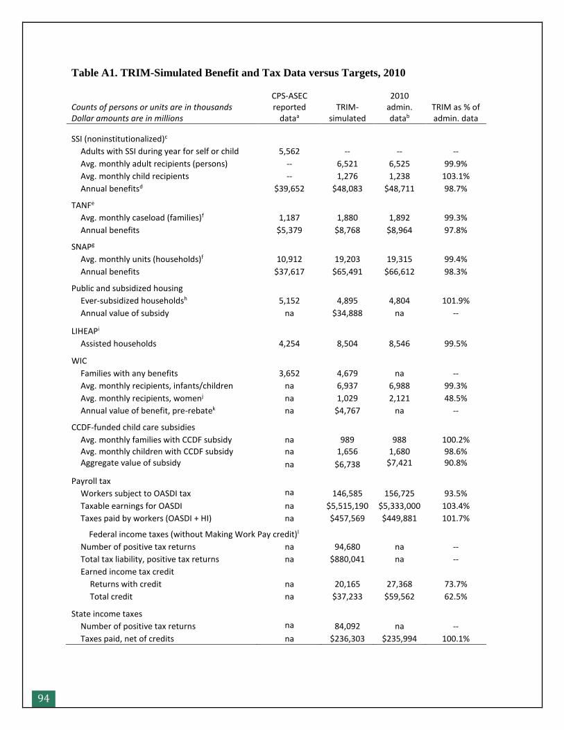
94
Table A1. TRIM-Simulated Benefit and Tax Data versus Targets, 2010
Counts of persons or units are in thousands Dollar amounts are in millions
CPS-ASEC reported
dataa TRIM-
simulated
2010 admin. datab
TRIM as % of admin. data
SSI (noninstitutionalized)c Adults with SSI during year for self or child 5,562 -- -- --
Avg. monthly adult recipients (persons) -- 6,521 6,525 99.9%
Avg. monthly child recipients -- 1,276 1,238 103.1%
Annual benefitsd $39,652 $48,083 $48,711 98.7%
TANFe Avg. monthly caseload (families)f 1,187 1,880 1,892 99.3%
Annual benefits $5,379 $8,768 $8,964 97.8%
SNAPg Avg. monthly units (households)f 10,912 19,203 19,315 99.4%
Annual benefits $37,617 $65,491 $66,612 98.3%
Public and subsidized housing Ever-subsidized householdsh 5,152 4,895 4,804 101.9%
Annual value of subsidy na $34,888 na --
LIHEAPi Assisted households 4,254 8,504 8,546 99.5%
WIC Families with any benefits 3,652 4,679 na --
Avg. monthly recipients, infants/children na 6,937 6,988 99.3%
Avg. monthly recipients, womenj na 1,029 2,121 48.5%
Annual value of benefit, pre-rebatek na $4,767 na -- CCDF-funded child care subsidies
Avg. monthly families with CCDF subsidy na 989 988 100.2%
Avg. monthly children with CCDF subsidy na 1,656 1,680 98.6% Aggregate value of subsidy na $6,738 $7,421 90.8%
Payroll tax Workers subject to OASDI tax na 146,585 156,725 93.5%
Taxable earnings for OASDI na $5,515,190 $5,333,000 103.4%
Taxes paid by workers (OASDI + HI) na $457,569 $449,881 101.7%
Federal income taxes (without Making Work Pay credit)l Number of positive tax returns na 94,680 na --
Total tax liability, positive tax returns na $880,041 na --
Earned income tax credit Returns with credit na 20,165 27,368 73.7%
Total credit na $37,233 $59,562 62.5%
State income taxes Number of positive tax returns na 84,092 na --
Taxes paid, net of credits na $236,303 $235,994 100.1%
95
na = not available; avg. = average; admin. = administrative Notes to Table A1 a. CPS-ASEC reported data included the data that are "allocated" by the Census Bureau in cases of nonresponse. Items not asked in the survey that are imputed by the Census Bureau (such as tax liabilities) are not shown. b. Administrative figures are adjusted or combined for consistency with simulation concepts. In particular, fiscal year administrative data are adjusted for greater comparability with calendar year simulated data, and benefits paid to individuals in the territories are excluded. Benefits include both federally and state-funded amounts. c. SSI figures include state supplements. d. Administrative data for SSI include retroactive payments, which are approximately 9 percent of total payments; TRIM does not simulate retroactive payments. e. Includes benefits funded by federal TANF money and separate state programs, but not solely state-funded programs. The administrative figure for aggregate benefits is computed as the average per unit benefit from administrative microdata applied to the actual caseload. f. For TANF and SNAP, an average monthly caseload is computed using the CPS-reported number of months that benefits are received. g. The administrative figures for SNAP exclude SNAP disaster assistance. h. Administrative figure is the number of occupied public and assisted units. i. An exact unduplicated number of assisted households is not available; an unduplicated count is estimated using estimates of the overlap between groups receiving heating, cooling, and crisis benefits. j. Benefits to pregnant women are not captured in the TRIM simulation. k. The TRIM benefit amount includes the pre-rebate value of infant formula. An administrative figure for WIC food costs net of the rebate was not available. l. The Making Work Pay credit—a refundable credit of $400 for individual tax units and $800 for married couples in tax years 2009 and 2010—was excluded from this analysis. TRIM3's simulation of 2010 federal tax policy including the MWP credit was within 4 percent of target for number of positive-tax returns and fell 10 percent short of target for total income tax liability.
96
Appendix B. Effects of Selected Stimulus
Provisions on Child Poverty
In addition to simulating the effects of the policy package on child poverty, the Children’s
Defense Fund requested that the Urban Institute simulate the effects of eliminating some of the
stimulus provisions enacted in the American Recovery and Reinvestment Act of 2009 (ARRA)
on child poverty. These provisions were:
An increase of roughly 14 percent in the amount of SNAP benefits. This provision of ARRA
expired in November 2013.
Several provisions related to tax credits, which were considered together. All of these
provisions were extended by the American Taxpayer Relief Act of 2012, and are currently
scheduled to expire in 2017.
o A $2,010 increase in the length of the EITC plateau region for taxpayers married
filing jointly (intended to mitigate marriage penalties).
o An expansion of the EITC to provide greater benefits for families with three
children; the credit parameters for such families were the same as for families
with two children, but the credit phased in at a rate of 45 percent of earned
income rather than 40 percent.
o The expansion of the Additional Child Tax Credit to provide benefits phasing in
at 15 percent of earned income above $3,000 (rather than the scheduled 2010
income threshold of $12,550).57
Our simulation excluding these provisions thus indicates the degree to which child
poverty would have been higher in 2010 if these ARRA provisions had not been enacted or had
already expired at that time.
Methods: We simulated the removal of these ARRA provisions by adjusting parameters
in TRIM related to the SNAP program and federal taxes. We simulated first the removal of the
SNAP provisions only, and then the removal of both the SNAP and tax provisions.
57 While the Additional Child Tax Credit already had a slightly lowered refundability threshold before ARRA due to
2008 stimulus legislation, we assumed that 2008 legislation would have expired, so that the refundability threshold
would have returned to its current law level of $12,550 (the same as the 2009 level, given that there was no inflation
of tax parameters from 2009 to 2010). See Crandall-Hollick (2013) for more discussion of this issue.
97
We used unpublished data from the US Department of Agriculture Food and Nutrition
Service to estimate the levels of SNAP allotments that would have applied without the ARRA
expansion. For the tax credits, we adjusted the parameters of the EITC and Additional Child Tax
Credit to conform to the levels that would have applied without the ARRA legislation, as
indicated by published figures from the Congressional Research Service (Crandall-Hollick 2013)
and the Tax Policy Center.
Results: The ARRA policies had fairly substantial effects on child poverty, as shown in
table B1. Removing the expanded SNAP benefit levels alone (as actually occurred in November
2013) would have increased child SPM poverty in 2010 by 7.6 percent, to a poverty rate of 15.7
percent. Removing the tax provisions in addition to reducing SNAP benefits would have
increased child poverty by an additional 6.6 percent (a 14.2 percent increase relative to baseline),
leading to a poverty rate of 16.7 percent. The expirations would have led to an increase of 17
percent in the number of children in deep poverty, and a 15 percent increase in the child poverty
gap.
Focusing on the SNAP benefit decrease, the percentage increase in poverty was greater
for white children (9.7 percent) and black children (10.5 percent) versus Hispanic children (5.2
percent), which is likely related to the lower SNAP participation rate for Hispanic families
(Wolkwitz 2008). Children in nonmetropolitan areas were also more strongly affected, with 14.1
percent more in poverty without the SNAP benefit increase (compared to a 7 percent increase in
metropolitan areas). Children living in the Midwest had a larger increase in poverty with the
SNAP decrease, with 12 percent more children in poverty compared to 4 to 9 percent in other
regions. Overall, while the government would have spent $12.5 billion fewer dollars on SNAP
benefits, this money was relatively well targeted in reducing poverty, with 45 cents of every
dollar reducing the SPM poverty gap.
Considering the removal of both the tax and SNAP stimulus provisions, white children
would have seen an 18.1 percent increase in poverty, and black children a 16.2 percent increase,
versus an 11.1 percent increase for Hispanic children. Poverty would also have substantially
increased, by 17 to 18 percent, for families with at least one adult who was working (since the
tax provisions solely benefitted working families). Overall, the government would have spent
$21.8 billion dollars fewer on SNAP benefits and tax credits combined, but 37 percent of that
spending was serving to reduce the SPM poverty gap.
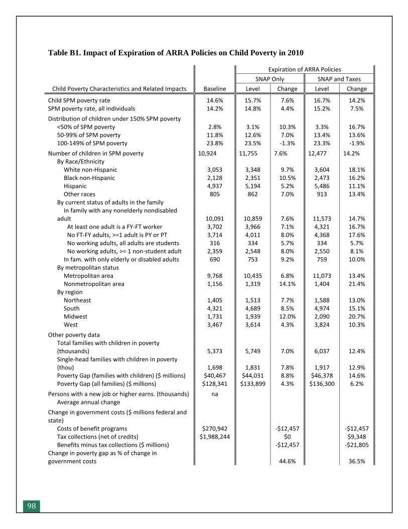
98
Table B1. Impact of Expiration of ARRA Policies on Child Poverty in 2010
Child Poverty Characteristics and Related Impacts Baseline
Expiration of ARRA Policies
SNAP Only SNAP and Taxes
Level Change Level Change
Child SPM poverty rate 14.6% 15.7% 7.6% 16.7% 14.2% SPM poverty rate, all individuals 14.2% 14.8% 4.4% 15.2% 7.5%
Distribution of children under 150% SPM poverty <50% of SPM poverty 2.8% 3.1% 10.3% 3.3% 16.7% 50-99% of SPM poverty 11.8% 12.6% 7.0% 13.4% 13.6% 100-149% of SPM poverty 23.8% 23.5% -1.3% 23.3% -1.9%
Number of children in SPM poverty 10,924 11,755 7.6% 12,477 14.2% By Race/Ethnicity White non-Hispanic 3,053 3,348 9.7% 3,604 18.1% Black non-Hispanic 2,128 2,351 10.5% 2,473 16.2% Hispanic 4,937 5,194 5.2% 5,486 11.1% Other races 805 862 7.0% 913 13.4% By current status of adults in the family
In family with any nonelderly nondisabled
adult 10,091 10,859 7.6% 11,573 14.7% At least one adult is a FY-FT worker 3,702 3,966 7.1% 4,321 16.7% No FT-FY adults, >=1 adult is PY or PT 3,714 4,011 8.0% 4,368 17.6% No working adults, all adults are students 316 334 5.7% 334 5.7% No working adults, >= 1 non-student adult 2,359 2,548 8.0% 2,550 8.1% In fam. with only elderly or disabled adults 690 753 9.2% 759 10.0% By metropolitan status Metropolitan area 9,768 10,435 6.8% 11,073 13.4% Nonmetropolitan area 1,156 1,319 14.1% 1,404 21.4% By region Northeast 1,405 1,513 7.7% 1,588 13.0% South 4,321 4,689 8.5% 4,974 15.1% Midwest 1,731 1,939 12.0% 2,090 20.7% West 3,467 3,614 4.3% 3,824 10.3%
Other poverty data
Total families with children in poverty (thousands) 5,373 5,749 7.0% 6,037 12.4%
Single-head families with children in poverty (thou) 1,698 1,831 7.8% 1,917 12.9%
Poverty Gap (families with children) ($ millions) $40,467 $44,031 8.8% $46,378 14.6% Poverty Gap (all families) ($ millions) $128,341 $133,899 4.3% $136,300 6.2%
Persons with a new job or higher earns. (thousands) na Average annual change
Change in government costs ($ millions federal and state) Costs of benefit programs $270,942 -$12,457 -$12,457 Tax collections (net of credits) $1,988,244 $0 $9,348 Benefits minus tax collections ($ millions) -$12,457 -$21,805 Change in poverty gap as % of change in government costs 44.6% 36.5%
99
Appendix C. Detailed Policy Package Simulation
Results
This appendix includes four sets of tables of detailed simulation results.
C1 Tables
o C1.a: Percent Change in Number of Children in Poverty
o C1.b: Number in Poverty
o C1.c: Other characteristics—Distribution by Range of Poverty; Poverty Gap
C2 Tables
o C2.a: Poverty Rates
o C2.b: Changes in Government Costs
C3 Tables
o C3.a: Changes in Program Costs and Caseloads
o C3.b: Changes in Tax Liabilities and Credits, and Changes in Employment
C4 Tables: Changes in Benefits and Taxes by Baseline Family Poverty Status
o C4.a: Changes for Families <50% SPM, 50 - 99 % SPM, 100 – 149% SPM
o C4.b: Changes for Families 150 – 199% SPM, and >=200% SPM
Each set of tables includes sheets covering the various policy simulations. Each table begins with
a column showing the baseline simulation and then includes columns for two or more of the
policy simulations, as follows:
1. The ARRA simulations:
Removing the SNAP expansion
Removing both SNAP and tax policies
2. Policies that increase cash income
Child support pass-through policy
Minimum wage increase
Transitional jobs
3. Policies that increase in-kind income
Increased housing vouchers
Increased SNAP benefits
4. Policies that reduce taxes
Increased CTC
Increased EITC
Increased CDCTC
5. Policies that reduce expenses
Increased child care subsidies
100
6. Combined policies
Minimum wage and EITC
Minimum wage, EITC, and TJ
All policies
General notes to keep in mind in examining the tables include the following:
All dollar amounts are in 2010 dollars.
Dollars are shown in millions.
Numbers of persons or children are shown in thousands.
White, black, and other race categories reflect non-Hispanic individuals of that race.
Elderly adults are adults ages 65 and over.
Adults are generally classified as disabled if they report SSI income, if they appear to receive
Social Security income due to disability, or if they reported that they did not work during the
year due to illness or disability.
Full-time (FT) workers are those usually working 35 or more hours per week, and full-year
(FY) workers work 50 or more weeks, while part-time (PT) and part-year (PY) workers are
those working at least one week and one hour but not FT or FY.
Adults are identified as students only if they reported in the survey that they were not
working due to being in school. (Individuals who are both working and in school are
identified as workers, not students.)
Households whose metropolitan status is suppressed in the CPS public-use data are counted
as nonmetropolitan.
The "low-income" gap is defined as the dollar amount needed to raise all families to 200
percent of their SPM poverty threshold.
C1 tables show the percent change in poverty. Note that this differs from a percentage point
change. (For example, if the poverty rate falls from 20 percent to 18 percent, that is a drop of
10 percent, but it could also be expressed as a drop of 2 percentage points.)
Absolute changes in costs and caseloads are shown in the C2b tables and in the C3 and C4
tables. When there is no change for a particular simulation for a particular benefit or tax, the
cell is empty.
The C1 and C2 tables show some poverty results by region. We use the Census Bureau’s
region definitions, which are as follows:
o Northeast: CT, ME, MA, NH, NJ, NY, PA, RI, VT
o Midwest: IN, IA, IL, KS, MI, MN, MO, NE, ND, OH, SD, WI
o South: AL, AR, DE, DC, FL, GA, KY, LA, MD, MS, NC, OK, SC, TN, TX, VA,
WV
o West: AK, AZ, CA, CO, HI, ID, NM, MT, OR, UT, NV, WA, WY
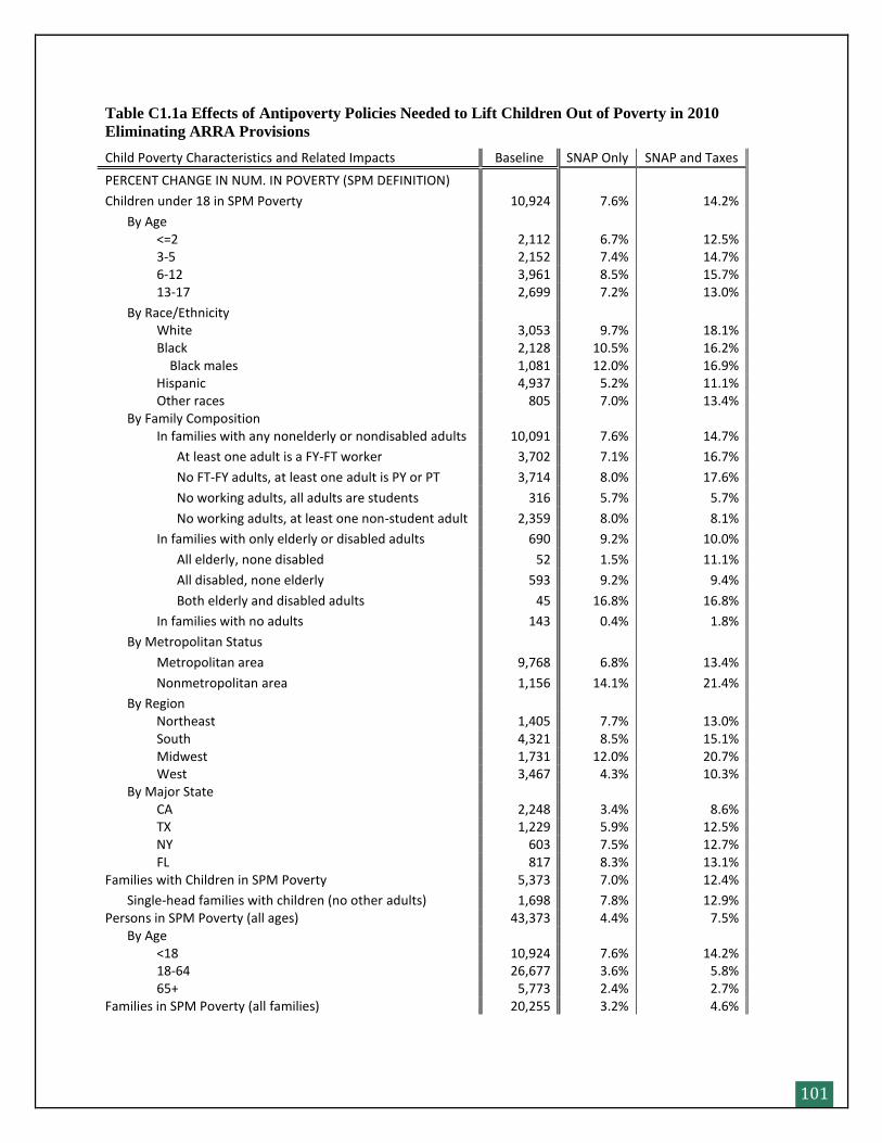
101
Table C1.1a Effects of Antipoverty Policies Needed to Lift Children Out of Poverty in 2010 Eliminating ARRA Provisions
Child Poverty Characteristics and Related Impacts Baseline SNAP Only SNAP and Taxes
PERCENT CHANGE IN NUM. IN POVERTY (SPM DEFINITION)
Children under 18 in SPM Poverty 10,924 7.6% 14.2%
By Age <=2 2,112 6.7% 12.5% 3-5 2,152 7.4% 14.7% 6-12 3,961 8.5% 15.7% 13-17 2,699 7.2% 13.0%
By Race/Ethnicity White 3,053 9.7% 18.1% Black 2,128 10.5% 16.2% Black males 1,081 12.0% 16.9% Hispanic 4,937 5.2% 11.1% Other races 805 7.0% 13.4% By Family Composition In families with any nonelderly or nondisabled adults 10,091 7.6% 14.7%
At least one adult is a FY-FT worker 3,702 7.1% 16.7%
No FT-FY adults, at least one adult is PY or PT 3,714 8.0% 17.6%
No working adults, all adults are students 316 5.7% 5.7%
No working adults, at least one non-student adult 2,359 8.0% 8.1%
In families with only elderly or disabled adults 690 9.2% 10.0%
All elderly, none disabled 52 1.5% 11.1%
All disabled, none elderly 593 9.2% 9.4%
Both elderly and disabled adults 45 16.8% 16.8%
In families with no adults 143 0.4% 1.8%
By Metropolitan Status
Metropolitan area 9,768 6.8% 13.4%
Nonmetropolitan area 1,156 14.1% 21.4%
By Region Northeast 1,405 7.7% 13.0% South 4,321 8.5% 15.1% Midwest 1,731 12.0% 20.7% West 3,467 4.3% 10.3% By Major State CA 2,248 3.4% 8.6% TX 1,229 5.9% 12.5% NY 603 7.5% 12.7% FL 817 8.3% 13.1% Families with Children in SPM Poverty 5,373 7.0% 12.4%
Single-head families with children (no other adults) 1,698 7.8% 12.9% Persons in SPM Poverty (all ages) 43,373 4.4% 7.5% By Age <18 10,924 7.6% 14.2% 18-64 26,677 3.6% 5.8% 65+ 5,773 2.4% 2.7% Families in SPM Poverty (all families) 20,255 3.2% 4.6%
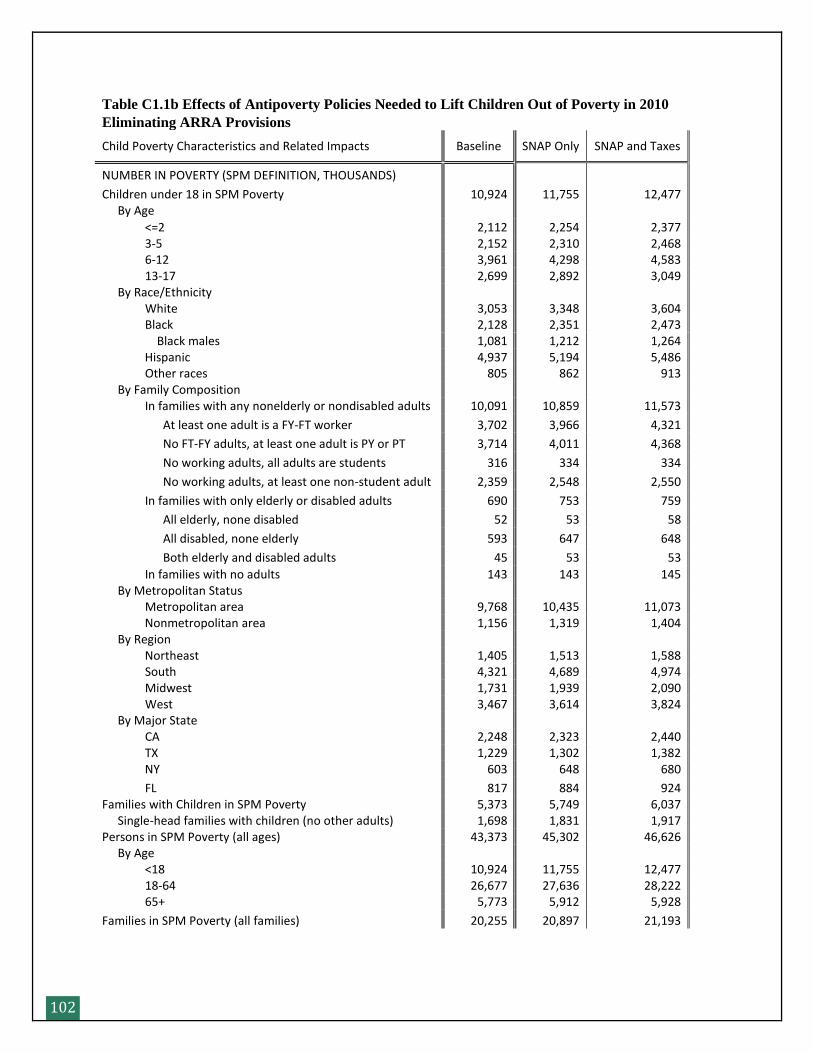
102
Table C1.1b Effects of Antipoverty Policies Needed to Lift Children Out of Poverty in 2010
Eliminating ARRA Provisions
Child Poverty Characteristics and Related Impacts Baseline SNAP Only SNAP and Taxes
NUMBER IN POVERTY (SPM DEFINITION, THOUSANDS)
Children under 18 in SPM Poverty 10,924 11,755 12,477 By Age
<=2 2,112 2,254 2,377 3-5 2,152 2,310 2,468 6-12 3,961 4,298 4,583 13-17 2,699 2,892 3,049 By Race/Ethnicity White 3,053 3,348 3,604 Black 2,128 2,351 2,473 Black males 1,081 1,212 1,264 Hispanic 4,937 5,194 5,486 Other races 805 862 913 By Family Composition In families with any nonelderly or nondisabled adults 10,091 10,859 11,573
At least one adult is a FY-FT worker 3,702 3,966 4,321
No FT-FY adults, at least one adult is PY or PT 3,714 4,011 4,368
No working adults, all adults are students 316 334 334
No working adults, at least one non-student adult 2,359 2,548 2,550
In families with only elderly or disabled adults 690 753 759
All elderly, none disabled 52 53 58
All disabled, none elderly 593 647 648
Both elderly and disabled adults 45 53 53
In families with no adults 143 143 145 By Metropolitan Status Metropolitan area 9,768 10,435 11,073 Nonmetropolitan area 1,156 1,319 1,404 By Region Northeast 1,405 1,513 1,588 South 4,321 4,689 4,974 Midwest 1,731 1,939 2,090 West 3,467 3,614 3,824 By Major State CA 2,248 2,323 2,440 TX 1,229 1,302 1,382 NY 603 648 680
FL 817 884 924 Families with Children in SPM Poverty 5,373 5,749 6,037 Single-head families with children (no other adults) 1,698 1,831 1,917 Persons in SPM Poverty (all ages) 43,373 45,302 46,626 By Age <18 10,924 11,755 12,477 18-64 26,677 27,636 28,222 65+ 5,773 5,912 5,928
Families in SPM Poverty (all families) 20,255 20,897 21,193
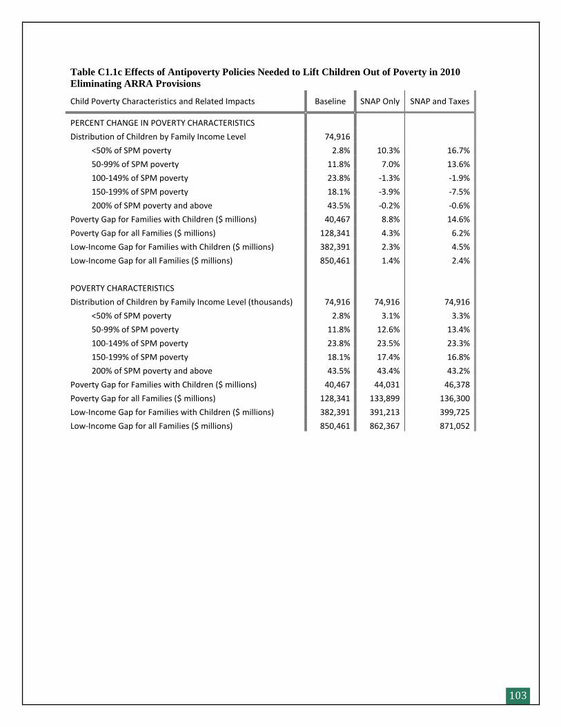
103
Table C1.1c Effects of Antipoverty Policies Needed to Lift Children Out of Poverty in 2010 Eliminating ARRA Provisions
Child Poverty Characteristics and Related Impacts Baseline SNAP Only SNAP and Taxes
PERCENT CHANGE IN POVERTY CHARACTERISTICS
Distribution of Children by Family Income Level 74,916
<50% of SPM poverty 2.8% 10.3% 16.7%
50-99% of SPM poverty 11.8% 7.0% 13.6%
100-149% of SPM poverty 23.8% -1.3% -1.9%
150-199% of SPM poverty 18.1% -3.9% -7.5%
200% of SPM poverty and above 43.5% -0.2% -0.6%
Poverty Gap for Families with Children ($ millions) 40,467 8.8% 14.6%
Poverty Gap for all Families ($ millions) 128,341 4.3% 6.2%
Low-Income Gap for Families with Children ($ millions) 382,391 2.3% 4.5%
Low-Income Gap for all Families ($ millions) 850,461 1.4% 2.4%
POVERTY CHARACTERISTICS
Distribution of Children by Family Income Level (thousands) 74,916 74,916 74,916
<50% of SPM poverty 2.8% 3.1% 3.3%
50-99% of SPM poverty 11.8% 12.6% 13.4%
100-149% of SPM poverty 23.8% 23.5% 23.3%
150-199% of SPM poverty 18.1% 17.4% 16.8%
200% of SPM poverty and above 43.5% 43.4% 43.2%
Poverty Gap for Families with Children ($ millions) 40,467 44,031 46,378
Poverty Gap for all Families ($ millions) 128,341 133,899 136,300
Low-Income Gap for Families with Children ($ millions) 382,391 391,213 399,725
Low-Income Gap for all Families ($ millions) 850,461 862,367 871,052
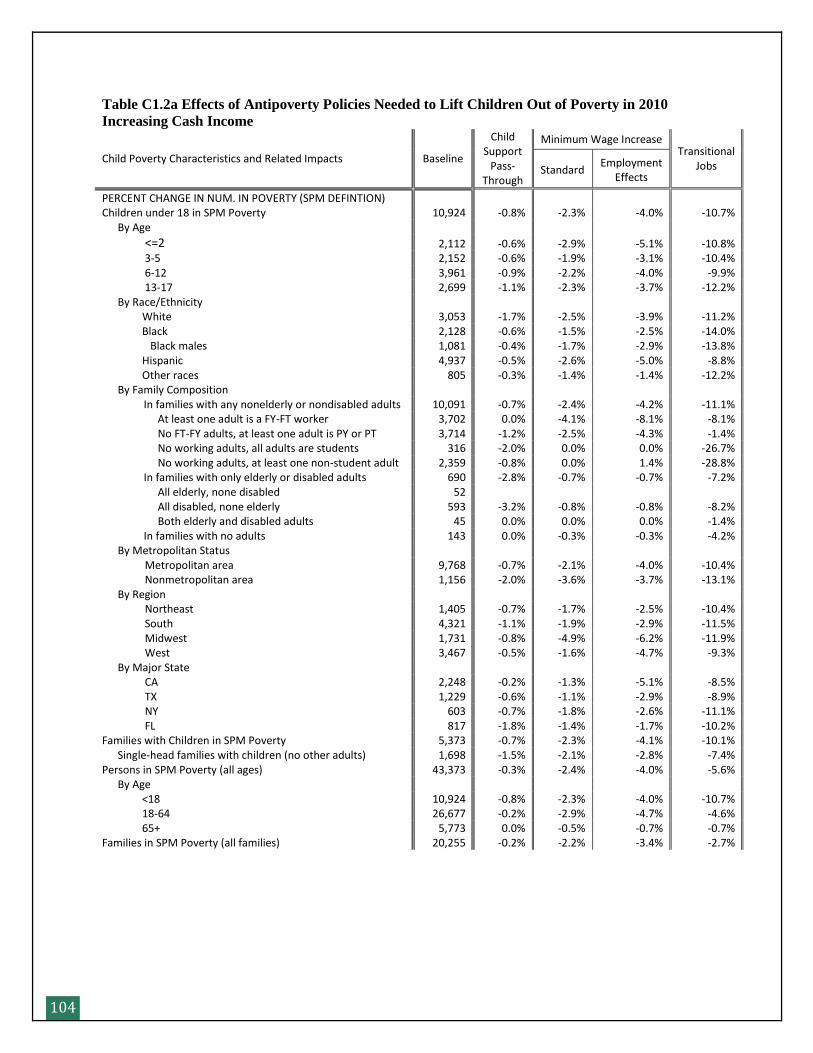
104
Table C1.2a Effects of Antipoverty Policies Needed to Lift Children Out of Poverty in 2010 Increasing Cash Income
Child Poverty Characteristics and Related Impacts Baseline
Child Support
Pass-Through
Minimum Wage Increase Transitional
Jobs Standard Employment
Effects
PERCENT CHANGE IN NUM. IN POVERTY (SPM DEFINTION) Children under 18 in SPM Poverty 10,924 -0.8% -2.3% -4.0% -10.7% By Age
<=2 2,112 -0.6% -2.9% -5.1% -10.8% 3-5 2,152 -0.6% -1.9% -3.1% -10.4% 6-12 3,961 -0.9% -2.2% -4.0% -9.9% 13-17 2,699 -1.1% -2.3% -3.7% -12.2% By Race/Ethnicity White 3,053 -1.7% -2.5% -3.9% -11.2% Black 2,128 -0.6% -1.5% -2.5% -14.0% Black males 1,081 -0.4% -1.7% -2.9% -13.8% Hispanic 4,937 -0.5% -2.6% -5.0% -8.8% Other races 805 -0.3% -1.4% -1.4% -12.2% By Family Composition In families with any nonelderly or nondisabled adults 10,091 -0.7% -2.4% -4.2% -11.1% At least one adult is a FY-FT worker 3,702 0.0% -4.1% -8.1% -8.1% No FT-FY adults, at least one adult is PY or PT 3,714 -1.2% -2.5% -4.3% -1.4% No working adults, all adults are students 316 -2.0% 0.0% 0.0% -26.7% No working adults, at least one non-student adult 2,359 -0.8% 0.0% 1.4% -28.8% In families with only elderly or disabled adults 690 -2.8% -0.7% -0.7% -7.2% All elderly, none disabled 52 All disabled, none elderly 593 -3.2% -0.8% -0.8% -8.2% Both elderly and disabled adults 45 0.0% 0.0% 0.0% -1.4% In families with no adults 143 0.0% -0.3% -0.3% -4.2% By Metropolitan Status Metropolitan area 9,768 -0.7% -2.1% -4.0% -10.4% Nonmetropolitan area 1,156 -2.0% -3.6% -3.7% -13.1% By Region Northeast 1,405 -0.7% -1.7% -2.5% -10.4% South 4,321 -1.1% -1.9% -2.9% -11.5% Midwest 1,731 -0.8% -4.9% -6.2% -11.9% West 3,467 -0.5% -1.6% -4.7% -9.3% By Major State CA 2,248 -0.2% -1.3% -5.1% -8.5% TX 1,229 -0.6% -1.1% -2.9% -8.9% NY 603 -0.7% -1.8% -2.6% -11.1% FL 817 -1.8% -1.4% -1.7% -10.2% Families with Children in SPM Poverty 5,373 -0.7% -2.3% -4.1% -10.1% Single-head families with children (no other adults) 1,698 -1.5% -2.1% -2.8% -7.4% Persons in SPM Poverty (all ages) 43,373 -0.3% -2.4% -4.0% -5.6% By Age <18 10,924 -0.8% -2.3% -4.0% -10.7% 18-64 26,677 -0.2% -2.9% -4.7% -4.6% 65+ 5,773 0.0% -0.5% -0.7% -0.7% Families in SPM Poverty (all families) 20,255 -0.2% -2.2% -3.4% -2.7%
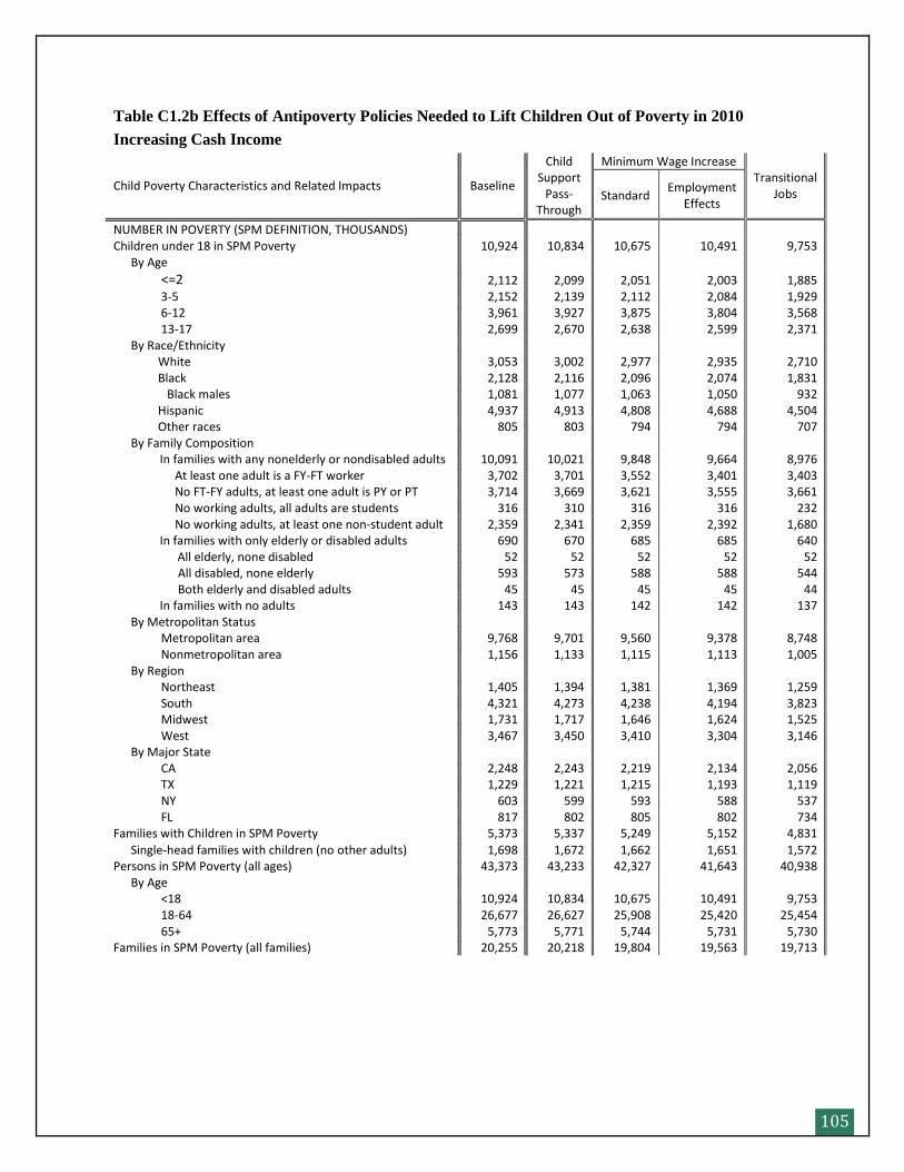
105
Table C1.2b Effects of Antipoverty Policies Needed to Lift Children Out of Poverty in 2010
Increasing Cash Income
Child Poverty Characteristics and Related Impacts Baseline
Child Support
Pass-Through
Minimum Wage Increase Transitional
Jobs Standard Employment
Effects
NUMBER IN POVERTY (SPM DEFINITION, THOUSANDS) Children under 18 in SPM Poverty 10,924 10,834 10,675 10,491 9,753 By Age
<=2 2,112 2,099 2,051 2,003 1,885 3-5 2,152 2,139 2,112 2,084 1,929 6-12 3,961 3,927 3,875 3,804 3,568 13-17 2,699 2,670 2,638 2,599 2,371 By Race/Ethnicity White 3,053 3,002 2,977 2,935 2,710 Black 2,128 2,116 2,096 2,074 1,831 Black males 1,081 1,077 1,063 1,050 932 Hispanic 4,937 4,913 4,808 4,688 4,504 Other races 805 803 794 794 707 By Family Composition In families with any nonelderly or nondisabled adults 10,091 10,021 9,848 9,664 8,976 At least one adult is a FY-FT worker 3,702 3,701 3,552 3,401 3,403 No FT-FY adults, at least one adult is PY or PT 3,714 3,669 3,621 3,555 3,661 No working adults, all adults are students 316 310 316 316 232 No working adults, at least one non-student adult 2,359 2,341 2,359 2,392 1,680 In families with only elderly or disabled adults 690 670 685 685 640 All elderly, none disabled 52 52 52 52 52 All disabled, none elderly 593 573 588 588 544 Both elderly and disabled adults 45 45 45 45 44 In families with no adults 143 143 142 142 137 By Metropolitan Status Metropolitan area 9,768 9,701 9,560 9,378 8,748 Nonmetropolitan area 1,156 1,133 1,115 1,113 1,005 By Region Northeast 1,405 1,394 1,381 1,369 1,259 South 4,321 4,273 4,238 4,194 3,823 Midwest 1,731 1,717 1,646 1,624 1,525 West 3,467 3,450 3,410 3,304 3,146 By Major State CA 2,248 2,243 2,219 2,134 2,056 TX 1,229 1,221 1,215 1,193 1,119 NY 603 599 593 588 537 FL 817 802 805 802 734 Families with Children in SPM Poverty 5,373 5,337 5,249 5,152 4,831
Single-head families with children (no other adults) 1,698 1,672 1,662 1,651 1,572 Persons in SPM Poverty (all ages) 43,373 43,233 42,327 41,643 40,938 By Age <18 10,924 10,834 10,675 10,491 9,753 18-64 26,677 26,627 25,908 25,420 25,454 65+ 5,773 5,771 5,744 5,731 5,730 Families in SPM Poverty (all families) 20,255 20,218 19,804 19,563 19,713
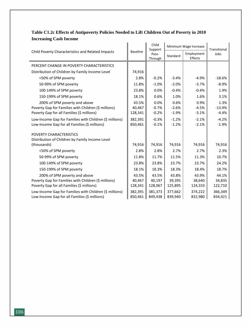
106
Table C1.2c Effects of Antipoverty Policies Needed to Lift Children Out of Poverty in 2010
Increasing Cash Income
Child Poverty Characteristics and Related Impacts Baseline
Child Support
Pass-Through
Minimum Wage Increase Transitional
Jobs Standard
Employment Effects
PERCENT CHANGE IN POVERTY CHARACTERISTICS
Distribution of Children by Family Income Level 74,916
<50% of SPM poverty 2.8% -0.2% -3.4% -4.9% -18.6%
50-99% of SPM poverty 11.8% -1.0% -2.0% -3.7% -8.9%
100-149% of SPM poverty 23.8% 0.0% -0.4% -0.4% 1.9%
150-199% of SPM poverty 18.1% 0.6% 1.0% 1.6% 3.1%
200% of SPM poverty and above 43.5% 0.0% 0.6% 0.9% 1.3% Poverty Gap for Families with Children ($ millions) 40,467 -0.7% -2.6% -4.5% -13.9% Poverty Gap for all Families ($ millions) 128,341 -0.2% -1.9% -3.1% -4.4%
Low-Income Gap for Families with Children ($ millions) 382,391 -0.3% -1.2% -2.1% -4.2% Low-Income Gap for all Families ($ millions) 850,461 -0.1% -1.2% -2.1% -1.9% POVERTY CHARACTERISTICS Distribution of Children by Family Income Level (thousands) 74,916 74,916 74,916 74,916 74,916
<50% of SPM poverty 2.8% 2.8% 2.7% 2.7% 2.3%
50-99% of SPM poverty 11.8% 11.7% 11.5% 11.3% 10.7%
100-149% of SPM poverty 23.8% 23.8% 23.7% 23.7% 24.2%
150-199% of SPM poverty 18.1% 18.3% 18.3% 18.4% 18.7%
200% of SPM poverty and above 43.5% 43.5% 43.8% 43.9% 44.1% Poverty Gap for Families with Children ($ millions) 40,467 40,197 39,395 38,640 34,835 Poverty Gap for all Families ($ millions) 128,341 128,067 125,895 124,333 122,710
Low-Income Gap for Families with Children ($ millions) 382,391 381,373 377,662 374,222 366,349 Low-Income Gap for all Families ($ millions) 850,461 849,438 839,940 832,980 834,421
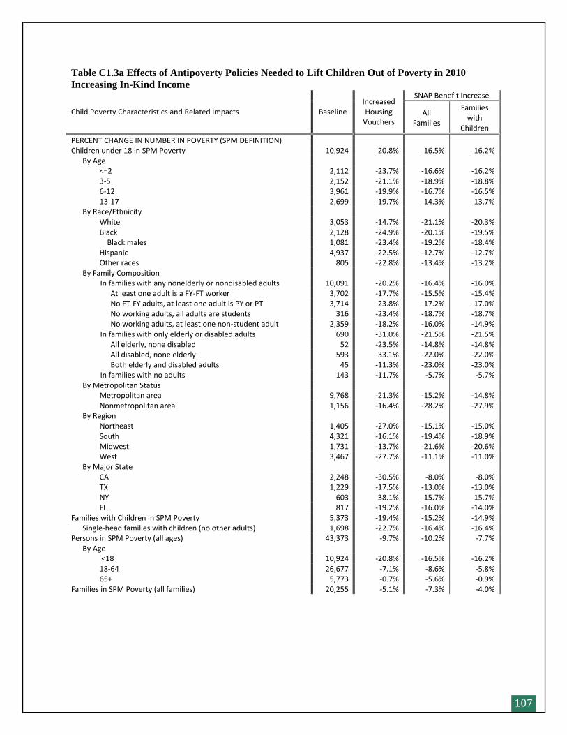
107
Table C1.3a Effects of Antipoverty Policies Needed to Lift Children Out of Poverty in 2010 Increasing In-Kind Income
Child Poverty Characteristics and Related Impacts Baseline Increased Housing
Vouchers
SNAP Benefit Increase
All Families
Families with
Children
PERCENT CHANGE IN NUMBER IN POVERTY (SPM DEFINITION) Children under 18 in SPM Poverty 10,924 -20.8% -16.5% -16.2% By Age <=2 2,112 -23.7% -16.6% -16.2% 3-5 2,152 -21.1% -18.9% -18.8% 6-12 3,961 -19.9% -16.7% -16.5% 13-17 2,699 -19.7% -14.3% -13.7% By Race/Ethnicity White 3,053 -14.7% -21.1% -20.3% Black 2,128 -24.9% -20.1% -19.5% Black males 1,081 -23.4% -19.2% -18.4% Hispanic 4,937 -22.5% -12.7% -12.7% Other races 805 -22.8% -13.4% -13.2% By Family Composition In families with any nonelderly or nondisabled adults 10,091 -20.2% -16.4% -16.0% At least one adult is a FY-FT worker 3,702 -17.7% -15.5% -15.4% No FT-FY adults, at least one adult is PY or PT 3,714 -23.8% -17.2% -17.0% No working adults, all adults are students 316 -23.4% -18.7% -18.7% No working adults, at least one non-student adult 2,359 -18.2% -16.0% -14.9% In families with only elderly or disabled adults 690 -31.0% -21.5% -21.5% All elderly, none disabled 52 -23.5% -14.8% -14.8% All disabled, none elderly 593 -33.1% -22.0% -22.0% Both elderly and disabled adults 45 -11.3% -23.0% -23.0% In families with no adults 143 -11.7% -5.7% -5.7% By Metropolitan Status Metropolitan area 9,768 -21.3% -15.2% -14.8% Nonmetropolitan area 1,156 -16.4% -28.2% -27.9% By Region Northeast 1,405 -27.0% -15.1% -15.0% South 4,321 -16.1% -19.4% -18.9% Midwest 1,731 -13.7% -21.6% -20.6% West 3,467 -27.7% -11.1% -11.0% By Major State CA 2,248 -30.5% -8.0% -8.0% TX 1,229 -17.5% -13.0% -13.0% NY 603 -38.1% -15.7% -15.7% FL 817 -19.2% -16.0% -14.0% Families with Children in SPM Poverty 5,373 -19.4% -15.2% -14.9% Single-head families with children (no other adults) 1,698 -22.7% -16.4% -16.4% Persons in SPM Poverty (all ages) 43,373 -9.7% -10.2% -7.7% By Age <18 10,924 -20.8% -16.5% -16.2% 18-64 26,677 -7.1% -8.6% -5.8% 65+ 5,773 -0.7% -5.6% -0.9% Families in SPM Poverty (all families) 20,255 -5.1% -7.3% -4.0%
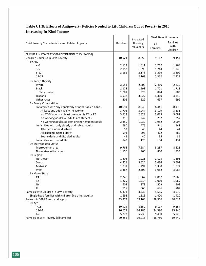
108
Table C1.3b Effects of Antipoverty Policies Needed to Lift Children Out of Poverty in 2010
Increasing In-Kind Income
Child Poverty Characteristics and Related Impacts Baseline Increased Housing
Vouchers
SNAP Benefit Increase
All Families
Families with
Children
NUMBER IN POVERTY (SPM DEFINITION, THOUSANDS) Children under 18 in SPM Poverty 10,924 8,650 9,117 9,154 By Age <=2 2,112 1,611 1,762 1,769 3-5 2,152 1,698 1,744 1,748 6-12 3,961 3,173 3,299 3,309 13-17 2,168 2,312 2,328
By Race/Ethnicity White 3,053 2,603 2,410 2,432 Black 2,128 1,598 1,701 1,713 Black males 1,081 828 874 883 Hispanic 4,937 3,827 4,310 4,310 Other races 805 622 697 699 By Family Composition In families with any nonelderly or nondisabled adults 10,091 8,048 8,441 8,478 At least one adult is a FY-FT worker 3,702 3,047 3,129 3,133 No FT-FY adults, at least one adult is PY or PT 3,714 2,829 3,073 3,081 No working adults, all adults are students 316 242 257 257 No working adults, at least one non-student adult 2,359 1,930 1,982 2,007 In families with only elderly or disabled adults 690 476 541 541 All elderly, none disabled 52 40 44 44 All disabled, none elderly 593 396 462 462 Both elderly and disabled adults 45 40 35 35 In families with no adults 143 126 134 134 By Metropolitan Status Metropolitan area 9,768 7,684 8,287 8,321 Nonmetropolitan area 1,156 966 830 833 By Region Northeast 1,405 1,025 1,193 1,193 South 4,321 3,624 3,484 3,502 Midwest 1,731 1,494 1,358 1,374 West 3,467 2,507 3,082 3,084 By Major State CA 2,248 1,562 2,067 2,069 TX 1,229 1,014 1,069 1,069 NY 603 373 509 509 FL 817 660 686 702 Families with Children in SPM Poverty 5,373 4,333 4,555 4,570 Single-head families with children (no other adults) 1,698 1,313 1,420 1,420 Persons in SPM Poverty (all ages) 43,373 39,168 38,956 40,014 By Age <18 10,924 8,650 9,117 9,154 18-64 26,677 24,785 24,390 25,140 65+ 5,773 5,733 5,450 5,720 Families in SPM Poverty (all families) 20,255 19,213 18,780 19,449
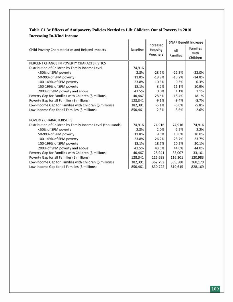
109
Table C1.3c Effects of Antipoverty Policies Needed to Lift Children Out of Poverty in 2010
Increasing In-Kind Income
Child Poverty Characteristics and Related Impacts Baseline Increased Housing
Vouchers
SNAP Benefit Increase
All Families
Families with
Children
PERCENT CHANGE IN POVERTY CHARACTERISTICS Distribution of Children by Family Income Level 74,916 <50% of SPM poverty 2.8% -28.7% -22.3% -22.0% 50-99% of SPM poverty 11.8% -18.9% -15.2% -14.8% 100-149% of SPM poverty 23.8% 10.3% -0.3% -0.3% 150-199% of SPM poverty 18.1% 3.2% 11.1% 10.9% 200% of SPM poverty and above 43.5% 0.0% 1.1% 1.1% Poverty Gap for Families with Children ($ millions) 40,467 -28.5% -18.4% -18.1% Poverty Gap for all Families ($ millions) 128,341 -9.1% -9.4% -5.7% Low-Income Gap for Families with Children ($ millions) 382,391 -5.1% -6.0% -5.8% Low-Income Gap for all Families ($ millions) 850,461 -2.3% -3.6% -2.6%
POVERTY CHARACTERISTICS Distribution of Children by Family Income Level (thousands) 74,916 74,916 74,916 74,916 <50% of SPM poverty 2.8% 2.0% 2.2% 2.2% 50-99% of SPM poverty 11.8% 9.5% 10.0% 10.0% 100-149% of SPM poverty 23.8% 26.2% 23.7% 23.7% 150-199% of SPM poverty 18.1% 18.7% 20.2% 20.1% 200% of SPM poverty and above 43.5% 43.5% 44.0% 44.0% Poverty Gap for Families with Children ($ millions) 40,467 28,941 33,007 33,161 Poverty Gap for all Families ($ millions) 128,341 116,698 116,301 120,983 Low-Income Gap for Families with Children ($ millions) 382,391 362,792 359,588 360,179 Low-Income Gap for all Families ($ millions) 850,461 830,722 819,615 828,169
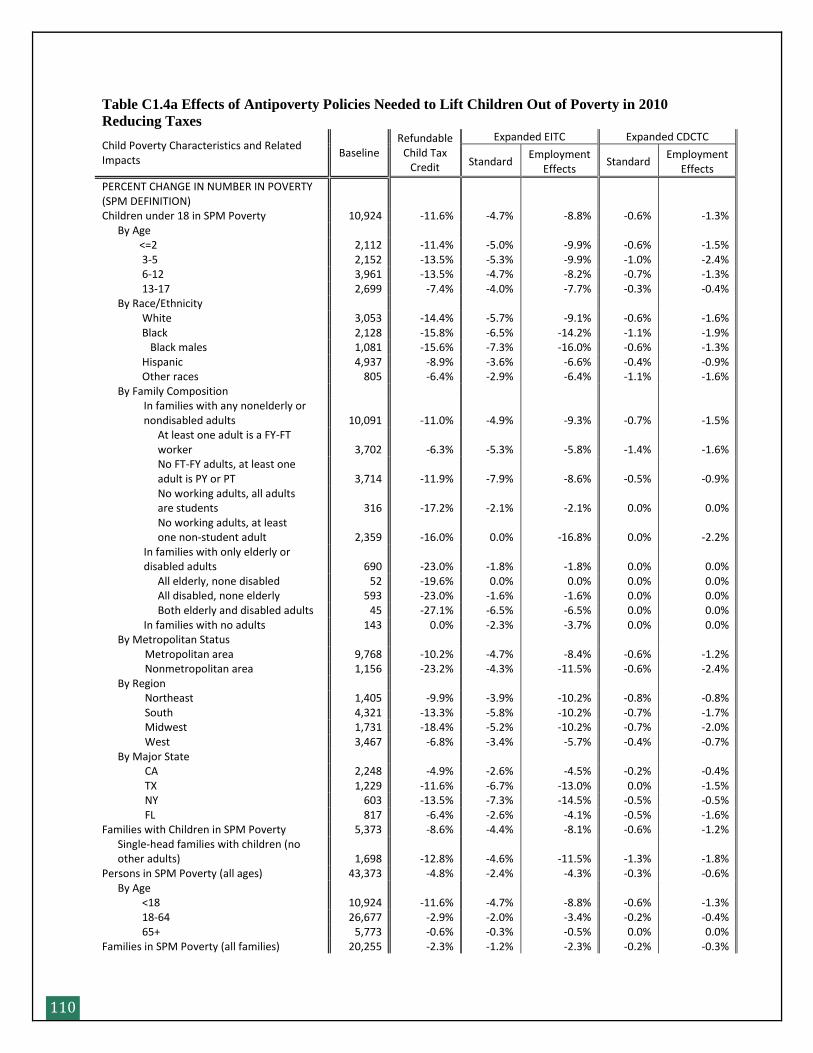
110
Table C1.4a Effects of Antipoverty Policies Needed to Lift Children Out of Poverty in 2010 Reducing Taxes
Child Poverty Characteristics and Related Impacts
Baseline Refundable
Child Tax Credit
Expanded EITC Expanded CDCTC
Standard Employment
Effects Standard
Employment Effects
PERCENT CHANGE IN NUMBER IN POVERTY (SPM DEFINITION)
Children under 18 in SPM Poverty 10,924 -11.6% -4.7% -8.8% -0.6% -1.3% By Age <=2 2,112 -11.4% -5.0% -9.9% -0.6% -1.5% 3-5 2,152 -13.5% -5.3% -9.9% -1.0% -2.4% 6-12 3,961 -13.5% -4.7% -8.2% -0.7% -1.3% 13-17 2,699 -7.4% -4.0% -7.7% -0.3% -0.4% By Race/Ethnicity White 3,053 -14.4% -5.7% -9.1% -0.6% -1.6% Black 2,128 -15.8% -6.5% -14.2% -1.1% -1.9% Black males 1,081 -15.6% -7.3% -16.0% -0.6% -1.3% Hispanic 4,937 -8.9% -3.6% -6.6% -0.4% -0.9% Other races 805 -6.4% -2.9% -6.4% -1.1% -1.6% By Family Composition
In families with any nonelderly or nondisabled adults 10,091 -11.0% -4.9% -9.3% -0.7% -1.5%
At least one adult is a FY-FT worker 3,702 -6.3% -5.3% -5.8% -1.4% -1.6%
No FT-FY adults, at least one adult is PY or PT 3,714 -11.9% -7.9% -8.6% -0.5% -0.9%
No working adults, all adults are students 316 -17.2% -2.1% -2.1% 0.0% 0.0%
No working adults, at least one non-student adult 2,359 -16.0% 0.0% -16.8% 0.0% -2.2%
In families with only elderly or disabled adults 690 -23.0% -1.8% -1.8% 0.0% 0.0%
All elderly, none disabled 52 -19.6% 0.0% 0.0% 0.0% 0.0% All disabled, none elderly 593 -23.0% -1.6% -1.6% 0.0% 0.0% Both elderly and disabled adults 45 -27.1% -6.5% -6.5% 0.0% 0.0% In families with no adults 143 0.0% -2.3% -3.7% 0.0% 0.0% By Metropolitan Status Metropolitan area 9,768 -10.2% -4.7% -8.4% -0.6% -1.2% Nonmetropolitan area 1,156 -23.2% -4.3% -11.5% -0.6% -2.4% By Region Northeast 1,405 -9.9% -3.9% -10.2% -0.8% -0.8% South 4,321 -13.3% -5.8% -10.2% -0.7% -1.7% Midwest 1,731 -18.4% -5.2% -10.2% -0.7% -2.0% West 3,467 -6.8% -3.4% -5.7% -0.4% -0.7% By Major State CA 2,248 -4.9% -2.6% -4.5% -0.2% -0.4% TX 1,229 -11.6% -6.7% -13.0% 0.0% -1.5% NY 603 -13.5% -7.3% -14.5% -0.5% -0.5% FL 817 -6.4% -2.6% -4.1% -0.5% -1.6% Families with Children in SPM Poverty 5,373 -8.6% -4.4% -8.1% -0.6% -1.2%
Single-head families with children (no other adults) 1,698 -12.8% -4.6% -11.5% -1.3% -1.8%
Persons in SPM Poverty (all ages) 43,373 -4.8% -2.4% -4.3% -0.3% -0.6% By Age <18 10,924 -11.6% -4.7% -8.8% -0.6% -1.3% 18-64 26,677 -2.9% -2.0% -3.4% -0.2% -0.4% 65+ 5,773 -0.6% -0.3% -0.5% 0.0% 0.0% Families in SPM Poverty (all families) 20,255 -2.3% -1.2% -2.3% -0.2% -0.3%
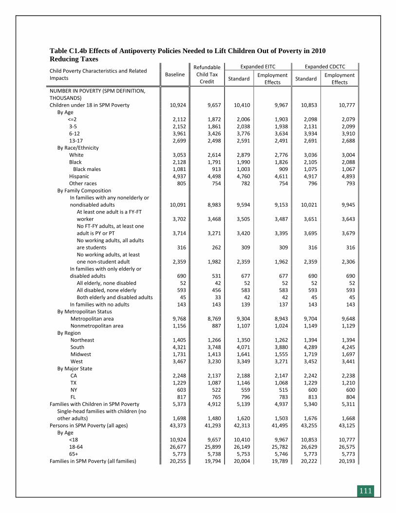
111
Table C1.4b Effects of Antipoverty Policies Needed to Lift Children Out of Poverty in 2010 Reducing Taxes
Child Poverty Characteristics and Related Impacts
Baseline Refundable
Child Tax Credit
Expanded EITC Expanded CDCTC
Standard Employment
Effects Standard
Employment Effects
NUMBER IN POVERTY (SPM DEFINITION, THOUSANDS) Children under 18 in SPM Poverty 10,924 9,657 10,410 9,967 10,853 10,777 By Age <=2 2,112 1,872 2,006 1,903 2,098 2,079 3-5 2,152 1,861 2,038 1,938 2,131 2,099 6-12 3,961 3,426 3,776 3,634 3,934 3,910 13-17 2,699 2,498 2,591 2,491 2,691 2,688 By Race/Ethnicity White 3,053 2,614 2,879 2,776 3,036 3,004 Black 2,128 1,791 1,990 1,826 2,105 2,088 Black males 1,081 913 1,003 909 1,075 1,067 Hispanic 4,937 4,498 4,760 4,611 4,917 4,893 Other races 805 754 782 754 796 793 By Family Composition
In families with any nonelderly or nondisabled adults 10,091 8,983 9,594 9,153 10,021 9,945
At least one adult is a FY-FT worker 3,702 3,468 3,505 3,487 3,651 3,643
No FT-FY adults, at least one adult is PY or PT 3,714 3,271 3,420 3,395 3,695 3,679
No working adults, all adults are students 316 262 309 309 316 316
No working adults, at least one non-student adult 2,359 1,982 2,359 1,962 2,359 2,306
In families with only elderly or disabled adults 690 531 677 677 690 690
All elderly, none disabled 52 42 52 52 52 52 All disabled, none elderly 593 456 583 583 593 593 Both elderly and disabled adults 45 33 42 42 45 45 In families with no adults 143 143 139 137 143 143 By Metropolitan Status Metropolitan area 9,768 8,769 9,304 8,943 9,704 9,648 Nonmetropolitan area 1,156 887 1,107 1,024 1,149 1,129 By Region Northeast 1,405 1,266 1,350 1,262 1,394 1,394 South 4,321 3,748 4,071 3,880 4,289 4,245 Midwest 1,731 1,413 1,641 1,555 1,719 1,697 West 3,467 3,230 3,349 3,271 3,452 3,441 By Major State CA 2,248 2,137 2,188 2,147 2,242 2,238 TX 1,229 1,087 1,146 1,068 1,229 1,210 NY 603 522 559 515 600 600 FL 817 765 796 783 813 804 Families with Children in SPM Poverty 5,373 4,912 5,139 4,937 5,340 5,311
Single-head families with children (no other adults) 1,698 1,480 1,620 1,503 1,676 1,668
Persons in SPM Poverty (all ages) 43,373 41,293 42,313 41,495 43,255 43,125 By Age <18 10,924 9,657 10,410 9,967 10,853 10,777 18-64 26,677 25,899 26,149 25,782 26,629 26,575 65+ 5,773 5,738 5,753 5,746 5,773 5,773 Families in SPM Poverty (all families) 20,255 19,794 20,004 19,789 20,222 20,193
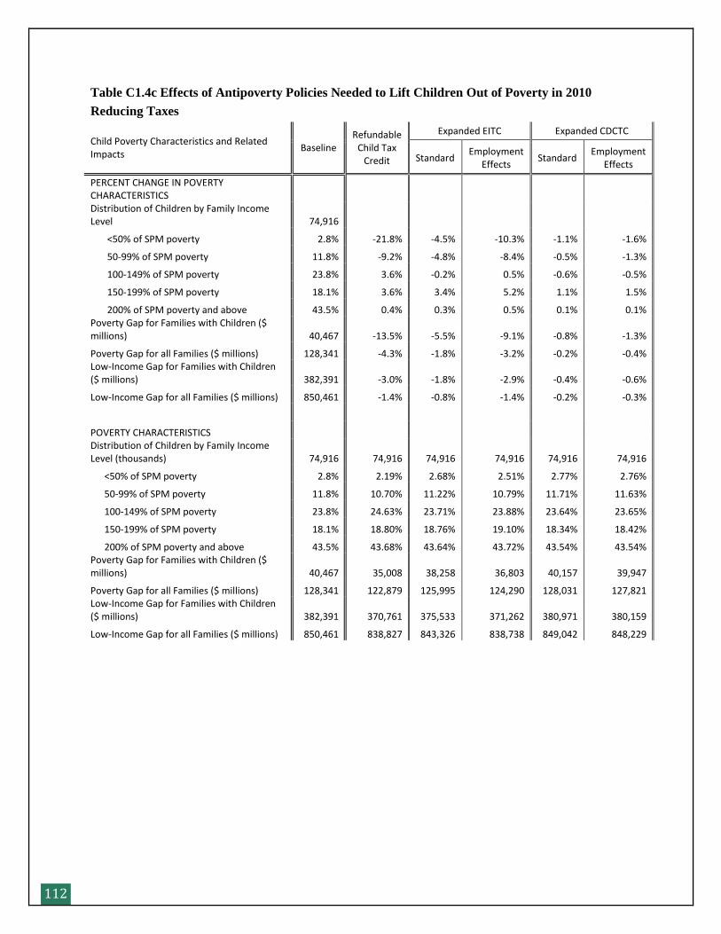
112
Table C1.4c Effects of Antipoverty Policies Needed to Lift Children Out of Poverty in 2010
Reducing Taxes
Child Poverty Characteristics and Related Impacts
Baseline Refundable
Child Tax Credit
Expanded EITC Expanded CDCTC
Standard Employment
Effects Standard
Employment Effects
PERCENT CHANGE IN POVERTY CHARACTERISTICS Distribution of Children by Family Income Level 74,916
<50% of SPM poverty 2.8% -21.8% -4.5% -10.3% -1.1% -1.6%
50-99% of SPM poverty 11.8% -9.2% -4.8% -8.4% -0.5% -1.3%
100-149% of SPM poverty 23.8% 3.6% -0.2% 0.5% -0.6% -0.5%
150-199% of SPM poverty 18.1% 3.6% 3.4% 5.2% 1.1% 1.5%
200% of SPM poverty and above 43.5% 0.4% 0.3% 0.5% 0.1% 0.1% Poverty Gap for Families with Children ($ millions) 40,467 -13.5% -5.5% -9.1% -0.8% -1.3%
Poverty Gap for all Families ($ millions) 128,341 -4.3% -1.8% -3.2% -0.2% -0.4% Low-Income Gap for Families with Children ($ millions) 382,391 -3.0% -1.8% -2.9% -0.4% -0.6%
Low-Income Gap for all Families ($ millions) 850,461 -1.4% -0.8% -1.4% -0.2% -0.3%
POVERTY CHARACTERISTICS Distribution of Children by Family Income Level (thousands) 74,916 74,916 74,916 74,916 74,916 74,916
<50% of SPM poverty 2.8% 2.19% 2.68% 2.51% 2.77% 2.76%
50-99% of SPM poverty 11.8% 10.70% 11.22% 10.79% 11.71% 11.63%
100-149% of SPM poverty 23.8% 24.63% 23.71% 23.88% 23.64% 23.65%
150-199% of SPM poverty 18.1% 18.80% 18.76% 19.10% 18.34% 18.42%
200% of SPM poverty and above 43.5% 43.68% 43.64% 43.72% 43.54% 43.54% Poverty Gap for Families with Children ($ millions) 40,467 35,008 38,258 36,803 40,157 39,947
Poverty Gap for all Families ($ millions) 128,341 122,879 125,995 124,290 128,031 127,821 Low-Income Gap for Families with Children ($ millions) 382,391 370,761 375,533 371,262 380,971 380,159
Low-Income Gap for all Families ($ millions) 850,461 838,827 843,326 838,738 849,042 848,229
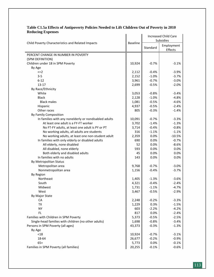
113
Table C1.5a Effects of Antipoverty Policies Needed to Lift Children Out of Poverty in 2010 Reducing Expenses
Child Poverty Characteristics and Related Impacts Baseline
Increased Child Care Subsidies
Standard Employment
Effects
PERCENT CHANGE IN NUMBER IN POVERTY (SPM DEFINITION)
Children under 18 in SPM Poverty 10,924 -0.7% -3.1% By Age <=2 2,112 -0.4% -3.9% 3-5 2,152 -1.0% -3.7% 6-12 3,961 -0.7% -3.0% 13-17 2,699 -0.5% -2.0% By Race/Ethnicity White 3,053 -0.8% -3.4% Black 2,128 -1.0% -4.8% Black males 1,081 -0.5% -4.6% Hispanic 4,937 -0.5% -2.4% Other races 805 -0.3% -1.4% By Family Composition In families with any nonelderly or nondisabled adults 10,091 -0.7% -3.3% At least one adult is a FY-FT worker 3,702 -1.4% -1.3% No FT-FY adults, at least one adult is PY or PT 3,714 -0.4% -0.8% No working adults, all adults are students 316 -1.1% -1.1% No working adults, at least one non-student adult 2,359 0.0% -10.5% In families with only elderly or disabled adults 690 0.0% -0.7% All elderly, none disabled 52 0.0% -8.6% All disabled, none elderly 593 0.0% 0.0% Both elderly and disabled adults 45 0.0% 0.0% In families with no adults 143 0.0% 0.0% By Metropolitan Status Metropolitan area 9,768 -0.7% -3.0% Nonmetropolitan area 1,156 -0.4% -3.7% By Region Northeast 1,405 -1.3% -3.6% South 4,321 -0.4% -2.4% Midwest 1,731 -1.1% -4.7% West 3,467 -0.5% -2.9% By Major State CA 2,248 -0.2% -3.3% TX 1,229 0.3% -1.5% NY 603 -2.2% -4.2% FL 817 0.0% -2.4% Families with Children in SPM Poverty 5,373 -0.5% -2.5% Single-head families with children (no other adults) 1,698 -0.8% -3.4% Persons in SPM Poverty (all ages) 43,373 -0.3% -1.3% By Age <18 10,924 -0.7% -3.1% 18-64 26,677 -0.2% -0.9% 65+ 5,773 0.0% -0.1% Families in SPM Poverty (all families) 20,255 -0.1% -0.6%
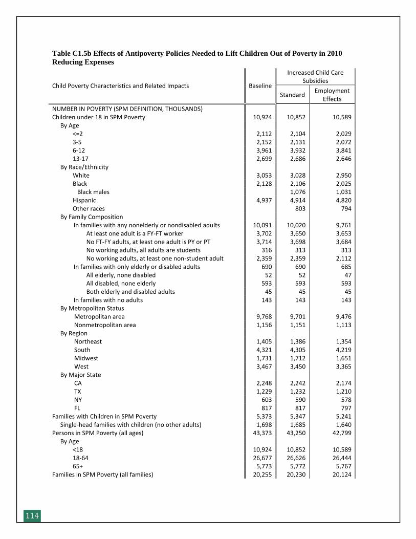
114
Table C1.5b Effects of Antipoverty Policies Needed to Lift Children Out of Poverty in 2010 Reducing Expenses
Child Poverty Characteristics and Related Impacts Baseline
Increased Child Care Subsidies
Standard Employment
Effects
NUMBER IN POVERTY (SPM DEFINITION, THOUSANDS) Children under 18 in SPM Poverty 10,924 10,852 10,589 By Age <=2 2,112 2,104 2,029 3-5 2,152 2,131 2,072 6-12 3,961 3,932 3,841 13-17 2,699 2,686 2,646 By Race/Ethnicity White 3,053 3,028 2,950 Black 2,128 2,106 2,025 Black males 1,076 1,031 Hispanic 4,937 4,914 4,820 Other races 803 794 By Family Composition In families with any nonelderly or nondisabled adults 10,091 10,020 9,761 At least one adult is a FY-FT worker 3,702 3,650 3,653 No FT-FY adults, at least one adult is PY or PT 3,714 3,698 3,684 No working adults, all adults are students 316 313 313 No working adults, at least one non-student adult 2,359 2,359 2,112 In families with only elderly or disabled adults 690 690 685 All elderly, none disabled 52 52 47 All disabled, none elderly 593 593 593 Both elderly and disabled adults 45 45 45 In families with no adults 143 143 143 By Metropolitan Status Metropolitan area 9,768 9,701 9,476 Nonmetropolitan area 1,156 1,151 1,113 By Region Northeast 1,405 1,386 1,354 South 4,321 4,305 4,219 Midwest 1,731 1,712 1,651 West 3,467 3,450 3,365 By Major State CA 2,248 2,242 2,174 TX 1,229 1,232 1,210 NY 603 590 578 FL 817 817 797 Families with Children in SPM Poverty 5,373 5,347 5,241 Single-head families with children (no other adults) 1,698 1,685 1,640 Persons in SPM Poverty (all ages) 43,373 43,250 42,799 By Age <18 10,924 10,852 10,589 18-64 26,677 26,626 26,444 65+ 5,773 5,772 5,767 Families in SPM Poverty (all families) 20,255 20,230 20,124
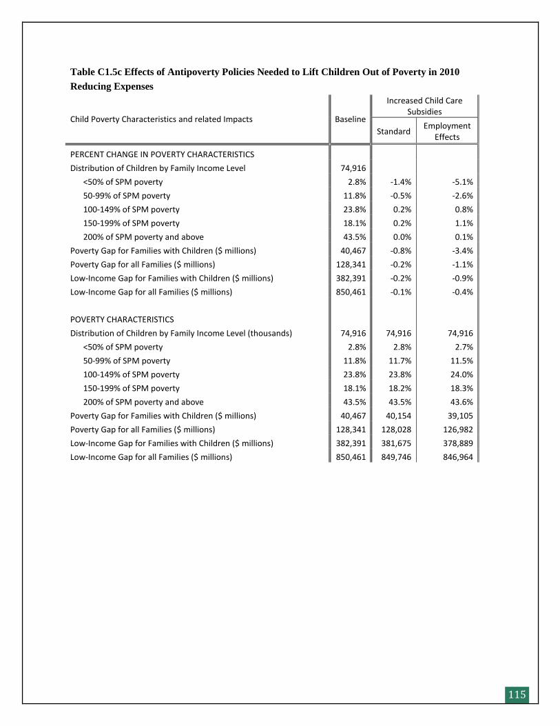
115
Table C1.5c Effects of Antipoverty Policies Needed to Lift Children Out of Poverty in 2010
Reducing Expenses
Child Poverty Characteristics and related Impacts Baseline
Increased Child Care Subsidies
Standard Employment
Effects
PERCENT CHANGE IN POVERTY CHARACTERISTICS
Distribution of Children by Family Income Level 74,916
<50% of SPM poverty 2.8% -1.4% -5.1%
50-99% of SPM poverty 11.8% -0.5% -2.6%
100-149% of SPM poverty 23.8% 0.2% 0.8%
150-199% of SPM poverty 18.1% 0.2% 1.1%
200% of SPM poverty and above 43.5% 0.0% 0.1%
Poverty Gap for Families with Children ($ millions) 40,467 -0.8% -3.4%
Poverty Gap for all Families ($ millions) 128,341 -0.2% -1.1%
Low-Income Gap for Families with Children ($ millions) 382,391 -0.2% -0.9%
Low-Income Gap for all Families ($ millions) 850,461 -0.1% -0.4%
POVERTY CHARACTERISTICS
Distribution of Children by Family Income Level (thousands) 74,916 74,916 74,916
<50% of SPM poverty 2.8% 2.8% 2.7%
50-99% of SPM poverty 11.8% 11.7% 11.5%
100-149% of SPM poverty 23.8% 23.8% 24.0%
150-199% of SPM poverty 18.1% 18.2% 18.3%
200% of SPM poverty and above 43.5% 43.5% 43.6%
Poverty Gap for Families with Children ($ millions) 40,467 40,154 39,105
Poverty Gap for all Families ($ millions) 128,341 128,028 126,982
Low-Income Gap for Families with Children ($ millions) 382,391 381,675 378,889
Low-Income Gap for all Families ($ millions) 850,461 849,746 846,964
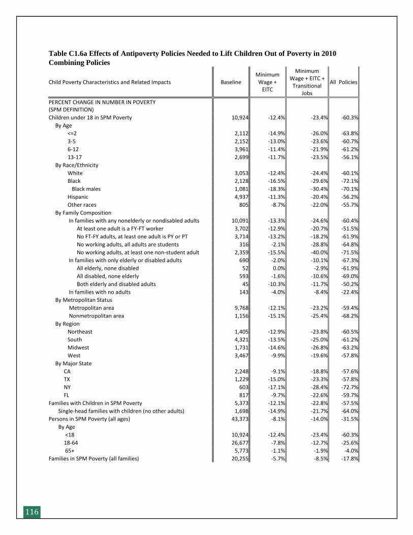
116
Table C1.6a Effects of Antipoverty Policies Needed to Lift Children Out of Poverty in 2010
Combining Policies
Child Poverty Characteristics and Related Impacts Baseline Minimum
Wage + EITC
Minimum Wage + EITC +
Transitional Jobs
All Policies
PERCENT CHANGE IN NUMBER IN POVERTY (SPM DEFINITION)
Children under 18 in SPM Poverty 10,924 -12.4% -23.4% -60.3%
By Age
<=2 2,112 -14.9% -26.0% -63.8%
3-5 2,152 -13.0% -23.6% -60.7%
6-12 3,961 -11.4% -21.9% -61.2%
13-17 2,699 -11.7% -23.5% -56.1%
By Race/Ethnicity
White 3,053 -12.4% -24.4% -60.1%
Black 2,128 -16.5% -29.6% -72.1%
Black males 1,081 -18.3% -30.4% -70.1%
Hispanic 4,937 -11.3% -20.4% -56.2%
Other races 805 -8.7% -22.0% -55.7%
By Family Composition
In families with any nonelderly or nondisabled adults 10,091 -13.3% -24.6% -60.4%
At least one adult is a FY-FT worker 3,702 -12.9% -20.7% -51.5%
No FT-FY adults, at least one adult is PY or PT 3,714 -13.2% -18.2% -61.9%
No working adults, all adults are students 316 -2.1% -28.8% -64.8%
No working adults, at least one non-student adult 2,359 -15.5% -40.0% -71.5%
In families with only elderly or disabled adults 690 -2.0% -10.1% -67.3%
All elderly, none disabled 52 0.0% -2.9% -61.9%
All disabled, none elderly 593 -1.6% -10.6% -69.0%
Both elderly and disabled adults 45 -10.3% -11.7% -50.2%
In families with no adults 143 -4.0% -8.4% -22.4%
By Metropolitan Status
Metropolitan area 9,768 -12.1% -23.2% -59.4%
Nonmetropolitan area 1,156 -15.1% -25.4% -68.2%
By Region
Northeast 1,405 -12.9% -23.8% -60.5%
South 4,321 -13.5% -25.0% -61.2%
Midwest 1,731 -14.6% -26.8% -63.2%
West 3,467 -9.9% -19.6% -57.8%
By Major State
CA 2,248 -9.1% -18.8% -57.6%
TX 1,229 -15.0% -23.3% -57.8%
NY 603 -17.1% -28.4% -72.7%
FL 817 -9.7% -22.6% -59.7%
Families with Children in SPM Poverty 5,373 -12.1% -22.8% -57.5%
Single-head families with children (no other adults) 1,698 -14.9% -21.7% -64.0%
Persons in SPM Poverty (all ages) 43,373 -8.1% -14.0% -31.5%
By Age
<18 10,924 -12.4% -23.4% -60.3%
18-64 26,677 -7.8% -12.7% -25.6%
65+ 5,773 -1.1% -1.9% -4.0%
Families in SPM Poverty (all families) 20,255 -5.7% -8.5% -17.8%
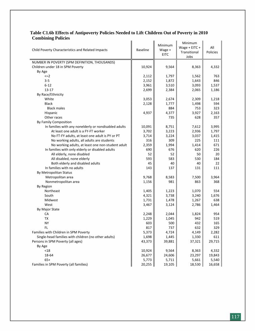
117
Table C1.6b Effects of Antipoverty Policies Needed to Lift Children Out of Poverty in 2010 Combining Policies
Child Poverty Characteristics and Related Impacts Baseline Minimum Wage +
EITC
Minimum Wage + EITC +
Transitional Jobs
All Policies
NUMBER IN POVERTY (SPM DEFINITION, THOUSANDS) Children under 18 in SPM Poverty 10,924 9,564 8,363 4,332 By Age <=2 2,112 1,797 1,562 763 3-5 2,152 1,872 1,643 846 6-12 3,961 3,510 3,093 1,537 13-17 2,699 2,384 2,065 1,186 By Race/Ethnicity White 3,053 2,674 2,309 1,218 Black 2,128 1,777 1,498 594 Black males 884 753 323 Hispanic 4,937 4,377 3,927 2,163 Other races 735 628 357 By Family Composition In families with any nonelderly or nondisabled adults 10,091 8,751 7,612 3,995 At least one adult is a FY-FT worker 3,702 3,223 2,936 1,797 No FT-FY adults, at least one adult is PY or PT 3,714 3,224 3,037 1,415 No working adults, all adults are students 316 309 225 111 No working adults, at least one non-student adult 2,359 1,994 1,414 671 In families with only elderly or disabled adults 690 676 620 226 All elderly, none disabled 52 52 50 20 All disabled, none elderly 593 583 530 184 Both elderly and disabled adults 45 40 40 22 In families with no adults 143 137 131 111 By Metropolitan Status Metropolitan area 9,768 8,583 7,500 3,964 Nonmetropolitan area 1,156 981 863 368 By Region Northeast 1,405 1,223 1,070 554 South 4,321 3,738 3,240 1,676 Midwest 1,731 1,478 1,267 638 West 3,467 3,124 2,786 1,464 By Major State CA 2,248 2,044 1,824 954 TX 1,229 1,045 942 519 NY 603 500 432 165 FL 817 737 632 329 Families with Children in SPM Poverty 5,373 4,724 4,149 2,282 Single-head families with children (no other adults) 1,698 1,445 1,330 611 Persons in SPM Poverty (all ages) 43,373 39,881 37,321 29,715 By Age <18 10,924 9,564 8,363 4,332 18-64 26,677 24,606 23,297 19,843 65+ 5,773 5,711 5,661 5,540 Families in SPM Poverty (all families) 20,255 19,105 18,530 16,658
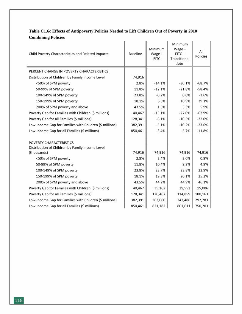
118
Table C1.6c Effects of Antipoverty Policies Needed to Lift Children Out of Poverty in 2010
Combining Policies
Child Poverty Characteristics and Related Impacts Baseline Minimum
Wage + EITC
Minimum Wage + EITC +
Transitional Jobs
All Policies
PERCENT CHANGE IN POVERTY CHARACTERISTICS
Distribution of Children by Family Income Level 74,916
<50% of SPM poverty 2.8% -14.1% -30.1% -68.7%
50-99% of SPM poverty 11.8% -12.1% -21.8% -58.4%
100-149% of SPM poverty 23.8% -0.2% 0.0% -3.6%
150-199% of SPM poverty 18.1% 6.5% 10.9% 39.1%
200% of SPM poverty and above 43.5% 1.5% 3.3% 5.9%
Poverty Gap for Families with Children ($ millions) 40,467 -13.1% -27.0% -62.9%
Poverty Gap for all Families ($ millions) 128,341 -6.1% -10.5% -22.0%
Low-Income Gap for Families with Children ($ millions) 382,391 -5.1% -10.2% -23.6%
Low-Income Gap for all Families ($ millions) 850,461 -3.4% -5.7% -11.8%
POVERTY CHARACTERISTICS Distribution of Children by Family Income Level (thousands) 74,916 74,916 74,916 74,916
<50% of SPM poverty 2.8% 2.4% 2.0% 0.9%
50-99% of SPM poverty 11.8% 10.4% 9.2% 4.9%
100-149% of SPM poverty 23.8% 23.7% 23.8% 22.9%
150-199% of SPM poverty 18.1% 19.3% 20.1% 25.2%
200% of SPM poverty and above 43.5% 44.2% 44.9% 46.1%
Poverty Gap for Families with Children ($ millions) 40,467 35,162 29,552 15,006
Poverty Gap for all Families ($ millions) 128,341 120,467 114,859 100,163
Low-Income Gap for Families with Children ($ millions) 382,391 363,060 343,486 292,283
Low-Income Gap for all Families ($ millions) 850,461 821,182 801,611 750,203
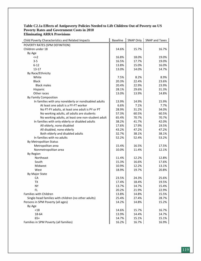
119
Table C2.1a Effects of Antipoverty Policies Needed to Lift Children Out of Poverty on US
Poverty Rates and Government Costs in 2010 Eliminating ARRA Provisions
Child Poverty Characteristics and Related Impacts Baseline SNAP Only SNAP and Taxes
POVERTY RATES (SPM DEFINITION) Children under 18 14.6% 15.7% 16.7% By Age <=2 16.8% 18.0% 19.0% 3-5 16.5% 17.7% 19.0% 6-12 13.8% 15.0% 16.0% 13-17 13.0% 14.0% 14.7% By Race/Ethnicity White 7.5% 8.2% 8.9% Black 20.3% 22.4% 23.6% Black males 20.4% 22.9% 23.9% Hispanic 28.1% 29.6% 31.3% Other races 13.0% 13.9% 14.8% By Family Composition In families with any nonelderly or nondisabled adults 13.9% 14.9% 15.9% At least one adult is a FY-FT worker 6.6% 7.1% 7.7% No FT-FY adults, at least one adult is PY or PT 28.9% 31.2% 34.0% No working adults, all adults are students 57.3% 60.5% 60.5% No working adults, at least one non-student adult 65.4% 70.7% 70.7% In families with only elderly or disabled adults 38.2% 41.7% 42.0% All elderly, none disabled 17.6% 17.9% 19.5% All disabled, none elderly 43.2% 47.2% 47.2% Both elderly and disabled adults 32.7% 38.1% 38.1% In families with no adults 52.2% 52.4% 53.2% By Metropolitan Status Metropolitan area 15.4% 16.5% 17.5% Nonmetropolitan area 10.0% 11.4% 12.1% By Region Northeast 11.4% 12.2% 12.8% South 15.3% 16.6% 17.6% Midwest 10.9% 12.2% 13.1% West 18.9% 19.7% 20.8% By Major State CA 23.5% 24.3% 25.6% TX 17.4% 18.4% 19.5% NY 13.7% 14.7% 15.4% FL 20.2% 21.9% 22.9% Families with Children 13.8% 14.8% 15.5% Single-head families with children (no other adults) 25.4% 27.4% 28.7% Persons in SPM Poverty (all ages) 14.2% 14.8% 15.2% By Age <18 14.6% 15.7% 16.7% 18-64 13.9% 14.4% 14.7% 65+ 14.7% 15.1% 15.1% Families in SPM Poverty (all families) 16.2% 16.7% 16.9%
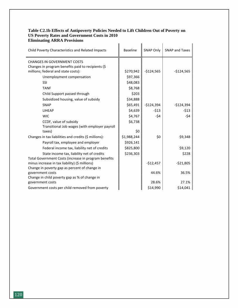
120
Table C2.1b Effects of Antipoverty Policies Needed to Lift Children Out of Poverty on
US Poverty Rates and Government Costs in 2010 Eliminating ARRA Provisions
Child Poverty Characteristics and Related Impacts Baseline SNAP Only SNAP and Taxes
CHANGES IN GOVERNMENT COSTS Changes in program benefits paid to recipients ($ millions; federal and state costs): $270,942 -$124,565 -$124,565
Unemployment compensation $97,366
SSI $48,083
TANF $8,768
Child Support passed through $203
Subsidized housing, value of subsidy $34,888
SNAP $65,491 -$124,394 -$124,394
LIHEAP $4,639 -$13 -$13
WIC $4,767 -$4 -$4
CCDF, value of subsidy $6,738
Transitional Job wages (with employer payroll taxes) $0
Changes in tax liabilities and credits ($ millions): $1,988,244 $0 $9,348
Payroll tax, employee and employer $926,141
Federal income tax, liability net of credits $825,800 $9,120
State income tax, liability net of credits $236,303 $228 Total Government Costs (increase in program benefits minus increase in tax liability) ($ millions) -$12,457 -$21,805 Change in poverty gap as percent of change in government costs 44.6% 36.5% Change in child poverty gap as % of change in government costs 28.6% 27.1%
Government costs per child removed from poverty $14,990 $14,041
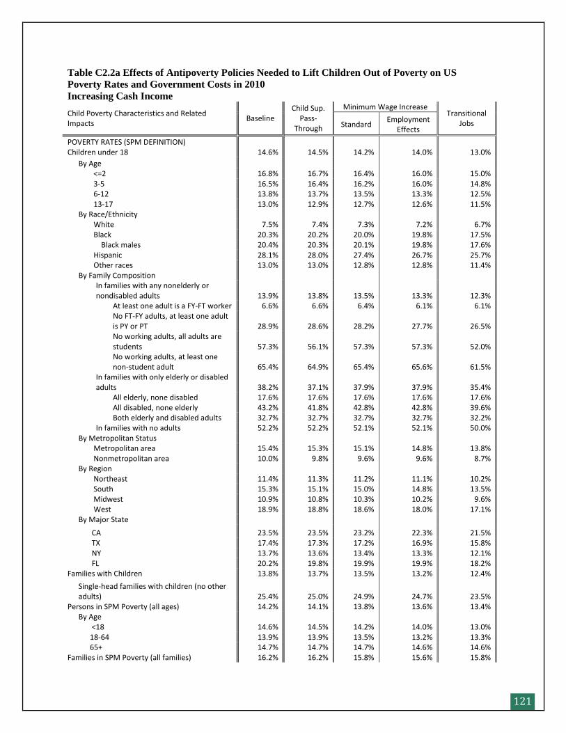
121
Table C2.2a Effects of Antipoverty Policies Needed to Lift Children Out of Poverty on US
Poverty Rates and Government Costs in 2010 Increasing Cash Income
Child Poverty Characteristics and Related Impacts
Baseline Child Sup.
Pass-Through
Minimum Wage Increase Transitional
Jobs Standard Employment
Effects
POVERTY RATES (SPM DEFINITION) Children under 18 14.6% 14.5% 14.2% 14.0% 13.0%
By Age <=2 16.8% 16.7% 16.4% 16.0% 15.0% 3-5 16.5% 16.4% 16.2% 16.0% 14.8% 6-12 13.8% 13.7% 13.5% 13.3% 12.5% 13-17 13.0% 12.9% 12.7% 12.6% 11.5% By Race/Ethnicity White 7.5% 7.4% 7.3% 7.2% 6.7% Black 20.3% 20.2% 20.0% 19.8% 17.5% Black males 20.4% 20.3% 20.1% 19.8% 17.6% Hispanic 28.1% 28.0% 27.4% 26.7% 25.7% Other races 13.0% 13.0% 12.8% 12.8% 11.4% By Family Composition
In families with any nonelderly or nondisabled adults 13.9% 13.8% 13.5% 13.3% 12.3%
At least one adult is a FY-FT worker 6.6% 6.6% 6.4% 6.1% 6.1%
No FT-FY adults, at least one adult is PY or PT 28.9% 28.6% 28.2% 27.7% 26.5%
No working adults, all adults are students 57.3% 56.1% 57.3% 57.3% 52.0%
No working adults, at least one non-student adult 65.4% 64.9% 65.4% 65.6% 61.5%
In families with only elderly or disabled adults 38.2% 37.1% 37.9% 37.9% 35.4%
All elderly, none disabled 17.6% 17.6% 17.6% 17.6% 17.6% All disabled, none elderly 43.2% 41.8% 42.8% 42.8% 39.6% Both elderly and disabled adults 32.7% 32.7% 32.7% 32.7% 32.2% In families with no adults 52.2% 52.2% 52.1% 52.1% 50.0% By Metropolitan Status Metropolitan area 15.4% 15.3% 15.1% 14.8% 13.8% Nonmetropolitan area 10.0% 9.8% 9.6% 9.6% 8.7% By Region Northeast 11.4% 11.3% 11.2% 11.1% 10.2% South 15.3% 15.1% 15.0% 14.8% 13.5% Midwest 10.9% 10.8% 10.3% 10.2% 9.6% West 18.9% 18.8% 18.6% 18.0% 17.1% By Major State
CA 23.5% 23.5% 23.2% 22.3% 21.5% TX 17.4% 17.3% 17.2% 16.9% 15.8% NY 13.7% 13.6% 13.4% 13.3% 12.1% FL 20.2% 19.8% 19.9% 19.9% 18.2% Families with Children 13.8% 13.7% 13.5% 13.2% 12.4%
Single-head families with children (no other adults) 25.4% 25.0% 24.9% 24.7% 23.5%
Persons in SPM Poverty (all ages) 14.2% 14.1% 13.8% 13.6% 13.4% By Age <18 14.6% 14.5% 14.2% 14.0% 13.0% 18-64 13.9% 13.9% 13.5% 13.2% 13.3% 65+ 14.7% 14.7% 14.7% 14.6% 14.6% Families in SPM Poverty (all families) 16.2% 16.2% 15.8% 15.6% 15.8%
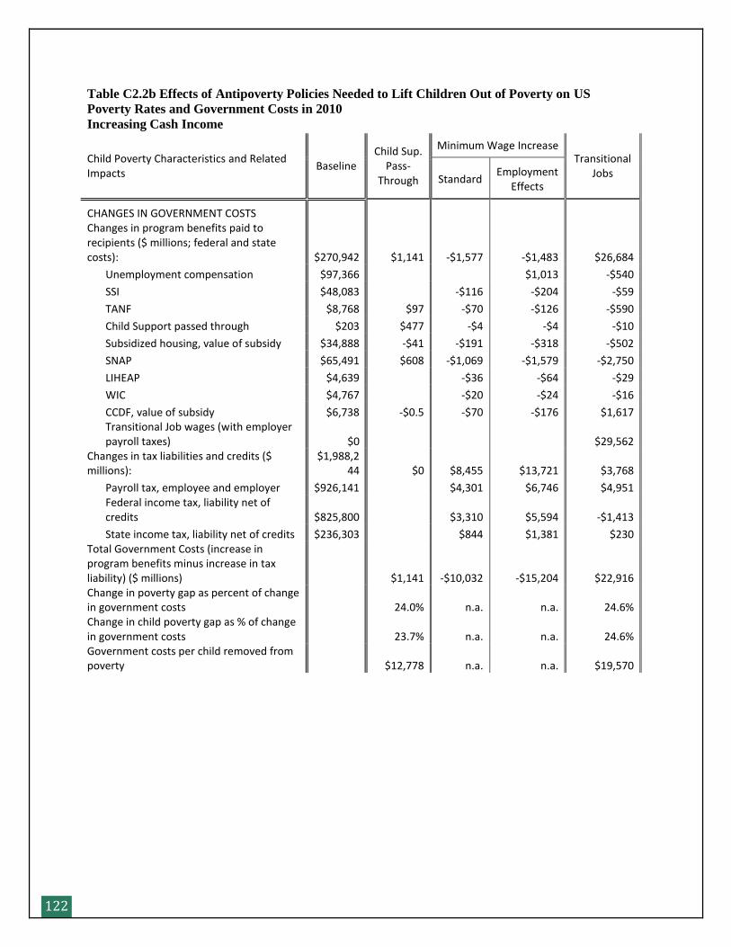
122
Table C2.2b Effects of Antipoverty Policies Needed to Lift Children Out of Poverty on US
Poverty Rates and Government Costs in 2010 Increasing Cash Income
Child Poverty Characteristics and Related Impacts
Baseline Child Sup.
Pass-Through
Minimum Wage Increase Transitional
Jobs Standard Employment
Effects
CHANGES IN GOVERNMENT COSTS Changes in program benefits paid to recipients ($ millions; federal and state costs): $270,942 $1,141 -$1,577 -$1,483 $26,684
Unemployment compensation $97,366 $1,013 -$540
SSI $48,083 -$116 -$204 -$59
TANF $8,768 $97 -$70 -$126 -$590
Child Support passed through $203 $477 -$4 -$4 -$10
Subsidized housing, value of subsidy $34,888 -$41 -$191 -$318 -$502
SNAP $65,491 $608 -$1,069 -$1,579 -$2,750
LIHEAP $4,639 -$36 -$64 -$29
WIC $4,767 -$20 -$24 -$16
CCDF, value of subsidy $6,738 -$0.5 -$70 -$176 $1,617
Transitional Job wages (with employer payroll taxes) $0 $29,562
Changes in tax liabilities and credits ($ millions):
$1,988,244 $0 $8,455 $13,721 $3,768
Payroll tax, employee and employer $926,141 $4,301 $6,746 $4,951
Federal income tax, liability net of credits $825,800 $3,310 $5,594 -$1,413
State income tax, liability net of credits $236,303 $844 $1,381 $230 Total Government Costs (increase in program benefits minus increase in tax liability) ($ millions) $1,141 -$10,032 -$15,204 $22,916 Change in poverty gap as percent of change in government costs 24.0% n.a. n.a. 24.6% Change in child poverty gap as % of change in government costs 23.7% n.a. n.a. 24.6% Government costs per child removed from poverty $12,778 n.a. n.a. $19,570

123
Table C2.3a Effects of Antipoverty Policies Needed to Lift Children Out of Poverty on US
Poverty Rates and Government Costs in 2010 Increasing In-Kind Income
Child Poverty Characteristics and Related Impacts Baseline Increased Housing
Vouchers
SNAP Benefit Increase
All Families
Families with Children
POVERTY RATES (SPM DEFINITION) Children under 18 14.6% 11.5% 12.2% 12.2% By Age <=2 16.8% 12.9% 14.1% 14.1% 3-5 16.5% 13.0% 13.4% 13.4% 6-12 13.8% 11.1% 11.5% 11.5% 13-17 13.0% 10.5% 11.2% 11.2% By Race/Ethnicity White 7.5% 6.4% 5.9% 6.0% Black 20.3% 15.3% 16.2% 16.3% Black males 20.4% 15.6% 16.5% 16.7% Hispanic 28.1% 21.8% 24.6% 24.6% Other races 13.0% 10.1% 11.3% 11.3% By Family Composition
In families with any nonelderly or nondisabled adults 13.9% 11.0% 11.6% 11.6%
At least one adult is a FY-FT worker 6.6% 5.5% 5.6% 5.6%
No FT-FY adults, at least one adult is PY or PT 28.9% 22.0% 23.9% 24.0% No working adults, all adults are students 57.3% 43.9% 46.5% 46.5%
No working adults, at least one non-student adult 65.4% 53.5% 55.0% 55.7%
In families with only elderly or disabled adults 38.2% 26.4% 30.0% 30.0% All elderly, none disabled 17.6% 13.5% 15.0% 15.0% All disabled, none elderly 43.2% 28.9% 33.7% 33.7% Both elderly and disabled adults 32.7% 29.0% 25.1% 25.1% In families with no adults 52.2% 46.1% 49.2% 49.2%
By Metropolitan Status Metropolitan area 15.4% 12.1% 13.1% 13.1% Nonmetropolitan area 10.0% 8.3% 7.2% 7.2% By Region Northeast 11.4% 8.3% 9.7% 9.7% South 15.3% 12.8% 12.3% 12.4% Midwest 10.9% 9.4% 8.5% 8.6% West 18.9% 13.6% 16.8% 16.8% By Major State CA 23.5% 16.4% 21.7% 21.7%
TX 17.4% 14.3% 15.1% 15.1% NY 13.7% 8.5% 11.5% 11.5% FL 20.2% 16.3% 17.0% 17.4% Families with Children 13.8% 11.1% 11.7% 11.7% Single-head families with children (no other adults) 25.4% 19.6% 21.2% 21.2% Persons in SPM Poverty (all ages) 14.2% 12.8% 12.7% 13.1% By Age <18 14.6% 11.5% 12.2% 12.2% 18-64 13.9% 12.9% 12.7% 13.1% 65+ 14.7% 14.6% 13.9% 14.6% Families in SPM Poverty (all families) 16.2% 15.4% 15.0% 15.6%
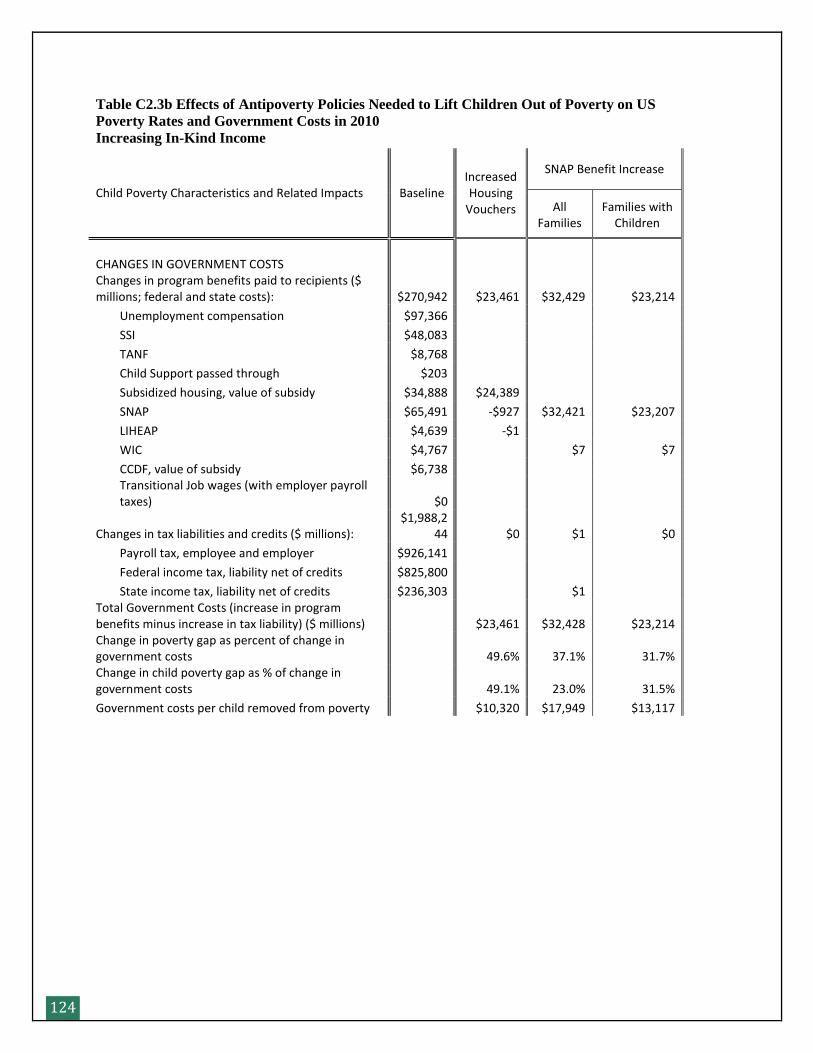
124
Table C2.3b Effects of Antipoverty Policies Needed to Lift Children Out of Poverty on US
Poverty Rates and Government Costs in 2010 Increasing In-Kind Income
Child Poverty Characteristics and Related Impacts Baseline Increased Housing
Vouchers
SNAP Benefit Increase
All Families
Families with Children
CHANGES IN GOVERNMENT COSTS Changes in program benefits paid to recipients ($ millions; federal and state costs): $270,942 $23,461 $32,429 $23,214
Unemployment compensation $97,366
SSI $48,083
TANF $8,768
Child Support passed through $203
Subsidized housing, value of subsidy $34,888 $24,389
SNAP $65,491 -$927 $32,421 $23,207
LIHEAP $4,639 -$1
WIC $4,767 $7 $7
CCDF, value of subsidy $6,738
Transitional Job wages (with employer payroll taxes) $0
Changes in tax liabilities and credits ($ millions): $1,988,2
44 $0 $1 $0
Payroll tax, employee and employer $926,141
Federal income tax, liability net of credits $825,800
State income tax, liability net of credits $236,303 $1 Total Government Costs (increase in program benefits minus increase in tax liability) ($ millions) $23,461 $32,428 $23,214 Change in poverty gap as percent of change in government costs 49.6% 37.1% 31.7% Change in child poverty gap as % of change in government costs 49.1% 23.0% 31.5%
Government costs per child removed from poverty $10,320 $17,949 $13,117
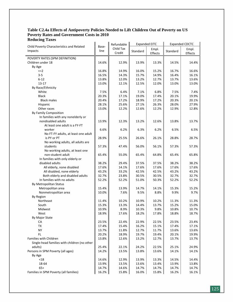
125
Table C2.4a Effects of Antipoverty Policies Needed to Lift Children Out of Poverty on US
Poverty Rates and Government Costs in 2010 Reducing Taxes
Child Poverty Characteristics and Related Impacts
Base-line
Refundable Child Tax
Credit
Expanded EITC Expanded CDCTC
Standard Empl.
Effects Standard
Empl. Effects
POVERTY RATES (SPM DEFINITION) Children under 18 14.6% 12.9% 13.9% 13.3% 14.5% 14.4% By Age <=2 16.8% 14.9% 16.0% 15.2% 16.7% 16.6% 3-5 16.5% 14.3% 15.7% 14.9% 16.4% 16.1% 6-12 13.8% 12.0% 13.2% 12.7% 13.7% 13.6% 13-17 13.0% 12.1% 12.5% 12.0% 13.0% 13.0% By Race/Ethnicity White 7.5% 6.4% 7.1% 6.8% 7.5% 7.4% Black 20.3% 17.1% 19.0% 17.4% 20.1% 19.9% Black males 20.4% 17.2% 18.9% 17.2% 20.3% 20.1% Hispanic 28.1% 25.6% 27.1% 26.3% 28.0% 27.9% Other races 13.0% 12.2% 12.6% 12.2% 12.9% 12.8% By Family Composition
In families with any nonelderly or nondisabled adults 13.9% 12.3% 13.2% 12.6% 13.8% 13.7%
At least one adult is a FY-FT worker 6.6% 6.2% 6.3% 6.2% 6.5% 6.5%
No FT-FY adults, at least one adult is PY or PT 28.9% 25.5% 26.6% 26.1% 28.8% 28.7%
No working adults, all adults are students 57.3% 47.4% 56.0% 56.1% 57.3% 57.3%
No working adults, at least one non-student adult 65.4% 55.0% 65.4% 64.8% 65.4% 65.8%
In families with only elderly or disabled adults 38.2% 29.4% 37.5% 37.5% 38.2% 38.2%
All elderly, none disabled 17.6% 14.1% 17.6% 17.6% 17.6% 17.6% All disabled, none elderly 43.2% 33.2% 42.5% 42.5% 43.2% 43.2% Both elderly and disabled adults 32.7% 23.8% 30.5% 30.5% 32.7% 32.7% In families with no adults 52.2% 52.2% 51.0% 50.3% 52.2% 52.2% By Metropolitan Status Metropolitan area 15.4% 13.9% 14.7% 14.1% 15.3% 15.2% Nonmetropolitan area 10.0% 7.6% 9.5% 8.8% 9.9% 9.7% By Region Northeast 11.4% 10.2% 10.9% 10.2% 11.3% 11.3% South 15.3% 13.3% 14.4% 13.7% 15.2% 15.0% Midwest 10.9% 8.9% 10.3% 9.8% 10.8% 10.7% West 18.9% 17.6% 18.2% 17.8% 18.8% 18.7% By Major State CA 23.5% 22.4% 22.9% 22.5% 23.5% 23.4% TX 17.4% 15.4% 16.2% 15.1% 17.4% 17.1% NY 13.7% 11.8% 12.7% 11.7% 13.6% 13.6% FL 20.2% 18.9% 19.7% 19.4% 20.1% 19.9% Families with Children 13.8% 12.6% 13.2% 12.7% 13.7% 13.7%
Single-head families with children (no other adults) 25.4% 22.1% 24.2% 22.5% 25.1% 24.9%
Persons in SPM Poverty (all ages) 14.2% 13.5% 13.8% 13.6% 14.1% 14.1% By Age <18 14.6% 12.9% 13.9% 13.3% 14.5% 14.4% 18-64 13.9% 13.5% 13.6% 13.4% 13.9% 13.8% 65+ 14.7% 14.6% 14.7% 14.7% 14.7% 14.7% Families in SPM Poverty (all families) 16.2% 15.8% 16.0% 15.8% 16.2% 16.1%
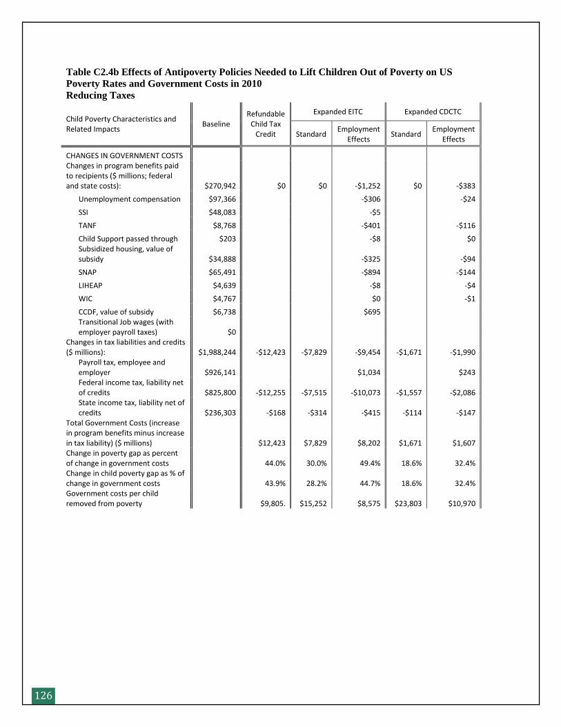
126
Table C2.4b Effects of Antipoverty Policies Needed to Lift Children Out of Poverty on US
Poverty Rates and Government Costs in 2010 Reducing Taxes
Child Poverty Characteristics and Related Impacts
Baseline Refundable
Child Tax Credit
Expanded EITC Expanded CDCTC
Standard Employment
Effects Standard
Employment Effects
CHANGES IN GOVERNMENT COSTS Changes in program benefits paid to recipients ($ millions; federal and state costs): $270,942 $0 $0 -$1,252 $0 -$383
Unemployment compensation $97,366 -$306 -$24
SSI $48,083 -$5
TANF $8,768 -$401 -$116
Child Support passed through $203 -$8 $0
Subsidized housing, value of subsidy $34,888 -$325 -$94
SNAP $65,491 -$894 -$144
LIHEAP $4,639 -$8 -$4
WIC $4,767 $0 -$1
CCDF, value of subsidy $6,738 $695
Transitional Job wages (with employer payroll taxes) $0
Changes in tax liabilities and credits ($ millions): $1,988,244 -$12,423 -$7,829 -$9,454 -$1,671 -$1,990
Payroll tax, employee and employer $926,141 $1,034 $243
Federal income tax, liability net of credits $825,800 -$12,255 -$7,515 -$10,073 -$1,557 -$2,086
State income tax, liability net of credits $236,303 -$168 -$314 -$415 -$114 -$147
Total Government Costs (increase in program benefits minus increase in tax liability) ($ millions) $12,423 $7,829 $8,202 $1,671 $1,607 Change in poverty gap as percent of change in government costs 44.0% 30.0% 49.4% 18.6% 32.4% Change in child poverty gap as % of change in government costs 43.9% 28.2% 44.7% 18.6% 32.4% Government costs per child removed from poverty $9,805. $15,252 $8,575 $23,803 $10,970
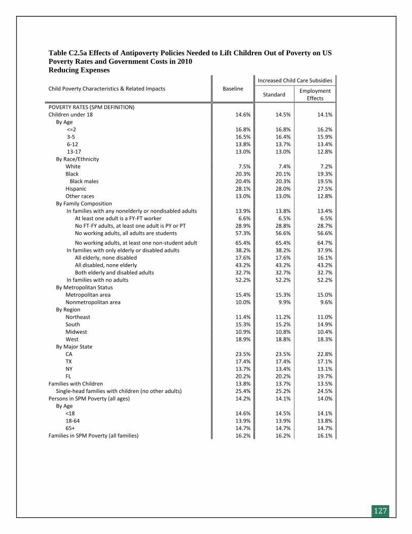
127
Table C2.5a Effects of Antipoverty Policies Needed to Lift Children Out of Poverty on US
Poverty Rates and Government Costs in 2010 Reducing Expenses
Child Poverty Characteristics & Related Impacts Baseline
Increased Child Care Subsidies
Standard Employment
Effects
POVERTY RATES (SPM DEFINITION) Children under 18 14.6% 14.5% 14.1% By Age <=2 16.8% 16.8% 16.2% 3-5 16.5% 16.4% 15.9% 6-12 13.8% 13.7% 13.4% 13-17 13.0% 13.0% 12.8% By Race/Ethnicity White 7.5% 7.4% 7.2% Black 20.3% 20.1% 19.3% Black males 20.4% 20.3% 19.5% Hispanic 28.1% 28.0% 27.5% Other races 13.0% 13.0% 12.8% By Family Composition In families with any nonelderly or nondisabled adults 13.9% 13.8% 13.4% At least one adult is a FY-FT worker 6.6% 6.5% 6.5% No FT-FY adults, at least one adult is PY or PT 28.9% 28.8% 28.7% No working adults, all adults are students 57.3% 56.6% 56.6%
No working adults, at least one non-student adult 65.4% 65.4% 64.7% In families with only elderly or disabled adults 38.2% 38.2% 37.9% All elderly, none disabled 17.6% 17.6% 16.1% All disabled, none elderly 43.2% 43.2% 43.2% Both elderly and disabled adults 32.7% 32.7% 32.7% In families with no adults 52.2% 52.2% 52.2% By Metropolitan Status Metropolitan area 15.4% 15.3% 15.0% Nonmetropolitan area 10.0% 9.9% 9.6% By Region Northeast 11.4% 11.2% 11.0% South 15.3% 15.2% 14.9% Midwest 10.9% 10.8% 10.4% West 18.9% 18.8% 18.3% By Major State CA 23.5% 23.5% 22.8% TX 17.4% 17.4% 17.1% NY 13.7% 13.4% 13.1% FL 20.2% 20.2% 19.7% Families with Children 13.8% 13.7% 13.5% Single-head families with children (no other adults) 25.4% 25.2% 24.5% Persons in SPM Poverty (all ages) 14.2% 14.1% 14.0% By Age <18 14.6% 14.5% 14.1% 18-64 13.9% 13.9% 13.8% 65+ 14.7% 14.7% 14.7% Families in SPM Poverty (all families) 16.2% 16.2% 16.1%
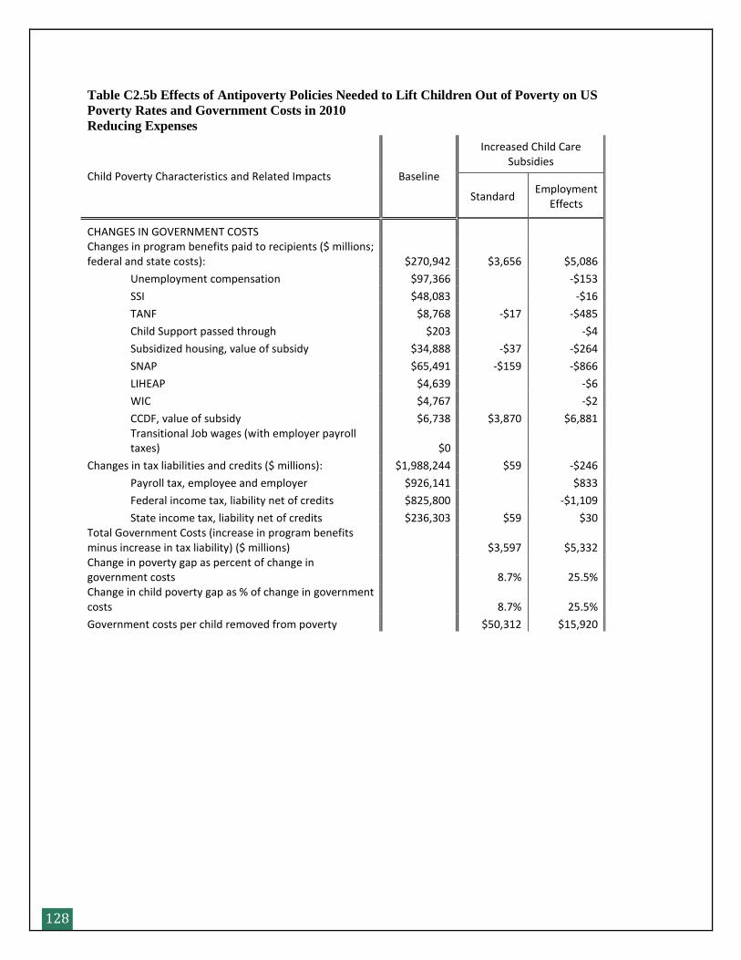
128
Table C2.5b Effects of Antipoverty Policies Needed to Lift Children Out of Poverty on US
Poverty Rates and Government Costs in 2010 Reducing Expenses
Child Poverty Characteristics and Related Impacts Baseline
Increased Child Care Subsidies
Standard Employment
Effects
CHANGES IN GOVERNMENT COSTS Changes in program benefits paid to recipients ($ millions; federal and state costs): $270,942 $3,656 $5,086
Unemployment compensation $97,366 -$153
SSI $48,083 -$16
TANF $8,768 -$17 -$485
Child Support passed through $203 -$4
Subsidized housing, value of subsidy $34,888 -$37 -$264
SNAP $65,491 -$159 -$866
LIHEAP $4,639 -$6
WIC $4,767 -$2
CCDF, value of subsidy $6,738 $3,870 $6,881
Transitional Job wages (with employer payroll taxes) $0
Changes in tax liabilities and credits ($ millions): $1,988,244 $59 -$246
Payroll tax, employee and employer $926,141 $833
Federal income tax, liability net of credits $825,800 -$1,109
State income tax, liability net of credits $236,303 $59 $30 Total Government Costs (increase in program benefits minus increase in tax liability) ($ millions) $3,597 $5,332 Change in poverty gap as percent of change in government costs 8.7% 25.5% Change in child poverty gap as % of change in government costs 8.7% 25.5%
Government costs per child removed from poverty $50,312 $15,920
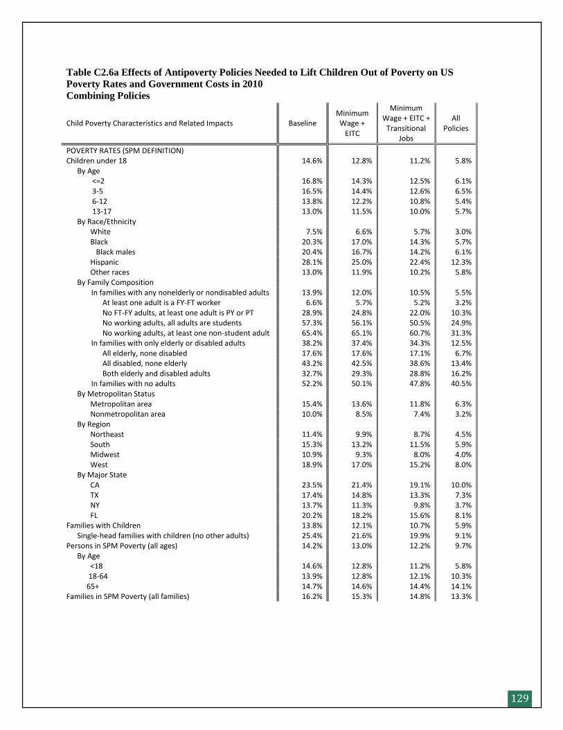
129
Table C2.6a Effects of Antipoverty Policies Needed to Lift Children Out of Poverty on US
Poverty Rates and Government Costs in 2010 Combining Policies
Child Poverty Characteristics and Related Impacts Baseline Minimum Wage +
EITC
Minimum Wage + EITC +
Transitional Jobs
All Policies
POVERTY RATES (SPM DEFINITION) Children under 18 14.6% 12.8% 11.2% 5.8% By Age <=2 16.8% 14.3% 12.5% 6.1% 3-5 16.5% 14.4% 12.6% 6.5% 6-12 13.8% 12.2% 10.8% 5.4% 13-17 13.0% 11.5% 10.0% 5.7% By Race/Ethnicity White 7.5% 6.6% 5.7% 3.0% Black 20.3% 17.0% 14.3% 5.7% Black males 20.4% 16.7% 14.2% 6.1% Hispanic 28.1% 25.0% 22.4% 12.3% Other races 13.0% 11.9% 10.2% 5.8% By Family Composition In families with any nonelderly or nondisabled adults 13.9% 12.0% 10.5% 5.5% At least one adult is a FY-FT worker 6.6% 5.7% 5.2% 3.2% No FT-FY adults, at least one adult is PY or PT 28.9% 24.8% 22.0% 10.3% No working adults, all adults are students 57.3% 56.1% 50.5% 24.9% No working adults, at least one non-student adult 65.4% 65.1% 60.7% 31.3% In families with only elderly or disabled adults 38.2% 37.4% 34.3% 12.5% All elderly, none disabled 17.6% 17.6% 17.1% 6.7% All disabled, none elderly 43.2% 42.5% 38.6% 13.4% Both elderly and disabled adults 32.7% 29.3% 28.8% 16.2% In families with no adults 52.2% 50.1% 47.8% 40.5% By Metropolitan Status Metropolitan area 15.4% 13.6% 11.8% 6.3% Nonmetropolitan area 10.0% 8.5% 7.4% 3.2% By Region Northeast 11.4% 9.9% 8.7% 4.5% South 15.3% 13.2% 11.5% 5.9% Midwest 10.9% 9.3% 8.0% 4.0% West 18.9% 17.0% 15.2% 8.0% By Major State CA 23.5% 21.4% 19.1% 10.0% TX 17.4% 14.8% 13.3% 7.3% NY 13.7% 11.3% 9.8% 3.7% FL 20.2% 18.2% 15.6% 8.1% Families with Children 13.8% 12.1% 10.7% 5.9% Single-head families with children (no other adults) 25.4% 21.6% 19.9% 9.1% Persons in SPM Poverty (all ages) 14.2% 13.0% 12.2% 9.7% By Age <18 14.6% 12.8% 11.2% 5.8% 18-64 13.9% 12.8% 12.1% 10.3% 65+ 14.7% 14.6% 14.4% 14.1% Families in SPM Poverty (all families) 16.2% 15.3% 14.8% 13.3%
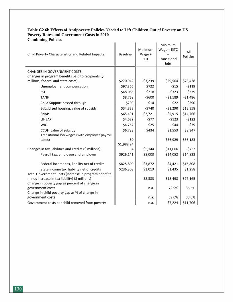
130
Table C2.6b Effects of Antipoverty Policies Needed to Lift Children Out of Poverty on US
Poverty Rates and Government Costs in 2010 Combining Policies
Child Poverty Characteristics and Related Impacts Baseline Minimum
Wage + EITC
Minimum Wage + EITC
+ Transitional
Jobs
All Policies
CHANGES IN GOVERNMENT COSTS Changes in program benefits paid to recipients ($ millions; federal and state costs): $270,942 -$3,239 $29,564 $76,438
Unemployment compensation $97,366 $722 -$15 -$119
SSI $48,083 -$218 -$323 -$339
TANF $8,768 -$600 -$1,189 -$1,486
Child Support passed through $203 -$14 -$22 $390
Subsidized housing, value of subsidy $34,888 -$740 -$1,290 $18,858
SNAP $65,491 -$2,721 -$5,915 $14,766
LIHEAP $4,639 -$77 -$123 -$122
WIC $4,767 -$25 -$44 -$39
CCDF, value of subsidy $6,738 $434 $1,553 $8,347
Transitional Job wages (with employer payroll taxes) $0 $36,929 $36,183
Changes in tax liabilities and credits ($ millions): $1,988,24
4 $5,144 $11,066 -$727
Payroll tax, employee and employer $926,141 $8,003 $14,052 $14,823
Federal income tax, liability net of credits $825,800 -$3,872 -$4,421 -
$16,808
State income tax, liability net of credits $236,303 $1,013 $1,435 $1,258 Total Government Costs (increase in program benefits minus increase in tax liability) ($ millions) -$8,383 $18,498 $77,165 Change in poverty gap as percent of change in government costs n.a. 72.9% 36.5% Change in child poverty gap as % of change in government costs n.a. 59.0% 33.0%
Government costs per child removed from poverty n.a. $7,224 $11,706
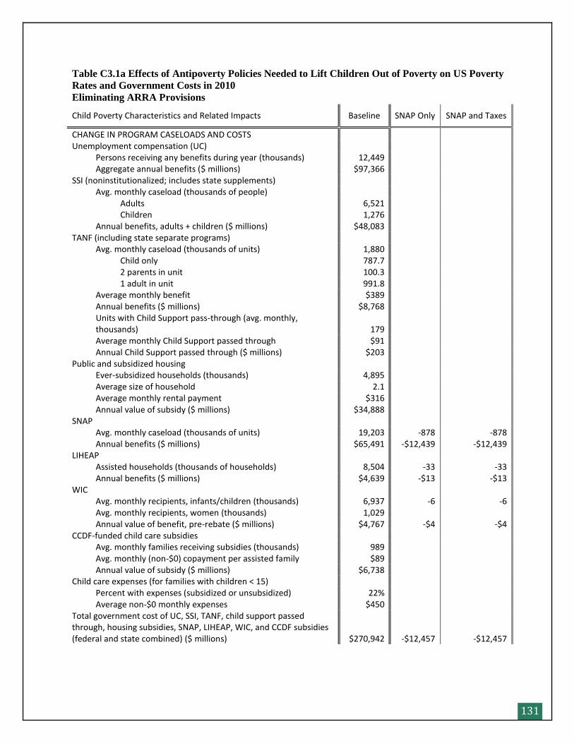
131
Table C3.1a Effects of Antipoverty Policies Needed to Lift Children Out of Poverty on US Poverty
Rates and Government Costs in 2010 Eliminating ARRA Provisions
Child Poverty Characteristics and Related Impacts Baseline SNAP Only SNAP and Taxes
CHANGE IN PROGRAM CASELOADS AND COSTS Unemployment compensation (UC) Persons receiving any benefits during year (thousands) 12,449 Aggregate annual benefits ($ millions) $97,366 SSI (noninstitutionalized; includes state supplements) Avg. monthly caseload (thousands of people) Adults 6,521 Children 1,276 Annual benefits, adults + children ($ millions) $48,083 TANF (including state separate programs) Avg. monthly caseload (thousands of units) 1,880 Child only 787.7 2 parents in unit 100.3 1 adult in unit 991.8 Average monthly benefit $389 Annual benefits ($ millions) $8,768
Units with Child Support pass-through (avg. monthly, thousands) 179
Average monthly Child Support passed through $91 Annual Child Support passed through ($ millions) $203 Public and subsidized housing Ever-subsidized households (thousands) 4,895 Average size of household 2.1 Average monthly rental payment $316 Annual value of subsidy ($ millions) $34,888 SNAP Avg. monthly caseload (thousands of units) 19,203 -878 -878 Annual benefits ($ millions) $65,491 -$12,439 -$12,439 LIHEAP Assisted households (thousands of households) 8,504 -33 -33 Annual benefits ($ millions) $4,639 -$13 -$13 WIC Avg. monthly recipients, infants/children (thousands) 6,937 -6 -6 Avg. monthly recipients, women (thousands) 1,029 Annual value of benefit, pre-rebate ($ millions) $4,767 -$4 -$4 CCDF-funded child care subsidies Avg. monthly families receiving subsidies (thousands) 989 Avg. monthly (non-$0) copayment per assisted family $89 Annual value of subsidy ($ millions) $6,738 Child care expenses (for families with children < 15) Percent with expenses (subsidized or unsubsidized) 22% Average non-$0 monthly expenses $450 Total government cost of UC, SSI, TANF, child support passed through, housing subsidies, SNAP, LIHEAP, WIC, and CCDF subsidies (federal and state combined) ($ millions) $270,942 -$12,457 -$12,457
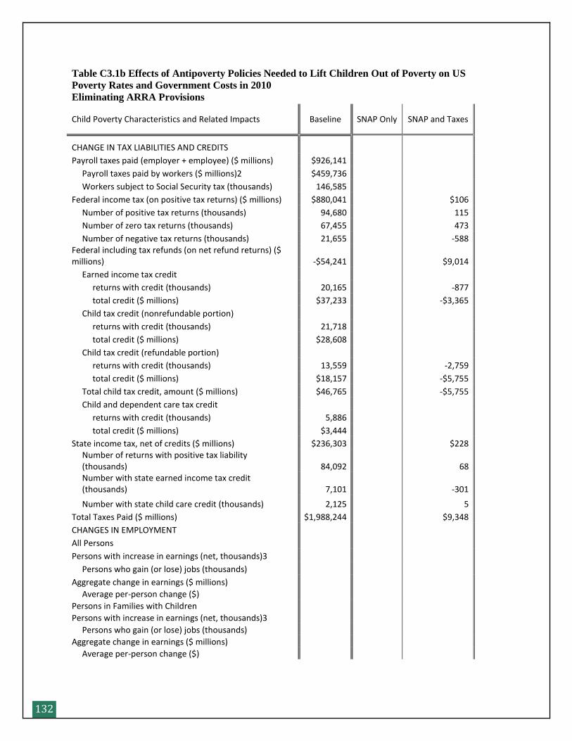
132
Table C3.1b Effects of Antipoverty Policies Needed to Lift Children Out of Poverty on US
Poverty Rates and Government Costs in 2010 Eliminating ARRA Provisions
Child Poverty Characteristics and Related Impacts Baseline SNAP Only SNAP and Taxes
CHANGE IN TAX LIABILITIES AND CREDITS
Payroll taxes paid (employer + employee) ($ millions) $926,141
Payroll taxes paid by workers ($ millions)2 $459,736
Workers subject to Social Security tax (thousands) 146,585
Federal income tax (on positive tax returns) ($ millions) $880,041 $106
Number of positive tax returns (thousands) 94,680 115
Number of zero tax returns (thousands) 67,455 473
Number of negative tax returns (thousands) 21,655 -588 Federal including tax refunds (on net refund returns) ($ millions) -$54,241 $9,014
Earned income tax credit
returns with credit (thousands) 20,165 -877
total credit ($ millions) $37,233 -$3,365
Child tax credit (nonrefundable portion)
returns with credit (thousands) 21,718
total credit ($ millions) $28,608
Child tax credit (refundable portion)
returns with credit (thousands) 13,559 -2,759
total credit ($ millions) $18,157 -$5,755
Total child tax credit, amount ($ millions) $46,765 -$5,755
Child and dependent care tax credit
returns with credit (thousands) 5,886
total credit ($ millions) $3,444
State income tax, net of credits ($ millions) $236,303 $228
Number of returns with positive tax liability (thousands) 84,092 68
Number with state earned income tax credit (thousands) 7,101 -301
Number with state child care credit (thousands) 2,125 5
Total Taxes Paid ($ millions) $1,988,244 $9,348
CHANGES IN EMPLOYMENT
All Persons
Persons with increase in earnings (net, thousands)3
Persons who gain (or lose) jobs (thousands)
Aggregate change in earnings ($ millions)
Average per-person change ($)
Persons in Families with Children
Persons with increase in earnings (net, thousands)3
Persons who gain (or lose) jobs (thousands)
Aggregate change in earnings ($ millions)
Average per-person change ($)
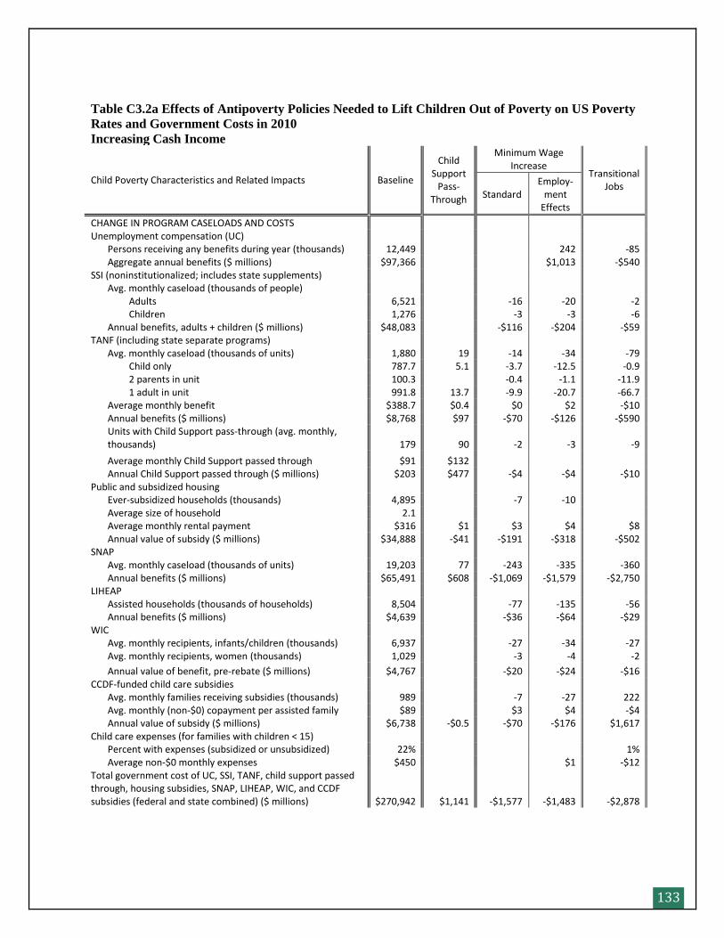
133
Table C3.2a Effects of Antipoverty Policies Needed to Lift Children Out of Poverty on US Poverty
Rates and Government Costs in 2010 Increasing Cash Income
Child Poverty Characteristics and Related Impacts Baseline
Child Support
Pass-Through
Minimum Wage Increase
Transitional Jobs
Standard Employ-
ment Effects
CHANGE IN PROGRAM CASELOADS AND COSTS Unemployment compensation (UC) Persons receiving any benefits during year (thousands) 12,449 242 -85 Aggregate annual benefits ($ millions) $97,366 $1,013 -$540 SSI (noninstitutionalized; includes state supplements) Avg. monthly caseload (thousands of people) Adults 6,521 -16 -20 -2 Children 1,276 -3 -3 -6 Annual benefits, adults + children ($ millions) $48,083 -$116 -$204 -$59 TANF (including state separate programs) Avg. monthly caseload (thousands of units) 1,880 19 -14 -34 -79 Child only 787.7 5.1 -3.7 -12.5 -0.9 2 parents in unit 100.3 -0.4 -1.1 -11.9 1 adult in unit 991.8 13.7 -9.9 -20.7 -66.7 Average monthly benefit $388.7 $0.4 $0 $2 -$10 Annual benefits ($ millions) $8,768 $97 -$70 -$126 -$590
Units with Child Support pass-through (avg. monthly, thousands) 179 90 -2 -3 -9
Average monthly Child Support passed through $91 $132 Annual Child Support passed through ($ millions) $203 $477 -$4 -$4 -$10 Public and subsidized housing Ever-subsidized households (thousands) 4,895 -7 -10 Average size of household 2.1 Average monthly rental payment $316 $1 $3 $4 $8 Annual value of subsidy ($ millions) $34,888 -$41 -$191 -$318 -$502 SNAP Avg. monthly caseload (thousands of units) 19,203 77 -243 -335 -360 Annual benefits ($ millions) $65,491 $608 -$1,069 -$1,579 -$2,750 LIHEAP Assisted households (thousands of households) 8,504 -77 -135 -56 Annual benefits ($ millions) $4,639 -$36 -$64 -$29 WIC Avg. monthly recipients, infants/children (thousands) 6,937 -27 -34 -27 Avg. monthly recipients, women (thousands) 1,029 -3 -4 -2
Annual value of benefit, pre-rebate ($ millions) $4,767 -$20 -$24 -$16 CCDF-funded child care subsidies Avg. monthly families receiving subsidies (thousands) 989 -7 -27 222 Avg. monthly (non-$0) copayment per assisted family $89 $3 $4 -$4 Annual value of subsidy ($ millions) $6,738 -$0.5 -$70 -$176 $1,617 Child care expenses (for families with children < 15) Percent with expenses (subsidized or unsubsidized) 22% 1% Average non-$0 monthly expenses $450 $1 -$12 Total government cost of UC, SSI, TANF, child support passed through, housing subsidies, SNAP, LIHEAP, WIC, and CCDF subsidies (federal and state combined) ($ millions) $270,942 $1,141 -$1,577 -$1,483 -$2,878
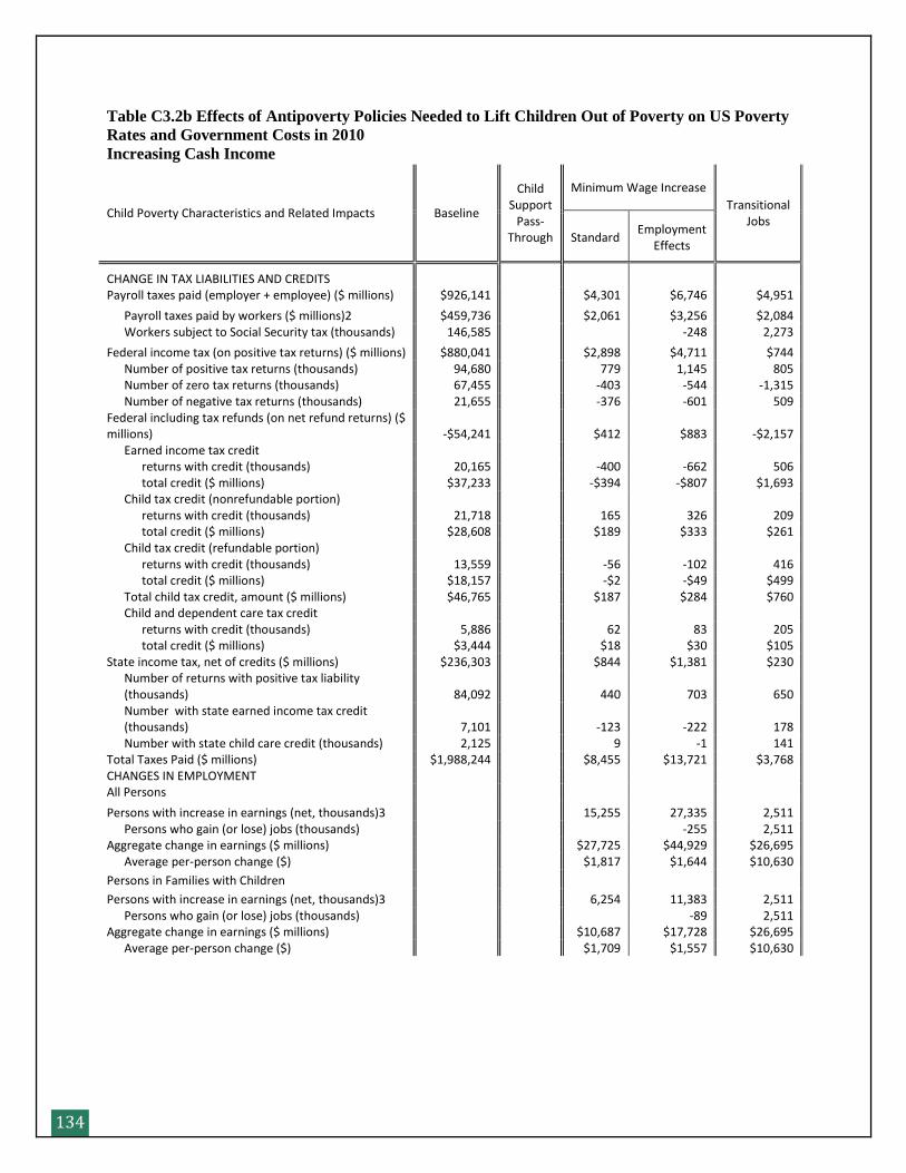
134
Table C3.2b Effects of Antipoverty Policies Needed to Lift Children Out of Poverty on US Poverty
Rates and Government Costs in 2010 Increasing Cash Income
Child Poverty Characteristics and Related Impacts Baseline
Child Support
Pass-Through
Minimum Wage Increase
Transitional Jobs
Standard Employment
Effects
CHANGE IN TAX LIABILITIES AND CREDITS Payroll taxes paid (employer + employee) ($ millions) $926,141 $4,301 $6,746 $4,951
Payroll taxes paid by workers ($ millions)2 $459,736 $2,061 $3,256 $2,084 Workers subject to Social Security tax (thousands) 146,585 -248 2,273
Federal income tax (on positive tax returns) ($ millions) $880,041 $2,898 $4,711 $744 Number of positive tax returns (thousands) 94,680 779 1,145 805 Number of zero tax returns (thousands) 67,455 -403 -544 -1,315 Number of negative tax returns (thousands) 21,655 -376 -601 509 Federal including tax refunds (on net refund returns) ($ millions) -$54,241 $412 $883 -$2,157 Earned income tax credit returns with credit (thousands) 20,165 -400 -662 506 total credit ($ millions) $37,233 -$394 -$807 $1,693 Child tax credit (nonrefundable portion) returns with credit (thousands) 21,718 165 326 209 total credit ($ millions) $28,608 $189 $333 $261 Child tax credit (refundable portion) returns with credit (thousands) 13,559 -56 -102 416 total credit ($ millions) $18,157 -$2 -$49 $499 Total child tax credit, amount ($ millions) $46,765 $187 $284 $760 Child and dependent care tax credit returns with credit (thousands) 5,886 62 83 205 total credit ($ millions) $3,444 $18 $30 $105 State income tax, net of credits ($ millions) $236,303 $844 $1,381 $230
Number of returns with positive tax liability (thousands) 84,092 440 703 650
Number with state earned income tax credit (thousands) 7,101 -123 -222 178
Number with state child care credit (thousands) 2,125 9 -1 141 Total Taxes Paid ($ millions) $1,988,244 $8,455 $13,721 $3,768 CHANGES IN EMPLOYMENT All Persons
Persons with increase in earnings (net, thousands)3 15,255 27,335 2,511 Persons who gain (or lose) jobs (thousands) -255 2,511 Aggregate change in earnings ($ millions) $27,725 $44,929 $26,695 Average per-person change ($) $1,817 $1,644 $10,630
Persons in Families with Children
Persons with increase in earnings (net, thousands)3 6,254 11,383 2,511 Persons who gain (or lose) jobs (thousands) -89 2,511 Aggregate change in earnings ($ millions) $10,687 $17,728 $26,695 Average per-person change ($) $1,709 $1,557 $10,630
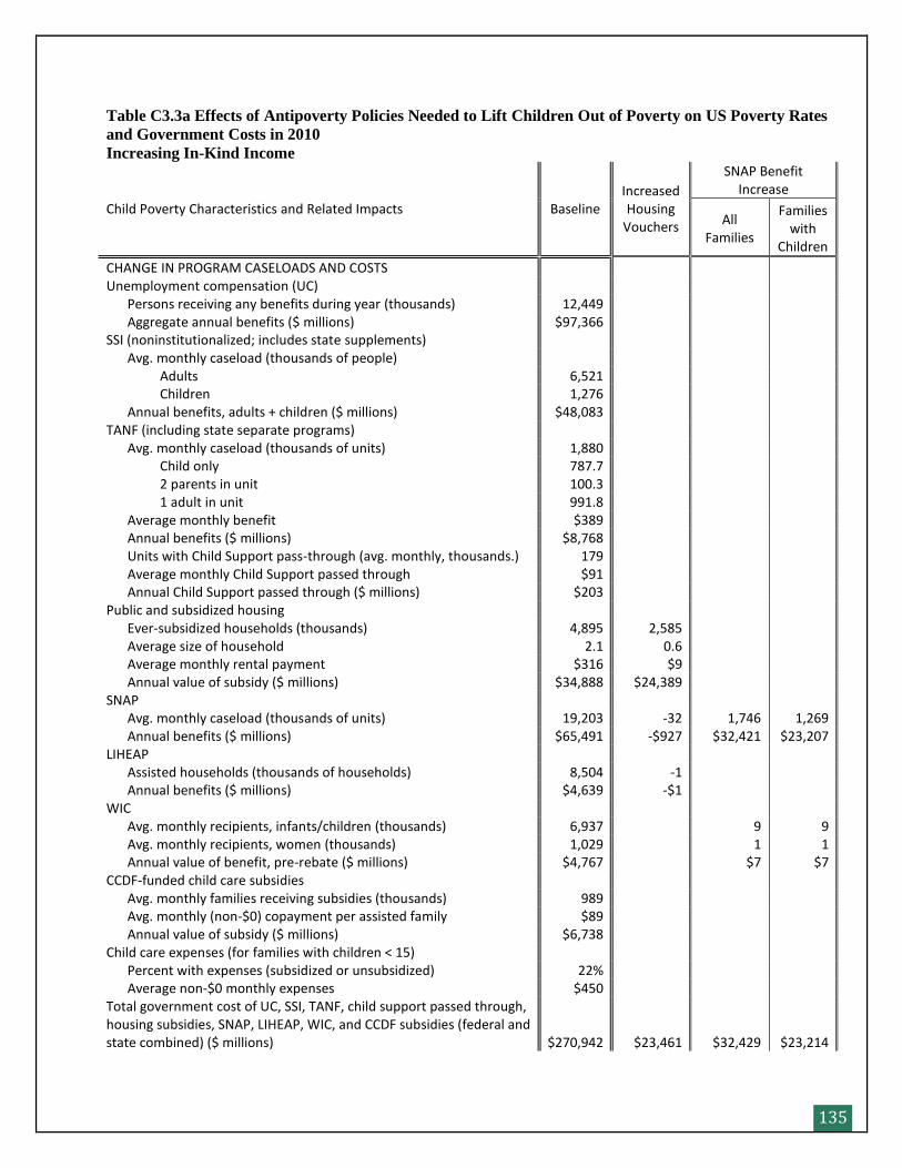
135
Table C3.3a Effects of Antipoverty Policies Needed to Lift Children Out of Poverty on US Poverty Rates
and Government Costs in 2010 Increasing In-Kind Income
Child Poverty Characteristics and Related Impacts Baseline Increased Housing
Vouchers
SNAP Benefit Increase
All Families
Families with
Children
CHANGE IN PROGRAM CASELOADS AND COSTS Unemployment compensation (UC) Persons receiving any benefits during year (thousands) 12,449 Aggregate annual benefits ($ millions) $97,366 SSI (noninstitutionalized; includes state supplements) Avg. monthly caseload (thousands of people) Adults 6,521 Children 1,276 Annual benefits, adults + children ($ millions) $48,083 TANF (including state separate programs) Avg. monthly caseload (thousands of units) 1,880 Child only 787.7 2 parents in unit 100.3 1 adult in unit 991.8 Average monthly benefit $389 Annual benefits ($ millions) $8,768 Units with Child Support pass-through (avg. monthly, thousands.) 179 Average monthly Child Support passed through $91 Annual Child Support passed through ($ millions) $203 Public and subsidized housing Ever-subsidized households (thousands) 4,895 2,585 Average size of household 2.1 0.6 Average monthly rental payment $316 $9 Annual value of subsidy ($ millions) $34,888 $24,389 SNAP Avg. monthly caseload (thousands of units) 19,203 -32 1,746 1,269 Annual benefits ($ millions) $65,491 -$927 $32,421 $23,207 LIHEAP Assisted households (thousands of households) 8,504 -1 Annual benefits ($ millions) $4,639 -$1 WIC Avg. monthly recipients, infants/children (thousands) 6,937 9 9 Avg. monthly recipients, women (thousands) 1,029 1 1 Annual value of benefit, pre-rebate ($ millions) $4,767 $7 $7 CCDF-funded child care subsidies Avg. monthly families receiving subsidies (thousands) 989 Avg. monthly (non-$0) copayment per assisted family $89 Annual value of subsidy ($ millions) $6,738 Child care expenses (for families with children < 15) Percent with expenses (subsidized or unsubsidized) 22% Average non-$0 monthly expenses $450 Total government cost of UC, SSI, TANF, child support passed through, housing subsidies, SNAP, LIHEAP, WIC, and CCDF subsidies (federal and state combined) ($ millions) $270,942 $23,461 $32,429 $23,214
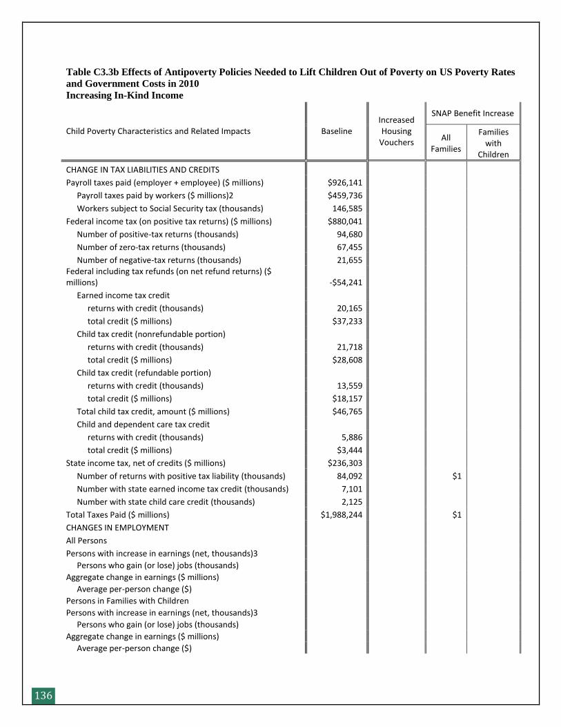
136
Table C3.3b Effects of Antipoverty Policies Needed to Lift Children Out of Poverty on US Poverty Rates
and Government Costs in 2010 Increasing In-Kind Income
Child Poverty Characteristics and Related Impacts Baseline Increased Housing
Vouchers
SNAP Benefit Increase
All Families
Families with
Children
CHANGE IN TAX LIABILITIES AND CREDITS
Payroll taxes paid (employer + employee) ($ millions) $926,141
Payroll taxes paid by workers ($ millions)2 $459,736
Workers subject to Social Security tax (thousands) 146,585
Federal income tax (on positive tax returns) ($ millions) $880,041
Number of positive-tax returns (thousands) 94,680
Number of zero-tax returns (thousands) 67,455
Number of negative-tax returns (thousands) 21,655 Federal including tax refunds (on net refund returns) ($ millions) -$54,241
Earned income tax credit
returns with credit (thousands) 20,165
total credit ($ millions) $37,233
Child tax credit (nonrefundable portion)
returns with credit (thousands) 21,718
total credit ($ millions) $28,608
Child tax credit (refundable portion)
returns with credit (thousands) 13,559
total credit ($ millions) $18,157
Total child tax credit, amount ($ millions) $46,765
Child and dependent care tax credit
returns with credit (thousands) 5,886
total credit ($ millions) $3,444
State income tax, net of credits ($ millions) $236,303
Number of returns with positive tax liability (thousands) 84,092 $1
Number with state earned income tax credit (thousands) 7,101
Number with state child care credit (thousands) 2,125
Total Taxes Paid ($ millions) $1,988,244 $1
CHANGES IN EMPLOYMENT
All Persons
Persons with increase in earnings (net, thousands)3
Persons who gain (or lose) jobs (thousands)
Aggregate change in earnings ($ millions)
Average per-person change ($)
Persons in Families with Children
Persons with increase in earnings (net, thousands)3
Persons who gain (or lose) jobs (thousands)
Aggregate change in earnings ($ millions)
Average per-person change ($)
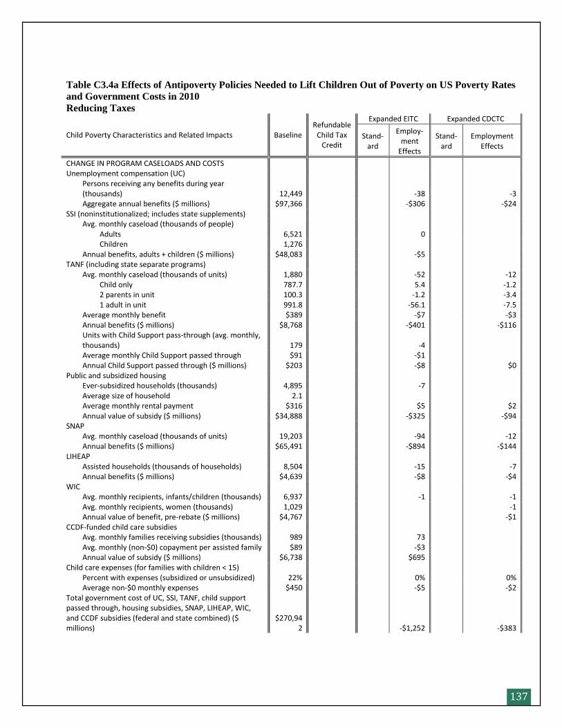
137
Table C3.4a Effects of Antipoverty Policies Needed to Lift Children Out of Poverty on US Poverty Rates
and Government Costs in 2010 Reducing Taxes
Child Poverty Characteristics and Related Impacts Baseline Refundable
Child Tax Credit
Expanded EITC Expanded CDCTC
Stand-ard
Employ-ment
Effects
Stand-ard
Employment Effects
CHANGE IN PROGRAM CASELOADS AND COSTS Unemployment compensation (UC)
Persons receiving any benefits during year (thousands) 12,449 -38 -3
Aggregate annual benefits ($ millions) $97,366 -$306 -$24 SSI (noninstitutionalized; includes state supplements) Avg. monthly caseload (thousands of people) Adults 6,521 0 Children 1,276 Annual benefits, adults + children ($ millions) $48,083 -$5 TANF (including state separate programs) Avg. monthly caseload (thousands of units) 1,880 -52 -12 Child only 787.7 5.4 -1.2 2 parents in unit 100.3 -1.2 -3.4 1 adult in unit 991.8 -56.1 -7.5 Average monthly benefit $389 -$7 -$3 Annual benefits ($ millions) $8,768 -$401 -$116
Units with Child Support pass-through (avg. monthly, thousands) 179 -4
Average monthly Child Support passed through $91 -$1 Annual Child Support passed through ($ millions) $203 -$8 $0 Public and subsidized housing Ever-subsidized households (thousands) 4,895 -7 Average size of household 2.1 Average monthly rental payment $316 $5 $2 Annual value of subsidy ($ millions) $34,888 -$325 -$94 SNAP Avg. monthly caseload (thousands of units) 19,203 -94 -12 Annual benefits ($ millions) $65,491 -$894 -$144 LIHEAP Assisted households (thousands of households) 8,504 -15 -7 Annual benefits ($ millions) $4,639 -$8 -$4 WIC Avg. monthly recipients, infants/children (thousands) 6,937 -1 -1 Avg. monthly recipients, women (thousands) 1,029 -1 Annual value of benefit, pre-rebate ($ millions) $4,767 -$1 CCDF-funded child care subsidies Avg. monthly families receiving subsidies (thousands) 989 73 Avg. monthly (non-$0) copayment per assisted family $89 -$3 Annual value of subsidy ($ millions) $6,738 $695 Child care expenses (for families with children < 15) Percent with expenses (subsidized or unsubsidized) 22% 0% 0% Average non-$0 monthly expenses $450 -$5 -$2 Total government cost of UC, SSI, TANF, child support passed through, housing subsidies, SNAP, LIHEAP, WIC, and CCDF subsidies (federal and state combined) ($ millions)
$270,942 -$1,252 -$383
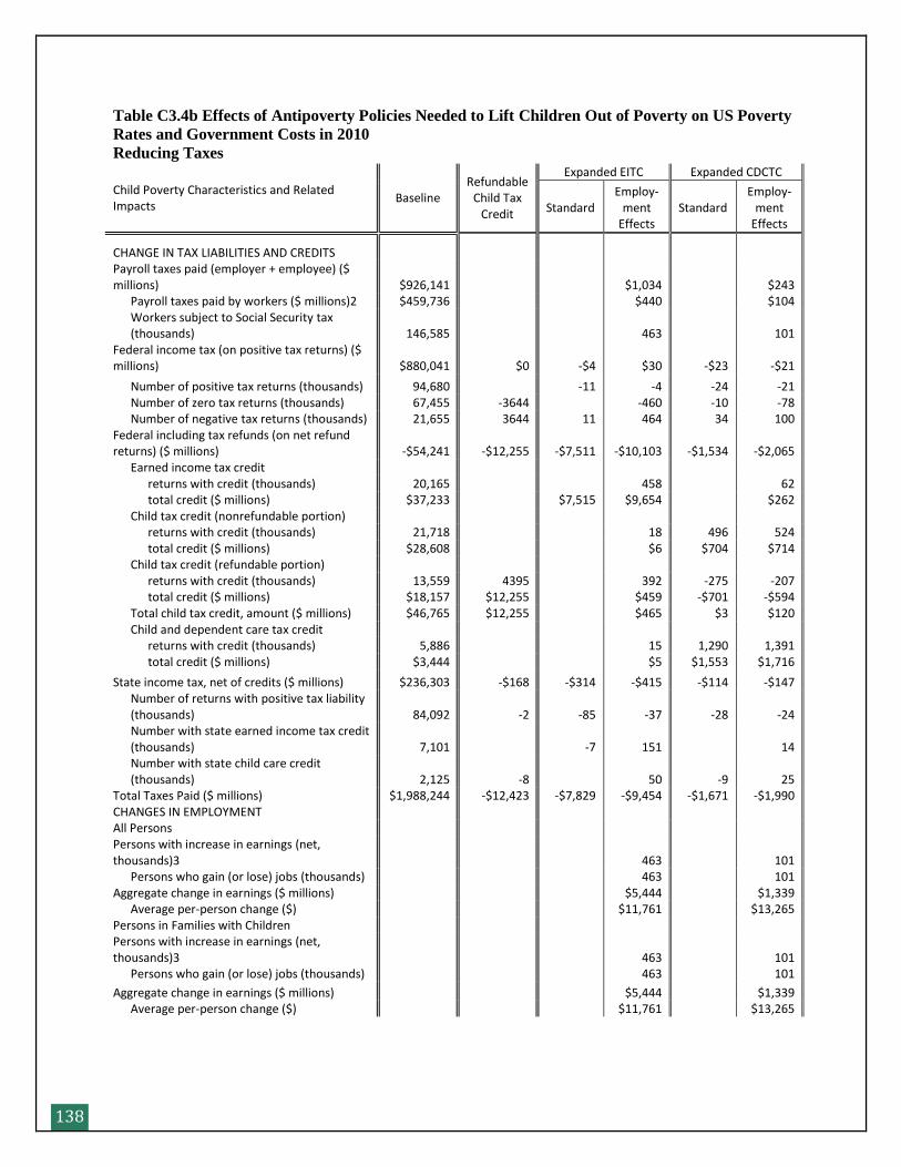
138
Table C3.4b Effects of Antipoverty Policies Needed to Lift Children Out of Poverty on US Poverty
Rates and Government Costs in 2010 Reducing Taxes
Child Poverty Characteristics and Related Impacts
Baseline Refundable
Child Tax Credit
Expanded EITC Expanded CDCTC
Standard Employ-
ment Effects
Standard Employ-
ment Effects
CHANGE IN TAX LIABILITIES AND CREDITS Payroll taxes paid (employer + employee) ($ millions) $926,141 $1,034 $243 Payroll taxes paid by workers ($ millions)2 $459,736 $440 $104
Workers subject to Social Security tax (thousands) 146,585 463 101
Federal income tax (on positive tax returns) ($ millions) $880,041 $0 -$4 $30 -$23 -$21
Number of positive tax returns (thousands) 94,680 -11 -4 -24 -21 Number of zero tax returns (thousands) 67,455 -3644 -460 -10 -78 Number of negative tax returns (thousands) 21,655 3644 11 464 34 100 Federal including tax refunds (on net refund returns) ($ millions) -$54,241 -$12,255 -$7,511 -$10,103 -$1,534 -$2,065 Earned income tax credit returns with credit (thousands) 20,165 458 62 total credit ($ millions) $37,233 $7,515 $9,654 $262 Child tax credit (nonrefundable portion) returns with credit (thousands) 21,718 18 496 524 total credit ($ millions) $28,608 $6 $704 $714 Child tax credit (refundable portion) returns with credit (thousands) 13,559 4395 392 -275 -207 total credit ($ millions) $18,157 $12,255 $459 -$701 -$594 Total child tax credit, amount ($ millions) $46,765 $12,255 $465 $3 $120 Child and dependent care tax credit returns with credit (thousands) 5,886 15 1,290 1,391 total credit ($ millions) $3,444 $5 $1,553 $1,716
State income tax, net of credits ($ millions) $236,303 -$168 -$314 -$415 -$114 -$147
Number of returns with positive tax liability (thousands) 84,092 -2 -85 -37 -28 -24
Number with state earned income tax credit (thousands) 7,101 -7 151 14
Number with state child care credit (thousands) 2,125 -8 50 -9 25
Total Taxes Paid ($ millions) $1,988,244 -$12,423 -$7,829 -$9,454 -$1,671 -$1,990 CHANGES IN EMPLOYMENT All Persons Persons with increase in earnings (net, thousands)3 463 101 Persons who gain (or lose) jobs (thousands) 463 101 Aggregate change in earnings ($ millions) $5,444 $1,339 Average per-person change ($) $11,761 $13,265 Persons in Families with Children Persons with increase in earnings (net, thousands)3 463 101 Persons who gain (or lose) jobs (thousands) 463 101
Aggregate change in earnings ($ millions) $5,444 $1,339 Average per-person change ($) $11,761 $13,265
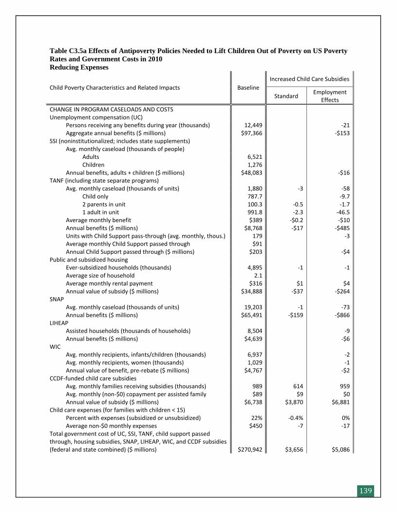
139
Table C3.5a Effects of Antipoverty Policies Needed to Lift Children Out of Poverty on US Poverty
Rates and Government Costs in 2010 Reducing Expenses
Child Poverty Characteristics and Related Impacts Baseline
Increased Child Care Subsidies
Standard Employment
Effects
CHANGE IN PROGRAM CASELOADS AND COSTS Unemployment compensation (UC) Persons receiving any benefits during year (thousands) 12,449 -21 Aggregate annual benefits ($ millions) $97,366 -$153 SSI (noninstitutionalized; includes state supplements) Avg. monthly caseload (thousands of people) Adults 6,521 Children 1,276 Annual benefits, adults + children ($ millions) $48,083 -$16 TANF (including state separate programs) Avg. monthly caseload (thousands of units) 1,880 -3 -58 Child only 787.7 -9.7 2 parents in unit 100.3 -0.5 -1.7 1 adult in unit 991.8 -2.3 -46.5 Average monthly benefit $389 -$0.2 -$10 Annual benefits ($ millions) $8,768 -$17 -$485 Units with Child Support pass-through (avg. monthly, thous.) 179 -3 Average monthly Child Support passed through $91 Annual Child Support passed through ($ millions) $203 -$4 Public and subsidized housing Ever-subsidized households (thousands) 4,895 -1 -1 Average size of household 2.1 Average monthly rental payment $316 $1 $4 Annual value of subsidy ($ millions) $34,888 -$37 -$264 SNAP Avg. monthly caseload (thousands of units) 19,203 -1 -73 Annual benefits ($ millions) $65,491 -$159 -$866 LIHEAP Assisted households (thousands of households) 8,504 -9 Annual benefits ($ millions) $4,639 -$6 WIC Avg. monthly recipients, infants/children (thousands) 6,937 -2 Avg. monthly recipients, women (thousands) 1,029 -1 Annual value of benefit, pre-rebate ($ millions) $4,767 -$2 CCDF-funded child care subsidies Avg. monthly families receiving subsidies (thousands) 989 614 959 Avg. monthly (non-$0) copayment per assisted family $89 $9 $0 Annual value of subsidy ($ millions) $6,738 $3,870 $6,881 Child care expenses (for families with children < 15) Percent with expenses (subsidized or unsubsidized) 22% -0.4% 0% Average non-$0 monthly expenses $450 -7 -17 Total government cost of UC, SSI, TANF, child support passed through, housing subsidies, SNAP, LIHEAP, WIC, and CCDF subsidies (federal and state combined) ($ millions) $270,942 $3,656 $5,086
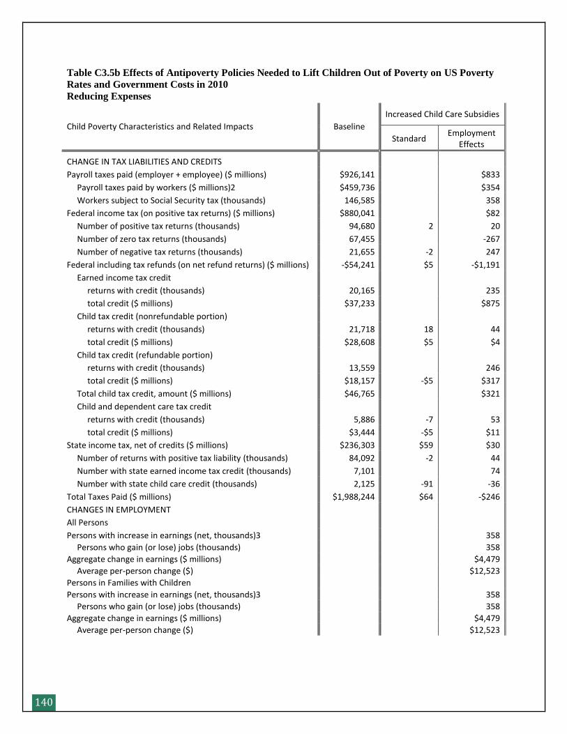
140
Table C3.5b Effects of Antipoverty Policies Needed to Lift Children Out of Poverty on US Poverty
Rates and Government Costs in 2010 Reducing Expenses
Child Poverty Characteristics and Related Impacts Baseline
Increased Child Care Subsidies
Standard Employment
Effects
CHANGE IN TAX LIABILITIES AND CREDITS
Payroll taxes paid (employer + employee) ($ millions) $926,141 $833
Payroll taxes paid by workers ($ millions)2 $459,736 $354
Workers subject to Social Security tax (thousands) 146,585 358
Federal income tax (on positive tax returns) ($ millions) $880,041 $82
Number of positive tax returns (thousands) 94,680 2 20
Number of zero tax returns (thousands) 67,455 -267
Number of negative tax returns (thousands) 21,655 -2 247
Federal including tax refunds (on net refund returns) ($ millions) -$54,241 $5 -$1,191
Earned income tax credit
returns with credit (thousands) 20,165 235
total credit ($ millions) $37,233 $875
Child tax credit (nonrefundable portion)
returns with credit (thousands) 21,718 18 44
total credit ($ millions) $28,608 $5 $4
Child tax credit (refundable portion)
returns with credit (thousands) 13,559 246
total credit ($ millions) $18,157 -$5 $317
Total child tax credit, amount ($ millions) $46,765 $321
Child and dependent care tax credit
returns with credit (thousands) 5,886 -7 53
total credit ($ millions) $3,444 -$5 $11
State income tax, net of credits ($ millions) $236,303 $59 $30
Number of returns with positive tax liability (thousands) 84,092 -2 44
Number with state earned income tax credit (thousands) 7,101 74
Number with state child care credit (thousands) 2,125 -91 -36
Total Taxes Paid ($ millions) $1,988,244 $64 -$246
CHANGES IN EMPLOYMENT
All Persons
Persons with increase in earnings (net, thousands)3 358
Persons who gain (or lose) jobs (thousands) 358
Aggregate change in earnings ($ millions) $4,479
Average per-person change ($) $12,523
Persons in Families with Children
Persons with increase in earnings (net, thousands)3 358
Persons who gain (or lose) jobs (thousands) 358
Aggregate change in earnings ($ millions) $4,479
Average per-person change ($) $12,523
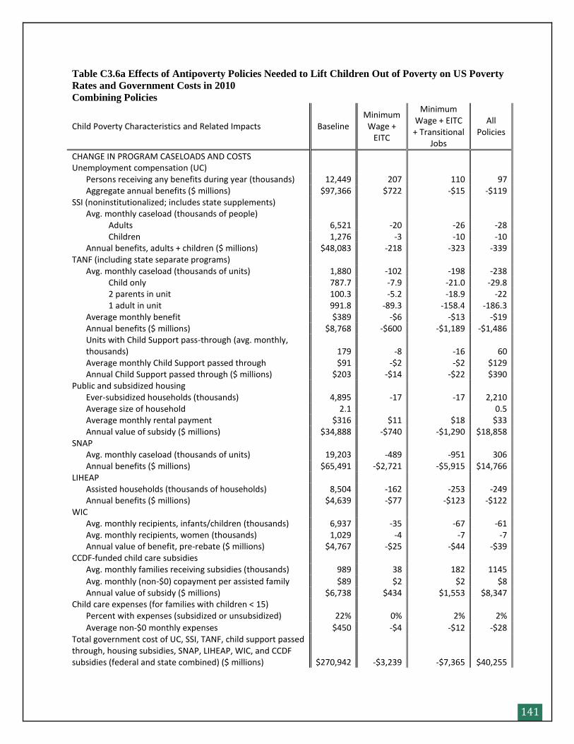
141
Table C3.6a Effects of Antipoverty Policies Needed to Lift Children Out of Poverty on US Poverty
Rates and Government Costs in 2010 Combining Policies
Child Poverty Characteristics and Related Impacts Baseline Minimum
Wage + EITC
Minimum Wage + EITC
+ Transitional Jobs
All Policies
CHANGE IN PROGRAM CASELOADS AND COSTS Unemployment compensation (UC) Persons receiving any benefits during year (thousands) 12,449 207 110 97 Aggregate annual benefits ($ millions) $97,366 $722 -$15 -$119 SSI (noninstitutionalized; includes state supplements) Avg. monthly caseload (thousands of people) Adults 6,521 -20 -26 -28 Children 1,276 -3 -10 -10 Annual benefits, adults + children ($ millions) $48,083 -218 -323 -339 TANF (including state separate programs) Avg. monthly caseload (thousands of units) 1,880 -102 -198 -238 Child only 787.7 -7.9 -21.0 -29.8 2 parents in unit 100.3 -5.2 -18.9 -22 1 adult in unit 991.8 -89.3 -158.4 -186.3 Average monthly benefit $389 -$6 -$13 -$19 Annual benefits ($ millions) $8,768 -$600 -$1,189 -$1,486
Units with Child Support pass-through (avg. monthly, thousands) 179 -8 -16 60
Average monthly Child Support passed through $91 -$2 -$2 $129 Annual Child Support passed through ($ millions) $203 -$14 -$22 $390 Public and subsidized housing Ever-subsidized households (thousands) 4,895 -17 -17 2,210 Average size of household 2.1 0.5 Average monthly rental payment $316 $11 $18 $33 Annual value of subsidy ($ millions) $34,888 -$740 -$1,290 $18,858 SNAP Avg. monthly caseload (thousands of units) 19,203 -489 -951 306 Annual benefits ($ millions) $65,491 -$2,721 -$5,915 $14,766 LIHEAP Assisted households (thousands of households) 8,504 -162 -253 -249 Annual benefits ($ millions) $4,639 -$77 -$123 -$122 WIC Avg. monthly recipients, infants/children (thousands) 6,937 -35 -67 -61 Avg. monthly recipients, women (thousands) 1,029 -4 -7 -7 Annual value of benefit, pre-rebate ($ millions) $4,767 -$25 -$44 -$39 CCDF-funded child care subsidies Avg. monthly families receiving subsidies (thousands) 989 38 182 1145
Avg. monthly (non-$0) copayment per assisted family $89 $2 $2 $8 Annual value of subsidy ($ millions) $6,738 $434 $1,553 $8,347 Child care expenses (for families with children < 15) Percent with expenses (subsidized or unsubsidized) 22% 0% 2% 2%
Average non-$0 monthly expenses $450 -$4 -$12 -$28 Total government cost of UC, SSI, TANF, child support passed through, housing subsidies, SNAP, LIHEAP, WIC, and CCDF subsidies (federal and state combined) ($ millions) $270,942 -$3,239 -$7,365 $40,255
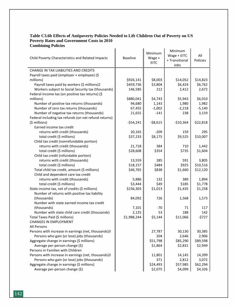
142
Table C3.6b Effects of Antipoverty Policies Needed to Lift Children Out of Poverty on US
Poverty Rates and Government Costs in 2010 Combining Policies
Child Poverty Characteristics and Related Impacts Baseline Minimum
Wage + EITC
Minimum Wage + EITC
+ Transitional Jobs
All Policies
CHANGE IN TAX LIABILITIES AND CREDITS Payroll taxes paid (employer + employee) ($ millions) $926,141 $8,003 $14,052 $14,823 Payroll taxes paid by workers ($ millions)2 $459,736 $3,804 $6,424 $6,762 Workers subject to Social Security tax (thousands) 146,585 212 2,412 2,672 Federal income tax (on positive tax returns) ($ millions) $880,041 $4,743 $5,943 $6,010 Number of positive tax returns (thousands) 94,680 1,143 1,980 1,982 Number of zero tax returns (thousands) 67,455 -1,002 -2,218 -5,140 Number of negative tax returns (thousands) 21,655 -141 238 3,159 Federal including tax refunds (on net refund returns) ($ millions) -$54,241 -$8,615 -$10,364 -$22,818 Earned income tax credit returns with credit (thousands) 20,165 -209 159 295 total credit ($ millions) $37,233 $8,175 $9,525 $10,007 Child tax credit (nonrefundable portion) returns with credit (thousands) 21,718 384 710 1,442 total credit ($ millions) $28,608 $354 $735 $1,604 Child tax credit (refundable portion) returns with credit (thousands) 13,559 285 591 3,805 total credit ($ millions) $18,157 $484 $925 $10,516 Total child tax credit, amount ($ millions) $46,765 $838 $1,660 $12,120 Child and dependent care tax credit returns with credit (thousands) 5,886 132 389 1,894 total credit ($ millions) $3,444 $49 $185 $1,778 State income tax, net of credits ($ millions) $236,303 $1,013 $1,435 $1,258
Number of returns with positive tax liability (thousands) 84,092 726 1,568 1,573
Number with state earned income tax credit (thousands) 7,101 -70 71 117
Number with state child care credit (thousands) 2,125 53 188 142 Total Taxes Paid ($ millions) $1,988,244 $5,144 $11,066 -$727 CHANGES IN EMPLOYMENT All Persons Persons with increase in earnings (net, thousands)3 27,787 30,130 30,385 Persons who gain (or lose) jobs (thousands) 204 2,646 2,906 Aggregate change in earnings ($ millions) $51,798 $85,290 $89,598 Average per-person change ($) $1,864 $2,831 $2,949 Persons in Families with Children Persons with increase in earnings (net, thousands)3 11,801 14,145 14,399 Persons who gain (or lose) jobs (thousands) 371 2,812 3,072 Aggregate change in earnings ($ millions) $24,493 $57,985 $62,294 Average per-person change ($) $2,075 $4,099 $4,326
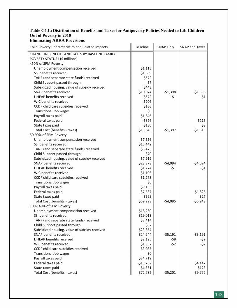
143
Table C4.1a Distribution of Benefits and Taxes for Antipoverty Policies Needed to Lift Children
Out of Poverty in 2010 Eliminating ARRA Provisions
Child Poverty Characteristics and Related Impacts Baseline SNAP Only SNAP and Taxes
CHANGE IN BENEFITS AND TAXES BY BASELINE FAMILY POVERTY STATUS1 ($ millions) <50% of SPM Poverty Unemployment compensation received $1,115 SSI benefits received $1,659 TANF (and separate state funds) received $572 Child Support passed through $7 Subsidized housing, value of subsidy received $443 SNAP benefits received $10,074 -$1,398 -$1,398 LIHEAP benefits received $572 $1 $1 WIC benefits received $206 CCDF child care subsidies received $166 Transitional Job wages $0 Payroll taxes paid $1,846 Federal taxes paid -$826 $213 State taxes paid $150 $3 Total Cost (benefits - taxes) $13,643 -$1,397 -$1,613 50-99% of SPM Poverty Unemployment compensation received $7,556 SSI benefits received $15,442 TANF (and separate state funds) received $3,475 Child Support passed through $70 Subsidized housing, value of subsidy received $7,919 SNAP benefits received $23,378 -$4,094 -$4,094 LIHEAP benefits received $1,274 -$1 -$1 WIC benefits received $1,105 CCDF child care subsidies received $1,273 Transitional Job wages $0 Payroll taxes paid $9,135 Federal taxes paid -$7,637 $1,826 State taxes paid $695 $27 Total Cost (benefits - taxes) $59,298 -$4,095 -$5,948 100-149% of SPM Poverty Unemployment compensation received $18,260 SSI benefits received $19,013 TANF (and separate state funds) received $3,414 Child Support passed through $87 Subsidized housing, value of subsidy received $23,864 SNAP benefits received $24,244 -$5,191 -$5,191 LIHEAP benefits received $2,125 -$9 -$9 WIC benefits received $1,957 -$2 -$2 CCDF child care subsidies received $3,085 Transitional Job wages $0 Payroll taxes paid $34,719 Federal taxes paid -$15,762 $4,447 State taxes paid $4,361 $123 Total Cost (benefits - taxes) $72,732 -$5,201 -$9,772
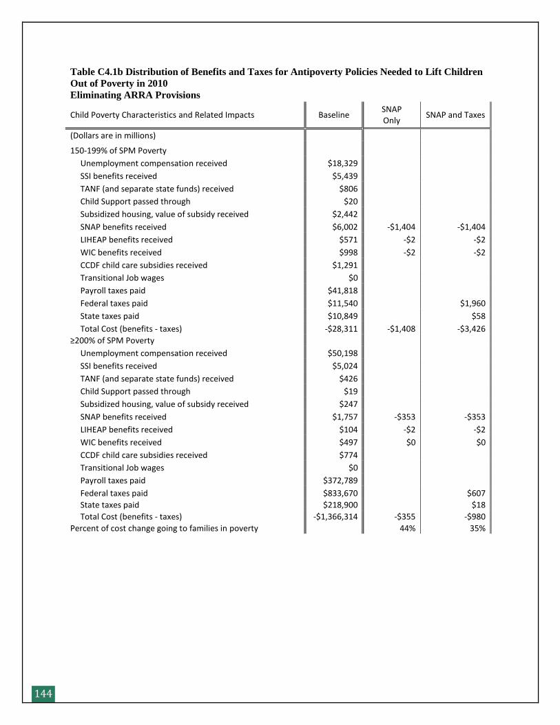
144
Table C4.1b Distribution of Benefits and Taxes for Antipoverty Policies Needed to Lift Children
Out of Poverty in 2010 Eliminating ARRA Provisions
Child Poverty Characteristics and Related Impacts Baseline SNAP Only
SNAP and Taxes
(Dollars are in millions)
150-199% of SPM Poverty
Unemployment compensation received $18,329
SSI benefits received $5,439
TANF (and separate state funds) received $806
Child Support passed through $20
Subsidized housing, value of subsidy received $2,442
SNAP benefits received $6,002 -$1,404 -$1,404
LIHEAP benefits received $571 -$2 -$2
WIC benefits received $998 -$2 -$2
CCDF child care subsidies received $1,291
Transitional Job wages $0
Payroll taxes paid $41,818
Federal taxes paid $11,540 $1,960
State taxes paid $10,849 $58
Total Cost (benefits - taxes) -$28,311 -$1,408 -$3,426
≥200% of SPM Poverty
Unemployment compensation received $50,198
SSI benefits received $5,024
TANF (and separate state funds) received $426
Child Support passed through $19
Subsidized housing, value of subsidy received $247
SNAP benefits received $1,757 -$353 -$353
LIHEAP benefits received $104 -$2 -$2
WIC benefits received $497 $0 $0
CCDF child care subsidies received $774
Transitional Job wages $0
Payroll taxes paid $372,789
Federal taxes paid $833,670 $607
State taxes paid $218,900 $18
Total Cost (benefits - taxes) -$1,366,314 -$355 -$980
Percent of cost change going to families in poverty 44% 35%
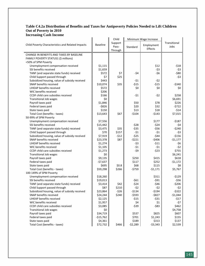
145
Table C4.2a Distribution of Benefits and Taxes for Antipoverty Policies Needed to Lift Children
Out of Poverty in 2010 Increasing Cash Income
Child Poverty Characteristics and Related Impacts Baseline
Child Support
Pass-Through
Minimum Wage Increase Transitional
Jobs Standard Employment
Effects
CHANGE IN BENEFITS AND TAXES BY BASELINE FAMILY POVERTY STATUS1 ($ millions) <50% of SPM Poverty Unemployment compensation received $1,115 $12 -$18 SSI benefits received $1,659 -$3 -$3 TANF (and separate state funds) received $572 $7 -$4 -$6 -$80 Child Support passed through $7 $25 -$3 Subsidized housing, value of subsidy received $443 -$1 -$2 SNAP benefits received $10,074 $35 -$15 -$15 -$340 LIHEAP benefits received $572 $0 $0 $0 WIC benefits received $206 CCDF child care subsidies received $166 -$1 -$2 $258 Transitional Job wages $0 $6,691 Payroll taxes paid $1,846 $50 $78 $226 Federal taxes paid -$826 $20 $32 -$722 State taxes paid $150 $13 $18 -$14 Total Cost (benefits - taxes) $13,643 $67 -$104 -$143 $7,015 50-99% of SPM Poverty Unemployment compensation received $7,556 $177 -$187 SSI benefits received $15,442 -$28 -$24 -$4 TANF (and separate state funds) received $3,475 $35 -$35 -$56 -$240 Child Support passed through $70 $157 -$1 -$1 -$3 Subsidized housing, value of subsidy received $7,919 -$12 -$25 -$44 -$156 SNAP benefits received $23,378 $87 -$221 -$406 -$1,177 LIHEAP benefits received $1,274 -$3 -$11 -$6 WIC benefits received $1,105 -$1 -$1 -$2 CCDF child care subsidies received $1,273 -$9 -$23 $755 Transitional Job wages $0 $6,241 Payroll taxes paid $9,135 $250 $415 $618 Federal taxes paid -$7,637 $117 $252 -$1,172 State taxes paid $695 $0.8 $68 $115 $8 Total Cost (benefits - taxes) $59,298 $266 -$759 -$1,171 $5,767 100-149% of SPM Poverty Unemployment compensation received $18,260 $311 -$129 SSI benefits received $19,013 -$61 -$91 -$56 TANF (and separate state funds) received $3,414 $42 -$24 -$46 -$206 Child Support passed through $87 $210 -$2 -$2 -$2 Subsidized housing, value of subsidy received $23,864 -$26 -$134 -$194 -$322 SNAP benefits received $24,244 $240 -$593 -$827 -$1,044 LIHEAP benefits received $2,125 -$15 -$31 -$17 WIC benefits received $1,957 $4 $1 -$7 CCDF child care subsidies received $3,085 -$39 -$83 $462 Transitional Job wages $0 $4,758 Payroll taxes paid $34,719 $537 $825 $607 Federal taxes paid -$15,762 $701 $1,243 $155 State taxes paid $4,361 $189 $313 $137 Total Cost (benefits - taxes) $72,732 $466 -$2,289 -$3,343 $2,539
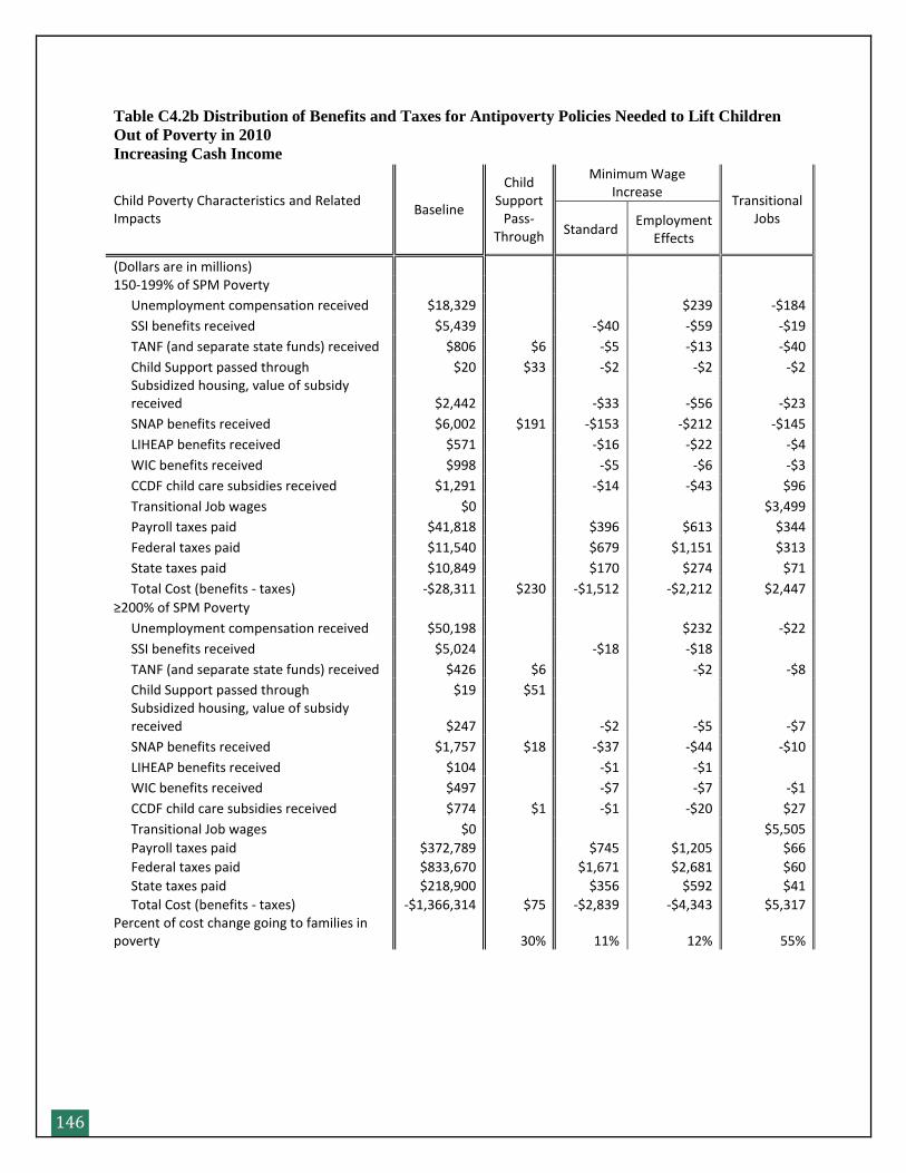
146
Table C4.2b Distribution of Benefits and Taxes for Antipoverty Policies Needed to Lift Children
Out of Poverty in 2010 Increasing Cash Income
Child Poverty Characteristics and Related Impacts
Baseline
Child Support
Pass-Through
Minimum Wage Increase
Transitional Jobs
Standard Employment
Effects
(Dollars are in millions) 150-199% of SPM Poverty
Unemployment compensation received $18,329 $239 -$184
SSI benefits received $5,439 -$40 -$59 -$19
TANF (and separate state funds) received $806 $6 -$5 -$13 -$40
Child Support passed through $20 $33 -$2 -$2 -$2
Subsidized housing, value of subsidy received $2,442 -$33 -$56 -$23
SNAP benefits received $6,002 $191 -$153 -$212 -$145
LIHEAP benefits received $571 -$16 -$22 -$4
WIC benefits received $998 -$5 -$6 -$3
CCDF child care subsidies received $1,291 -$14 -$43 $96
Transitional Job wages $0 $3,499
Payroll taxes paid $41,818 $396 $613 $344
Federal taxes paid $11,540 $679 $1,151 $313
State taxes paid $10,849 $170 $274 $71
Total Cost (benefits - taxes) -$28,311 $230 -$1,512 -$2,212 $2,447
≥200% of SPM Poverty
Unemployment compensation received $50,198 $232 -$22
SSI benefits received $5,024 -$18 -$18
TANF (and separate state funds) received $426 $6 -$2 -$8
Child Support passed through $19 $51
Subsidized housing, value of subsidy received $247 -$2 -$5 -$7
SNAP benefits received $1,757 $18 -$37 -$44 -$10
LIHEAP benefits received $104 -$1 -$1
WIC benefits received $497 -$7 -$7 -$1
CCDF child care subsidies received $774 $1 -$1 -$20 $27
Transitional Job wages $0 $5,505
Payroll taxes paid $372,789 $745 $1,205 $66
Federal taxes paid $833,670 $1,671 $2,681 $60
State taxes paid $218,900 $356 $592 $41
Total Cost (benefits - taxes) -$1,366,314 $75 -$2,839 -$4,343 $5,317 Percent of cost change going to families in poverty 30% 11% 12% 55%
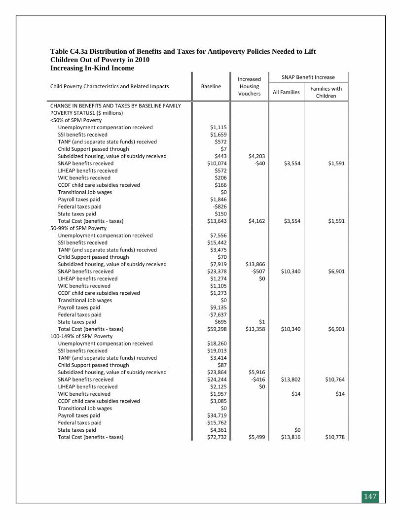
147
Table C4.3a Distribution of Benefits and Taxes for Antipoverty Policies Needed to Lift
Children Out of Poverty in 2010 Increasing In-Kind Income
Child Poverty Characteristics and Related Impacts Baseline Increased Housing
Vouchers
SNAP Benefit Increase
All Families Families with
Children
CHANGE IN BENEFITS AND TAXES BY BASELINE FAMILY POVERTY STATUS1 ($ millions) <50% of SPM Poverty Unemployment compensation received $1,115 SSI benefits received $1,659 TANF (and separate state funds) received $572 Child Support passed through $7 Subsidized housing, value of subsidy received $443 $4,203 SNAP benefits received $10,074 -$40 $3,554 $1,591 LIHEAP benefits received $572 WIC benefits received $206 CCDF child care subsidies received $166 Transitional Job wages $0 Payroll taxes paid $1,846 Federal taxes paid -$826 State taxes paid $150 Total Cost (benefits - taxes) $13,643 $4,162 $3,554 $1,591 50-99% of SPM Poverty Unemployment compensation received $7,556 SSI benefits received $15,442 TANF (and separate state funds) received $3,475 Child Support passed through $70 Subsidized housing, value of subsidy received $7,919 $13,866 SNAP benefits received $23,378 -$507 $10,340 $6,901 LIHEAP benefits received $1,274 $0 WIC benefits received $1,105 CCDF child care subsidies received $1,273 Transitional Job wages $0 Payroll taxes paid $9,135 Federal taxes paid -$7,637 State taxes paid $695 $1 Total Cost (benefits - taxes) $59,298 $13,358 $10,340 $6,901 100-149% of SPM Poverty Unemployment compensation received $18,260 SSI benefits received $19,013 TANF (and separate state funds) received $3,414 Child Support passed through $87 Subsidized housing, value of subsidy received $23,864 $5,916 SNAP benefits received $24,244 -$416 $13,802 $10,764 LIHEAP benefits received $2,125 $0 WIC benefits received $1,957 $14 $14 CCDF child care subsidies received $3,085 Transitional Job wages $0 Payroll taxes paid $34,719 Federal taxes paid -$15,762 State taxes paid $4,361 $0 Total Cost (benefits - taxes) $72,732 $5,499 $13,816 $10,778
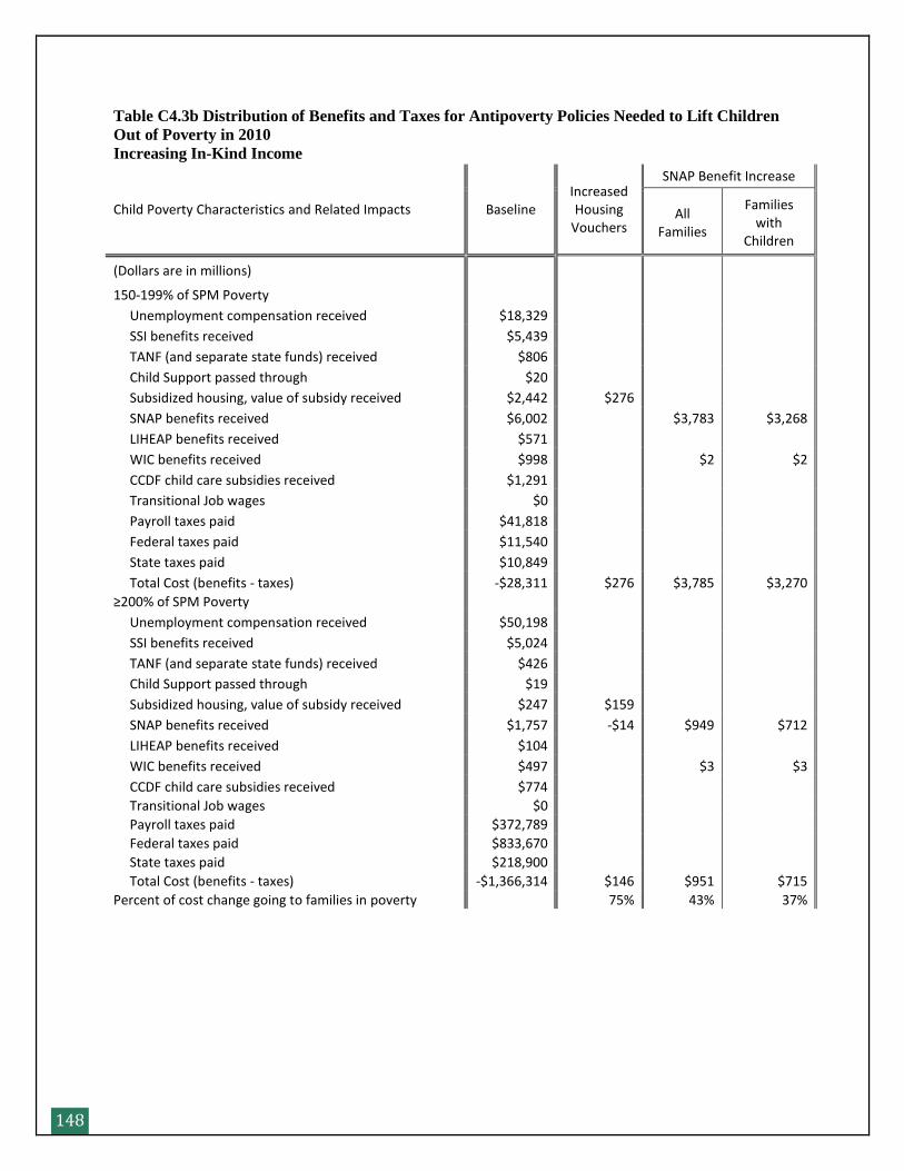
148
Table C4.3b Distribution of Benefits and Taxes for Antipoverty Policies Needed to Lift Children
Out of Poverty in 2010 Increasing In-Kind Income
Child Poverty Characteristics and Related Impacts Baseline Increased Housing
Vouchers
SNAP Benefit Increase
All Families
Families with
Children
(Dollars are in millions)
150-199% of SPM Poverty
Unemployment compensation received $18,329
SSI benefits received $5,439
TANF (and separate state funds) received $806
Child Support passed through $20
Subsidized housing, value of subsidy received $2,442 $276
SNAP benefits received $6,002 $3,783 $3,268
LIHEAP benefits received $571
WIC benefits received $998 $2 $2
CCDF child care subsidies received $1,291
Transitional Job wages $0
Payroll taxes paid $41,818
Federal taxes paid $11,540
State taxes paid $10,849
Total Cost (benefits - taxes) -$28,311 $276 $3,785 $3,270
≥200% of SPM Poverty
Unemployment compensation received $50,198
SSI benefits received $5,024
TANF (and separate state funds) received $426
Child Support passed through $19
Subsidized housing, value of subsidy received $247 $159
SNAP benefits received $1,757 -$14 $949 $712
LIHEAP benefits received $104
WIC benefits received $497 $3 $3
CCDF child care subsidies received $774
Transitional Job wages $0
Payroll taxes paid $372,789
Federal taxes paid $833,670
State taxes paid $218,900
Total Cost (benefits - taxes) -$1,366,314 $146 $951 $715
Percent of cost change going to families in poverty 75% 43% 37%
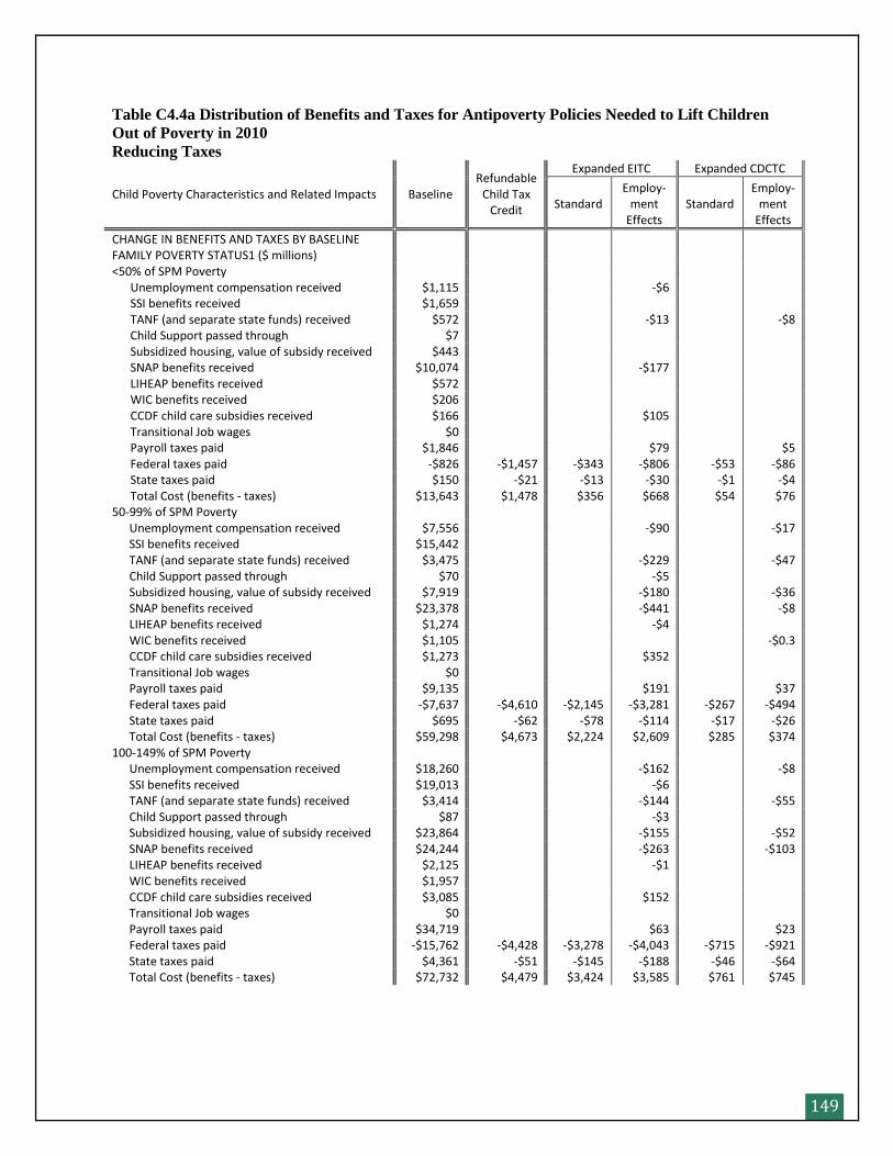
149
Table C4.4a Distribution of Benefits and Taxes for Antipoverty Policies Needed to Lift Children
Out of Poverty in 2010 Reducing Taxes
Child Poverty Characteristics and Related Impacts Baseline Refundable
Child Tax Credit
Expanded EITC Expanded CDCTC
Standard Employ-
ment Effects
Standard Employ-
ment Effects
CHANGE IN BENEFITS AND TAXES BY BASELINE FAMILY POVERTY STATUS1 ($ millions) <50% of SPM Poverty Unemployment compensation received $1,115 -$6 SSI benefits received $1,659 TANF (and separate state funds) received $572 -$13 -$8 Child Support passed through $7 Subsidized housing, value of subsidy received $443 SNAP benefits received $10,074 -$177 LIHEAP benefits received $572 WIC benefits received $206 CCDF child care subsidies received $166 $105 Transitional Job wages $0 Payroll taxes paid $1,846 $79 $5 Federal taxes paid -$826 -$1,457 -$343 -$806 -$53 -$86 State taxes paid $150 -$21 -$13 -$30 -$1 -$4 Total Cost (benefits - taxes) $13,643 $1,478 $356 $668 $54 $76 50-99% of SPM Poverty Unemployment compensation received $7,556 -$90 -$17 SSI benefits received $15,442 TANF (and separate state funds) received $3,475 -$229 -$47 Child Support passed through $70 -$5 Subsidized housing, value of subsidy received $7,919 -$180 -$36 SNAP benefits received $23,378 -$441 -$8 LIHEAP benefits received $1,274 -$4 WIC benefits received $1,105 -$0.3 CCDF child care subsidies received $1,273 $352 Transitional Job wages $0 Payroll taxes paid $9,135 $191 $37 Federal taxes paid -$7,637 -$4,610 -$2,145 -$3,281 -$267 -$494 State taxes paid $695 -$62 -$78 -$114 -$17 -$26 Total Cost (benefits - taxes) $59,298 $4,673 $2,224 $2,609 $285 $374 100-149% of SPM Poverty Unemployment compensation received $18,260 -$162 -$8 SSI benefits received $19,013 -$6 TANF (and separate state funds) received $3,414 -$144 -$55 Child Support passed through $87 -$3 Subsidized housing, value of subsidy received $23,864 -$155 -$52 SNAP benefits received $24,244 -$263 -$103 LIHEAP benefits received $2,125 -$1 WIC benefits received $1,957 CCDF child care subsidies received $3,085 $152 Transitional Job wages $0 Payroll taxes paid $34,719 $63 $23 Federal taxes paid -$15,762 -$4,428 -$3,278 -$4,043 -$715 -$921 State taxes paid $4,361 -$51 -$145 -$188 -$46 -$64 Total Cost (benefits - taxes) $72,732 $4,479 $3,424 $3,585 $761 $745
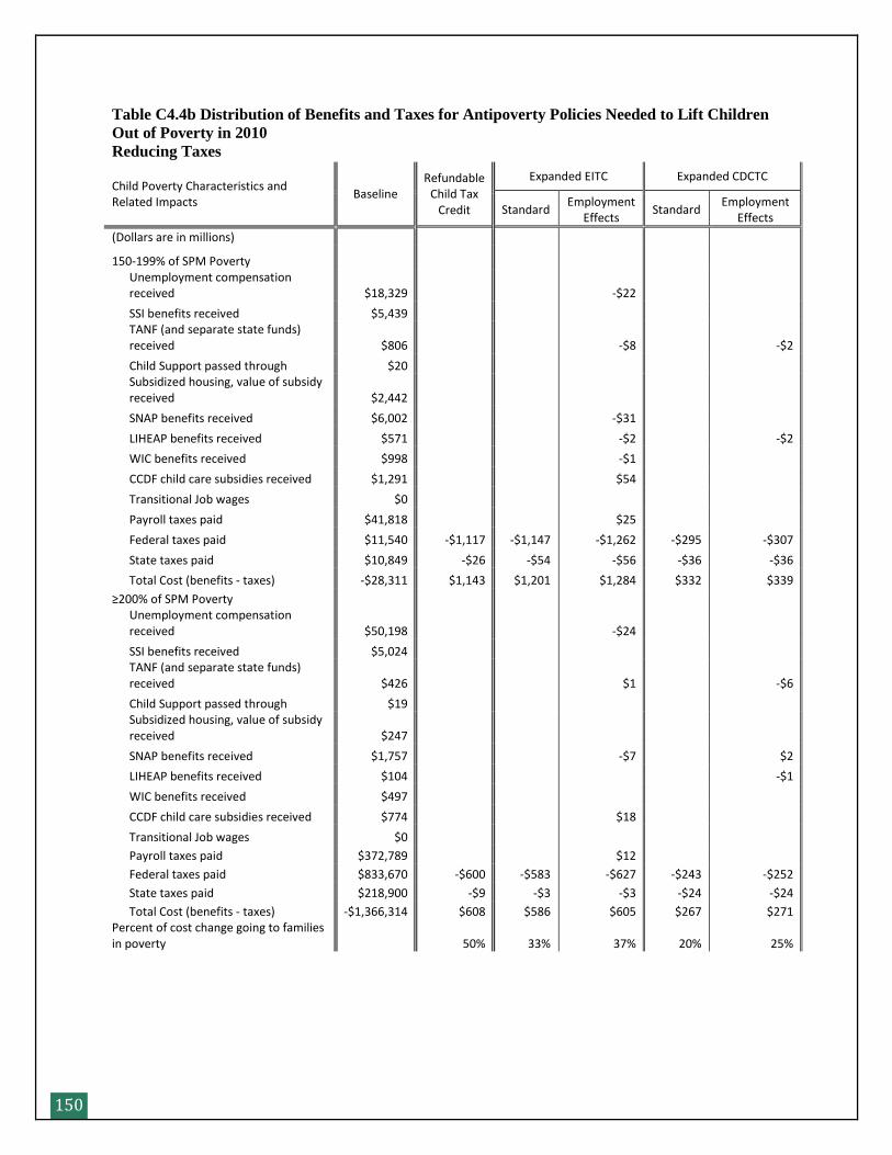
150
Table C4.4b Distribution of Benefits and Taxes for Antipoverty Policies Needed to Lift Children
Out of Poverty in 2010 Reducing Taxes
Child Poverty Characteristics and Related Impacts
Baseline Refundable
Child Tax Credit
Expanded EITC Expanded CDCTC
Standard Employment
Effects Standard
Employment Effects
(Dollars are in millions)
150-199% of SPM Poverty
Unemployment compensation received $18,329 -$22
SSI benefits received $5,439
TANF (and separate state funds) received $806 -$8 -$2
Child Support passed through $20
Subsidized housing, value of subsidy received $2,442
SNAP benefits received $6,002 -$31
LIHEAP benefits received $571 -$2 -$2
WIC benefits received $998 -$1
CCDF child care subsidies received $1,291 $54
Transitional Job wages $0
Payroll taxes paid $41,818 $25
Federal taxes paid $11,540 -$1,117 -$1,147 -$1,262 -$295 -$307
State taxes paid $10,849 -$26 -$54 -$56 -$36 -$36
Total Cost (benefits - taxes) -$28,311 $1,143 $1,201 $1,284 $332 $339
≥200% of SPM Poverty
Unemployment compensation received $50,198 -$24
SSI benefits received $5,024
TANF (and separate state funds) received $426 $1 -$6
Child Support passed through $19
Subsidized housing, value of subsidy received $247
SNAP benefits received $1,757 -$7 $2
LIHEAP benefits received $104 -$1
WIC benefits received $497
CCDF child care subsidies received $774 $18
Transitional Job wages $0
Payroll taxes paid $372,789 $12
Federal taxes paid $833,670 -$600 -$583 -$627 -$243 -$252
State taxes paid $218,900 -$9 -$3 -$3 -$24 -$24
Total Cost (benefits - taxes) -$1,366,314 $608 $586 $605 $267 $271 Percent of cost change going to families in poverty 50% 33% 37% 20% 25%
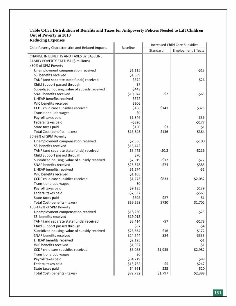
151
Table C4.5a Distribution of Benefits and Taxes for Antipoverty Policies Needed to Lift Children
Out of Poverty in 2010 Reducing Expenses
Child Poverty Characteristics and Related Impacts Baseline Increased Child Care Subsidies
Standard Employment Effects
CHANGE IN BENEFITS AND TAXES BY BASELINE FAMILY POVERTY STATUS1 ($ millions) <50% of SPM Poverty Unemployment compensation received $1,115 -$13 SSI benefits received $1,659 TANF (and separate state funds) received $572 -$26 Child Support passed through $7 Subsidized housing, value of subsidy received $443 SNAP benefits received $10,074 -$2 -$63 LIHEAP benefits received $572 WIC benefits received $206 CCDF child care subsidies received $166 $141 $325 Transitional Job wages $0 Payroll taxes paid $1,846 $36 Federal taxes paid -$826 -$177 State taxes paid $150 $3 $1 Total Cost (benefits - taxes) $13,643 $136 $364 50-99% of SPM Poverty Unemployment compensation received $7,556 -$100 SSI benefits received $15,442 TANF (and separate state funds) received $3,475 -$0.2 -$216 Child Support passed through $70 Subsidized housing, value of subsidy received $7,919 -$12 -$72 SNAP benefits received $23,378 -$74 -$385 LIHEAP benefits received $1,274 -$1 WIC benefits received $1,105 CCDF child care subsidies received $1,273 $833 $2,052 Transitional Job wages $0 Payroll taxes paid $9,135 $139 Federal taxes paid -$7,637 -$563 State taxes paid $695 $27 -$1 Total Cost (benefits - taxes) $59,298 $720 $1,702 100-149% of SPM Poverty Unemployment compensation received $18,260 -$23 SSI benefits received $19,013 TANF (and separate state funds) received $3,414 -$7 -$178 Child Support passed through $87 -$4 Subsidized housing, value of subsidy received $23,864 -$16 -$172 SNAP benefits received $24,244 -$84 -$333 LIHEAP benefits received $2,125 -$1 WIC benefits received $1,957 -$1 CCDF child care subsidies received $3,085 $1,935 $2,982 Transitional Job wages $0 Payroll taxes paid $34,719 $99 Federal taxes paid -$15,762 $5 -$247 State taxes paid $4,361 $25 $20 Total Cost (benefits - taxes) $72,732 $1,797 $2,398
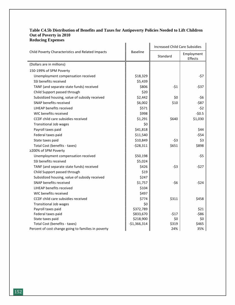
152
Table C4.5b Distribution of Benefits and Taxes for Antipoverty Policies Needed to Lift Children
Out of Poverty in 2010 Reducing Expenses
Child Poverty Characteristics and Related Impacts Baseline
Increased Child Care Subsidies
Standard Employment
Effects
(Dollars are in millions)
150-199% of SPM Poverty
Unemployment compensation received $18,329 -$7
SSI benefits received $5,439
TANF (and separate state funds) received $806 -$1 -$37
Child Support passed through $20
Subsidized housing, value of subsidy received $2,442 $0 -$6
SNAP benefits received $6,002 $10 -$87
LIHEAP benefits received $571 -$2
WIC benefits received $998 -$0.5
CCDF child care subsidies received $1,291 $640 $1,030
Transitional Job wages $0
Payroll taxes paid $41,818 $44
Federal taxes paid $11,540 -$54
State taxes paid $10,849 -$3 $3
Total Cost (benefits - taxes) -$28,311 $651 $898
≥200% of SPM Poverty
Unemployment compensation received $50,198 -$5
SSI benefits received $5,024
TANF (and separate state funds) received $426 -$3 -$27
Child Support passed through $19
Subsidized housing, value of subsidy received $247
SNAP benefits received $1,757 -$6 -$24
LIHEAP benefits received $104
WIC benefits received $497
CCDF child care subsidies received $774 $311 $458
Transitional Job wages $0
Payroll taxes paid $372,789 $21
Federal taxes paid $833,670 -$17 -$86
State taxes paid $218,900 $0 $0
Total Cost (benefits - taxes) -$1,366,314 $319 $465
Percent of cost change going to families in poverty 24% 35%
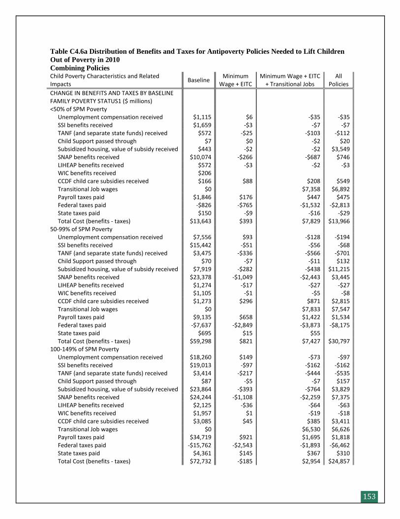
153
Table C4.6a Distribution of Benefits and Taxes for Antipoverty Policies Needed to Lift Children
Out of Poverty in 2010 Combining Policies Child Poverty Characteristics and Related Impacts
Baseline Minimum
Wage + EITC Minimum Wage + EITC
+ Transitional Jobs All
Policies
CHANGE IN BENEFITS AND TAXES BY BASELINE FAMILY POVERTY STATUS1 ($ millions) <50% of SPM Poverty Unemployment compensation received $1,115 $6 -$35 -$35 SSI benefits received $1,659 -$3 -$7 -$7 TANF (and separate state funds) received $572 -$25 -$103 -$112 Child Support passed through $7 $0 -$2 $20 Subsidized housing, value of subsidy received $443 -$2 -$2 $3,549 SNAP benefits received $10,074 -$266 -$687 $746 LIHEAP benefits received $572 -$3 -$2 -$3 WIC benefits received $206 CCDF child care subsidies received $166 $88 $208 $549 Transitional Job wages $0 $7,358 $6,892 Payroll taxes paid $1,846 $176 $447 $475 Federal taxes paid -$826 -$765 -$1,532 -$2,813 State taxes paid $150 -$9 -$16 -$29 Total Cost (benefits - taxes) $13,643 $393 $7,829 $13,966 50-99% of SPM Poverty Unemployment compensation received $7,556 $93 -$128 -$194 SSI benefits received $15,442 -$51 -$56 -$68 TANF (and separate state funds) received $3,475 -$336 -$566 -$701 Child Support passed through $70 -$7 -$11 $132 Subsidized housing, value of subsidy received $7,919 -$282 -$438 $11,215 SNAP benefits received $23,378 -$1,049 -$2,443 $3,445 LIHEAP benefits received $1,274 -$17 -$27 -$27 WIC benefits received $1,105 -$1 -$5 -$8 CCDF child care subsidies received $1,273 $296 $871 $2,815 Transitional Job wages $0 $7,833 $7,547 Payroll taxes paid $9,135 $658 $1,422 $1,534 Federal taxes paid -$7,637 -$2,849 -$3,873 -$8,175 State taxes paid $695 $15 $55 Total Cost (benefits - taxes) $59,298 $821 $7,427 $30,797 100-149% of SPM Poverty Unemployment compensation received $18,260 $149 -$73 -$97 SSI benefits received $19,013 -$97 -$162 -$162 TANF (and separate state funds) received $3,414 -$217 -$444 -$535 Child Support passed through $87 -$5 -$7 $157 Subsidized housing, value of subsidy received $23,864 -$393 -$764 $3,829 SNAP benefits received $24,244 -$1,108 -$2,259 $7,375 LIHEAP benefits received $2,125 -$36 -$64 -$63 WIC benefits received $1,957 $1 -$19 -$18 CCDF child care subsidies received $3,085 $45 $385 $3,411 Transitional Job wages $0 $6,530 $6,626 Payroll taxes paid $34,719 $921 $1,695 $1,818 Federal taxes paid -$15,762 -$2,543 -$1,893 -$6,462 State taxes paid $4,361 $145 $367 $310 Total Cost (benefits - taxes) $72,732 -$185 $2,954 $24,857
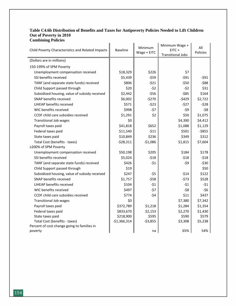
154
Table C4.6b Distribution of Benefits and Taxes for Antipoverty Policies Needed to Lift Children
Out of Poverty in 2010 Combining Policies
Child Poverty Characteristics and Related Impacts Baseline Minimum
Wage + EITC
Minimum Wage + EITC +
Transitional Jobs
All Policies
(Dollars are in millions)
150-199% of SPM Poverty
Unemployment compensation received $18,329 $226 $7
SSI benefits received $5,439 -$59 -$91 -$91
TANF (and separate state funds) received $806 -$21 -$50 -$88
Child Support passed through $20 -$2 -$2 $31
Subsidized housing, value of subsidy received $2,442 -$56 -$85 $164
SNAP benefits received $6,002 -$270 -$429 $2,722
LIHEAP benefits received $571 -$23 -$27 -$28
WIC benefits received $998 -$7 -$9 -$8
CCDF child care subsidies received $1,291 $2 $50 $1,075
Transitional Job wages $0 $4,390 $4,412
Payroll taxes paid $41,818 $652 $1,088 $1,129
Federal taxes paid $11,540 -$11 $501 -$855
State taxes paid $10,849 $236 $349 $312
Total Cost (benefits - taxes) -$28,311 -$1,086 $1,815 $7,604
≥200% of SPM Poverty
Unemployment compensation received $50,198 $205 $184 $178
SSI benefits received $5,024 -$18 -$18 -$18
TANF (and separate state funds) received $426 -$1 -$9 -$30
Child Support passed through $19 $50
Subsidized housing, value of subsidy received $247 -$5 -$14 $122
SNAP benefits received $1,757 -$58 -$73 $528
LIHEAP benefits received $104 -$1 -$1 -$1
WIC benefits received $497 -$7 -$8 -$6
CCDF child care subsidies received $774 -$4 $11 $437
Transitional Job wages $0 $7,380 $7,342
Payroll taxes paid $372,789 $1,218 $1,284 $1,354
Federal taxes paid $833,670 $2,153 $2,270 $1,430
State taxes paid $218,900 $595 $590 $579
Total Cost (benefits - taxes) -$1,366,314 -$3,855 $3,308 $5,238 Percent of cost change going to families in poverty na 65% 54%