Embed Size (px)
Citation preview
Reducing Capacity in U.S. Managed Fisheries An analysis of overcapacity and the cost of a vessel buyback program determined that substantial overcapacity existed in the New England and West Coast groundfish fisheries, the Atlantic swordfish and the large coastal shark fisheries, and the Gulf of Mexico shrimp fishery. James E. Kirkley, John M. Ward, James Nance, Frank Patella, Karyl Brewster-Geisz, Chris Rogers, Eric Thunberg, John Walden, Will Daspit, Brad Stenberg, Steve Freese, Jim Hastie, Stephen Holiman, and, Mike Travis
U.S. Department of Commerce National Oceanic and Atmospheric Administration National Marine Fisheries Service NOAA Technical Memorandum NMFS-F/SPO-76 November 2006

ii
iii
Reducing Capacity in U.S. Managed Fisheries An analysis of overcapacity and the cost of a vessel buyback program determined that substantial overcapacity existed in the New England and West Coast groundfish fisheries, the Atlantic swordfish and the large coastal shark fisheries, and the Gulf of Mexico shrimp fishery. James E. Kirkley, John M. Ward, James Nance, Frank Patella, Karyl Brewster-Geisz, Chris Rogers, Eric Thunberg, John Walden, Will Daspit, Brad Stenberg, Steve Freese, Jim Hastie, Stephen Holiman, and, Mike Travis NOAA Fisheries – Office of Sustainable Fisheries NOAA Technical Memorandum NMFS-F/SPO-76 November 2006
U.S. Department of Commerce Carlos M. Gutiérrez, Secretary National Oceanic and Atmospheric Administration Vice Admiral Conrad C. Lautenbacher, Jr., USN (Ret.) Under Secretary for Oceans and Atmosphere National Marine Fisheries Service William T. Hogarth, Assistant Administrator for Fisheries
iv
Suggested citation: Kirkley, James E., John M. Ward, James Nance, Frank Patella, Karyl Brewster-Geisz, Chris Rogers, Eric Thunberg, John Walden, Will Daspit, Brad Stenberg, Steve Freese, Jim Hastie, Stephen Holiman, and, Mike Travis. 2006. Reducing Capacity in U.S. Managed Fisheries. U.S. Dep. Commerce, NOAA Tech. Memo. NMFS-F/SPO-76, 45p.
A copy of this report may be obtained from: Office of Sustainable Fisheries NMFS, NOAA 1315 East-West Highway, F/SF8 Silver Spring, MD 20910 Or online at: http://spo.nmfs.noaa.gov/tm/index.htm
v
Reducing Capacity in U.S. Managed Fisheries
Contributing authors and researchers:
Editors: James E. Kirkley College of William and Mary School of Marine Science Virginia Institute of Marine Science Glouceter Point, VA John M. Ward Partnerships and Communications Division National Marine Fisheries Service Silver Spring, Maryland Contributing Authors and Researchers: Karyl Brewster-Geisz Chris Rogers Highly Migratory Species Management Division Office of Sustainable Fisheries National Marine Fisheries Service Silver Spring, Maryland Will Daspit Brad Stenberg Pacific States Marine Fisheries Commission Seattle, Washington Steve Freese Northwest Regional Office National Marine Fisheries Service Seattle, Washington Jim Hastie Northwest Fisheries Science Center National Marine Fisheries Service Seattle, Washington Stephen Holiman Mike Travis Southeast Regional Office National Marine Fisheries Service St. Petersburg, Florida
James E. Kirkley College of William and Mary School of Marine Science Virginia Institute of Marine Science Glouceter Point, VA James Nance Frank Patella Galveston Laboratory Southeast Fisheries Science Center National Marine Fisheries Service Galveston, Texas Eric Thunberg John Walden Social Sciences Branch Northeast Fisheries Science Center National Marine Fisheries Service Woods Hole, Massachusetts John M. Ward Partnerships and Communications Division Office of Sustainable Fisheries National Marine Fisheries Service Silver Spring, Maryland
Reducing Capacity in U.S. Managed Fisheries Executive Summary
vi
Executive Summary
NOAA Fisheries (the National Marine Fisheries Service), the Food and Agriculture Organization (FAO), and numerous member nations have long been concerned about the presence of excess and overcapacity in commercial fisheries. Simply, fishing fleets around the world have the capability to harvest well in excess of desired and sustainable levels. More important, the presence of excess and overcapacity typically cause substantial economic waste in the form of higher than necessary costs of production, reduced net benefits to society, and biological overfishing. NOAA and various nations, along with the FAO, are, therefore, seeking ways to globally rationalize fleet sizes.
There are, however, numerous aspects related to the concept of capacity, which have
not been fully examined, particularly relative to promoting the sustainable use of marine resources. There is the issue of excess capacity vs. overcapacity (Ward, Thunberg, and Mace, 2005). The concept of capacity is, in general, a short-run concept. It is a measure of the potential maximum output that could be produced given the fixed factors (e.g., capital stock, vessel and engine size, gear, and equipment), full-utilization of the variable factors of production (e.g., labor, fuel, and days at sea), and customary and usual operating procedures (CUOP). Excess capacity generally pertains to the difference between the potential output, which could be produced, and the actual output, which was produced, given existing resource conditions, the fixed factors of production, and operating subject to customary and usual operating procedures. For example, an existing fishing fleet might only be capable of catching and landing 10.0 million pounds of fish, given existing resource conditions. If resource conditions improved, however, the fleet might well be able to catch and land considerably more than 10.0 million pounds. And if resource levels were restored to desired target or maximum sustainable yield (MSY) levels, an existing fleet may or may not have too much harvesting capacity. For this latter case, the concept of capacity is referred to as overcapacity, which is the maximum potential output a fleet could realize, given fixed factors of production, desired or target levels of resources, full-utilization of the variable inputs, and operating under customary and usual operating procedures. Another issue, which is of extreme importance relative to rationalizing fleet size, is how to reduce capacity in fisheries.
NOAA Fisheries has become particularly concerned about the overcapacity in
America’s commercial fishing industry, and the reduction in fleet size necessary to make it commensurate with sustainable resource levels. In response to this concern, Bill Hogarth, Assistant Administrator (AA) of NOAA Fisheries, has provided this report on the nature of overcapacity and the cost of reducing overcapacity in federally managed fisheries. In addition, an analysis of overcapacity and the cost of a vessel buyback program to reduce overcapacity in five federally managed fisheries was undertaken by NOAA economists and academic researchers. The five fisheries examined were the New England and West Coast groundfish fisheries, the Atlantic swordfish fishery, the Atlantic large coastal shark fishery, and the Gulf of Mexico shrimp fishery. All five fisheries were determined to have substantial overcapacity, with the more severe level of overcapacity occurring in the west-coast groundfish fishery.
Reducing Capacity in U.S. Managed Fisheries Executive Summary
vii
Vessel reductions necessary for eliminating overcapacity were as follows: (1) New England groundfish—588 vessels and 725 latent permits; (2) Gulf of Mexico shrimp fishery—875 vessels; (3) Atlantic swordfish fishery—86 vessels; (4) Atlantic large coastal sharks—206 vessels; and (5) West Coast groundfish fishery—1,260 vessels. The estimated costs of reducing capacity, through the use of a buyback program, for each of the five fisheries were as follows: (1) New England groundfish—$460.7 million; (2) Gulf of Mexico shrimp fishery—$329.9 million; (3) Atlantic swordfish fishery—$25.7 million; (4) Atlantic large coastal sharks—$34.0 million; and (5) West Coast groundfish fishery—$149.3 million. The total cost of reducing overcapacity was estimated to equal approximately $1.0 billion (2002 constant dollars).
This report provides a summary and overview of the methodology used to estimate
capacity and the cost of reducing capacity. It also provides a description of the data and sources of data used to estimate overcapacity in the five fisheries. Last, it provides estimates of overcapacity and the cost of reducing overcapacity for each of the five fisheries.
NOAA Fisheries—2006 Reducing Capacity in U.S. Managed Fisheries
viii
Table of Contents
Section Page Executive Summary ........................................................................................................ vi 1.0 Introduction ............................................................................................................... 1 2.0 Concepts, Methodology, Assumptions, and Data ................................................... 3
2.1 Definitions and Concepts of Capacity ................................................................... 3 2.2.2 Primal and Economic Measures of Capacity .................................................. 3
2.2 Methods for Estimating Capacity Output .............................................................. 9 2.2.1 Data Envelopment Analysis and Capacity...................................................... 9 2.2.2 Capacity Utilization and DEA ...................................................................... 12
2.3 Assumptions for Estimating Capacity and Capacity Utilization .......................... 13 2.4 Estimating the Costs To Support a Buyback ........................................................ 14 2.5 Overcapacity and Target Levels ........................................................................... 15 2.6 The Fisheries and Data ......................................................................................... 16
2.6.1 The New England Groundfish Fishery ......................................................... 16 2.6.2 The West Coast Groundfish Fishery............................................................. 17 2.6.3 The Gulf of Mexico Shrimp Fishery............................................................. 17 2.6.4 The Atlantic Swordfish Fishery.................................................................... 18 2.6.5 The Large Coastal Pelagic Shark Fishery..................................................... 18
3.0 Estimates of Capacity.............................................................................................. 20 3.1 The New England Groundfish Fishery ................................................................. 20 3.2 The West Coast Groundfish Fishery .................................................................... 25 3.3 The Gulf of Mexico Shrimp Fishery .................................................................... 27 3.6 Overview of Overcapacity and the Cost of a Buyback Program .......................... 40
4.0 Summary and Conclusions ..................................................................................... 41 References ....................................................................................................................... 43
NOAA Fisheries—2006 Reducing Capacity in U.S. Managed Fisheries
ix
List of Tables Table Page Table 1. Estimated Capacity Output and the Full-utilization Days at Sea for the Three Georges Bank Fisheries.................................................................................................... 22 Table 2. Estimated Capacity Output and the Full-utilization Days at Sea for the Three Gulf of Maine Fisheries ................................................................................................... 22 Table 3. Estimated Capacity Output and the Full-utilization Days at Sea for the Combined Georges Bank and Gulf of Maine Fisheries.................................................... 22 Table 4. Estimates of Overcapacity and the Costs of Reducing Overcapacity in the Georges Bank/Gulf of Maine Fishery .............................................................................. 23 Table 5. Overcapacity, Estimated Reduction in Fleet Size, and Estimated Cost of Buyback Program to Reduce Capacity in Five Federally-Managed Fisheries ................. 24 Table 6. Estimates of Capacity in the West Coast Groundfish Fishery........................... 26 Table 7. Overcapacity and Estimated Cost of Reducing Overcapacity in the West Coast Groundfish Fisherya ......................................................................................................... 27 Table 8. Estimates of Capacity Output for Area 5 and Five Corresponding Depth Zones, Gulf of Mexico Shrimp Fishery ....................................................................................... 28 Table 9. Estimates of Capacity Output for Area 4 and Five Corresponding Depth Zones, Gulf of Mexico Shrimp Fishery ....................................................................................... 29 Table 10. Estimates of Capacity Output for Area 3 and Five Corresponding Depth Zones, Gulf of Mexico Shrimp Fishery ....................................................................................... 30 Table 11. Estimates of Capacity Output for Area 2 and Five Corresponding Depth Zones, Gulf of Mexico Shrimp Fishery ....................................................................................... 31 Table 12. Estimates of Capacity Output for Area 1 and Five Corresponding Depth Zones, Gulf of Mexico Shrimp Fishery ....................................................................................... 32 Table 14. Maximum Average Annual Days per Year per Vessel and Year of Maximum In the Gulf of Mexico Shark Fishery................................................................................ 34 Table 15. Capacity Output for the U.S. North and South Atlantic Swordfish Fisheries . 36 Table 17. Summary Information for the Large Coastal Pelagic Shark Fishery............... 38 Table 18. Capacity Output and Cost of Buyback Program for the Large Coastal Pelagic Shark Fishery ................................................................................................................... 39

NOAA Fisheries—2006 Reducing Capacity in U.S. Managed Fisheries
x
List of Figures Figure Page Figure 1. Economic-based concepts of Capacity .............................................................. 5 Figure 2. The Production Frontier and Capacity Output ................................................... 6 Figure 3. Sustainable Yield Curve and Overcapacity........................................................ 8 Figure 4. Input and Output-Oriented Measures of Technical Efficiency ........................ 11
Reducing Capacity in U.S. Managed Fisheries Introduction
1
1.0 Introduction U.S. fishery managers and administrators widely recognize that many fisheries of the
United States suffer from either severe excess or overcapacity. That is, fishing fleets have the capability to harvest well in excess of levels actually being harvested or levels that can be sustained. The consequences of this excess harvesting capacity are typically severe biological overfishing; substantial economic waste in the form of higher production costs and reduced earnings for vessels and the fleet; and increasingly restrictive management that can be quite costly in terms of expenditures required to support management and regulation. The concept of capacity, however, is often vague and sometimes ambiguous. It is often confused with the concept of capitalization, which refers to the level of the capital stock (Berndt and Fuss, 1989). To some, the concept equates to an output level, and to others, it may imply the productive capability (e.g., a fishing vessel, fuel, and labor utilization), or the input set required to produce a given level of output. The National Marine Fisheries Service (NMFS) and the Food and Agriculture Organization (FAO) have developed what appears to be a reasonable and increasingly accepted definition of capacity; it is the amount of fish (or fishing effort) that can be produced over a given period of time (e.g., a year or a fishing season) by a vessel or fleet if fully utilized and for a given resource condition.
NMFS has, however, extended the concept of capacity to distinguish excess capacity from overcapacity (Ward, Thunberg, and Mace, 2005). While seemingly trivial, the distinction is an important one. Excess explicitly refers to a short-run phenomenon, which is likely to be self-correcting; overcapacity, however, refers to a more long-term phenomenon that is likely to be persistent and of indefinite duration. Alternatively, the concept—overcapacity—explicitly recognizes the possibility that a given fleet could utilize its variable and fixed inputs so as to have the capability to harvest well in excess of a desired target level of production (e.g., maximum sustainable yield, MSY).
Economists have generally suggested that the problem of overcapacity can be addressed through the introduction of individual transferable quotas or other quasi-private property rights’ regimes (see, for example, Grafton et al. 1996 and Squires et al. 1995). An alternative approach for reducing capacity is to implement buyback programs. A buyback offers one way to quickly reduce capacity to help facilitate the rebuilding of fish stocks. Under a buyback program, industry, the government, or a collaborative industry/government structure agrees to purchase commercial fishing vessels. Albeit the National Marine Fisheries Service has a formal set of guidelines, which must be followed to implement a buyback program, considerable concern exists about the financial cost of a buyback program. As a result, Bill Hogarth, the Assistant Administrator (AA) for Fisheries, requested in May of 2002 that estimates of overcapacity and the direct financial cost of reducing overcapacity in federally managed fisheries be provided. Five federally managed fisheries were chosen including the New England and West Coast groundfish fisheries, Atlantic swordfish fishery, the Atlantic large coastal shark fishery, and the Gulf of Mexico shrimp fishery.

Reducing Capacity in U.S. Managed Fisheries Introduction
2
This report provides estimates of overcapacity and the cost of reducing overcapacity in the five fisheries. It is noted, however, that the estimates are preliminary or a first-round approximation of the level of overcapacity and cost of reducing overcapacity in the five fisheries. More precise estimates are anticipated to be available in the future as additional and more extensive information, particularly detailed economic data, becomes available. The next section provides an overview of the concept of capacity; methodology used to assess capacity and estimate the cost of reducing overcapacity; the assumptions required to estimate capacity and the cost of overcapacity; and the source and integrity of available data. Section 3 presents the empirical estimates of overcapacity, the number of vessels and costs required to eliminate overcapacity. Section 4 provides the summary and conclusions.
Reducing Capacity in U.S. Managed Fisheries Concepts, Methodology, and Data
3
2.0 Concepts, Methodology, Assumptions, and Data
Estimation of capacity and the cost of reducing overcapacity require a methodology, assumptions, and data. Prior to presenting a discussion about the methodology, however, the basic concept of capacity needs to be defined and presented. 2.1 Definitions and Concepts of Capacity
The concept of capacity is often vague and confusing to individuals, particularly to non-economists. In its widest usage, capacity refers to the maximum output that can be produced, given full utilization of the variable inputs (i.e., utilization of inputs that can be varied and are used such that maximum possible production is realized), the limitations of the fixed factors (i.e., those factors that cannot be easily changed, such as the size of plant or fishing vessel), customary and usual operating procedures, and output and input prices. NOAA Fisheries, following the definition offered by FAO, defines capacity as the level of output a firm is able, or willing and able, to produce given specified conditions and constraints (NMFS, 2001). As such, both the general and NMFS concepts of capacity are output-based or output-oriented. That is, capacity is defined and measured in terms of output levels.
In contrast, the notion of an input-based or input oriented measure of capacity has
been offered (Kirkley and Squires, 1999). This concept, however, is not consistent with the basic notion of capacity. The input-oriented measure attempts to define capacity in terms of the minimum level of variable and fixed factors required to produce a given output. As such, it is inconsistent with the concept of capacity, which is primarily a short-run notion. An alternative input-based measure, which is actually derived from an output-oriented concept, is the level of fixed factors required to produce the maximum output, given full-utilization of the variable inputs. For example, assume that 20 fishing vessels could harvest 100,000 mt of product a year, given full utilization of the variable inputs, but were only producing 50,000 mt per year. Only 10 vessels would then be necessary to harvest the 50,000 mt per year. The fleet of 20 vessels would, thus, have too much harvesting capacity. It is this latter notion of capacity that is of increasing concern to NOAA Fisheries because it facilitates the determination of the number of vessels and their level of operation necessary to harvest a stated target level of catch. 2.2.2 Primal and Economic Measures of Capacity
Although the preferred measure of capacity is a measure based on economic decision-making behavior (i.e., an economic-based measure of capacity), which reflects capacity output and input levels consistent with economic optimizing behavior, data necessary for estimating the economic concept of capacity are not available for many fisheries of the United States (Kirkley et al. 2001; NMFS 2001). This is particularly the case for the five fisheries examined in this study. For the purposes of this study, it was decided to estimate the “primal” or “technological-economic” concept of capacity. The technological-economic concept is a physical measure of the capacity output, which although having no explicit economic motivations, does implicitly recognize that observed behavior is reflected in the empirical observations. This measure of capacity
Reducing Capacity in U.S. Managed Fisheries Concepts, Methodology, and Data
4
provides a physical measure of capacity output that reflects economic decision-making behavior, but cannot be used to predict capacity output in response to changes in behavior or input and output prices. 2.1.1.1 Economic-based Measures of Capacity
The basic concept of capacity is an economic concept. Formally, it is defined as the level of output corresponding to a tangency between the short and long-run average cost curves. It is formally a short-run concept, because in the long-run, it is possible to change the levels of fixed factors, and thus, change the level of capacity. Capacity may also be defined according to output levels corresponding to maximum revenue or maximum profit (F@re et al. 2000; Coelli et al. 2001). Concepts of capacity based on economic optimizing behavior are referred to as economic-based measures of capacity.
For the case of fisheries, however, economic data are seldom available, and thus,
capacity can usually only be estimated using data on physical quantities of inputs and outputs. Kirkley and Squires (1999) refer to this concept as the “technological-economic” concept of capacity. This is because the empirical data reflect decision-makers responses to changes in economic conditions, but the analysis cannot accommodate changes in economic conditions.
Coelli et al. provide a comparison of capacity output based on economic and
technological-economic concepts. Coelli et al. discuss four possible concepts of capacity; three of which were economic-based concepts, and one was the Johansen (1968) concept. Two concepts, Klein (1960) and Berndt and Morrison (1981), were based on short-run cost functions. Klein defined capacity output to be that output (K) at which the short-run average cost curve equals or is tangent to the long-run average cost curve (Figure 1).1 Berndt and Morrison defined capacity output (BM) as that level of output corresponding to the tangency between the minimum short-run average cost and the long-run average cost. Given constant returns to scale, where a given percentage increase in all input causes the same percentage increase in output, the concepts of Klein and Berndt and Morrison are identical. The Johansen concept of capacity output (J) equals the maximum potential output that could be produced given fixed factors and unrestricted levels of variable inputs. Coelli et al., however, argued that defining capacity output (CGP) based only on the tangency of short and long-run average cost curves completely ignores the possibility of firms earning negative profits, and that producers would not normally continue to operate at a loss. Coelli et al. argue, subsequently, that capacity output is the level of output necessary to maximize profits.
1 The short-run cost curve is the cost curve corresponding to a period during which some factors of production cannot be changed. In the long-run, it is assumed that all factors of production may be changed.

Reducing Capacity in U.S. Managed Fisheries Concepts, Methodology, and Data
5
Figure 1. Economic-based concepts of Capacity
In Figure 1, K stands for Klein’s level of capacity output; BM indicates Berndt and Morrison’s concept; and CGP indicates Coelli et al.’s measure; P indicates price; MC indicates marginal cost; and SR and LR indicate short and long-run. Johansen’s concept occurs at the far right of the short-run average cost curve. 2.1.1.2 The Technological-Economic Concept of Capacity
In the estimation and analysis of capacity in fisheries, it is usually necessary to consider the technological-economic concept; this is simply because input prices and costs data are typically not available. One technological-economic measure of capacity output is the maximum potential output that could be produced if a firm or fishing vessel operated efficiently and was not constrained by the availability of variable factors of production (e.g., fuel and labor). This is the traditional Johansen (1968) concept of capacity output. The technological-economic measure of capacity output used in this study is a weak variant of the concept (F@re 1984). The weaker concept permits a fixed factor (e.g., vessel size or level of capital) to limit or constrain output.
To better understand the concept of capacity output, consider Figure 2, which depicts
a production frontier. The production frontier or technology depicts the maximum output that can be produced given fixed and variable inputs. Points on the frontier represent technically efficient production, and points below the frontier depict inefficient production. The vertical axis, Y, indicates output levels, and the horizontal axis, K,
Reducing Capacity in U.S. Managed Fisheries Concepts, Methodology, and Data
6
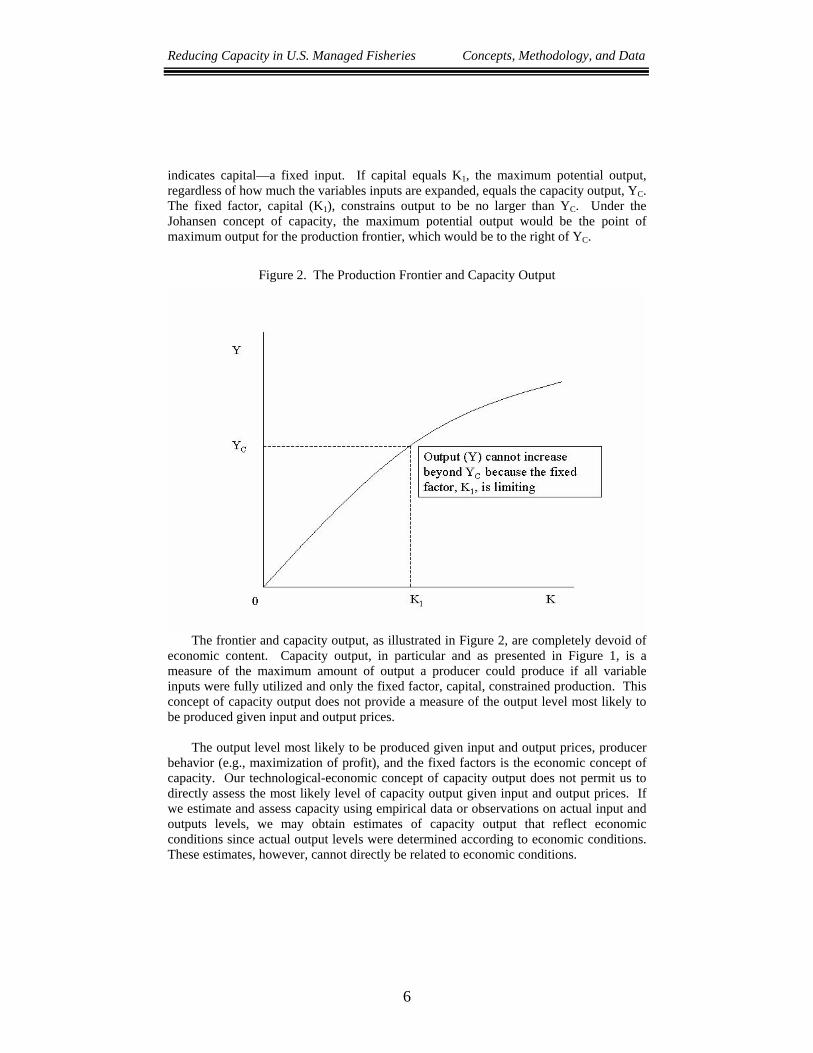
indicates capital—a fixed input. If capital equals K1, the maximum potential output, regardless of how much the variables inputs are expanded, equals the capacity output, YC. The fixed factor, capital (K1), constrains output to be no larger than YC. Under the Johansen concept of capacity, the maximum potential output would be the point of maximum output for the production frontier, which would be to the right of YC.
Figure 2. The Production Frontier and Capacity Output
The frontier and capacity output, as illustrated in Figure 2, are completely devoid of
economic content. Capacity output, in particular and as presented in Figure 1, is a measure of the maximum amount of output a producer could produce if all variable inputs were fully utilized and only the fixed factor, capital, constrained production. This concept of capacity output does not provide a measure of the output level most likely to be produced given input and output prices.
The output level most likely to be produced given input and output prices, producer
behavior (e.g., maximization of profit), and the fixed factors is the economic concept of capacity. Our technological-economic concept of capacity output does not permit us to directly assess the most likely level of capacity output given input and output prices. If we estimate and assess capacity using empirical data or observations on actual input and outputs levels, we may obtain estimates of capacity output that reflect economic conditions since actual output levels were determined according to economic conditions. These estimates, however, cannot directly be related to economic conditions.
Reducing Capacity in U.S. Managed Fisheries Concepts, Methodology, and Data
7
2.1.1.3 Overcapacity in Fisheries
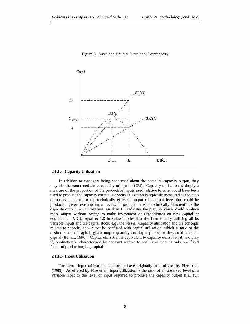
A major concern of the National Marine Fisheries Service (NMFS) is whether or not fishing fleets would have overcapacity if resource levels were fully restored to their desired optimum or target levels; e.g., maximum sustainable yield (MSY) biomass. Many of the nation’s fishery resources are at stock abundance levels below those necessary to sustain MSY harvests. Alternatively, some fisheries have resources that are fully utilized and are at levels consistent with desired levels, but fishing must be heavily regulated to prevent resource declines and associated problems. This latter situation characterizes wasted resources and lower than possible levels of economic productivity. For those fishery resources with levels less than those considered to be optimum, production is lower than it would be if resources were at desired levels. Alternatively, our production technology (i.e., the technology that describes the relationship between outputs and inputs) yields output levels for a given level of fishing effort that is lower than it would be with more abundant resource levels. The case of overcapacity is, then, the potential maximum output that could be produced if resources were at their desired levels less the target level of landings (e.g., a MSY level of landings). Using the surplus production framework of Schaefer (1954), the concept of overcapacity may be illustrated. Consider Figure 3, which depicts sustainable levels of landings for a fishing fleet given different levels of fishing effort. Points on the sustainable yield curve represent levels of landings corresponding to different levels of the resource, and for which additions to the stock equal removals. The maximum point represents maximum sustainable yield (MSY); the MSY is the maximum average yield that can be harvested for a given time period, usually per year. The origin of the sustainable yield curves corresponds to the maximum population, which is also referred to as the environmental carrying capacity (EEC).
Catch is on the vertical axis in Figure 3, and fishing effort (a measure of total inputs expended to harvest fish) is depicted on the horizontal axis. The maximum sustainable yield catch occurs for EMSY in Figure 3. A short-run yield (SRYC) or catch-effort function of the form C = q E N, where C is catch, q is the catchability coefficient, E is fishing effort, and population size (N) is imposed on the sustainable yield curve. For the short-run yield function in Figure 3, N is the population corresponding to maximum sustainable yield. If the fleet exerted EMSY units of effort, the MSY level of catch would be harvested. As depicted in Figure 3, however, the fleet has the capability to harvest in excess of MSY in the short-run; in this case, the fleet has overcapacity because they could increase their fishing effort to EC and harvest in excess of the MSY (CMSY) level. The amount of overcapacity is CC – CMSY. Now consider a decline in resource conditions, such that the short-run yield function shifts downward to SRYC1. If the difference between CC and CO, the observed catch, is considered, there is excess capacity, which equals CC – CO. Observe, however, that the observed catch (Co) could have been below the MSY level, and thus, the excess capacity would be more than overcapacity. The major distinction between the two—over and excess capacity—is the time horizon and the reference to a target or desired level of catch (e.g., MSY).
Reducing Capacity in U.S. Managed Fisheries Concepts, Methodology, and Data
8
Figure 3. Sustainable Yield Curve and Overcapacity
2.1.1.4 Capacity Utilization
In addition to managers being concerned about the potential capacity output, they may also be concerned about capacity utilization (CU). Capacity utilization is simply a measure of the proportion of the productive inputs used relative to what could have been used to produce the capacity output. Capacity utilization is typically measured as the ratio of observed output or the technically efficient output (the output level that could be produced, given existing input levels, if production was technically efficient) to the capacity output. A CU measure less than 1.0 indicates the plant or vessel could produce more output without having to make investment or expenditures on new capital or equipment. A CU equal to 1.0 in value implies that the firm is fully utilizing all its variable inputs and the capital stock; e.g., the vessel. Capacity utilization and the concepts related to capacity should not be confused with capital utilization, which is ratio of the desired stock of capital, given output quantity and input prices, to the actual stock of capital (Berndt, 1990). Capital utilization is equivalent to capacity utilization if, and only if, production is characterized by constant returns to scale and there is only one fixed factor of production; i.e., capital.
2.1.1.5 Input Utilization
The term—input utilization—appears to have originally been offered by F@re et al. (1989). As offered by F@re et al., input utilization is the ratio of an observed level of a variable input to the level of input required to produce the capacity output (i.e., full
Reducing Capacity in U.S. Managed Fisheries Concepts, Methodology, and Data
9
utilization). If input utilization is less than 1.0 in value, it implies that producers are using fewer variable inputs than necessary to produce the capacity output; if the ratio is greater than 1.0, producers have a surplus of variable inputs (i.e., they are using too much of a variable input). F@re et al. (1994) also offer an inverse measure of input utilization, which equals the ratio of the variable inputs required to produce the capacity output to the variable inputs actually used to produce a given output level. 2.2 Methods for Estimating Capacity Output There are numerous methods for empirically estimating capacity output. A detailed description of the various methods is presented in Kirkley and Squires (1999a), NMFS (2001), and Kirkley et al. (2001, 2002). Briefly, there are five basic methods, which may be used to estimate capacity. One approach is to conduct a survey as done by Census for the Federal Reserve. In the survey, plant managers are asked to provide information about the maximum potential output given customary and usual operating procedures. Another approach is to specify a dual cost function when economic data are available, and determine the output level corresponding to short and long-run average costs being equal. A third approach is the stochastic production frontier. With this approach, a production function is estimated and evaluated at levels of the inputs needed to impute the potential output that would be possible with combinations of the fixed and variable factors; this approach is described more thoroughly in Kirkley et al. (2002). Another approach is the peak to peak approach of Klein and Long (1973). With the peak to peak approach, aggregate output levels are divided by number of firms over time; peak levels of output per unit input are identified; and these are interpreted as capacity output levels. Typically, the output per unit input levels between the peak levels are adjusted for technical change and used to estimate capacity for all periods. Ballard and Roberts (1977) used the Klein approach to estimate capacity output in ten U.S. fisheries. The approach used in this study is to use data envelopment analysis (DEA) to estimate the concept of capacity output offered by F@re (1984). Since DEA was the method used to estimate capacity output in the five U.S. managed fisheries, we restrict our methodological discussion to DEA; detailed discussions of the other methods are provided in Klein (1960), Berndt and Morrison (1981), Morrison (1985a,b), Segerson and Squires (1990, 1993, and 1995), Kirkley and Squires (1999a,b), and Coelli et al. (2001). 2.2.1 Data Envelopment Analysis and Capacity Data envelopment analysis (DEA) is a non-parametric, non-statistical approach for determining technical and economic efficiency. That is, no parameters, as in regression, are directly estimated, and no statistical distributions are assumed. It is based on mathematical programming. Charnes et al. (1978) offered the method as an approach for assessing the efficiency of decision-making units. The basic premise upon which DEA operates is the mathematical distance function. More recent work, however, is focusing on the use of directional distance vectors, which permit consideration of undesirable outputs (e.g., bycatch) and both expansions and contractions of, respectively, outputs and inputs. For the purposes of this report, however, we restrict attention to the conventional DEA framework, which uses distance functions.
Reducing Capacity in U.S. Managed Fisheries Concepts, Methodology, and Data
10
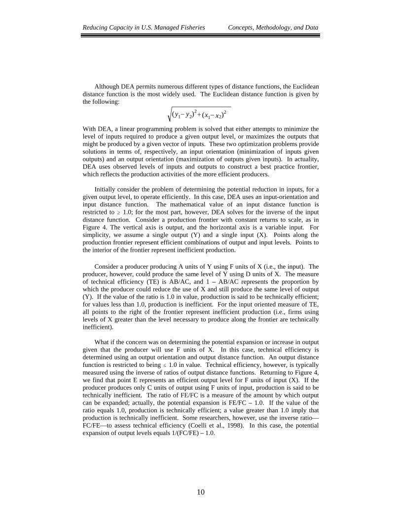
Although DEA permits numerous different types of distance functions, the Euclidean distance function is the most widely used. The Euclidean distance function is given by the following:
21 2
21 2( ) ( )y y x x− + −
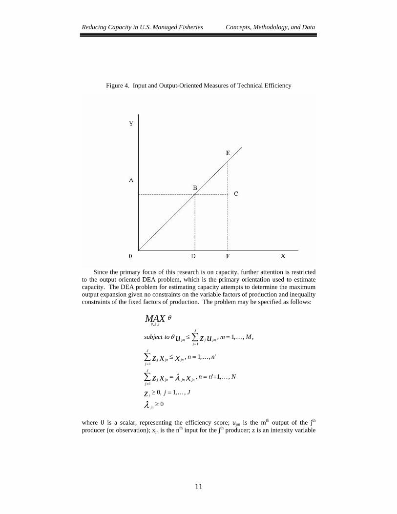
With DEA, a linear programming problem is solved that either attempts to minimize the level of inputs required to produce a given output level, or maximizes the outputs that might be produced by a given vector of inputs. These two optimization problems provide solutions in terms of, respectively, an input orientation (minimization of inputs given outputs) and an output orientation (maximization of outputs given inputs). In actuality, DEA uses observed levels of inputs and outputs to construct a best practice frontier, which reflects the production activities of the more efficient producers. Initially consider the problem of determining the potential reduction in inputs, for a given output level, to operate efficiently. In this case, DEA uses an input-orientation and input distance function. The mathematical value of an input distance function is restricted to $ 1.0; for the most part, however, DEA solves for the inverse of the input distance function. Consider a production frontier with constant returns to scale, as in Figure 4. The vertical axis is output, and the horizontal axis is a variable input. For simplicity, we assume a single output (Y) and a single input (X). Points along the production frontier represent efficient combinations of output and input levels. Points to the interior of the frontier represent inefficient production.
Consider a producer producing A units of Y using F units of X (i.e., the input). The producer, however, could produce the same level of Y using D units of X. The measure of technical efficiency (TE) is AB/AC, and 1 – AB/AC represents the proportion by which the producer could reduce the use of X and still produce the same level of output (Y). If the value of the ratio is 1.0 in value, production is said to be technically efficient; for values less than 1.0, production is inefficient. For the input oriented measure of TE, all points to the right of the frontier represent inefficient production (i.e., firms using levels of X greater than the level necessary to produce along the frontier are technically inefficient).
What if the concern was on determining the potential expansion or increase in output
given that the producer will use F units of X. In this case, technical efficiency is determined using an output orientation and output distance function. An output distance function is restricted to being # 1.0 in value. Technical efficiency, however, is typically measured using the inverse of ratios of output distance functions. Returning to Figure 4, we find that point E represents an efficient output level for F units of input (X). If the producer produces only C units of output using F units of input, production is said to be technically inefficient. The ratio of FE/FC is a measure of the amount by which output can be expanded; actually, the potential expansion is FE/FC – 1.0. If the value of the ratio equals 1.0, production is technically efficient; a value greater than 1.0 imply that production is technically inefficient. Some researchers, however, use the inverse ratio—FC/FE—to assess technical efficiency (Coelli et al., 1998). In this case, the potential expansion of output levels equals 1/(FC/FE) – 1.0.
Reducing Capacity in U.S. Managed Fisheries Concepts, Methodology, and Data
11
Figure 4. Input and Output-Oriented Measures of Technical Efficiency
Since the primary focus of this research is on capacity, further attention is restricted
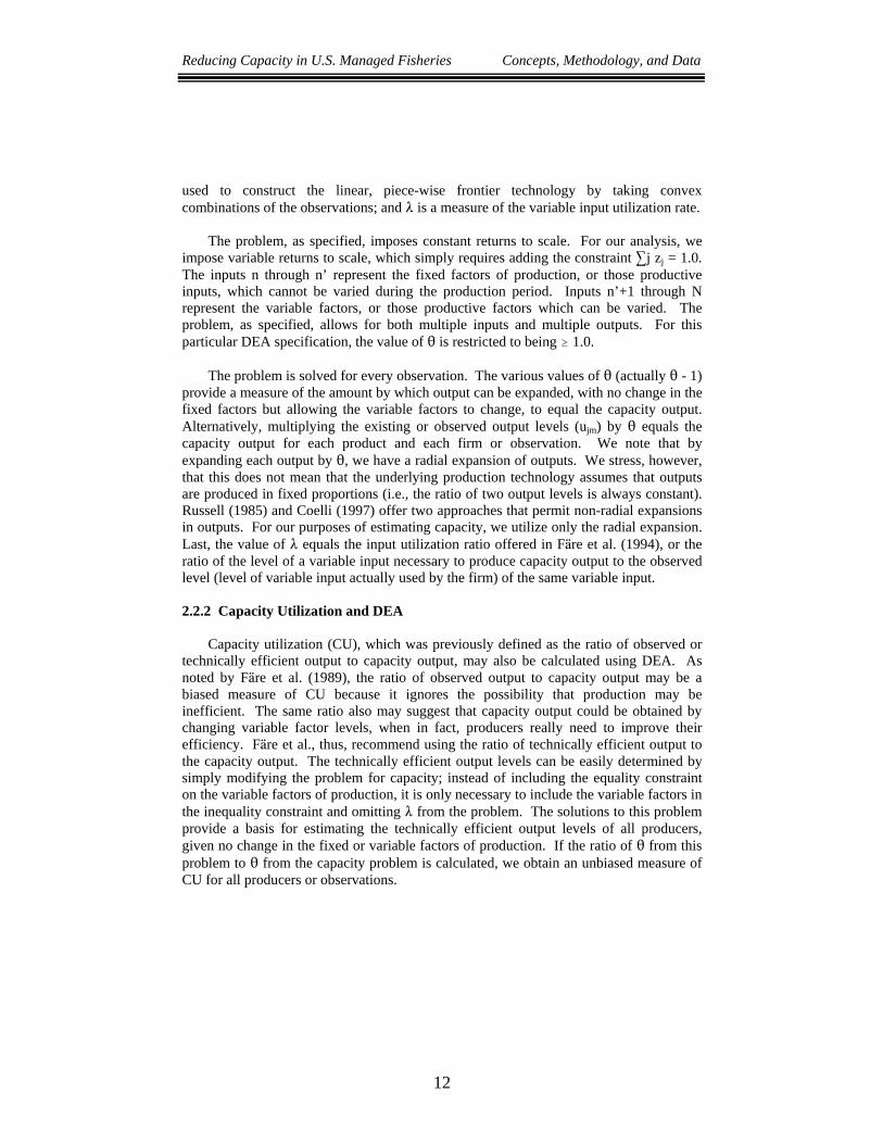
to the output oriented DEA problem, which is the primary orientation used to estimate capacity. The DEA problem for estimating capacity attempts to determine the maximum output expansion given no constraints on the variable factors of production and inequality constraints of the fixed factors of production. The problem may be specified as follows:
θ λθ
θ
λ
λ
, ,
, , ... , ,
, , ... , '
, ' , ... ,
, , ... ,
z
jm jj
J
jm
jj
J
jn jn
jj
J
jn jn jn
j
jn
MAX
u z u
z x x
z x xz
subject to m M
n n
n n N
j J
≤ =
≤ =
= = +
≥ =
≥
=
=
=
∑
∑
∑
1
1
1
1
1
1
0 1
0
where 2 is a scalar, representing the efficiency score; ujm is the mth output of the jth producer (or observation); xjn is the nth input for the jth producer; z is an intensity variable
Reducing Capacity in U.S. Managed Fisheries Concepts, Methodology, and Data
12
used to construct the linear, piece-wise frontier technology by taking convex combinations of the observations; and 8 is a measure of the variable input utilization rate.
The problem, as specified, imposes constant returns to scale. For our analysis, we
impose variable returns to scale, which simply requires adding the constraint 3j zj = 1.0. The inputs n through n’ represent the fixed factors of production, or those productive inputs, which cannot be varied during the production period. Inputs n’+1 through N represent the variable factors, or those productive factors which can be varied. The problem, as specified, allows for both multiple inputs and multiple outputs. For this particular DEA specification, the value of 2 is restricted to being $ 1.0. The problem is solved for every observation. The various values of 2 (actually 2 - 1) provide a measure of the amount by which output can be expanded, with no change in the fixed factors but allowing the variable factors to change, to equal the capacity output. Alternatively, multiplying the existing or observed output levels (ujm) by 2 equals the capacity output for each product and each firm or observation. We note that by expanding each output by 2, we have a radial expansion of outputs. We stress, however, that this does not mean that the underlying production technology assumes that outputs are produced in fixed proportions (i.e., the ratio of two output levels is always constant). Russell (1985) and Coelli (1997) offer two approaches that permit non-radial expansions in outputs. For our purposes of estimating capacity, we utilize only the radial expansion. Last, the value of 8 equals the input utilization ratio offered in F@re et al. (1994), or the ratio of the level of a variable input necessary to produce capacity output to the observed level (level of variable input actually used by the firm) of the same variable input. 2.2.2 Capacity Utilization and DEA Capacity utilization (CU), which was previously defined as the ratio of observed or technically efficient output to capacity output, may also be calculated using DEA. As noted by F@re et al. (1989), the ratio of observed output to capacity output may be a biased measure of CU because it ignores the possibility that production may be inefficient. The same ratio also may suggest that capacity output could be obtained by changing variable factor levels, when in fact, producers really need to improve their efficiency. F@re et al., thus, recommend using the ratio of technically efficient output to the capacity output. The technically efficient output levels can be easily determined by simply modifying the problem for capacity; instead of including the equality constraint on the variable factors of production, it is only necessary to include the variable factors in the inequality constraint and omitting 8 from the problem. The solutions to this problem provide a basis for estimating the technically efficient output levels of all producers, given no change in the fixed or variable factors of production. If the ratio of 2 from this problem to 2 from the capacity problem is calculated, we obtain an unbiased measure of CU for all producers or observations.
Reducing Capacity in U.S. Managed Fisheries Concepts, Methodology, and Data
13
2.3 Assumptions for Estimating Capacity and Capacity Utilization
The National Marine Fisheries Service (NOAA Fisheries) desired to have estimates of capacity output, conditional on the assumption that resource levels were fully restored to desired targets. That is, what would be the maximum potential output, given customary and usual operating procedures, and resource levels at the desired targets? This is not an easy question to ask. First, available data do not reflect fishing observations during periods when fisheries were not heavily regulated or periods during which the resources were at desired target levels. Second, it cannot be easily ascertained how fishers would change their fishing strategies and input levels if resources were fully restored. Third, there is no information available to assess how production responses would change in response to fully restored resource levels.
As an example, lets modify the very simple catch-effort relationship considered
earlier. Specifically, lets give the production technology the form C = q E" K$ N', where as before C is catch, q is the catchability coefficient, E is a variable input—fishing effort, K is a fixed factor, and N is the resource condition. However, the added coefficients for each of the variables now provides a measure of the production response to changes in the levels of each input; formerly, these are referred to as output elasticities because they indicate the percentage change in output for a one-percent change in each input, including N. The output elasticities are assumed to be positive in value. Obviously, as N changes, C would change, given no changes in q, E, or K. The problem is that there is a high probability that the values of the output elasticities or production-response coefficients would also change as N changes in value.
Data envelopment analysis or DEA, of course, does not assume or impose any
underlying functional form of the technology. Estimates derived from DEA, however, are still based on the available empirical information. If data do not reflect fully restored stock or resource conditions, it is not possible to precisely determine the capacity output corresponding to fully restored levels. This applies to DEA as well as various statistical approaches (e.g., stochastic production frontier or dual cost function). To address this issue, the analysis for this research considered two options: (1) use available information and ascertain whether or not resource levels, as calculated by NMFS, limited output; and (2) base the estimates of capacity on the upper 85% confidence interval values. A review of existing information provided by NMFS to support the estimation of capacity suggested that the latter approach would provide a reasonable basis upon which to estimate capacity. This was because the subsequent data available were mostly trip level data; there were concerns about using average performance of firms or vessels over time in order to reduce Gaussian noise; management and regulation had often substantially limited the potential output of vessels; estimates based on the upper limits might best reflect higher resource levels; and data on resource levels were extremely limited relative to time periods and fisheries, and for most observations, pertained to relatively low resource levels. That is, the empirical data were not consistent with production activities and levels most likely to occur if resource levels were fully restored. As such, estimates of overcapacity presented in this report are likely to be substantially biased downward.
A preliminary review of the estimates of capacity was conducted for each fishery and
the 85% confidence interval estimates relative to the mean. The review raised issues
Reducing Capacity in U.S. Managed Fisheries Concepts, Methodology, and Data
14
about using the ratio of the upper end of the 85% interval (mean plus confidence interval value) to the mean value as a basis for projecting capacity estimates to reflect the potential capacity output if resource levels were fully restored to desired target levels. A specific issue was the validity of assuming estimates based on the upper end of the 85% confidence interval actually reflected higher resource levels, when in fact, these estimates may also reflect random luck and high-liner captains. As a consequence, this latter approach for projecting capacity output to be consistent with restored resource levels was not pursued.
It was, subsequently, decided to estimate capacity by considering the maximum
number of days a fishing vessel could fish in a year, but conditional on observed days at sea a year. Data was subsequently analyzed by gear type, vessel and engine size, homeport, and upper limits on days were determined, after discarding statistical outliers. It was then assumed that vessels could, at least, fish the same number of days a year as those observed at the upper limit of days. This assumption does have the potential problem of ignoring the reasons why vessel operators may not have fished as many days as other operators in their fishery. For example, a vessel may often switch fisheries during a year, and that would be a reason why a given vessel did not fish as many days as another operator. Also, a vessel could be undergoing major repairs, and that would be a valid reason why the operator fished fewer days than observed for another operator.
The analysis also assumes variable returns to scale. Under variable returns to scale
(VRS), the response to proportionate scaling of all inputs results in disproportionate changes in outputs. In addition, the responses may vary relative to various returns to scale; i.e., at some levels of production, the technology may exhibit decreasing returns; at other levels of production, the technology may exhibit increasing or constant returns to scale. This assumption results in a lower estimate of capacity than would be obtained under constant returns to scale. Again, there is a potential downward bias in the estimates. The assumption of constant returns to scale would provide useful estimates because constant returns to scale best reflects long-run equilibrium conditions. It was concluded, however, that the more conservative estimates, based on variable returns to scale, would be preferred to the more cautious estimates based on constant returns to scale. In addition, data typically available on factors of production in fisheries are not particularly amenable to assessing a particular returns to scale. For example, fishing effort is typically viewed as a variable factor of production, and when combined with person-hours of labor, constitutes two possible variable factors of production. Fishing effort, however, is an intermediate output or produced input that requires the use of labor and other inputs. An assessment of returns to scale, thus, may be confounded by the factor that one input is an intermediate input requiring use of another input used in the production process. 2.4 Estimating the Costs To Support a Buyback
A particularly vexing problem for estimating the potential cost of reducing fleet size in the five fisheries is the determination of the purchase price of vessels. There is a rich theory about valuing capital stocks and asset pricing (see, for example, Snowden, 1994). Alternatively, American Express has a web site that provides basic information about business valuation methods (American Express Company, 2003). In a theoretical
Reducing Capacity in U.S. Managed Fisheries Concepts, Methodology, and Data
15
context, the price of an asset should equal, after adjusting for risk and uncertainty, the expected present value of all future earnings; i.e., rents. This measure is consistent with the capitalization of income valuation approach used to value businesses. As shown by Snowden, however, it is best used for non-asset intensive businesses like service companies. Other methods include a multiplier or market valuation, fair market value of fixed assess and equipment, leasehold improvements, inventory, and owner benefit.
The owner benefit approach for valuing businesses or assets appears to be
particularly applicable to determining the purchase price of a fishing vessel. It is most applicable to businesses that are asset intensive (e.g., manufacturing or a fishing business). The basic rule is that the value of the asset equals a seller’s discretionary cash for one year. Snowden suggest that 2.2727 times the owner benefit equals the market value of the asset. The multiplier supposedly takes into account standard figures such as a 10% return on the investment, a living wage equal to 30% of owner benefit, and debt service of 25%.
Unfortunately, information for determining the potential purchase price of fishing
vessels using any of the methods are not available. A rule of thumb developed by Andreas Holmsen in 1975, however, is that the value of a vessel is approximately equal to one year’s gross stock or ex-vessel revenue. The rule of thumb by Holmsen appears to closely equate to the owner’s benefit approach to asset valuation. Kitts et al. (2000), in fact, assessed how well purchase prices in the New England groundfish buyout program followed this rule of thumb valuation procedure. They found that basically bid prices were approximately equal to 1.09 of a vessel’s annual gross stock or ex-vessel revenue for all fisheries for which the vessel participated. At the 95% confidence interval, the ratio of 1.09 was not statistically different than one. In this study, we subsequently assume that the purchase price equals the annual average gross stock over three years—1999-2001.
Another complication for estimating the cost of a buyback program is that NOAA
Fisheries has not specified detailed goals and objectives of a buyback program. A primary goal is to reduce overcapacity in fisheries. That raises the issue, however, of how should fleets be reconfigured. Should the fleet remaining after a buyback be the most efficient, permit minimal community disruption, or exactly what? Since detailed goals and objectives of a possible buyback are not known, the cost of a buyback program was calculated in terms of average capacity units; i.e., total capacity of fleet divided by number of vessels per size category and per fishery.
2.5 Overcapacity and Target Levels The calculation of overcapacity requires information about desired resource or target levels. For those species having information on target resource levels, overcapacity is calculated relative to the catch levels appropriate for maintaining the target levels. Given the Sustainable Fisheries Act, the target levels for most of the species examined in this study equate to maximum sustainable yield. Overcapacity with reference to MSY could not be calculated, however, for the Atlantic large coastal shark fishery, the Gulf of Mexico shrimp fishery, and the Atlantic swordfish fishery. Target levels for these fisheries were as follows: (1) the sum of average annual yields of all species of shark in

Reducing Capacity in U.S. Managed Fisheries Concepts, Methodology, and Data
16
the Atlantic large coastal shark fishery; (2) average annual yield of shrimp between 1981 and 2001 was established as the desired target level for the Gulf of Mexico shrimp fishery; and (3) U.S. allocated TACs for the swordfish taken in the North and South Atlantic regions were used as the target levels for the swordfish fishery. Information on TACs and MSY were provided by various stock assessment documents and “Status of the Stocks” reports. The MSYs and TACs used in this study are summarized in Section 3 of this report. For the New England and West Coast groundfish fisheries, overcapacity was evaluated relative to the lowest MSY or desired long-run potential yield of each species. 2.6 The Fisheries and Data
The National Marine Fisheries Service proposed the examination of capacity in the
five following federally managed fisheries: (1) New England groundfish fishery; (2) West Coast groundfish fishery; (3) the Gulf of Mexico shrimp fishery; (4) the South Atlantic large coastal pelagic shark fishery; and (5) the northwest Atlantic swordfish fishery, which is grouped by NMFS in terms of south and north Atlantic fisheries. Trip level information by vessel was initially requested for all five fisheries. Information on landings by species, year, area, gear type, vessel characteristics, and input usage was requested. Because of time constraints and the urgency of completing the estimates in a short time period, it was not possible to obtain trip level data for all fisheries and all years. In addition, it was not possible to obtain identical types of information for all fisheries. It, thus, became necessary to modify the estimation of capacity to reflect the available data. 2.6.1 The New England Groundfish Fishery
Data for the New England groundfish fishery reflected average annual activity of vessels using small mesh nets (gillnet), otter trawl, and hook and lines. Information on landings and vessel activity relative to ten species was included in the groundfish data. The ten species were cod, haddock, yellowtail flounder, plaice, window pane, winter flounder, witch flounder, redfish, white hake, and Pollock. Data reflected average annual activity between 1998 and 2000. Average activity was used to avoid over-estimating capacity that might occur if trip level data reflected extremely good luck or high-liner activities. The data were grouped according to areas fished, which included Georges Bank and the Gulf of Maine. Information on the fixed and variable factors included, respectively, vessel characteristics (e.g., vessel length, gross registered tonnage, and engine horsepower), days at sea, and crew size. Additional information on resource target levels and maximum sustainable yields for each species was obtained from assessment scientists at the Northeast Fisheries Science Center. The maximum sustainable yields for each species, for Georges Bank and Gulf of Maine combined, were as follows: (1) cod—86.5 million pounds, (2) haddock, 52.7 million pounds, (3) yellowtail flounder—83.9 million pounds, (4) window pane—4.2 million pounds, (5) plaice—10.8 million pounds, (6) winter flounder—30.0 million pounds, (7) witch flounder—6.6 million pounds, (8) redfish—18.1 million pounds, (9) white hake—6.9 million pounds, and (10) Pollock—38.8 million pounds.
The Georges Bank data for otter trawl was subsequently divided into four engine size
classes: (1) 54-450 horsepower, (2) 451-700 horsepower, (3) 705-1000 horsepower, and

Reducing Capacity in U.S. Managed Fisheries Concepts, Methodology, and Data
17
(4) 1001-1500 horsepower. The groupings were determined from a cluster analysis using K-means. A cluster analysis by K-means is similar to a multivariate analysis of variance in which groups are not known in advance, but are determined by Euclidean distances. K-means clustering searches for the best way to divide objects into different groupings. The groups were formed because the otter trawl fishery had an extremely large range of engine horsepower, and there was concern that capacity could be over-estimated by including all observations in one analysis. The other groundfish fisheries were not further divided into groupings; there would have been a problem with either the number of observations necessary for estimating capacity or inadequate variation in vessel activity. Capacity was subsequently estimated for the three Gulf of Maine fisheries—gillnet, hook and line, and otter trawl, and for the Georges Bank fisheries--the hook and line and gill net fisheries and the four Georges Bank otter trawl fisheries
2.6.2 The West Coast Groundfish Fishery
Data on the West Coast groundfish fishery reflected annual vessel activity for eight different gear types or fisheries in 2001 and pertained to five species or species’ groupings. The species or groupings considered were groundfish, sablefish, pacific whiting, and flatfish. There were several different types of gear: (1) pots and traps, (2) shrimp trawls, (3) troll, (4) hook and line, (5) nets, (6) trawls other than shrimp, and (7) all other gears. Two fisheries were specified for trawls other than shrimp: (1) with Pacific whiting, and (2) without Pacific whiting. Vessels participating in a limited entry program land most of the whiting, and thus, the need to consider two trawl fisheries in the analysis. Data provided include information on landings, vessel characteristics (length and engine horsepower), and number of trips per year. Data on days at sea and crew size were not available.
Capacity was estimated for each gear type. Vessel length and engine horsepower
were assumed to be the fixed factors and number of trips was assumed to be a variable input. Vessels were also further disaggregated by whether or not they were subject to a limited entry program. Information on resource conditions believed to be indicative of target levels was obtained from the National Marine Fisheries Service. The long-term potential yield for each species or species grouping, which provided the basis for assessing overcapacity, were as follows: (1) remaining groundfish—6.3million pounds, (2) sablefish—19.6 million pounds, (3) rockfish—20.3 million pounds, (4) flatfish—44.2 million pounds, and (5) Pacific whiting—150.8 million pounds. It is highly likely that estimates of capacity for this fishery are substantially downward biased because of extremely restrictive management and very low resource conditions, particularly for many of the species of rockfish. 2.6.3 The Gulf of Mexico Shrimp Fishery
Initially, data on annual vessel activity for the years 1999-2001 for the Gulf of Mexico shrimp fishery were obtained. A review of the data revealed that the annual vessel level data was likely inadequate for estimating capacity. It was subsequently decided to use data reflecting annual activity between 1981 and 2001. The shrimp fishery was grouped into 25 different fisheries based on NOAA groupings by area, depth, and fishery. There are 21 statistical areas used to characterize the Gulf of Mexico shrimp
Reducing Capacity in U.S. Managed Fisheries Concepts, Methodology, and Data
18
fishery; it was, however, decided to group the 21 statistical areas into five broad statistical areas. In addition, the data were organized by five fathom zones, which are regularly used by NMFS to record shrimp fishing activity. Total days fished, mean crew size per vessel per year, mean engine horsepower, mean gross registered tonnage, and number of vessels fishing per year. The data were subsequently modified to reflect mean vessel activity per year in each of the 25 groupings. Capacity was subsequently estimated for each of the sub-groupings, and then, extrapolated to reflect fleet level activity. The assessment of the potential for overcapacity was conducted relative to mean annual capacity and activity between 1981 and 2001. Maximum sustainable yield, which provided a reference level for assessing overcapacity, was assumed to equal the long-term average annual landings, which equaled 101.6 million pounds between 1981 and 2001.
The use of mean values and a limited number of observations likely results in the
estimates of capacity being quite low relative to estimates that would be obtained with more detailed information. This is because the use of mean values limits the number of observations for constructing the reference technology. In addition, the use of average landings and mean vessel activity between 1981 and 2001 reduces the influence of high levels of landings on estimates of capacity in certain years. 2.6.4 The Atlantic Swordfish Fishery
Data on trip level activity for the Atlantic swordfish longline fishery between 1987 and 2000 were obtained from the Highly Migratory Species Division of NOAA Fisheries. Data included area fished, landings, number of sets, number of hooks, number of days at sea, miles of longline, and vessel length. These data provided the basis for estimating capacity output.
The data, however, were further aggregated into annual fleet activity. The estimation
of capacity was, therefore, based on annual fleet wide activity per area fished. The fixed factors were number of vessels per year, total number of hooks, total miles of longline, total number of hooks, and total number of fish landed from each year. There were 11 unique areas. The only variable factor considered was number of days per year per fishing area. This was done to partially eliminate the influence of extremely good years and extremely poor years. The estimates of capacity were initially in terms of number of swordfish; these estimates were converted to live weight by using a NMFS conversion factor of 71.78 pounds per fish. Although MSY has been estimated for this fishery, the analysis of overcapacity was done with respect to the allocation of the total allowable catches to the United States in the North and South Atlantic areas. The allocations were 2,951 and 384 metric tons, respectively for the North and South Atlantic areas. 2.6.5 The Large Coastal Pelagic Shark Fishery Capacity output for the large coastal shark fishery was estimated using data on annual mean performance per vessel for vessels operating between 1998 and 2000. Mean values were used to mitigate against over estimating capacity because of an extremely lucky year for any given vessel. Capacity was estimated for three separate gear types—longline, gillnet, and pelagic. Although each fishery involves a large number of different
Reducing Capacity in U.S. Managed Fisheries Concepts, Methodology, and Data
19
kinds of sharks—up to 26 different kinds of shark, it was decided to aggregate all sharks into one category—shark. The output variable was, thus, landings of all sharks. The aggregation was necessary because of a large number of zero valued landings for sharks. The fixed inputs considered were vessel length, vessel hold size, fishing effort, crew size, number of hooks in the longline fishery, net size in the gill net fishery, and miles of longline in the longline fishery. The only variable input was days at sea. Information on maximum sustainable yield for each species was not available. Average annual landings of each species between 1990 and 2000 were determined for each species, and then aggregated to yield a total potential target level of landings. The potential target level of all species combined and with respect to all three gear types equaled 3.9 million pounds. Overcapacity was, subsequently, evaluated relative to the sum of average annual landings of all species of sharks. As is the case for swordfish, shrimp, and New England groundfish, it is highly likely that the use of mean values results in under estimating capacity output. In addition, the assumption that fishing effort, crew size, number of hooks, and miles of longline are fixed inputs also likely results in under estimating capacity output. Concurrently, however, the use of mean values may better reflect customary and usual operating procedures.
Reducing Capacity in U.S. Managed Fisheries Estimates of Capacity
20
3.0 Estimates of Capacity In this section, estimates of overcapacity and capacity utilization are presented. For the New England and West Coast groundfish fisheries, overcapacity is assessed relative to long-term potential yields or MSYs of each species. Overcapacity is, subsequently, determined relative to the species having the smallest or minimum resource level. For example, if all the resources of the New England groundfish fishery were at their desired biological levels, overcapacity would still exist for Plaice, winter flounder, and witch flounder. Alternatively, the existing fleet would not have enough capacity or productivity capability to harvest the MSY levels of cod, haddock, yellowtail flounder, and the other species. Overcapacity for the Gulf of Mexico shrimp fishery is determined relative to the long-run average annual landings, which is used as a proxy for maximum sustainable yield. For the shark fishery, overcapacity is assessed relative to the sum of the average annual landings of all sharks landed in the fishery. The shark fishery includes 32 species of sharks. Not all commercial fishers, however, land all 32 species. The gillnet and longline shark fisheries primarily land blacktip and sand sharks; the pelagic fishery, however, lands up to 32 species, but 13 species comprise the majority of landings. Three species—dusky, blacktip, and sand sharks—account for 85.8 % of the total landings in the pelagic shark fishery. Overcapacity for the swordfish fishery is assessed relative to the U.S. share of the TAC corresponding, however, to the MSY levels of 13,370 and 13,650 mt for the North and South Atlantic. The U.S. share of the long-term potential yield of the swordfish resource equals approximately 9.0 million pounds. 3.1 The New England Groundfish Fishery Capacity for the New England groundfish fishery was estimated for all vessels participating in the groundfish fishery between 1998 and 2000. Average annual vessel activity was the basis upon which capacity was estimated. Two major stock or resource areas were considered: (1) Georges Bank, and (2) the Gulf of Maine. Three gear types were included in the analysis—hook and line, gillnet, and otter trawl. The Georges Bank otter trawl fishery, however, was further divided into four groupings based on engine horsepower. The estimates also reflect three conditions. First, the notion of capacity, in which days are allowed to only expand up to the full utilization level according to the number of days actually observed per vessel. Second, expanded vessel activity, which is consistent with customary and usual operating procedures. Third, increased activity consistent with the observed maximum days at sea by gear type and engine horsepower. In the second case, capacity is calculated conditional on the assumption that vessels spending less than 25 days at sea per year could spend up to 25 days at sea per year; vessels having more than 25 days at sea per year are assumed to be at sea at the level of days necessary to produce the capacity output. The 25 day threshold reflected the minimum number of days a full-time vessel (i.e., a vessel that exclusively fished a given gear type and landed any of the 10 groundfish species) was actually at sea between 1998 and 2000. The third case reflects vessel activity corresponding to vessels fishing at the maximum observed days at sea per vessel (i.e., we assume all vessels could be at sea up to the maximum number of days actually spent at sea by each gear type and engine horsepower size group).
Reducing Capacity in U.S. Managed Fisheries Estimates of Capacity
21
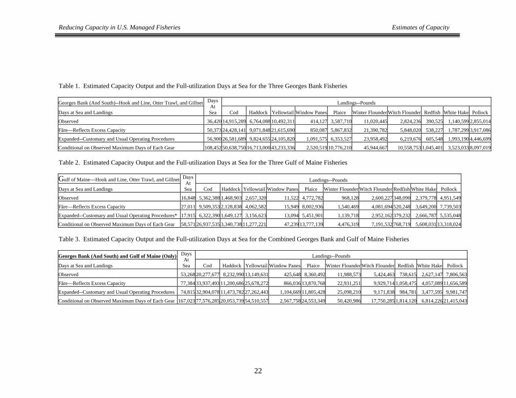
Because of the large number of estimates, we present only summary estimates for Georges Bank, Gulf of Maine, and the two areas combined (Tables 1-3). It is apparent that the fleet could land considerably more than they have been landing. For example, the fleet could land up to 50.6 million pounds of cod from the Georges Bank resource area and up to 26.9 million pounds from the Gulf of Maine resource area. The fact that the vessels could land considerably more than they have, however, does not equate to having overcapacity. That is, the fleet could have excess capacity in the sense that they have the capability to harvest more than they actually did, even with depressed resource conditions. The critical issue is whether or not the fleet could harvest in excess of MSY for each species if resource levels were restored to their desired target levels. With respect to overcapacity, the fleet really only has overcapacity relative to Plaice, winter flounder, and witch flounder (Table 4). That is, if resource levels were restored to levels consistent with supporting the long-term potential yield, the fleet would have insufficient capability to over-harvest cod, haddock, yellowtail flounder, window pane, redfish, white hake, and Pollock. The fleet, however, would have the capability to harvest in excess of the MSY levels for Plaice, winter flounder, and witch flounder. As a consequence, overcapacity is determined relative to the most binding level of overcapacity. The most binding level of overcapacity is determined according to the largest number of vessels that must be removed to ensure that harvest levels do not exceed the MSY or long-term potential yields of any one species. In this case, the most binding or severe level of overcapacity is determined relative to witch flounder. That is, the largest number of vessels need to be reduced to ensure that the fleet cannot harvest in excess of the long-term potential yield of witch flounder. To ensure that the fleet cannot harvest in excess of the long-term potential yield of witch flounder, 588 vessels need to be removed from the fleet. Based on the assumption that the cost of each vessel equals approximately one year’s gross stock or total revenue, it is estimated that it would cost approximately $259.6 million to buyback the 588 vessels (Table 5). A remaining concern relating to capacity in the New England groundfish fishery was latent permits. There are 725 latent permits; that is, individuals hold permits to land groundfish, but may not have a vessel or may not fish regularly for groundfish. The potential output for these vessels was not estimated. It was possible, however, to estimate the potential buyback cost for these vessels. Using information on a previous buyback program in New England, which involved the purchase of permits, it was possible to regress the permit purchase price against the vessel characteristics, and to subsequently use these estimates to calculate the potential cost of purchasing all 725 latent permits. Based on the estimated relationship between permit purchase price, vessel tonnage, engine size, and vessel length, it was estimated that it would cost approximately $190.0 million to purchase the latent permits.
Reducing Capacity in U.S. Managed Fisheries Estimates of Capacity
22
Table 1. Estimated Capacity Output and the Full-utilization Days at Sea for the Three Georges Bank Fisheries Georges Bank (And South)--Hook and Line, Otter Trawl, and Gillnet Landings--Pounds
Days at Sea and Landings
Days At Sea Cod Haddock Yellowtail Window Panes Plaice Winter Flounder Witch Flounder Redfish White Hake Pollock
Observed 36,420 14,915,289 6,764,088 10,492,311 414,127 3,587,710 11,020,445 2,824,236 390,525 1,140,599 2,855,014
F@re—Reflects Excess Capacity 50,373 24,428,141 9,071,848 21,615,690 850,087 5,867,832 21,390,782 5,848,020 538,227 1,787,299 3,917,086
Expanded--Customary and Usual Operating Procedures 56,900 26,581,689 9,824,655 24,105,820 1,091,575 6,353,527 23,958,492 6,219,676 605,548 1,993,190 4,446,699
Conditional on Observed Maximum Days of Each Gear 108,452 50,638,750 16,713,000 43,233,336 2,520,519 10,776,210 45,944,667 10,558,753 1,045,401 3,523,033 8,097,019 Table 2. Estimated Capacity Output and the Full-utilization Days at Sea for the Three Gulf of Maine Fisheries Gulf of Maine—Hook and Line, Otter Trawl, and Gillnet Landings--Pounds
Days at Sea and Landings
DaysAt Sea Cod Haddock Yellowtail Window Panes Plaice Winter Flounder Witch Flounder Redfish White Hake Pollock
Observed 16,848 5,362,388 1,468,903 2,657,320 11,522 4,772,782 968,128 2,600,227 348,090 2,379,778 4,951,549
F@re—Reflects Excess Capacity 27,011 9,509,353 2,128,838 4,062,582 15,949 8,002,936 1,540,469 4,081,694 520,248 3,649,200 7,739,503
Expanded--Customary and Usual Operating Procedures* 17,915 6,322,390 1,649,127 3,156,623 13,094 5,451,901 1,139,718 2,952,162 379,232 2,666,787 5,535,048
Conditional on Observed Maximum Days of Each Gear 58,571 26,937,535 3,340,738 11,277,221 47,239 13,777,139 4,476,319 7,191,532 768,719 5,608,031 13,318,024 Table 3. Estimated Capacity Output and the Full-utilization Days at Sea for the Combined Georges Bank and Gulf of Maine Fisheries Georges Bank (And South) and Gulf of Maine (Only) Landings--Pounds
Days at Sea and Landings
Days At Sea Cod Haddock Yellowtail Window Panes Plaice Winter Flounder Witch Flounder Redfish White Hake Pollock
Observed 53,268 20,277,677 8,232,990 13,149,631 425,648 8,360,492 11,988,573 5,424,463 738,615 2,627,147 7,806,563
F@re—Reflects Excess Capacity 77,384 33,937,493 11,200,686 25,678,272 866,036 13,870,768 22,931,251 9,929,714 1,058,475 4,057,089 11,656,589
Expanded--Customary and Usual Operating Procedures 74,815 32,904,078 11,473,782 27,262,443 1,104,669 11,805,428 25,098,210 9,171,838 984,781 3,477,595 9,981,747
Conditional on Observed Maximum Days of Each Gear 167,023 77,576,285 20,053,739 54,510,557 2,567,758 24,553,349 50,420,986 17,750,285 1,814,120 6,814,226 21,415,043
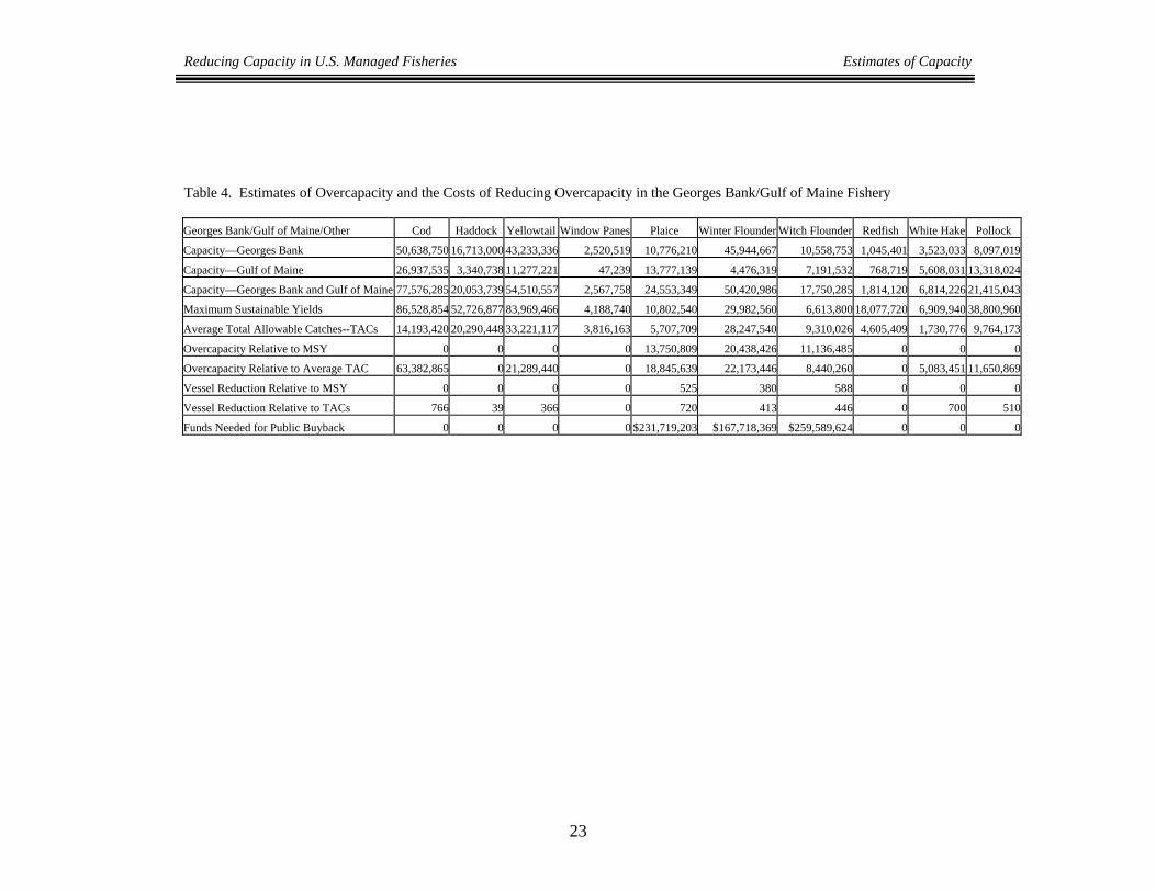
Reducing Capacity in U.S. Managed Fisheries Estimates of Capacity
23
Table 4. Estimates of Overcapacity and the Costs of Reducing Overcapacity in the Georges Bank/Gulf of Maine Fishery Georges Bank/Gulf of Maine/Other Cod Haddock Yellowtail Window Panes Plaice Winter Flounder Witch Flounder Redfish White Hake Pollock
Capacity—Georges Bank 50,638,750 16,713,000 43,233,336 2,520,519 10,776,210 45,944,667 10,558,753 1,045,401 3,523,033 8,097,019
Capacity—Gulf of Maine 26,937,535 3,340,738 11,277,221 47,239 13,777,139 4,476,319 7,191,532 768,719 5,608,031 13,318,024
Capacity—Georges Bank and Gulf of Maine 77,576,285 20,053,739 54,510,557 2,567,758 24,553,349 50,420,986 17,750,285 1,814,120 6,814,226 21,415,043
Maximum Sustainable Yields 86,528,854 52,726,877 83,969,466 4,188,740 10,802,540 29,982,560 6,613,800 18,077,720 6,909,940 38,800,960
Average Total Allowable Catches--TACs 14,193,420 20,290,448 33,221,117 3,816,163 5,707,709 28,247,540 9,310,026 4,605,409 1,730,776 9,764,173
Overcapacity Relative to MSY 0 0 0 0 13,750,809 20,438,426 11,136,485 0 0 0
Overcapacity Relative to Average TAC 63,382,865 0 21,289,440 0 18,845,639 22,173,446 8,440,260 0 5,083,451 11,650,869
Vessel Reduction Relative to MSY 0 0 0 0 525 380 588 0 0 0
Vessel Reduction Relative to TACs 766 39 366 0 720 413 446 0 700 510
Funds Needed for Public Buyback 0 0 0 0 $231,719,203 $167,718,369 $259,589,624 0 0 0
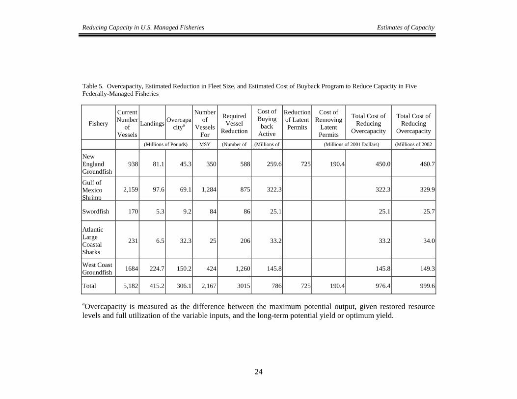
Reducing Capacity in U.S. Managed Fisheries Estimates of Capacity
24
Table 5. Overcapacity, Estimated Reduction in Fleet Size, and Estimated Cost of Buyback Program to Reduce Capacity in Five Federally-Managed Fisheries
Fishery
Current Number
of Vessels
Landings
Overcapa
citya
Number
of Vessels
For
Required Vessel
Reduction
Cost of Buying
back Active V l
Reduction of Latent Permits
Cost of
Removing Latent Permits
Total Cost of
Reducing Overcapacity
Total Cost of
Reducing Overcapacity
(Millions of Pounds) MSY
(OY)(Number of
V l )(Millions of
2001 D ll )
(Millions of 2001 Dollars) (Millions of 2002
D ll ) New England Groundfish
938
81.1
45.3
350
588
259.6
725
190.4
450.0
460.7
Gulf of Mexico Shrimp
2,159
97.6
69.1
1,284
875
322.3
322.3
329.9
Swordfish
170
5.3
9.2
84
86
25.1
25.1
25.7
Atlantic Large Coastal Sharks
231
6.5
32.3
25
206
33.2
33.2
34.0
West Coast Groundfish
1684
224.7
150.2
424
1,260
145.8
145.8
149.3
Total
5,182
415.2
306.1
2,167
3015
786
725
190.4
976.4
999.6
aOvercapacity is measured as the difference between the maximum potential output, given restored resource levels and full utilization of the variable inputs, and the long-term potential yield or optimum yield.
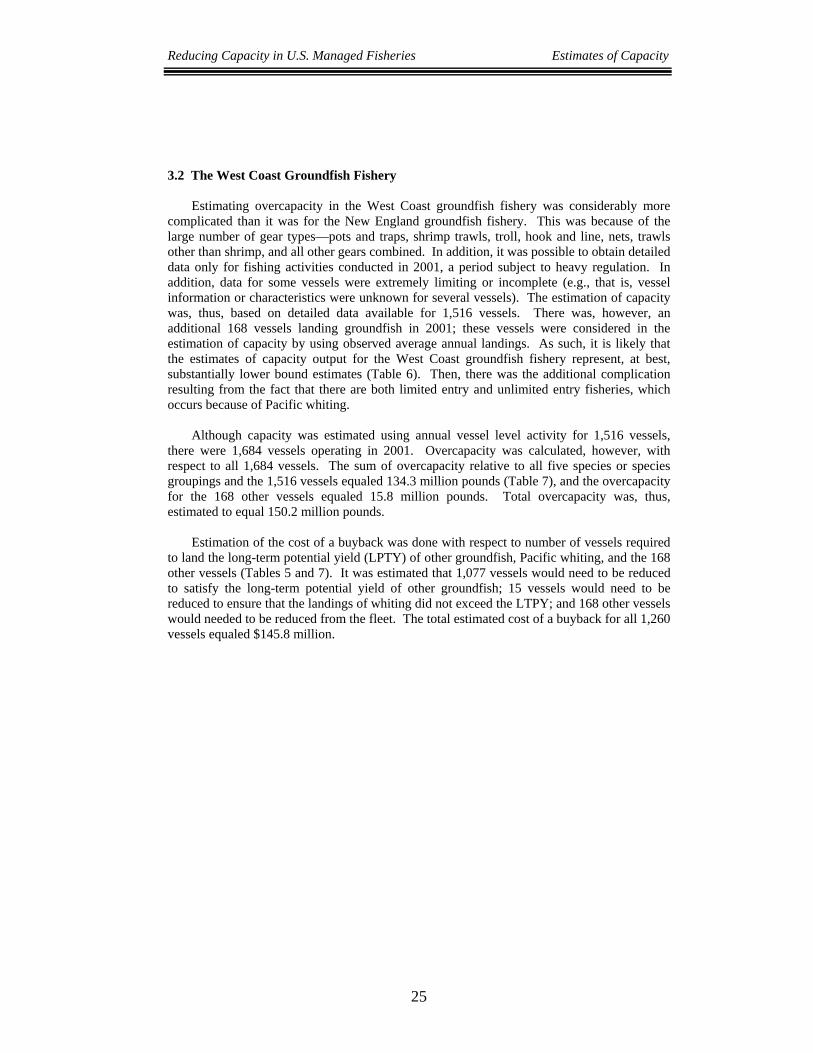
Reducing Capacity in U.S. Managed Fisheries Estimates of Capacity
25
3.2 The West Coast Groundfish Fishery Estimating overcapacity in the West Coast groundfish fishery was considerably more complicated than it was for the New England groundfish fishery. This was because of the large number of gear types—pots and traps, shrimp trawls, troll, hook and line, nets, trawls other than shrimp, and all other gears combined. In addition, it was possible to obtain detailed data only for fishing activities conducted in 2001, a period subject to heavy regulation. In addition, data for some vessels were extremely limiting or incomplete (e.g., that is, vessel information or characteristics were unknown for several vessels). The estimation of capacity was, thus, based on detailed data available for 1,516 vessels. There was, however, an additional 168 vessels landing groundfish in 2001; these vessels were considered in the estimation of capacity by using observed average annual landings. As such, it is likely that the estimates of capacity output for the West Coast groundfish fishery represent, at best, substantially lower bound estimates (Table 6). Then, there was the additional complication resulting from the fact that there are both limited entry and unlimited entry fisheries, which occurs because of Pacific whiting. Although capacity was estimated using annual vessel level activity for 1,516 vessels, there were 1,684 vessels operating in 2001. Overcapacity was calculated, however, with respect to all 1,684 vessels. The sum of overcapacity relative to all five species or species groupings and the 1,516 vessels equaled 134.3 million pounds (Table 7), and the overcapacity for the 168 other vessels equaled 15.8 million pounds. Total overcapacity was, thus, estimated to equal 150.2 million pounds.
Estimation of the cost of a buyback was done with respect to number of vessels required to land the long-term potential yield (LPTY) of other groundfish, Pacific whiting, and the 168 other vessels (Tables 5 and 7). It was estimated that 1,077 vessels would need to be reduced to satisfy the long-term potential yield of other groundfish; 15 vessels would need to be reduced to ensure that the landings of whiting did not exceed the LTPY; and 168 other vessels would needed to be reduced from the fleet. The total estimated cost of a buyback for all 1,260 vessels equaled $145.8 million.
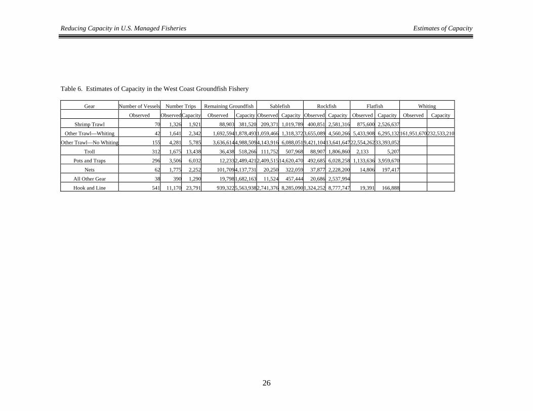
Reducing Capacity in U.S. Managed Fisheries Estimates of Capacity
26
Table 6. Estimates of Capacity in the West Coast Groundfish Fishery
Gear Number of Vessels Number Trips Remaining Groundfish Sablefish Rockfish Flatfish Whiting
Observed ObservedCapacity Observed Capacity Observed Capacity Observed Capacity Observed Capacity Observed Capacity
Shrimp Trawl 70 1,326 1,921 88,903 381,520 209,371 1,019,789 400,851 2,581,316 875,600 2,526,637
Other Trawl—Whiting 42 1,641 2,342 1,692,5941,878,4931,059,466 1,318,3723,655,089 4,560,266 5,433,908 6,295,132161,951,670232,533,210
Other Trawl—No Whiting 155 4,281 5,785 3,636,6144,988,5094,143,916 6,088,0519,421,104 13,641,64722,554,26233,393,052
Troll 312 1,675 13,438 36,438 518,266 111,752 507,968 88,907 1,806,860 2,133 5,207
Pots and Traps 296 3,506 6,032 12,2332,489,4212,409,51514,620,470 492,685 6,028,258 1,133,636 3,959,670
Nets 62 1,775 2,252 101,7094,137,731 20,250 322,059 37,877 2,228,200 14,806 197,417
All Other Gear 38 390 1,290 19,7981,682,163 11,524 457,444 20,686 2,537,994
Hook and Line 541 11,170 23,791 939,3225,563,9382,741,376 8,285,0901,324,252 8,777,747 19,391 166,888
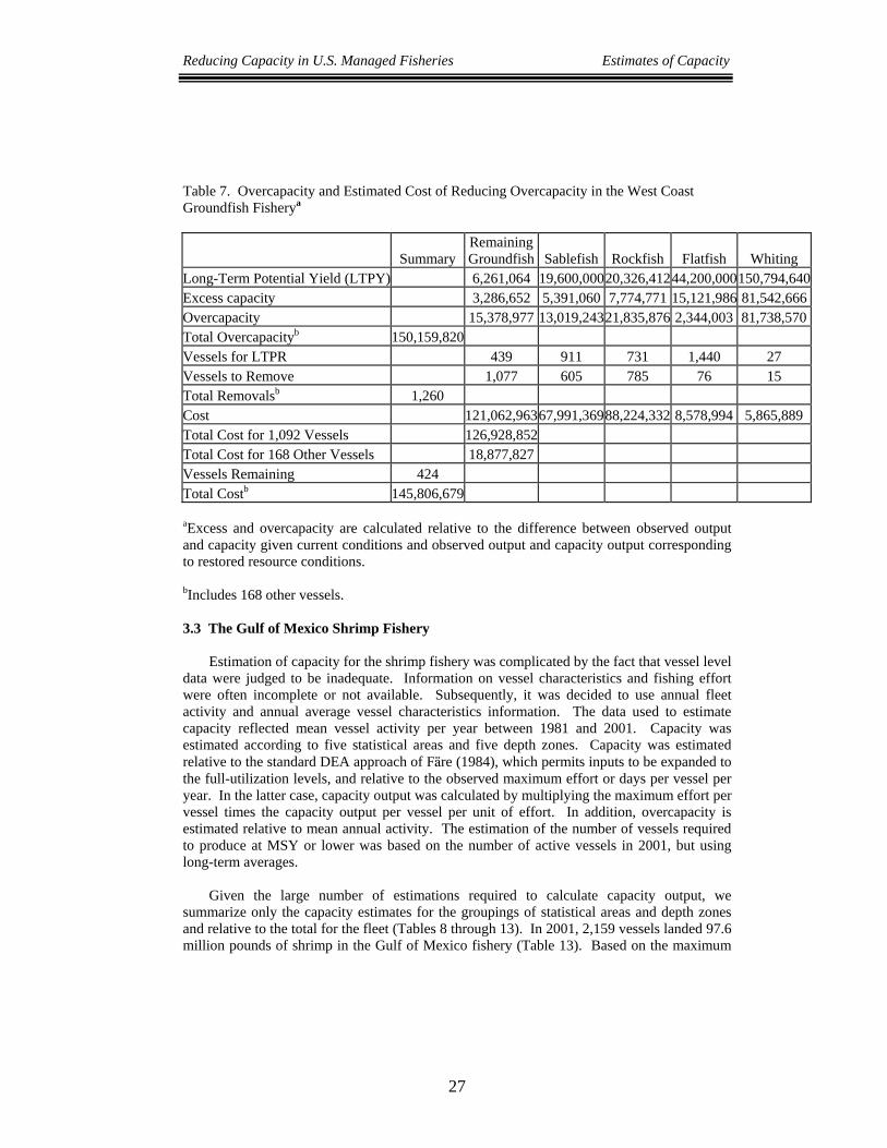
Reducing Capacity in U.S. Managed Fisheries Estimates of Capacity
27
Table 7. Overcapacity and Estimated Cost of Reducing Overcapacity in the West Coast Groundfish Fisherya
Summary RemainingGroundfish Sablefish Rockfish Flatfish Whiting
Long-Term Potential Yield (LTPY) 6,261,064 19,600,00020,326,412 44,200,000150,794,640Excess capacity 3,286,652 5,391,060 7,774,771 15,121,986 81,542,666Overcapacity 15,378,977 13,019,24321,835,876 2,344,003 81,738,570Total Overcapacityb 150,159,820 Vessels for LTPR 439 911 731 1,440 27 Vessels to Remove 1,077 605 785 76 15 Total Removalsb 1,260 Cost 121,062,96367,991,36988,224,332 8,578,994 5,865,889 Total Cost for 1,092 Vessels 126,928,852 Total Cost for 168 Other Vessels 18,877,827 Vessels Remaining 424 Total Costb 145,806,679 aExcess and overcapacity are calculated relative to the difference between observed output and capacity given current conditions and observed output and capacity output corresponding to restored resource conditions.
bIncludes 168 other vessels. 3.3 The Gulf of Mexico Shrimp Fishery
Estimation of capacity for the shrimp fishery was complicated by the fact that vessel level data were judged to be inadequate. Information on vessel characteristics and fishing effort were often incomplete or not available. Subsequently, it was decided to use annual fleet activity and annual average vessel characteristics information. The data used to estimate capacity reflected mean vessel activity per year between 1981 and 2001. Capacity was estimated according to five statistical areas and five depth zones. Capacity was estimated relative to the standard DEA approach of F@re (1984), which permits inputs to be expanded to the full-utilization levels, and relative to the observed maximum effort or days per vessel per year. In the latter case, capacity output was calculated by multiplying the maximum effort per vessel times the capacity output per vessel per unit of effort. In addition, overcapacity is estimated relative to mean annual activity. The estimation of the number of vessels required to produce at MSY or lower was based on the number of active vessels in 2001, but using long-term averages.
Given the large number of estimations required to calculate capacity output, we
summarize only the capacity estimates for the groupings of statistical areas and depth zones and relative to the total for the fleet (Tables 8 through 13). In 2001, 2,159 vessels landed 97.6 million pounds of shrimp in the Gulf of Mexico fishery (Table 13). Based on the maximum

Reducing Capacity in U.S. Managed Fisheries Estimates of Capacity
28
average annual number of days per vessel in each fishing area and depth zone (the average of total effort for a fleet divided by number of vessels; e.g., Table 14), it is estimated that 1,284 vessels could harvest the MSY level of shrimp. Therefore, 875 vessels could be removed from the 2001 fleet. The estimated cost of reducing the fleet in 2001 constant dollars is $322.3 million (Tables 5 and 13). Given that capacity was estimated using fleet wide averages, it is likely that capacity output is underestimated for the Gulf of Mexico shrimp fishery. The use of fleet wide average information limits the number of observations, which in turn, limits the projection of the frontier technology. In essence, there is a tendency to underestimate capacity output when estimation is based on a limited number of observations and the data reflect mean values. Table 8. Estimates of Capacity Output for Area 5 and Five Corresponding Depth Zones, Gulf of Mexico Shrimp Fishery
Average Annual Activity
Area
Depth Zone
Level Of
Activity
Effort
Vessels
Pounds
Value
Over Capacity
(lbs)
Vessels Required
For MSY
Levela
PotentialRemovala
5 5 Observed 324 39 115,486 782,899 F@re—Excess Capacity 362 39 154,105 1,069,841 38,619 18 3 Max Days 528 39 225,906 1,592,815 110,421 15 65 4 Observed 4,107 315 1,577,047 10,189,773 F@re—Excess Capacity 4,293 315 1,853,495 12,071,409 276,448 180 34 Max Days 8,807 315 3,933,832 25,836,914 2,356,785 76 1385 3 Observed 15,662 718 7,248,447 41,670,398 F@re—Excess Capacity 16,750 718 8,067,106 46,406,283 818,659 407 90 Max Days 21,554 718 10,502,488 61,653,818 3,254,041 279 2185 2 Observed 28,723 1,280 16,653,080 75,731,391 F@re—Excess Capacity 27,860 1,280 19,390,292 88,642,495 2,737,212 903 436 Max Days 43,518 1,280 30,978,110 142,864,559 14,325,030 494 8455 1 Observed 15,800 1,012 6,780,903 32,321,385 F@re—Excess Capacity 16,459 1,012 7,594,850 35,938,708 813,947 673 -21 Max Days 28,345 1,012 13,288,632 64,061,800 6,507,729 448 204 aAlthough the estimates of capacity output are based on average annual activity, the estimated reduction in number of vessels to eliminate overcapacity is determined relative to the existing number of vessels in 2001. That is, using average annual activity, the number of vessels, on average, required to produce the MSY level is initially calculated, and then, that number is subtracted from the actual number of vessels operating in 2001. The MSY level is assumed to equal the average annual landings for each area and depth zone.
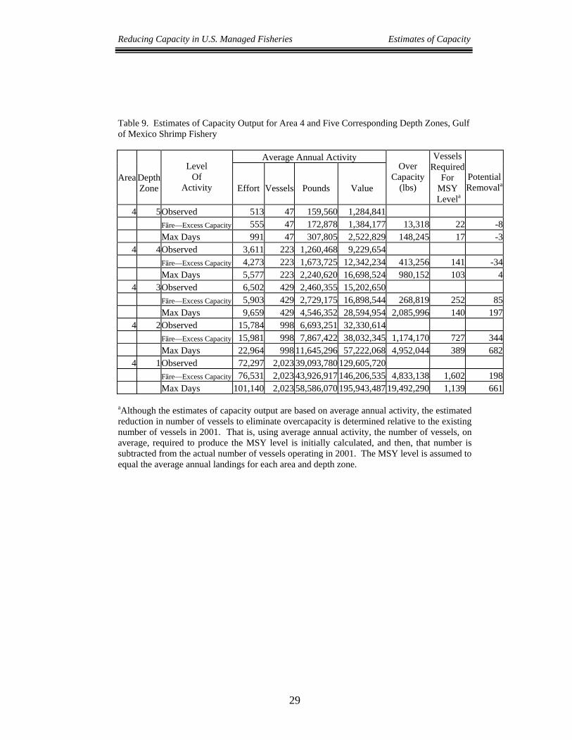
Reducing Capacity in U.S. Managed Fisheries Estimates of Capacity
29
Table 9. Estimates of Capacity Output for Area 4 and Five Corresponding Depth Zones, Gulf of Mexico Shrimp Fishery
Average Annual Activity
Area
Depth Zone
Level Of
Activity
Effort
Vessels
Pounds
Value
Over Capacity
(lbs)
Vessels Required
For MSY
Levela
PotentialRemovala
4 5Observed 513 47 159,560 1,284,841
F@re—Excess Capacity 555 47 172,878 1,384,177 13,318 22 -8 Max Days 991 47 307,805 2,522,829 148,245 17 -3
4 4Observed 3,611 223 1,260,468 9,229,654 F@re—Excess Capacity 4,273 223 1,673,725 12,342,234 413,256 141 -34 Max Days 5,577 223 2,240,620 16,698,524 980,152 103 4
4 3Observed 6,502 429 2,460,355 15,202,650 F@re—Excess Capacity 5,903 429 2,729,175 16,898,544 268,819 252 85 Max Days 9,659 429 4,546,352 28,594,954 2,085,996 140 197
4 2Observed 15,784 998 6,693,251 32,330,614 F@re—Excess Capacity 15,981 998 7,867,422 38,032,345 1,174,170 727 344 Max Days 22,964 998 11,645,296 57,222,068 4,952,044 389 682
4 1Observed 72,297 2,023 39,093,780 129,605,720 F@re—Excess Capacity 76,531 2,023 43,926,917 146,206,535 4,833,138 1,602 198 Max Days 101,140 2,023 58,586,070 195,943,487 19,492,290 1,139 661 aAlthough the estimates of capacity output are based on average annual activity, the estimated reduction in number of vessels to eliminate overcapacity is determined relative to the existing number of vessels in 2001. That is, using average annual activity, the number of vessels, on average, required to produce the MSY level is initially calculated, and then, that number is subtracted from the actual number of vessels operating in 2001. The MSY level is assumed to equal the average annual landings for each area and depth zone.
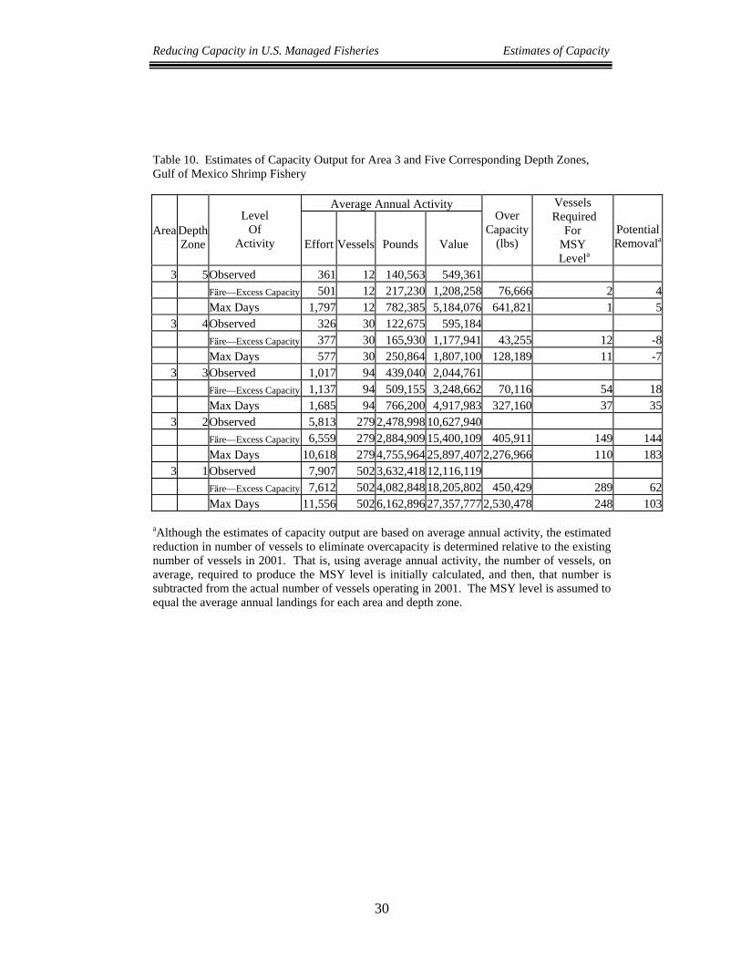
Reducing Capacity in U.S. Managed Fisheries Estimates of Capacity
30
Table 10. Estimates of Capacity Output for Area 3 and Five Corresponding Depth Zones, Gulf of Mexico Shrimp Fishery
Average Annual Activity
Area
Depth Zone
Level Of
Activity
Effort
Vessels
Pounds
Value
Over Capacity
(lbs)
Vessels Required
For MSY
Levela
PotentialRemovala
3 5Observed 361 12 140,563 549,361
F@re—Excess Capacity 501 12 217,230 1,208,258 76,666 2 4 Max Days 1,797 12 782,385 5,184,076 641,821 1 5
3 4Observed 326 30 122,675 595,184 F@re—Excess Capacity 377 30 165,930 1,177,941 43,255 12 -8 Max Days 577 30 250,864 1,807,100 128,189 11 -7
3 3Observed 1,017 94 439,040 2,044,761 F@re—Excess Capacity 1,137 94 509,155 3,248,662 70,116 54 18 Max Days 1,685 94 766,200 4,917,983 327,160 37 35
3 2Observed 5,813 279 2,478,998 10,627,940 F@re—Excess Capacity 6,559 279 2,884,909 15,400,109 405,911 149 144 Max Days 10,618 279 4,755,964 25,897,407 2,276,966 110 183
3 1Observed 7,907 502 3,632,418 12,116,119 F@re—Excess Capacity 7,612 502 4,082,848 18,205,802 450,429 289 62 Max Days 11,556 502 6,162,896 27,357,777 2,530,478 248 103 aAlthough the estimates of capacity output are based on average annual activity, the estimated reduction in number of vessels to eliminate overcapacity is determined relative to the existing number of vessels in 2001. That is, using average annual activity, the number of vessels, on average, required to produce the MSY level is initially calculated, and then, that number is subtracted from the actual number of vessels operating in 2001. The MSY level is assumed to equal the average annual landings for each area and depth zone.
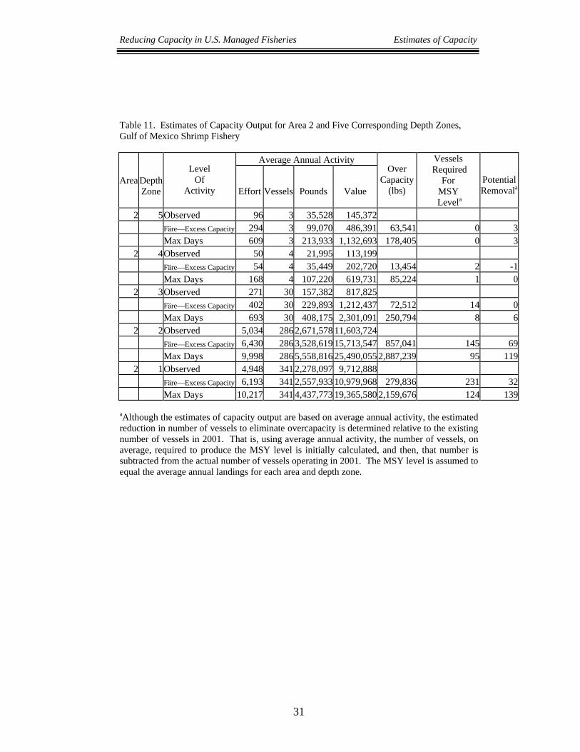
Reducing Capacity in U.S. Managed Fisheries Estimates of Capacity
31
Table 11. Estimates of Capacity Output for Area 2 and Five Corresponding Depth Zones, Gulf of Mexico Shrimp Fishery
Average Annual Activity
Area
Depth Zone
Level Of
Activity
Effort
Vessels
Pounds
Value
Over Capacity
(lbs)
Vessels Required
For MSY
Levela
PotentialRemovala
2 5Observed 96 3 35,528 145,372
F@re—Excess Capacity 294 3 99,070 486,391 63,541 0 3 Max Days 609 3 213,933 1,132,693 178,405 0 3
2 4Observed 50 4 21,995 113,199 F@re—Excess Capacity 54 4 35,449 202,720 13,454 2 -1 Max Days 168 4 107,220 619,731 85,224 1 0
2 3Observed 271 30 157,382 817,825 F@re—Excess Capacity 402 30 229,893 1,212,437 72,512 14 0 Max Days 693 30 408,175 2,301,091 250,794 8 6
2 2Observed 5,034 286 2,671,578 11,603,724 F@re—Excess Capacity 6,430 286 3,528,619 15,713,547 857,041 145 69 Max Days 9,998 286 5,558,816 25,490,055 2,887,239 95 119
2 1Observed 4,948 341 2,278,097 9,712,888 F@re—Excess Capacity 6,193 341 2,557,933 10,979,968 279,836 231 32 Max Days 10,217 341 4,437,773 19,365,580 2,159,676 124 139 aAlthough the estimates of capacity output are based on average annual activity, the estimated reduction in number of vessels to eliminate overcapacity is determined relative to the existing number of vessels in 2001. That is, using average annual activity, the number of vessels, on average, required to produce the MSY level is initially calculated, and then, that number is subtracted from the actual number of vessels operating in 2001. The MSY level is assumed to equal the average annual landings for each area and depth zone.
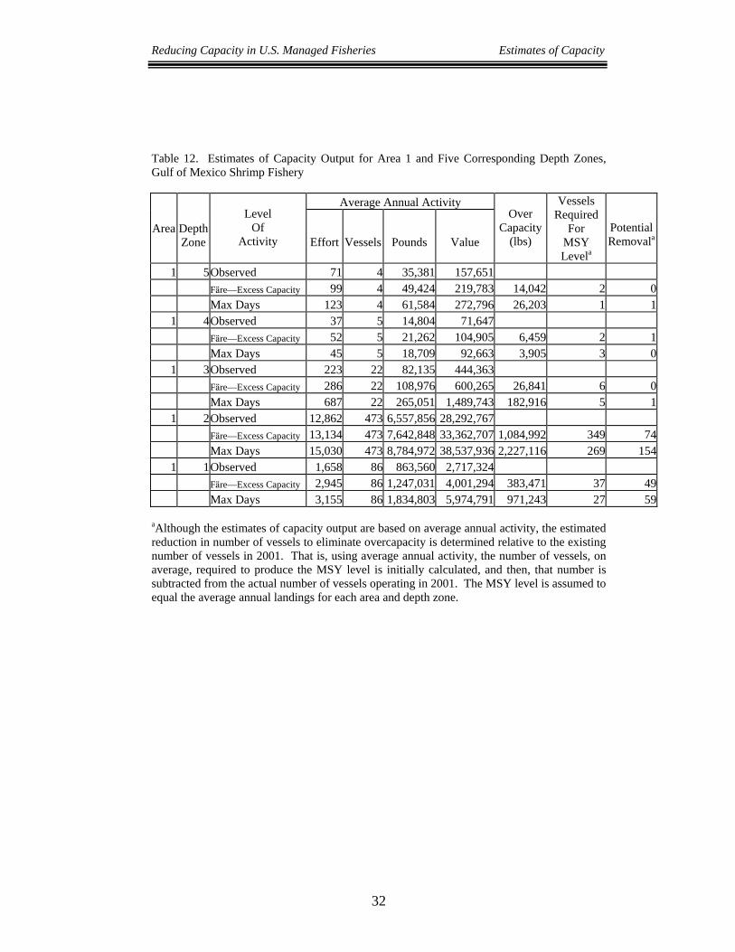
Reducing Capacity in U.S. Managed Fisheries Estimates of Capacity
32
Table 12. Estimates of Capacity Output for Area 1 and Five Corresponding Depth Zones, Gulf of Mexico Shrimp Fishery
Average Annual Activity
Area
Depth Zone
Level Of
Activity
Effort
Vessels
Pounds
Value
Over Capacity
(lbs)
Vessels Required
For MSY Levela
PotentialRemovala
1 5Observed 71 4 35,381 157,651
F@re—Excess Capacity 99 4 49,424 219,783 14,042 2 0 Max Days 123 4 61,584 272,796 26,203 1 1
1 4Observed 37 5 14,804 71,647 F@re—Excess Capacity 52 5 21,262 104,905 6,459 2 1 Max Days 45 5 18,709 92,663 3,905 3 0
1 3Observed 223 22 82,135 444,363 F@re—Excess Capacity 286 22 108,976 600,265 26,841 6 0 Max Days 687 22 265,051 1,489,743 182,916 5 1
1 2Observed 12,862 473 6,557,856 28,292,767 F@re—Excess Capacity 13,134 473 7,642,848 33,362,707 1,084,992 349 74 Max Days 15,030 473 8,784,972 38,537,936 2,227,116 269 154
1 1Observed 1,658 86 863,560 2,717,324 F@re—Excess Capacity 2,945 86 1,247,031 4,001,294 383,471 37 49 Max Days 3,155 86 1,834,803 5,974,791 971,243 27 59 aAlthough the estimates of capacity output are based on average annual activity, the estimated reduction in number of vessels to eliminate overcapacity is determined relative to the existing number of vessels in 2001. That is, using average annual activity, the number of vessels, on average, required to produce the MSY level is initially calculated, and then, that number is subtracted from the actual number of vessels operating in 2001. The MSY level is assumed to equal the average annual landings for each area and depth zone.
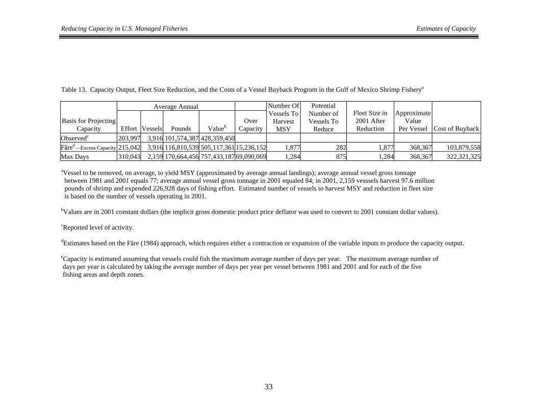
Reducing Capacity in U.S. Managed Fisheries Estimates of Capacity
33
Table 13. Capacity Output, Fleet Size Reduction, and the Costs of a Vessel Buyback Program in the Gulf of Mexico Shrimp Fisherya
Average Annual
Basis for Projecting Capacity Effort Vessels Pounds Valueb
Over Capacity
Number OfVessels To
Harvest MSY
Potential Number of Vessels To
Reduce
Fleet Size in 2001 After Reduction
ApproximateValue
Per Vessel Cost of BuybackObservedc 203,997 3,916 101,574,387 428,359,450 F@red—Excess Capacity 215,042 3,916 116,810,539 505,117,361 15,236,152 1,877 282 1,877 368,367 103,879,558Max Days 310,043 2,159 170,664,456 757,433,187 69,090,069 1,284 875 1,284 368,367 322,321,325 aVessel to be removed, on average, to yield MSY (approximated by average annual landings); average annual vessel gross tonnage between 1981 and 2001 equals 77; average annual vessel gross tonnage in 2001 equaled 84; in 2001, 2,159 vesssels harvest 97.6 million pounds of shrimp and expended 226,928 days of fishing effort. Estimated number of vessels to harvest MSY and reduction in fleet size is based on the number of vessels operating in 2001. bValues are in 2001 constant dollars (the implicit gross domestic product price deflator was used to convert to 2001 constant dollar values). cReported level of activity. dEstimates based on the F@re (1984) approach, which requires either a contraction or expansion of the variable inputs to produce the capacity output. eCapacity is estimated assuming that vessels could fish the maximum average number of days per year. The maximum average number of days per year is calculated by taking the average number of days per year per vessel between 1981 and 2001 and for each of the five fishing areas and depth zones.
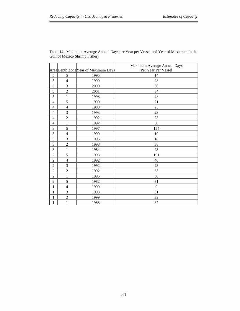
Reducing Capacity in U.S. Managed Fisheries Estimates of Capacity
34
Table 14. Maximum Average Annual Days per Year per Vessel and Year of Maximum In the Gulf of Mexico Shrimp Fishery
Area Depth ZoneYear of Maximum DaysMaximum Average Annual Days
Per Year Per Vessel 5 5 1995 14 5 4 1990 28 5 3 2000 30 5 2 2001 34 5 1 1998 28 4 5 1990 21 4 4 1988 25 4 3 1993 23 4 2 1992 23 4 1 1992 50 3 5 1997 154 3 4 1990 19 3 3 1995 18 3 2 1998 38 3 1 1984 23 2 5 1993 191 2 4 1992 40 2 3 1992 23 2 2 1992 35 2 1 1996 30 2 5 1982 31 1 4 1990 9 1 3 1993 31 1 2 1999 32 1 1 1988 37
Reducing Capacity in U.S. Managed Fisheries Estimates of Capacity
35
3.4 The Atlantic Swordfish Fishery
Capacity output for the swordfish fishery was estimated using data on area fished, total number of vessels operating in an area in a year, number of hooks, number of miles of longline, and number of days. This information was the most complete information available on the fishery. Capacity output was calculated relative to the TACs in 2000 and the long-term potential yields, which was set equal to the sum of U.S. shares of the maximum sustainable yields for the north and south Atlantic areas. Capacity was also estimated using the number of days corresponding to full-variable input utilization and the actual reported total days per year. The analysis suggested that the fleet could reduce the number of days per year and still harvest the same level of swordfish. The cost of the buyback program was calculated assuming the fleet would fish the reported number of days in each year.
The analysis of capacity revealed that the fleet had substantial overcapacity in 2000, the
year for which the data were the most current. The fleet had the capability to harvest 9.2 million pounds more than the long-term potential yield of nearly 9.0 million pounds (Tables 15 and 16). The number of vessels necessary to harvest the long-term potential yield, with no change in the number of days at sea relative to the number of days reported in 2000, was estimated to equal 84. In 2000, the actual number of vessels landing swordfish was 170. The analysis, thus, suggest that the number of vessels could be reduced by 86 relative to the number of vessels operating in 2000. Using average annual gross stock per vessel, again this pertains to the gross stock from all fisheries for a given vessel, it was estimated that the dollars necessary to purchase the 86 vessels equaled $25.1 million (Tables 5 and 16).
One result that stands out relative to the analyses of the other fisheries is the projection
that days at sea should be substantially reduced to harvest the capacity output. At the annual mean level, the fleet is expending 40% more effort, in terms of days at sea, than it needs to expend. This is clearly indicative of rather severe technical inefficiency. Alternatively, capacity output could be realized mostly through gains in technical efficiency. The reasons for the high level of inefficiency, however, are not known. They may be related to resource conditions, changes in prices, weather patterns, and management and regulation of the fishery.
The estimates of capacity output for the swordfish fishery, however, are likely to be
extremely low or downwards biased. This is because of declining resource levels and intense regulation, which have limited the landings of swordfish. Alternatively, none of the years included in the analysis were years during which resource levels were at their MSY levels. In addition, the use of fleet-wide information tends to result in underestimating capacity output. This is because there are fewer data points to construct the frontier technology, which, in turn, tends to force the frontier to be equivalent to the observed production activities.

Reducing Capacity in U.S. Managed Fisheries Estimates of Capacity
36
Table 15. Capacity Output for the U.S. North and South Atlantic Swordfish Fisheries
Year
Number of
Vessels
Swordfish kept
(number)
Weight (lbs)
Number of hooks
Number of
Mainline Miles
Number Of
Days
Days Required
to Harvest Capacity Output
Capacity Given Fleet
Reduces Days (lbs)
Capacity Given
Fleet FishesObserved Number Of Days per Year
(lbs)
1987 260 111,290 7,987,283 4,632,653 304,196 11,863 7,611 15,447,956 24,078,1271988 299 146,623 10,523,133 5,096,433 324,808 12,615 8,403 17,405,649 26,128,9791990 316 129,052 9,262,062 5,680,414 365,344 14,170 9,561 19,978,252 29,610,3201991 237 85,528 6,138,345 5,286,425 299,605 11,730 8,265 17,477,999 24,806,0371992 238 62,286 4,470,266 5,268,494 265,313 10,257 7,717 16,068,056 21,356,1151993 245 62,922 4,515,912 5,517,101 263,965 10,345 7,714 16,309,048 21,872,1691994 244 63,738 4,574,476 5,451,459 269,662 10,035 7,939 16,998,160 21,486,1671995 255 72,680 5,216,244 6,778,583 324,768 11,153 8,468 18,154,814 23,911,7511996 235 72,980 5,237,775 6,688,529 288,654 11,168 8,112 17,943,367 24,704,4371997 230 68,263 4,899,236 6,071,732 264,222 10,006 7,287 16,061,302 22,054,1091998 191 68,345 4,905,121 5,469,457 231,892 8,686 6,580 14,561,438 19,221,0771999 174 64,112 4,601,318 5,003,082 200,748 8,024 5,695 12,711,816 17,910,9152000 170 60,913 4,371,726 5,308,229 224,157 8,279 5,643 12,397,302 18,189,099
Mean 238 82,210 5,900,223 5,557,892 279,026 10,641 7,615 16,270,397 22,717,639 Table 16. Estimated Cost of Reducing 86 Swordfish Vesselsa Long-term Potential Yield (LPTY) lbs live 8,996,267 2000 Excess Capacity—lbs live 12,397,302 2000 Overcapacity--lbs live 18,189,099 Number of Vessel in 2000 170 Vessels for LTPY 84 Vessel Reduction Given Number of Vessels in 2000 86 Cost of Purchasing 86 Vessels 25,116,813 aEstimates are based on assumption that fleet would fish the number of days reported for 2000, which is the year for which the data are most recent. In 2000, the fleet had the potential to land 18.2 million pounds of swordfish, and the long-term potential yield is nearly 9.0 million pounds. The fleet had overcapacity of 9.2 million pounds in 2000.

Reducing Capacity in U.S. Managed Fisheries Estimates of Capacity
37
3.5 The Large Coastal Pelagic Shark Fishery
The large coastal pelagic shark fishery involves more than 25 different types of sharks. There are three primary gear types—longline, gillnet, and pelagic gear. The longline and gillnet fisheries primarily target black tip and sand sharks, while the pelagic gear primarily targets up to 13 different kinds of sharks. For the pelagic gear type, however, many of the different kinds of sharks are not frequently captured or are captured in very low quantities. Capacity output was subsequently estimating relative to all three types of gear and a composite or aggregate output, which equaled the sum of all shark landings.
The assumed fixed and variable inputs were designated by three gear types. First, in the
pelagic gear fishery, vessel length and vessel hold size were assumed fixed, while days at sea were assumed to be variable. In the gillnet fishery, the inputs assumed to be fixed factors were vessel length, fishing effort, length of net, and crew size, while days at sea were assumed to be variable. Finally, in the longline fishery, the inputs assumed to be fixed factors were vessel length, vessel hold size, fishing effort, length of the longline, and crew size, while days at sea were assumed to be variable. Subsequently, trip level information was aggregated to annual vessel performance. These data were used to estimate capacity for the large coastal pelagic shark fishery. Estimates of maximum sustainable yield for each species were not available, and thus, MSY was calculated as being equal to the sum of average annual landings of each species of shark between 1990 and 2000. The sum of average annual landings, however, was considerably lower than the sum of quotas imposed on each species or various species of sharks. It was subsequently decided to calculate the capacity output and number of vessels to potentially remove from the fishery using the quota necessary to achieve MSY—3.9 million pounds. In addition, the calculation of capacity output was restricted to the number of days required to produce the capacity output rather than the number of days (8,547 days), which based on observed activity, the fleet might be able to be at sea during a year (16,667 days).
Although the analysis was based on mean annual vessel performance between 1998 and
2000, we present a summary of fleet wide activity only for 2000 (Table 17). This is because estimates of the number of vessels necessary to harvest the quota necessary to support MSY are based on the number of vessels operating in 2000, the most recent year for which data were available. As indicated in Table 16, the longline fleet is the primary fleet in terms of landings of coastal pelagic sharks. In 2000, the longline fleet landed 85% of the total landings of sharks in the coastal shark fishery. The pelagic gear landed slightly less than 5% of total landings. The longline fleet also had the highest observed landings per day at sea; 7,579 pounds. The gillnet fleet had the second highly observed landings per day at sea; 5,459 pounds.
Relative to the number of days required to harvest the capacity output, the longline fleet
would require the largest increase in number of days; a 468% increase. The gillnet fleet would require only a modest increase in number of days to harvest the capacity output; a 28.3% increase; the pelagic fleet, if it operated in an efficient manner, could actually land their potential capacity output with fewer days at sea.
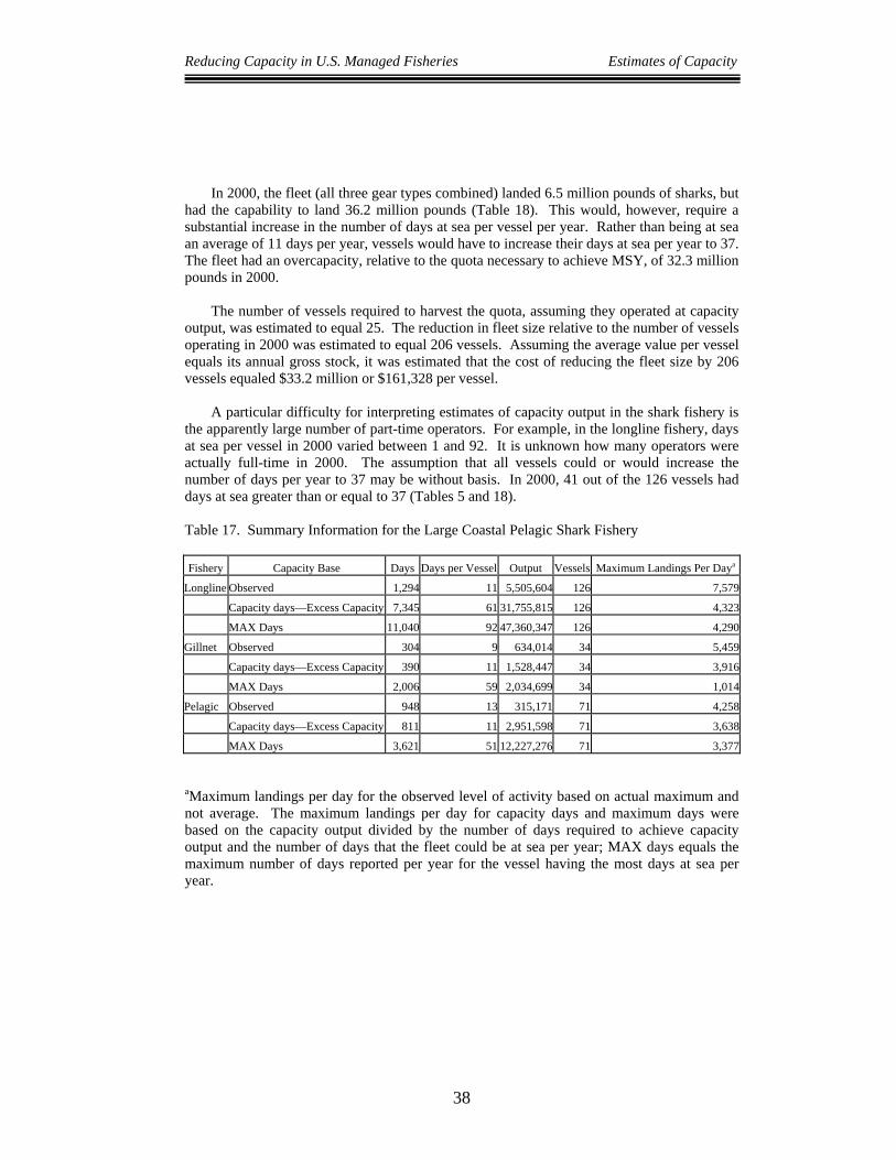
Reducing Capacity in U.S. Managed Fisheries Estimates of Capacity
38
In 2000, the fleet (all three gear types combined) landed 6.5 million pounds of sharks, but had the capability to land 36.2 million pounds (Table 18). This would, however, require a substantial increase in the number of days at sea per vessel per year. Rather than being at sea an average of 11 days per year, vessels would have to increase their days at sea per year to 37. The fleet had an overcapacity, relative to the quota necessary to achieve MSY, of 32.3 million pounds in 2000.
The number of vessels required to harvest the quota, assuming they operated at capacity
output, was estimated to equal 25. The reduction in fleet size relative to the number of vessels operating in 2000 was estimated to equal 206 vessels. Assuming the average value per vessel equals its annual gross stock, it was estimated that the cost of reducing the fleet size by 206 vessels equaled $33.2 million or $161,328 per vessel.
A particular difficulty for interpreting estimates of capacity output in the shark fishery is
the apparently large number of part-time operators. For example, in the longline fishery, days at sea per vessel in 2000 varied between 1 and 92. It is unknown how many operators were actually full-time in 2000. The assumption that all vessels could or would increase the number of days per year to 37 may be without basis. In 2000, 41 out of the 126 vessels had days at sea greater than or equal to 37 (Tables 5 and 18). Table 17. Summary Information for the Large Coastal Pelagic Shark Fishery
Fishery Capacity Base Days Days per Vessel Output Vessels Maximum Landings Per Daya
Longline Observed 1,294 11 5,505,604 126 7,579
Capacity days—Excess Capacity 7,345 61 31,755,815 126 4,323
MAX Days 11,040 92 47,360,347 126 4,290
Gillnet Observed 304 9 634,014 34 5,459
Capacity days—Excess Capacity 390 11 1,528,447 34 3,916
MAX Days 2,006 59 2,034,699 34 1,014
Pelagic Observed 948 13 315,171 71 4,258
Capacity days—Excess Capacity 811 11 2,951,598 71 3,638
MAX Days 3,621 51 12,227,276 71 3,377 aMaximum landings per day for the observed level of activity based on actual maximum and not average. The maximum landings per day for capacity days and maximum days were based on the capacity output divided by the number of days required to achieve capacity output and the number of days that the fleet could be at sea per year; MAX days equals the maximum number of days reported per year for the vessel having the most days at sea per year.
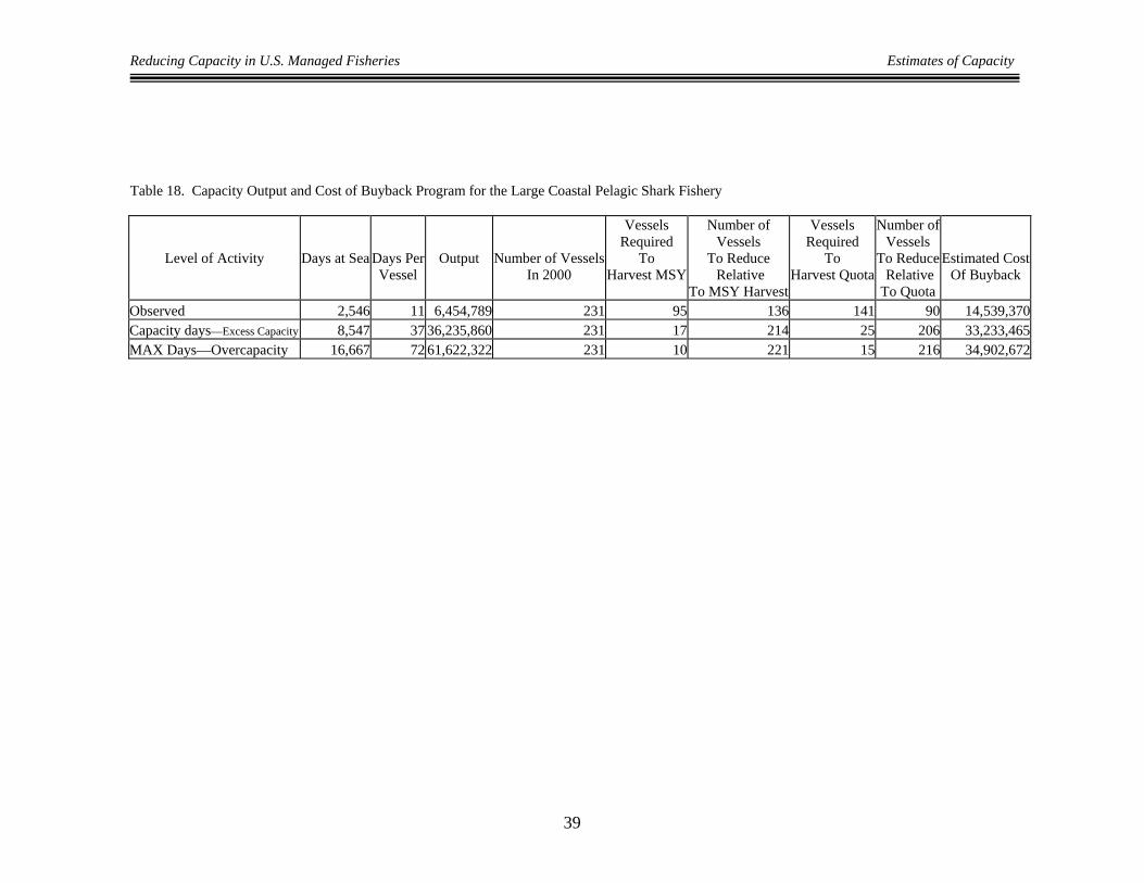
Reducing Capacity in U.S. Managed Fisheries Estimates of Capacity
39
Table 18. Capacity Output and Cost of Buyback Program for the Large Coastal Pelagic Shark Fishery
Level of Activity
Days at Sea
Days PerVessel
Output
Number of VesselsIn 2000
Vessels Required
To Harvest MSY
Number of Vessels
To Reduce Relative
To MSY Harvest
Vessels Required
To Harvest Quota
Number of Vessels
To Reduce RelativeTo Quota
Estimated CostOf Buyback
Observed 2,546 11 6,454,789 231 95 136 141 90 14,539,370Capacity days—Excess Capacity 8,547 37 36,235,860 231 17 214 25 206 33,233,465MAX Days—Overcapacity 16,667 72 61,622,322 231 10 221 15 216 34,902,672
Reducing Capacity in U.S. Managed Fisheries Estimates of Capacity
40
3.6 Overview of Overcapacity and the Cost of a Buyback Program
Relative to the five fisheries examined for this study, it was estimated that fleet size needed to be reduced by 3,015 vessels (Table 5). In contrast, the number of active vessels operating in the fisheries equaled 5,182. It was estimated that 2,167 vessels were required to harvest either the maximum sustainable yields or quotas necessary to achieve MSY. The largest reduction in the number of vessels was for the West Coast groundfish fishery (1,260); the Gulf of Mexico shrimp fishery had the second required largest reduction (875). The New England groundfish fishery required a reduction of 588 vessels, but when latent permits were included, it was estimated that another 725 permits would need to be reduced to prevent overcapacity in the New England groundfish fishery.
The total cost of reducing fleet size to match capacity output to allowable desired target
levels of landings and resources was estimated to be approximately $1.0 billion; this equates to an average buyback cost of $323,847 per vessel. Albeit the estimated buyback cost per vessel may appear high, particularly relative to observed activity in each of the fisheries, it must be considered that the estimated buyback cost is based on retiring the vessel from all commercial fishing. The estimated cost of the buyback program, thus, considers revenues received from other fisheries.
Although the West Coast, groundfish fishery requires the largest vessel reduction to
avoid having overcapacity, the highest direct or vessel buyback program cost is for the Gulf of Mexico shrimp fishery. The New England groundfish fishery has the second highest program cost relative to the direct purchase of vessels; when latent permits are considered, the New England groundfish fishery has the highest buyback cost.
Reducing Capacity in U.S. Managed Fisheries Summary and Conclusions
41
4.0 Summary and Conclusions
The report presented estimates of overcapacity and the potential cost of a government-sponsored buyback program for removing overcapacity in five federally managed fisheries. The five fisheries selected for examination were the New England groundfish fishery, the West Coast groundfish fishery, the Atlantic swordfish fishery, the federal Gulf of Mexico shrimp fishery, and the Atlantic coastal shark fishery. Overcapacity in the two groundfish fisheries was determined relative to the smallest maximum sustainable yield or the species requiring the largest reduction in number of vessels to prevent having overcapacity. Overcapacity for the shrimp and swordfish fisheries were, respectively, determined relative to average annual yield and United States shares of the north and south Atlantic total allowable catches. For the shark fishery, overcapacity was determined relative to the total landings of all sharks combined and an over-all quota necessary to achieve maximum sustainable yield.
Overcapacity was determined to characterize all five fisheries. The most severe case of
overcapacity existed in the West Coast, groundfish fishery; the fleet operating in 2001 had the potential to harvest 150.2 million pounds over the maximum sustainable yield for the fishery. It was also determined that the West Coast, groundfish fishery would require the largest active vessel reduction to prevent overcapacity—1,260 vessels. The New England groundfish fishery, however, may have the potential for having the most severe overcapacity, if latent permits are considered. For example, the analysis suggested that 588 vessels should be reduced from the New England fishery to reduce overcapacity, but 725 latent permits remained that could be activated and used to harvest groundfish. It was also estimated that the total cost of a buyback program to eliminate overcapacity in all five fisheries was approximately $1.0 billion.
The fisheries analyzed for this report constitute approximately 12.5% of the fisheries
under federal management or five out of approximately 40 EEZ fisheries under federal management (http://www.nmfs.noaa.gov/sfa/domes_fish/FMPS.htm). In addition, fishery management plans (FMPs) are under development for nine more fisheries. The extent of overcapacity in many of these other fisheries is not known, but there is significant evidence of excess capacity in several of these fisheries (NMFS Task Force, 2001). Implementing a buyback program, just for the five fisheries examined in this report, would cost nearly $1.0 billion; implementing a buyback program for the other 35 or so fisheries would likely be extremely expensive if the federal government was to fund the buyback.
If the U.S. Congress desires to promote the sustainable use of the nation’s marine
resources and maximization of benefits to society, programs for reducing capacity in many of the EEZ fisheries will have to be developed. Given the expense of buyback programs, it is likely that alternative capacity reduction programs will be necessary. Options for buyback programs include industry sponsorship of buybacks; government financed buybacks, in which the government absorbs either the entire cost or a portion of the cost; and joint industry/government government sponsored buybacks, in which the government offers loans to industry to reduce overcapacity. Alternatively, the use of various management/regulatory strategies could be implemented to rationalize the fleets. One possible management strategy is individual transferable quotas or ITQs. Individual transferable quotas or individual fishing

Reducing Capacity in U.S. Managed Fisheries Summary and Conclusions
42
quotas (IFQs) have worked relatively well in addressing problems in the west coast halibut and sablefish fisheries, the South Atlantic wreckfish fishery, and the surfclam and ocean quahog fishery. The efficient reduction of overcapacity will likely require a combination of capacity reduction actions.
Reducing Capacity in U.S. Managed Fisheries References
43
References Berndt, E. R., and C. J. Morrison. 1981. "Capacity Utilization Measures: Underlying
Economic Theory and an Alternative Approach. " American Economic Review 71:48-52. Berndt, E. R., and M. Fuss. 1989. "Economic Capacity Utilization and Productivity
Measurement for Multiproduct Firms with multiple Quasi-Fixed Inputs." Working paper No. 2932 Cambridge, MA: National Bureau of Economic Research.
Berndt, Ernst R. 1990. A Comment on The Measurement of Capital by Charles R. Hulten, in
Ernst R. Berndt (ed.) Brookings Papers on Economic Activity, 3, pp. 743-756 Charnes, A., W. Cooper, and E. Rhodes. 1978. "Measuring the Efficiency of Decision
Making Units." European Journal of Operational Research 2 (6): 429-444. Coelli T., E. Grifell-Tatje, and S. Perelman. 2001. Capacity utilization and short run profit
efficiency. Manuscript. Presented at the North American Productivity Workshop, June 2000.
Coelli, T. D.S. P. Rao, and G.E. Battese. 1998. An Introduction to Efficiency and
Productivity Analysis. Boston, Kluwer Academic Publishers. F@re, R. 1984. "On the Existence of Plant Capacity." International Economic Review 25
(1):209-213. F@re, R., S. Grosskopf, and C. A. Knox Lovell. 1994. Production Frontiers. New York:
Cambridge University Press. F@re, R., S. Grosskopf, and E. Kokkelenberg. 1989. "Measuring Plant Capacity, Utilization
and Technical Change: A Nonparametric Approach." International Economic Review 30 (3): 656-66.
Färe, R., S. Grosskopf, and J.E. Kirkley. 2000. Multi-output Capacity Measures and Their
Relevance for Productivity. Bulletin of Economic Research (April, 52 (2):101-112. FAO. 2000. Report of the Technical Consultation on the Measurement of Fishing Capacity.
FAO Fisheries, Report No. 615. Rome: Food and Agriculture Organization of the United Nations.
Grafton, R.Q., D. Squires, and J. Kirkley. Turning the tide? Private property rights and the
crisis in fisheries management. Paper #9505E. Department of Economics, University of Ottawa. Contemporary Economic Policy (October 1996), 4:90-99.
Johansen, L. 1968. "Production Functions and the Concept of Capacity." In Recherches
recentes sur la fonction de production. Namur: Centre d'Etudes et de la Recherche Universitaire de Namur.
Reducing Capacity in U.S. Managed Fisheries References
44
Kirkley, J., and D. Squires. 1999. "Capacity and Capacity Utilization in Fishing Industries." Discussion Paper 99-16, University of California, San-Diego.
Kirkley, J., F re, R., Grosskopf, S., McConnell, K., Squires, D., and I. Strand. 2001.
"Assessing Capacity and Capacity Utilization in Fisheries When Data are Limited." North American Journal of Fisheries management 21 (3):482-497.
Kirkley, J.E. and D.E. Squires. 1999b. Measuring capacity and capacity utilization in
fisheries. In: Gréboval, D. (ed) Managing fishing capacity: selected papers on underlying concepts and issues. FAO Fisheries Technical Paper 386, Rome: FAO.
Kirkley, J.E., C.J. Morrison-Paul, and D.E. Squires. 2002a. Capacity and capacity utilization
in common-pool industries. Environmental and Resource Economics 00:1-27. Klein, L.R. 1960, ‘Some Theoretical Issues in the Measurement of Capacity,’ Econometrica
28, pp. 272-286. Klein, L.R. and V. Long. 1973, ‘Capacity Utilization: Concept, Measurement, and Recent
Estimates,’ National Bureau of Economic Research. University of Chicago Press. Morrison, Catherine J. 1985a. Primal and dual capacity utilization: an application to
productivity measurement in the U.S. automobile industry. Journal of Business and Economic Statistics 3:312-324.
Morrison, Catherine J. 1985b. On the economic interpretation and measurement of optimal
capacity utilization with anticipatory expectations. Review of Economic Studies 52:295-310.
National Marine Fisheries Service. 1999. "Federal Fisheries Investment Task Force Report to
Congress." National Marine Fisheries Service, Silver Springs , MD. National Marine Fisheries Service. 2001. "Report of the National Task Force for Defining
and Measuring Fishing Capacity." National Marine Fisheries Service, Silver Springs , MD.
Russell, R.R. 1985. "Measures of Technical Efficiency." Journal of Economic Theory 51:
255-267. Schaefer, M.B. 1954. Some aspects of the dynamics of populations important to the
management of commercial fisheries. Bulletin Inter-American Tropical Tuna Commission 1:27-56.
Segerson, K. and D.E. Squires. 1990. On the measurement of economic capacity utilization
for multi-prodouct industries. Journal of Econometrics 44: 347-361.
Reducing Capacity in U.S. Managed Fisheries References
45
Segerson, K. and D.E. Squires. 1993. Capacity utilization under regulatory constraints. Review of Economics and Statistics 75(1):76-85.
Segerson, K. and D.E. Squires. 1995. Measurement of capacity utilization for revenue-
maximizing firms. Bulletin of Economic Research 47(1):77-84. Snowden, R. 1994. "The Complete Guide to Buying a Business" (Amacom). Squires, D., J. Kirkley, and C.A. Tisdell. 1995. An Individual Transferable Quotas as a
Fisheries Management Tool, Reviews in Fisheries Science, Vol. 3, No. 2, pp. 141-170. Ward, John M., Eric Thunberg, and Pamela Mace (2005). “A Guide to Fish Harvesting
Capacity and Its Relationship to Excess Capacity and Overcapacity.“ Marine Resource Economics, 19:525-529.