Reduced Order Models for Aerodynamic Applications, Loads

REDUCED ORDER MODELS FOR AERODYNAMICAPPLICATIONS, LOADS AND MDO

M. J. Verveld∗ · T. M. Kier∗ · N. W. Karcher† · T. Franz† · M. Abu-Zurayk† · M. Ripepi† · S. Gortz†

Abstract

This work gives an overview of reduced order model (ROM) applications employed within the context of the DLR Digital-Xproject. The ROM methodology has found widespread application in fluid dynamics. In its direct application to computational fluiddynamics (CFD) it seeks to reduce the computational complexity of a problem by reducing the number of degrees of freedom ratherthan simplifying the physical model. Here, parametric aerodynamic ROMs are used to provide pressure distributions based on high-fidelity CFD, but at lower evaluation time and storage than the original CFD model. ROMs for steady aerodynamic applicationsare presented. We consider ROMs combining proper orthogonal decomposition (POD) and Isomap, which is a manifold learningmethod, with interpolation methods as well as physics-based ROMs, where an approximate solution is found in the POD-subspaceor non-linear manifold by minimizing the corresponding steady or unsteady flow-solver residual. The issue of how to train the ROMwith high-fidelity CFD data is also addressed. The steady ROMs are used to predict the static aeroelastic loads in a multidisciplinarydesign and optimization (MDO) context, where the structural model is to be sized for the (aerodynamic) loads. They are also used ina process where an a priori identification of the critical load cases is of interest and the sheer number of load cases to be considereddoes not lend itself to high-fidelity CFD. We also show an approach combining correction of a linear loads analysis model usingsteady, rigid CFD solutions at various Mach numbers and angles of attack with a ROM of the corrected Aerodynamic InfluenceCoefficients (AICs). This integrates the results into a complete loads analysis model preserving aerodynamic nonlinearities whileallowing fast evaluation across all model parameters. Thus, correction for the major nonlinearities, e.g. depending on Mach numberand angle of attack combines with the linearity of the baseline model to yield a large domain of validity across all flow parametersat the expense of a relatively small number of CFD solutions. The different ROM methods are applied to a 3D test case of a transonicwing-body transport aircraft configuration.

Keywords reduced order model · proper orthogonal decomposition · manifold learning · multidisciplinary design andoptimization · aerodynamic influence coefficients · loads analysis

1 Introduction

The multidisciplinary design of a civil transport air-craft is a highly iterative optimization process, eachdesign cycle requiring a large volume of computationsto analyse the current performance, handling qual-ities and loads. E.g., a loads envelope may requireon the order of 100.000 simulations to find all criticalloadcases. These analyses typically cover large partsof the flight envelope and may require high fidelityaerodynamic data, i.e. steady and unsteady pressureand shear stress distributions on the aircraft surface,at any point within this envelope. The advent and de-velopment of large-scale high-fidelity computationalfluid dynamics (CFD) in aircraft design increasingly

∗DLR - German Aerospace Center, Institute of System Dy-namics and Control, 82234 Wessling, Germany

†DLR - German Aerospace Center, Institute of Aerodynam-ics and Flow Technology, 38108 Braunschweig, Germany

requires procedures and techniques aimed at reduc-ing its computational cost and complexity in orderto provide accurate but fast simulations of, e.g., theaerodynamic loads and performances.

A classical approach to reduce the numerical com-plexity involved with these aircraft design problemswould be to simplify the physics modeling involvedto make analysis manageable. An example of this isthe common use of linear potential flow equationsduring loads analysis. However, such physical modelsimplifications have the disadvantage of neglectingsignificant effects such as transonic flow, stall and fric-tion drag in the case of aerodynamics. This may beacceptable early on in the design process, where moredetailed analysis may be applied at a later stage whenthe design space has been narrowed down sufficiently.As an alternative to simplifying the physics model,reduced order modeling (ROM) provides another ap-

Deutscher Luft- und Raumfahrtkongress 2016DocumentID: 420057

1©2016

proach to reduce numerical complexity. The variousROM methods do this in general by exploiting simi-larity within an ensemble of high fidelity “snapshot”solutions which sample a certain parametric domainof interest. The number of degrees of freedom (DoF)is then reduced while retaining the problem’s physicalfidelity, thus allowing predictions of the aerodynamicdata to be provided with lower evaluation time andstorage than the original CFD model.

This paper reports on ROM methods developedand employed within the context of the Digital-X project.Digital-X is a DLR-project focusing on the develop-ment of numerical simulation methods for the designof aircraft. The primary objective of the project is thedevelopment of a software platform for multidisci-plinary design and optimization (MDO) of aircraft andhelicopters based on high-fidelity numerical methods.The global Digital-X MDO process chain is shown inFig. 1. It is a collaborative effort including aerody-namics, structure, mass estimation, engine and flightperformance, control and other disciplines contributedby several DLR institutes [18]. The MDO chain iteratesthrough three successive detail levels: the preliminarydesign level, the dynamic level responsible for loadsanalysis and initial structure sizing and the detailedlevel where performance is optimized through highfidelity analysis methods. These are controlled by aglobal optimizer and use Common Parametric AircraftConfiguration Schema (CPACS) as a design data ex-change format [43].Several methods have been employed to obtain re-

duced order models (ROMs) for the prediction of steadyand unsteady aerodynamic flows using low-dimensionallinear subspaces [44, 45, 39, 46] as well as nonlinearmanifolds [16], whose performances may be furtherimproved [40, 47] by applying sampling techniquesand hyper-reduction procedures (e.g. empirical inter-polation method [5, 11] and missing point estima-tion [2, 3]). These techniques and methods are imple-mented in the DLR’s SMARTy toolbox.

The Airbus XRF-1 transport aircraft configurationis used as the reference geometry in the followingto demonstrate the capabilities of the different MDOapproaches. The XRF-1 is a generic research configura-tion similar to an existing Airbus wide-body aircraft.Figure 2 shows the baseline XRF-1 geometry, whichis a wing/fuselage/tail configuration. It was specifiedconsistently in CPACS format including a simplified8,000 nm mission consisting of climb, cruise, descentand landing as well as a flight to an alternate air-port (200 nm). As no payload-range diagram and Top-

Fig. 1 The Multidisciplinary Design Optimization Pro-cess Chain as used in the Digital-X project [22]

Fig. 2 XRF-1 generic long-range transport aircraft usedas a baseline for MDO

Level Aircraft Requirements (TLARs) were availablefor the XRF-1, they were reconstructed with the helpof DLR’s preliminary design tools. Adjustments weredone where necessary to create a consistent data set.A selection of the reconstructed TLARs is given inTable 1. The TLAR were validated by performing asimulation of the reference long-range mission withthe preliminary design tools, showing good agreementwith Airbus reference data for this mission.

The paper is organized as follows. Section 2 givesa general description of ROM methods. Then sec-tion 3 describes methods which are part of the “High-Fidelity AeroStructural MDA & Sizing” process in

Deutscher Luft- und Raumfahrtkongress 2016

2©2016

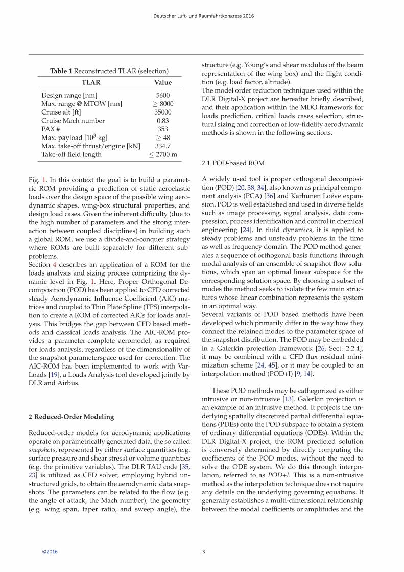
Table 1 Reconstructed TLAR (selection)

TLAR Value

Design range [nm] 5600Max. range @ MTOW [nm] ≥ 8000Cruise alt [ft] 35000Cruise Mach number 0.83PAX # 353Max. payload [103 kg] ≥ 48Max. take-off thrust/engine [kN] 334.7Take-off field length ≤ 2700 m

Fig. 1. In this context the goal is to build a paramet-ric ROM providing a prediction of static aeroelasticloads over the design space of the possible wing aero-dynamic shapes, wing-box structural properties, anddesign load cases. Given the inherent difficulty (due tothe high number of parameters and the strong inter-action between coupled disciplines) in building sucha global ROM, we use a divide-and-conquer strategywhere ROMs are built separately for different sub-problems.Section 4 describes an application of a ROM for theloads analysis and sizing process comprizing the dy-namic level in Fig. 1. Here, Proper Orthogonal De-composition (POD) has been applied to CFD correctedsteady Aerodynamic Influence Coefficient (AIC) ma-trices and coupled to Thin Plate Spline (TPS) interpola-tion to create a ROM of corrected AICs for loads anal-ysis. This bridges the gap between CFD based meth-ods and classical loads analysis. The AIC-ROM pro-vides a parameter-complete aeromodel, as requiredfor loads analysis, regardless of the dimensionality ofthe snapshot parameterspace used for correction. TheAIC-ROM has been implemented to work with Var-Loads [19], a Loads Analysis tool developed jointly byDLR and Airbus.

2 Reduced-Order Modeling

Reduced-order models for aerodynamic applicationsoperate on parametrically generated data, the so calledsnapshots, represented by either surface quantities (e.g.surface pressure and shear stress) or volume quantities(e.g. the primitive variables). The DLR TAU code [35,23] is utilized as CFD solver, employing hybrid un-structured grids, to obtain the aerodynamic data snap-shots. The parameters can be related to the flow (e.g.the angle of attack, the Mach number), the geometry(e.g. wing span, taper ratio, and sweep angle), the

structure (e.g. Young’s and shear modulus of the beamrepresentation of the wing box) and the flight condi-tion (e.g. load factor, altitude).The model order reduction techniques used within theDLR Digital-X project are hereafter briefly described,and their application within the MDO framework forloads prediction, critical loads cases selection, struc-tural sizing and correction of low-fidelity aerodynamicmethods is shown in the following sections.

2.1 POD-based ROM

A widely used tool is proper orthogonal decomposi-tion (POD) [20, 38, 34], also known as principal compo-nent analysis (PCA) [36] and Karhunen Loeve expan-sion. POD is well established and used in diverse fieldssuch as image processing, signal analysis, data com-pression, process identification and control in chemicalengineering [24]. In fluid dynamics, it is applied tosteady problems and unsteady problems in the timeas well as frequency domain. The POD method gener-ates a sequence of orthogonal basis functions throughmodal analysis of an ensemble of snapshot flow solu-tions, which span an optimal linear subspace for thecorresponding solution space. By choosing a subset ofmodes the method seeks to isolate the few main struc-tures whose linear combination represents the systemin an optimal way.Several variants of POD based methods have beendeveloped which primarily differ in the way how theyconnect the retained modes to the parameter space ofthe snapshot distribution. The POD may be embeddedin a Galerkin projection framework [26, Sect. 2.2.4],it may be combined with a CFD flux residual mini-mization scheme [24, 45], or it may be coupled to aninterpolation method (POD+I) [9, 14].

These POD methods may be cathegorized as eitherintrusive or non-intrusive [13]. Galerkin projection isan example of an intrusive method. It projects the un-derlying spatially discretized partial differential equa-tions (PDEs) onto the POD subspace to obtain a systemof ordinary differential equations (ODEs). Within theDLR Digital-X project, the ROM predicted solutionis conversely determined by directly computing thecoefficients of the POD modes, without the need tosolve the ODE system. We do this through interpo-lation, referred to as POD+I. This is a non-intrusivemethod as the interpolation technique does not requireany details on the underlying governing equations. Itgenerally establishes a multi-dimensional relationshipbetween the modal coefficients or amplitudes and the


3©2016

parameter space, e.g. by fitting a radial basis functionnetwork in the modal space to the set of snapshotpoints in the parameter space. This has the advantageof simplicity of implementation and independence ofthe complexity of the system and source of the modesbeing processed, which allows for application to mul-tidisciplinary problems and the combination of differ-ent data sources such as CFD and experimental testresults.The main disadvantage of non-intrusive POD meth-ods stems from their reliance on interpolation tech-niques to accurately reproduce the possibly very non-linear response surfaces of the modal coefficients. In-trusive POD methods do better in this respect. Withinthe DLR Digital-X project, we do this through an op-timization problem which minimizes the residual ofthe underlying equations, which will be referred to asPOD+LSQ.

2.2 Isomap-based ROM

The linear nature of the POD makes the method at-tractive but also is the source of its restriction. Highlynon-linear flow phenomena, such as shocks, are ofteninsufficiently reproduced, because of the underlyingassumption that the full-order CFD flow solution liein a low-dimensional linear subspace. An approachto improve the fidelity of linear ROMs is to subtitutethe POD with a nonlinear manifold learning (ML) [10,27, 30, 7], or, more generally, dimensionality reduction(DR) technique. This shifts the burden of reproducingcomplex flow phenomena from the interpolation to theDR technique, by assuming that full-order data lieson a nonlinear manifold of low-dimension. Such tech-niques try to solve the so-called embedding problem.In general, this is an ill-posed problem, because neitherthe geometry of the data nor the intrinsic dimension-ality is known.Within the DLR Digital-X project, the Isomap [37]method, which is a nonlinear DR method based onmulti-dimensional scaling (MDS) [28], is employed toextract low-dimensional structures hidden in a givenhigh-dimensional data set.

The Isomap method only provides a mapping fromthe high-dimensional input space onto a lower-dimen-sional embedding space for a fixed finite set of givensnapshots. For any ROM of the Navier-Stokes equa-tions, however, it is an essential requirement that theapproximate reduced-order flow solutions are of thesame type and dimension as the full-order CFD snap-shots. Hence, once the set of low-dimensional vectorsis obtained, a back-mapping from the reduced-order

embedding to the high-dimensional solution space ismandatory.Coupled with an interpolation model formulated be-tween the parameter space and the low-dimensionalspace, a ROM is obtained which is capable of predict-ing full-order solutions at untried parameter combina-tions. This method will be referred to as Isomap+I.Furthermore, another back-mapping from the low-dimensional space to the high-dimensional space maybe performed based on the residual optimization. Itsobjective is to obtain a CFD-enhanced prediction byminimizing the discretized flux residual of the inter-polated solution. This method will be referred to asIsomap+LSQ.

3 Reduced-Order Models for Static Aeroelastic

Loads

In this section we present a reduced order modelingprocess for computing static aeroelastic loads, to beused in the framework of high-fidelity MDO [32] andsizing process as shown in Fig. 3. The method consistsof building a ROM from static aeroelastic solutionscomputed for different sets of parameters. Such so-lutions are collected in a snapshot matrix, to which aPOD [9] or an Isomap [37] embedding is applied in or-der to get a (linear or nonlinear) low-dimensional sub-space. A reduced order model, either POD-based orIsomap-based, is built from static aeroelastic solutionscomputed for different sets of parameters like, e.g.,flight conditions (altitude, number of Mach, load fac-tor), flight configurations (payload mass, fuel mass),geometrical parameters (wing planform parameters asaspect ratio, taper ratio, swept angle, and the twistangle for selected airfoil sections) and structural prop-erties (wing-box stiffness and mass). The parameterspace is sampled using Design of Experiment (DoE)techniques [12].

However, the integrated nature of the MDO pro-cess involves complex interactions between the differ-ent disciplines, which are difficult to be representedwith a single global ROM, if not at the expense of acostly sampling of the whole paramater design spacewith multidisciplinary high-fidelity simulations. Be-ing understood that such a global ROM may be de-vised and sought in future works and projects, here-after an efficient approach to manage this complexityis shown, where a divide-and-conquer strategy is ap-plyed and the MDO is decomposed in sub-processes,for which small parametric ROMs can be easier gener-ated separately and used for fast system-level analysis.

First, section 3.1 describes how to construct a ROMof coupled, static aeroelastic solutions for a given (flex-


4©2016

Aeroelastic Model

Structural Model

Sizing process

Wing Shape Optimizer

Flight Performances

Aerodynamic Model

Mesh Deformation

Compute flow solution

Forces

DisplacementsBuild/update

model

Structural Mass

Compute deformations

Thickness /Section Area

Optimizer

Geometry (planform, profiles)

Flight conditions and

critical load cases

Flight performances data and constraints

(lift/drag)

Design Cases

ROM parameters

ROM parameters

ROM snapshots

Reduced Order Model for LoadsROM loads

prediction for initial sizing and MDO

ROM parameters

Conceptual Design

ROM for rapid critical load cases

identification

Mission requirements and

objectives

Aircraft Configuration Topology, Architecture

and Layout

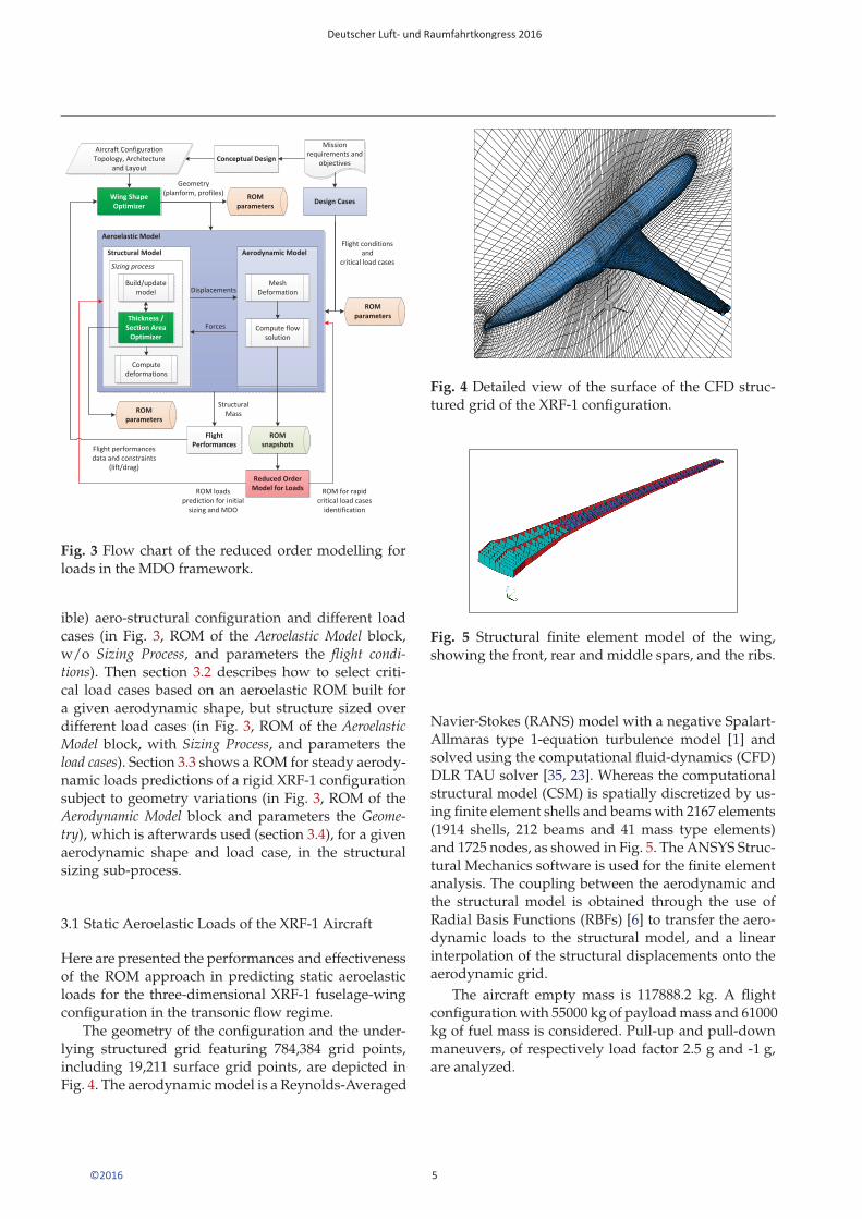
Fig. 3 Flow chart of the reduced order modelling forloads in the MDO framework.

ible) aero-structural configuration and different loadcases (in Fig. 3, ROM of the Aeroelastic Model block,w/o Sizing Process, and parameters the flight condi-tions). Then section 3.2 describes how to select criti-cal load cases based on an aeroelastic ROM built fora given aerodynamic shape, but structure sized overdifferent load cases (in Fig. 3, ROM of the AeroelasticModel block, with Sizing Process, and parameters theload cases). Section 3.3 shows a ROM for steady aerody-namic loads predictions of a rigid XRF-1 configurationsubject to geometry variations (in Fig. 3, ROM of theAerodynamic Model block and parameters the Geome-try), which is afterwards used (section 3.4), for a givenaerodynamic shape and load case, in the structuralsizing sub-process.

3.1 Static Aeroelastic Loads of the XRF-1 Aircraft

Here are presented the performances and effectivenessof the ROM approach in predicting static aeroelasticloads for the three-dimensional XRF-1 fuselage-wingconfiguration in the transonic flow regime.

The geometry of the configuration and the under-lying structured grid featuring 784,384 grid points,including 19,211 surface grid points, are depicted inFig. 4. The aerodynamic model is a Reynolds-Averaged

XY

Z

Fig. 4 Detailed view of the surface of the CFD struc-tured grid of the XRF-1 configuration.

Fig. 5 Structural finite element model of the wing,showing the front, rear and middle spars, and the ribs.

Navier-Stokes (RANS) model with a negative Spalart-Allmaras type 1-equation turbulence model [1] andsolved using the computational fluid-dynamics (CFD)DLR TAU solver [35, 23]. Whereas the computationalstructural model (CSM) is spatially discretized by us-ing finite element shells and beams with 2167 elements(1914 shells, 212 beams and 41 mass type elements)and 1725 nodes, as showed in Fig. 5. The ANSYS Struc-tural Mechanics software is used for the finite elementanalysis. The coupling between the aerodynamic andthe structural model is obtained through the use ofRadial Basis Functions (RBFs) [6] to transfer the aero-dynamic loads to the structural model, and a linearinterpolation of the structural displacements onto theaerodynamic grid.

The aircraft empty mass is 117888.2 kg. A flightconfiguration with 55000 kg of payload mass and 61000kg of fuel mass is considered. Pull-up and pull-downmaneuvers, of respectively load factor 2.5 g and -1 g,are analyzed.


5©2016

The computation of the coupled flow-structure so-lutions were performed in parallel on the DLR C2A2S2E-2 cluster using 2 nodes1 with 24 cores. Computing afree-flight coupled CFD (TAU) - CSM (ANSYS) staticaeroelastic solution took an average2 of 2430 wall-clock seconds.

The aeroelastic equilibrium and the trim correc-tion3 are computed independently with two nestedloop. Each iteration to find the static aeroelastic equi-librium (outer loop) involves interpolation of the dis-placements from the CSM to the CFD mesh, defor-mation of the CFD mesh using RBFs, computation ofthe flow solution (with inner loop target CL trimmingstrategy), interpolation of the forces from the CFDmodel to the CSM mesh, and computation of the struc-ture solution.

An average of 4 coupling outer iterations are nec-essary for the static aeroelastic convergence. In eachof these coupled iterations, the solution of the trim isobained through a target CL strategy, where the angleof attack is determined so as to provide a lift balanc-ing the aircraft weight and the inertial force due to agiven load factor. Here the CFD subsystem is solved byfirst using a minimum iteration strategy, running 3500iterations, followed by a minimum residual strategy,where the density residual is converged by four ordersof magnitude at the initial coupled iteration, up to sixorders of magnitude proceeding with the coupled it-erations. In the minimum residual strategy a maximalinner iteration number of 9950 is anyhow set-up.

For the test case presented, the ROM is parametrizedonly upon flight conditions, i.e., altitude and Machnumber. Choosing suitable flight conditions and con-figurations parameter combinations for the snapshotcomputation is a very important issue in building theROM. In this case, static aeroelastic high-fidelity simu-lations have been performed (offline) for a Mach num-ber ranging from 0.65 to 0.82, and an altitude between0 m and 5000 m. The payload and fuel masses arekept fixed. The sample points are computed using afull factorial design strategy over the Mach number

1Intel R© Xeon R© E5-2695 v2 Processors (30M Cache, 2.40GHz, 12 Cores)

2Based on the effectively computed reference solutions, i.e.without taking into account the not converged simulations.

3It must be noted that the aircraft model is missing thehorizontal tail plane (HTP). Therefore, the equilibrium conditionis applied only in the vertical translation direction. The aircraftpitching moment will not be trimmed, and the resulting wing liftwill therefore only balance the inertial loads and not the (usual)negative lift of the HTP. Despite only the vertical equilibriumis considered, the coupled procedure still offers fluid-structuresnapshots suitable to verify the soundness of the ROM capabil-ity in predicting approximate solutions.

Mach

altit

ude

[m]

0.6 0.65 0.7 0.75 0.8 0.850

1000

2000

3000

4000

5000

DoE SamplesPrediction Points

Fig. 6 Design of experiment samples and predictionpoints.

range between 0.65 and 0.80, with additional pointsalong Mach 0.82. Only the converged solutions, i.e. 22snapshots, have been taken into account in the ROMgeneration procedure. The ROM is realized througha POD of the high-fidelity snapshots together witha Thin Plate Spline (TPS) method interpolating thePOD coefficients to get the predicted aeroelastic so-lution (i.e. the surface pressure, the skin friction andthe structural displacement). All the POD modes havebeen reteined. The performances of the ROM approachare evaluated at flight conditions with Mach number0.81, for different altitudes. The prediction points andthe DoE sample points are shown in Fig. 6.

Before computing the ROM predictions, a leave-1-out cross-validation strategy has been performed tounderstand if the set of sample points were enoughto cover the parameter space. Therefore, following thisstrategy, alternately one of the high-fidelity snapshotsof the DoE sample set has been left out from the ROMgeneration procedure (which is then built using theremaining 21 DoE sample snapshots as the training set,retaining all the 21 POD modes). In the correspondingflight condition of the left-out snapshot (i.e. the valida-tion point) the ROM prediction has been performed.This prediction has been compared to the high-fidelitycomputation in terms of aerodynamic coefficients.

It must be noted that the inputs of the reduced or-der model are only the Mach number and the altitude.Therefore the ROM aeroelastic prediction is not asso-ciated with any angle of attack. The only informationabout the freestream boundary condition is related to


6©2016

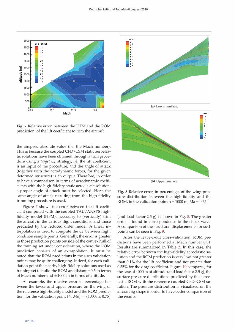
Fig. 7 Relative error, between the HFM and the ROMprediction, of the lift coefficient to trim the aircraft.

the airspeed absolute value (i.e. the Mach number).This is because the coupled CFD/CSM static aeroelas-tic solutions have been obtained through a trim proce-dure using a target CL strategy, i.e. the lift coefficientis an input of the procedure, and the angle of attack(together with the aerodynamic forces, for the givendeformed structure) is an output. Therefore, in orderto have a comparison in terms of aerodynamic coeffi-cients with the high-fidelity static aeroelastic solution,a proper angle of attack must be selected. Here, thesame angle of attack resulting from the high-fidelitytrimming procedure is used.

Figure 7 shows the error between the lift coeffi-cient computed with the coupled TAU/ANSYS high-fidelity model (HFM), necessary to (vertically) trimthe aircraft in the various flight conditions, and thosepredicted by the reduced order model. A linear in-terpolation is used to compute the CL between flightcondition sample points. Generally, the error is greaterin those prediction points outside of the convex hull ofthe training set under consideration, where the ROMprediction consists of an extrapolation. It must benoted that the ROM predictions in the such validationpoints may be quite challenging. Indeed, for each vali-dation point the nearby high-fidelity solutions used astraining set to build the ROM are distant ±0.5 in termsof Mach number and ±1000 m in terms of altitude.

As example, the relative error in percentage be-tween the lower and upper pressure on the wing ofthe reference high-fidelity model and the ROM predic-tion, for the validation point (h, Ma) = (1000 m, 0.75)

(a) Lower surface.

(b) Upper surface.

Fig. 8 Relative error, in percentage, of the wing pres-sure distribution between the high-fidelity and theROM, in the validation point h = 1000 m, Ma = 0.75.

(and load factor 2.5 g) is shown in Fig. 8. The greatererror is found in correspondence to the shock wave.A comparison of the structural displacements for suchpoints can be seen in Fig. 9.

After the leave-1-out cross-validation, ROM pre-dictions have been performed at Mach number 0.81.Results are summarized in Table 2. In this case, therelative error between the high-fidelity aeroelastic so-lution and the ROM prediction is very low, not greaterthan 0.1% for the lift coefficient and not greater than0.35% for the drag coefficient. Figure 10 compares, forthe case of 4000 m of altitude (and load factor 2.5 g), thesurface pressure distributions predicted by the aeroe-lastic ROM with the reference coupled CFD–CSM so-lution. The pressure distribution is visualized on theaircraft jig shape in order to have better comparison ofthe results.


7©2016

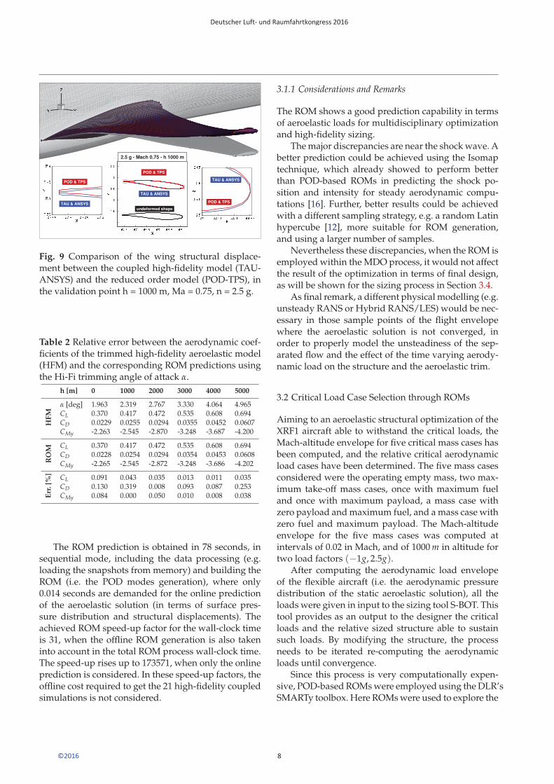
Fig. 9 Comparison of the wing structural displace-ment between the coupled high-fidelity model (TAU-ANSYS) and the reduced order model (POD-TPS), inthe validation point h = 1000 m, Ma = 0.75, n = 2.5 g.

Table 2 Relative error between the aerodynamic coef-ficients of the trimmed high-fidelity aeroelastic model(HFM) and the corresponding ROM predictions usingthe Hi-Fi trimming angle of attack α.

h [m] 0 1000 2000 3000 4000 5000

HF

M

α [deg] 1.963 2.319 2.767 3.330 4.064 4.965CL 0.370 0.417 0.472 0.535 0.608 0.694CD 0.0229 0.0255 0.0294 0.0355 0.0452 0.0607CMy -2.263 -2.545 -2.870 -3.248 -3.687 -4.200

RO

M

CL 0.370 0.417 0.472 0.535 0.608 0.694CD 0.0228 0.0254 0.0294 0.0354 0.0453 0.0608CMy -2.265 -2.545 -2.872 -3.248 -3.686 -4.202

Err

.[%

] CL 0.091 0.043 0.035 0.013 0.011 0.035CD 0.130 0.319 0.008 0.093 0.087 0.253CMy 0.084 0.000 0.050 0.010 0.008 0.038

The ROM prediction is obtained in 78 seconds, insequential mode, including the data processing (e.g.loading the snapshots from memory) and building theROM (i.e. the POD modes generation), where only0.014 seconds are demanded for the online predictionof the aeroelastic solution (in terms of surface pres-sure distribution and structural displacements). Theachieved ROM speed-up factor for the wall-clock timeis 31, when the offline ROM generation is also takeninto account in the total ROM process wall-clock time.The speed-up rises up to 173571, when only the onlineprediction is considered. In these speed-up factors, theoffline cost required to get the 21 high-fidelity coupledsimulations is not considered.

3.1.1 Considerations and Remarks

The ROM shows a good prediction capability in termsof aeroelastic loads for multidisciplinary optimizationand high-fidelity sizing.

The major discrepancies are near the shock wave. Abetter prediction could be achieved using the Isomaptechnique, which already showed to perform betterthan POD-based ROMs in predicting the shock po-sition and intensity for steady aerodynamic compu-tations [16]. Further, better results could be achievedwith a different sampling strategy, e.g. a random Latinhypercube [12], more suitable for ROM generation,and using a larger number of samples.

Nevertheless these discrepancies, when the ROM isemployed within the MDO process, it would not affectthe result of the optimization in terms of final design,as will be shown for the sizing process in Section 3.4.

As final remark, a different physical modelling (e.g.unsteady RANS or Hybrid RANS/LES) would be nec-essary in those sample points of the flight envelopewhere the aeroelastic solution is not converged, inorder to properly model the unsteadiness of the sep-arated flow and the effect of the time varying aerody-namic load on the structure and the aeroelastic trim.

3.2 Critical Load Case Selection through ROMs

Aiming to an aeroelastic structural optimization of theXRF1 aircraft able to withstand the critical loads, theMach-altitude envelope for five critical mass cases hasbeen computed, and the relative critical aerodynamicload cases have been determined. The five mass casesconsidered were the operating empty mass, two max-imum take-off mass cases, once with maximum fueland once with maximum payload, a mass case withzero payload and maximum fuel, and a mass case withzero fuel and maximum payload. The Mach-altitudeenvelope for the five mass cases was computed atintervals of 0.02 in Mach, and of 1000 m in altitude fortwo load factors (−1g, 2.5g).

After computing the aerodynamic load envelopeof the flexible aircraft (i.e. the aerodynamic pressuredistribution of the static aeroelastic solution), all theloads were given in input to the sizing tool S-BOT. Thistool provides as an output to the designer the criticalloads and the relative sized structure able to sustainsuch loads. By modifying the structure, the processneeds to be iterated re-computing the aerodynamicloads until convergence.

Since this process is very computationally expen-sive, POD-based ROMs were employed using the DLR’sSMARTy toolbox. Here ROMs were used to explore the


8©2016

x/c

Cp

0 0.2 0.4 0.6 0.8 1

-1.5

-1

-0.5

0

0.5

y/b = 75%

Cp

0 0.2 0.4 0.6 0.8 1

-1.5

-1

-0.5

0

0.5

y/b = 50%

x/c

Cp

0 0.2 0.4 0.6 0.8 1

-1.5

-1

-0.5

0

0.5

HiFi: TAU & ANSYSROM: POD & TPS

y/b = 25%

X

Y Z

Cp0.60.40.20

-0.2-0.4-0.6-0.8-1

y/b = 25%

y/b = 50%

y/b = 75%

XY

ZCp10.80.60.40.20

-0.2-0.4-0.6-0.8-1

Fig. 10 Comparison of the pressure distribution at the 25%, 50% and 70% spanwise airfoil sections, for Mach 0.81and altitude 4000 m.

parameter space with a finer sampling at in-betweenaltitudes. The (in-between altitudes) ROM predictedaeroelastic loads are sent to the sizing tool, which de-termines if the loads are critical. Whenever a newlypredicted aeroelastic load is found to be potentiallycritical, the corresponding load case is recomputedwith the high-fidelity coupled CFD-CSM methods andchecked with the sizing tool if it is really critical or not.

As an example, two of the five critical mass caseswere used to generate 400 sized high-fidelity aeroelas-tic snapshots. A parametric reduced-order model hasbeen generated using such snapshots, and then used tocompute 360 additional loads predictions. Of these 360predictions, 3 were found to be additional candidatesfor critical load cases, and by computing them with thehigh-fidelity tools one case was found to be actuallycritical. Figure 11 shows the complete aerodynamicload case identification process.

This process guarantees an efficient search and se-lection for new critical load cases. However, it shouldbe pointed out that the prediction capability of theROMs depends on the high fidelity snapshots usedto generate them. Reduced-order models after all are

SizingCFD Structure

ROMs Sizing

400 Snapshots

Load cases

360 predictions

Fig. 11 The load case identification process.

nothing else than a linear combination of the approx-imation of such snapshots. Therefore it may possiblethat the ROMs can fail to provide additional candi-dates for the critical load cases, which might turn outto be critical for the sizing process if computed withhigh-fidelity methods.


9©2016

Fig. 12 Front view of the XRF-1. Twists are performedat five section cuts depicted by the black lines on thewing. The left and the right wing show the maximumtwists in different rotation directions.

3.3 Parametric ROMs for Aero-Data in MDO

This section shows the use of parametric, Isomap-based, reduced-order models for the prediciton of theaerodynamic loads of the rigid XRF-1 aircraft, subjectto wing geometry variations. The Mach number andthe Reynolds number are here fixed respectively atMa = 0.83 and Re ≈ 43.4 · 106. Furthermore, a targetlift coefficient of Cl = 0.5 is prescribed. The twist offive wing sections are used as parameters of the ROM.The wing sections positions and the maximum twist indifferent rotation directions are shown in Fig. 12.

An adaptive sampling with a hybrid error (HYE)strategy [15] is employed to generate a sampling ofthe high-dimensional data manifold W . The data man-ifold W is given by varying the five twist parame-ters of the configuration in the parameter space P =[−0.2, 0.2] × [−2, 2] × [−3, 3] × [−2, 2] × [−1, 1] ⊂ R5,where the intervals from left to right correspond tothe twist sections from fuselage to tip. A total of 100viscous flow solution snapshots have been computedwith the TAU RANS solver, whereby the normalizeddensity residual is reduced by six orders of magnitudefor each solution. Since a target lift coefficient of Cl =0.5 is aimed at, the angle of attack α varies during theCFD simulation until the target lift is matched.

The sampling process including the computationof the flow solutions and all further computationswere performed in parallel on the DLR C2A2S2E-2cluster using one node endowed with 128 GB RAMand two Intel R© Xeon R© E5-2695 v2 Processors (30MCache, 2.40 GHz, 12 Cores). Computing a full CFDsolution for this test case took 5393 iterations or 4214CPU seconds on average.

Once the data manifold W = {W1, . . . , W100} ⊂ Wis obtained, with corresponding parameter set P ={p1, . . . , p100} ⊂ P , the Isomap based ROMs pre-dictions are computed at untried points p ∈ P \ P.Such points p were chosen as the centers of the 10simplices with the largest volume of the Delaunay tri-

angulation [33, 4] of P, so as to maximize their distancefrom each p ∈ P. The error at a prediction point p ∈ Pis computed as:

err(Wref(p), W∗(p)) =∑i∈IR

|Wrefi − W∗

i |∑i∈IR

|Wrefi | (1)

being Wref(p) ∈ Rn and W∗(p) ∈ Rn respectively thereference solution and the ROM-based prediction atp ∈ P , and n the product of the number of grid pointsand the number of variables, i. e. n = ngnv.

As will be shown, the results are accurate. Hence,the Isomap based ROMs for aero-data can be exploitedfor a multidisciplinary optimization within the wholeparameter space, saving the costs of computing full-order CFD solutions.

3.3.1 Isomap with Interpolation

The interpolation based ROM makes use only of thesurface snapshots, hence Wi ∈ R19,211. Since fiveparameters are varied, the Isomap algorithm is ap-plied to surface Cp-distribution vectors to compute a5-dimensional embedding consisting of 100 represen-tatives yi ∈ R5. The neighborhood graph is built using87 nearest neighbors, and the back-mapping employesbetween 10 − 20 nearest neighbors.

For comparison purposes, a global POD of the 100full-order surface Cp snapshots is performed, yield-ing a basis consisting of 99 orthonormal POD eigen-mode vectors4 of dimension 19,211. As before, thePOD model is combined with a TPS interpolationscheme [15, 6]. Compared to Isomap+I, where a rep-resentative y∗ ∈ R5 of dimension five has to be in-terpolated to obtain a surface Cp prediction, POD+Iemploys TPS to interpolate the POD coefficient vectora ∈ R99 of much larger dimension.

Isomap+I and POD+I were built in 119 and 0.17CPU seconds, respectively, including the data pro-cessing, setting up the TPS model and, in the caseof Isomap, the computation of the proper number ofnearest neighbors [15]. Although there is a big dif-ference between the building times of Isomap+I andPOD+I, compared to a full CFD calculation the offlinetimes (without the snapshot computations) are negli-gible. The online prediction of a surface solution at anuntried parameter combination p ∈ P \ P took lessthan 0.01 CPU seconds for both ROMs, whereas a fullCFD solution took 4214 CPU seconds on average. Inother words, the predictions of both ROMs are morethan 400,000 times faster than a full CFD solution, butcertainly due to a trade-off of less accuracy.

4The mean of the snapshots is subtracted.


10©2016

Table 3 Errors in terms of equation (1) between theTAU reference surface Cp solutions and the surfaceCp predictions obtained by Isomap+I, Isomap+LSQ,POD+I and POD+LSQ at various parameter combi-nations. The column NN lists the number of nearestneighbors employed by the Isomap based predictionsat each parameter combination p.

p NN Isomap+I Isomap+LSQ POD+I POD+LSQ

1 11 8.5930·10−2 7.1702·10−2 9.4556·10−2 5.9426·10−2

2 16 8.7347·10−2 7.5275·10−2 1.1523·10−1 5.5323·10−2

3 14 7.7126·10−2 7.5143·10−2 9.4977·10−2 6.3302·10−2

4 10 1.0089·10−1 1.3703·10−1 1.3514·10−1 6.4285·10−2

5 20 6.4210·10−2 7.1029·10−2 7.7599·10−2 5.7465·10−2

6 10 7.0431·10−2 9.3372·10−2 7.7246·10−2 5.9561·10−2

7 14 6.7638·10−2 5.1527·10−2 9.1839·10−2 4.4243·10−2

8 10 4.3445·10−2 4.5011·10−2 8.9193·10−2 3.0280·10−2

9 13 5.6208·10−2 4.0005·10−2 7.4482·10−2 2.8970·10−2

10 10 6.3993·10−2 5.9396·10−2 8.7417·10−2 4.1372·10−2

The resulting surface Cp-distributions predicted byIsomap+I and POD+I for various parameter combina-tions are compared to the corresponding TAU refer-ence solutions. The corresponding errors in terms ofequation (1) for the predictions points are given inTable 3. The Isomap+I predictions feature a smallererror than the POD+I predictions. An example of theROM aerodynamic loads predictions (in terms of sur-face Cp-distribution) for an untried parameter combi-nation (p8 of Table 3) is given in Fig. 13. The Isomap+Iprediction matches the surface Cp-distribution of theTAU reference solution quiet accurately. The POD+Iprediction also yields accurate predictions, but the Cp-distribution between the first two sections differs fromthe reference solution.

Of course, due to the complexity of the test case,where arbitrary twists at the five sections of the wingare analysed, there could be cases where the ROM pre-dictions are less accurate, so leading to bigger errors(see e.g. the parameter combination p4 in Table 3).

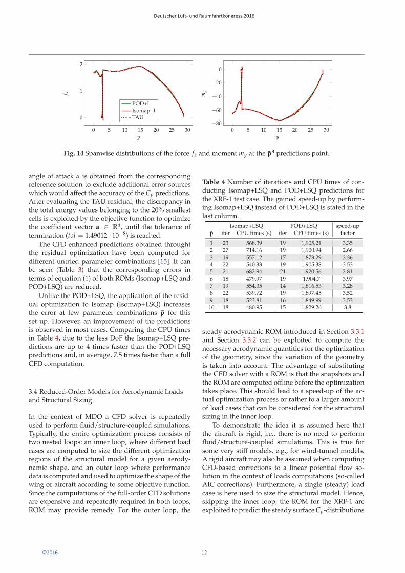
The spanwise distributions of the partial force fzand the partial moment my, calculated via AeroForce [41],are shown for the parameter combination p8 in Fig. 14.As it can be seen, there is a good match between theforce and moment distributions of the reference solu-tion and those of the ROM prediction.

3.3.2 Isomap with Residual Optimization

The interpolation-based Isomap and POD coefficientscan be then exploited as starting values for the resid-ual based ROM [15]. The unconstrained optimizationproblems are solved now. To optimize the coefficientsof an Isomap or POD based prediction, the Levenberg-Marquardt algorithm [29, 42] with additional Broy-

Fig. 13 Prediction of the surface Cp-distribution of theXRF-1 by Isomap+I and POD+I at an untried param-eter combination p8 ∈ P \ P. The four section cuts,ordered line by line from left to right, correspond tothe twist sections from fuselage to tip.

den’s rank one updates of the Jacobian is applied tothe unconstrained optimization problems [15].

All primitive variables plus the Cp-distribution aretaken into account, leading to a set of snapshots W ⊂Rn, n = ng · nv = 6, 275, 072. Hence, Isomap+LSQ andPOD+LSQ are based on 100 snapshots of dimensionn = 6, 275, 072, increasing the building time of thePOD based ROM to 117 CPU seconds. The costs ofIsomap+LSQ (119 CPU seconds) remains unaffected ofthe new data set, as only the surface Cp-distribution isexploited to compute the embedding.

The residual has to be evaluated with proper bound-ary conditions Ma and α, which are not specified bythe varied parameters. While the Mach number Ma isfixed, the angle of attack α varies for each flow solu-tions to ensure the specified target Cl value. Here, the


11©2016

0 5 10 15 20 25 30

0

1

2

y

f z

POD+IIsomap+ITAU

0 5 10 15 20 25 30−80

−60

−40

−20

0

y

my

Fig. 14 Spanwise distributions of the force fz and moment my at the p8 predictions point.

angle of attack α is obtained from the correspondingreference solution to exclude additional error sourceswhich would affect the accuracy of the Cp predictions.After evaluating the TAU residual, the discrepancy inthe total energy values belonging to the 20% smallestcells is exploited by the objective function to optimizethe coefficient vector a ∈ Rd, until the tolerance oftermination (tol = 1.49012 · 10−8) is reached.

The CFD enhanced predictions obtained throughtthe residual optimization have been computed fordifferent untried parameter combinations [15]. It canbe seen (Table 3) that the corresponding errors interms of equation (1) of both ROMs (Isomap+LSQ andPOD+LSQ) are reduced.

Unlike the POD+LSQ, the application of the resid-ual optimization to Isomap (Isomap+LSQ) increasesthe error at few parameter combinations p for thisset up. However, an improvement of the predictionsis observed in most cases. Comparing the CPU timesin Table 4, due to the less DoF the Isomap+LSQ pre-dictions are up to 4 times faster than the POD+LSQpredictions and, in average, 7.5 times faster than a fullCFD computation.

3.4 Reduced-Order Models for Aerodynamic Loadsand Structural Sizing

In the context of MDO a CFD solver is repeatedlyused to perform fluid/structure-coupled simulations.Typically, the entire optimization process consists oftwo nested loops: an inner loop, where different loadcases are computed to size the different optimizationregions of the structural model for a given aerody-namic shape, and an outer loop where performancedata is computed and used to optimize the shape of thewing or aircraft according to some objective function.Since the computations of the full-order CFD solutionsare expensive and repeatedly required in both loops,ROM may provide remedy. For the outer loop, the

Table 4 Number of iterations and CPU times of con-ducting Isomap+LSQ and POD+LSQ predictions forthe XRF-1 test case. The gained speed-up by perform-ing Isomap+LSQ instead of POD+LSQ is stated in thelast column.

Isomap+LSQ POD+LSQ speed-upp iter CPU times (s) iter CPU times (s) factor

1 23 568.39 19 1,905.21 3.352 27 714.16 19 1,900.94 2.663 19 557.12 17 1,873.29 3.364 22 540.33 19 1,905.38 3.535 21 682.94 21 1,920.56 2.816 18 479.97 19 1,904.7 3.977 19 554.35 14 1,816.53 3.288 22 539.72 19 1,897.45 3.529 18 523.81 16 1,849.99 3.5310 18 480.95 15 1,829.26 3.8

steady aerodynamic ROM introduced in Section 3.3.1and Section 3.3.2 can be exploited to compute thenecessary aerodynamic quantities for the optimizationof the geometry, since the variation of the geometryis taken into account. The advantage of substitutingthe CFD solver with a ROM is that the snapshots andthe ROM are computed offline before the optimizationtakes place. This should lead to a speed-up of the ac-tual optimization process or rather to a larger amountof load cases that can be considered for the structuralsizing in the inner loop.

To demonstrate the idea it is assumed here thatthe aircraft is rigid, i.e., there is no need to performfluid/structure-coupled simulations. This is true forsome very stiff models, e.g., for wind-tunnel models.A rigid aircraft may also be assumed when computingCFD-based corrections to a linear potential flow so-lution in the context of loads computations (so-calledAIC corrections). Furthermore, a single (steady) loadcase is here used to size the structural model. Hence,skipping the inner loop, the ROM for the XRF-1 areexploited to predict the steady surface Cp-distributions


12©2016

240 250 260 270 280 290 300 310 320 330 340 350

0

1

2·10−2

Opt region

Thic

knes

s(m

)

TAUIsomap+I

240 250 260 270 280 290 300 310 320 330 340 350

0

1

2·10−2

Opt region

Thic

knes

s(m

)

TAUPOD+I

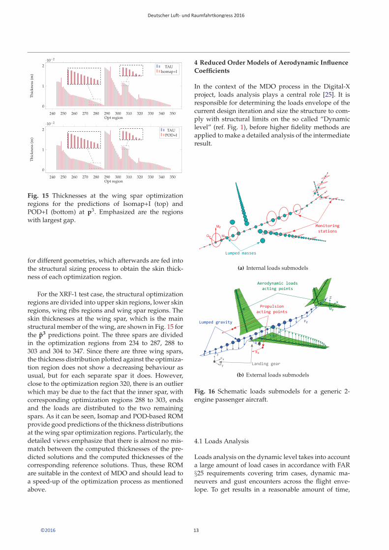
Fig. 15 Thicknesses at the wing spar optimizationregions for the predictions of Isomap+I (top) andPOD+I (bottom) at p3. Emphasized are the regionswith largest gap.

for different geometries, which afterwards are fed intothe structural sizing process to obtain the skin thick-ness of each optimization region.

For the XRF-1 test case, the structural optimizationregions are divided into upper skin regions, lower skinregions, wing ribs regions and wing spar regions. Theskin thicknesses at the wing spar, which is the mainstructural member of the wing, are shown in Fig. 15 forthe p3 predictions point. The three spars are dividedin the optimization regions from 234 to 287, 288 to303 and 304 to 347. Since there are three wing spars,the thickness distribution plotted against the optimiza-tion region does not show a decreasing behaviour asusual, but for each separate spar it does. However,close to the optimization region 320, there is an outlierwhich may be due to the fact that the inner spar, withcorresponding optimization regions 288 to 303, endsand the loads are distributed to the two remainingspars. As it can be seen, Isomap and POD-based ROMprovide good predictions of the thickness distributionsat the wing spar optimization regions. Particularly, thedetailed views emphasize that there is almost no mis-match between the computed thicknesses of the pre-dicted solutions and the computed thicknesses of thecorresponding reference solutions. Thus, these ROMare suitable in the context of MDO and should lead toa speed-up of the optimization process as mentionedabove.

4 Reduced Order Models of Aerodynamic Influence

Coefficients

In the context of the MDO process in the Digital-Xproject, loads analysis plays a central role [25]. It isresponsible for determining the loads envelope of thecurrent design iteration and size the structure to com-ply with structural limits on the so called “Dynamiclevel” (ref. Fig. 1), before higher fidelity methods areapplied to make a detailed analysis of the intermediateresult.

(a) Internal loads submodels

(b) External loads submodels

Fig. 16 Schematic loads submodels for a generic 2-engine passenger aircraft.

4.1 Loads Analysis

Loads analysis on the dynamic level takes into accounta large amount of load cases in accordance with FAR§25 requirements covering trim cases, dynamic ma-neuvers and gust encounters across the flight enve-lope. To get results in a reasonable amount of time,


13©2016

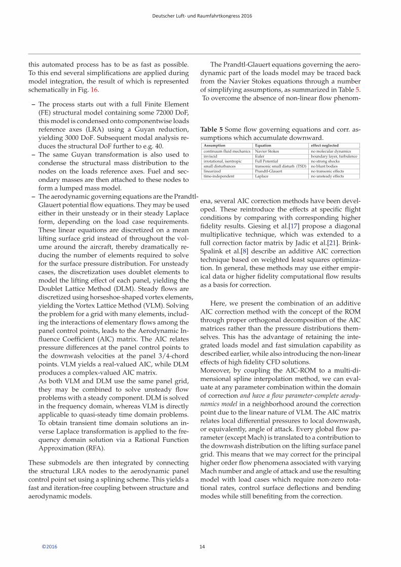
this automated process has to be as fast as possible.To this end several simplifications are applied duringmodel integration, the result of which is representedschematically in Fig. 16.

– The process starts out with a full Finite Element(FE) structural model containing some 72000 DoF,this model is condensed onto componentwise loadsreference axes (LRA) using a Guyan reduction,yielding 3000 DoF. Subsequent modal analysis re-duces the structural DoF further to e.g. 40.

– The same Guyan transformation is also used tocondense the structural mass distribution to thenodes on the loads reference axes. Fuel and sec-ondary masses are then attached to these nodes toform a lumped mass model.

– The aerodynamic governing equations are the Prandtl-Glauert potential flow equations. They may be usedeither in their unsteady or in their steady Laplaceform, depending on the load case requirements.These linear equations are discretized on a meanlifting surface grid instead of throughout the vol-ume around the aircraft, thereby dramatically re-ducing the number of elements required to solvefor the surface pressure distribution. For unsteadycases, the discretization uses doublet elements tomodel the lifting effect of each panel, yielding theDoublet Lattice Method (DLM). Steady flows arediscretized using horseshoe-shaped vortex elements,yielding the Vortex Lattice Method (VLM). Solvingthe problem for a grid with many elements, includ-ing the interactions of elementary flows among thepanel control points, leads to the Aerodynamic In-fluence Coefficient (AIC) matrix. The AIC relatespressure differences at the panel control points tothe downwash velocities at the panel 3/4-chordpoints. VLM yields a real-valued AIC, while DLMproduces a complex-valued AIC matrix.As both VLM and DLM use the same panel grid,they may be combined to solve unsteady flowproblems with a steady component. DLM is solvedin the frequency domain, whereas VLM is directlyapplicable to quasi-steady time domain problems.To obtain transient time domain solutions an in-verse Laplace transformation is applied to the fre-quency domain solution via a Rational FunctionApproximation (RFA).

These submodels are then integrated by connectingthe structural LRA nodes to the aerodynamic panelcontrol point set using a splining scheme. This yields afast and iteration-free coupling between structure andaerodynamic models.

The Prandtl-Glauert equations governing the aero-dynamic part of the loads model may be traced backfrom the Navier Stokes equations through a numberof simplifying assumptions, as summarized in Table 5.To overcome the absence of non-linear flow phenom-

Table 5 Some flow governing equations and corr. as-sumptions which accumulate downward.

Assumption Equation effect neglected

continuum fluid mechanics Navier Stokes no molecular dynamicsinviscid Euler boundary layer, turbulenceirrotational, isentropic Full Potential no strong shockssmall disturbances transonic small disturb. (TSD) no blunt bodieslinearized Prandtl-Glauert no transonic effectstime-independent Laplace no unsteady effects

ena, several AIC correction methods have been devel-oped. These reintroduce the effects at specific flightconditions by comparing with corresponding higherfidelity results. Giesing et al.[17] propose a diagonalmultiplicative technique, which was extended to afull correction factor matrix by Jadic et al.[21]. Brink-Spalink et al.[8] describe an additive AIC correctiontechnique based on weighted least squares optimiza-tion. In general, these methods may use either empir-ical data or higher fidelity computational flow resultsas a basis for correction.

Here, we present the combination of an additiveAIC correction method with the concept of the ROMthrough proper orthogonal decomposition of the AICmatrices rather than the pressure distributions them-selves. This has the advantage of retaining the inte-grated loads model and fast simulation capability asdescribed earlier, while also introducing the non-lineareffects of high fidelity CFD solutions.Moreover, by coupling the AIC-ROM to a multi-di-mensional spline interpolation method, we can eval-uate at any parameter combination within the domainof correction and have a flow parameter-complete aerody-namics model in a neighborhood around the correctionpoint due to the linear nature of VLM. The AIC matrixrelates local differential pressures to local downwash,or equivalently, angle of attack. Every global flow pa-rameter (except Mach) is translated to a contribution tothe downwash distribution on the lifting surface panelgrid. This means that we may correct for the principalhigher order flow phenomena associated with varyingMach number and angle of attack and use the resultingmodel with load cases which require non-zero rota-tional rates, control surface deflections and bendingmodes while still benefiting from the correction.


14©2016

4.2 Surface Geometry Mapping

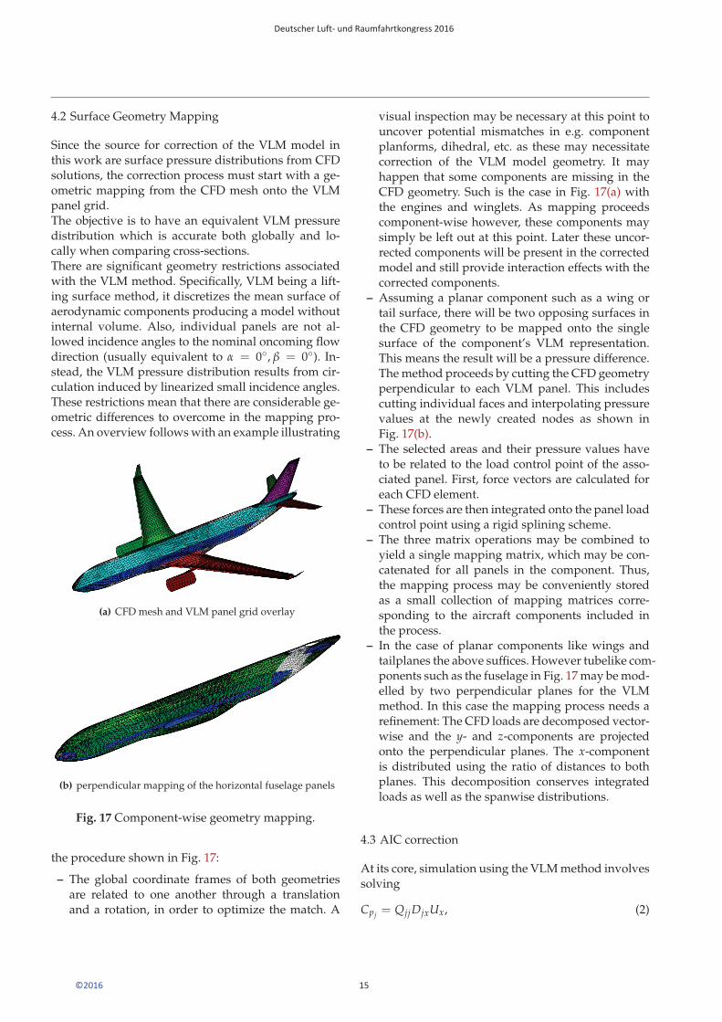
Since the source for correction of the VLM model inthis work are surface pressure distributions from CFDsolutions, the correction process must start with a ge-ometric mapping from the CFD mesh onto the VLMpanel grid.The objective is to have an equivalent VLM pressuredistribution which is accurate both globally and lo-cally when comparing cross-sections.There are significant geometry restrictions associatedwith the VLM method. Specifically, VLM being a lift-ing surface method, it discretizes the mean surface ofaerodynamic components producing a model withoutinternal volume. Also, individual panels are not al-lowed incidence angles to the nominal oncoming flowdirection (usually equivalent to α = 0◦, β = 0◦). In-stead, the VLM pressure distribution results from cir-culation induced by linearized small incidence angles.These restrictions mean that there are considerable ge-ometric differences to overcome in the mapping pro-cess. An overview follows with an example illustrating

(a) CFD mesh and VLM panel grid overlay

(b) perpendicular mapping of the horizontal fuselage panels

Fig. 17 Component-wise geometry mapping.

the procedure shown in Fig. 17:

– The global coordinate frames of both geometriesare related to one another through a translationand a rotation, in order to optimize the match. A

visual inspection may be necessary at this point touncover potential mismatches in e.g. componentplanforms, dihedral, etc. as these may necessitatecorrection of the VLM model geometry. It mayhappen that some components are missing in theCFD geometry. Such is the case in Fig. 17(a) withthe engines and winglets. As mapping proceedscomponent-wise however, these components maysimply be left out at this point. Later these uncor-rected components will be present in the correctedmodel and still provide interaction effects with thecorrected components.

– Assuming a planar component such as a wing ortail surface, there will be two opposing surfaces inthe CFD geometry to be mapped onto the singlesurface of the component’s VLM representation.This means the result will be a pressure difference.The method proceeds by cutting the CFD geometryperpendicular to each VLM panel. This includescutting individual faces and interpolating pressurevalues at the newly created nodes as shown inFig. 17(b).

– The selected areas and their pressure values haveto be related to the load control point of the asso-ciated panel. First, force vectors are calculated foreach CFD element.

– These forces are then integrated onto the panel loadcontrol point using a rigid splining scheme.

– The three matrix operations may be combined toyield a single mapping matrix, which may be con-catenated for all panels in the component. Thus,the mapping process may be conveniently storedas a small collection of mapping matrices corre-sponding to the aircraft components included inthe process.

– In the case of planar components like wings andtailplanes the above suffices. However tubelike com-ponents such as the fuselage in Fig. 17 may be mod-elled by two perpendicular planes for the VLMmethod. In this case the mapping process needs arefinement: The CFD loads are decomposed vector-wise and the y- and z-components are projectedonto the perpendicular planes. The x-componentis distributed using the ratio of distances to bothplanes. This decomposition conserves integratedloads as well as the spanwise distributions.

4.3 AIC correction

At its core, simulation using the VLM method involvessolving

Cpj = QjjDjxUx, (2)


15©2016

where Qjj ∈ Rn×n is the AIC matrix for an n-panelgrid, Djx ∈ Rn×k is the downwash matrix and Ux ∈ Rk×1

is the flight state parameter vector, e.g. containing free-stream flow angles, rotational rates, control surfacedeflections and modal coordinates of bending modes.

In order to correct the VLM model, the AIC matrixhas to be adapted to the mapped CFD loads distribu-tion. However, as Qjj is responsible for the gradientof the pressure distribution, changing it will generallyalso result in a non-zero pressure offset vector Cp0 ∈ Rn.

To solve the AIC matrix correction, the VLM gradi-ent (denoted by (v))

G(v)jx := Q(v)

jj Djx (3)

may be equated to the CFD gradient G(c)jx (denoted

by (c)) and solved for the corrected AIC matrix Q∗jj

through Kronecker product vectorization:

vec G(c)jx =

(DT

jx ⊗ In

)vec Q∗

jj, (4)

where In is the n-dimensional identity matrix.This under-determined problem has a nonempty setof solutions provided that DT

jx ⊗ In has full rank. Oneparticular solution is the least norm solution, minimiz-ing ‖ vec Q∗

jj‖ using a pseudo inverse [31] (denoted

as (·)†).However, since the VLM AIC Q(v)

jj provides a base-line solution, a more physically meaningful approachwould be to minimize the norm of the difference ΔQjj =

Q(v)jj − Q∗

jj as it minimizes the changes applied to Q(v)jj .

This may be achieved as follows:

ΔGjx = ΔQjjDjx ⇒ (5)

vec ΔGjx =(

DTjx ⊗ In

)vec ΔQjj ⇒

vec ΔQjj =(

DTjx ⊗ In

)†vec ΔGjx (6)

Q∗jj = Q(v)

jj − ΔQjj

For problems with 1000s of panels (n > 1000), solvingEq. (6) directly becomes inefficient even with sparsedata types. However, Eq. (6) lends itself well to arow-wise computation which alleviates a computer’smemory capacity problems and enables the solving ofarbitrarily large problems. Furthermore, breaking theproblem up into pieces consisting of a number of rowsallows for speed optimization.

After the desired Q∗jj has been solved for, the pres-

sure offset vector may be found by taking the surfacepressure vector from CFD C(c)

p and solving

Cp0 = C(c)p − Q∗

jjDjxUx (7)

To determine the CFD gradient, we use a simple for-ward difference quotient to limit the number of re-quired CFD solutions:

G(c)jxi

=∂Cp (Ux)

∂Uxi

≈ Cp (Uxi + hi) − Cp (Uxi )hi

,

where the subscript i denotes the global flow parame-ter in Ux and G(c)

jxiis the corresponding column of the

gradient matrix G(c)jx . The AIC matrix may be corrected

with respect to a subset of Ux by including only thecorresponding columns of the downwash matrix Djxin Eq. (5).

4.4 POD Interpolation

The first step is to build the snapshot matrix Y forboth the ensemble of AICs and offsets. This is doneby concatenating the vectorized AIC matrices on theone hand and concatenating the pressure offset vectorsdirectly on the other hand.

The resulting POD for either case may be writtencompactly as YTYV = VΛ, where V = [v1, . . . vl ] isan n × l matrix composed of eigenvectors and Λ =diag (λ1, . . . , λl) is an l × l diagonal matrix with thecorresponding eigenvalues.

To facilitate interpolation, the POD is formulated asthe product of two quantities: Φ = Y · V ∈ Rm×l andH = VT ∈ Rl×n such that, if l is chosen equal to d, weobtain Y = Φ · H and for a smaller number of retainedeigenvectors Φ · H approximates Y optimally given thechoice of l. The columns of H = [η1, . . . ηn] may beinterpreted as the modal coordinates of the POD. Eachηi for i = 1, . . . , n corresponds to a corrected flight statewith parameter vector xi ∈ X.

A multivariate interpolation method may now beused to map H onto X giving η as a function of any de-sired flight condition x∗. The Thin Plate Spline (TPS),a form of Radial Basis Function (RBF) spline, is hereused. It is well-behaved and has only one free param-eter. Beckert and Wendland [6] describe the TPS and anumber of alternatives in a fluid dynamics context.

Finally, to obtain the corrected AIC matrix andpressure offset at x∗, we apply the results from the


16©2016

interpolation method η (x∗) to the POD data matrix Φ:

y (x∗) ≈ Φ · η (x∗) →vec Qjj (x∗) ≈ ΦQjj · ηQjj (x∗)

Cp0 (x∗) ≈ ΦCp0· ηCp0

(x∗)

4.5 Results

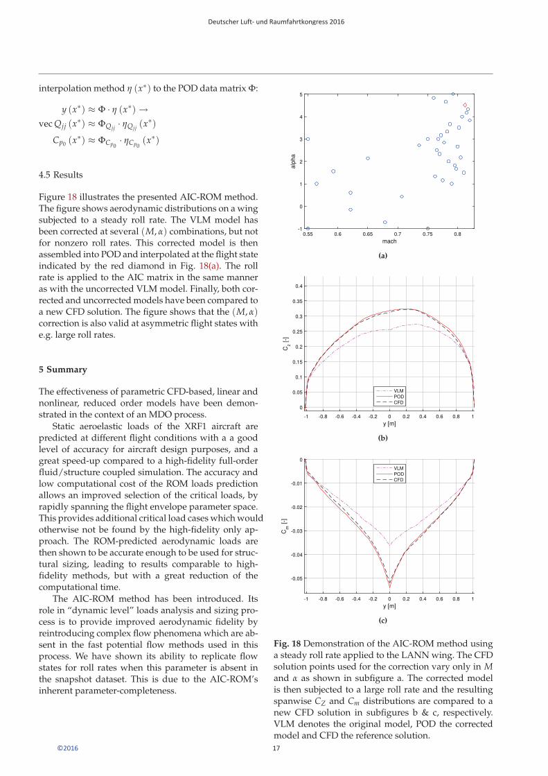
Figure 18 illustrates the presented AIC-ROM method.The figure shows aerodynamic distributions on a wingsubjected to a steady roll rate. The VLM model hasbeen corrected at several (M, α) combinations, but notfor nonzero roll rates. This corrected model is thenassembled into POD and interpolated at the flight stateindicated by the red diamond in Fig. 18(a). The rollrate is applied to the AIC matrix in the same manneras with the uncorrected VLM model. Finally, both cor-rected and uncorrected models have been compared toa new CFD solution. The figure shows that the (M, α)correction is also valid at asymmetric flight states withe.g. large roll rates.

5 Summary

The effectiveness of parametric CFD-based, linear andnonlinear, reduced order models have been demon-strated in the context of an MDO process.

Static aeroelastic loads of the XRF1 aircraft arepredicted at different flight conditions with a a goodlevel of accuracy for aircraft design purposes, and agreat speed-up compared to a high-fidelity full-orderfluid/structure coupled simulation. The accuracy andlow computational cost of the ROM loads predictionallows an improved selection of the critical loads, byrapidly spanning the flight envelope parameter space.This provides additional critical load cases which wouldotherwise not be found by the high-fidelity only ap-proach. The ROM-predicted aerodynamic loads arethen shown to be accurate enough to be used for struc-tural sizing, leading to results comparable to high-fidelity methods, but with a great reduction of thecomputational time.

The AIC-ROM method has been introduced. Itsrole in “dynamic level” loads analysis and sizing pro-cess is to provide improved aerodynamic fidelity byreintroducing complex flow phenomena which are ab-sent in the fast potential flow methods used in thisprocess. We have shown its ability to replicate flowstates for roll rates when this parameter is absent inthe snapshot dataset. This is due to the AIC-ROM’sinherent parameter-completeness.

mach0.55 0.6 0.65 0.7 0.75 0.8

alph

a

-1

0

1

2

3

4

5

(a)

y [m]-1 -0.8 -0.6 -0.4 -0.2 0 0.2 0.4 0.6 0.8 1

Cz

[-]

0

0.05

0.1

0.15

0.2

0.25

0.3

0.35

0.4

VLMPODCFD

(b)

y [m]-1 -0.8 -0.6 -0.4 -0.2 0 0.2 0.4 0.6 0.8 1

Cm

[-]

-0.05

-0.04

-0.03

-0.02

-0.01

0VLMPODCFD

(c)

Fig. 18 Demonstration of the AIC-ROM method usinga steady roll rate applied to the LANN wing. The CFDsolution points used for the correction vary only in Mand α as shown in subfigure a. The corrected modelis then subjected to a large roll rate and the resultingspanwise CZ and Cm distributions are compared to anew CFD solution in subfigures b & c, respectively.VLM denotes the original model, POD the correctedmodel and CFD the reference solution.


17©2016

References

1. Allmaras, S.R., Johnson, F.T.: Modifications andclarifications for the implementation of the spalart-allmaras turbulence model. In: Seventh Inter-national Conference on Computational Fluid Dy-namics (ICCFD7), pp. 1–11 (2012)

2. Astrid, P.: Reduction of process simulation mod-els: a proper orthogonal decomposition approach.Ph.D. thesis, Technische Universiteit Eindhoven(2004)

3. Astrid, P., Weiland, S., Willcox, K., Backx, T.:Missing point estimation in models described byproper orthogonal decomposition. AutomaticControl, IEEE Transactions on 53(10), 2237–2251(2008)

4. Barber, C.B., Dobkin, D.P., Huhdanpaa, H.: Thequickhull algorithm for convex hulls. ACM Trans-actions on Mathematical Software (TOMS) 22(4),469–483 (1996)

5. Barrault, M., Maday, Y., Nguyen, N.C., Patera,A.T.: An ‘empirical interpolation’method: appli-cation to efficient reduced-basis discretization ofpartial differential equations. Comptes RendusMathematique 339(9), 667–672 (2004)

6. Beckert, A., Wendland, H.: Multivariate interpo-lation for fluid-structure-interaction problems us-ing radial basis functions. Aerospace Science andTechnology 5(2), 125–134 (2001). DOI 10.1016/S1270-9638(00)01087-7

7. Bernstein, A.V., Kuleshov, A.P.: Tangent bundlemanifold learning via grassmann & stiefel eigen-maps. CoRR abs/1212.6031 (2012)

8. Brink-Spalink, J., Bruns, J.M.: Correction of Un-steady Aerodynamic Influence Coefficients usingExperimental or CFD Data. In: International Fo-rum on Aeroelasticity and Structural Dynamics(2001)

9. Bui-Thanh, T., Damodaran, M., Willcox, K.: Properorthogonal decomposition extensions for paramet-ric applications in transonic aerodynamics. In: Pro-ceedings of the 21th AIAA Applied AerodynamicsConference. AIAA, Orlando, Florida (2003). DOI10.2514/6.2003-4213

10. Cayton, L.: Algorithms for manifold learning.Univ. of California at San Diego Tech. Rep pp. 1–17(2005)

11. Chaturantabut, S., Sorensen, D.C.: Nonlinearmodel reduction via discrete empirical interpola-tion. SIAM Journal on Scientific Computing 32(5),2737–2764 (2010)

12. Forrester, A., Sobester, A., Keane, A.: Engineeringdesign via surrogate modelling: a practical guide.

John Wiley & Sons (2008)13. Fossati, M.: Evaluation of Aerodynamic Loads

via Reduced-Order Methodology. AIAA Journal(2015)

14. Fossati, M., Habashi, W.G.: Multiparameter anal-ysis of aero-icing problems using proper orthogo-nal decomposition and multidimensional interpo-lation. AIAA journal 51(4), 946–960 (2013)

15. Franz, T.: Reduced-order modeling for steady tran-sonic flows via manifold learning. Ph.D. thesis,TU Braunschweig (2016). URL http://www.digibib.tu-bs.de/?docid=00062584

16. Franz, T., Zimmermann, R., Gortz, S., Karcher, N.:Interpolation-based reduced-order modelling forsteady transonic flows via manifold learning. In-ternational Journal of Computational Fluid Dy-namics 28(3–4), 106–121 (2014)

17. Giesing, J.P., Kalman, T.P., Rodden, W.P.: Correc-tion Factor Techniques for Improving Aerody-namic Prediction Methods. Tech. rep., NASA(1976)

18. Gortz, S., Ilic, v., Liepelt, R.: Collaborative Multi-level MDO Process Development and Applicationto Long-ranged Transport Aircraft. In: ICAS (2016)

19. Hofstee, J., Kier, T., Cerulli, C., Looye, G.: A Vari-able, Fully Flexible Dynamic Response Tool forSpecial Investigations (VarLoads). In: Proceed-ings of the International Forum on Aeroelastic-ity and Structural Dynamics (IFASD). Amsterdam,The Netherlands (2003)

20. Holmes, P., Lumley, J.L., Gahl Berkooz, Rowley,C.W.: Turbulence, Coherent Structures, DynamicalSystems and Symmetry, first edn. Cambridge Uni-versity Press (1996). ISBN 978-0-521-55142-7

21. Jadic, I., Hartley, D., Giri, J.: An Enhanced Correc-tion Factor Technique for Aerodynamic InfluenceCoefficient Methods. In: MSC Aerospace User’sConference (1999)

22. Kroll, N., Abu-Zurayk, M., Dimitrov, D., Franz, T.,Fuhrer, T., Gerhold, T., Gortz, S., Heinrich, R., Ilic,C., Jepsen, J., Jagerskupper, J., Kruse, M., Krum-bein, A., Langer, S., Liu, D., Liepelt, R., Reimer,L., Ritter, M., Schwoppe, A., Scherer, J., Spiering,F., Thormann, R., Togiti, V., Vollmer, D., Wendisch,J.H.: Dlr project digital-x: Towards virtual aircraftdesign and flight testing based on high-fidelitymethods. CEAS Aeronautical Journal 7(1), 3–27(2016)

23. Langer, S., Schwoppe, A., Kroll, N.: The DLR flowsolver TAU-status and recent algorithmic develop-ments. In: 52nd AIAA Aerospace Sciences Meet-ing. AIAA Paper, vol. 80 (2014)


18©2016

24. LeGresley, P.A., Alonso, J.J.: Investigation of Non-Linear Projection for POD Based Reduced OrderModels for Aerodynamics. In: Proceedings of the39th AIAA Aerospace Sciences Meeting and Ex-hibit, vol. 926, p. 2001. Reno, Nevada (2001)

25. Leitner, M., Liepelt, R., Kier, T., Klimmek, T.,Muller, R., Schulze, M.: A Fully Automatic Struc-tural Optimization Framework to Determine Crit-ical Design Loads. In: Deutscher Luft- undRaumfahrt Kongress 2016. Braunschweig, Ger-many (2016)

26. Lucia, D.J., Beran, P.S., Silva, W.A.: Reduced-order modeling: new approaches for computa-tional physics. Progress in Aerospace Sciences40(1), 51–117 (2004)

27. Van der Maaten, L., Postma, E., Van den Herik, H.:Dimensionality reduction: A comparative review.Journal of Machine Learning Research 10, 1–41(2009)

28. Mardia, K., Kent, J., Bibby, J.: Multivariate analysis.Academic press (1979)

29. More, J.J.: The levenberg-marquardt algorithm:implementation and theory. In: Numerical anal-ysis, pp. 105–116. Springer (1978)

30. Narayanan, H., Mitter, S.: Sample complexity oftesting the manifold hypothesis. In: Advances inNeural Information Processing Systems, pp. 1786–1794 (2010)

31. Penrose, R.: On best approximate solutions of lin-ear matrix equations. Mathematical Proceedingsof the Cambridge Philosophical Society 52(1), 17–19 (1956)

32. Piperni, P., DeBlois, A., Henderson, R.: De-velopment of a multilevel multidisciplinary-optimization capability for an industrial environ-ment. AIAA Journal 51, 2335–2352 (2013). DOI10.2514/1.J052180

33. Rajan, V.: Optimality of the delaunay triangulationin Rd. Discrete & Computational Geometry 12(1),189–202 (1994)

34. Schilders, W.H., Van Der Vorst, H.A., Rommes,J.: Model order reduction: theory, research aspectsand applications, vol. 13. Springer (2008)

35. Schwamborn, D., Gerhold, T., Heinrich, R.: TheDLR TAU-code: recent applications in researchand industry, tech. report. In: European Confer-ence on Computational Fluid Dynamics, ECCO-MAS CFD 2006. Egmond and Zee, The Nether-lands (2006)

36. Shlens, J.: A tutorial on principal component anal-ysis. Systems Neurobiology Laboratory, Univer-sity of California at San Diego (2005)

37. Tenenbaum, J.B., de Silva, V., Langford, J.C.: AGlobal Geometric Framework for Nonlinear Di-mensionality Reduction. Science 290(5500), 2319–2323 (2000)

38. Tropea, C., Yarin, A., Foss, J.: Springer Handbookof Experimental Fluid Mechanics. Springer-VerlagBerlin Heidelberg (2007)

39. Vendl, A., Faßbender, H.: Model order reductionfor unsteady aerodynamic applications. In: Proc.Appl. Math. Mech., vol. 13, pp. 475–476 (2013)

40. Vendl, A., Faßbender, H., Gortz, S., Zimmermann,R., Mifsud, M.: Model order reduction for steadyaerodynamics of high-lift configurations. CEASAeronautical Journal 5(4), 487–500 (2014)

41. Wild, J.: Aeroforce - thrust/drag bookkeeping andaerodynamic force breakdown over components.Tech. rep., German Aerospace Center (DLR) (1999)

42. Wright, S., Nocedal, J.: Numerical optimization,vol. 2. Springer New York (1999)

43. Zill, T., Bohnke, D., Nagel, B.: Preliminary AircraftDesign in a Collaborative Multidisciplinary De-sign Environment. In: AIAA Aviation Technology,Integration and Operations (2011)

44. Zimmermann, R., Gortz, S.: Non linear reducedorder models for steady aerodynamics. In: Proce-dia Computer Science, vol. 1, pp. 165–174 (2010).Proceedings of the International Conference onComputational Science, ICCS 2010

45. Zimmermann, R., Gortz, S.: Improved extrapo-lation of steady turbulent aerodynamics using anon-linear POD-based reduced order model. TheAeronautical Journal 116(1184), 1079–1100 (2012)

46. Zimmermann, R., Vendl, A., Gortz, S.: Reduced-order modeling of steady flows subject to aerody-namic constraints. AIAA Journal pp. 1–12 (2014)

47. Zimmermann, R., Willcox, K.: An acceleratedgreedy missing point estimation procedure. SIAMJournal on Scientific Computing (2016). Acceptedfor publication


19©2016

Documents

Reduced Order Models for Aerodynamic Applications, Loads