REDUCED-COMPLEXITY EPILEPTIC SEIZURE PREDICTION WITH EEG

A DISSERTATION

SUBMITTED TO THE FACULTY OF THE GRADUATE SCHOOL

OF THE UNIVERSITY OF MINNESOTA

BY

Yun Sang Park

IN PARTIAL FULFILLMENT OF THE REQUIREMENTS

FOR THE DEGREE OF

DOCTOR OF PHILOSOPHY

Professor Keshab K. Parhi, Advisor; Professor Theoden I. Netoff, Co-advisor

January 2012

© Yun Sang Park 2012

i

Acknowledgements

First of all, I wish to thank my advisor, Professor Keshab K. Parhi, and my co-advisor,

Professor Theoden I. Netoff, for their continuing encouragement, guidance, and financial

support throughout my Ph.D. study at the University of Minnesota. Especially, I am

grateful that I have had research opportunities in the interdisciplinary area of brain signal

processing using machine learning techniques.

I would like to thank Professor Mostafa Kaveh and Professor Emad Ebbini for their

support as members of my Ph.D. committee. I would also like to thank Professor

Vladimir S. Cherkassky and Dr. Timothy Denison for their helpful comments and

suggestions. Especially, I would like to thank Dr. Xiaofeng Yang for providing me with

his datasets and helping me understand his seizure detection system.

I would like to thank the Graduate School and the Institute of Engineering and

Medicine of the University of Minnesota for their financial support with the

Interdisciplinary Doctoral Fellowship award and a research grant. I would also like to

thank the Freiburg EEG Database at the University of Freiburg for providing the

numerous EEG datasets of epileptics. I would like to thank the Minnesota

Supercomputing Institute at the University of Minnesota for supporting the computational

power and providing the technical assistance as well.

My thanks also go to current and former members of our research group. Particularly,

Lan Luo and Manohar Ayinala for our numerous discussions on a variety of research

topics. Also, I am grateful to Chuan Zhang and Sohini Roy Chowdhury for their support

and engagement in my Ph.D.

I would like to also thank my friends at the University and in my country South Korea,

especially Cheol-hong Min, Hyun-Chul Jang, Hanyong Eom, Won-Cheol Yoo, In-Young

Hur, and Kyung-Seok Seoh, for their assistance and engagement to continue my studies.

Lastly, I am forever grateful to my parents, my sister and brother, and especially my

lovely wife, who has missed me in South Korea while having our unborn baby in her, for

their love, support, and encouragement throughout the years. Without them, I could not

have completed my Ph.D. successfully.

ii

Abstract

In the dissertation we seek to develop and validate reliable frameworks for human

epileptic seizure prediction with electrocorticogram (ECoG) and intracranial

electroencephalogram (iEEG). The long-term goal of the research is to develop and

prototype an implantable device that can reliably provide alarms prior to a seizure in real-

time. The specific objective is to develop a patient-specific algorithm that can predict

seizures in ECoG/iEEG with high sensitivity and low false positive rate as well as low

complexity. This dissertation starts by demonstrating that seizures can be predicted with

linear features of spectral power, and it ultimately focuses on developing a reduced-

complexity algorithm that can decode ECoG/iEEG for human epileptic seizure prediction

with high sensitivity and acceptable low false positive rate. By contrast to prior

prediction work, most of which focused on nonlinear measurements, we demonstrate that

human epileptic seizures can be predicted with linear features of ECoG/iEEG in machine

learning classification approach.

To begin with, a new patient-specific seizure prediction algorithm with

ECoG/iEEG is proposed. It is novel in sense that it employs a set of linear features of

spectral power from ECoG/iEEG for prediction and that predictive models are

established and tested using cost-sensitive support vector machines (SVMs) using double

cross-validation method. The proposed algorithm is tested over 433.2 hours of interictal

recordings including 80 seizure events from 18 human epileptics in the Freiburg EEG

database. It achieves high sensitivity of 97.5% (78/80), a low false alarm rate of 0.27 per

iii

hour (total 117 FPs), and total false prediction times of 13.0% (56.4-hour). Bipolar

and/or time-differential preprocessing improves sensitivity and false positive rate.

For the seizure prediction algorithm to be practically feasible on an implantable

device, we further propose a reduced-complexity prediction algorithm. We lower the

complexity of the algorithm by investigating and using small numbers of essential

features and by replacing nonlinear SVMs and the Kalman filter with linear SVMs and

moving-average filters. The key features are determined using the RFE SVM (recursive

feature elimination using SVMs). The proposed reduced-complexity algorithm

significantly lowers the predictor’s complexity and thus the power consumption, while

producing high sensitivity as well as reasonable false positives. It is tested on 9 subjects

selected from the Freiburg database that result in high prediction rate when the initial

prediction algorithm is applied, and successfully demonstrates high sensitivity of 100.0%

(38/38) as well as low false positive rate of 0.15 per hour (total 32 FPs) and false positive

portion of 9.65% (21.0-hour) in the 217.5-hour interictal recordings with the selected six

time-differential features. It has been observed that time-differential preprocessing

improves the prediction rate significantly.

Additionally, we develop an enhanced approach for seizure onset and offset

detection in rats’ ECoG. This is an improved version of the automatic seizure detection

and termination system in in-vivo rats’ ECoG. We improve the system by using a

specific frequency range of 14-22Hz, which has been observed to be more relevant to

seizure onsets than other bands; by using spectral power instead of spectral amplitudes as

a feature set; and by substituting the 2-point moving average filter with the Kalman filter.

iv

Furthermore, while the proposed algorithm provides better detection statistics, it also

lowers the system’s complexity by removing the fast Fourier transform computation and

keeping a single structure though the proposed algorithm uses the two different spectral

features for detecting onsets and offsets.

v

Table of Contents

Acknowledgements…………………………….………………………………………...………………i

Abstract……………………………………………………………………...……………………..............ii

List of Tables……………………………………………………………………...……………………...xi

List of Figures……………………………………………………………………...……………………xii

..................................................................................................... 1 Chapter 1 Introduction

Introduction ........................................................................................................... 1 1. 1

Summary of Contributions .................................................................................... 4 1. 2

Seizure Prediction with Spectral Power of iEEG Using SVMs ..................... 4 1. 2. 1

Reduced Complexity of Seizure Prediction with iEEG ................................. 6 1. 2. 2

Enhanced Seizure Detection in Rats’ ECoG .................................................. 7 1. 2. 3

Outline of the Thesis ............................................................................................. 9 1. 3

................................................................................................... 11 Chapter 2 Background

Introduction to Epilepsy and Seizure Prediction ................................................. 11 2. 1

Prior Work in Seizure Prediction with EEG ....................................................... 15 2. 2

Early-Phase Attempts with Linear Measures ............................................... 16 2. 2. 1

Promising Nonlinear Analysis ..................................................................... 16 2. 2. 2

Skepticism on Nonlinear Measures ............................................................. 17 2. 2. 3

Main Barriers to Progress in Seizure Prediction Research .......................... 17 2. 2. 4

vi

Recent Research Trend in Seizure Prediction and Detection with EEG ............. 18 2. 3

Machine Learning Approaches .................................................................... 18 2. 3. 1

Commercial Efforts ...................................................................................... 20 2. 3. 2

Technical Backgrounds ....................................................................................... 21 2. 4

Moving Window Analysis ........................................................................... 21 2. 4. 1

Support Vector Machine Classification ....................................................... 21 2. 4. 2

Cross-Validation .......................................................................................... 24 2. 4. 3

Kalman Filter ............................................................................................... 24 2. 4. 4

Sensitivity, Specificity, False Positive Rate per Hour, and False Positive 2. 4. 5

Percentage .................................................................................................... 27

Fβ-measure ................................................................................................... 28 2. 4. 6

p-value.......................................................................................................... 29 2. 4. 7

Receiver Operating Characteristic Analysis ................................................ 30 2. 4. 8

.................... 32 Chapter 3 Seizure Prediction with Spectral Power of iEEG Using SVMs

Introduction ......................................................................................................... 32 3. 1

Methods ............................................................................................................... 35 3. 2

Outline.......................................................................................................... 35 3. 2. 1

Dataset Description ...................................................................................... 36 3. 2. 2

Preprocessing: Removing Artifacts of iEEG Recordings ............................ 36 3. 2. 3

vii

Feature Extraction ........................................................................................ 38 3. 2. 4

SVM Classification Using Double Cross-Validation .................................. 41 3. 2. 5

Postprocessing: Suppressing Isolated False Positives ................................. 45 3. 2. 6

Kernel Fisher Discriminant Analysis ........................................................... 47 3. 2. 7

Results ................................................................................................................. 48 3. 3

Discussions .......................................................................................................... 56 3. 4

Conclusion ........................................................................................................... 63 3. 5

..................................... 64 Chapter 4 Reduced-Complexity Seizure Prediction with EEG

Introduction ......................................................................................................... 64 4. 1

Methods ............................................................................................................... 65 4. 2

Overview ...................................................................................................... 65 4. 2. 1

Dataset Description ...................................................................................... 67 4. 2. 2

Recursive Feature Elimination Using SVMs ............................................... 67 4. 2. 3

Feature Selection by RFE SVM for Reduced Complexity Seizure Prediction4. 2. 4

...................................................................................................................... 69

Postprocessing by Kalman Filter or Moving-Average Filter ....................... 75 4. 2. 5

Results ................................................................................................................. 76 4. 3

RFE SVM Results ........................................................................................ 76 4. 3. 1

Discussions .......................................................................................................... 88 4. 4

viii

Conclusion ........................................................................................................... 92 4. 5

................................. 93 Chapter 5 Enhanced Seizure Detection System with Rats' ECoG

Introduction ......................................................................................................... 93 5. 1

Methods ............................................................................................................... 94 5. 2

Dataset Description ...................................................................................... 94 5. 2. 1

Prior Seizure Onset and Offset Detection Approach ................................... 97 5. 2. 2

Time-Frequency Analysis on Onsets ........................................................... 98 5. 2. 3

Time-Frequency Analysis on Offsets .......................................................... 98 5. 2. 4

Proposed Seizure Onset and Offset Detection Approach .......................... 101 5. 2. 5

Results ............................................................................................................... 102 5. 3

Prior Approach for Onset Detection Using Spectral Amplitudes in 5-35Hz 5. 3. 1

and 2-point Moving-Average Fitler ........................................................... 103

Proposed Approach for Onset Detection Using Spectral Power in 14-22Hz 5. 3. 2

and the Kalman Filter................................................................................. 107

Approach for Onset Detection Using Line-Length .................................... 108 5. 3. 3

Result Comparison for Onset Detection .................................................... 108 5. 3. 4

Proposed Approach for Offset Detection Using Spectral Power in 7-45Hz 5. 3. 5

and the Kalman Filter................................................................................. 109

Testing Proposed Algorithm in Continuous Recording ............................. 110 5. 3. 6

ix

Discussions ........................................................................................................ 113 5. 4

Conclusion ......................................................................................................... 116 5. 5

.............................................. 117 Chapter 6 Conclusions and Future Research Directions

Conclusions ....................................................................................................... 117 6. 1

Seizure Prediction with Spectral Power of ECoG/iEEG using SVMs ...... 118 6. 1. 1

Reduced Complexity Seizure Prediction with Linear SVMs .................... 119 6. 1. 2

Enhanced Seizure Detection with Rat’s ECoG .......................................... 119 6. 1. 3

Future Research Directions ............................................................................... 120 6. 2

Extending and validating our prediction approach onto the larger database of 6. 2. 1

Mayo .......................................................................................................... 120

Improving the predictor by testing wavelet features and finding optimized 6. 2. 2

parameters in the algorithm ....................................................................... 121

Testing other classification methods and investigating key features using 6. 2. 3

other approaches ........................................................................................ 122

Implementing the proposed algorithm for enhanced seizure detection with 6. 2. 4

in-vivo rats’ ECoG in LabVIEW................................................................ 123

Investigating hardware architectures for a real-time seizure predictor and 6. 2. 5

developing it in hardware ........................................................................... 123

Extending the machine-learning-based classification to other neuronal 6. 2. 6

applications ................................................................................................ 124

x

Bibliography ................................................................................................................... 125

xi

List of Tables

Table 2.1 Confusion matrix ............................................................................................. 28

Table 3.1 Results from the proposed seizure prediction algorithm on the Freiburg

database ................................................................................................................. 51

Table 3.2 Results from different postprocessing methods in bipolar recordings ............ 52

Table 3.3 Top two discriminating raw or time-differential features ................................ 53

Table 3.4 Results from initial analysis with 5-min moving window and SVM

classification with polynomial kernel ................................................................... 54

Table 3.5 Results from the other initial analysis using SVM classification and k-of-n

analysis by double cross-validation ...................................................................... 55

Table 4.1 Summary results from the RFE SVM analysis for all the patients and all the

four preprocessing methods (KF applied as postprocessing) ............................... 78

Table 4.2 Top features selected in RFE SVM analysis in Patient 6 ................................ 78

Table 4.3 Postprocessing effects: results with 6 and 9 time-differential features by

different methods of postprocessing ..................................................................... 82

Table 4.4 Seizure prediction results with 6 time-differential iEEG using linear SVMs and

20-tap moving-average filter ................................................................................. 83

Table 4.5 Seizure prediction results with 9 time-differential iEEG using linear SVMs and

20-tap moving-average filter ................................................................................. 84

Table 5.1 Onset detection result summary and comparison ........................................... 109

xii

List of Figures

Figure 2.1 Open-loop and close-loop systems for seizure intervention ........................... 13

Figure 2.2 Bulky pacemaker in 1940s (left) and modern pacemaker (right) ................... 14

Figure 2.3 Commercial products for anti-seizure systems ............................................... 20

Figure 2.4 Moving window analysis with half-overlapped windows .............................. 21

Figure 2.5 Support Vector Machine Classification [14] .................................................. 22

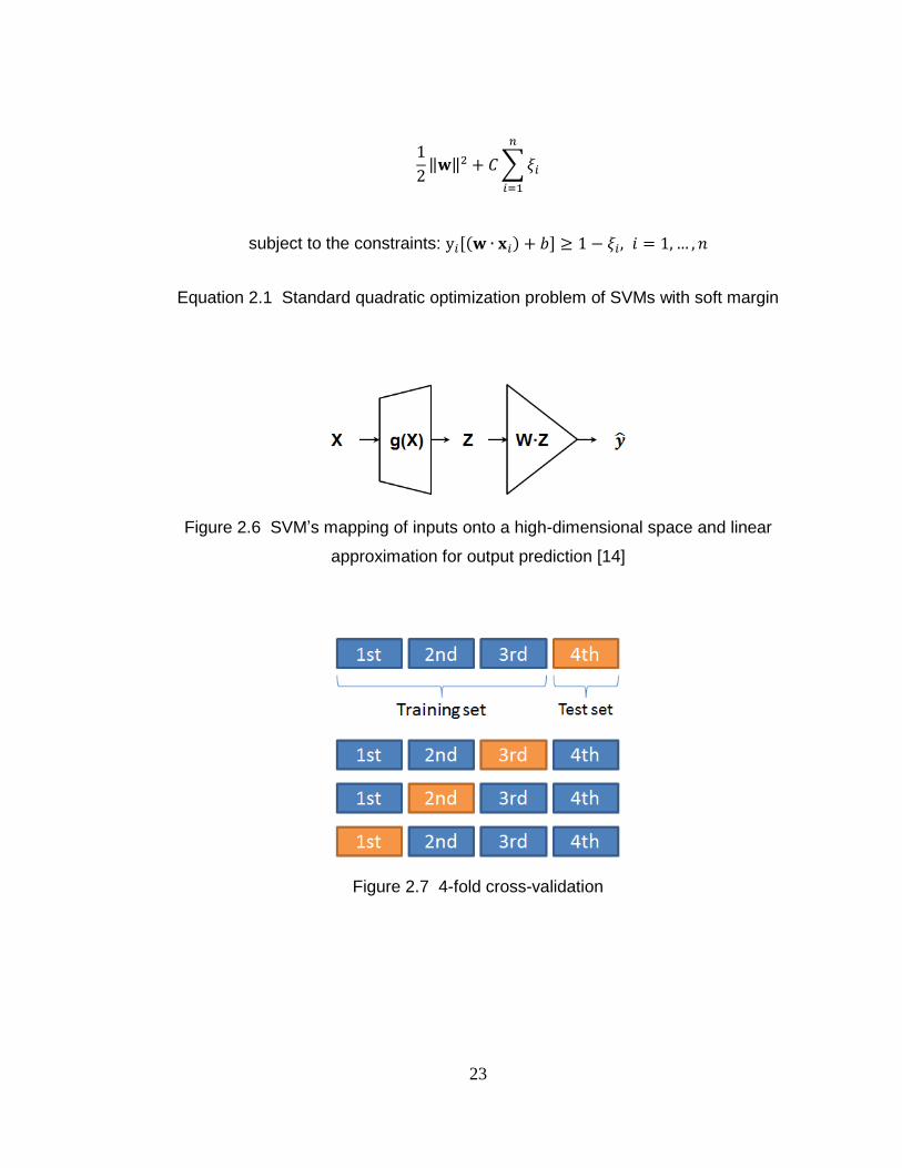
Figure 2.6 SVM’s mapping of inputs onto a high-dimensional space and linear

approximation for output prediction [14] ............................................................. 23

Figure 2.7 4-fold cross-validation .................................................................................... 23

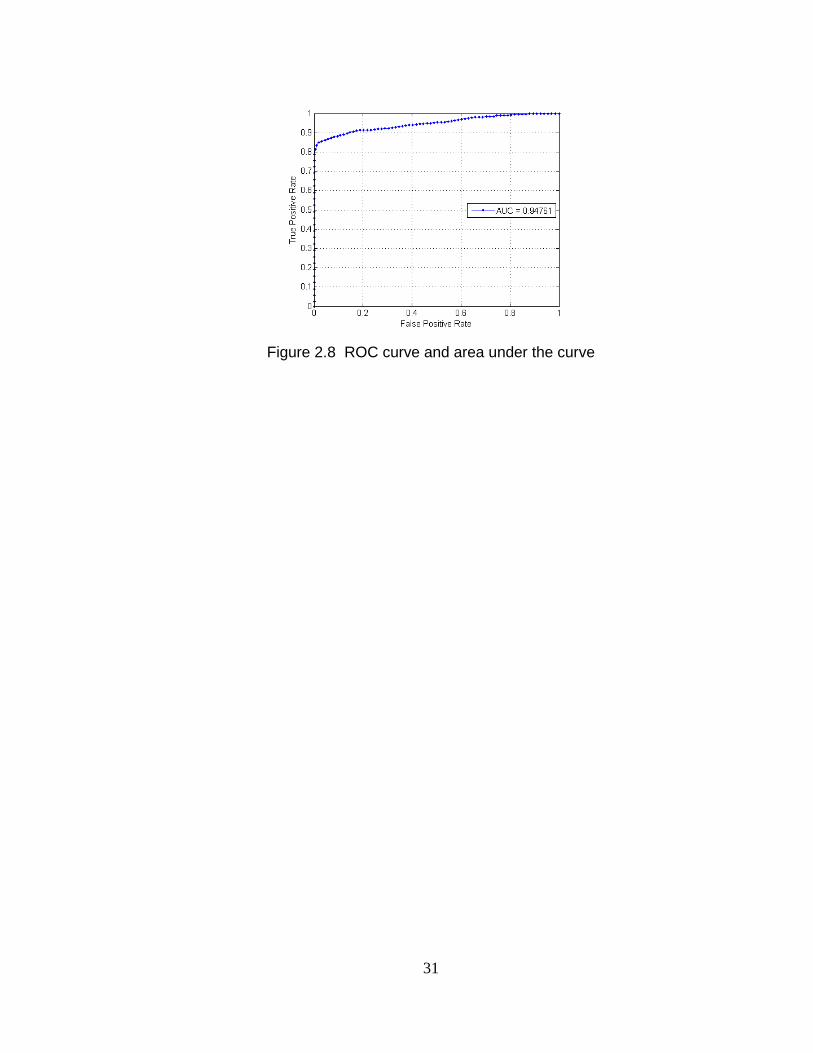
Figure 2.8 ROC curve and area under the curve .............................................................. 31

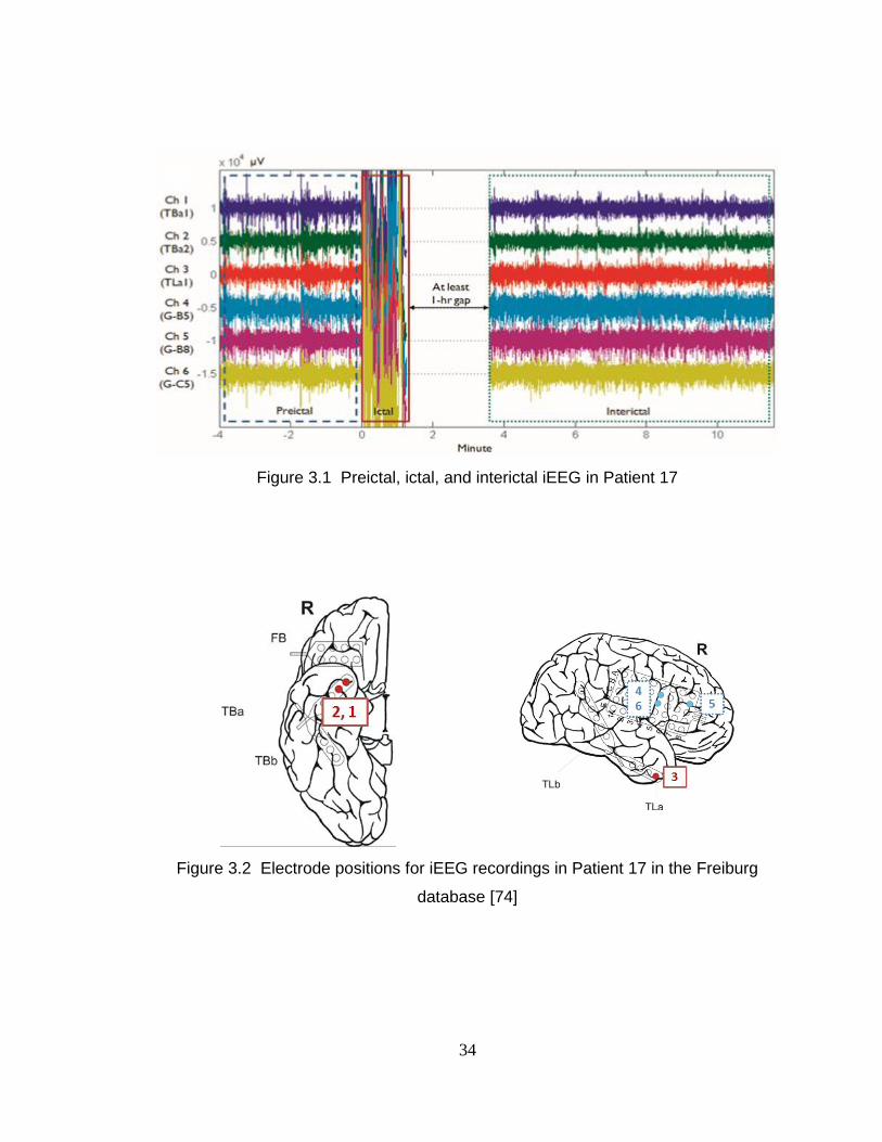
Figure 3.1 Preictal, ictal, and interictal iEEG in Patient 17 ............................................. 34

Figure 3.2 Electrode positions for iEEG recordings in Patient 17 in the Freiburg database

[74] ........................................................................................................................ 34

Figure 3.3 Outline of the proposed seizure prediction algorithm .................................... 35

Figure 3.4 Preictal iEEG (left column), interictal iEEG (middle), and their power spectral

density (right) in the four different preprocessing methods.................................. 40

Figure 3.5 Effects of increases in cost-sensitive parameter R in SVM classification. The

blue points represent interictal samples and red ones preictal. The two principal

components of each of preictal and interictal are used in the figures. The points in

the green area are the ones predicted as preictal by the SVM. ............................. 42

xiii

Figure 3.6 Grid search with log2Cost and log2Ratio ........................................................ 43

Figure 3.7 Examples of SVM classification and Kalman filter postprocessing in testing

data (a) with ictal recordings and (b) with interictal recordings ........................... 46

Figure 3.8 4-of-7 analysis ................................................................................................ 47

Figure 3.9 Histograms of decision function values produced by the linear SVM in (a)

training and (b) testing sets ................................................................................... 58

Figure 3.10 High-pass filtered preictal iEEG recordings (>30Hz, top) and its original

signal’s spectrogram (bottom) .............................................................................. 59

Figure 3.11 Typical results from SVM classification and postprocessing by the Kalman

filter in ictal recordings. In most cases, seizures are “anticipated”: our algorithm

could not distinguish 30-min preictal iEEG and iEEG preceding it. .................... 60

Figure 4.1 Outline of the proposed reduced complexity seizure prediction algorithm ... 66

Figure 4.2 Backward feature elimination......................................................................... 66

Figure 4.3 Electrode positions in Patient 6 in the Freiburg database............................... 72

Figure 4.4 Preictal iEEG (left column) and interictal iEEG (middle column) and their

power spectral density (right column) in Patient 6 in all the four preprocessing

methods: (a) raw, (b) time-differential, (c) bipolar, and (d) bipolar/time-

differential ............................................................................................................. 74

Figure 4.5 Results from two-step RFE SVM analyses with all the four sets of

preprocessed features. ........................................................................................... 77

xiv

Figure 4.6 Classification rates with certain numbers of selected features for all the four

preprocessed methods (KF applied) ...................................................................... 81

Figure 4.7 Graphical comparison in classification results by postprocessing method .... 86

Figure 4.8 Final output comparison between the proposed linear approach with six top

features and the reference [5] ................................................................................ 87

Figure 5.1 Spargue-Dawley rat with ECoG electrodes (left) and ECoG electrode

placement (right) [16]. The red-circled electrode is the one where the mainly

analyzed ECoG in the chapter was recorded. ....................................................... 95

Figure 5.2 LabVIEW front panel for seizure detection system ....................................... 96

Figure 5.3 Outline for prior seizure detection system....................................................... 96

Figure 5.4 ECoG recordings (top pictures of each) and their spectrograms (bottom

pictures of each) on various seizure onsets ........................................................... 99

Figure 5.5 ECoG recordings (top pictures of each) and their spectrograms (bottom

pictures of each) on various seizure offsets ........................................................ 100

Figure 5.6 Proposed algorithm for seizure onset and offset detection ........................... 101

Figure 5.7 Prior algorithm’s features (spectral amplitudes in 5-35Hz and their 2-pt MA-

filtered values) on seizure onsets ........................................................................ 104

Figure 5.8 ROC analysis in 2-pt MA-filtered spectral amplitudes in 5-35Hz ............... 104

Figure 5.9 Proposed algorithm’s features (spectral power in 14-22Hz and its Kalman-

filtered values) on seizure onsets ........................................................................ 105

xv

Figure 5.10 ROC analysis in Kalman-filtered spectral power in 14-22Hz .................... 105

Figure 5.11 Kalman-filtered line-length features on seizure onsets .............................. 106

Figure 5.12 ROC analysis in Kalman-filtered line-length ............................................. 106

Figure 5.13 ECoG signals (top in left), their spectrogram (middle), and the corresponding

offset features (bottom) on offsets. The right figures are enlarged ones of the

offset features that are placed in left bottom. ...................................................... 111

Figure 5.14 Seizure onset and offset detection in continuous recording ....................... 112

Figure 5.15 Comparison between features on an onset ................................................. 115

1

Chapter 1

Introduction

Introduction 1. 1

Epilepsy is the second most common neurological disorder after stroke [1]. One in ten

adults will experience a seizure at some point in their life, and approximately one in

hundred people will experience multiple seizures, classifying them as epileptics. It is

estimated that up to 1% of the world’s population suffer from epilepsy and nearly three

million people in the U.S. are affected by the disease [1-3]. In the U.S., it costs over 15

billion dollars directly and indirectly due to the disease.

Anti-epileptic drugs are the most common therapy against epilepsy. Anti-

convulsant medication eliminates all seizures for over half of chronic epileptics and at

least reduces the number of seizures for an additional 20 to 30 percent. Resective brain

surgery, which excises the seizure foci, is the therapy used in drug-resistant patients.

However, both methods have the serious disadvantages. First, the anti-convulsant

2

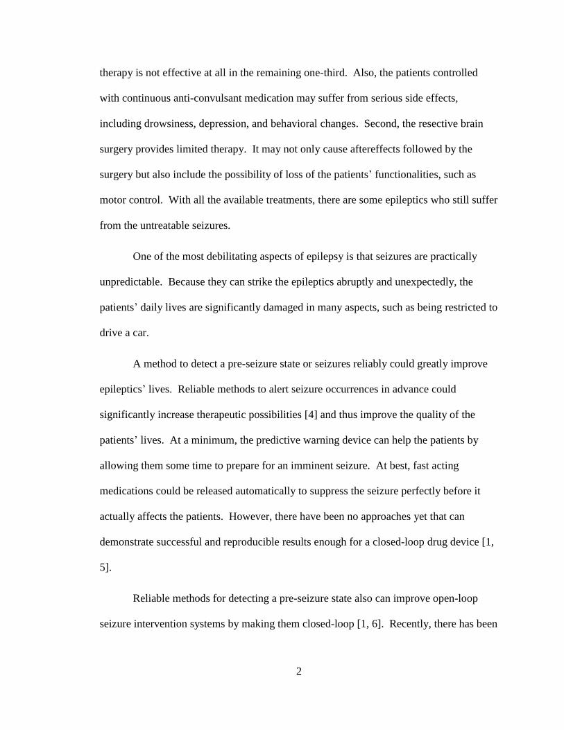
therapy is not effective at all in the remaining one-third. Also, the patients controlled

with continuous anti-convulsant medication may suffer from serious side effects,

including drowsiness, depression, and behavioral changes. Second, the resective brain

surgery provides limited therapy. It may not only cause aftereffects followed by the

surgery but also include the possibility of loss of the patients’ functionalities, such as

motor control. With all the available treatments, there are some epileptics who still suffer

from the untreatable seizures.

One of the most debilitating aspects of epilepsy is that seizures are practically

unpredictable. Because they can strike the epileptics abruptly and unexpectedly, the

patients’ daily lives are significantly damaged in many aspects, such as being restricted to

drive a car.

A method to detect a pre-seizure state or seizures reliably could greatly improve

epileptics’ lives. Reliable methods to alert seizure occurrences in advance could

significantly increase therapeutic possibilities [4] and thus improve the quality of the

patients’ lives. At a minimum, the predictive warning device can help the patients by

allowing them some time to prepare for an imminent seizure. At best, fast acting

medications could be released automatically to suppress the seizure perfectly before it

actually affects the patients. However, there have been no approaches yet that can

demonstrate successful and reproducible results enough for a closed-loop drug device [1,

5].

Reliable methods for detecting a pre-seizure state also can improve open-loop

seizure intervention systems by making them closed-loop [1, 6]. Recently, there has been

3

great progress in open-loop seizure intervention therapy, such as the Deep Brain

Stimulation Therapy [7], as well as in closed-loop therapy, such as the Responsive

Neuro-stimulation System [6]. The open-loop systems operate following a preset

schedule for stimulation. By contrast, a closed-loop seizure intervention system is

expected to alarm a seizure attack in advance, trigger rescue therapy, and suppress the

seizure occurrence. This closed-loop system could increase efficacy and lower the

possibility of side effects, compared with the open-loop ones [2, 8].

Our ultimate objective is to develop an implantable device that can reliably

provide an alert in advance to an impending seizure attack and further produce seizure

prediction time sufficient to prepare triggering anti-epileptic therapy. The specific

objective of the research is to develop and test reliable, cost-effective, and power-

efficient algorithms for seizure prediction. The central hypothesis is that seizures can be

predicted in the approach of the binary classification between pre-seizure states and

ordinary states of iEEG. Also, we hypothesize that through the use of the optimal sets of

linear features of iEEG and machine-learning-based classifiers, we will be able to a

design a reliable seizure prediction model.

This thesis is devoted to developing and testing an approach for reliable seizure

prediction using linear features of iEEG and a machine learning classifier, and further to

developing a reduced-complexity algorithm for seizure prediction. Our contributions are

listed in the next section as follows.

4

Summary of Contributions 1. 2

Seizure Prediction with Spectral Power of iEEG Using SVMs 1. 2. 1

We have proposed a patient-specific algorithm for seizure prediction using linear features

of spectral power from iEEG and a machine learning classifier of support vector

machines (SVMs) [5, 9, 10]. Using the proposed algorithm, we have demonstrated that

seizures can be predicted using linear features of spectral power of iEEG and nonlinear

SVM classification. Prior work on seizure prediction demonstrated that seizures may be

predicted using linear measures of spectral power from iEEG [1, 11, 12]. Compared to

the prior work, we have developed our seizure prediction approach by combining all

potential features of spectral power and classifying them in multivariate approach using

the machine learning technique of SVMs. Our proposed algorithm has achieved high

sensitivity of 97.5% with total 80 seizures and a low false alarm rate of 0.27 per hour in a

total of 433.2 interictal hours across 18 patients in the Freiburg database.

We have applied a statistical validation approach of double cross-validation [13,

14] in evaluation of seizure prediction algorithms. In many of prior seizure prediction

studies, algorithms were trained and tested on the same datasets, and this led to inflated

optimistic results that could be achieved only on their own datasets. By contrast, in the

double cross-validation approach, where a dataset is split into a training set and a test set

and the training set is further split into a learning set and a validation set, we have

achieved in-sample optimization and out-of-sample testing. We believe that double

cross-validation is a statistical methodology to estimate prediction rate that can be

5

expected in real-world conditions, especially when machine learning classification

approaches are used.

Bipolar and/or time-differential preprocessing methods have been tested in our

algorithm and those preprocessing methods have led to better prediction rate than raw

iEEG. Compared to seizure prediction with raw iEEG that results in sensitivity of 93.8%

and false positive rate of 0.29 per hour, prediction with bipolar iEEG results in higher

sensitivity of 97.5% as well as lower false positive rate of 0.27 per hour. Time-

differential preprocessing leads to further lower false positive rate of 0.20 per hour,

though it slightly decreases the sensitivity to 92.5%.

F2-measure, which will be explained in the next chapter, has been introduced to

seizure prediction work to evaluate the prediction rate as a single measure. In the prior

studies, sensitivity and specificity, or sensitivity, false positive rate per hour, and false

positive percent in interictal recordings were proposed for evaluating prediction

algorithms’ performance. However, they do not measure a single quantity. For the case

when estimated models are required to be evaluated and compared by a single criterion,

F2-measue can represent the prediction rate as a single statistic.

In addition, in the Kernel Fisher Discriminant analysis, we have found out that

high frequency components in iEEG may play a crucial role in seizure prediction.

Gamma frequency bands have turned out to be the most discriminating. In this sense, we

believe that the time-differential preprocessing may improve seizure prediction rate.

6

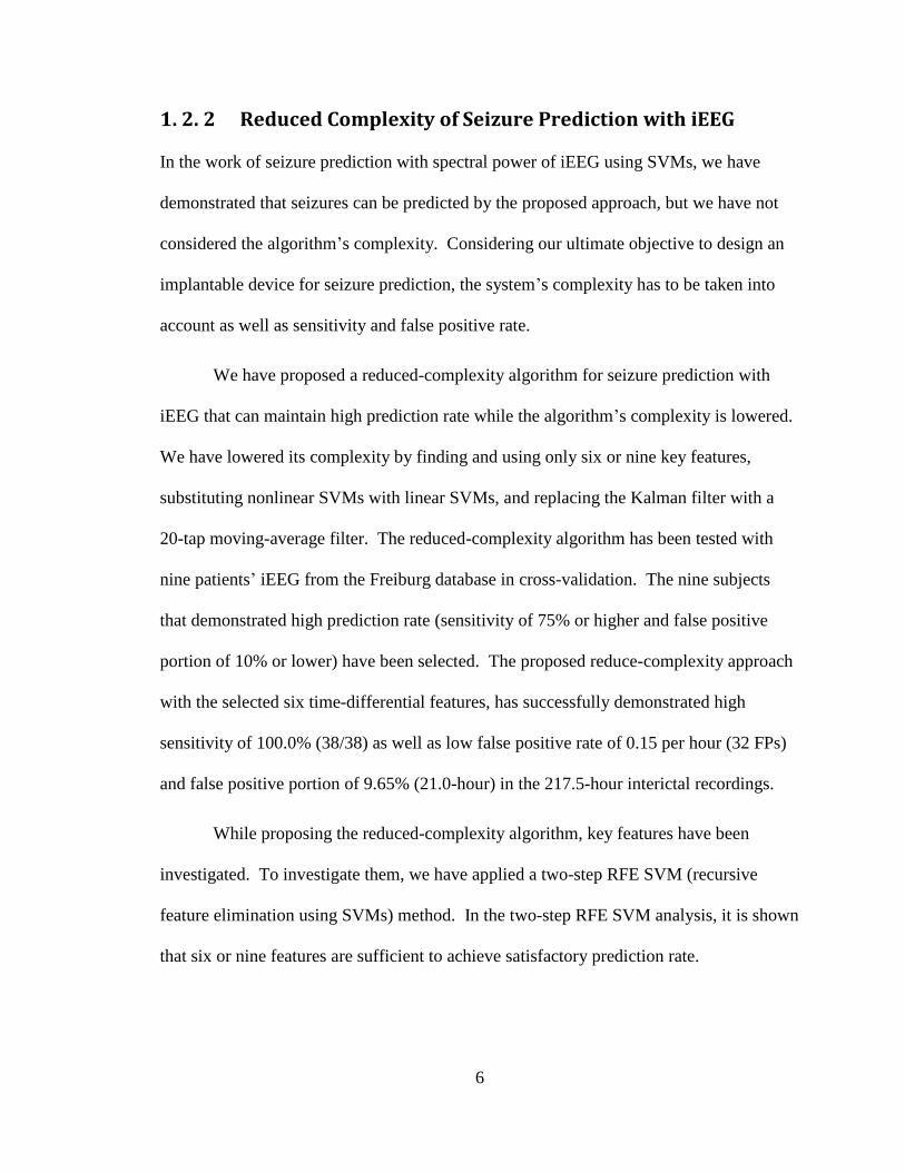
Reduced Complexity of Seizure Prediction with iEEG 1. 2. 2

In the work of seizure prediction with spectral power of iEEG using SVMs, we have

demonstrated that seizures can be predicted by the proposed approach, but we have not

considered the algorithm’s complexity. Considering our ultimate objective to design an

implantable device for seizure prediction, the system’s complexity has to be taken into

account as well as sensitivity and false positive rate.

We have proposed a reduced-complexity algorithm for seizure prediction with

iEEG that can maintain high prediction rate while the algorithm’s complexity is lowered.

We have lowered its complexity by finding and using only six or nine key features,

substituting nonlinear SVMs with linear SVMs, and replacing the Kalman filter with a

20-tap moving-average filter. The reduced-complexity algorithm has been tested with

nine patients’ iEEG from the Freiburg database in cross-validation. The nine subjects

that demonstrated high prediction rate (sensitivity of 75% or higher and false positive

portion of 10% or lower) have been selected. The proposed reduce-complexity approach

with the selected six time-differential features, has successfully demonstrated high

sensitivity of 100.0% (38/38) as well as low false positive rate of 0.15 per hour (32 FPs)

and false positive portion of 9.65% (21.0-hour) in the 217.5-hour interictal recordings.

While proposing the reduced-complexity algorithm, key features have been

investigated. To investigate them, we have applied a two-step RFE SVM (recursive

feature elimination using SVMs) method. In the two-step RFE SVM analysis, it is shown

that six or nine features are sufficient to achieve satisfactory prediction rate.

7

Another important aspect that we have observed is that time-differential

preprocessing can improve the prediction rate significantly. In our prior work of seizure

prediction, we observed that time-differential preprocessing may lead to reducing the

number of false positives. In the analysis of key feature investigation in four different

preprocessed iEEG, we have further observed that the time-differential preprocessing in

prediction with small numbers of key features can significantly lower the number of false

positives while maintaining high sensitivity.

In addition, in order to substitute the Kalman filter used for postprocessing the

SVM-classified outputs, we have sought simple postprocessing approaches: moving-

average filters. Though the Kalman filter demonstrated excellent performance as a

postprocessing filter in our prior prediction study, its complexity is relatively high. We

have investigated less complex filters for preprocessing and have tested 5, 10, or 20-tap

moving average filters. We have observed that the 20-tap moving-average filter can

successfully replace the Kalman filter for postprocessing: it actually reduces the

complexity and maintains the high prediction rate.

Enhanced Seizure Detection in Rats’ ECoG 1. 2. 3

We have proposed an enhanced algorithm for seizure onset and offset detection in rats’

ECoG (electrocorticogram). In [15-17], Yang et al. developed an automatic seizure onset

and offset detection system in in-vivo rats’ ECoG for testing their experimental seizure

termination approaches. We have improved the onset and offset detection approach by

introducing novel feature sets for onset and offset detection and using the Kalman filter

while reducing the system’s complexity.

8

While Yang et al.’s prior algorithm used two-tap moving-averaged spectral

amplitudes in 5-35Hz for both onset and offset detection, we have proposed to use two

different features for onset and offset detection: spectral power in 14-22Hz for onset

detection and that in 5-35Hz for offset detection. We have observed that features of

spectral power in 14-22Hz for onset detection are more effective and solid with less

detection latency than the prior features. Also, by using a different spectral band in 7-

45Hz for offset detection, we have enhanced the detectability of offsets. Furthermore, the

proposed algorithm has lowered the number of potential false positives by replacing the

two-tap moving-average filter for postprocessing with the two-tap Kalman filter.

The proposed algorithm has not only improved the detectability of seizures but

also reduced its complexity. Though the proposed algorithm is designed to extract

features from different spectral bands for onset and offset detection, it uses a single

structure that consists of a band-pass filter, summation of amplitudes in time-domain, the

Kalman filter, and a comparator. Furthermore, because the proposed algorithm uses

spectral power and it is calculated in time-domain, it no longer requires fast Fourier

transform computation. The prior algorithm required the FFT computation for feature

extraction in frequency domain, and this feature extraction process using FFT requires

many computation resources. In this sense, our proposed algorithm may be more

favorable, when it is employed in a power-consumption-sensitive device, such as in an

implantable device.

9

Outline of the Thesis 1. 3

The thesis is organized as follows. In Chapter 2, background on seizure prediction with

iEEG is discussed. It provides short introductions to epilepsy and seizure prediction with

iEEG, presents a summary of prior researches and the current research trend in seizure

prediction, and reviews technical backgrounds about major techniques used in the thesis.

Our novel seizure prediction algorithm is introduced in Chapter 3. We propose an

algorithm for seizure prediction with iEEG that uses linear features of spectral power,

nonlinear SVM classification in multivariate approach, and the Kalman filter for

postprocessing. It has been tested on the open database of the Freiburg EEG database,

and has achieved high sensitivity and lower false positive rate.

Chapter 4 is devoted to the reduced-complexity seizure prediction algorithm. We

reduce the complexity of the seizure prediction algorithm that is proposed in Chapter 3.

The reduced-complexity algorithm lowers its complexity by using small numbers of key

features and by replacing nonlinear SVMs and the Kalman filter with linear SVMs and a

moving-average filter, respectively. While reducing the complexity, the proposed

algorithm still maintains high prediction rate. In addition, it has been observed that time-

differential preprocessing improves the prediction rate.

Chapter 5 demonstrates an enhanced seizure detection method with rats’ ECoG.

We improve a seizure onset and offset detection algorithm that was initially proposed in

Yang et al.’s prior work. Our proposed algorithm not only produces better detection rate

but also lowers the system’s complexity.

10

Finally, Chapter 6 concludes with a summary of the total contribution of the thesis

and provides future research directions.

11

Chapter 2

Background

Introduction to Epilepsy and Seizure Prediction 2. 1

Epilepsy is one of the most common chronic neurological disorders with a prevalence of

up to 1% of the world’s population [1-3]. It affects nearly 3 million people in the U.S.

and costs $15.5 billion per year in direct and indirect manner [18].

Approximately 10% of the entire population is reported to experience a seizure

within its lifetime, and approximately 1% has multiple seizures, being classified as

epileptics. About two-thirds of the epileptics achieve sufficient seizure control by anti-

convulsive medication. It is noted that achieving sufficient seizure control does not

necessarily mean that the patients become seizure-free. However, the tolerable dose

therapy is not effective at all to the remaining one-third [2]. Resective brain surgery,

which removes seizure-generating brain areas, can be an adequate cure for those with

intractable epilepsy. Approximately 70% of the epileptics who have the resective

operation achieve seizure-free or certain alleviation.

12

However, the large percentage of patients controlled with chronic anti-convulsive

medication suffer from side effects, spanning from drowsiness to behavior changes [19].

Also, the resective surgery is a limited therapy, because it includes the possibility to

cause loss of functionalities of the patients, such as speech or motor control, by removing

the eloquent cortex. Furthermore, no sufficient treatment is currently known for

approximately 10% of the epileptics, to whom neither the anti-epileptic drug is effective

nor the brain resective surgery is operational [2].

One of the most debilitating features of epilepsy is the unpredictable nature of

seizures. The fact that seizures strike epileptics in an abrupt and unforeseen manner

significantly harm their daily lives in many aspects. For example, many of the epileptics

are not allowed to drive a car and the disease severely damages their appropriate

employment opportunities [2]. Furthermore, because a seizure that could strike epileptics

at inopportune time may cause humiliation, stigma, and/or injury, their social lives are

significantly limited and they even live in constant worry that a seizure could attack them

unexpectedly. A reliable method to alert seizure occurrences in advance could

significantly increase therapeutic possibilities [4] and thus improve the quality of the

patients’ lives.

There has been great progress in open-loop seizure intervention techniques. The

efficacy of deep brain stimulation (DBS) therapy, where electrical stimulation is applied

to deep brain structures in open-loop manner, has been demonstrated recently in human

clinical trials [7]. Also, vagus nerve stimulation (VNS) therapy, which is a form of

neurostimulation of applying electrical stimulation to extracranial vagus nerve, has been

13

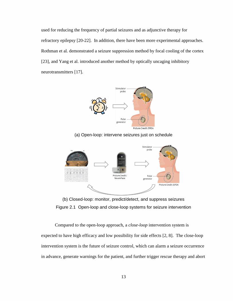
used for reducing the frequency of partial seizures and as adjunctive therapy for

refractory epilepsy [20-22]. In addition, there have been more experimental approaches.

Rothman et al. demonstrated a seizure suppression method by focal cooling of the cortex

[23], and Yang et al. introduced another method by optically uncaging inhibitory

neurotransmitters [17].

(a) Open-loop: intervene seizures just on schedule

(b) Closed-loop: monitor, predict/detect, and suppress seizures

Figure 2.1 Open-loop and close-loop systems for seizure intervention

Compared to the open-loop approach, a close-loop intervention system is

expected to have high efficacy and low possibility for side effects [2, 8]. The close-loop

intervention system is the future of seizure control, which can alarm a seizure occurrence

in advance, generate warnings for the patient, and further trigger rescue therapy and abort

14

the development of the seizure, such as by injecting fast-acting medication or turning on

a neuro-stimulator [1, 2, 8] (See Figure 2.1). When compared to open-loop systems that

work on schedule no matter when seizures occur or how frequently they strike, close-loop

systems may be superior in term of efficacy and safety, because they can help the rescue

therapy turn on effectively at certain necessary times and thus work with reduced amount

of medication [2]. It is noted that, however, it has not been clearly proven whether the

close-loop system indeed outperforms the open-loop system [1].

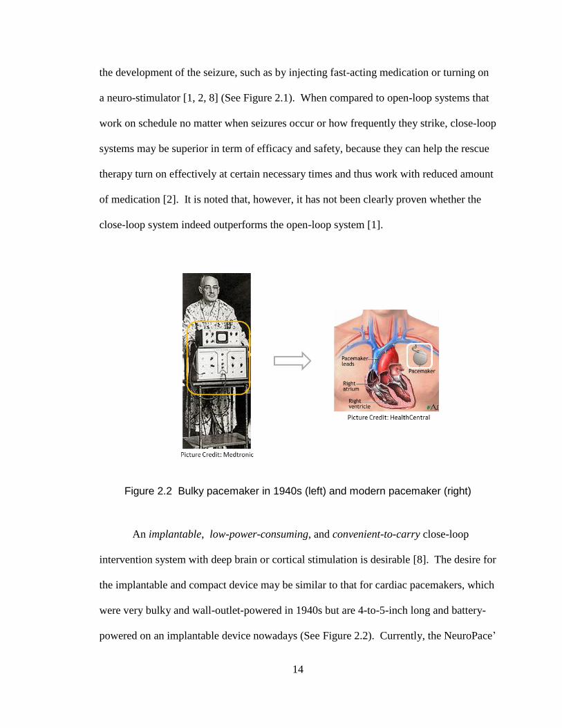
Figure 2.2 Bulky pacemaker in 1940s (left) and modern pacemaker (right)

An implantable, low-power-consuming, and convenient-to-carry close-loop

intervention system with deep brain or cortical stimulation is desirable [8]. The desire for

the implantable and compact device may be similar to that for cardiac pacemakers, which

were very bulky and wall-outlet-powered in 1940s but are 4-to-5-inch long and battery-

powered on an implantable device nowadays (See Figure 2.2). Currently, the NeuroPace’

15

RNS System [24], which is designed to detect a seizure and trigger electrical stimulation

runs on battery and is the one that is the closest to such a desirable close-loop system.

However, up to now, no seizure prediction algorithms have demonstrated enough

performance to be applied for the close-loop seizure intervention system [1].

When it comes to seizure prediction, certain signals have been observed that may

indicate a seizure approaching. Approximately 40% of temporal lobe epileptics have

some form of aura, a sensory perception that may indicate that a seizure is looming [25].

It has been claimed that some dogs have inborn ability to alert and/or respond to seizures

of the epileptics whom they serve for [26-29]. It is noted that the dogs’ ability is still

controversial. Epileptologists have observed a decrease in electroencephalogram (EEG)

prior to the onset of a seizure and have named the phenomenon the preictal quiescence or

the electrodecremental period [30]. There has been other technical evidence for the

possibility of seizure prediction, such as with Single-Photon Emission Computed

Tomography (SPECT) imaging [31] and with Electrocardiogram (ECG) [32-34].

However, the most popular technique for seizure prediction has been with EEG [1, 2] and

it will be explained in the following sub-chapter.

Prior Work in Seizure Prediction with EEG 2. 2

In short, to date, despite numerous claims that some approaches have significant

predictive power for seizures, seizure prediction is considered still illusive, like a “long

and winding road.” [1, 2]. Many of the prior researches on seizure prediction with EEG

16

were thoroughly reviewed by Mormann et al. [1]. Below is a summary of the prior

studies for seizure prediction with EEG.

Early Attempts with Linear Measures 2. 2. 1

Research on seeking seizure precursors started with surface EEG using linear measures in

the 1970s [35]. In the 1970s and 1980s, most researchers analyzed the precursors using

linear measures, such as spectral analysis and autoregressive modeling [36, 37]. Also,

characteristic changes in patterns of preictal spikes were attempted to be extracted [38],

but it turned out that they were not predictive on more extended databases, showing no

significant difference from interictal spikes [39].

Promising Nonlinear Analysis 2. 2. 2

After the advent of the chaos theory and development of novel nonlinear measures for

analyzing complex phenomena in the 1980s, nonlinear approaches for seizure prediction

research came into vogue. The nonlinear methods are expected to characterize a complex

dynamic system better than linear ones, especially where its outputs are hard to be

analyzed proportionally to its inputs, such as the weather. One of the most popularly

used nonlinear features in the 1990s was the largest Lyapunov exponent [40, 41]. Other

nonlinear measures that were promising in those times are as follows: correlation integral

[42], correlation density [43], correlation dimension [44], cross-correlation integral [45],

similarity index [46], and short-term maximum Lyapunov exponent [47]. It is noted that

those studies were considered incomplete in the sense that they focused on preictal

recordings and did not include an evaluation in interictal recordings.

17

Skepticism on Nonlinear Measures 2. 2. 3

After the approaches with nonlinear measures optimistically brought some partial success

in seizure prediction in the 1990s, however, the results from the nonlinear analysis were

questioned and challenged in the early 2000s. For example, correlation dimension and

integral were not able to reproduce their optimistic results in long recordings [48, 49].

Also, the robustness of the similarity index was challenged by later studies [50], and the

inability of Lyapunov exponents to predict seizures was demonstrated [51, 52].

Furthermore, many studies that have directly compared linear to nonlinear methods have

demonstrated that nonlinear analyses may not produce superior sensitivity and specificity

to the linear ones [11, 53, 54].

Main Barriers to Progress in Seizure Prediction Research 2. 2. 4

Despite a number of claims that an algorithm has significant predictive power over a long

window prior to a seizure, none has succeeded in a device with high sensitivity and

specificity. There are several putative reasons for this. The first is large variations in

EEG patterns between patients. This may be the main reason many false positives occur

when one generic algorithm was applied to patients [1, 55] Thus, seizure detectors or

predictors are better to be optimized for each patient [9, 10, 56]. Patient-specific

algorithms for seizure prediction are supposed to be the most beneficial for patients

suffering from recurrent seizures whose types and originations and EEG patterns are

similar. Second, most of the previous studies have focused on single features. While no

single linear or nonlinear feature has been found yet [1, 8], it may be possible that the

combination of the potential features or their essential subset would provide good

18

predictive power. Each of the measures presumably identifies some features of the

preictal EEG that distinguishes it from interictal one, and integrating them would lead to

high sensitivity and specificity. The last putative reason is methodological issues on

training and testing: in-sample optimization and out-of-sample testing [1]. In many of

prior studies, a training set and a test set were not perfectly separated, but the training set

is also included in testing. This may lead to an algorithm that is over-fitted, performing

very well with its database in that the result may be inflated so that the result may not

reflect that under the real situation. Thus, out-of-sample testing is necessary to prevent

the over-fitted results that may be too optimistic only in their own database.

Recent Research Trend in Seizure Prediction and 2. 3

Detection with EEG

Machine Learning Approaches 2. 3. 1

To date, many parts of the mechanism of how the brain works and how seizures develop

still remain unknown. One way to analyze unknown systems is by using machine

learning. Machine learning, which is a branch of artificial intelligence, is a computer-

based statistical discipline for the design and development of algorithms that allow

computers to learn a statistical model based on empirical data. Machine learning is

useful, specifically when given vast datasets it is difficult to know their pattern or to

generate descriptive or predictive models based on the datasets. It has been very widely

applied to many areas these days, spanning information technology, finance, and

marketing.

19

Recently, researchers in the society for seizure detection and prediction also

started using machine learning for their analysis. Gardner et al. used a one-class novelty

detection approach [57]. Also, Shoeb et al. have proposed SVM-based binary

classification approaches [56, 58]. Furthermore, Nandan et al. have compared the

performances resulting from use of different machine learning methods [59]. Chisci et al.

have combined machine-learning-based classification methods and statistical approaches

for postprocessing, such as using the Kalman filter [5, 60].

Machine learning has the following advantages for seizure detection and

prediction analysis. First, it can generate a descriptive or predictive statistical model,

even if a system’s operation is not clearly recognizable, like an unknown and having-

hidden-patterns “X” box. This is the significant advantage for seizure detection and

prediction analysis, considering that the seizure evolution mechanism is not clearly

understood yet. Second, machine learning approaches can generate patient-specific

models that can better fit to each patient’s EEG patterns than generic ones, since EEG

patterns significantly differ across subjects. Optimized by machine learning with each

patient’s recordings, seizure detectors and predictors may perform better for the patient

with higher sensitivity and specificity. Those machine-learning-based patient-specific

algorithms are expected to be the most beneficial for patients who suffer from recurrent

seizures with similar seizure types, originations, and EEG patterns. Lastly, machine

learning methods are inherently multivariate approaches. They establish a mapping

between inputs and outputs, no matter what dimensions the input samples have [14, 61].

For seizure prediction, no single measure that can perfectly indicate predictive power for

seizures has been found [1, 2]; however, each single measure may potentially identify

20

some preictal states [11]. Higher sensitivity and specificity may be achievable by

combining certain number of potential measures and machine learning approaches.

Commercial Efforts 2. 3. 2

Devices relevant to seizure detection and prediction applications have been under

development and presented by several companies. NeuroPace

(http://www.neuropace.com/) has developed the RNS that is designed for medically

refractory partial epilepsy and consists of neurostimulators as well as depth leads and

cortical strip leads (See Figure 2.3 (a)). Cyberonics’ (http://www.cyberonics.com/en/)

Vagus Nerve Stimulation Therapy has been approved for use in refractory epilepsy by the

U.S. Food and Drug Administration (See Figure 2.3 (b)). NeuroVista

(http://www.neurovista.com/) is making an implantable seizure advisory system as well

as an Epilepsy Management System. Medtronic (http://www.medtronic.com/) has

performed research on seizure detection [56] and implantable brain-disease-relevant

neuroprosthesis [62]. As listed above, there is growing industry interest for implantable

seizure detectors and predictor with low power consumption.

(a) NeuroPace’ RNS

(b) Cyberonics’ VNS Therapy

Figure 2.3 Commercial products for anti-seizure systems

21

Technical Backgrounds 2. 4

Moving Window Analysis 2. 4. 1

Moving window analysis is a temporal analysis method where certain linear or nonlinear

characterizing measures are calculated and extracted from a window of signals, such as

ECG or EEG, in a pre-defined length, and they subsequently continue from each of the

following windows. The pre-defined length typically ranges between 10 and 40 seconds

[1] and the overlap may exist between the neighbors of windows.

Figure 2.4 Moving window analysis with half-overlapped windows

Support Vector Machine Classification 2. 4. 2

The SVM is a maximum-margin statistical learning procedure where the descriptive or

predictive model is to be written on a subset of the training instances [63] (See Equation

2.1 and Figure 2.5). The goal of SVM-classification is to establish a mapping ,

using labeled training data ( ), i=1,2,…, p, where the input set and its

corresponding output is either of { }; and to classify the test set , j=1,2,…, q

where and may have the similar probability distribution as the training set. In

Figure 2.5 and Equation 2.1, is the hyperplane for classification, where

is the normal vector to the hyperplane and

‖ ‖ is the offset of the hyperplane from the

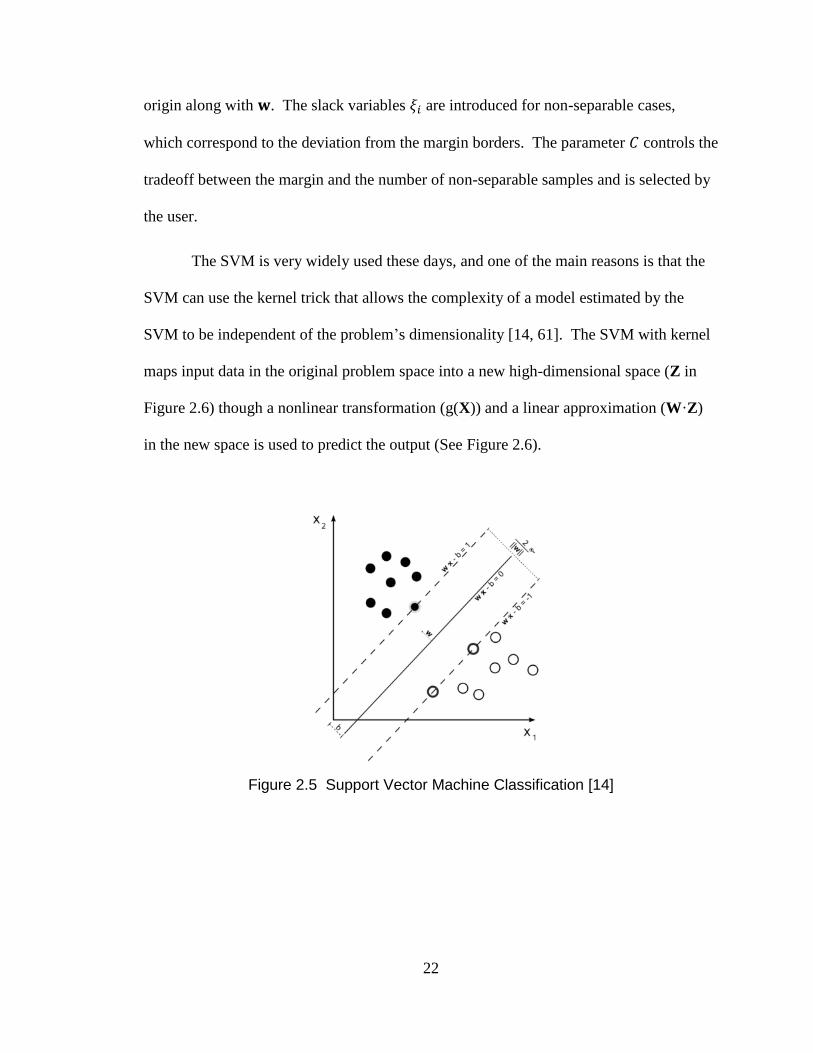
22

origin along with . The slack variables are introduced for non-separable cases,

which correspond to the deviation from the margin borders. The parameter controls the

tradeoff between the margin and the number of non-separable samples and is selected by

the user.

The SVM is very widely used these days, and one of the main reasons is that the

SVM can use the kernel trick that allows the complexity of a model estimated by the

SVM to be independent of the problem’s dimensionality [14, 61]. The SVM with kernel

maps input data in the original problem space into a new high-dimensional space (Z in

Figure 2.6) though a nonlinear transformation (g(X)) and a linear approximation (W·Z)

in the new space is used to predict the output (See Figure 2.6).

Figure 2.5 Support Vector Machine Classification [14]

23

‖ ‖ ∑

subject to the constraints: [( ) ]

Equation 2.1 Standard quadratic optimization problem of SVMs with soft margin

Figure 2.6 SVM’s mapping of inputs onto a high-dimensional space and linear

approximation for output prediction [14]

Figure 2.7 4-fold cross-validation

24

Cross-Validation 2. 4. 3

One desires that the statistics from a predictive model on a certain limited dataset

represents the actual statistics in practice. One of the simplest statistical methods to test

validity of a model is by cross-validation. Cross-validation is a statistical technique for

generating the generalized statistics from an analysis on limited data by resampling,

where the analysis is tested on independent datasets but evaluated across the entire

datasets [14, 64]. Practically, k-fold cross-validation is widely used (See Figure 2.7). In

k-fold cross-validation, first, the whole dataset is divided into k disjoint subsets of

approximately equal size. While a single subset is retained for evaluating a model,

mostly a predictive model, the model is estimated based on the remaining subsets as

training data. This process is repeated k times and then the k results from the folds are

generalized into a single estimation, such as by averaging. One extreme case of k-fold

cross-validation is leave-one-out where k equals the number of instances N: only one

sample is left out for evaluation and the other (N-1) samples are used in training and then

this is repeated N times.

Kalman Filter 2. 4. 4

Kalman-filtering is a statistical method that produces estimates that tend to be close to the

true values of measurements [65]. It uses measurements that have been measured over

time and may contain noise and measurement inaccuracies and produces values that have

a tendency to be close to the true values of the measurements. The Kalman filter has

been widely used in a variety of applications, such as autonomous navigation [66].

25

Throughout the dissertation, the two-stage discrete-time Kalman filter has been

used:

( )

( )

where is a noisy estimate of a state in a certain time window k; the true state of ;

the variance of noise that is uncorrelated in time and Gaussian-distributed with zero-

mean; and the change rate of . The original output may not undergo as rapid and

abrupt changes so that the change rate (time-derivative) of tends to be stable with

smooth transitions.

We can estimate and as follows:

Therefore, having a state vector [ ] , we establish a state-space model as

follows:

[

]

[ ]

where ( ) is the variability in the brain’s state (the process noise) and

( ) is the noise in our measurement of the state (the observation noise). These

26

two noise terms are assumed to be uncorrelated, and the covariance matrices Q and R in

the process noise and the observation noise, respectively, are assumed as follows:

[

]

It is noted that in the above state-space model the state transition model matrix T and the

observation model matrix O as follows:

[

]

[ ]

We put as the covariance of the estimation error. Then, and

denote the

covariance of the estimation error of before and after the measurement is taken into

account, respectively. Starting with an identical matrix I, covariance matrices and

, the Kalman filter gain K, and the estimates and , are updated as follows (refer

to Equations 5.11 to 5.16 in [65]:

(

)

( )

( )

27

Sensitivity, Specificity, False Positive Rate per Hour, and 2. 4. 5

False Positive Percentage

Sensitivity and specificity are widely used statistical measures in binary classification

tests. In binary classification problems, there are four possible cases, as shown in Table

2.1. For an actual positive sample, if it is predicted as positive correctly, the sample is a

true positive; if predicted as negative incorrectly, that is a false negative. For an actual

negative sample, if it is predicted as negative correctly, the sample is a true negative; if

predicted as positive incorrectly, that is a false positive. Sensitivity is a measure that

demonstrates the proportion of actual positive instances that are correctly classified as

such, and specificity is another measure that shows the proportion of actual negative

instances that are correctly classified as such. In other words,

and

, where TP, FN, FP, and TN represent the number of samples of true

positives, false negatives, false positives, and true negatives, respectively.

In the dissertation, sensitivity and false positive rate per hour and false positive

percentage in interictal recordings are used for classification performance evaluation, as

suggested by Mormann et al.[1]. As seizure prediction is seen as a binary classification

problem in the dissertation, TP is the number of preictal events predicted correctly; FN

that of failure of preictal alarms in actual preictal times; and FP that of falsely generated

preictal alarms in actual interictal times. Then, sensitivity (

) represents the

proportion of the preictal events in a patient that are classified correctly as such by the

proposed approach. The false alarm rate per hour and the false positive percentage in

28

interictal recordings demonstrate how many false alarms are expected by the proposed

algorithm.

Table 2.1 Confusion matrix

Actual Class

Predicted Class

Positive Negative

Positive True Positive (TP) False Negative

(FN)

Negative False Positive (FP) True Negative (TN)

Fβ-measure 2. 4. 6

While sensitivity, false positive rate per hour, and false positive percentage may

unambiguously quantify prediction algorithms’ performance, one may necessarily

demand a single measure to quantify how successfully the algorithms run. Furthermore,

in seizure prediction work, missing predictive alarms for actual seizure occurrence (false

negatives) is much more critical than generating false alarms (false positives), and

classifying ordinary states correctly (true negatives) is a minor issue. To this end, we

have proposed Fβ-measure as the single evaluation measure for seizure prediction:

( )

( ) , where TP, FN, and FP are the number of instances of true

positives, false negatives, and false positives, respectively.

Fβ-measure, also called as Fβ-score, is the harmonic mean of precision (

)

and recall (

) with more emphasis on precision: ( )

( ) .

29

It is a widely used measure, especially in the area of information retrieval in web queries

[67] and machine learning. It is noted that true negatives (TNs) are not taken into

account in the Fβ-measure.

Using the Fβ-measure for a single evaluation metric for prediction algorithms, we

have selected . By using the F2-measure, it is expected for FNs to be treated four

times more critically than FPs while TPs maintain their significance and TNs are ignored.

p-value 2. 4. 7

Sensitivity, false positive rate, false positive percentage in interictal recordings are

recommended to objectively demonstrate results from a seizure prediction algorithm [68].

However, using only those numbers, one cannot strictly determine if the algorithm’s

results are attributed to chance. Thus, to quantifiably demonstrate that statistics from an

algorithm are far from randomly generated ones, p-value is used in the dissertation. The

p-value is the probability of obtaining a test statistic as extreme or more extreme than the

one that is actually observed, assuming that the null hypothesis is true [64].

We have estimated the one-sided p-values that demonstrate how superior the

sensitivity of our algorithm is to chance [69]:

∑ ( )

( )

, for

where a proposed predictor correctly identifies of preictal events and is the

sensitivity of the corresponding chance predictor. It is noted that there are many

approaches to estimate the p-value for seizure prediction [69-71].

30

Receiver Operating Characteristic Analysis 2. 4. 8

Receiver operating characteristic (ROC) analysis is a simple but powerful visual

statistical method that uses a plot of true positive rate (

) as a function of

false positive rate (

) [72, 73]. It plots a curve, called as ROC curve, as a

discrimination threshold varies (See Figure 2.8). It has been widely used in binary

classification problems, especially in medical decision making [73].

In binary classification problems, the ROC analysis provides a simple way to

visualize a classifier’s performance and furthermore to quantify the performance. To

quantify classifiers’ performance as a single number in the ROC analysis, the area under

the curve (AUC) is used in general. The AUC integrates the area under the ROC curve

(See Figure 2.8). The perfect classifier produces an AUC of 1, because it results in a

TPR of 1 and FPR of 0. The poorest classifier produces an AUC of 0.5: the worst

classifier produces a diagonal ROC curve, where true and false decisions are equally

made, such as in tossing a fair coin. It is noted that better classifiers have their curve

approach closer to the upper-left corner in ROC analysis.

In short, graphically with the curve and numerically with the AUC, the ROC

analysis is an effective statistical tool to analyze provides a method to choose an optimal

classification model.

31

Figure 2.8 ROC curve and area under the curve

32

Chapter 3

Seizure Prediction with Spectral Power of

iEEG Using SVMs

Introduction 3. 1

There has been recently great progress in seizure suppression methods: for example, the

deep brain stimulation therapy in an open-loop approach has demonstrated its capability

of intervening seizures in clinical trials [7]. The efficacy of the open-loop method can be

improved by a closed-loop therapy, where a seizure prediction device monitors and

triggers the seizure abatement. However, no seizure prediction algorithm has been

developed yet that can demonstrate high and reproducible sensitivity and specificity

enough for clinical trials [1].

Seizure prediction using electroencephalogram (EEG) with high sensitivity and

specificity has been elusive, despite numerous claims that a proposed algorithm or

measure has provided significant predictive power. Especially, nonlinear features, which

33

are much more computationally intensive to be computed than linear features, have

turned out to be not significantly better than linear ones for seizure prediction and

furthermore not predictive at all when tested on long time series [48].

The problem about seizure prediction on EEG/iEEG is considered to be

complicated by a variety of EEG/iEEG patterns across patients and no single predictive

features have been discovered yet. Thus, we hypothesize that a patient-specific

classification method based on multiple features extracted from iEEG will achieve high

sensitivity and specificity. Our patient-specific approach to seizure prediction is based on

a machine learning algorithm, classifying binary classes of iEEG signals in preictal

(immediately prior to a seizure) and interictal (between seizures) periods (See Figure 3.1

and Figure 3.2). For prediction, we select linear multiple features rather than nonlinear

ones. It is because nonlinear features are too complex to be calculated in time and our

ultimate goal is to develop seizure prediction algorithms and architectures for an

implantable device. It is noted that the material in this chapter is based on our published

work [5, 9, 10].

34

Figure 3.1 Preictal, ictal, and interictal iEEG in Patient 17

Figure 3.2 Electrode positions for iEEG recordings in Patient 17 in the Freiburg

database [74]

35

Methods 3. 2

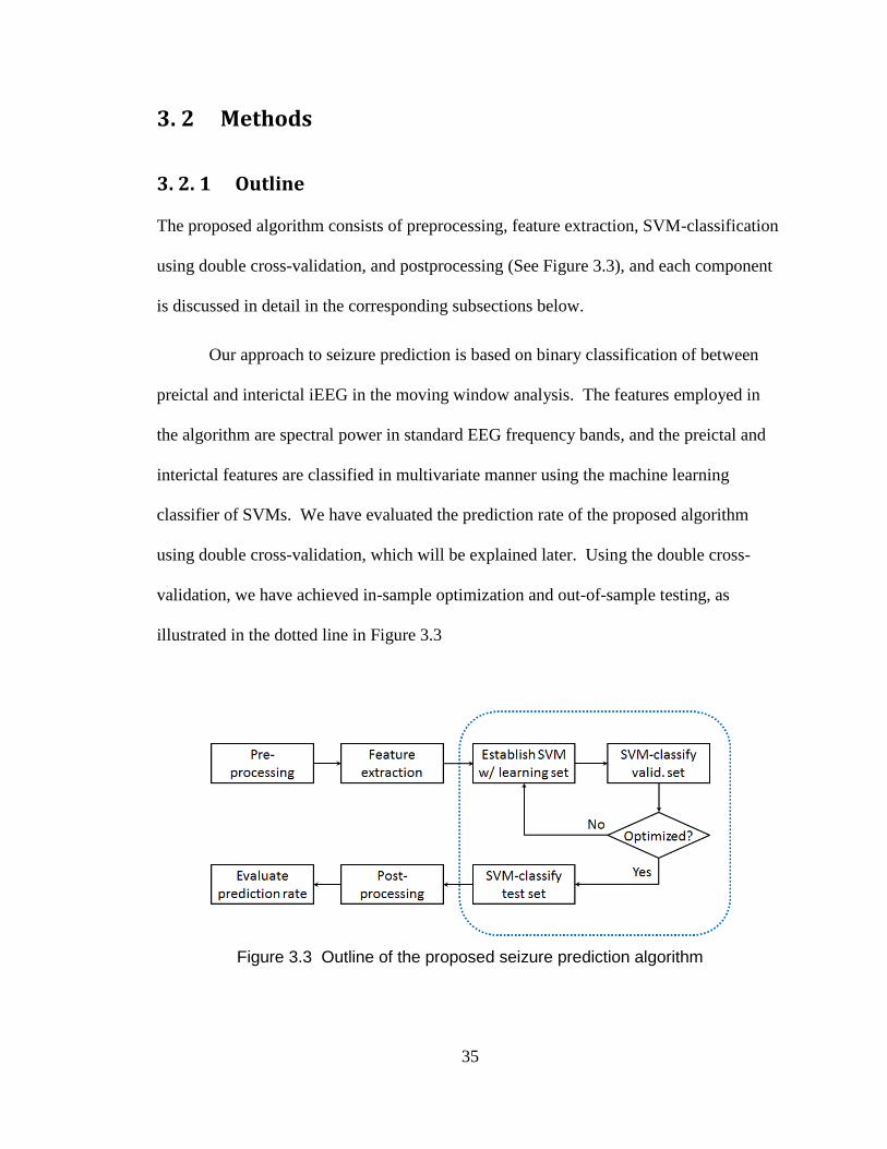
Outline 3. 2. 1

The proposed algorithm consists of preprocessing, feature extraction, SVM-classification

using double cross-validation, and postprocessing (See Figure 3.3), and each component

is discussed in detail in the corresponding subsections below.

Our approach to seizure prediction is based on binary classification of between

preictal and interictal iEEG in the moving window analysis. The features employed in

the algorithm are spectral power in standard EEG frequency bands, and the preictal and

interictal features are classified in multivariate manner using the machine learning

classifier of SVMs. We have evaluated the prediction rate of the proposed algorithm

using double cross-validation, which will be explained later. Using the double cross-

validation, we have achieved in-sample optimization and out-of-sample testing, as

illustrated in the dotted line in Figure 3.3

Figure 3.3 Outline of the proposed seizure prediction algorithm

36

Dataset Description 3. 2. 2

We have trained and tested our algorithm on the Freiburg EEG database

(https://epilepsy.uni-freiburg.de/freiburg-seizure-prediction-project/eeg-database), which

is open to any researcher by request. This database contains ECoG and iEEG recordings

from 21 patients who suffer from medically intractable focal epilepsy. We have chosen

18 out of the available datasets of 20 patients, which have three or more seizures.

The Freiburg database contains six ECoG/iEEG recordings from grid, strip or depth-

electrodes. The three electrodes were placed near the seizure focus (focal, illustrated in

solid red lines and numbered as 1 to 3 in Figure 3.1) and the other three were away from

the focus (extra-focal, illustrated in dotted blue lines and numbered as 4 to 6 in Figure

3.1). Seizure onset times were identified by certified epileptologists. The data were

collected at 256 Hz (Patient 12’s interictal at 512 Hz) sampling rate with 16 bit analog-to-

digital converters.

In our analysis, each 20-second-long window of iEEG recordings has been

categorized as ictal (containing a seizure), interictal (at least one hour preceding or

postceding a seizure), preictal (in 30 minutes preceding a seizure onset), or artifact. It is

noted that only preictal and interictal datasets are used for training SVMs.

Preprocessing: Removing Artifacts of iEEG Recordings 3. 2. 3

iEEG data are subject to artifacts, such as line noise, electrical noise, and movement

artifacts. Many of these artifacts may distort original iEEG and affect the further process

37

of training and testing. Thus, iEEG recordings with artifacts are removed from further

analysis. Artifacts in the Freiburg iEEG recordings were marked by epileptologists and

the information about the artifacts is provided along with the datasets. We have removed

windows that contain those artifacts in our analysis. The proportion of the removed

windows due to the artifacts to the overall recordings is negligible (approximately 10

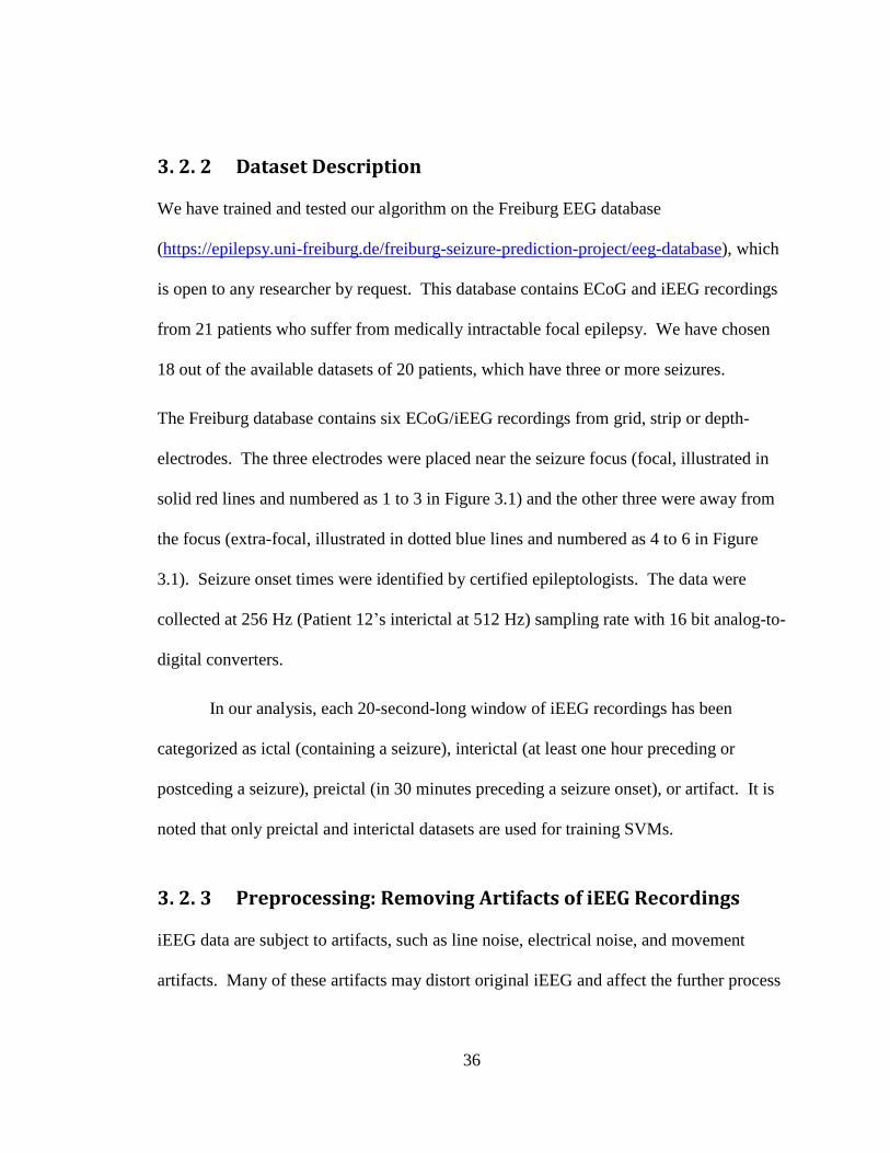
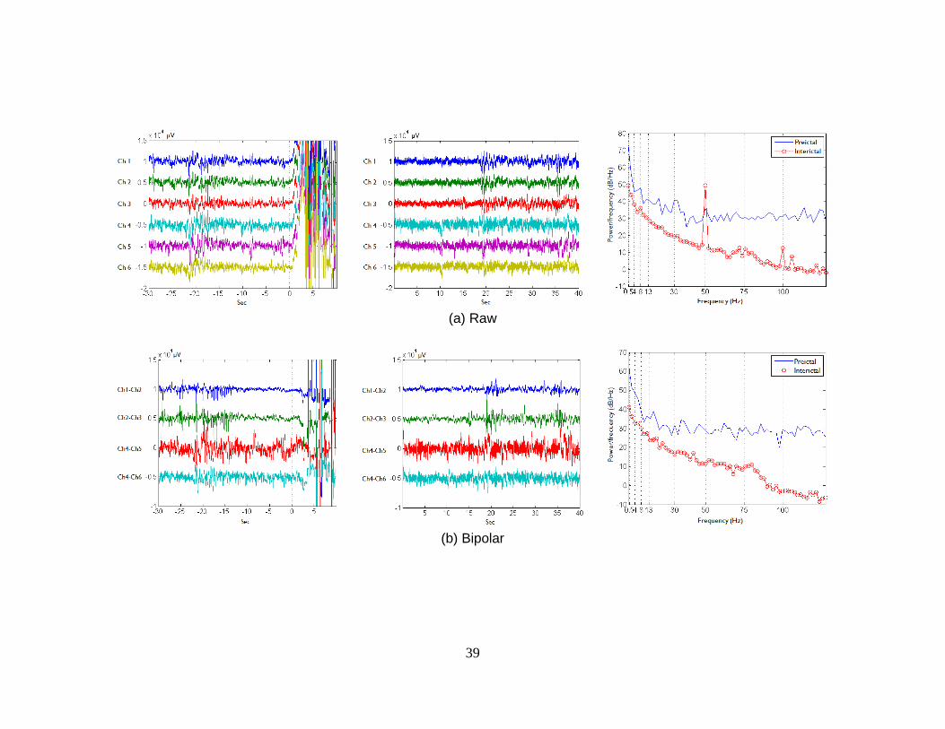
minutes in aggregate). Power line hums at 50Hz and 100Hz, which are illustrated in

Figure 3.4, have been removed by excluding spectral power in the bands of 47-53Hz and

97-103Hz when the features are extracted.

In addition, bipolar and/or time-differential methods have been used to remove or

reduce the effect of other types of artifacts in iEEG recordings (See Figure 3.4). The

bipolar (or space-differential) measurement provides common-mode rejection to reduce

line noise and movement artifacts that are common to all the electrodes. The bipolar

recording method is commonly used in the analysis of EEG and provides better spatial

resolution than that of ordinary reference recordings [75]. In our study, bipolar electrode

recordings are made preferentially between channels within focal or extra-focal and only

between the two groups if they are physical neighbors. This results in 4-6 bipolar

recordings for each patient: for example, in Patient 17’s recordings, where the electrode

positions were placed as shown in Figure 3.2, the bipolar iEEG recordings represent

differences in electrical potentials between Channels 1 and 2, 2 and 3, 4 and 5, and 4 and

6.

In general, raw iEEG demonstrates much more power in low frequency bands

than in high frequency bands, making it difficult to compare power across the bands. We

38

normalize the power in each band by measuring its contribution to the total power, and

the normalized power is dominated by small changes in power in low frequency bands.

Thus, the proportion of high frequency power in the total power is influenced by low

frequency power. The time-differential method (an approximate derivative in signals,

[ ] [ ] [ ]) provides a way to reduce that undesired effect, because the

time-differential preprocessing acts as a high-pass filter. Consequently, the time-

differential method makes power in the high frequency bands similar to that in low

frequency bands. It is noted that the time-differential processing is also known as the

Hjorth Mobility parameter [76].

Feature Extraction 3. 2. 4

We have calculated spectral power in 9 bands in a 20-second-long window of iEEG and

used it as a feature set in this study. We adopted the moving window analysis [1] with a

half overlap and it provides a prediction of a seizure every 10 seconds based on the

analysis of 5120 time points. Spectral bands are selected based on standard iEEG

frequency bands but the wide gamma band is split into four bands [9, 10]: delta (0.5-4Hz),

theta (4-8Hz), alpha (8-13Hz), beta (13-30Hz), four gamma bands (30-47Hz, 53-75Hz,

75-97Hz, and 103-128Hz, excluding power line hums), and their total (Refer to Figure

3.4). Power in each of the above bands is divided by the total power and the last feature

included is the total power [8].

39

(a) Raw

(b) Bipolar

40

(C) Time-differential

(d) Bipolar/Time-differential

Figure 3.4 Preictal iEEG (left column), interictal iEEG (middle), and their power spectral density (right) in the four different

preprocessing methods

41

iEEG data from each of the 6 electrodes are broken into 20-second windows that

half-overlap the previous one and 9 spectral features are extracted from each window.

Thus, a total of 54 features are extracted from every 10 seconds of raw or time-

differential iEEG recordings (27-48 features from bipolar or bipolar/time-differential).

Because we have four ways to preprocess iEEG, we will compare seizure prediction

based on each of the four preprocessing methods: raw, bipolar, time-differential, and

bipolar/time-differential.

SVM Classification Using Double Cross-Validation 3. 2. 5

Our classification task is to distinguish between two groups of iEEG spectral power

features in preictal and interictal. In our algorithm, the binary classification is performed

in two steps: SVM-classification with the 20-second window and postprocessing using

the Kalman filter (postprocessing will be explained in the next sub-section in detail).

The goal of SVM-classification is establishing and testing a mapping ( ) that is

from iEEG spectral features to either a preictal or interictal label. The mapping is

established using labeled training sets and tested to classify test sets that may have similar

probability distribution to the training sets.

Cost-sensitive SVMs (CSVMs) are used to handle the imbalance in number of

preictal and interictal samples (See Figure 3.5). Seizures are relatively rare: there is

approximately one preictal sample for every 10 interictal samples. Furthermore, we

consider it more significant to classify many preictal samples correctly than to have a few

false positives. CSVMs allow us to set misclassification costs of the preictal data higher

than that of interictal data.

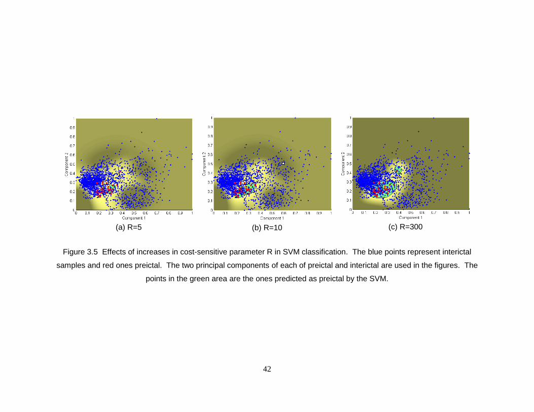
42

(a) R=5

(b) R=10

(c) R=300

Figure 3.5 Effects of increases in cost-sensitive parameter R in SVM classification. The blue points represent interictal

samples and red ones preictal. The two principal components of each of preictal and interictal are used in the figures. The

points in the green area are the ones predicted as preictal by the SVM.

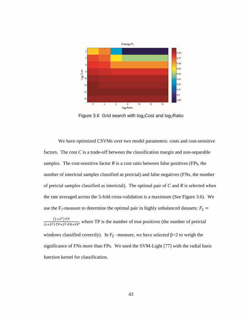
43

Figure 3.6 Grid search with log2Cost and log2Ratio

We have optimized CSVMs over two model parameters: costs and cost-sensitive

factors. The cost C is a trade-off between the classification margin and non-separable

samples. The cost-sensitive factor R is a cost ratio between false positives (FPs, the

number of interictal samples classified as preictal) and false negatives (FNs, the number

of preictal samples classified as interictal). The optimal pair of C and R is selected when

the rate averaged across the 5-fold cross-validation is a maximum (See Figure 3.6). We

use the F2-measure to determine the optimal pair in highly unbalanced datasets:

( )

( ) , where TP is the number of true positives (the number of preictal

windows classified correctly). In Fβ –measure, we have selected β=2 to weigh the

significance of FNs more than FPs. We used the SVM-Light [77] with the radial basis

function kernel for classification.

44

We desire that SVM-classification accuracy on the test data represents the actual

accuracy in practice. Many previous studies have trained and tested their prediction

models on the same datasets [1], resulting in overly optimistic prediction rates; their

models are not free from the over-fitting problem. Those prediction models, which may

be excessively fit to their datasets, may result in high sensitivity and specificity in their

data, but could not achieve those high rates in real conditions. To achieve an unbiased

prediction rate, we have used double cross-validation [13, 14] that ensures in-sample

optimization and out-of-sample testing.

The details of how we have performed double cross-validation are as follows. If a

patient has N seizures and I-hour-long interictal recordings, we separate the interictal

datasets into N blocks (folds), each of them approximately containing continuous (

)-

hour interictal recordings and pairing with each of 30-minute preictal datasets. It is noted

that interictal datasets are separated into different folds when they have a break in

recordings. We randomly choose one preictal and interictal fold and reserve it for testing

and use the other (N-1) folds for training: N-fold cross-validation. To establish an

optimal SVM classifier in training, we perform 5-fold cross-validation. We randomly

select 80% in the training set (the whole training set consists of (N-1) folds of preictal and

interictal) and establish a SVM model in the learning stage, and validate the model on the

remaining 20% of the training set to check if the model is well-fit (neither over-fit nor

under-fit). Once the SVM model is trained, the prediction rate is evaluated by testing the

model on the fold that was reserved for testing. This process is then repeated N times and

the average prediction rate is reported.

45

Postprocessing: Suppressing Isolated False Positives 3. 2. 6

Once a test set is SVM-classified, we have observed that FPs and FNs tend to be sporadic

and isolated in time as compared to TPs and TNs (true negatives, the number of interictal

windows classified correctly) [9, 10]. To eliminate these isolated FPs and FNs, we

postprocess the SVM-classification output using the two-stage discrete-time Kalman

filter (See Figure 3.7) [60, 65].

If the filtered output of the SVM though the Kalman filter is positive, only then do

we predict that a seizure will occur within the next 30 minutes. If no seizure occurs

within 30 minutes it is considered a false positive. We choose 30 minutes as our

prediction horizon, because we have defined preictal data as 30 minutes prior to a seizure

in training.

Additionally, we have tested a 4-of-7 analysis [9] and a 9-tap median filter for

postprocessing. The 4-of-7 analysis has been performed as follows. If there are 4 or

more positives out of 7 consecutive windows, then the prediction horizon following the

event is considered preictal; otherwise, it stays as interictal. The 9-tap median filter

produces the median value in 9 consecutive windows. If the median value is positive, the

prediction horizon is noted as preictal; otherwise, it is noted as interictal.

46

(a) testing in ictal recordings

(b) testing in interictal recordings

Figure 3.7 Examples of SVM classification and Kalman filter postprocessing in testing data (a) with ictal recordings and (b) with

interictal recordings

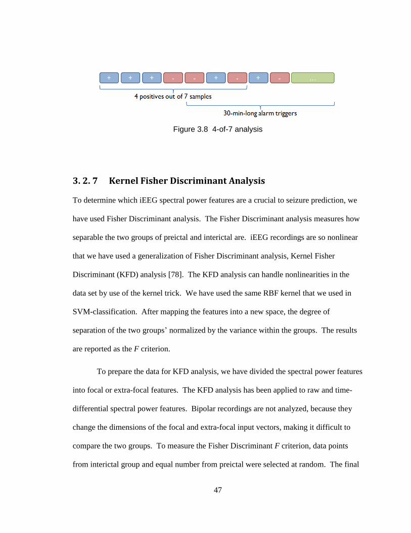
47

Figure 3.8 4-of-7 analysis

Kernel Fisher Discriminant Analysis 3. 2. 7

To determine which iEEG spectral power features are a crucial to seizure prediction, we

have used Fisher Discriminant analysis. The Fisher Discriminant analysis measures how

separable the two groups of preictal and interictal are. iEEG recordings are so nonlinear

that we have used a generalization of Fisher Discriminant analysis, Kernel Fisher

Discriminant (KFD) analysis [78]. The KFD analysis can handle nonlinearities in the

data set by use of the kernel trick. We have used the same RBF kernel that we used in

SVM-classification. After mapping the features into a new space, the degree of

separation of the two groups’ normalized by the variance within the groups. The results

are reported as the F criterion.

To prepare the data for KFD analysis, we have divided the spectral power features

into focal or extra-focal features. The KFD analysis has been applied to raw and time-

differential spectral power features. Bipolar recordings are not analyzed, because they

change the dimensions of the focal and extra-focal input vectors, making it difficult to

compare the two groups. To measure the Fisher Discriminant F criterion, data points

from interictal group and equal number from preictal were selected at random. The final

48

F criterion reported was averaged over many F’s calculated on different random

selections of preictal and interictal points. STPRtool (Statistical Pattern Recognition

Toolbox for Matlab, which is available at http://cmp.felk.cvut.cz/cmp/software/stprtool/)

has been used for our KFD analysis.

Results 3. 3

We have tested our patient-specific binary classification algorithm for seizure prediction

on iEEG recordings of 18 patients with 80 seizure events and 433.2 hours of interictal

recordings in the Freiburg EEG database. To evaluate the algorithm, we have measured

sensitivity, the false alarm rate per hour, and the percentage of interictal recordings

incorrectly classified as FPs.

Summary results for all the patients and all the four preprocessing methods are

shown in Table 3.1. Prediction using spectral power features calculated from raw iEEG

had total sensitivity of 93.8% (classifies 75 preictal events correctly out of 80) and 0.29

false positives per hour (125 false alarm events in 433.2 hours of interictal recordings),

resulting in a false prediction alarm for a total of 59.2 hours across all patients. Bipolar

preprocessing produced a higher sensitivity of 97.5% (78/80) and also an improvement

on the false positive rate of 0.27 per hour (118 false alarm events in 433.2 interictal

hours). Time-differential preprocessing led a significant improvement on the false

positive rate of 0.20 per hour (86 false alarm events in 433.2 hours), but did not improve

sensitivity (a sensitivity of 92.5%, 74/80). Prediction based on the combined two

preprocessing methods (bipolar/time-differential) demonstrated some improvement on

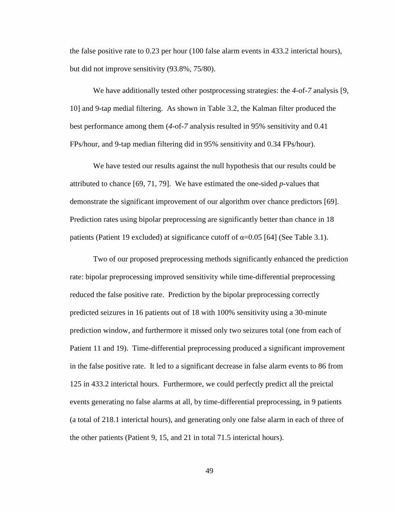
49

the false positive rate to 0.23 per hour (100 false alarm events in 433.2 interictal hours),

but did not improve sensitivity (93.8%, 75/80).

We have additionally tested other postprocessing strategies: the 4-of-7 analysis [9,

10] and 9-tap medial filtering. As shown in Table 3.2, the Kalman filter produced the

best performance among them (4-of-7 analysis resulted in 95% sensitivity and 0.41

FPs/hour, and 9-tap median filtering did in 95% sensitivity and 0.34 FPs/hour).

We have tested our results against the null hypothesis that our results could be

attributed to chance [69, 71, 79]. We have estimated the one-sided p-values that

demonstrate the significant improvement of our algorithm over chance predictors [69].

Prediction rates using bipolar preprocessing are significantly better than chance in 18

patients (Patient 19 excluded) at significance cutoff of α=0.05 [64] (See Table 3.1).

Two of our proposed preprocessing methods significantly enhanced the prediction

rate: bipolar preprocessing improved sensitivity while time-differential preprocessing

reduced the false positive rate. Prediction by the bipolar preprocessing correctly

predicted seizures in 16 patients out of 18 with 100% sensitivity using a 30-minute

prediction window, and furthermore it missed only two seizures total (one from each of

Patient 11 and 19). Time-differential preprocessing produced a significant improvement

in the false positive rate. It led to a significant decrease in false alarm events to 86 from

125 in 433.2 interictal hours. Furthermore, we could perfectly predict all the preictal

events generating no false alarms at all, by time-differential preprocessing, in 9 patients

(a total of 218.1 interictal hours), and generating only one false alarm in each of three of

the other patients (Patient 9, 15, and 21 in total 71.5 interictal hours).

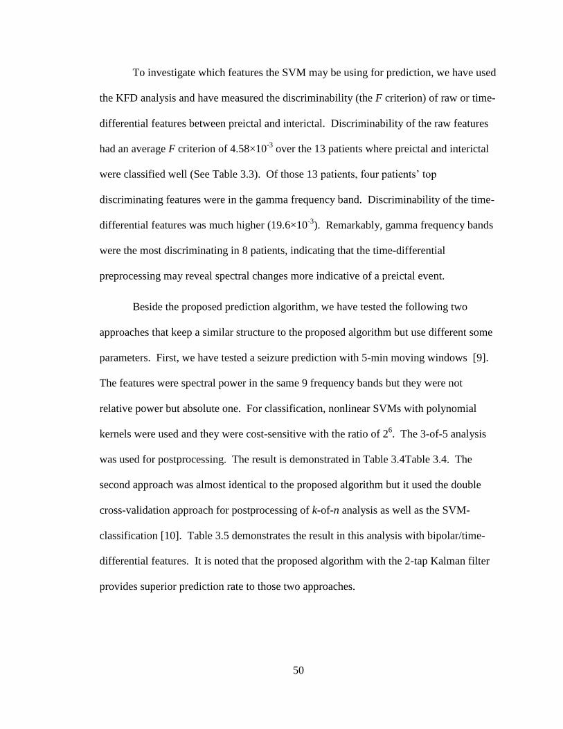
50

To investigate which features the SVM may be using for prediction, we have used

the KFD analysis and have measured the discriminability (the F criterion) of raw or time-

differential features between preictal and interictal. Discriminability of the raw features

had an average F criterion of 4.58×10-3

over the 13 patients where preictal and interictal

were classified well (See Table 3.3). Of those 13 patients, four patients’ top

discriminating features were in the gamma frequency band. Discriminability of the time-

differential features was much higher (19.6×10-3

). Remarkably, gamma frequency bands

were the most discriminating in 8 patients, indicating that the time-differential

preprocessing may reveal spectral changes more indicative of a preictal event.

Beside the proposed prediction algorithm, we have tested the following two

approaches that keep a similar structure to the proposed algorithm but use different some

parameters. First, we have tested a seizure prediction with 5-min moving windows [9].

The features were spectral power in the same 9 frequency bands but they were not

relative power but absolute one. For classification, nonlinear SVMs with polynomial

kernels were used and they were cost-sensitive with the ratio of 26. The 3-of-5 analysis

was used for postprocessing. The result is demonstrated in Table 3.4Table 3.4. The

second approach was almost identical to the proposed algorithm but it used the double

cross-validation approach for postprocessing of k-of-n analysis as well as the SVM-

classification [10]. Table 3.5 demonstrates the result in this analysis with bipolar/time-

differential features. It is noted that the proposed algorithm with the 2-tap Kalman filter

provides superior prediction rate to those two approaches.

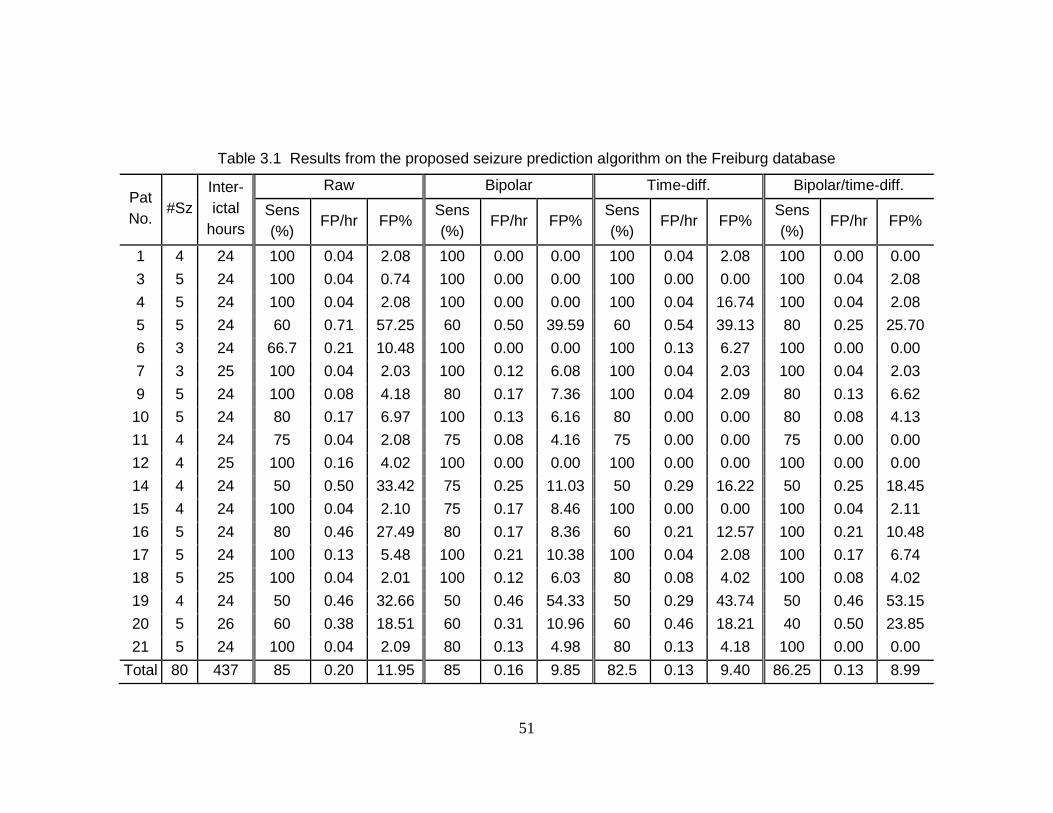
51

Table 3.1 Results from the proposed seizure prediction algorithm on the Freiburg database

Pat

No. #Sz

Inter-

ictal

hours

Raw Bipolar Time-diff. Bipolar/time-diff.

Sens

(%) FP/hr FP%

Sens

(%) FP/hr FP%

Sens

(%) FP/hr FP%

Sens

(%) FP/hr FP%

1 4 24 100 0.04 2.08 100 0.00 0.00 100 0.04 2.08 100 0.00 0.00

3 5 24 100 0.04 0.74 100 0.00 0.00 100 0.00 0.00 100 0.04 2.08

4 5 24 100 0.04 2.08 100 0.00 0.00 100 0.04 16.74 100 0.04 2.08

5 5 24 60 0.71 57.25 60 0.50 39.59 60 0.54 39.13 80 0.25 25.70

6 3 24 66.7 0.21 10.48 100 0.00 0.00 100 0.13 6.27 100 0.00 0.00

7 3 25 100 0.04 2.03 100 0.12 6.08 100 0.04 2.03 100 0.04 2.03

9 5 24 100 0.08 4.18 80 0.17 7.36 100 0.04 2.09 80 0.13 6.62

10 5 24 80 0.17 6.97 100 0.13 6.16 80 0.00 0.00 80 0.08 4.13

11 4 24 75 0.04 2.08 75 0.08 4.16 75 0.00 0.00 75 0.00 0.00

12 4 25 100 0.16 4.02 100 0.00 0.00 100 0.00 0.00 100 0.00 0.00

14 4 24 50 0.50 33.42 75 0.25 11.03 50 0.29 16.22 50 0.25 18.45

15 4 24 100 0.04 2.10 75 0.17 8.46 100 0.00 0.00 100 0.04 2.11

16 5 24 80 0.46 27.49 80 0.17 8.36 60 0.21 12.57 100 0.21 10.48

17 5 24 100 0.13 5.48 100 0.21 10.38 100 0.04 2.08 100 0.17 6.74

18 5 25 100 0.04 2.01 100 0.12 6.03 80 0.08 4.02 100 0.08 4.02

19 4 24 50 0.46 32.66 50 0.46 54.33 50 0.29 43.74 50 0.46 53.15

20 5 26 60 0.38 18.51 60 0.31 10.96 60 0.46 18.21 40 0.50 23.85

21 5 24 100 0.04 2.09 80 0.13 4.98 80 0.13 4.18 100 0.00 0.00

Total 80 437 85 0.20 11.95 85 0.16 9.85 82.5 0.13 9.40 86.25 0.13 8.99

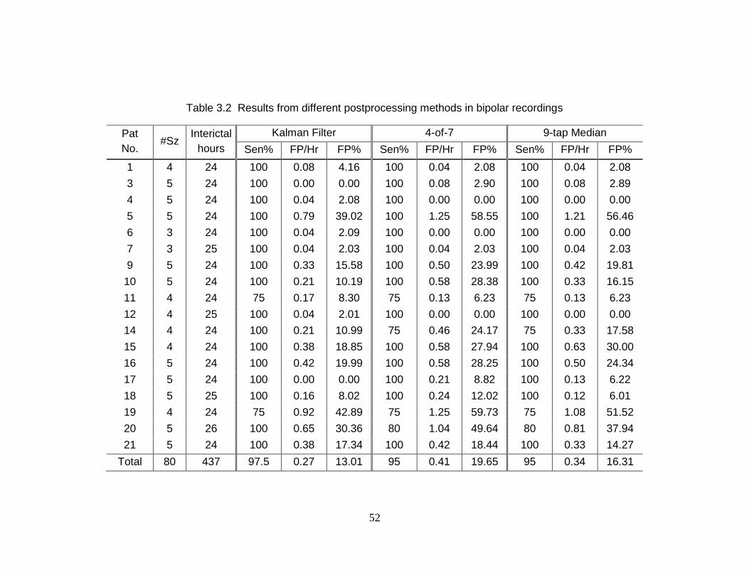
52

Table 3.2 Results from different postprocessing methods in bipolar recordings

Pat

No. #Sz

Interictal

hours

Kalman Filter 4-of-7 9-tap Median

Sen% FP/Hr FP% Sen% FP/Hr FP% Sen% FP/Hr FP%

1 4 24 100 0.08 4.16 100 0.04 2.08 100 0.04 2.08

3 5 24 100 0.00 0.00 100 0.08 2.90 100 0.08 2.89

4 5 24 100 0.04 2.08 100 0.00 0.00 100 0.00 0.00

5 5 24 100 0.79 39.02 100 1.25 58.55 100 1.21 56.46

6 3 24 100 0.04 2.09 100 0.00 0.00 100 0.00 0.00

7 3 25 100 0.04 2.03 100 0.04 2.03 100 0.04 2.03

9 5 24 100 0.33 15.58 100 0.50 23.99 100 0.42 19.81

10 5 24 100 0.21 10.19 100 0.58 28.38 100 0.33 16.15

11 4 24 75 0.17 8.30 75 0.13 6.23 75 0.13 6.23

12 4 25 100 0.04 2.01 100 0.00 0.00 100 0.00 0.00

14 4 24 100 0.21 10.99 75 0.46 24.17 75 0.33 17.58

15 4 24 100 0.38 18.85 100 0.58 27.94 100 0.63 30.00

16 5 24 100 0.42 19.99 100 0.58 28.25 100 0.50 24.34

17 5 24 100 0.00 0.00 100 0.21 8.82 100 0.13 6.22

18 5 25 100 0.16 8.02 100 0.24 12.02 100 0.12 6.01

19 4 24 75 0.92 42.89 75 1.25 59.73 75 1.08 51.52

20 5 26 100 0.65 30.36 80 1.04 49.64 80 0.81 37.94

21 5 24 100 0.38 17.34 100 0.42 18.44 100 0.33 14.27

Total 80 437 97.5 0.27 13.01 95 0.41 19.65 95 0.34 16.31

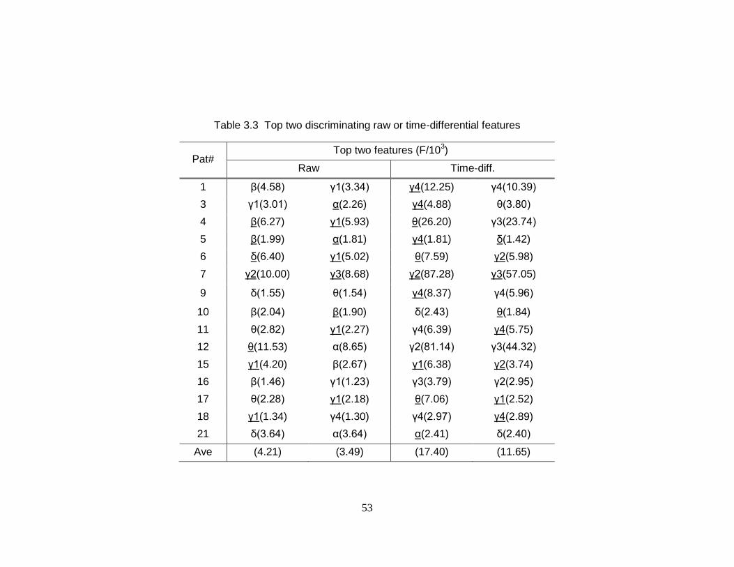
53

Table 3.3 Top two discriminating raw or time-differential features

Pat# Top two features (F/10

3)

Raw Time-diff.

1 β(4.58) γ1(3.34) γ4(12.25) γ4(10.39)

3 γ1(3.01) α(2.26) γ4(4.88) θ(3.80)

4 β(6.27) γ1(5.93) θ(26.20) γ3(23.74)

5 β(1.99) α(1.81) γ4(1.81) δ(1.42)

6 δ(6.40) γ1(5.02) θ(7.59) γ2(5.98)

7 γ2(10.00) γ3(8.68) γ2(87.28) γ3(57.05)

9 δ(1.55) θ(1.54) γ4(8.37) γ4(5.96)

10 β(2.04) β(1.90) δ(2.43) θ(1.84)

11 θ(2.82) γ1(2.27) γ4(6.39) γ4(5.75)

12 θ(11.53) α(8.65) γ2(81.14) γ3(44.32)

15 γ1(4.20) β(2.67) γ1(6.38) γ2(3.74)

16 β(1.46) γ1(1.23) γ3(3.79) γ2(2.95)

17 θ(2.28) γ1(2.18) θ(7.06) γ1(2.52)

18 γ1(1.34) γ4(1.30) γ4(2.97) γ4(2.89)

21 δ(3.64) α(3.64) α(2.41) δ(2.40)

Ave (4.21) (3.49) (17.40) (11.65)

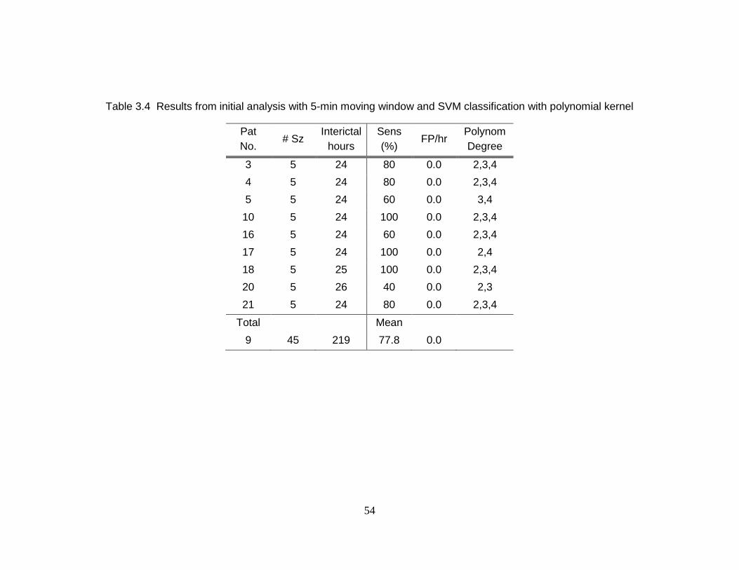
54

Table 3.4 Results from initial analysis with 5-min moving window and SVM classification with polynomial kernel

Pat

No. # Sz

Interictal

hours

Sens

(%) FP/hr

Polynom

Degree

3 5 24 80 0.0 2,3,4

4 5 24 80 0.0 2,3,4

5 5 24 60 0.0 3,4

10 5 24 100 0.0 2,3,4

16 5 24 60 0.0 2,3,4

17 5 24 100 0.0 2,4

18 5 25 100 0.0 2,3,4

20 5 26 40 0.0 2,3

21 5 24 80 0.0 2,3,4

Total

Mean

9 45 219 77.8 0.0

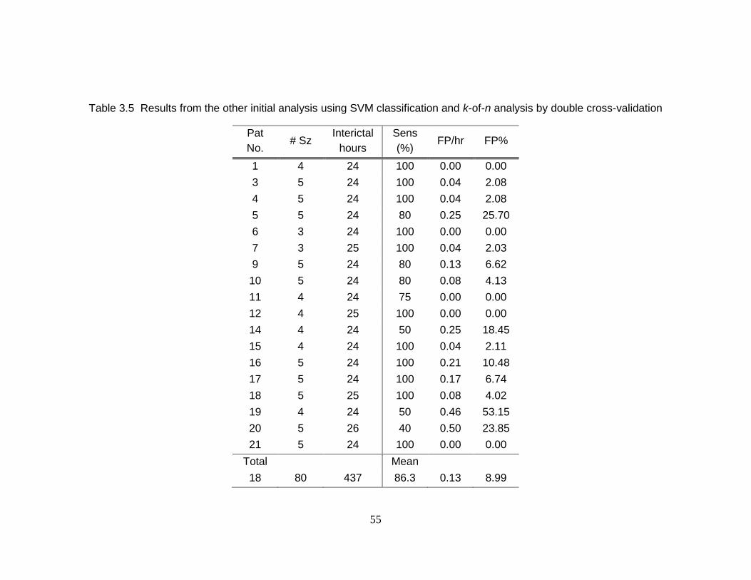
55

Table 3.5 Results from the other initial analysis using SVM classification and k-of-n analysis by double cross-validation

Pat

No. # Sz

Interictal

hours

Sens

(%) FP/hr FP%

1 4 24 100 0.00 0.00

3 5 24 100 0.04 2.08

4 5 24 100 0.04 2.08

5 5 24 80 0.25 25.70

6 3 24 100 0.00 0.00

7 3 25 100 0.04 2.03

9 5 24 80 0.13 6.62

10 5 24 80 0.08 4.13

11 4 24 75 0.00 0.00

12 4 25 100 0.00 0.00

14 4 24 50 0.25 18.45

15 4 24 100 0.04 2.11

16 5 24 100 0.21 10.48

17 5 24 100 0.17 6.74

18 5 25 100 0.08 4.02

19 4 24 50 0.46 53.15

20 5 26 40 0.50 23.85

21 5 24 100 0.00 0.00

Total

Mean

18 80 437 86.3 0.13 8.99

56

Discussions 3. 4

High sensitivity of 97.5% and the low false positive trigger rate of 0.27 per hour in

bipolar iEEG recordings in 18 patients demonstrate that seizures may be predicted using

the patient-specific approach of SVM-classification of spectral power features. We

expect this patient-specific methodology to be more successful for some patients than

others; patients who suffer from repeatable and stereotypical seizures are the easiest to

predict with this algorithm. By contrast, our machine learning approach may not succeed

in patients whose seizures evolve rapidly over time or in patients that express several

different types of seizures.

Our results may be compared directly to several other studies that have tested

prediction algorithms using the same Freiburg EEG database [1, 49, 80, 81]. We

demonstrate high sensitivity and specificity for this database yet reported. Furthermore,

we have used in-sample optimization and assessed the results with out-of-sample testing

(a test set is never involved in training) through the use of double cross-validation.

While some studies may present higher sensitivity and/or specificity than ours [1], their

algorithms were trained and tested on the exact same datasets; therefore, the results are

not directly comparable.

Another seizure prediction algorithm has been recently introduced using

autoregressive coefficients and SVM-classification and demonstrated a high prediction

rate [60]; our algorithm is the first to be tested using double-cross validation in that all the

datasets were resampled and tested and using the prediction horizon as defined by the

57

International Seizure Prediction Workshop (IWSP4, http://www.iwsp4.org/). The

standard of the IWSP4 for prediction horizon is that once a seizure prediction has been

issued it is required to be left on for the entire duration of the prediction horizon.

An important feature of our algorithm is that it analyzes linear features with a

nonlinear classifier. With respect to implementing it in an implantable device, the use of

linear features is attractive because they can be calculated rapidly and with low power

consumption when compared to nonlinear features. For classification, we used SVMs

with the nonlinear kernel that may require high power consumption, but the nonlinear

SVMs may be replaced by linear SVMs that consumes much less power [56] (See Figure

3.9). Seizure prediction using linear SVMs will be discussed in detail in the next chapter.

In this chapter, we trained and tested the algorithm after removal of artifacts.

Artifacts in iEEG may negatively affect our seizure prediction algorithm and may

decrease sensitivity and specificity in a real device. An additional but simple algorithm

may be necessary in practice to identify the artifacts such as out-of-measurement-range or

electrode disconnect in real-time.

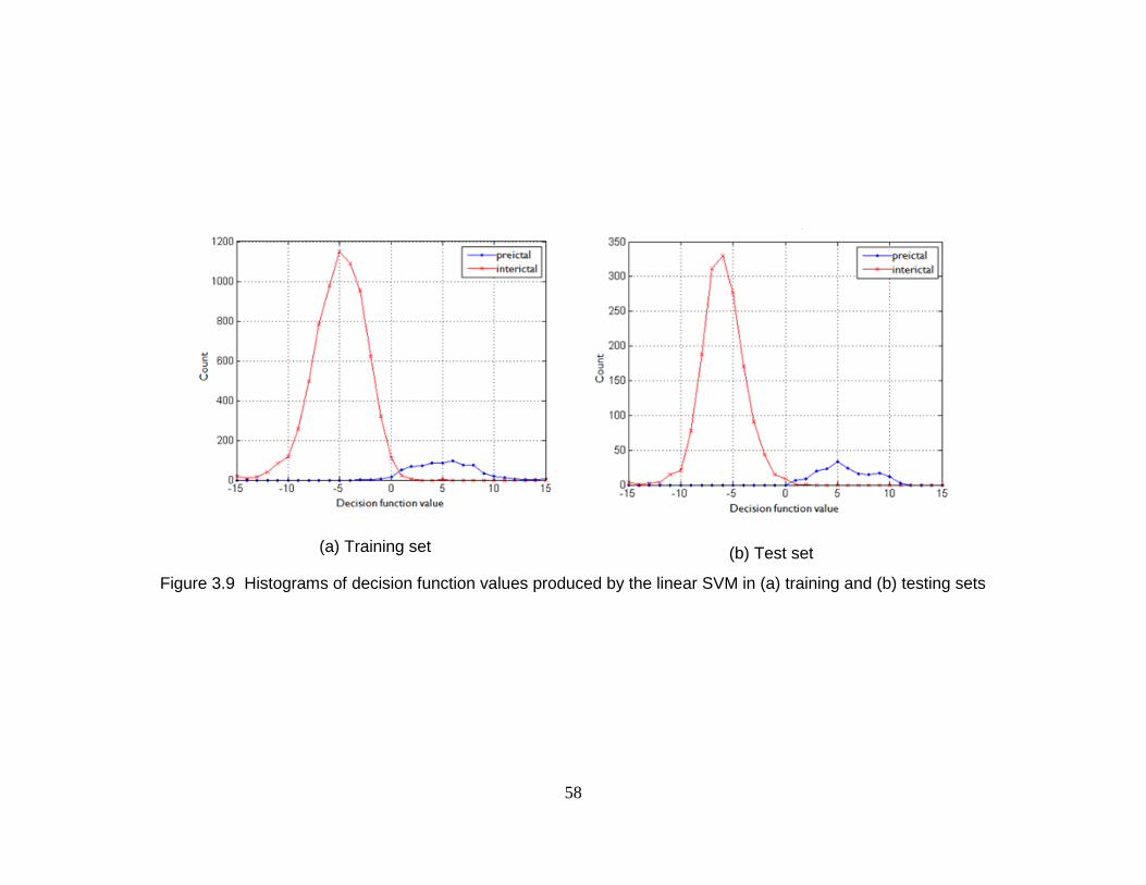
58

(a) Training set

(b) Test set

Figure 3.9 Histograms of decision function values produced by the linear SVM in (a) training and (b) testing sets

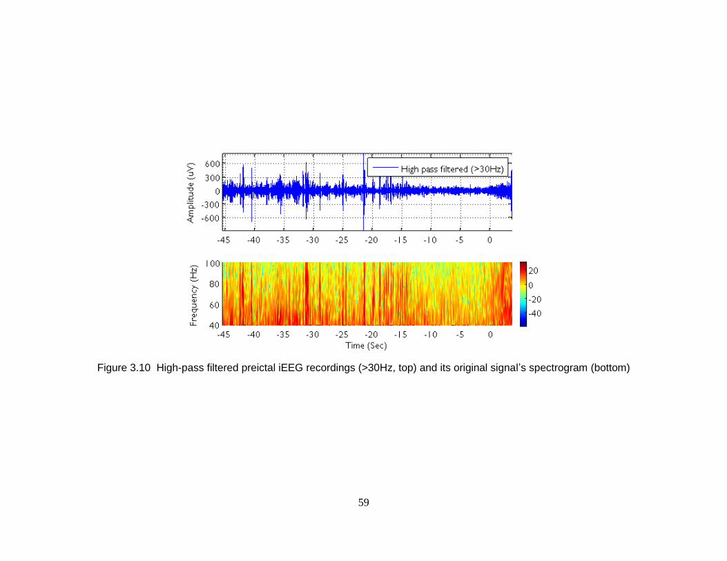
59

Figure 3.10 High-pass filtered preictal iEEG recordings (>30Hz, top) and its original signal’s spectrogram (bottom)

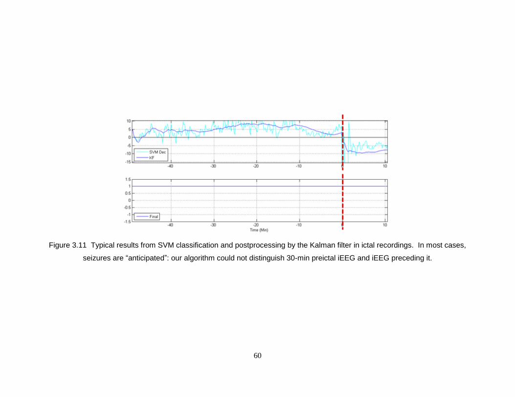
60

Figure 3.11 Typical results from SVM classification and postprocessing by the Kalman filter in ictal recordings. In most cases,

seizures are “anticipated”: our algorithm could not distinguish 30-min preictal iEEG and iEEG preceding it.

61

KFD analysis of the features suggests that the SVM may predict seizures by

detecting changes in gamma band power with respect to the total power. While it has

already been shown that power changes in gamma bands occur prior to a seizure and can

be used for prediction [11], our results demonstrate that using those power changes in a

multivariate approach may lead to much higher sensitivity and specificity. It is noted that

the increase in gamma band power may be due to spontaneous iEEG spike bursts

occurring more frequently rather than the emergence of intermittent rhythmic gamma

waveforms (See Figure 3.10). We expect that seizure prediction may improve if iEEG

sampling rates are increased to detect changes in even higher frequency ranges.

The use of bipolar and/or time-differential preprocessing increased sensitivity and

decreased false positive rates when compared to results from raw iEEG. Bipolar

preprocessing reduces noise through common mode rejection. Time-differential

preprocessing acts as a high filter and thus it flattens the spectrum reducing the

dominance of the low-frequency power on the total power. The use of both bipolar and

time-differential methods provided low false positive rate without decreasing sensitivity.

Seizure prediction may be further improved by optimal selection of preictal data

for training the SVM algorithm. In this chapter, we have operationally defined preictal as

any data that occurred 30 minutes prior to a seizure. Our algorithm successfully

distinguished iEEG in 30 minutes prior to the seizures from interictal recordings. This

indicates that a heightened seizure state could be detected, but it could not be determined

if that change of states occurs at a certain finite time prior to the seizures. When our

classifier was applied to the iEEG recordings that contain ones immediately preceding

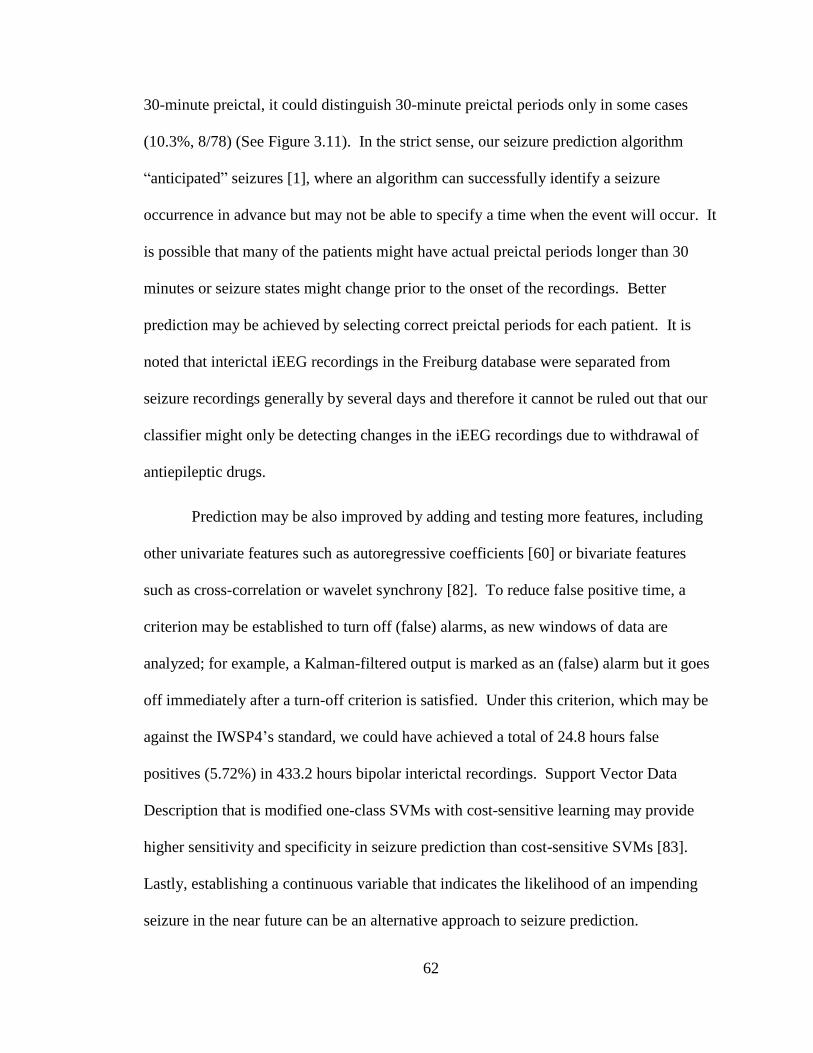
62

30-minute preictal, it could distinguish 30-minute preictal periods only in some cases

(10.3%, 8/78) (See Figure 3.11). In the strict sense, our seizure prediction algorithm

“anticipated” seizures [1], where an algorithm can successfully identify a seizure

occurrence in advance but may not be able to specify a time when the event will occur. It

is possible that many of the patients might have actual preictal periods longer than 30

minutes or seizure states might change prior to the onset of the recordings. Better

prediction may be achieved by selecting correct preictal periods for each patient. It is

noted that interictal iEEG recordings in the Freiburg database were separated from

seizure recordings generally by several days and therefore it cannot be ruled out that our

classifier might only be detecting changes in the iEEG recordings due to withdrawal of

antiepileptic drugs.

Prediction may be also improved by adding and testing more features, including

other univariate features such as autoregressive coefficients [60] or bivariate features

such as cross-correlation or wavelet synchrony [82]. To reduce false positive time, a

criterion may be established to turn off (false) alarms, as new windows of data are

analyzed; for example, a Kalman-filtered output is marked as an (false) alarm but it goes

off immediately after a turn-off criterion is satisfied. Under this criterion, which may be

against the IWSP4’s standard, we could have achieved a total of 24.8 hours false

positives (5.72%) in 433.2 hours bipolar interictal recordings. Support Vector Data

Description that is modified one-class SVMs with cost-sensitive learning may provide

higher sensitivity and specificity in seizure prediction than cost-sensitive SVMs [83].

Lastly, establishing a continuous variable that indicates the likelihood of an impending

seizure in the near future can be an alternative approach to seizure prediction.

63

Conclusion 3. 5

A patient-specific algorithm for seizure prediction is proposed that is based on the binary

classification of preictal and interictal, using multiple features of spectral power from

iEEG and SVM classification. The spectral power features are extracted from raw or

bipolar-and/or-time-differential iEEG in 20-sec long windows with half-overlap. SVMs

classify those features into either a preictal or an interictal class, and in order to collect

preictal samples more, cost-sensitive SVMs are used. To reduce the number of false

positives, the Kalman filter is applied for postprocessing. The proposed algorithm is

evaluated in 18 subjects’ recordings on the Freiburg EEG database. It achieves high

sensitivity of 97.5% with total 80 seizures, a low false alarm rate of 0.27 per hour, and

false prediction times of 13.0% over a total of 433.2 interictal hours by bipolar

preprocessing. By time-differential preprocessing, it produces high sensitivity of 92.5%,

a false positive rate of 0.20 per hour, and false prediction times of 9.5%. Those results

have been achieved in in-sample optimization and out-of-sample testing approach, using

the double cross-validation method. The high prediction rates demonstrate that seizure

can be predicted by the patient-specific approach using linear features of spectral power.

64

Chapter 4

Reduced-Complexity Seizure Prediction

with EEG

Introduction 4. 1

In the last chapter, we demonstrated that our seizure prediction algorithm that uses 27-54

spectral power features, nonlinear SVMs, and the Kalman filter can produce high

sensitivity and low false positive rate. For the seizure prediction algorithm, we selected

spectral power as a feature, because it is linear and therefore advantageous with respect to

implementing it in an implantable device.

However, when it comes to designing an actual implantable device, the algorithm

proposed in the last chapter may suffer from the three disadvantages of (1) the large

number of features (27-54), (2) nonlinear SVMs, and (3) the Kalman filter, due to their

high complexity and therefore high power consumption in the device. For example, it

65

was demonstrated in [56, 84] that a seizure alert algorithm on an FPGA device that

extracts four spectral power features and uses nonlinear SVM classification may not meet

the power consumption constraint for being implantable. In this sense, 27-54 features

may be too many and the complexity of both the nonlinear SVMs and the Kalman filter

may be too large for an implantable device. Therefore, in this chapter, we investigate a

small number of key features that can produce high sensitivity and low false positive rate.

Furthermore, we investigate how the nonlinear SVMs and the Kalman filters can be

replaced by linear SVMs and linear filters. Finally, a reduced complexity prediction

algorithm is proposed that extracts only 6-9 features and uses the linear SVM classifier

and a moving-average filter (See Figure 4.1).

Methods 4. 2

Overview 4. 2. 1

The main method used for identifying minimal set of key features is recursive feature

elimination using SVMs (RFE SVM) [85, 86]. RFE SVM is a feature subset selection

technique using backward feature elimination (See Figure 4.2) and demonstrates an

excellent advantage over the other feature selection techniques as follows. In the

selection process, RFE SVM uses interaction with the classifier of linear SVMs that are

to be used in the classification followed by the selection [86]. We have used two-step

RFE SVM analysis to investigate small numbers of key features: coarse grained search

by 9-feature elimination per iteration and then fine grained search by 3-feature

elimination per iteration.

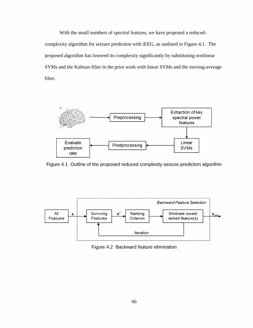
66

With the small numbers of spectral features, we have proposed a reduced-

complexity algorithm for seizure prediction with iEEG, as outlined in Figure 4.1. The

proposed algorithm has lowered its complexity significantly by substituting nonlinear

SVMs and the Kalman filter in the prior work with linear SVMs and the moving-average

filter.

Figure 4.1 Outline of the proposed reduced complexity seizure prediction algorithm

Figure 4.2 Backward feature elimination

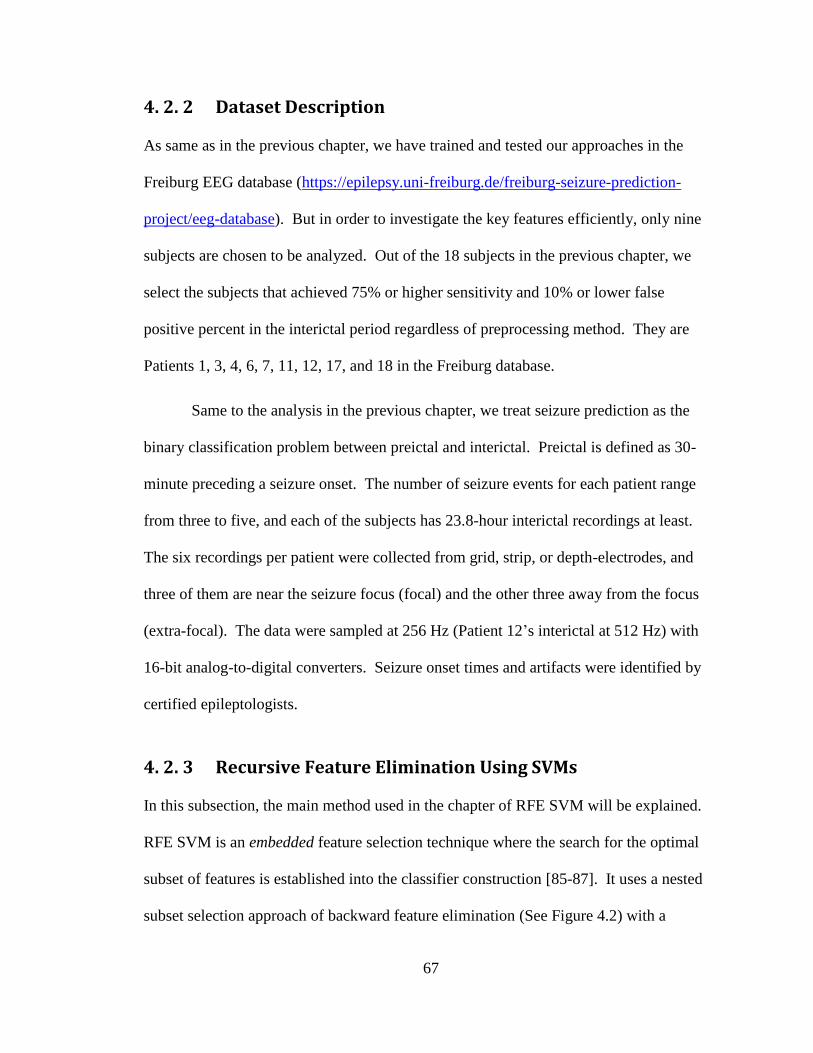
67

Dataset Description 4. 2. 2

As same as in the previous chapter, we have trained and tested our approaches in the

Freiburg EEG database (https://epilepsy.uni-freiburg.de/freiburg-seizure-prediction-

project/eeg-database). But in order to investigate the key features efficiently, only nine

subjects are chosen to be analyzed. Out of the 18 subjects in the previous chapter, we

select the subjects that achieved 75% or higher sensitivity and 10% or lower false

positive percent in the interictal period regardless of preprocessing method. They are

Patients 1, 3, 4, 6, 7, 11, 12, 17, and 18 in the Freiburg database.

Same to the analysis in the previous chapter, we treat seizure prediction as the

binary classification problem between preictal and interictal. Preictal is defined as 30-

minute preceding a seizure onset. The number of seizure events for each patient range

from three to five, and each of the subjects has 23.8-hour interictal recordings at least.

The six recordings per patient were collected from grid, strip, or depth-electrodes, and

three of them are near the seizure focus (focal) and the other three away from the focus

(extra-focal). The data were sampled at 256 Hz (Patient 12’s interictal at 512 Hz) with

16-bit analog-to-digital converters. Seizure onset times and artifacts were identified by

certified epileptologists.

Recursive Feature Elimination Using SVMs 4. 2. 3

In this subsection, the main method used in the chapter of RFE SVM will be explained.

RFE SVM is an embedded feature selection technique where the search for the optimal

subset of features is established into the classifier construction [85-87]. It uses a nested

subset selection approach of backward feature elimination (See Figure 4.2) with a

68

ranking criterion 2

iw , where w is the weighting vector in linear SVMs and i is the feature

number. The procedure is as follows:

(1) Initialization: the current subset of selected features x* is the set of all features x.

(2) Estimate a linear SVM model using the surviving features x*. Denote this linear

SVM model as f(x*, Copt), where the regularization parameter Copt is chosen so

that the SVM model with this parameter yields the minimum prediction risk

(misclassification rate) on an independent validation set (preferably through

cross-validation). Record the prediction risk R(x*).

(3) Calculate the ranking criterion 2

iw , rank the features x* by the criterion, and

eliminate the feature(s) with the smallest 2

iw .

(4) Repeat the above steps (2)-(4) until all features are eliminated.

(5) Choose the subset of features with which the SVM produced the smallest

misclassification rate R as the optimal subset of features xopt.

It is noted that the elimination criterion in RFE SVM is the smallest 2

iw . This

represents that the features to be eliminated are the ones that contribute least in forming

the margin of the linear SVM.

In general, feature selection techniques are categorized into three: filter, wrapper,

and embedded methods [86], and the RFE SVM analysis is into the embedded method.

RFE SVM, as the embedded method, has its excellent advantage that RFE SVM interacts

with the classifier of linear SVMs, and furthermore, the linear SVMs are used for both

the feature selection process and the subsequent classification. Thus, unlikely filter

techniques, where an optimal feature subset is investigated independent of the classifier

69

in the subsequent classification, RFE SVM may result in less discrepancies than filter

techniques. Also, RFE SVM is considered much less computationally intensive than the

wrapper method; in general, in the wrapper method, there are much more potentially

optimal subsets of features to be evaluated [86].

Feature Selection by RFE SVM for Reduced Complexity 4. 2. 4

Seizure Prediction

The key features for reducing the complexity of the initial seizure prediction algorithm

are investigated using a two-step RFE SVM method: coarse grained search with 9-feature

elimination per iteration and fine search with 3-feature elimination per iteration. The

coarse search begins with all 27-54 features, eliminates the least ranked 9 features per

iteration, and ends with the last 9 features. Then, the fine search begins with the top 18

features that survive in the last second elimination in the coarse grained search, removes

the least significant 3 features per iteration, and ends with the last surviving 3 features.

The detailed procedure is as follows:

Coarse grained search by 9-feature elimination per iteration

(1) Initialization: the coarse search begins with all 27-54 features x and sets the

surviving features x* as x.

(2) Estimate a linear cost-sensitive SVM model using the surviving features x*.

The linear SVM has a cost-sensitive factor of 8 so that the training errors on the

positive (preictal) samples outweigh those on the negative (interictal) samples

by 8. The regularization parameter Copt is chosen in the range of between 23 and

215

in the step of power of 2 and it produces the highest F2-measure among the

70

Cs. The F2-measure is calculated on independent validation sets by k-fold

cross-validation, where k is the number of preictal events that the subject has.

(3) Calculate the ranking criterion 2

iw , rank the features x* by the criterion, and

eliminate the 9 features with the smallest 2

iw .

(4) Repeat the above steps (2)-(4) until all features are eliminated.

The fine grained search with 3-feature elimination per iteration is similar as the coarse

grained search. But, it begins with the top 18 features that have survived in the last

second iteration of the coarse search, and 3 features with the least ranks are removed

rather than 9 features in the elimination step. The SVM-Light [88] has been used for the

feature selection and linear classification. It is noted that the original RFE SVM search

for a subset of features, which can produce the highest prediction rate (lowest predictor

error), no matter how many the features are used. However, we have used the RFE SVM

analysis to search for a small number of features, which can produce acceptable

sensitivity and specificity.

The features that have been investigated for feature selection are the same ones

that were used in the seizure prediction algorithm in the previous chapter. They are

spectral power in 9 bands of delta (0.5-4 Hz), theta (4-8 Hz), alpha (8-13 Hz), beta (13-30

Hz), and four gamma bands (30-47, 53-75, 75-97, and 103-128 Hz, excluding power line

hums at 50 and 100 Hz) and their total. The first eight spectral power features represent

relative power to the total power, where power in the specific band is normalized by the

power in the entire band except the power line hums. We have used the moving window

analysis: each of the feature sets is extracted in a 20-second long window that contains

71

10-second long updated EEG. This corresponds to a 50% overlap between two

consecutive windows.

In order to investigate the effect of preprocessing, four types of the spectral power

features have been investigated: raw, time-differential, bipolar, and bipolar/time-

differential preprocessed spectral power features (See Figure 4.3 and Figure 4.4). Raw

features are computed from the original iEEG without any preprocessing. Time-

differential preprocessing computes an approximate derivative in iEEG. Bipolar

preprocessing subtracts electrical potentials between the two channels that are within

focal, extra-focal, or physically neighbored. For example, in Figure 4.3, bipolar features

have been calculated from the iEEG between Electrodes 1 and 2, 3 and 6, and 4 and 5.

Bipolar/time-differential preprocessed EEG represents one that is preprocessed by both

bipolar and time-differential methods.

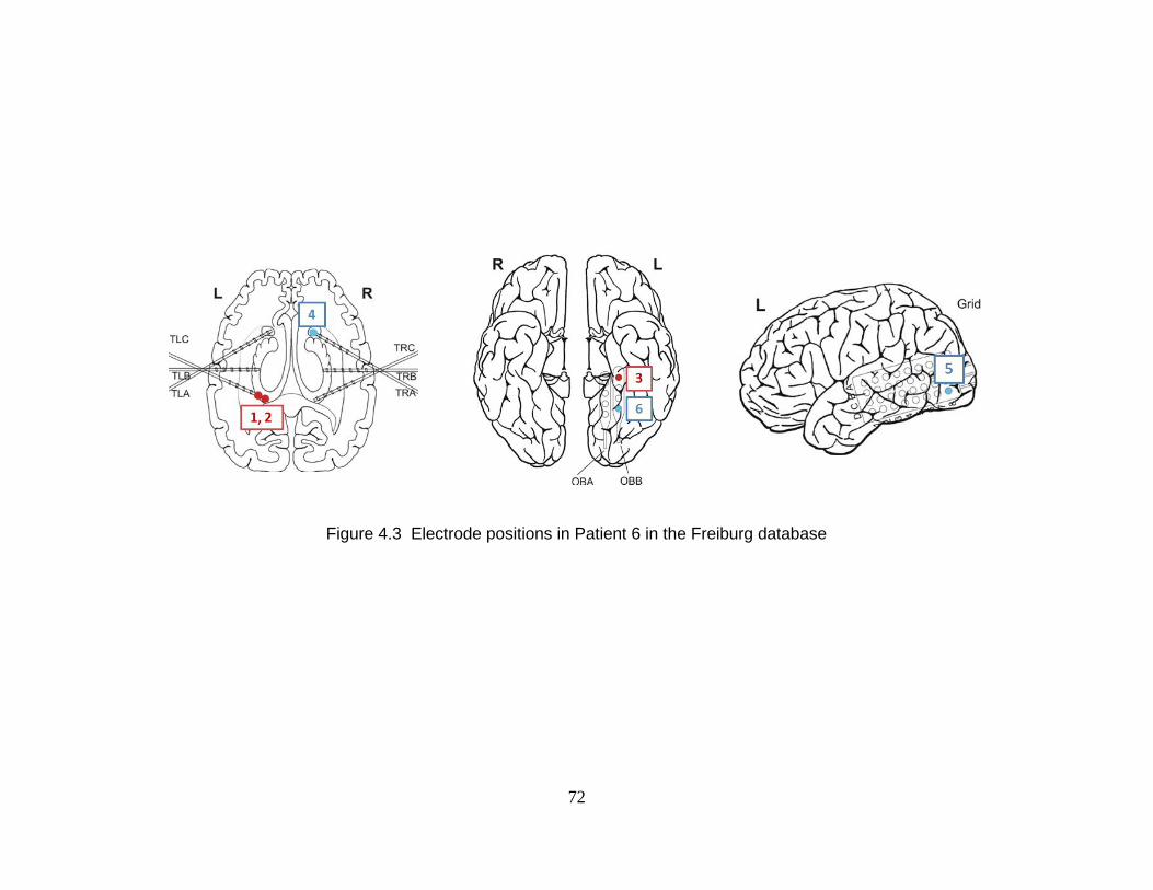
72

Figure 4.3 Electrode positions in Patient 6 in the Freiburg database

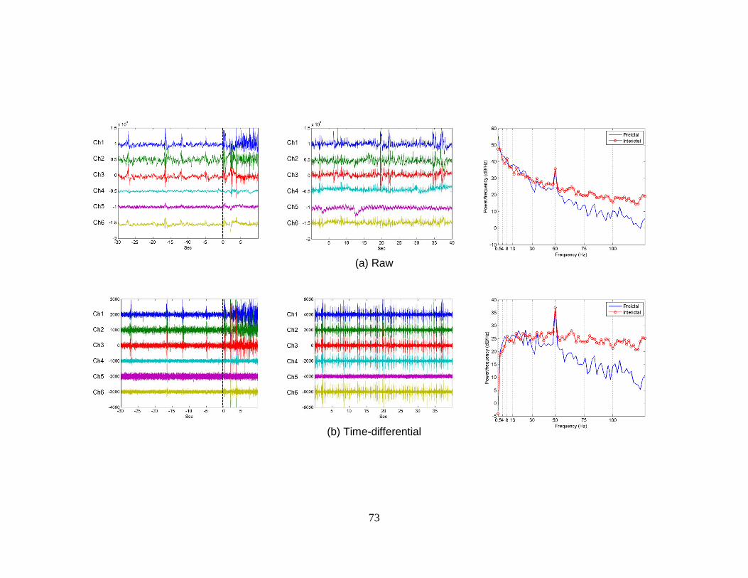
73

(a) Raw

(b) Time-differential

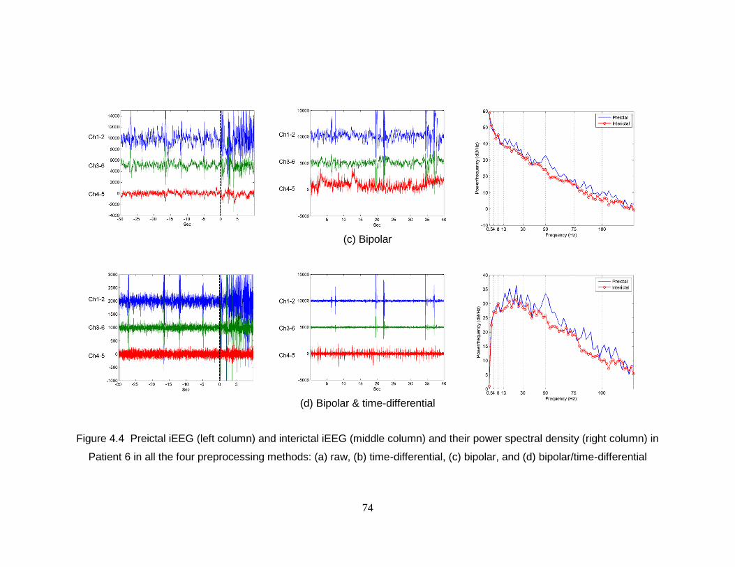
74

(c) Bipolar

(d) Bipolar & time-differential

Figure 4.4 Preictal iEEG (left column) and interictal iEEG (middle column) and their power spectral density (right column) in

Patient 6 in all the four preprocessing methods: (a) raw, (b) time-differential, (c) bipolar, and (d) bipolar/time-differential

75

Postprocessing by Kalman Filter or Moving-Average Filter 4. 2. 5

In the prior prediction algorithm, the Kalman filter was used to reduce the number of

jittering that causes a number of false positives. In this sub-chapter, we have tested

moving-average filters as well as the Kalman filter for postprocessing and have

investigated if the moving-average filter can replace the Kalman filter without loss of

high prediction rate.

In order to lower the complexity while maintaining high sensitivity and lower

false positive rate, several types of moving average filters have been investigated. These

include 5-tap, 10-tap, and 20-tap moving average filters. The proposed reduced-

complexity algorithm employs the 20-tap moving-average filter for postprocess. It is

noted that moving-average filters are expected to have lower complexity than the Kalman

filter in general, because moving-average filters can be implemented in hardware without

any multipliers while the Kalman filter requires matrix-multiplications. In addition, the

Kalman filter has been tested as well. It has been tested in order to directly compare

prediction rate that results from linear SVMs with small numbers of selected features,

which has been proposed in this chapter, with prediction rate that resulted from nonlinear

SVMs with all features in the previous chapter.

76

Results 4. 3

RFE SVM Results 4. 3. 1

We have investigated small numbers of key features by the two-step RFE SVM analysis,

and four different preprocessed features have been investigated. It has been tested on

iEEG of nine patients with 38 seizures and 217.5-hour interictal recordings in the

Freiburg database. The nine subjects have been selected based on the results in our prior

prediction work [5], which produced 75% or higher sensitivity and 10% or lower percent

of false positive proportion in interictal recordings.

A typical example of the result from the RFE SVM analysis is shown as

Figure 4.5, which corresponds to Patient 6 in the Freiburg database. It demonstrates how

F2-measure, sensitivity, and specificity vary, as the RFE SVM analysis progresses and a

certain number of features are eliminated. The coarse search starts with all the 27-54

features (depending on the preprocessing method) and eliminates 9 features per iteration.

Then, the fine search starts with the 18 features that survive as the top 18 features in the

coarse search, eliminates 3 features per iteration, and ends with the last 3 features. It is

noted that F2-measure has been used as a criterion for evaluating prediction rates in the

RFE SVM analysis and it is calculated based on the numbers of windows, not on the

numbers of seizure events.

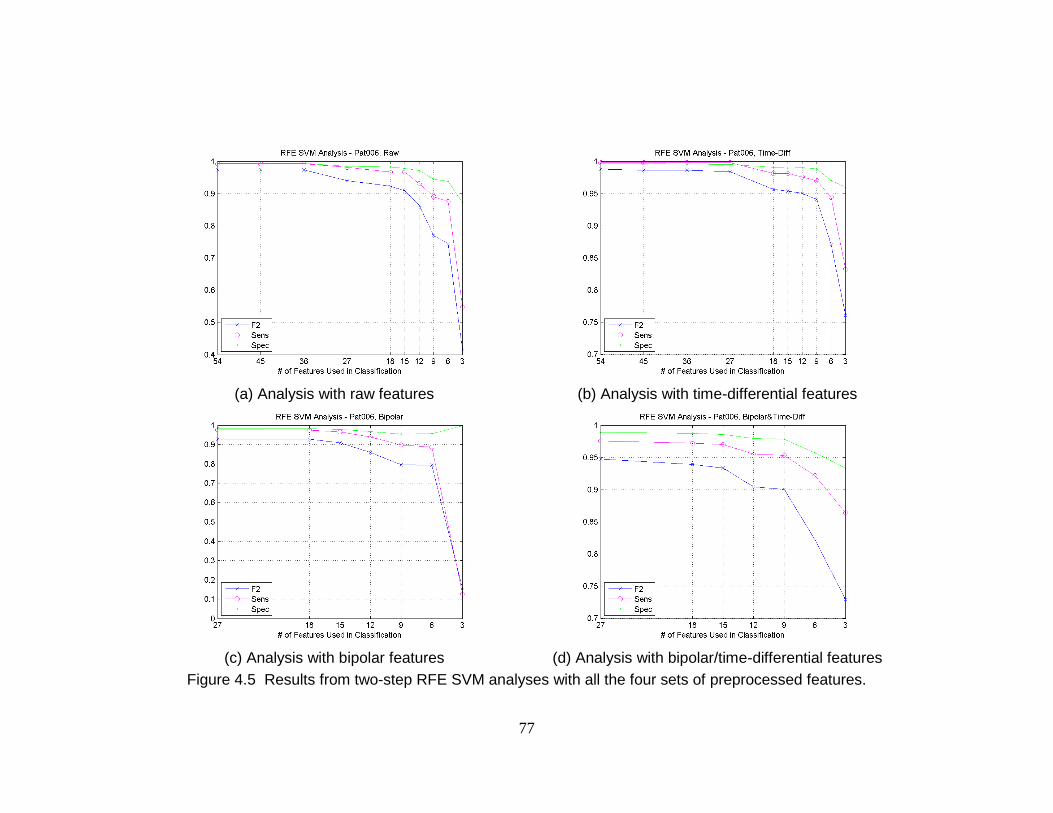
77

Figure 4.5 Results from two-step RFE SVM analyses with all the four sets of preprocessed features.

(a) Analysis with raw features

(b) Analysis with time-differential features

(c) Analysis with bipolar features

(d) Analysis with bipolar/time-differential features

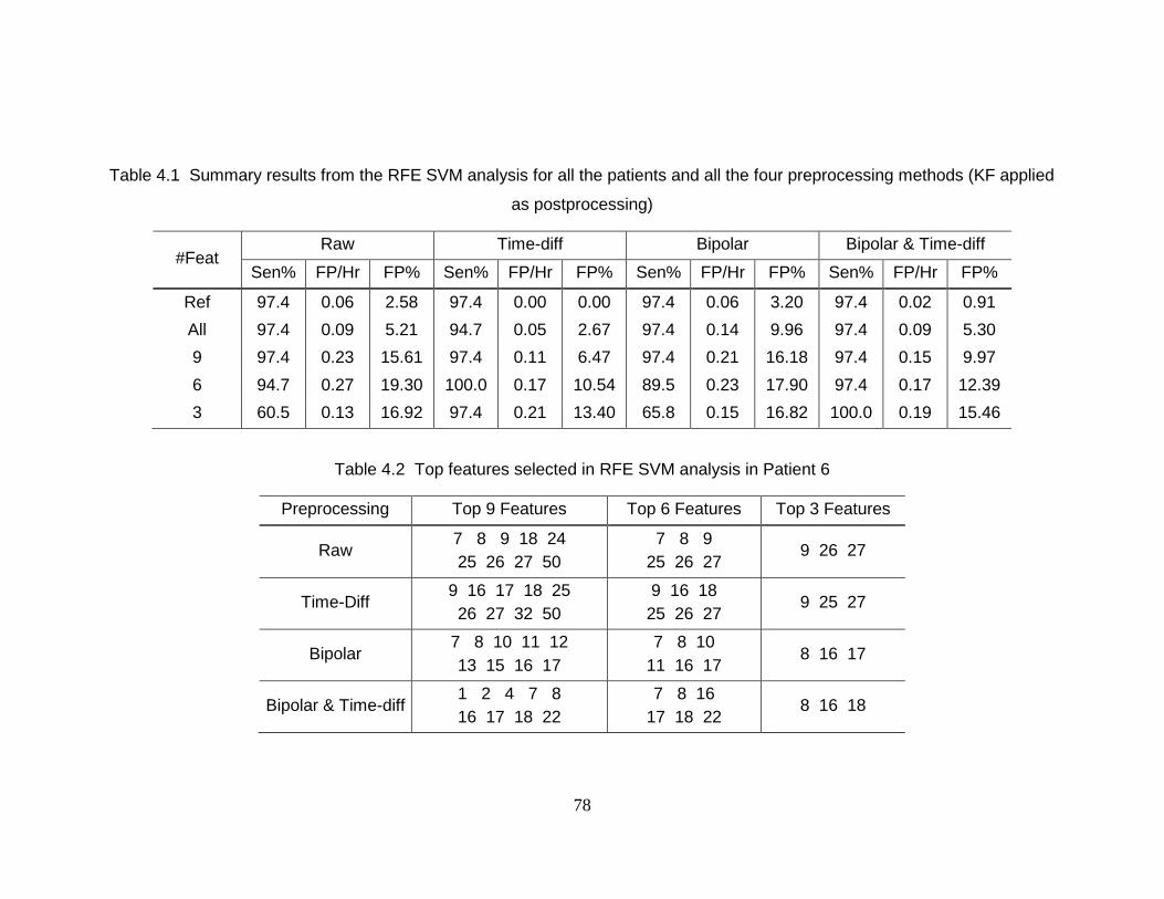
78

Table 4.1 Summary results from the RFE SVM analysis for all the patients and all the four preprocessing methods (KF applied

as postprocessing)

#Feat Raw Time-diff Bipolar Bipolar & Time-diff

Sen% FP/Hr FP% Sen% FP/Hr FP% Sen% FP/Hr FP% Sen% FP/Hr FP%

Ref 97.4 0.06 2.58 97.4 0.00 0.00 97.4 0.06 3.20 97.4 0.02 0.91

All 97.4 0.09 5.21 94.7 0.05 2.67 97.4 0.14 9.96 97.4 0.09 5.30

9 97.4 0.23 15.61 97.4 0.11 6.47 97.4 0.21 16.18 97.4 0.15 9.97

6 94.7 0.27 19.30 100.0 0.17 10.54 89.5 0.23 17.90 97.4 0.17 12.39

3 60.5 0.13 16.92 97.4 0.21 13.40 65.8 0.15 16.82 100.0 0.19 15.46

Table 4.2 Top features selected in RFE SVM analysis in Patient 6

Preprocessing Top 9 Features Top 6 Features Top 3 Features

Raw 7 8 9 18 24

25 26 27 50

7 8 9

25 26 27 9 26 27

Time-Diff 9 16 17 18 25

26 27 32 50

9 16 18

25 26 27 9 25 27

Bipolar 7 8 10 11 12

13 15 16 17

7 8 10

11 16 17 8 16 17

Bipolar & Time-diff 1 2 4 7 8

16 17 18 22

7 8 16

17 18 22 8 16 18

79

As illustrated in Figure 4.5, as the number of features decreases, the prediction

rate deteriorates in general. Furthermore, it has been observed that the phenomenon of

the significant decline in prediction rate in nine to three features is somehow common.

To investigate it in more detail, we have applied linear SVMs as classification, the

Kalman filter as postprocessing, the 30-min prediction horizon criterion to all the nine

patients and all the preprocessing features, and the summary results are shown in Table

4.1.

Summary results from linear SVM classification and Kalman filtering with certain

numbers of key features for all the nine patients and all the four preprocessed features are

presented in Table 4.1. As a reference, the results from nonlinear SVM classification

with all the 27-54 features for all the selected nine patients are presented in the top row:

sensitivity of 97.4% (37/38) and false positive rate of 0.06 per hour (12 false positives)

and false positive percent of 2.58 (5.62-hour) in 217.5-hour interictal recordings with raw

iEEG. Compared to the nonlinear SVM classification, linear SVM classification with all

the 27-54 features generally demonstrates little deterioration in sensitivity but minor

degradation in false positive rate and percentage: in raw iEEG, sensitivity of 97.4%

(37/38) remains the same but the number of false positives increases (0.09/hour, 19 FPs)

as well as its portion in the interictal recordings (5.21%, 11.33-hour). It is noted that to

directly compare to the reference results, where the Kalman filter was used as

postprocessing, the results from linear SVM classification are postprocessed by the

Kalman filter as well.

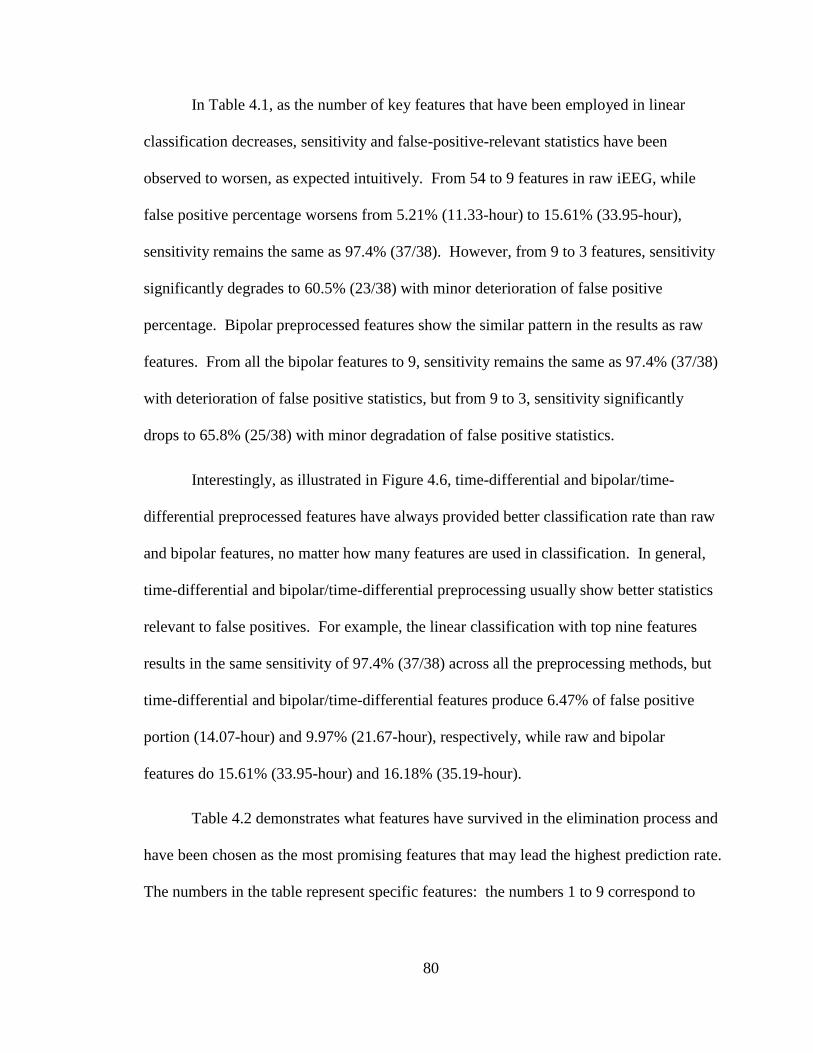
80

In Table 4.1, as the number of key features that have been employed in linear

classification decreases, sensitivity and false-positive-relevant statistics have been

observed to worsen, as expected intuitively. From 54 to 9 features in raw iEEG, while

false positive percentage worsens from 5.21% (11.33-hour) to 15.61% (33.95-hour),

sensitivity remains the same as 97.4% (37/38). However, from 9 to 3 features, sensitivity

significantly degrades to 60.5% (23/38) with minor deterioration of false positive

percentage. Bipolar preprocessed features show the similar pattern in the results as raw

features. From all the bipolar features to 9, sensitivity remains the same as 97.4% (37/38)

with deterioration of false positive statistics, but from 9 to 3, sensitivity significantly

drops to 65.8% (25/38) with minor degradation of false positive statistics.

Interestingly, as illustrated in Figure 4.6, time-differential and bipolar/time-

differential preprocessed features have always provided better classification rate than raw

and bipolar features, no matter how many features are used in classification. In general,

time-differential and bipolar/time-differential preprocessing usually show better statistics

relevant to false positives. For example, the linear classification with top nine features

results in the same sensitivity of 97.4% (37/38) across all the preprocessing methods, but

time-differential and bipolar/time-differential features produce 6.47% of false positive

portion (14.07-hour) and 9.97% (21.67-hour), respectively, while raw and bipolar

features do 15.61% (33.95-hour) and 16.18% (35.19-hour).

Table 4.2 demonstrates what features have survived in the elimination process and

have been chosen as the most promising features that may lead the highest prediction rate.

The numbers in the table represent specific features: the numbers 1 to 9 correspond to

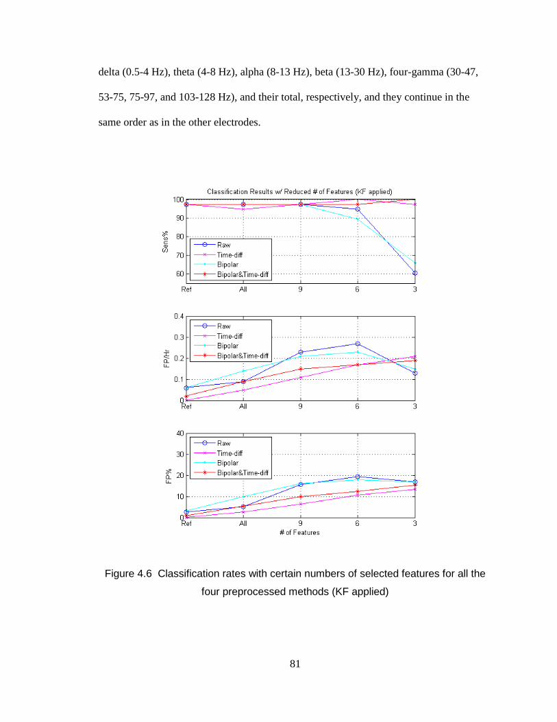
81

delta (0.5-4 Hz), theta (4-8 Hz), alpha (8-13 Hz), beta (13-30 Hz), four-gamma (30-47,

53-75, 75-97, and 103-128 Hz), and their total, respectively, and they continue in the

same order as in the other electrodes.

Figure 4.6 Classification rates with certain numbers of selected features for all the

four preprocessed methods (KF applied)

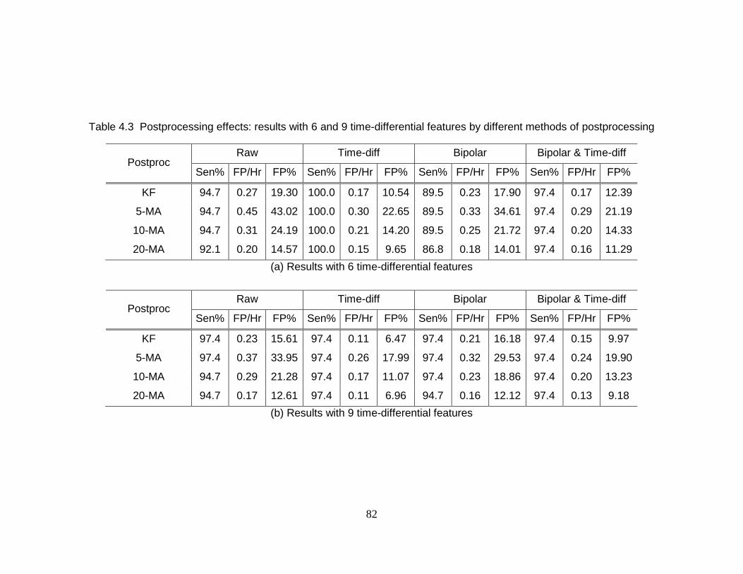
82

Table 4.3 Postprocessing effects: results with 6 and 9 time-differential features by different methods of postprocessing

Postproc Raw Time-diff Bipolar Bipolar & Time-diff

Sen% FP/Hr FP% Sen% FP/Hr FP% Sen% FP/Hr FP% Sen% FP/Hr FP%

KF 94.7 0.27 19.30 100.0 0.17 10.54 89.5 0.23 17.90 97.4 0.17 12.39

5-MA 94.7 0.45 43.02 100.0 0.30 22.65 89.5 0.33 34.61 97.4 0.29 21.19

10-MA 94.7 0.31 24.19 100.0 0.21 14.20 89.5 0.25 21.72 97.4 0.20 14.33

20-MA 92.1 0.20 14.57 100.0 0.15 9.65 86.8 0.18 14.01 97.4 0.16 11.29

(a) Results with 6 time-differential features

Postproc Raw Time-diff Bipolar Bipolar & Time-diff

Sen% FP/Hr FP% Sen% FP/Hr FP% Sen% FP/Hr FP% Sen% FP/Hr FP%

KF 97.4 0.23 15.61 97.4 0.11 6.47 97.4 0.21 16.18 97.4 0.15 9.97

5-MA 97.4 0.37 33.95 97.4 0.26 17.99 97.4 0.32 29.53 97.4 0.24 19.90

10-MA 94.7 0.29 21.28 97.4 0.17 11.07 97.4 0.23 18.86 97.4 0.20 13.23

20-MA 94.7 0.17 12.61 97.4 0.11 6.96 94.7 0.16 12.12 97.4 0.13 9.18

(b) Results with 9 time-differential features

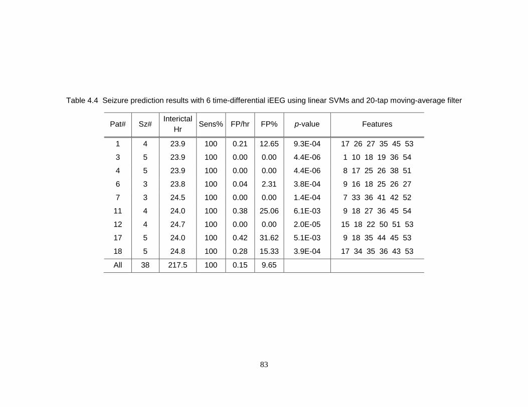
83

Table 4.4 Seizure prediction results with 6 time-differential iEEG using linear SVMs and 20-tap moving-average filter

Pat# Sz# Interictal

Hr Sens% FP/hr FP% p-value Features

1 4 23.9 100 0.21 12.65 9.3E-04 17 26 27 35 45 53

3 5 23.9 100 0.00 0.00 4.4E-06 1 10 18 19 36 54

4 5 23.9 100 0.00 0.00 4.4E-06 8 17 25 26 38 51

6 3 23.8 100 0.04 2.31 3.8E-04 9 16 18 25 26 27

7 3 24.5 100 0.00 0.00 1.4E-04 7 33 36 41 42 52

11 4 24.0 100 0.38 25.06 6.1E-03 9 18 27 36 45 54

12 4 24.7 100 0.00 0.00 2.0E-05 15 18 22 50 51 53

17 5 24.0 100 0.42 31.62 5.1E-03 9 18 35 44 45 53

18 5 24.8 100 0.28 15.33 3.9E-04 17 34 35 36 43 53

All 38 217.5 100 0.15 9.65

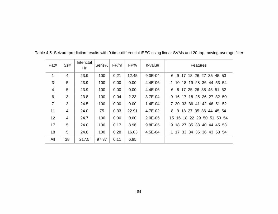
84

Table 4.5 Seizure prediction results with 9 time-differential iEEG using linear SVMs and 20-tap moving-average filter

Pat# Sz# Interictal

Hr Sens% FP/hr FP% p-value Features

1 4 23.9 100 0.21 12.45 9.0E-04 6 9 17 18 26 27 35 45 53

3 5 23.9 100 0.00 0.00 4.4E-06 1 10 18 19 28 36 44 53 54

4 5 23.9 100 0.00 0.00 4.4E-06 6 8 17 25 26 38 45 51 52

6 3 23.8 100 0.04 2.23 3.7E-04 9 16 17 18 25 26 27 32 50

7 3 24.5 100 0.00 0.00 1.4E-04 7 30 33 36 41 42 46 51 52

11 4 24.0 75 0.33 22.91 4.7E-02 8 9 18 27 35 36 44 45 54

12 4 24.7 100 0.00 0.00 2.0E-05 15 16 18 22 29 50 51 53 54

17 5 24.0 100 0.17 8.96 9.8E-05 9 18 27 35 38 40 44 45 53

18 5 24.8 100 0.28 16.03 4.5E-04 1 17 33 34 35 36 43 53 54

All 38 217.5 97.37 0.11 6.95

85

Since we employ linear features and simple classifiers of linear SVMs for

enhancing implantable capabilities, we have examined other simple postprocessing

strategies other than the Kalman filter that can also improve “implant-abilities”: 5-point,

10-point, and 20-point moving-average filters (See Figure 4.7 and Table 4.3). In general,

the results from 5-tap and 10-tap moving-average filters are not better than the ones from

the Kalman filter. However, when it comes up to the 20-tap moving average filter, it

starts to outperform the Kalman filter with respect to the prediction rate. Furthermore,

when the postprocessing system’s complexity as well as the prediction rate is considered,

the 20-tap moving-average filter outperforms the Kalman filter, because the moving-

average filter can be built in hardware just with adders but the Kalman filter

implementation in hardware require several multipliers, whose complexity is much

higher than that of the adders.

Summary results with top 6 and 9 time-differential features of iEEG using linear

SVMs and the 20-tap moving-average filter for all the nine subjects are presented in

Table 4.4 and Table 4.5, respectively. In the tables, we have presented sensitivity and

false positive rate and false positive percentage in interictal recordings. Furthermore, we

have tested those results against the null hypothesis that comes with a chance predictor by

estimating one-sided p-values [5, 69]. Based on the estimated p-values in Table 4.4 and

Table 4.5, our prediction algorithm with top 6 and 9 time-differential iEEG performs

significantly better than chance at a significance cutoff of 0.05.

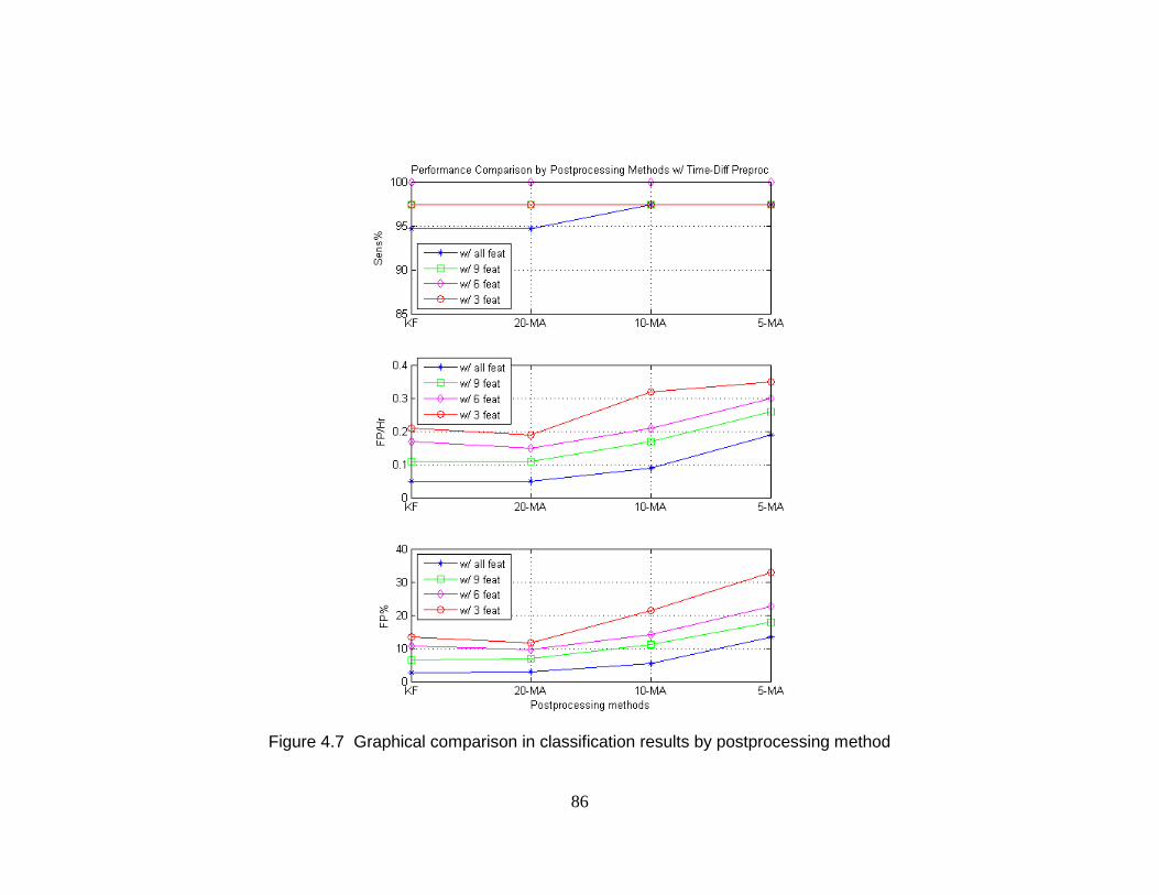
86

Figure 4.7 Graphical comparison in classification results by postprocessing method

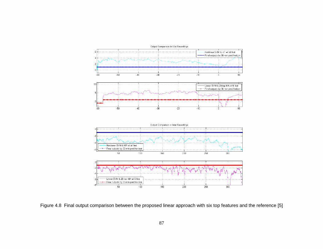
87

Figure 4.8 Final output comparison between the proposed linear approach with six top features and the reference [5]

88

Discussions 4. 4

The proposed approach for seizure prediction with iEEG has reduced the algorithm’s

complexity, while maintaining its high prediction rate. This approach has been tested

with the nine patients’ iEEG from the Freiburg using cross-validation for in-sample

optimization and out-of-sample testing [1, 5]. Our approach, which uses the linear SVM

and 20-tap moving average filter with the selected six time-differential features, has

successfully demonstrated high sensitivity of 100.0% (38/38) as well as low false positive

rate of 0.15 per hour (32 FPs) and false positive portion of 9.65% (21.0-hour) in the

217.5-hour interictal recordings.

In our prior work [9, 10, 89], we proposed a seizure prediction algorithm that can

produce high prediction rate using only linear features of spectral power of iEEG.

However, the algorithm’s complexity may be too high to be used in an implantable

device, because it uses 27-54 features, nonlinear SVMs for classification, and the Kalman

filter for postprocessing. In this chapter, we have lowered the algorithm’s complexity by

the following three approaches: investigating and using the key features, substituting

nonlinear SVMs with linear SVMs, and replacing the Kalman filter with the moving-

average filter. Using only the essential features in classification represents that the

system does not need to extract and calculate many other insignificant features. Thus, the

system can be less complex and consume less power for feature extraction. Also, as

demonstrated in [56], replacing nonlinear SVMs with linear SVMs in an actual device

can significantly lower in the system’s complexity and the power consumption of the

89

device. Furthermore, the moving-average filter is much less complex than the Kalman

filter. The two-tap Kalman filter in [5] requires five multipliers and 24 adders, whereas

the 20-tap moving-average filter just requires 19 adders.

An important aspect in key feature investigation in raw, time-differential, bipolar,

and bipolar/time-differential iEEG is that time-differential preprocessing has been

observed to improve the prediction rate significantly. In our prior work [5], when all 27-

54 features were used, we observed that time-differential preprocessing can reduce false

positives in seizure prediction. Furthermore, in this chapter, we have also observed that

the time-differential preprocessing with a few selected features can significantly lower

false positive rates and its portions in interictal recordings, while maintaining high

sensitivity. For example, in classification with top 9 features, time-differential

preprocessing lowered 52.2% of false positive rates (0.23 FP/hr in raw iEEG to 0.11

FP/hr in time-differential iEEG) and 58.6% of false positive portions in interictal

recordings (15.61% to 6.47%). Similarly, the effect of time-differential preprocessing in

reducing false positives have been observed in bipolar/time-differential preprocessing,

where the time-differential method was applied to bipolar iEEG. However, bipolar

preprocessing has not demonstrated any significant improvements in the prediction rate.

Also, from the key feature investigation in the RFE SVM analysis, we have

observed that all the 27-54 features are not necessary to produce high sensitivity and low

false positive rates: only six or nine key features are enough to make the excellent

prediction rate. Having all the 54 time-differential features, the linear classifiers with the

Kalman filter have produced sensitivity of 94.7% (36/38) and 0.05 FP/hr (11 FPs) in the

90

interictal recordings. With only six or nine time-differentially preprocessed features, they

have successfully generated sensitivity of 100% (38/38) and 0.17 FP/hr (37 FPs) or

sensitivity of 97.4% (37/38) and 0.11 FP/hr (24 FPs). It is noted that the higher

sensitivity with smaller numbers of features may be explained as compensation for

decrease in false positive statistics.

The RFE SVM analysis is generally used for analyzing a subset of features that

may produce the highest prediction rate, but we have used the method to investigate a

small number of top features that may lead to acceptable prediction rate. Our approach

considers practical situations, where a device’s power consumption is limited, i.e., the

number of features is bounded.

Though we have investigated key features and have achieved successful

prediction rate with them, the criterion for deciding the best number of key features still

remains uncertain. For example, we urge that six or nine key features produce high

prediction rate and reduce the system’s complexity, but we may not decide which are

better clearly. The criterion for choosing the best number of key features may optimally

compromise between prediction rate and the system’s complexity.

For evaluating seizure prediction algorithms, Mormann et al. suggested to use the

three measures: sensitivity and false positive rate and its portion in interictal recordings

[5]. However, from the practical engineering perspective, those three scientific numbers

are not sufficient, because they do not account for practical engineering issues. For

example, even if certain nonlinear measures are very successful indicators for seizure

prediction, it would be very difficult to make a practical device that employs the

91

nonlinear features, due to the impractical computational complexity of the feature

extraction. Our features of spectral power in multiple bands are simpler and more

practical: they can be calculated by using several filter banks and squaring the amplitudes

in time-domain or can be further approximately estimated by using wavelets.

Our spectral power features are feasible in practical engineering sense, but the set

of key features are extracted from multi-electrodes. The average number of the

electrodes used for extraction of the six time-differential key features in all the nine

subjects is 4.44 ± 1.01, and that for the nine time-differential key features is 5.22 ± 0.83.

Also, those six or nine features were extracted almost equally from focal and extra-focal

electrodes. Scientifically, this observation may be interesting, because it demonstrates

that the features from extra-focal areas are as significant as those from focal areas for

seizure prediction. However, from the engineering perspective, the fact that multi-

electrode key features are necessary may be undesirable, because the device that uses our

seizure prediction approach needs to use multi-electrodes to produce our high sensitivity

and low false positive rate.

We have used F2-measure to represent both sensitivity and specificity as a single

criterion in the binary classification of preictal and interictal in the RFE SVM analysis.

Sensitivity and specificity, or sensitivity, false positive rate, and the percentage of false

positives are generally accepted measures to evaluate the prediction algorithms [1].

However, they do not measure a single quantity. In many cases, a single quantity is

necessary to figure out the best prediction model, such as in the analysis using RFE SVM.

F2-measure, which had been proposed in our prior work as a single measure for seizure

92

prediction evaluation, has successfully represented a model’s prediction rate as a single

number in the RFE SVM analysis. It is noted that F2-measure does not cover true

negatives; the Matthews correlation coefficient [90] can be an effective alternative to F2-

measure when true negatives need to be counted.

Conclusion 4. 5

We have proposed a reduce-complexity seizure prediction approach that uses a small

number of linear features of spectral power of iEEG, linear classifiers of SVMs, and a

less complex postprocessing filter of moving-average. To investigate a small number of

key features, we have used RFE SVM, which is a feature selection method using

backward feature elimination. By applying RFE SVM to raw, time-differential, bipolar,

and bipolar/time-differential iEEG, we have observed that time-differential preprocessing

significantly improves the rate of prediction with small numbers of features. We have

further reduced the seizure prediction system’s complexity by substituting the Kalman

filter of the prior system with moving-average filters. With a small number of linear

features, linear classifiers, and a simple moving-average postprocessing filter, the

proposed algorithm has improved the feasibility of implantable devices for seizure

prediction.

93

Chapter 5

Enhanced Seizure Detection System with

Rat’s ECoG

Introduction 5. 1

In the previous two chapters we developed a seizure prediction algorithm. In this chapter,

we will investigate a seizure detection algorithm to be used in seizure termination

experiments with rats. Investigating rats’ brain is advantages to understand seizure

evolution, because it is much less complex than human. Specifically, when it comes to

how seizures evolve in human brains, complex human brain physiology prevents seizures

from being understood. To understand seizure evolution or test noble anti-seizure-

relevant approaches in simpler brains than human ones, researchers have used rats’ [91-

94].

In [15-17], Yang et al. proposed an automatic seizure detection system with rats’

ECoG for testing their experimental seizure termination approaches by focal cooling [15,

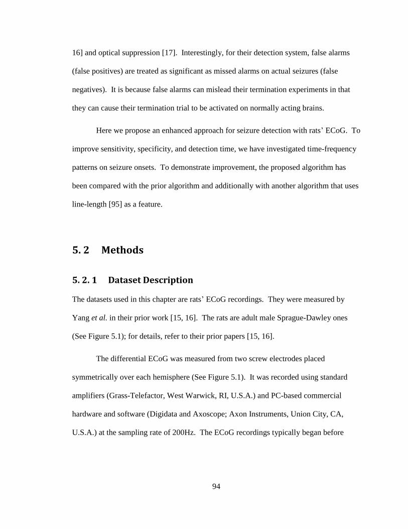
94

16] and optical suppression [17]. Interestingly, for their detection system, false alarms

(false positives) are treated as significant as missed alarms on actual seizures (false

negatives). It is because false alarms can mislead their termination experiments in that

they can cause their termination trial to be activated on normally acting brains.

Here we propose an enhanced approach for seizure detection with rats’ ECoG. To

improve sensitivity, specificity, and detection time, we have investigated time-frequency

patterns on seizure onsets. To demonstrate improvement, the proposed algorithm has

been compared with the prior algorithm and additionally with another algorithm that uses

line-length [95] as a feature.

Methods 5. 2

Dataset Description 5. 2. 1

The datasets used in this chapter are rats’ ECoG recordings. They were measured by

Yang et al. in their prior work [15, 16]. The rats are adult male Sprague-Dawley ones

(See Figure 5.1); for details, refer to their prior papers [15, 16].

The differential ECoG was measured from two screw electrodes placed

symmetrically over each hemisphere (See Figure 5.1). It was recorded using standard

amplifiers (Grass-Telefactor, West Warwick, RI, U.S.A.) and PC-based commercial

hardware and software (Digidata and Axoscope; Axon Instruments, Union City, CA,

U.S.A.) at the sampling rate of 200Hz. The ECoG recordings typically began before

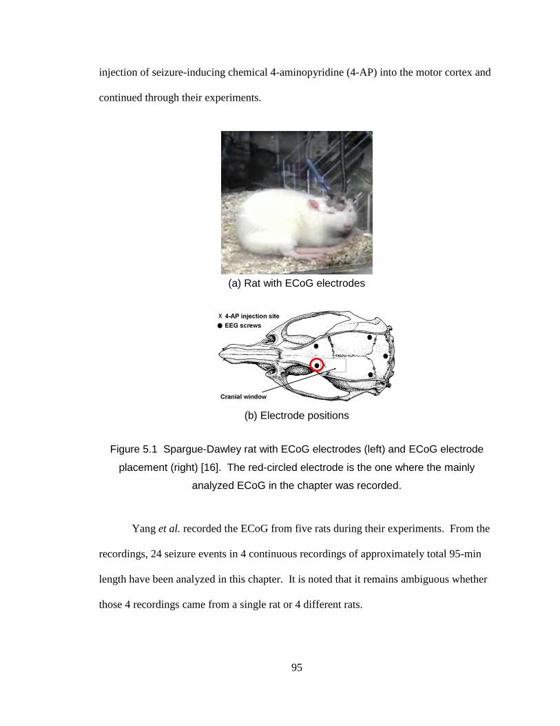
95

injection of seizure-inducing chemical 4-aminopyridine (4-AP) into the motor cortex and

continued through their experiments.

(a) Rat with ECoG electrodes

(b) Electrode positions

Figure 5.1 Spargue-Dawley rat with ECoG electrodes (left) and ECoG electrode

placement (right) [16]. The red-circled electrode is the one where the mainly

analyzed ECoG in the chapter was recorded.

Yang et al. recorded the ECoG from five rats during their experiments. From the

recordings, 24 seizure events in 4 continuous recordings of approximately total 95-min

length have been analyzed in this chapter. It is noted that it remains ambiguous whether

those 4 recordings came from a single rat or 4 different rats.

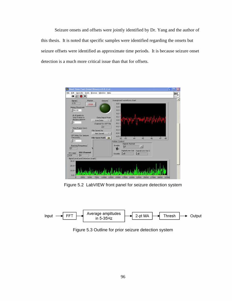
96

Seizure onsets and offsets were jointly identified by Dr. Yang and the author of

this thesis. It is noted that specific samples were identified regarding the onsets but

seizure offsets were identified as approximate time periods. It is because seizure onset

detection is a much more critical issue than that for offsets.

Figure 5.2 LabVIEW front panel for seizure detection system

Figure 5.3 Outline for prior seizure detection system

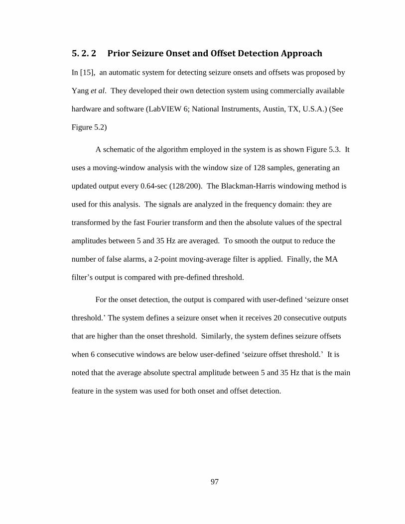
97

Prior Seizure Onset and Offset Detection Approach 5. 2. 2

In [15], an automatic system for detecting seizure onsets and offsets was proposed by

Yang et al. They developed their own detection system using commercially available

hardware and software (LabVIEW 6; National Instruments, Austin, TX, U.S.A.) (See

Figure 5.2)

A schematic of the algorithm employed in the system is as shown Figure 5.3. It

uses a moving-window analysis with the window size of 128 samples, generating an

updated output every 0.64-sec (128/200). The Blackman-Harris windowing method is

used for this analysis. The signals are analyzed in the frequency domain: they are

transformed by the fast Fourier transform and then the absolute values of the spectral

amplitudes between 5 and 35 Hz are averaged. To smooth the output to reduce the

number of false alarms, a 2-point moving-average filter is applied. Finally, the MA

filter’s output is compared with pre-defined threshold.

For the onset detection, the output is compared with user-defined ‘seizure onset

threshold.’ The system defines a seizure onset when it receives 20 consecutive outputs

that are higher than the onset threshold. Similarly, the system defines seizure offsets

when 6 consecutive windows are below user-defined ‘seizure offset threshold.’ It is

noted that the average absolute spectral amplitude between 5 and 35 Hz that is the main

feature in the system was used for both onset and offset detection.

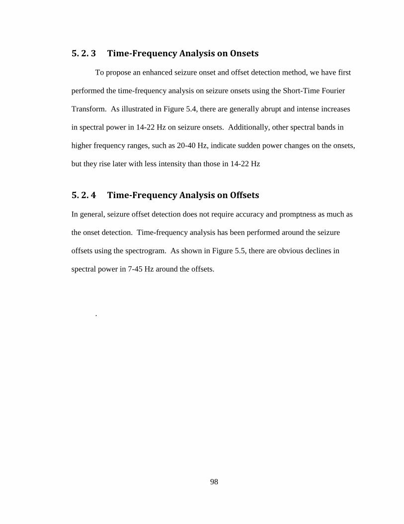
98

Time-Frequency Analysis on Onsets 5. 2. 3

To propose an enhanced seizure onset and offset detection method, we have first

performed the time-frequency analysis on seizure onsets using the Short-Time Fourier

Transform. As illustrated in Figure 5.4, there are generally abrupt and intense increases

in spectral power in 14-22 Hz on seizure onsets. Additionally, other spectral bands in

higher frequency ranges, such as 20-40 Hz, indicate sudden power changes on the onsets,

but they rise later with less intensity than those in 14-22 Hz

Time-Frequency Analysis on Offsets 5. 2. 4

In general, seizure offset detection does not require accuracy and promptness as much as

the onset detection. Time-frequency analysis has been performed around the seizure

offsets using the spectrogram. As shown in Figure 5.5, there are obvious declines in

spectral power in 7-45 Hz around the offsets.

.

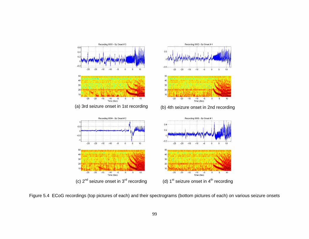
99

(a) 3rd seizure onset in 1st recording

(b) 4th seizure onset in 2nd recording

(c) 2

nd seizure onset in 3

rd recording

(d) 1

st seizure onset in 4

th recording

Figure 5.4 ECoG recordings (top pictures of each) and their spectrograms (bottom pictures of each) on various seizure onsets

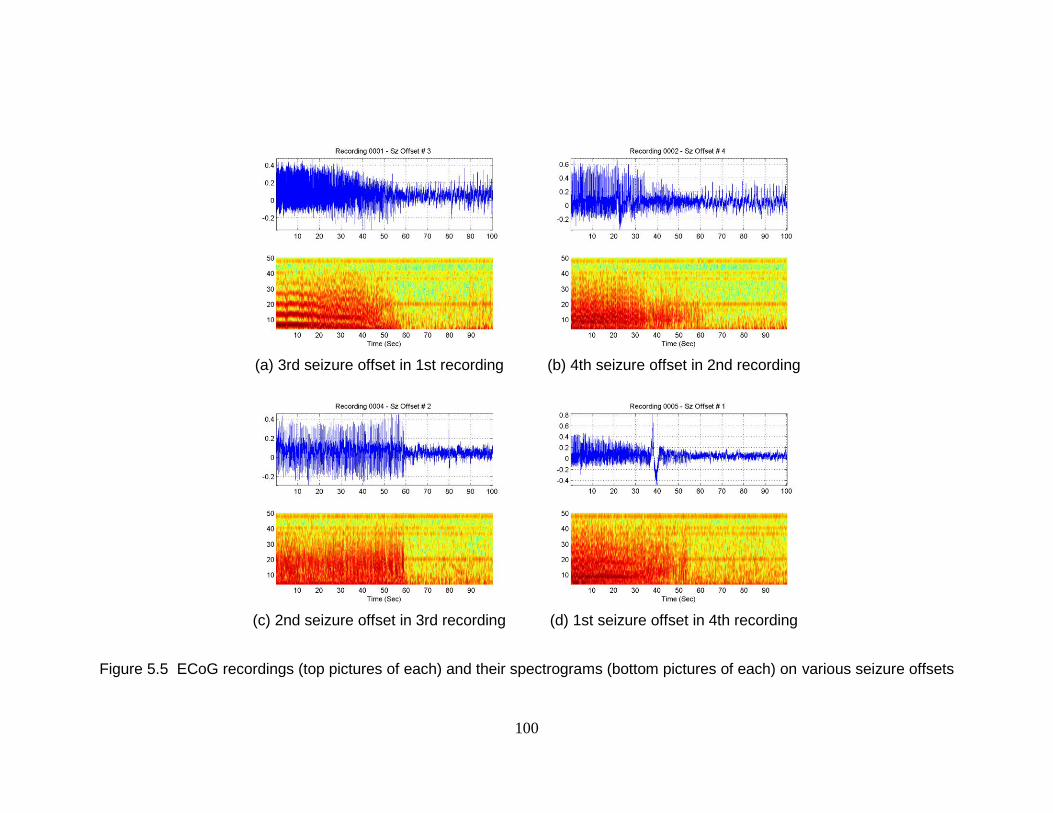
100

(a) 3rd seizure offset in 1st recording

(b) 4th seizure offset in 2nd recording

(c) 2nd seizure offset in 3rd recording

(d) 1st seizure offset in 4th recording

Figure 5.5 ECoG recordings (top pictures of each) and their spectrograms (bottom pictures of each) on various seizure offsets

101

Proposed Seizure Onset and Offset Detection Approach 5. 2. 5

Based on the time-frequency analyses on the onsets and offsets, we propose an enhanced

approach for onset and offset detection. The outline of our proposed algorithm is

illustrated in Figure 5.6.

(a) Proposed seizure onset detection algorithm

(b) Proposed seizure offset detection algorithm

Figure 5.6 Proposed algorithm for seizure onset and offset detection

Over their prior algorithm, the proposed algorithm has been improved as follows.

First, two different spectral power features are used for onset and offset detection but in

the same structure of the algorithm. We use spectral power in 14-22 Hz for onset

detection and that in 7-35 Hz for offset detection, but they differ only in the frequency

band. Second, rather than spectral amplitudes, the proposed algorithm uses spectral

power. The spectral power is achieved by squaring corresponding amplitudes and can

indicate seizure onsets more clearly than the amplitudes. Lastly, the Kalman filter is used

for postprocessing. The Kalman filter is expected to dampen sudden changes of spectral

power and thus produce more smooth outputs than the 2-point moving average filter.

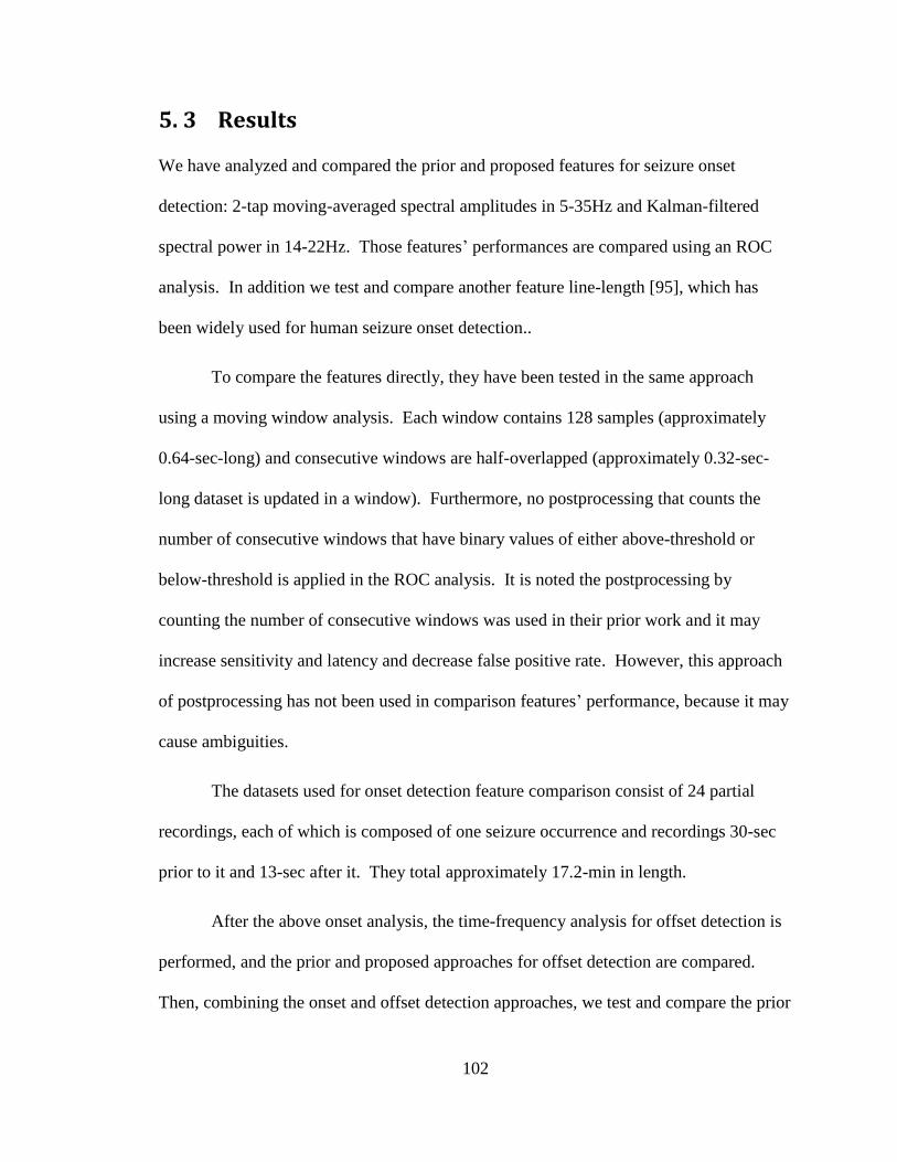
102

Results 5. 3

We have analyzed and compared the prior and proposed features for seizure onset

detection: 2-tap moving-averaged spectral amplitudes in 5-35Hz and Kalman-filtered

spectral power in 14-22Hz. Those features’ performances are compared using an ROC

analysis. In addition we test and compare another feature line-length [95], which has

been widely used for human seizure onset detection..

To compare the features directly, they have been tested in the same approach

using a moving window analysis. Each window contains 128 samples (approximately

0.64-sec-long) and consecutive windows are half-overlapped (approximately 0.32-sec-

long dataset is updated in a window). Furthermore, no postprocessing that counts the

number of consecutive windows that have binary values of either above-threshold or

below-threshold is applied in the ROC analysis. It is noted the postprocessing by

counting the number of consecutive windows was used in their prior work and it may

increase sensitivity and latency and decrease false positive rate. However, this approach

of postprocessing has not been used in comparison features’ performance, because it may

cause ambiguities.

The datasets used for onset detection feature comparison consist of 24 partial

recordings, each of which is composed of one seizure occurrence and recordings 30-sec

prior to it and 13-sec after it. They total approximately 17.2-min in length.

After the above onset analysis, the time-frequency analysis for offset detection is

performed, and the prior and proposed approaches for offset detection are compared.

Then, combining the onset and offset detection approaches, we test and compare the prior

103

and proposed algorithms. Finally, we test the proposed algorithm in one continuous

ECoG recording.

Prior Approach for Onset Detection Using Spectral 5. 3. 1

Amplitudes in 5-35Hz and 2-point Moving-Average Filter

The feature used in the prior approach is spectral amplitudes in 5-35Hz that are averaged

in a window of 128 samples and subsequently are smoothed by the 2-tap moving-

averaging filter with a feature in the previous window. Figure 5.7 demonstrates the

spectral amplitudes in 5-35Hz in cyan and their 2-tap moving-averaged ones in blue. The

corresponding states of either preictal or ictal are illustrated in red: low for preictal and

high for ictal. The features demonstrated in Figure 5.7 are the ones concatenated in 24

continuous recordings, each of which contains a seizure event.

We have performed the ROC analysis on the 2-tap moving-averaged features and

the result is shown in Figure 5.8. To achieve the ROC curve, 100 threshold values that

are equally allocated between the maximum and minimum of the values of features are

used. Also, to compare the performance with other features’, the area under the curve

(AUC) has been calculated. The AUC with the features of the 2-tap moving-averaged

spectral amplitudes is 0.9476. It is noted that the ROC and AUC analyses in this chapter

are based on the number of windows, not on the number of seizure events.

104

Figure 5.7 Prior algorithm’s features (spectral amplitudes in 5-35Hz and their 2-pt MA-filtered values) on seizure onsets

Figure 5.8 ROC analysis in 2-pt MA-filtered spectral amplitudes in 5-35Hz

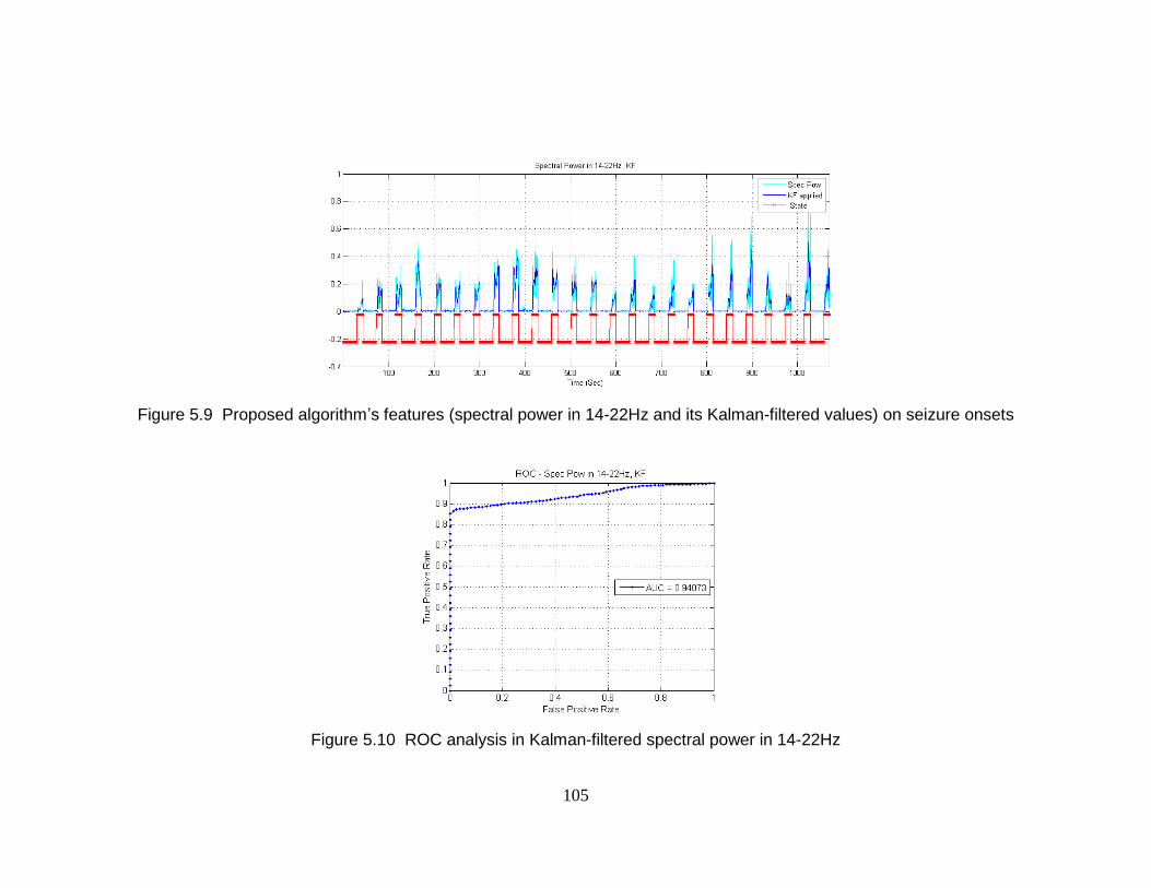
105

Figure 5.9 Proposed algorithm’s features (spectral power in 14-22Hz and its Kalman-filtered values) on seizure onsets

Figure 5.10 ROC analysis in Kalman-filtered spectral power in 14-22Hz

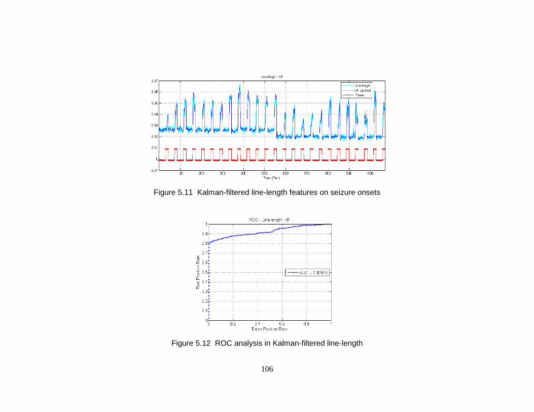
106

Figure 5.11 Kalman-filtered line-length features on seizure onsets

Figure 5.12 ROC analysis in Kalman-filtered line-length

107

In addition, sensitivity, the number of false positives, and the average latency time

between actual onsets and alarms generated by the algorithm have been estimated. Those

statistics are evaluated with two onset threshold values, which are out of the 100

threshold values used in the ROC analysis. One threshold values is the lowest threshold

value where the algorithm can produce sensitivity of 100% with no false positives: 0.55.

The estimated average latency is 3.23-sec. The other is the maximum threshold

algorithm without producing false positives. The threshold value is 0.14 and the

algorithm with that value achieves sensitivity of 100% and 4 false positives with the

average latency of 2.26-sec.

Proposed Approach for Onset Detection Using Spectral 5. 3. 2

Power in 14-22Hz and the Kalman Filter

The proposed feature used in our enhanced algorithm is the 2-tap Kalman-filtered

spectral power in 14-22Hz. We have selected the noise ratio between process noise and

measurement noise in the Kalman filter as 2-10

. Figure 5.9 illustrates the features of

spectral power in 14-22Hz in cyan and their 2-tap Kalman-filtered outputs in blue. Also,

the red line represents their true states: high for ictal and low for preictal.

The ROC analysis has been performed as well. The result of this analysis is

illustrated in Figure 5.10 and the AUC is estimated as 0.94083. It is noted that even

though the proposed algorithm presents the best performance in this chapter, its AUC is

smaller than that of the others. The AUC does not represent the detection rate well,

because while the actual detection rate should be based on the number of seizure events,

the AUC is calculated based on the number of windows.

108

Out of the 100 threshold values used in the ROC analysis, the lowest value of the

threshold with 100% sensitivity and no FPs is 0.0278, and its average latency is 2.10-sec.

With the threshold of 0.0147, the algorithm has generated 2 FPs as well as 100%

sensitivity with the average latency of 1.72-sec.

Approach for Onset Detection Using Line-Length 5. 3. 3

Additionally, we have tested the line-length as another feature. The line length was

proposed by Esteller et al. [57, 95], who is a scientist at NeuroPace, and it has been used

for seizure detection feature sets:

( )

∑ [ ( ) ( )]

where LL(n) is the line length, x(k) the kth

signal in a window of N samples, and K the

normalization constant.

In the same approach as the proposed enhanced approach but using the line length

as a feature, this approach shows the AUC of 0.92514 (See Figure 5.12). The lowest

threshold that reaches 100% sensitivity with no FPs is 0.033 and it shows the average

latency of 2.62-sec. With the threshold of 0.031, it produces 2FPs with the average

latency of 2.48-sec.

Result Comparison for Onset Detection 5. 3. 4

The results that come from the above three different methods for onset detection in rats’

ECoG recordings are summarized and compared in Table 5.1. Among these three, the

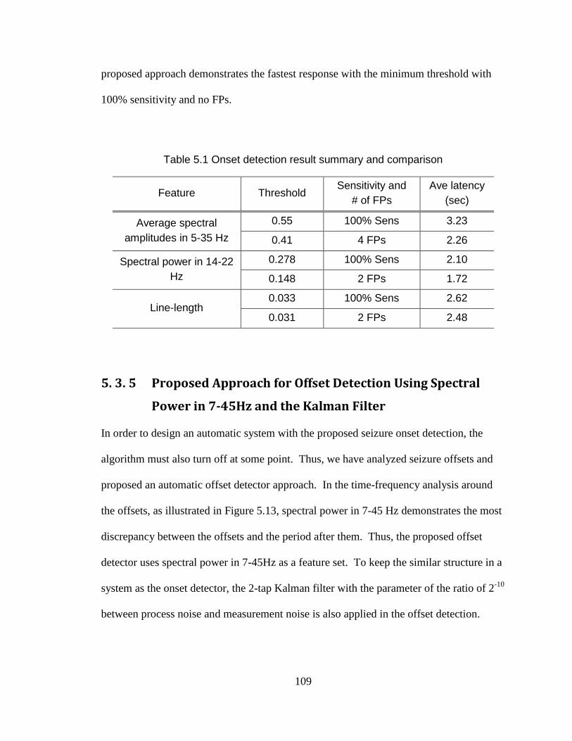
109

proposed approach demonstrates the fastest response with the minimum threshold with

100% sensitivity and no FPs.

Table 5.1 Onset detection result summary and comparison

Feature Threshold Sensitivity and

# of FPs

Ave latency

(sec)

Average spectral

amplitudes in 5-35 Hz

0.55 100% Sens 3.23

0.41 4 FPs 2.26

Spectral power in 14-22

Hz

0.278 100% Sens 2.10

0.148 2 FPs 1.72

Line-length 0.033 100% Sens 2.62

0.031 2 FPs 2.48

Proposed Approach for Offset Detection Using Spectral 5. 3. 5

Power in 7-45Hz and the Kalman Filter

In order to design an automatic system with the proposed seizure onset detection, the

algorithm must also turn off at some point. Thus, we have analyzed seizure offsets and

proposed an automatic offset detector approach. In the time-frequency analysis around

the offsets, as illustrated in Figure 5.13, spectral power in 7-45 Hz demonstrates the most

discrepancy between the offsets and the period after them. Thus, the proposed offset

detector uses spectral power in 7-45Hz as a feature set. To keep the similar structure in a

system as the onset detector, the 2-tap Kalman filter with the parameter of the ratio of 2-10

between process noise and measurement noise is also applied in the offset detection.

110

Testing Proposed Algorithm in Continuous Recording 5. 3. 6

The proposed algorithm extracts features of spectral power in 14-22Hz for onset

detection and that in 7-45Hz for offset detection and employs the 2-tap Kalman filter for

postprocessing. We have tested the proposed onset and offset detection algorithm in

continuous recordings (See Figure 5.14).

In Figure 5.14, there are four seizure onsets approximately at 85, 270, 580, and

660 seconds and offsets approximately at 180, 540, 630, and 770 seconds (See the top

panel in Figure 5.14). The middle panel illustrates the onset features of spectral power in

14-22Hz and the offset ones in 7-45Hz. The bottom panel demonstrates the algorithm’s

final outputs, and all of them match the corresponding onsets and offsets perfectly. The

parameters used in the algorithm are as follows: onset threshold of 0.0278 with the

Kalman filter’s ratio parameter of 2-10

and offset threshold of 0.001 with the parameter of

2-20

. It is noted that a seizure offset has been defined when the algorithm’s output keeps

lower than the offset threshold for five consecutive windows.

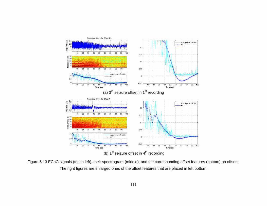
111

(a) 3

rd seizure offset in 1

st recording

(b) 1

st seizure offset in 4

th recording

Figure 5.13 ECoG signals (top in left), their spectrogram (middle), and the corresponding offset features (bottom) on offsets.

The right figures are enlarged ones of the offset features that are placed in left bottom.

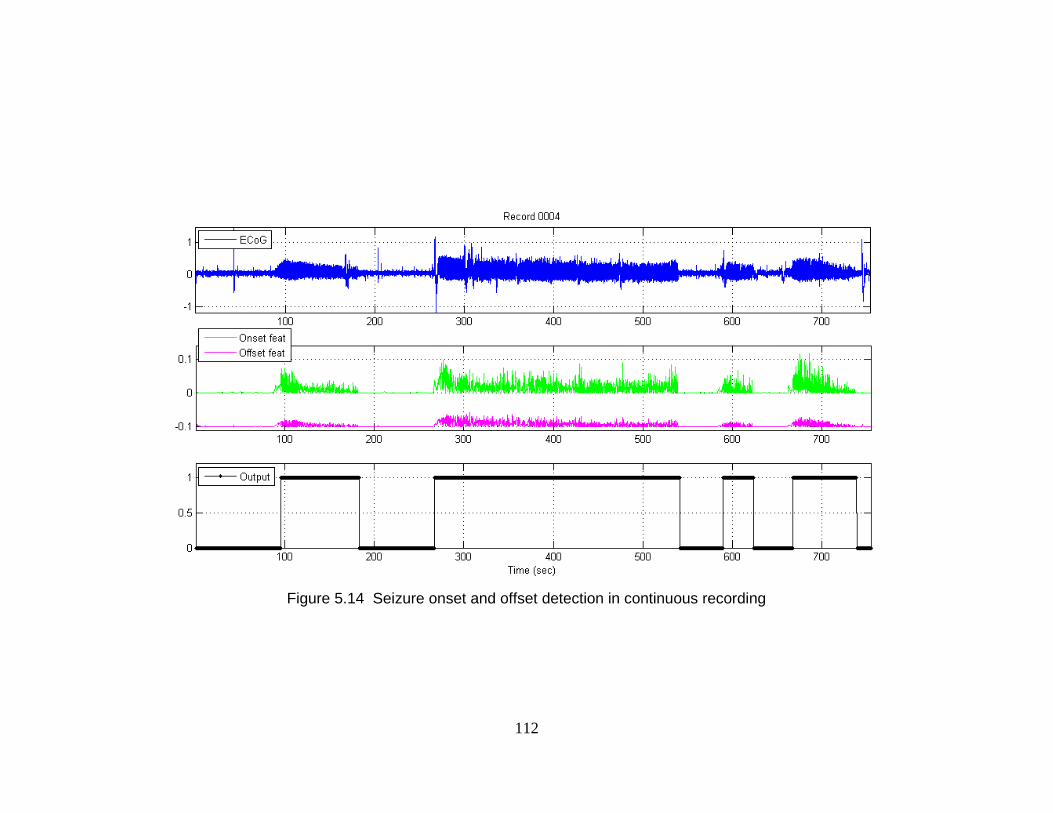
112

Figure 5.14 Seizure onset and offset detection in continuous recording

113

Discussions 5. 4

We have proposed an enhanced algorithm for seizure onset and offset detection in rats’

ECoG recordings. It has been improved by the following methods. First, the proposed

algorithm employs spectral power in 14-22 Hz as a feature. We have observed that the

spectral power feature is more effective for onset detection than the prior feature set of

spectral amplitudes in 5-35 Hz and the line-length feature. For example, as shown in

Table 5.1, the first two false positives begin to appear when the threshold value for the

proposed feature of spectral power decreases approximately 47% of the lowest threshold

value that produces no false positives and sensitivity of 100%. Similarly, the first two or

more false positives begin to appear when the threshold values of the prior feature and

line-length decrease approximately 25% and 6 of the lowest threshold values with no

false positives and perfect sensitivity, respectively.

Furthermore, postprocessing spectral power features in 14-22Hz by the 2-tap

Kalman filter improves onset detection. The Kalman-filtered features in the proposed

algorithm have been observed to be very effective to significantly reduce the number of

potential false positives. For example, the following three postprocessed features at a

certain onset are compared in Figure 5.15: 2-point moving-averaged spectral amplitudes

in 5-35Hz (left, the prior approach), 2-tap Kalman-filtered spectral power in 14-22Hz

(middle, the proposed approach), and 2-tap Kalman-filtered line-length (right, additional

approach). While 2-point moving-averaged spectral amplitudes and the Kalman-filtered

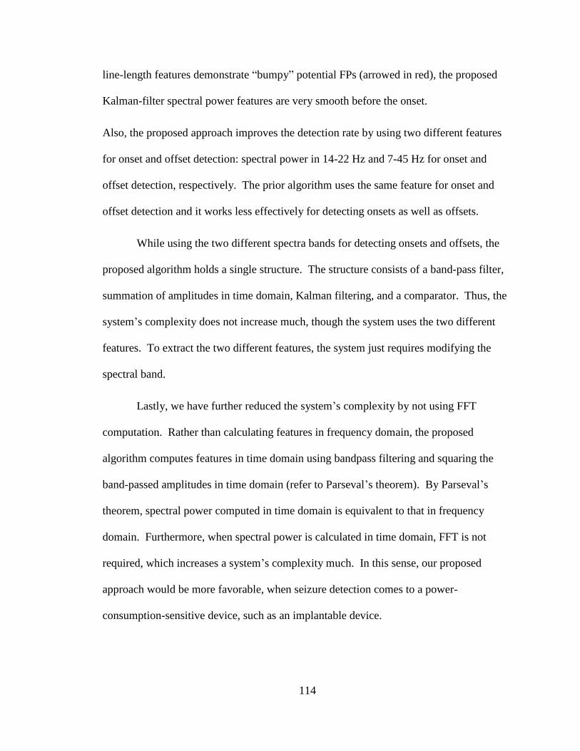
114

line-length features demonstrate “bumpy” potential FPs (arrowed in red), the proposed

Kalman-filter spectral power features are very smooth before the onset.

Also, the proposed approach improves the detection rate by using two different features

for onset and offset detection: spectral power in 14-22 Hz and 7-45 Hz for onset and

offset detection, respectively. The prior algorithm uses the same feature for onset and

offset detection and it works less effectively for detecting onsets as well as offsets.

While using the two different spectra bands for detecting onsets and offsets, the

proposed algorithm holds a single structure. The structure consists of a band-pass filter,

summation of amplitudes in time domain, Kalman filtering, and a comparator. Thus, the

system’s complexity does not increase much, though the system uses the two different

features. To extract the two different features, the system just requires modifying the

spectral band.

Lastly, we have further reduced the system’s complexity by not using FFT

computation. Rather than calculating features in frequency domain, the proposed

algorithm computes features in time domain using bandpass filtering and squaring the

band-passed amplitudes in time domain (refer to Parseval’s theorem). By Parseval’s

theorem, spectral power computed in time domain is equivalent to that in frequency

domain. Furthermore, when spectral power is calculated in time domain, FFT is not

required, which increases a system’s complexity much. In this sense, our proposed

approach would be more favorable, when seizure detection comes to a power-

consumption-sensitive device, such as an implantable device.

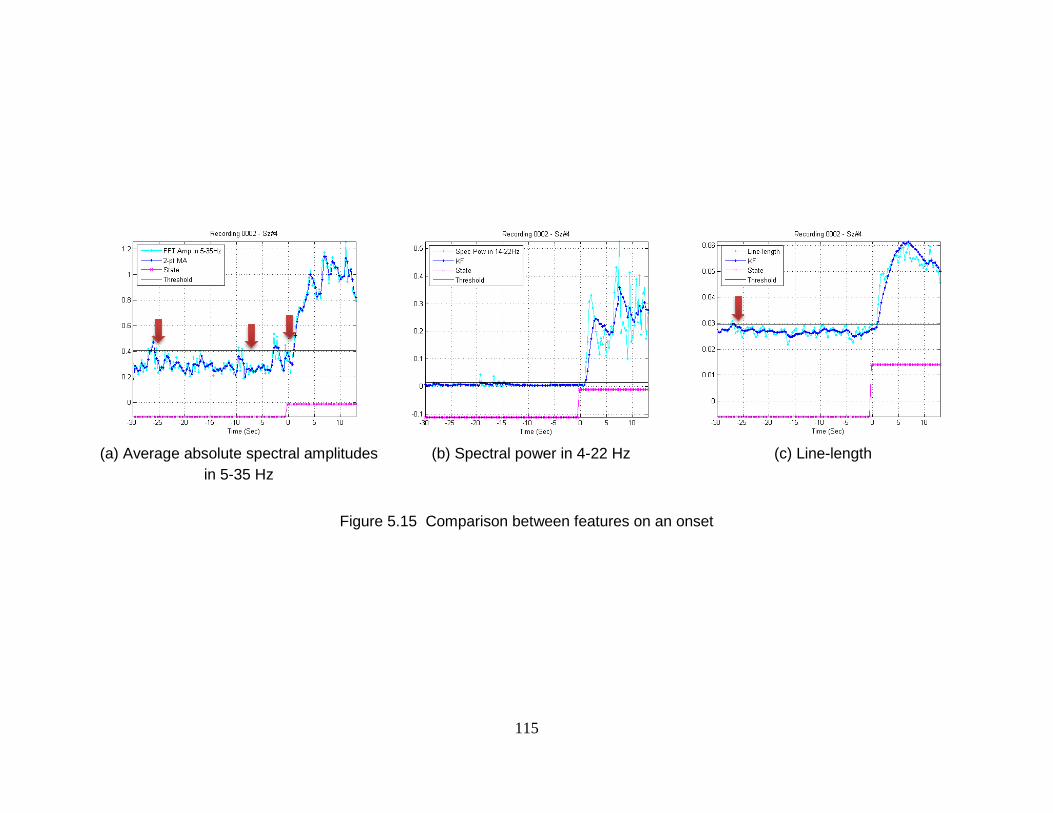
115

(a) Average absolute spectral amplitudes

in 5-35 Hz

(b) Spectral power in 4-22 Hz

(c) Line-length

Figure 5.15 Comparison between features on an onset

116

Conclusion 5. 5

We have proposed an enhanced automatic seizure onset and offset detection algorithm.

As a feature set, it uses spectral power in 14-22 Hz for onset detection and that in 7-45Hz

for offset detection. In addition, it employs a Kalman filter for postprocessing.

Compared to a prior approach, which uses spectral amplitudes and 2-point moving

average, the proposed algorithm is more accurate, detects onsets and offsets faster, and

has less complexity.

117

Chapter 6

Conclusions and Future Research

Directions

Conclusions 6. 1

This thesis focuses on developing approaches that can classify electrocorticogram (ECoG)

and/or intracranial electroencephalogram (iEEG) for human epileptic seizure prediction

using linear features and machine-learning-based classification approaches. The thesis

further investigates methods to reduce complexity of the seizure prediction approach and

proposes a reduced-complexity seizure prediction algorithm that uses less number of

features and a linear SVM classifier.

The long-term goal of the research is to prototype an implantable device that can

reliably provide alarms prior to a seizure in real-time, and the specific objective is to

develop a reduced-complexity patient-specific algorithm that can predict seizures with

ECoG/iEEG with high sensitivity and low false positive rate. Seizure prediction is such a

118

challenging problem that many researchers have achieved only partial successes, for

example, in their own recordings or in short recordings [1, 89]. It is mainly because

signal patterns across subjects vary significantly and no single measures have been found

as a successful solution to prediction.

This dissertation has demonstrated that human epileptic seizures can be predicted

with linear features of ECoG/iEEG by machine learning and the Kalman filter.

Furthermore, we have reduced the algorithm’s complexity to be feasible for an

implantable device. Besides the seizure prediction work, additionally, we have proposed

an enhanced a seizure detection approach for in-vivo rats with ECoG.

Seizure Prediction with Spectral Power of ECoG/iEEG 6. 1. 1

using SVMs

We have investigated the human epileptic seizure prediction problem and have tested the

hypothesis that seizures could be predicted using linear features of spectral power from

ECoG/iEEG. It is noted that extracting linear features do not require power as much as

extracting nonlinear features and thus using linear features is advantageous for an

implantable device. With 27 to 54 linear features of spectral power extracted from

ECoG/iEEG, we have developed a human seizure prediction algorithm by using machine

learning techniques based on SVMs [10, 89]. The method of double cross-validation in

the algorithm ensures in-sample optimization and out-of-sample testing for the SVM to

determine estimated models are neither over-fitted nor under-fitted [14]. Preprocessing

with the bipolar and/or time-differential method and postprocessing with the Kalman

filter lowered the false positive rate significantly while maintaining high sensitivity.

119

Reduced Complexity Seizure Prediction with Linear SVMs 6. 1. 2

For our seizure prediction algorithm to be practically used on an implantable device, it is

necessary to reduce its complexity. It is mainly because the above proposed algorithm

requires high power consumption in extracting the 27-54 features and using nonlinear

SVMs. This would be a prohibitive factor for the algorithm to be installed on a real-time

implantable device [56].

We have proposed a reduced-complexity seizure prediction algorithm. The

methods in lowering the complexity are as follows. We reduce the number of features by

investigating the subset of key features using the RFE SVM [85]. Also, the SVMs with

the radial basis function (RBF) kernel are replaced by linear SVMs. Furthermore, the

Kalman filter is substituted with the 20-tap moving-average filter. Using these three

methods, a reduced-complexity seizure prediction algorithm has been proposed, which

significantly lowers the system’s complexity and thus the power consumption, while

producing high sensitivity as well as reasonable false positive rate.

Enhanced Seizure Detection with Rat’s ECoG 6. 1. 3

Prof. Yang, one of our colleagues, developed an automated seizure detection and

termination system for experiments in in-vivo rats [15]. We have developed an improved

detection approach to reduce false positive rate and the latency between the detector’s

alarm and the actual onset, while maintaining high sensitivity. We have investigated

time-frequency patterns of rats’ ECoG around the onsets by spectrogram. We have

observed that the performance of the seizure detector can be significantly enhanced by

using the narrowed frequency range of 14-22Hz rather than 5 -35Hz, with spectral power

120

instead of spectral amplitudes as a feature set, and replacing the 2-point moving average

filter by a Kalman filter.

Future Research Directions 6. 2

We would like to extend our research as follows: (1) extending our seizure prediction

analysis onto the Mayo database; (2) testing wavelets and other pre-defined values; (3)

using other approaches for the binary classification and investigation of key features; (4)

implementing the proposed seizure detection method in rats’ ECoG in LabVIEW; (5)

investigating hardware architectures for real-time implantable seizure predictors; and (6)

extending our combined approach of signal processing and machine learning to other

neural problems.

Extending and validating our prediction approach onto the 6. 2. 1

larger database of Mayo

Future work will address applications of our analysis to the Mayo dataset for larger scale

testing of the algorithm. This dataset has been collected at the Mayo Clinic by Dr.

Gregory Worrell, M.D., Ph.D., and is available for analysis. We have concentrated on

developing and testing our algorithm for seizure prediction based on a relatively small

dataset. By expanding our analysis to a much larger dataset, we may test the robustness

of the algorithm under more realistic conditions. The Mayo dataset contains iEEG

recordings of approximately 30 patients undergoing diagnosis for epilepsy. Each patient

has between 20 and 128 electrodes, and the recordings are at least 72 hours long and

121

include on average 3 to 5 seizures. The entire database is approximately 15 Terabytes in

size and growing. All the patients have signed release forms in accordance with Mayo

Clinic Institutional Review Board rules and we have also obtained an IRB‐approved

protocol for this study at the University of Minnesota (IRB‐0906M67881).

The Mayo dataset has several advantages over the Freiburg datasets. The Mayo

dataset has been recorded using a complete set of electrodes, rather than a couple of

electrodes located at seizure focus. In addition, they are much more comprehensive,

covering the activity of the patient for much longer periods of time. Analysis with the

Mayo dataset will be one of the largest seizure prediction projects undertaken. Thus, we

will be able to provide the results with more credibility and more reliability than those

developed based on a small sampling of patients.

Improving the predictor by testing wavelet features and 6. 2. 2

finding optimized parameters in the algorithm

In the thesis, we have developed a reliable seizure prediction approach using spectral

power features from ECoG/iEEG, and the approach’s complexity has been reduced by

investigating key features and using the linear classifier and filter for postprocessing.

The reduced-complexity seizure prediction approach may be further improved by

replacing the spectral power features with wavelet features. In this thesis, the spectral

power features were extracted in standard EEG frequency bands, and the higher

frequency bands have the larger bandwidths. This represents that the spectral power

features may be seamlessly substituted by wavelet features. The wavelet features are

122

expected not only to produce prediction rate as high as the spectral power features but

also to further reduce the complexity.

Some parameters in the proposed algorithm were operationally defined: for

example, 20-sec moving-windows with half-overlap, 30-min preictal in length, and

several frequency bands in feature extraction. By investigating more optimized lengths

for the moving-window and preictal prediction horizon and more effective frequency

bands for spectral power features, we may be able to propose a better prediction approach.

Furthermore, we can seek those optimized values in patient-specific manner. For

example, patient-specific preictal prediction horizons would provide better prediction rate,

because some patients may have shorter or longer preictal phases.

Testing other classification methods and investigating key 6. 2. 3

features using other approaches

Using linear and nonlinear SVMs, we have achieved the excellent result for seizure

prediction; however, there may be better classification approaches than the SVMs, which

may produce better prediction rate with less complexity. They include AdaBoost, Neural

Networks, and Bayses classifiers as a single classification method. Also, decision fusion,

which is a combined classification approach of making a global decision based on

multiple local decisions [96], can be employed for seizure prediction.

In Chapter 4, we have investigated a subset of key features using the RFE SVM.

There are a variety of methods for feature selection [85, 86], including Fast Correlation-

Based Feature Selection [97] and Weighted Naïve Bayes [98]. By using the other key

123

feature techqniues, we may be able to compare subsets of key features and investigate

critical features.

Implementing the proposed algorithm for enhanced 6. 2. 4

seizure detection with in-vivo rats’ ECoG in LabVIEW

In the thesis, we have proposed an enhanced algorithm for seizure detection with in-vivo

rats’ ECoG. Compared to Yang et al.’s work proposed in [15-17], our algorithm is

expected to reduce the number of false positives, respond onsets promptly, and lower the

system’s complexity, while providing high sensitivity and specificity. It would be

interesting if our enhanced algorithm is implemented in hardware in LabVIEW and tested

with in-vivo rats’ ECoG. Then, we could directly compare the prior approach and ours

on the actual hardware device in real-time.

Investigating hardware architectures for a real-time 6. 2. 5

seizure predictor and developing it in hardware

We have proposed an algorithm for seizure prediction with linear features of ECoG/iEEG

using SVM classification and Kalman filtering [89], and we have further proposed a

reduced-complexity prediction algorithm to be feasible for an implantable device.

Considering our ultimate goal of implementing an implantable device for real-time

seizure prediction, beyond the algorithm design, it is necessary to investigate hardware

architectures. We believe that there is great room for improvement on hardware

architectures for a real-time seizure predictor, because they require low complexity for

low power consumption.

124

Furthermore, we consider to develop an automatic real-time implantable device

on a neural system, such as Neural Interface System [99]. Ultimately, we will extend it

into an automatic closed-loop system that provides an alarm ahead of a seizure attack and

triggers rescue therapy, such as deep brain stimulation [7].

Extending the machine-learning-based classification to 6. 2. 6

other neuronal applications

In our seizure prediction work, we have incorporated techniques of machine learning and

statistical model estimation to the neural signal processing. From the seizure applications,

we can extend this approach to other neuronal applications. Specifically, our approach

can be beneficial to brain signal processing, because brain signal mechanisms are too

complex to be understood and the machine learning approach can provide statistical

methodologies for estimating and understanding the “X” box of the brain. For example,

our approach can be applied to estimating real-time neural decoding algorithms for multi-

dimensional movement from persons with tetraplegia [100] and for reach-and-grasp

movement from a small population of M1 arm/hand area neurons [101].

125

Bibliography

[1] F. Mormann, R. Andrzejak, C. Elger, and K. Lehnertz, "Seizure prediction: the long and

winding road," Brain, vol. 130, p. 314, 2007.

[2] B. Schelter, J. Timmer, and A. Schulze-Bonhage, Seizure prediction in epilepsy: from

basic mechanisms to clinical applications: Vch Pub, 2008.

[3] J. F. Annegers, The epidemiology of epilepsy, 1996.

[4] C. E. Elger, "Future trends in epileptology," Current Opinion in Neurology, vol. 14, pp.

185-186, Apr 2001.

[5] Y. Park, L. Luo, K. K. Parhi, and T. Netoff, "Seizure prediction with spectral power of

EEG using cost-sensitive support vector machines," Epilepsia, vol. 52, pp. 1761-1770,

Oct 2011.

[6] K. N. Fountas and J. Smith, "A novel closed-loop stimulation system in the control of

focal, medically refractory epilepsy," Operative Neuromodulation, pp. 357-362, 2007.

[7] R. Fisher, V. Salanova, T. Witt, R. Worth, T. Henry, R. Gross, K. Oommen, I. Osorio, J.

Nazzaro, and D. Labar, "Electrical stimulation of the anterior nucleus of thalamus for

treatment of refractory epilepsy," Epilepsia, vol. 51, pp. 899-908, 2010.

[8] B. Litt and J. Echauz, "Prediction of epileptic seizures," Lancet Neurology, vol. 1, pp. 22-

30, 2002.

[9] T. Netoff, Y. Park, and K. Parhi, "Seizure prediction using cost-sensitive support vector

machine," in IEEE Engineering in Medicine and Biology Society, Minneapolis, MN,

USA, 2009, pp. 3322-3325.

[10] Y. Park, T. Neoff, and K. Parhi, "Seizure prediction with spectral power of time/space-

differential EEG signals using cost-sensitive support vector machine," in ICASSP, Dallas,

TX, USA, 2010, pp. 5450-5453.

[11] F. Mormann, T. Kreuz, C. Rieke, R. Andrzejak, A. Kraskov, P. David, C. Elger, and K.

Lehnertz, "On the predictability of epileptic seizures," Clinical Neurophysiology, vol. 116,

pp. 569-587, 2005.

[12] B. Litt, R. Esteller, J. Echauz, M. D'Alessandro, R. Shor, T. Henry, P. Pennell, C. Epstein,

R. Bakay, M. Dichter, and G. Vachtsevanos, "Epileptic seizures may begin hours in

advance of clinical onset: A report of five patients," Neuron, vol. 30, pp. 51-64, Apr 2001.

[13] J. H. Friedman, "An overview of predictive learning and function approximation," in

From statistics to neural networks: Theory and pattern recognition applications (NATO

ASI Series / Computer and Systems Sciences). vol. 136, V. Cherkassky, J. H. Friedman,

and H. Wechsler, Eds., 2 ed Berlin: Springer, 1994, pp. 1-61.

[14] V. Cherkassky and F. Mulier, Learning from data: Concepts, theory, and methods.

Hoboken: Wiley-Interscience, 2007.

[15] X. F. Yang, D. W. Duffy, R. E. Morley, and S. M. Rothman, "Neocortical seizure

termination by focal cooling: temperature dependence and automated seizure detection,"

Epilepsia, vol. 43, pp. 240-245, 2002.

126

[16] X. F. Yang and S. M. Rothman, "Focal cooling rapidly terminates experimental

neocortical seizures," Annals of Neurology, vol. 49, pp. 721-726, 2001.

[17] X. Yang, B. Schmidt, D. Rode, and S. Rothman, "Optical suppression of experimental

seizures in rat brain slices," Epilepsia, vol. 51, pp. 127-135, 2009.

[18] Available: http://www.epilepsyfoundation.org/about/statistics.cfm

[19] Available: http://www.efwp.org/programs/side_effects.shtml

[20] A. Handforth, "Vagus nerve stimulation therapy for partial-onset seizures," Epilepsia, vol.

29, pp. 721-730, 1988.

[21] L. Nashef and R. Selway, "Vagus nerve stimulation," Epilepsy, pp. 449-453, 2009.

[22] A. Shahwan, C. Bailey, W. Maxiner, and A. S. Harvey, "Vagus nerve stimulation for

refractory epilepsy in children: more to VNS than seizure frequency reduction," Epilepsia,

vol. 50, pp. 1220-1228, 2009.

[23] S. Rothman, M. Smyth, X. Yang, and G. Peterson, "Focal cooling for epilepsy: an

alternative therapy that might actually work," Epilepsy & Behavior, vol. 7, pp. 214-221,

2005.

[24] NeuroPace. NeuroPace RNS System. Available:

http://www.neuropace.com/product/overview.html

[25] E. Wyllie, A. Gupta, and K. Lachhwani, The treatment of epilepsy: principles & practice,

4th ed.: Lippincott Williams & Wilkins, 2005.

[26] V. Strong, S. Brown, and R. Walker, "Seizure-alert dogs--fact or fiction?," Seizure, vol. 8,

pp. 62-65, 1999.

[27] S. W. Brown and V. Strong, "The use of seizure-alert dogs," Seizure, vol. 10, pp. 39-41,

2001.

[28] D. J. Dalziel, B. M. UTHMAN, S. P. MCGORRAY, and R. L. REEP, "Seizure-alert dogs:

a review and preliminary study," Seizure, vol. 12, pp. 115-120, 2003.

[29] V. StrongStephen, "Effect of trained Seizure Alert Dogs® on frequency of tonic-clonic

seizures," Seizure, vol. 11, pp. 402-405, 2002.

[30] H. Jasper, "Some physiological mechanisms involved in epileptic automatisms,"

Epilepsia, vol. 5, pp. 1-20, 1964.

[31] C. Baumgartner, W. Serles, F. Leutmezer, E. Pataraia, S. Aull, T. Czech, U. Pietrzyk, A.

Relic, and I. Podreka, "Preictal SPECT in temporal lobe epilepsy: regional cerebral blood

flow is increased prior to electroencephalography-seizure onset," Journal of Nuclear

Medicine, vol. 39, p. 978, 1998.

[32] V. Novak, A. L. Reeves, P. Novak, P. A. Low, and F. W. Sharbrough, "Time-frequency

mapping of RR interval during complex partial seizures of temporal lobe origin," Journal

of the Autonomic Nervous System, vol. 77, pp. 195-202, 1999.

[33] R. S. Delamont, P. O. O. Julu, and G. A. Jamal, "Changes in a measure of cardiac vagal

activity before and after epileptic seizures," Epilepsy Research, vol. 35, pp. 87-94, 1999.

[34] C. Schernthaner, G. Lindinger, K. Pötzelberger, K. Zeiler, and C. Baumgartner,

"Autonomic epilepsy--the influence of epileptic discharges on heart rate and rhythm,"

Wiener Klinische Wochenschrift, vol. 111, p. 392, 1999.

127

[35] S. Viglione and G. Walsh, "Proceedings: Epileptic seizure prediction,"

Electroencephalography and Clinical Neurophysiology, vol. 39, p. 435, 1975.

[36] Z. Rogowski, I. Gath, and E. Bental, "On the prediction of epileptic seizures," Biological

Cybernetics, vol. 42, pp. 9-15, 1981.

[37] Y. Salant, I. Gath, and O. Henriksen, "Prediction of epileptic seizures from two-channel

EEG," Medical and Biological Engineering and Computing, vol. 36, pp. 549-556, 1998.

[38] H. H. Lange, J. P. Lieb, J. Engel Jr, and P. H. Crandall, "Temporo-spatial patterns of pre-

ictal spike activity in human temporal lobe epilepsy," Electroencephalography and

Clinical Neurophysiology, vol. 56, pp. 543-555, 1983.

[39] A. Katz, D. A. Marks, G. Mccarthy, and S. S. Spencer, "Does Interictal Spiking Change

Prior to Seizures," Electroencephalography and Clinical Neurophysiology, vol. 79, pp.

153-156, Aug 1991.

[40] L. D. Iasemidis, J. Chris Sackellares, H. P. Zaveri, and W. J. Williams, "Phase space

topography and the Lyapunov exponent of electrocorticograms in partial seizures," Brain

Topography, vol. 2, pp. 187-201, 1990.

[41] H. Moser, B. Weber, H. Wieser, and P. Meier, "Electroencephalograms in epilepsy:

analysis and seizure prediction within the framework of Lyapunov theory," Physica D:

Nonlinear Phenomena, vol. 130, pp. 291-305, 1999.

[42] D. Lerner, "Monitoring changing dynamics with correlation integrals: case study of an

epileptic seizure," Physica D: Nonlinear Phenomena, vol. 97, pp. 563-576, 1996.

[43] J. Martinerie, C. Adam, M. Le Van Quyen, M. Baulac, S. Clemenceau, B. Renault, and F.

Varela, "Epileptic seizures can be anticipated by non-linear analysis," Nature Medicine,

vol. 4, pp. 1173-1176, 1998.

[44] K. Lehnertz and C. Elger, "Can epileptic seizures be predicted? Evidence from nonlinear

time series analysis of brain electrical activity," Physical Review Letters, vol. 80, pp.

5019-5022, 1998.

[45] M. L. Van Quyen, J. Martinerie, M. Baulac, and F. Varela, "Anticipating epileptic

seizures in real time by a non-linear analysis of similarity between EEG recordings,"

Neuroreport, vol. 10, p. 2149, 1999.

[46] M. Le Van Quyen, J. Martinerie, V. Navarro, P. Boon, M. D'Havé, C. Adam, B. Renault,

F. Varela, and M. Baulac, "Anticipation of epileptic seizures from standard EEG

recordings," The Lancet, vol. 357, pp. 183-188, 2001.

[47] J. Sackellares, D. Shiau, J. Principe, M. Yang, L. Dance, W. Suharitdamrong, W.

Chaovalitwongse, P. Pardalos, and L. Iasemidis, "Predictability analysis for an automated

seizure prediction algorithm," Journal of Clinical Neurophysiology, vol. 23, p. 509, 2006.

[48] M. Harrison, I. Osorio, M. Frei, S. Asuri, and Y. Lai, "Correlation dimension and integral

do not predict epileptic seizures," Chaos, vol. 15, p. 033106, 2005.

[49] R. Aschenbrenner-Scheibe, T. Maiwald, M. Winterhalder, H. Voss, J. Timmer, and A.

Schulze-Bonhage, "How well can epileptic seizures be predicted? An evaluation of a

nonlinear method," Brain, vol. 126, p. 2616, 2003.

[50] W. De Clercq, P. Lemmerling, S. Van Huffel, and W. Van Paesschen, "Anticipation of

epileptic seizures from standard EEG recordings," The Lancet, vol. 361, p. 971, 2003.

128

[51] Y. C. Lai, M. A. F. Harrison, M. G. Frei, and I. Osorio, "Inability of Lyapunov exponents

to predict epileptic seizures," Physical Review Letters, vol. 91, p. 68102, 2003.

[52] Y. C. Lai, M. A. F. Harrison, M. G. Frei, and I. Osorio, "Controlled test for predictive

power of Lyapunov exponents: their inability to predict epileptic seizures," Chaos: An

Interdisciplinary Journal of Nonlinear Science, vol. 14, p. 630, 2004.

[53] K. Jerger, T. Netoff, J. Francis, T. Sauer, L. Pecora, S. Weinstein, and S. Schiff, "Early

seizure detection," Journal of Clinical Neurophysiology, vol. 18, p. 259, 2001.

[54] J. Milton and P. Jung, Epilepsy as a dynamic disease: Springer Verlag, 2003.

[55] I. Osorio, M. Frei, and S. Wilkinson, "Real-time automated detection and quantitative

analysis of seizures and short-term prediction of clinical onset," Epilepsia, vol. 39, pp.

615-627, 1998.

[56] A. Shoeb, D. Carlson, E. Panken, and T. Denison, "A micro support vector machine

based seizure detection architecture for embedded medical devices," in IEEE Engineering

in Medicine and Biology Society, Minneapolis, MN, USA, 2009, pp. 4202-4205.

[57] A. B. Gardner, A. M. Krieger, G. Vachtsevanos, and B. Litt, "One-class novelty detection

for seizure analysis from intracranial EEG," The Journal of Machine Learning Research,

vol. 7, pp. 1025-1044, 2006.

[58] A. Shoeb, S. Schachter, D. Schomer, B. Bourgeois, S. Treves, and J. Guttag, "Detecting

seizure onset in the ambulatory setting: demonstrating feasibility," presented at the IEEE

Engineering in Medicine and Biology Society, Shanghai, China, 2005.

[59] M. Nandan, S. Talathi, S. Myers, W. Ditto, P. Khargonekar, and P. Carney, "Support

vector machines for seizure detection in an animal model of chronic epilepsy," Journal of

Neural Engineering, vol. 7, p. 036001, 2010.

[60] L. Chisci, A. Mavino, G. Perferi, M. Sciandrone, C. Anile, G. Colicchio, and F. Fuggetta,

"Real-Time Epileptic Seizure Prediction Using AR Models and Support Vector

Machines," IEEE transactions on bio-medical engineering, vol. 57, pp. 1124-1132, 2010.

[61] E. Alpaydin, Introduction to machine learning. Cambridge: The MIT Press, 2004.

[62] S. Stanslaski, P. Cong, D. Carlson, W. Santa, R. Jensen, G. Molnar, W. J. Marks, A.

Shafquat, and T. Denison, "An implantable bi-directional brain-machine interface system

for chronic neuroprosthesis research," 2009, pp. 5494-5497.

[63] V. Vapnik, The nature of statistical learning theory. New York: Springer, 2000.

[64] D. Moore and G. McCabe, Introduction to the Practice of Statistics. New York: W.H.

Freeman, 2005.

[65] D. Simon, Optimal state estimation: Kalman, H [infinity] and nonlinear approaches.

Hoboken: John Wiley and Sons, 2006.

[66] G. Welch and G. Bishop, "An introduction to the Kalman filter," University of North

Carolina at Chapel Hill, Chapel Hill, NC, vol. 7, 1995.

[67] S. M. Beitzel, "On understanding and classifying web queries," Citeseer, 2006.

[68] K. Lehnertz, F. Mormann, H. Osterhage, A. Muller, J. Prusseit, A. Chernihovskyi, M.

Staniek, D. Krug, S. Bialonski, and C. Elger, "State-of-the-art of seizure prediction,"

Journal of Clinical Neurophysiology, vol. 24, pp. 147-153, 2007.

129

[69] D. Snyder, J. Echauz, D. Grimes, and B. Litt, "The statistics of a practical seizure

warning system," Journal of Neural Engineering, vol. 5, p. 392, 2008.

[70] R. G. Andrzejak, F. Mormann, T. Kreuz, C. Rieke, A. Kraskov, C. E. Elger, and K.

Lehnertz, "Testing the null hypothesis of the nonexistence of a preseizure state," Physical

Review E, vol. 67, p. 010901, 2003.

[71] R. Andrzejak, D. Chicharro, C. Elger, and F. Mormann, "Seizure prediction: Any better

than chance?," Clinical Neurophysiology, vol. 120, pp. 1465-1478, 2009.

[72] J. Huang and C. X. Ling, "Using AUC and accuracy in evaluating learning algorithms,"

Ieee Transactions on Knowledge and Data Engineering, vol. 17, pp. 299-310, Mar 2005.

[73] T. Fawcett, "An introduction to ROC analysis," Pattern Recognition Letters, vol. 27, pp.

861-874, Jun 2006.

[74] Freiburg EEG database. Available: https://epilepsy.uni-freiburg.de/freiburg-seizure-

prediction-project/eeg-database

[75] P. Nunez and R. Srinivasan, Electric fields of the brain: the neurophysics of EEG. New

York: Oxford University Press, 2006.

[76] B. Hjorth, "EEG analysis based on time domain properties," Electroencephalography and

clinical neurophysiology, vol. 29, p. 306, 1970.

[77] B. Schölkopf, C. Burges, and A. Smola, Advances in kernel methods: support vector

learning. Cambridge: The MIT press, 1999.

[78] S. Mika, G. Ratsch, J. Weston, B. Scholkopf, and K. Muller, "Fisher discriminant

analysis with kernels," in Neural Networks for Signal Processing IX, Madison, WI, USA,

1999, pp. 41–48.

[79] R. Andrzejak, F. Mormann, T. Kreuz, C. Rieke, A. Kraskov, C. Elger, and K. Lehnertz,

"Testing the null hypothesis of the nonexistence of a preseizure state," Physical review. E,

Statistical, nonlinear, and soft matter physics, vol. 67, p. 10901, 2003.

[80] T. Maiwald, M. Winterhalder, R. Aschenbrenner-Scheibe, H. Voss, A. Schulze-Bonhage,

and J. Timmer, "Comparison of three nonlinear seizure prediction methods by means of

the seizure prediction characteristic," Physica D. Nonlinear Phenomena, vol. 194, pp.

357-368, 2004.

[81] M. Winterhalder, T. Maiwald, H. Voss, R. Aschenbrenner-Scheibe, J. Timmer, and A.

Schulze-Bonhage, "The seizure prediction characteristic: a general framework to assess

and compare seizure prediction methods," Epilepsy and Behavior, vol. 4, pp. 318-325,

2003.

[82] P. Mirowski, D. Madhavan, Y. LeCun, and R. Kuzniecky, "Classification of patterns of

EEG synchronization for seizure prediction," Clinical Neurophysiology, vol. 120, pp.

1927-1940 2009.

[83] D. Tax and R. Duin, "Support vector data description," Machine Learning, vol. 54, pp.

45-66, 2004.

[84] A. Shoeb, D. Carlson, E. Panken, and T. Denison, "A micropower support vector

machine based seizure detection architecture for embedded medical devices," in

Engineering in Medicine and Biology Society, 2009. EMBC 2009. Annual International

Conference of the IEEE, 2009, pp. 4202-4205.

130

[85] I. Guyon and A. Elisseeff, "An introduction to variable and feature selection," Journal of

Machine Learning Research, vol. 3, pp. 1157-1182, 2003.

[86] Y. Saeys, I. Inza, and P. Larrañaga, "A review of feature selection techniques in

bioinformatics," Bioinformatics, vol. 23, pp. 2507-2517, 2007.

[87] I. Guyon, J. Weston, S. Barnhill, and V. Vapnik, "Gene selection for cancer classification

using support vector machines," Machine learning, vol. 46, pp. 389-422, 2002.

[88] T. Joachims, "SVM light, http://svmlight.joachims.org," 2002.

[89] Y. Park, L. Luo, K. K. Parhi, and T. Netoff, "Seizure prediction with spectral power of

EEG using cost sensitive support vector machines," Epilepsia, 2011.

[90] P. Baldi, S. Brunak, Y. Chauvin, C. A. Andersen, and H. Nielsen, "Assessing the

accuracy of prediction algorithms for classification: an overview," Bioinformatics, vol. 16,

pp. 412-24, May 2000.

[91] A. Rotenberg, P. Muller, D. Birnbaum, M. Harrington, J. J. Riviello, A. Pascual-Leone,

and F. E. Jensen, "Seizure suppression by EEG-guided repetitive transcranial magnetic

stimulation in the rat," Clinical Neurophysiology, vol. 119, pp. 2697-2702, 2008.

[92] F. Noè, A. H. Pool, J. Nissinen, M. Gobbi, R. Bland, M. Rizzi, C. Balducci, F. Ferraguti,

G. Sperk, and M. J. During, "Neuropeptide Y gene therapy decreases chronic

spontaneous seizures in a rat model of temporal lobe epilepsy," Brain, vol. 131, pp. 1506-

1515, 2008.

[93] A. Vezzani, M. Conti, A. De Luigi, T. Ravizza, D. Moneta, F. Marchesi, and M. G. De

Simoni, "Interleukin-1β immunoreactivity and microglia are enhanced in the rat

hippocampus by focal kainate application: functional evidence for enhancement of

electrographic seizures," The Journal of neuroscience, vol. 19, pp. 5054-5065, 1999.

[94] G. W. Mathern, F. Cifuentes, J. P. Leite, J. K. Pretorius, and T. L. Babb, "Hippocampal

EEG excitability and chronic spontaneous seizures are associated with aberrant synaptic

reorganization in the rat intrahippocampal kainate model," Electroencephalography and

Clinical Neurophysiology, vol. 87, pp. 326-339, 1993.

[95] R. Esteller, J. Echauz, T. Tcheng, B. Litt, and B. Pless, "Line length: an efficient feature

for seizure onset detection," 2001, pp. 1707-1710 vol. 2.

[96] M. Duarte and Y. Hu, "Distance-based decision fusion in a distributed wireless sensor

network," Telecommunication Systems, vol. 26, pp. 339-350, 2004.

[97] L. Yu and H. Liu, "Efficient feature selection via analysis of relevance and redundancy,"

Journal of Machine Learning Research, vol. 5, pp. 1205-1224, Oct 2004.

[98] R. O. Duda, P. E. Hart, and D. G. Stork, "Pattern classification," John Willey & Sons,

2001.

[99] J. P. Donoghue, A. Nurmikko, M. Black, and L. R. Hochberg, "Assistive technology and

robotic control using motor cortex ensemble based neural interface systems in humans

with tetraplegia," The Journal of Physiology, vol. 579, pp. 603-611, 2007.

[100] S. P. Kim, J. D. Simeral, L. R. Hochberg, J. P. Donoghue, G. M. Friehs, and M. J. Black,

"Point-and-click cursor control with an intracortical neural interface system by humans

with tetraplegia," IEEE Transactions on Neural Systems and Rehabilitation Engineering,

vol. 19, pp. 193-203, 2011.

131

[101] C. E. Vargas-Irwin, G. Shakhnarovich, P. Yadollahpour, J. M. K. Mislow, M. J. Black,

and J. P. Donoghue, "Decoding complete reach and grasp actions from local primary

motor cortex populations," The Journal of Neuroscience, vol. 30, p. 9659, 2010.