Redistributive Income Taxation with Directed

Technical Change∗

Jonas Loebbing†

August 2019

This paper studies the implications of (endogenously) directed technical change forthe design of non-linear labor income taxes in a Mirrleesian economy augmentedto include endogenous technology development and adoption choices by firms.First, I identify conditions under which any progressive tax reform induces equal-izing technical change, that is, technical change that compresses the pre-tax wagedistribution. The key intuition is that progressive tax reforms tend to reduce laborsupply of more skilled relative to less skilled workers, while the increased relativesupply of less skilled workers induces firms to develop and use technologies thatare more complementary to less skilled workers. Second, I provide conditions un-der which the endogenous response of technology raises the welfare gains fromprogressive tax reforms. Third, I show that the endogenous technical change ef-fects tend to make the optimal tax scheme more progressive, raising marginal taxrates at the right tail of the income distribution and lowering them (potentially be-low zero) at the left tail. For reasonable calibrations, the directed technical changeeffects of tax reforms on wage inequality appear to be small, but the impact ofdirected technical change on optimal taxes is considerable. For an optimistic cal-ibration of directed technical change effects, optimal marginal tax rates increasemonotonically with income instead of being U-shaped (as in most of the previ-ous literature) and marginal tax rates on incomes below the median are reducedsubstantially.JEL: H21, H23, H24, J31, O33 Keywords: Optimal Taxation, Directed TechnicalChange, Endogenous Technical Change, Wage Inequality.

1. Introduction

Technical change is widely considered an important determinant of changes in the wage struc-ture of an economy and hence of first-order importance for the design of redistributive tax

∗I thank Spencer Bastani, Felix Bierbrauer, Christian Bredemeier, Pavel Brendler, Sebastian Findeisen, RaphaelFlore, Clemens Fuest, Peter Funk, Emanuel Hansen, Sebastian Koehne, Claus Thustrup Kreiner, BenjaminLockwood, Pascal Michaillat, Andreas Peichl, Dominik Sachs, Stefanie Stantcheva, Christian Traxler, NicolasWerquin, and participants at various presentations for helpful comments.

†Center for Macroeconomic Research, University of Cologne. Website: https://cmr.uni-koeln.de/en/team/

phd-students/research-teaching-assistant/loebbing/. Email: loebbing[at]wiso.uni-koeln.de. Telephone:+49 221 470 8650.

1

schemes. Existing work analyzes how redistributive taxes respond optimally to exogenouschanges in production technology that affect the wage distribution (e.g. Ales, Kurnaz andSleet, 2015). But technologies are developed and adopted by firms pursuing economic objec-tives (cf. Acemoglu, 1998, 2007), so they should respond to perturbations of the economy suchas tax reforms. In particular, previous work on directed technical change has theoreticallyproposed and empirically substantiated that the supply of skills in an economy is an impor-tant determinant of the extent to which technology favors skilled workers and thereby raiseswage inequality (e.g Acemoglu, 1998; Morrow and Trefler, 2017; Carneiro, Liu and Salvanes,2019). At the same time a large literature on redistributive taxation shows that (non-linear)labor income taxes distort the supply of labor at different levels of skill in a quantitativelysignificant way (cf. Saez, Slemrod and Giertz, 2012). Changes in labor income taxes shouldthus be expected to induce changes in technology, which in turn affect pre-tax wage inequal-ity. Taking into account these technology responses in the analysis of tax policy seems animportant task for taxation theory.This paper therefore analyzes the design of non-linear labor income taxes when technologyis determined endogenously through the profit-maximizing decisions of firms. For that pur-pose, I develop a general but tractable model of the economy that features both endogenouslabor supply of a continuum of differentially skilled workers and endogenous technologydevelopment and adoption choices of firms.In the model, technical change is driven by technology firms’ decisions in which type oftechnology to invest. Some types are more complementary to high-skilled workers, someare more complementary to low-skilled workers. Technology firms’ investment decisionsdepend on final good firms’ demand for intermediate goods that embody the different typesof technologies. This intermediate good demand in turn crucially depends on the structureof labor supply firms face on the labor market. If there is a relatively large supply of low-skilled workers, firms demand technologies that are relatively complementary to the low-skilled; if the supply of high-skilled workers is relatively large, firms demand more skill-biased technologies.Income taxes interact with directed technical change via the structure of labor supply. Forexample, raising marginal tax rates for high incomes and reducing them for low incomesdiscourages labor supply of high-skilled and encourages labor supply of low-skilled workers.This shifts firms’ demand towards less skill-biased technologies, to which technology firmsrespond by shifting investment towards such technologies. Intuitively, progressive tax reformsshould therefore induce technical change in favor of less skilled workers.I examine this intuition formally and investigate its implications for the welfare effects of taxreforms and the design of optimal taxes. To this end, I first show that the model’s equilibriumhas a parsimonious reduced form, which makes the tax analysis tractable. Importantly, thisreduced form is well studied by the theory of directed technical change (e.g. Acemoglu, 2007;Loebbing, 2018). Moreover, Acemoglu (2007) shows that it applies to a large set of directedtechnical change models studied in the literature. This makes my tax analysis, which is basedexclusively on the reduced form, generic within the theory of directed technical change.Turning to the analysis of income taxes, I first study the effects of tax reforms on the di-

2

rection of technical change. In line with the intuition developed above, I find that, undercertain conditions, progressive tax reforms induce technical change that compresses the wagedistribution.In the next step I analyze how the welfare effects of tax reforms are affected by the pres-ence of directed technical change.1 Somewhat surprisingly given the preceding result, I findthat directed technical change does not unambiguously raise the welfare gains from a givenprogressive reform. This is because the positive redistributive effect of the induced techni-cal change may be counteracted by an adverse effect on tax revenue if the induced technicalchange shifts wage income from workers with high to workers with low marginal tax rates.This resembles the finding of Sachs, Tsyvinski and Werquin (2019) that accounting for substi-tution effects between workers – as first analyzed by Stiglitz (1987) in optimal taxation – doesnot necessarily lower the welfare gain from progressive reforms because of the associatedrevenue effects.Yet, I show that once one considers the scope for welfare improvements by means of pro-gressive reforms instead of the welfare effects of a given reform, the results align with thepreceding findings and the intuition given above. In particular, I find that the set of tax sched-ules that can be improved in terms of welfare by means of progressive reforms increases whentaking into account directed technical change. In this sense, accounting for directed technicalchange makes progressive tax reforms more attractive.2

Next I characterize optimal tax rates when accounting for directed technical change. I findthat directed technical change renders the optimal tax more progressive in the sense that itraises the optimal marginal tax rates in the upper tail and lowers them in the lower tail ofthe income distribution. The optimal marginal tax rates in the lower tail may even becomenegative. Intuitively, the optimal tax capitalizes on the redistributive effect of the technicalchange induced by a more progressive tax system.The results are based on a comparison between the true optimal tax rates and those perceivedas optimal by an exogenous technology planner who believes, mistakenly within the model,that technology is fixed at its level observed under some arbitrary initial tax. Conceptually, theexogenous technology planner’s perspective is a strict generalization over the self-confirmingpolicy equilibrium by Rothschild and Scheuer (2013). The two coincide when the initial taxis set to its self-confirming policy equilibrium value. Comparing the true optimal tax withthe preferred tax of the exogenous technology planner thus includes a comparison with theself-confirming policy equilibrium.Finally, I quantify the previous results using estimates of directed technical change effects fromthe empirical literature. I first consider a hypothetical tax reform that reverses the regressivereforms of the US income tax system during the last 50 years and restores tax progressivityto its 1970 level. I find that, even with an optimistic calibration of directed technical changeeffects, the impact of this hypothetical reform on wage inequality is small compared to theactual change in US wage inequality observed since 1970. These limited effects are due to the

1I use a general Bergson-Samuelson welfare function and impose a mild condition ensuring that the welfarefunction values equity across workers.

2The logic behind this result transfers to the analysis of substitution effects between workers. It can therebybridge the gap between the seemingly disparate findings for the impact of substitution effects on the welfareassessment of tax reforms and on the shape of optimal taxes in Sachs et al. (2019).

3

empirically small effects of tax reforms on labor supply. The result suggests that the regressivereforms since 1970 in conjunction with directed technical change are not a likely driver of theobserved increase in US wage inequality.The impact of directed technical change on optimal taxes, however, is quantitatively signifi-cant. With an optimistic calibration of directed technical change effects, the U-shape of optimalmarginal tax rates familiar from the existing literature (Diamond, 1998) vanishes. Instead, op-timal marginal tax rates rise almost monotonically with income. The ensuing adjustment ofoptimal marginal tax rates is particularly pronounced for incomes below the current US me-dian income: for workers who currently earn about half of the median, optimal marginal taxrates decrease by between 5 and 15 percentage points.The structure of the paper is as follows. Section 3 presents the model and introduces notation.Section 4 states important results from the theory of directed technical change, which providethe basis for the analysis in the present paper. Section 5 contains the analysis of tax reforms.Section 5.1 considers the effects of tax reforms on directed technical change and Section 5.2considers the impact of directed technical change on the welfare effects of tax reforms. Section6 analyzes optimal taxes, Section 7 quantifies the results from the preceding sections, andSection 8 concludes.

2. Related Literature

The paper connects the literatures on the optimal design of non-linear labor income taxesand on (endogenously) directed technical change. It is the first to incorporate endogenoustechnology responses into an analysis of non-linear labor income taxation and the first torigorously explore normative implications of the theory of directed technical change.Starting from the literature on optimal taxation, the paper extends Sachs et al. (2019), whoanalyze the implications of (within-technology) substitution effects between workers for thedesign of non-linear labor income taxes. I use and extend their techniques for the analysisof non-linear taxes in general equilibrium. Especially my result on the scope for welfareimprovements through progressive tax reforms can easily be transferred to their analysis andprovides a qualification to their results regarding the impact of substitution effects on thewelfare assessment of progressive reforms. Most importantly, however, I extend their analysisto incorporate directed technical change effects, which are qualitatively very different fromthe within-technology substitution effects studied by Sachs et al. (2019).Compared to Ales et al. (2015), who analyze how exogenous technical change affects theoptimal tax schedule, I treat technical change as endogenous such that it responds to changesin the tax system.The paper is also related to recent studies of the taxation of robots (Guerreiro, Rebelo andTeles, 2018; Thuemmel, 2018). In contrast to these studies, I show that technology can beaffected indirectly through the income tax system without resorting to direct taxes on specifictechnologies, which might be challenging in practice due to informational and administrativeconstraints.Starting from the theory of directed technical change, I build on the seminal ideas of Acemoglu

4

(1998) and Kiley (1999) and explore their normative implications, in particular for the designof redistributive labor income taxes. In doing so, I use the theoretical advances by Acemoglu(2007) and Loebbing (2018) as a building block in my analysis. Specifically, their results lendstructure to the relationship between labor supply and production technology, which I exploitto analyze the relationship between taxes and technology.I use empirical work on directed technical change to quantify my results in Section 7. Inparticular, I use estimates from Lewis (2011), Morrow and Trefler (2017), and Carneiro et al.(2019) to calibrate the strength of directed technical change effects in my model. The empiricalliterature on directed technical change is discussed in more detail in Section 7.

3. Setup

The model is a general equilibrium model with endogenous production technology embodiedin intermediate inputs. The intermediate inputs are supplied under monopolistic competitionas for example in Romer (1990). The monopolistically competitive suppliers can improve thequality of their intermediate goods by investing R&D resources. Crucially, the model featuresmultiple types of technology-embodying intermediate inputs, which differ in their comple-mentarity relationships with different types of labor. Hence, the wage distribution is affecteddifferentially by improvements in the quality of different types of intermediates. Changes inthe distribution of R&D resources over intermediate good types induced by exogenous shocks(such as tax reforms) constitute endogenous technical change.The tax analysis will build on a parsimonious subset of the model’s equilibrium conditions.While the model itself imposes several specific assumptions, the conditions used for the taxanalysis are much more general: they can be obtained from a variety of different models ofendogenously directed technical change, as shown in Acemoglu (2007).3

3.1. Model

The model features heterogeneous workers, perfectly competitive final good firms, monopo-listically competitive technology firms, and a government that levies taxes.

Workers There is a continuum of workers with different types θ ∈ Θ = [θ, θ] ⊂ R. Types aredistributed according to the density function h : θ 7→ hθ , with cumulative distribution functionH.Workers’ utilities depend on consumption cθ and labor supply lθ according to

uθ = cθ − v(lθ) ,

where v represents disutility from labor. Linearity in consumption implies that there are noincome effects on labor supply.

3See Acemoglu (2007) and Loebbing (2018) for complementary lists of models that all give rise to the relevantsubset of equilibrium conditions derived below.

5

Workers’ pre-tax incomes are yθ = wθ lθ and income taxes are given by the tax function T :yθ 7→ T(yθ). The retention function corresponding to tax T is denoted RT. Hence, workers’budget constraints are

cθ = RT(wθ lθ) + S , (1)

where S is a lump-sum transfer used to neutralize the government’s budget constraint.Workers choose their labor supply to maximize utility, taking wages as given. The first-ordercondition is4

v′(lθ) = R′T(wθ lθ)wθ . (2)

Firms There is a continuum of mass one of identical final good firms indexed by i. Theyproduce a final consumption good (the numeraire) according to the C2 production functionG(Li, Qi). The first input Li = {Li,θ}θ∈Θ collects the amounts of all different types of laborused by firm i. The second input Qi =

{Qi,j}

j∈{1,2,...,J} collects the variables Qi,j, each of whichis an aggregate of a continuum of technology-embodying intermediate goods:5

Qi,j =∫ 1

0φj,kqα

i,j,k dk .

The variables qi,j,k denote the amount of intermediate good (j, k) used by firm i, while theparameter α ∈ (0, 1) governs the substitutability of intermediates with the same j-index. Thevariables φj,k give the quality of the corresponding intermediate goods and they represent theendogenous part of production technology in the model. Their determination is described indetail below.With this structure of final good production, we can write the output of firm i as G(Li, φ, qi)

where φ ={

φj,k}(j,k)∈{1,2,...,J}×[0,1] and qi =

{qi,j,k

}(j,k)∈{1,2,...,J}×[0,1] collect qualities and quan-

tities of all different intermediates. I assume that the function G is linear homogeneous andconcave in the rival inputs (L, q), satisfying the standard microeconomic replication argument(e.g. Romer, 1994). Since in addition all final good firms are price takers, the final good sectoradmits a representative firm, so I drop the index i in what follows.Final good firms’ profit maximization leads to the following demand for labor:

wθ = DLθG(L, φ, q) .

The operator DLθdenotes Gateaux differentiation with respect to L in direction of the Dirac

measure at θ, which I define rigorously in Section 3.2. Labor market clearing requires that theaggregate labor demand Lθ equals the sum of individual workers’ labor supply,

Lθ = lθhθ for all θ .

4Assumptions that guarantee the existence of the derivatives used in the following are imposed in Section 3.3.5The case with a continuum of different intermediate good types j, j ∈ [0, J], can be treated analogously.

6

Demand for intermediate good qj,k is given by

pj,k = αφj,kqα−1j,k

∂G(L, Q)

∂Qj, (3)

where pj,k is the price of the intermediate good.The technology-embodying intermediate goods are produced under monopolistic competitionby technology firms. Each good (j, k) is produced by a single technology firm, which I label bythe index (j, k) of its output. Technology firm (j, k) produces its output at constant marginalcost ηj from final good and receives an ad valorem sales subsidy of ξ (see the description ofthe government for details). It sets the post-subsidy price pj,k to maximize profits

((1 + ξ)pj,k − ηj

)qj,k

subject to the demand from final good firms (equation (3)). Since the demand from final goodfirms is iso elastic, the profit-maximizing price is given by a constant markup over marginalcost net of the subsidy:

pj,k =ηj

(1 + ξ)α. (4)

Technology firms can invest R&D resources to improve the quality of their output. In partic-ular, a quality level of φj,k costs Cj(φj,k) units of R&D resources, where the cost function Cj

is smooth, convex, and strictly increasing for every j. Firm (j, k)’s profits as a function of itsquality level φj,k are

πj,k(φj,k) = maxq

{αφj,k

∂G(L, Q)

∂Qjqα − ηjq− prCj(φj,k)

},

where pr denotes the (competitive) market price of R&D resources. Via an envelope argument,the first-order condition for the choice of quality is given by

α∂G(L, Q)

∂Qjqα

j,k = pr dCj(φj,k)

dφj,k,

where qj,k is assumed to take its profit-maximizing value implied by equation (4). One canverify that the optimal qj,k grows at the rate 1/(1− α) in φj,k, such that the left-hand side ofequation (3.1) grows at rate α/(1− α) in φj,k. I assume henceforth that dCj/dφj,k grows ata rate greater than α/(1 − α) in φj,k, which ensures that the first-order condition identifiesthe unique profit maximum. Since profits are symmetric across all firms (j, k) with the samej-index, uniqueness of the profit maximum implies that the choices of all firms with index jare the same and we can drop the k-index henceforth.The supply of R&D resources is exogenous and given by C. Their price adjusts to guaranteemarket clearing,

J

∑j=1

Cj(φj) = C .

The assumption of a fixed amount of R&D resources allows to focus on the effects of labor

7

income taxes on the direction instead of the speed of technical change. For an analysis ofcapital and labor income taxes when the speed, but not the direction, of technical change isendogenous, see Jagadeesan (2019).6

Government The government levies different types of taxes/subsidies. First, it subsidizes thesale of technology-embodying intermediate goods by the ad valorem subsidy ξ to counteractthe inefficiency created by the market power of technology firms. I assume that ξ = (1− α)/α,such that post-subsidy prices of intermediate goods equal marginal costs, pj = ηj.7 Thisimplies that absent any other taxes, the equilibrium allocation will be efficient. Hence, incometaxes are used for redistributive purposes only and do not contain any Pigouvian elements,which would deviate the focus away from the central points of the paper. Importantly, thegovernment is restricted to impose a uniform subsidy across all technology types j. Thisprecludes policies aimed at changing the relative utilization of different technologies to reducepre-tax wage inequality, as analyzed, for example, in Thuemmel (2018) and Guerreiro et al.(2018).8

Second, the government taxes the profits of technology firms and of the owners of R&D re-sources. As is standard in the literature on labor income taxation, I assume that these taxes areconfiscatory to avoid a role for the distribution of firm ownership without a meaningful the-ory of wealth formation in the model.9 Alternatively, I could assume that firm ownership andthe ownership of R&D resources are uniformly distributed across workers without changingany of the results.Third, the government taxes income according to the tax function T. Reforms of T and itsoptimal shape are the central objects of the paper.Taken together, taxes and subsidies generate the following government revenue,

S(y) =∫

ΘT(yθ)hθ dθ + prC +

J

∑j=1

πj −J

∑j=1

ξ pjqj ,

which is redistributed lump-sum across workers.

Equilibrium An equilibrium of the model, given a tax function T, is a collection of quantitiesand prices such that all firms maximize profits, workers maximize utility, and all marketsclear.

6Endogenizing the total amount of R&D investment in the present framework would lead to increasing returnsin aggregate production. This would add a constant to all wage elasticities and hence slightly alter the ex-pressions for the effects of tax reforms in Section 5. The main insights regarding the effects of tax reforms onrelative wages, however, would remain unchanged. The same holds for the optimal tax analysis. Only if thegovernment’s ability to tax the profits associated with R&D investment were restricted and the distribution ofthese profits were not uniform, results would change substantially. In that case, the government would distortR&D investment downwards for redistributive reasons. To counteract the ensuing inefficiency, marginal taxrates on labor income would be optimally reduced (Jagadeesan, 2019).

7This level of subsidies would also be chosen as part of the optimal tax policy if it were included in the optimaltax analysis of Section 6.

8See Section 2 on the relationship of my approach to Thuemmel (2018) and Guerreiro et al. (2018).9Note that confiscatory profit taxes are part of the optimal tax policy whenever ownership shares of firms increase

and marginal welfare weights decrease in workers’ income levels at the optimum.

8

Despite the detailed micro structure of the model, the equilibrium variables of interest for thetax analysis can be characterized by a parsimonious set of equations. I call this set of equationsa reduced form, as many endogenous variables that are related to the specific micro structureof the model are eliminated from it using appropriate equilibrium conditions. To derive thereduced form, note first that aggregate production at labor input l and a given set of qualitylevels φ can be written as (because intermediate goods prices equal marginal costs):

F(l, φ) := maxq

{G({hθ lθ}θ∈Θ, φ, q)−

J

∑j=1

ηjqj

}. (5)

Note that I used labor market clearing (equation (3.1)) to replace the aggregate labor input Lby the individual labor input l to save on notation in the following. Via an envelope argument,the labor demand equation (3.1) then implies that in equilibrium, wages are given by

wθ(l, φ) =1hθ

Dlθ F(l, φ) , (6)

where the adjustment factor 1/hθ is necessitated by the switch from aggregate to individuallabor inputs in the aggregate production function.The condition for profit-maximizing quality choices of technology firms (equation (3.1)) co-incides with the first-order condition for a maximum of aggregate production with respectto quality φ (simply called technology, henceforth) when φ is restricted to the set of feasibletechnologies Φ =

{φ ∈ R

J+ | ∑J

j=1 Cj(φj) ≤ C}

. Thus,

φ∗(l) := argmaxφ∈Φ

F(l, φ) (7)

is an equilibrium technology. In the following I focus on equilibria in which technologysatisfies equation (7). Existence of other equilibria can be ruled out by imposing assumptionsthat guarantee strict quasiconcavity of F in φ under the constraint φ ∈ Φ.10

Finally, we can simplify the expression for the government’s budget surplus. To this end, notethat marginal cost pricing of intermediate goods implies that technology firms’ profits areequal to the total amount of subsidies minus the cost for R&D resources:

J

∑j=1

πj =J

∑j=1

((1 + ξ)pj − ηj

)qj − prC =

J

∑j=1

ξ pjqj − prC .

It follows that the revenue from corporate taxes and the expenses on technology good subsi-

10In particular, if the constrained function

F(l, φ−J) := F(l, φ−J , φJ(φ−J)), where φ−J = {φj}j∈{1,2,...,J−1} and φJ(φ−J) = C−1J

C−J−1

∑j=1

Cj(φj)

,

is strictly quasiconcave in φ−J , the first-order conditions for a maximum of F in φ−J are necessary and sufficientand there is a unique value φ∗−J(l) that satisfies them. Equivalently, there is a unique value φ∗(l) satisfying thefirst-order conditions of the program (7), which are identical to the equilibrium condition (3.1), and this uniquevalue indeed solves the program.

9

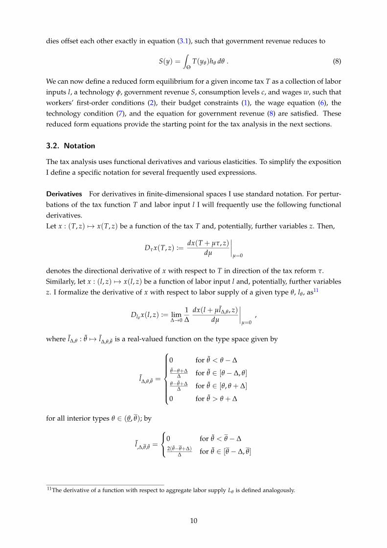
dies offset each other exactly in equation (3.1), such that government revenue reduces to

S(y) =∫

ΘT(yθ)hθ dθ . (8)

We can now define a reduced form equilibrium for a given income tax T as a collection of laborinputs l, a technology φ, government revenue S, consumption levels c, and wages w, such thatworkers’ first-order conditions (2), their budget constraints (1), the wage equation (6), thetechnology condition (7), and the equation for government revenue (8) are satisfied. Thesereduced form equations provide the starting point for the tax analysis in the next sections.

3.2. Notation

The tax analysis uses functional derivatives and various elasticities. To simplify the expositionI define a specific notation for several frequently used expressions.

Derivatives For derivatives in finite-dimensional spaces I use standard notation. For pertur-bations of the tax function T and labor input l I will frequently use the following functionalderivatives.Let x : (T, z) 7→ x(T, z) be a function of the tax T and, potentially, further variables z. Then,

Dτx(T, z) :=dx(T + µτ, z)

dµ

∣∣∣∣µ=0

denotes the directional derivative of x with respect to T in direction of the tax reform τ.Similarly, let x : (l, z) 7→ x(l, z) be a function of labor input l and, potentially, further variablesz. I formalize the derivative of x with respect to labor supply of a given type θ, lθ , as11

Dlθ x(l, z) := lim∆→0

1∆

dx(l + µl∆,θ , z)dµ

∣∣∣∣µ=0

,

where l∆,θ : θ 7→ l∆,θ,θ is a real-valued function on the type space given by

l∆,θ,θ =

0 for θ < θ − ∆θ−θ+∆

∆ for θ ∈ [θ − ∆, θ]

θ−θ+∆∆ for θ ∈ [θ, θ + ∆]

0 for θ > θ + ∆

for all interior types θ ∈ (θ, θ); by

l,∆,θ,θ =

0 for θ < θ − ∆2(θ−θ+∆)

∆ for θ ∈ [θ − ∆, θ]

11The derivative of a function with respect to aggregate labor supply Lθ is defined analogously.

10

for the highest type θ; and by

l∆,θ,θ =

2(θ−θ+∆)

∆ for θ ∈ [θ, θ + ∆]

0 for θ > θ + ∆

for the lowest type θ. Intuitively, the derivative is obtained by perturbing the labor supplyfunction in a continuous way in a neighborhood of type θ and letting this neighborhoodconverge to θ. Appendix A.1 demonstrates that the thus defined derivative works in a naturalway by showing in detail that

DLθ

∫ θ

θwθ Lθ dθ = wθ ∀θ .

This also proves the labor demand equation (3.1).The tax analysis below often distinguishes between the direct effect of changes in T or l onan outcome x and the indirect effect mediated through the response of technology φ∗. Inparticular, suppose x : (T, φ) 7→ x(T, φ) depends (directly) on taxes T and technology φ. Thedirect effect of a tax reform in direction τ, holding technology fixed, is then given by Dτx(T, φ)

as defined above. For the indirect effect of the tax reform via technology (the induced technicalchange effect, henceforth) I introduce the following notation:

Dφ,τx(T, φ∗(T)) :=dx(T, φ∗(T + µτ))

dµ

∣∣∣∣µ=0

.

Here, φ∗(T) denotes the equilibrium technology at tax function T. The total effect of thereform on x is then obtained as the sum of the direct and the induced technical change effect.Writing x∗(T) := x(T, φ∗(T)), we get

Dτx∗(T) = Dτx(T, φ∗(T)) + Dφ,τx(T, φ∗(T)) .

Analogously, if x : (l, φ) 7→ x(l, φ) is a function of labor input l and technology φ, the inducedtechnical change effect of a labor input change in direction lθ is

Dφ,lθ = lim∆→0

1∆

dx(l, φ∗(l + µl∆,θ)

dµ

∣∣∣∣µ=0

,

where φ∗(l) is given by equation (7).

Wage Elasticities The response of wages to labor input changes plays a central role in thetax analysis. Consider wages as given by (6), that is, for each type θ the wage wθ is a functionof labor inputs l and technology φ.The first set of wage elasticities is concerned with the direct effect of labor inputs on wages,holding technology constant. I call these elasticities the within-technology substitution elas-ticities (sometimes just substitution elasticities, for brevity), as they describe the changes inmarginal productivities induced by factor substitution within a given technology. The own-

11

wage substitution elasticity, that is, the elasticity of wθ with respect to lθ , is defined as

γθ,θ :=lθ

wθlim∆→0

dwθ(l + µl∆,θ , φ)

dµ

∣∣∣∣µ=0

.

Alternatively, we could write the wage wθ as a function of φ, l, and type θ’s labor input lθ

separately, as typically a type’s labor input affects its own wage in a way distinct from thelabor input function l (see for example the CES case in Section 3.4). Then, the own-wagesubstitution elasticity is simply

γθ,θ =lθ

wθ

∂wθ(lθ , l, φ)

∂lθ.

The cross-wage substitution elasticity, that is, the elasticity of wθ with respect to a differenttype’s labor input lθ (with θ 6= θ), is given by

γθ,θ :=lθ

wθDlθ wθ(l, φ) ,

with the derivative Dlθ as defined above.The second set of wage elasticities captures the induced technical change effects of changesin labor inputs on wages. These elasticities are called the technical change elasticities in thefollowing. The own-wage technical change elasticity is defined as

ρθ,θ :=lθ

wθlim∆→0

dwθ(l, φ∗(l + µl∆,θ))

dµ

∣∣∣∣µ=0

.

Again, the CES case in Section 3.4 clarifies why this is a natural definition of the own-wagetechnical change elasticity and how it can be expressed in terms of conventional partial deriva-tives.The cross-wage technical change elasticity measures how wage wθ is affected by a change inanother type’s labor supply lθ via induced technical change. Formally, it is given by

ρθ,θ :=lθ

wθDφ,lθ wθ(l, φ∗(l)) ,

where the derivative Dφ,lθ has been defined above.

Rate of Progressivity The rate of progressivity of a tax schedule T is defined as minus theelasticity of the marginal retention rate R′T with respect to income,

PT(y) := −R′′T(y)yR′T(y)

.

It measures the progression of marginal tax rates as income increases. If the income tax islinear such that marginal tax rates are constant, PT(y) is zero. If the income tax is progressive(regressive) in the sense that marginal tax rates increase (decrease) with income, the rate ofprogressivity is positive (negative).

12

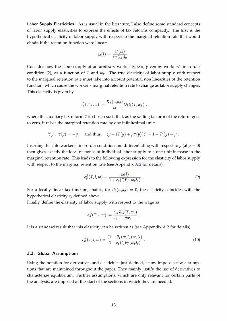
Labor Supply Elasticities As is usual in the literature, I also define some standard conceptsof labor supply elasticities to express the effects of tax reforms compactly. The first is thehypothetical elasticity of labor supply with respect to the marginal retention rate that wouldobtain if the retention function were linear:

eθ(l) :=v′(lθ)

v′′(lθ)lθ.

Consider now the labor supply of an arbitrary worker type θ, given by workers’ first-ordercondition (2), as a function of T and wθ . The true elasticity of labor supply with respectto the marginal retention rate must take into account potential non linearities of the retentionfunction, which cause the worker’s marginal retention rate to change as labor supply changes.This elasticity is given by

εRθ (T, l, w) :=

R′T(wθ lθ)

lθDτ lθ(T, wθ) ,

where the auxiliary tax reform τ is chosen such that, as the scaling factor µ of the reform goesto zero, it raises the marginal retention rate by one infinitesimal unit:

∀ y : τ(y) = −y , and thus: (y− (T(y) + µτ(y)))′ = 1− T′(y) + µ .

Inserting this into workers’ first-order condition and differentiating with respect to µ (at µ = 0)then gives exactly the local response of individual labor supply to a one unit increase in themarginal retention rate. This leads to the following expression for the elasticity of labor supplywith respect to the marginal retention rate (see Appendix A.2 for details):

εRθ (T, l, w) =

eθ(l)1 + eθ(l)PT(wθ lθ)

. (9)

For a locally linear tax function, that is, for PT(wθ lθ) = 0, the elasticity coincides with thehypothetical elasticity eθ defined above.Finally, define the elasticity of labor supply with respect to the wage as

εwθ (T, l, w) :=

wθ

lθ

∂lθ(T, wθ)

∂wθ.

It is a standard result that this elasticity can be written as (see Appendix A.2 for details)

εwθ (T, l, w) =

(1− PT(wθ lθ))eθ(l)1 + eθ(l)PT(wθ lθ)

. (10)

3.3. Global Assumptions

Using the notation for derivatives and elasticities just defined, I now impose a few assump-tions that are maintained throughout the paper. They mainly justify the use of derivatives tocharacterize equilibrium. Further assumptions, which are only relevant for certain parts ofthe analysis, are imposed at the start of the sections in which they are needed.

13

I impose the assumptions directly on the parameters of the reduced form equations. They canof course be mapped into assumptions on the fundamentals of the specific model presentedabove. I decide to impose them on the reduced form because this seems more transparentand, as argued before, the reduced form is far more general than the model itself.

Assumption 1. The parameters of the reduced form equations (2), (1), (6), (7), and (8) satisfy thefollowing.

1. The derivative Dlθ F exists and is strictly positive for all θ.

2. The wage elasticities γθ,θ and ρθ,θ exist for all θ, θ.

3. The density h is C1 and strictly positive for all θ.

4. The maximizer argmaxφ∈Φ F(l, φ) exists and is unique for all l.

5. The disutility of labor v is C2 with v′ > 0 and v′′ > 0 everywhere.

6. Whenever an exogenous tax T is considered, it is C2 and satisfies T′ < 1 everywhere.

The first two points say that the aggregate production function F is twice differentiable underthe differentiation operator Dlθ . Together with the third point (especially h > 0 everywhere),they ensure that wages and wage elasticities are always well defined. The fourth point impliesthat the equilibrium technology φ∗(l) is unique for any equilibrium labor input l. This allowsme to write results in terms of equilibrium values instead of sets of equilibrium values. Thelatter would complicate the notation without adding interesting substance. Finally, the differ-entiability assumptions on v and T ensure that the labor supply elasticity eθ and the rate ofprogressivity of the tax schedule are well defined.

3.4. Special Cases

Parts of the results of the tax analysis require further structural assumptions on productionfunctions, utility functions, or the tax function. I introduce these special cases here and referto them in the tax analysis whenever needed.

CES Production An important special case of the model is obtained when the aggregateproduction function F features a constant elasticity of substitution (CES) between workertypes while the research cost functions are iso elastic. I refer to this configuration of themodel as the CES case.The CES case is obtained via the following assumptions on the fundamentals of the modelpresented above.

G(L, φ, q) =

[∫ θ

θ

(κθ L1−α

θ

∫ 1

0φθ,kqα

θ,k dk) σ−1

σ

dθ

] σσ−1

Cθ(φθ,k) = φδθ,k .

14

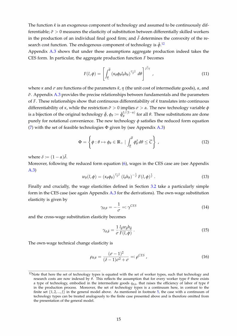
The function κ is an exogenous component of technology and assumed to be continuously dif-ferentiable; σ > 0 measures the elasticity of substitution between differentially skilled workersin the production of an individual final good firm; and δ determines the convexity of the re-search cost function. The endogenous component of technology is φ.12

Appendix A.3 shows that under these assumptions aggregate production indeed takes theCES form. In particular, the aggregate production function F becomes

F(l, φ) =

[∫ θ

θ(κθφθ lθhθ)

σ−1σ dθ

] σσ−1

, (11)

where κ and σ are functions of the parameters κ, η (the unit cost of intermediate goods), α, andσ. Appendix A.3 provides the precise relationships between fundamentals and the parametersof F. These relationships show that continuous differentiability of κ translates into continuousdifferentiability of κ, while the restriction σ > 0 implies σ > α. The new technology variable φ

is a bijection of the original technology φ, φθ := φ1/(1−α)θ for all θ. These substitutions are done

purely for notational convenience. The new technology φ satisfies the reduced form equation(7) with the set of feasible technologies Φ given by (see Appendix A.3)

Φ =

{φ : θ 7→ φθ ∈ R+ |

∫ θ

θφδ

θ dθ ≤ C

}, (12)

where δ := (1− α)δ.Moreover, following the reduced form equation (6), wages in the CES case are (see AppendixA.3)

wθ(l, φ) = (κθφθ)σ−1

σ (lθhθ)− 1

σ F(l, φ)1σ . (13)

Finally and crucially, the wage elasticities defined in Section 3.2 take a particularly simpleform in the CES case (see again Appendix A.3 for the derivations). The own-wage substitutionelasticity is given by

γθ,θ = −1σ=: γCES (14)

and the cross-wage substitution elasticity becomes

γθ,θ =1σ

lθwθhθ

F(l, φ). (15)

The own-wage technical change elasticity is

ρθ,θ =(σ− 1)2

(δ− 1)σ2 + σ=: ρCES , (16)

12Note that here the set of technology types is equated with the set of worker types, such that technology andresearch costs are now indexed by θ. This reflects the assumption that for every worker type θ there existsa type of technology, embodied in the intermediate goods qθ,k, that raises the efficiency of labor of type θin the production process. Moreover, the set of technology types is a continuum here, in contrast to thefinite set {1, 2, ..., J} in the general model above. As mentioned in footnote 5, the case with a continuum oftechnology types can be treated analogously to the finite case presented above and is therefore omitted fromthe presentation of the general model.

15

and the cross-wage technical change elasticity is given by

ρθ,θ = −(σ− 1)2

(δ− 1)σ2 + σ

lθwθhθ

F(l, φ). (17)

Iso-Elastic Disutility of Labor When the disutility of labor is iso elastic, workers’ utilityfunctions take the form

uθ = cθ −e

e + 1l

e+1e

θ .

In this case, the hypothetical labor supply elasticity eθ(l) is constant across θ and l:

eθ(l) = e for all θ, l. .

Constant-Rate-of-Progressivity Taxes A constant-rate-of-progressivity (CRP) tax functiontakes the form (e.g. Feldstein, 1969; Heathcote, Storesletten and Violante, 2017)

T(y) = y− λy1−P .

For any CRP tax schedule T the rate of progressivity PT is constant across income levels:

PT(y) = P for all y .

This special case, when combined with iso-elastic disutility of labor, ensures that the laborsupply elasticities εR

θ and εwθ are constant in θ.

The combination of iso-elastic disutility of labor and CRP tax schedules plays an importantrole in simplifying and clarifying the results of the tax analysis by suppressing heterogeneityin labor supply responses to changes in marginal tax rates.

4. Directed Technical Change

Income tax reforms affect technical change via differential changes in labor supply acrossworker types. An important building block of the tax analysis below is therefore the relation-ship between the structure of labor supply and technical change. This relationship is studiedby the theory of directed technical change.To review the central results (for the purpose of the tax analysis below) of this theory, takelabor supply l as exogenous for the moment and consider wages and equilibrium technologyas determined by the reduced form equations (6) and (7) given labor inputs (copied here forthe reader’s convenience):

wθ(l, φ) =1hθ

Dlθ F(l, φ)

φ∗(l) := argmaxφ∈Φ

F(l, φ) .

16

4.1. Weak Relative Bias

Starting from the previous two equations, a first major results of directed technical changetheory identifies conditions under which any increase in the relative supply of skill in theeconomy induces skill-biased technical change.In particular, let dl be a change in the labor input l. We say that dl is an increase in therelative supply of skill if it raises the supply of more skilled relative to the supply of lessskilled workers, that is, dlθ/lθ increases in θ. Similarly, a technology φ is skill-biased relativeto another technology φ if more skilled workers earn higher wages relative to less skilledworkers under φ than under φ, that is, wθ(l, φ)/wθ(l, φ) ≥ wθ(l, φ)/wθ(l, φ) for all θ ≥ θ andall l. In this case we write φ � φ.For any increase in relative skill supply to induce skill-biased technical change, I have shownin previous work that the following non-parametric restrictions on the aggregate productionfunction F are sufficient and close to necessary (Loebbing, 2018).

Assumption 2. The aggregate production function F is homogeneous in l and quasisupermodular inφ.

Homogeneity of F in labor is in fact already implied by the structure of the model presented inSection 3.1, so it imposes no further restrictions (see Appendix A.4). By quasisupermodularityI mean the following here. For any l and any two technologies φ and φ, if F(l, φ) ≤ F(l, φ) forall φ � φ, φ, then there must exist a φ � φ, φ such that F(l, φ) ≥ F(l, φ).13

For two technologies that can are ordered according to their skill-bias, the condition is notrestrictive. So, to understand the restrictions involved, suppose that neither φ � φ nor φ � φ.For illustration, consider a setting with three different types and let φ induce a higher skillpremium at the top (i.e., between the high and the middle skill) while φ induces a higherskill premium at the bottom (i.e., between the middle and the low skill). Moreover, supposethat moving from any technology φ that induces lower skill premia than both φ and φ toφ increases output. Note that such a technical change raises the skill premium at the top.Quasisupermodularity then says that there must also be a technical change starting from φ

that raises the skill premium at the top and increases output. In short, if we can raise outputby an increase in the skill premium at the top when starting from low skill premia everywhere,then we must also be able to raise output by an increase in the skill premium at the top whenthe skill premium at the bottom is already elevated.More generally, this implies that technical changes that increase inequality on different seg-ments of the wage distribution must not be substitutes: technical change that raises inequalityon some segment must not reduce the profitability of technical change raising inequality onanother segment. The CES case introduced in Section 3.4 is exactly the case where technical

13Note that this slightly deviates from the original definition of quasisupermodularity given by Milgrom andShannon (1994). For their definition, we would first have to assume that the set (Φ,�) has a lattice structure,that is, for any two technologies φ and φ there exist supremum and infimum in Φ. Then, quasisupermodularitywould be defined using infimum and supremum instead of arbitrary technologies below and above φ andφ. In particular, for any l and any φ, φ, if F(l, φ) ≤ F(l, φ), then F(l, φ) ≥ F(l, φ), where φ and φ denoteinfimum and supremum of φ and φ. My definition is slightly less restrictive (and sufficiently restrictive for thepresent purpose), but more importantly it does not require to introduce the lattice structure of Φ, which wouldunnecessarily complicate the exposition.

17

changes affecting different parts of the wage distribution are independent of each other: theprofitability of increasing productivity of some worker type θ at the cost of reducing produc-tivity for some other type θ only depends on productivity and labor input levels of these twotypes, but not on the productivity distribution over other types of workers.14

In the absence of precise empirical evidence about the complementarity relationships betweendifferent forms of technical change, the agnostic view (neither strict complementarity nor strictsubstitutability) of the CES function seems a reasonable benchmark. Note also that, while Iam not aware of empirical tests of quasisupermodularity in the aggregate production process,the implications of quasisupermodularity presented in Lemma 1 below receive support in theempirical literature. I discuss this literature in Section 7, when quantifying the results of thetax analysis.15

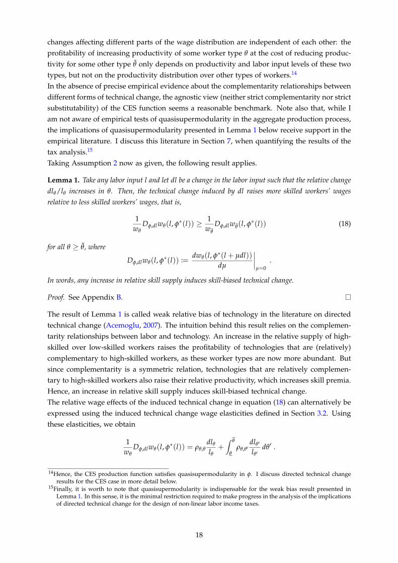
Taking Assumption 2 now as given, the following result applies.

Lemma 1. Take any labor input l and let dl be a change in the labor input such that the relative changedlθ/lθ increases in θ. Then, the technical change induced by dl raises more skilled workers’ wagesrelative to less skilled workers’ wages, that is,

1wθ

Dφ,dlwθ(l, φ∗(l)) ≥ 1wθ

Dφ,dlwθ(l, φ∗(l)) (18)

for all θ ≥ θ, where

Dφ,dlwθ(l, φ∗(l)) :=dwθ(l, φ∗(l + µdl))

dµ

∣∣∣∣µ=0

.

In words, any increase in relative skill supply induces skill-biased technical change.

Proof. See Appendix B.

The result of Lemma 1 is called weak relative bias of technology in the literature on directedtechnical change (Acemoglu, 2007). The intuition behind this result relies on the complemen-tarity relationships between labor and technology. An increase in the relative supply of high-skilled over low-skilled workers raises the profitability of technologies that are (relatively)complementary to high-skilled workers, as these worker types are now more abundant. Butsince complementarity is a symmetric relation, technologies that are relatively complemen-tary to high-skilled workers also raise their relative productivity, which increases skill premia.Hence, an increase in relative skill supply induces skill-biased technical change.The relative wage effects of the induced technical change in equation (18) can alternatively beexpressed using the induced technical change wage elasticities defined in Section 3.2. Usingthese elasticities, we obtain

1wθ

Dφ,dlwθ(l, φ∗(l)) = ρθ,θdlθ

lθ+∫ θ

θρθ,θ′

dlθ′

lθ′dθ′ .

14Hence, the CES production function satisfies quasisupermodularity in φ. I discuss directed technical changeresults for the CES case in more detail below.

15Finally, it is worth to note that quasisupermodularity is indispensable for the weak bias result presented inLemma 1. In this sense, it is the minimal restriction required to make progress in the analysis of the implicationsof directed technical change for the design of non-linear labor income taxes.

18

This expression offers an easy way to verify the statement of Lemma 1 for the CES case. Inparticular, consider the difference

ρθ,θdlθ

lθ+∫ θ

θρθ,θ′

dlθ′

lθ′dθ′ − ρθ,θ

dlθ

lθ

−∫ θ

θρθ,θ′

dlθ′

lθ′dθ′

for some types θ ≥ θ. Using equations (16) and (17), which specify the induced technicalchange elasticities in the CES case, this difference becomes

ρCES(

dlθ

lθ− dlθ

lθ

),

which is clearly positive whenever dlθ/lθ increases in θ. Hence, if dl is an increase in relativeskill supply, the induced technical change raises more skilled workers’ wages relative to thewages of less skilled workers, which is the statement of Lemma 1.

4.2. Strong Relative Bias

The weak bias results only concern the effects of labor supply changes on wages mediatedby induced technical change. These effects are important to identify precisely what is addedby accounting for directed technical change. Yet in general, wages are also affected by factorsubstitution within a given technology, that is, by the within-technology substitution effectsdescribed in Section 3.2. These work typically against the induced technical change effects,reducing skill premia when relative skill supply rises and increasing them otherwise. Animportant question is then whether the induced technical change effects are strong enough tooutweigh the effects coming from within-technology factor substitution, or vice versa.The strong bias results of directed technical change theory provide an answer to this question.The theory says that there is strong relative bias of technology if the induced technical changeeffects dominate the within-technology substitution effects, such that the total effect of anincrease in relative skill supply is to raise skill premia. In Loebbing (2018), I show that strongrelative bias can occur if the production function fails to be quasisconcave. Quasiconvexityin aggregate production can in turn be microfounded by models with imperfect competition,Arrow (1962) type external effects between firms, or endogenous firm entry and inframarginalrents (Acemoglu, 2007; Loebbing, 2018). The model presented in Section 3.1 features imperfectcompetition on technology markets. So strong bias is a possibility.For the CES case, there is an exact parametric condition for strong bias. In particular, the totaleffect of a labor supply change dl on the relative wage between types θ ≥ θ is

(ρθ,θ + γθ,θ)dlθ

lθ+∫ θ

θ(ρθ,θ′ + γθ,θ′)

dlθ′

lθ′dθ′ − (ρθ,θ + γθ,θ)

dlθ

lθ

−∫ θ

θ(ρθ,θ′ + γθ,θ′)

dlθ′

lθ′dθ′

= (ρCES + γCES)

(dlθ

lθ− dlθ

lθ

).

Considering again an increase in the relative input of more skilled workers, dl such that

19

dlθ/lθ ≥ dlθ/lθ , the effect on the relative wage is positive if and only if

ρCES + γCES ≥ 0 . (19)

Hence, if condition (19) is satisfied, induced technical change effects dominate substitutioneffects and the total effect of an increase in relative skill supply on skill premia is positive.

5. Tax Reforms

Starting from a given tax T, a tax reform is represented by the change from T to T + µτ, whereµ ∈ R+ and τ : y 7→ τ(y) ∈ R is a C2 real-valued function. In this notation, µ is the scalingfactor of the tax reform while τ indicates its direction: If τ(y) is positive (negative) at someincome level y, the reform raises (lowers) the tax burden for workers who earn y.The curvature of τ, relative to the curvature of T, governs the progressivity of the reform.More precisely, I call a reform progressive if the post-reform tax schedule has a higher rate ofprogressivity than the pre-reform schedule everywhere.

Definition 1. Starting from tax T the tax reform (τ, µ) is progressive if and only if

PT(y) ≥ PT(y) ∀ y ,

where T := T + µτ denotes the post-reform tax function.

This definition is equivalent to the following characterizations of progressivity.

Lemma 2. Take any tax function T. The following statements are equivalent.

1. The reform (τ, µ) is progressive according to Definition 1.

2. The post-reform tax T = T + µτ can be obtained by taxing post-tax income under the initial taxin a progressive way, that is, by means of a tax function with increasing marginal tax rates:

RT = r ◦ RT

for some concave function r.

3. The reform (τ, µ) satisfies

τ′(y)1− T′(y)

≥ τ′(y)1− T′(y)

∀ y ≥ y .

Proof. See Appendix C.

The first equivalence provides an intuitive interpretation of progressivity: a reform is progres-sive if and only if it can be obtained by augmenting the initial tax by an additional tax onpost-tax income that features increasing marginal tax rates. In this sense, a progressive reformis obtained by taxing the initial post-tax income in a progressive way.

20

The second equivalence shows that a progressive reform raises the marginal tax rate relative tothe initial marginal retention rate by more for higher incomes. Alternatively, the marginal re-tention rate for higher incomes is reduced relative to that for lower incomes. This equivalencewill turn out useful in the analysis below.In the following I focus on the local effects of a reform in the direction of τ, that is, theeffects on economic outcomes of changing T to T + µτ as µ → 0. Note that this does notlead to confusion with the definition of progressivity, because, as indicated by the secondequivalence in Lemma 2, Definition 1 only depends on the direction τ of a reform but noton the scaling factor µ. Moreover, I assume without loss of generality that worker types areordered according to their wages under the initial tax schedule, that is, wθ ≤ wθ if θ ≤ θ underthe initial tax.To describe the effects of tax reforms on economic outcomes formally, I write equilibriumvariables as a function of the tax, that is, the equilibrium value of a variable x (e.g. wages orlabor inputs) under tax T is denoted by x(T).16

5.1. Direction of Induced Technical Change

A key step in the analysis of the effects of tax reforms is to characterize the responses of laborinputs to a given reform. Let

lθ,τ(T) :=1lθ

Dτ lθ(T)

denote the relative change in the labor input of type θ in response to reform τ. The relativelabor input changes must satisfy the following fixed point equation (see Appendix C.1 fordetails).17

lθ,τ(T) = −εRθ

τ′(yθ(T))1− T′(yθ(T))

+ εwθ (γθ,θ + ρθ,θ)lθ,τ(T) + εw

θ

∫ θ

θ(γθ,θ + ρθ,θ)lθ,τ dθ . (20)

In equilibrium, labor inputs respond directly to the tax reform (the first term in equation(20)) but they also cause wages to adjust. These wage adjustments in turn feed back to laborinputs, which is captured by the second and third terms in equation (20). Accounting forthese feedback effects gives rise to the fixed point character of equation (20).I solve for the fixed point of equation (20) by an iteration procedure. Within the iteration stepsI disentangle the feedback effects purely transmitted via induced technical change from thosetransmitted via within-technology factor substitution. Thereby, I obtain a decomposition ofthe total labor input response into a substitution and an induced technical change component.The slope of the induced technical change component over the type space can then be signedfor the case of a progressive tax reform, using the structure of the induced technical changeeffects predicted by the theory of directed technical change.18

16Note that in some cases this involves an abuse of notation. I write for example wθ(l, φ) in equation (6) to denotewages as a function of labor inputs and technology; now I use wθ(T, φ∗(T)) to denote wages as a function ofthe tax. The latter is meant as a short cut for wθ(l(T), φ∗(l(T))), where l(T) denotes labor inputs under tax T.

17All elasticities in this section are evaluated at the equilibrium under the initial tax T. I do not write thisdependence explicitly to save on notation.

18The expression for labor input responses in Lemma 3 differs from that provided by Sachs et al. (2019) evenwhen ignoring induced technical change effects and the ensuing decomposition of the total effect (i.e., when

21

Lemma 3. Fix an initial tax T and suppose that workers’ second-order conditions hold strictly underT such that the labor supply elasticities εR

θ and εwθ are well defined (see Appendix A.2). Moreover,

suppose that under T,

supθ∈Θ

[(εw

θ ρθ,θ)2]+ ∫ θ

θ

∫ θ

θ(εw

θ ρθ,θ)2 dθ dθ + 2

√∫ θ

θ

∫ θ

θ

(εw

θ ρθ,θεwθ ρθ,θ

)2 dθ dθ < 1 (21)

supθ∈Θ

[(εw

θ ζθ,θ)2]+ ∫ θ

θ

∫ θ

θ(εw

θ ζθ,θ)2 dθ dθ + 2

√∫ θ

θ

∫ θ

θ

(εw

θ ζθ,θεwθ ζθ,θ

)2 dθ dθ < 1 , (22)

where ζθ,θ := γθ,θ + ρθ,θ .19

Then, the effect of tax reform τ on the labor input of type θ can be written as

lθ,τ(T) =∞

∑n=0

l(n)θ,τ (T) (23)

for all θ ∈ Θ, where

l(0)θ,τ (T) = −εRθ

τ′(yθ(T))1− T′(yθ(T))

l(n)θ,τ (T) = εwθ ζθ,θ l(n−1)

θ,τ (T) + εwθ

∫ θ

θζθ,θ l(n−1)

θ,τ(T) dθ ∀ n > 0 .

The total effect on labor inputs can be decomposed as follows,

lθ,τ(T) = −εRθ

τ′(yθ(T))1− T′(yθ(T))

+∞

∑n=1

TE(n)θ,τ (T)︸ ︷︷ ︸

=:TEθ,τ(T)

+∞

∑n=1

SE(n)θ,τ (T)︸ ︷︷ ︸

=:SEθ,τ(T)

, (24)

where (omitting the argument T)

TE(1)θ,τ =εw

θ ρθ,θ(−εRθ )

τ′(yθ(T))1− T′(yθ(T))

+ εwθ

∫ θ

θρθ,θ(−εR

θ)

τ′(yθ(T))1− T′(yθ(T))

dθ

TE(n)θ,τ =εw

θ ρθ,θ TE(n−1)θ,τ + εw

θ

∫ θ

θρθ,θ TE(n−1)

θ,τ dθ ∀ n > 1

SE(1)θ,τ =εw

θ γθ,θ(−εRθ )

τ′(yθ(T))1− T′(yθ(T))

+ εwθ

∫ θ

θγθ,θ(−εR

θ)

τ′(yθ(T))1− T′(yθ(T))

dθ

SE(n)θ,τ =εw

θ γθ,θ(TE(n−1)θ,τ + SE(n−1)

θ,τ ) + ρθ,θ SE(n−1)θ,τ

+ εwθ

∫ θ

θ

[γθ,θ(TE(n−1)

θ,τ + SE(n−1)θ,τ ) + ρθ,θ SE(n−1)

θ,τ

]dθ ∀ n > 1 .

setting ρθ,θ = 0 for all θ, θ). I discuss the relationship between Lemma 3 and the results of Sachs et al. (2019) inAppendix C.4. In short, my approach has the advantage that, after decomposing the total effect, it allows meto derive analytical insights into the structure of the induced technical change component.

19Conditions (21) and (22) ensure that the series in equations (23) and (24) converge. They are sufficient butgenerally not necessary for convergence. If the conditions are not satisfied, the equilibrium may be unstable inthe sense that an increase in some types’ labor inputs may trigger a wage adjustment that is more than sufficientto justify the initial increase in labor inputs. I check that the conditions are satisfied in the quantitative analysis.

22

If εwθ is constant in θ (e.g. because the disutility of labor is iso elastic and T is CRP), then TEθ,τ is

decreasing in θ if εRθ τ′(yθ(T))/(1− T′(yθ(T))) increases in θ.

Hence, if εRθ is also constant in θ, TEθ,τ decreases in θ for any progressive reform τ.

Proof. See Appendix C.1.

Equation (23) expresses the labor input change induced by reform τ as the sum over successiverounds of general equilibrium adjustments, capturing feedback loops from labor supply towages and back to labor supply. The first summand l(0)θ,τ (T) is the direct effect of the reform onlabor supply, holding wages constant. The direct adjustment of labor supply in turn changeswages, which then feeds back into labor supply. This first-round feedback effect is capturedby l(1)θ,τ (T). The labor supply change l(1)θ,τ (T) then induces another adjustment of wages, whichagain affects labor supply, and so on.20

Equation (24) decomposes the total labor input change into three components. The first isthe direct effect of reform τ, holding wages constant. The second term isolates the partof the general equilibrium feedback in which the effect of labor supply on wages is purelytransmitted via induced technical change. The third term collects the remaining parts of thefeedback, containing within-technology substitution effects from labor supply on wages.With constant labor supply elasticities across workers, the induced technical change compo-nent TEθ,τ(T) is decreasing in θ for any progressive tax reform; that is, the induced technicalchange component reduces the labor supply of more relative to less skilled workers. This fol-lows from the weak bias result of directed technical change theory. Intuitively, with constantlabor supply elasticities, the direct effect of a progressive tax reform on labor supply is toreduce relative skill supply. By weak bias, this induces technical change reducing skill premia(equalizing technical change, henceforth). Again under constant labor supply elasticities, suchequalizing technical change feeds back into a further reduction in relative skill supply, whichin turn induces further equalizing technical change. Summing over the thus induced roundsof reductions in relative skill supply eventually gives rise to the term TEθ,τ(T), which mustthen also reduce relative skill supply (i.e., decrease in θ).We can now use Lemma 3 to study the effects of tax reforms on technical change. More pre-cisely, consider the relative changes in wages that are caused by the technical change inducedby a reform τ. Using the derivative Dφ,τ introduced in Section 3.2, these relative wage changesare given by

1wθ

Dφ,τwθ(T, φ∗(T)) .

They can be expressed in terms of induced technical change elasticities and labor input re-sponses as follows.

1wθ

Dφ,τwθ(T, φ∗(T)) = ρθ,θ lθ,τ(T) +∫ θ

θρθ,θ lθ,τ(T) dθ . (25)

20Mathematically, the series representation in equation (23) is the von Neumann series expansion of the solution tothe fixed point equation (20). In particular, the fixed point equation can be written abstractly as (I − X)lτ = Z,where I denotes the identity function, X is a linear operator on the space of real-valued functions on Θ, andZ is the direct effect of τ on labor supply. Inverting I − X yields lτ = (I − X)−1Z. By von Neumann seriesexpansion, this is equivalent to lτ = ∑∞

n=0 XnZ.

23

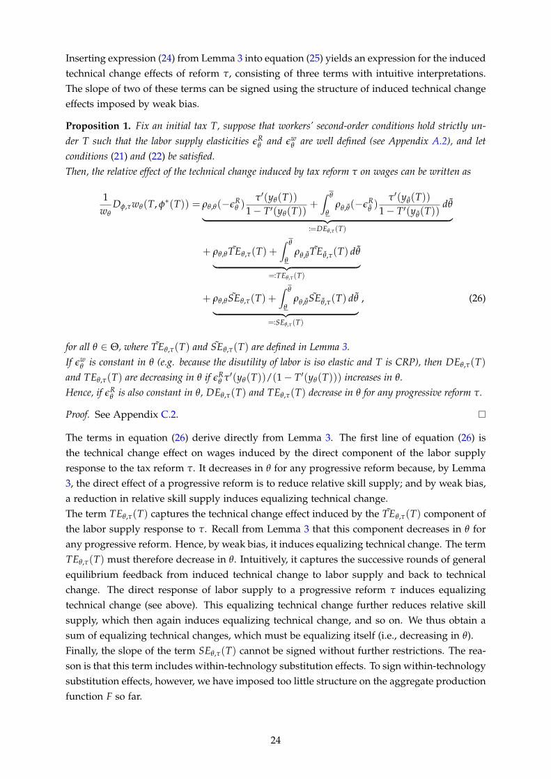
Inserting expression (24) from Lemma 3 into equation (25) yields an expression for the inducedtechnical change effects of reform τ, consisting of three terms with intuitive interpretations.The slope of two of these terms can be signed using the structure of induced technical changeeffects imposed by weak bias.

Proposition 1. Fix an initial tax T, suppose that workers’ second-order conditions hold strictly un-der T such that the labor supply elasticities εR

θ and εwθ are well defined (see Appendix A.2), and let

conditions (21) and (22) be satisfied.Then, the relative effect of the technical change induced by tax reform τ on wages can be written as

1wθ

Dφ,τwθ(T, φ∗(T)) = ρθ,θ(−εRθ )

τ′(yθ(T))1− T′(yθ(T))

+∫ θ

θρθ,θ(−εR

θ)

τ′(yθ(T))1− T′(yθ(T))

dθ︸ ︷︷ ︸:=DEθ,τ(T)

+ ρθ,θ TEθ,τ(T) +∫ θ

θρθ,θ TEθ,τ(T) dθ︸ ︷︷ ︸

=:TEθ,τ(T)

+ ρθ,θ SEθ,τ(T) +∫ θ

θρθ,θ SEθ,τ(T) dθ︸ ︷︷ ︸

=:SEθ,τ(T)

, (26)

for all θ ∈ Θ, where TEθ,τ(T) and SEθ,τ(T) are defined in Lemma 3.If εw

θ is constant in θ (e.g. because the disutility of labor is iso elastic and T is CRP), then DEθ,τ(T)and TEθ,τ(T) are decreasing in θ if εR

θ τ′(yθ(T))/(1− T′(yθ(T))) increases in θ.Hence, if εR

θ is also constant in θ, DEθ,τ(T) and TEθ,τ(T) decrease in θ for any progressive reform τ.

Proof. See Appendix C.2.

The terms in equation (26) derive directly from Lemma 3. The first line of equation (26) isthe technical change effect on wages induced by the direct component of the labor supplyresponse to the tax reform τ. It decreases in θ for any progressive reform because, by Lemma3, the direct effect of a progressive reform is to reduce relative skill supply; and by weak bias,a reduction in relative skill supply induces equalizing technical change.The term TEθ,τ(T) captures the technical change effect induced by the TEθ,τ(T) component ofthe labor supply response to τ. Recall from Lemma 3 that this component decreases in θ forany progressive reform. Hence, by weak bias, it induces equalizing technical change. The termTEθ,τ(T) must therefore decrease in θ. Intuitively, it captures the successive rounds of generalequilibrium feedback from induced technical change to labor supply and back to technicalchange. The direct response of labor supply to a progressive reform τ induces equalizingtechnical change (see above). This equalizing technical change further reduces relative skillsupply, which then again induces equalizing technical change, and so on. We thus obtain asum of equalizing technical changes, which must be equalizing itself (i.e., decreasing in θ).Finally, the slope of the term SEθ,τ(T) cannot be signed without further restrictions. The rea-son is that this term includes within-technology substitution effects. To sign within-technologysubstitution effects, however, we have imposed too little structure on the aggregate productionfunction F so far.

24

Since we cannot sign the slope of the term SEθ,τ(T), we can also not sign the total inducedtechnical change effect of a progressive tax reform on relative wages. To do so, additionalrestrictions are needed. The most radical approach is to restrict the aggregate productionfunction F to be linear in l for any technology φ. Then, there are no within-technology sub-stitution effects. The only remaining are the direct effect and the feedback effects via inducedtechnical change, both of which compress the wage distribution.

Corollary 1. Fix an initial tax T, suppose that workers’ second-order conditions hold strictly under Tsuch that the labor supply elasticities εR

θ and εwθ are well defined (see Appendix A.2), and let condition

(21) be satisfied. In addition, suppose that aggregate production F is linear in l such that γθ,θ = 0 forall θ, θ. Then, SEθ,τ(T) = 0.Moreover, if εw

θ and εRθ are constant across types (e.g. because the disutility of labor is iso-elastic and T

is CRP), any progressive tax reform induces technical change that reduces all skill premia.

Proof. If γθ,θ = 0 for all θ, θ, conditions (21) and (22) are identical, so the conditions of Propo-sition 1 are satisfied. The definition of SEθ,τ then immediately implies SEθ,τ = 0. The last partof Corollary 1 also follows directly from Proposition 1.

A similarly clear pattern emerges when we assume that aggregate production takes the CESform introduced in Section 3.4. In that case the wage elasticities γθ,θ and ρθ,θ are indepen-dent of θ. If in addition the labor supply elasticity εw

θ is the same for all types, the generalequilibrium feedback from wages to labor supply is the same for all workers (see Lemma 6 inAppendix C.1). Hence, the effect of reform τ on relative labor supply is fully determined byits direct effect holding wages fixed. As a consequence, the direction of the technical changeinduced by τ is also fully determined by the direct effect of τ on labor supply. Given constantlabor supply elasticities and a progressive tax reform, this direct effect is to reduce relativeskill supply, which in turn directs technical change to be equalizing.

Corollary 2. Fix an initial tax T and suppose that workers’ second-order conditions hold strictly underT such that the labor supply elasticities εR

θ and εwθ are well defined (see Appendix A.2). Moreover,

assume that F and Φ are CES as introduced in Section 3.4 and the elasticity εwθ is constant in θ, that

is, εwθ = εw for all θ ∈ Θ. Then the relative wage effect of the technical change induced by tax reform

τ satisfies

1wθ

Dφ,τwθ(T, φ∗(T)) = ρCES(−εRθ )

τ′(yθ(T))1− T′(yθ(T))

− ρCES∫ θ

θ

wθ lθhθ

F(l(T), φ∗(T))(−εR

θ)

τ′(yθ(T))1− T′(yθ(T))

dθ (27)

for all θ ∈ Θ, where

εRθ :=

εRθ

1− (γCES + ρCES)εw .

Hence, any reform τ with εRθ τ′(yθ(T))/(1− T′(yθ(T))) increasing in θ induces technical change that

reduces all skill premia.If in addition εR

θ is constant across types (e.g. because the disutility of labor is iso-elastic and T is CRP),any progressive tax reform induces technical change that reduces all skill premia.

25

Proof. See Appendix C.2.21

By Corollary 2, we finally have a set of conditions under which the intuition developed inthe introduction is true and indeed any progressive tax reform induces equalizing technicalchange. This provides the starting point for the analysis of welfare implications of tax reformsand optimal taxes in the next sections.

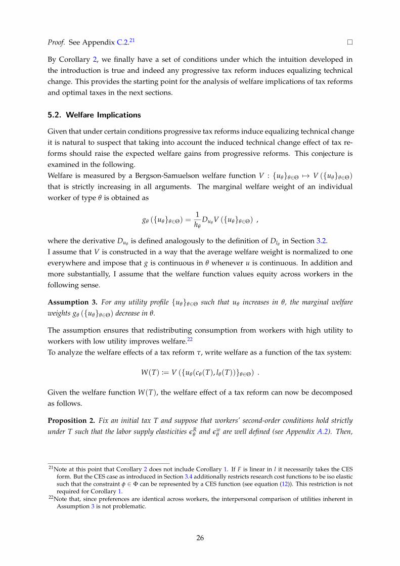
5.2. Welfare Implications

Given that under certain conditions progressive tax reforms induce equalizing technical changeit is natural to suspect that taking into account the induced technical change effect of tax re-forms should raise the expected welfare gains from progressive reforms. This conjecture isexamined in the following.Welfare is measured by a Bergson-Samuelson welfare function V : {uθ}θ∈Θ 7→ V ({uθ}θ∈Θ)

that is strictly increasing in all arguments. The marginal welfare weight of an individualworker of type θ is obtained as

gθ ({uθ}θ∈Θ) =1hθ

DuθV ({uθ}θ∈Θ) ,

where the derivative Duθis defined analogously to the definition of Dlθ in Section 3.2.

I assume that V is constructed in a way that the average welfare weight is normalized to oneeverywhere and impose that g is continuous in θ whenever u is continuous. In addition andmore substantially, I assume that the welfare function values equity across workers in thefollowing sense.

Assumption 3. For any utility profile {uθ}θ∈Θ such that uθ increases in θ, the marginal welfareweights gθ ({uθ}θ∈Θ) decrease in θ.

The assumption ensures that redistributing consumption from workers with high utility toworkers with low utility improves welfare.22

To analyze the welfare effects of a tax reform τ, write welfare as a function of the tax system:

W(T) := V ({uθ(cθ(T), lθ(T))}θ∈Θ) .

Given the welfare function W(T), the welfare effect of a tax reform can now be decomposedas follows.

Proposition 2. Fix an initial tax T and suppose that workers’ second-order conditions hold strictlyunder T such that the labor supply elasticities εR

θ and εwθ are well defined (see Appendix A.2). Then,

21Note at this point that Corollary 2 does not include Corollary 1. If F is linear in l it necessarily takes the CESform. But the CES case as introduced in Section 3.4 additionally restricts research cost functions to be iso elasticsuch that the constraint φ ∈ Φ can be represented by a CES function (see equation (12)). This restriction is notrequired for Corollary 1.

22Note that, since preferences are identical across workers, the interpersonal comparison of utilities inherent inAssumption 3 is not problematic.

26

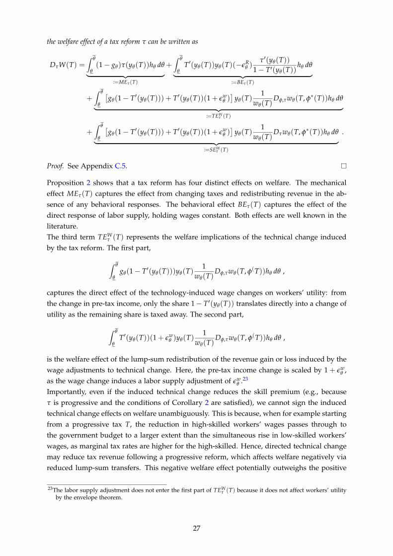
the welfare effect of a tax reform τ can be written as

DτW(T) =∫ θ

θ(1− gθ)τ(yθ(T))hθ dθ︸ ︷︷ ︸

:=MEτ(T)

+∫ θ

θT′(yθ(T))yθ(T)(−εR

θ )τ′(yθ(T))

1− T′(yθ(T))hθ dθ︸ ︷︷ ︸

:=BEτ(T)

+∫ θ

θ

[gθ(1− T′(yθ(T))) + T′(yθ(T))(1 + εw

θ )]

yθ(T)1

wθ(T)Dφ,τwθ(T, φ∗(T))hθ dθ︸ ︷︷ ︸

:=TEWτ (T)

+∫ θ

θ

[gθ(1− T′(yθ(T))) + T′(yθ(T))(1 + εw

θ )]

yθ(T)1

wθ(T)Dτwθ(T, φ∗(T))hθ dθ︸ ︷︷ ︸

:=SEWτ (T)

.

Proof. See Appendix C.5.

Proposition 2 shows that a tax reform has four distinct effects on welfare. The mechanicaleffect MEτ(T) captures the effect from changing taxes and redistributing revenue in the ab-sence of any behavioral responses. The behavioral effect BEτ(T) captures the effect of thedirect response of labor supply, holding wages constant. Both effects are well known in theliterature.The third term TEW

τ (T) represents the welfare implications of the technical change inducedby the tax reform. The first part,

∫ θ

θgθ(1− T′(yθ(T)))yθ(T)

1wθ(T)

Dφ,τwθ(T, φ(T))hθ dθ ,

captures the direct effect of the technology-induced wage changes on workers’ utility: fromthe change in pre-tax income, only the share 1− T′(yθ(T)) translates directly into a change ofutility as the remaining share is taxed away. The second part,

∫ θ

θT′(yθ(T))(1 + εw

θ )yθ(T)1

wθ(T)Dφ,τwθ(T, φ(T))hθ dθ ,

is the welfare effect of the lump-sum redistribution of the revenue gain or loss induced by thewage adjustments to technical change. Here, the pre-tax income change is scaled by 1 + εw

θ ,as the wage change induces a labor supply adjustment of εw

θ .23

Importantly, even if the induced technical change reduces the skill premium (e.g., becauseτ is progressive and the conditions of Corollary 2 are satisfied), we cannot sign the inducedtechnical change effects on welfare unambiguously. This is because, when for example startingfrom a progressive tax T, the reduction in high-skilled workers’ wages passes through tothe government budget to a larger extent than the simultaneous rise in low-skilled workers’wages, as marginal tax rates are higher for the high-skilled. Hence, directed technical changemay reduce tax revenue following a progressive reform, which affects welfare negatively viareduced lump-sum transfers. This negative welfare effect potentially outweighs the positive

23The labor supply adjustment does not enter the first part of TEWτ (T) because it does not affect workers’ utility

by the envelope theorem.

27

effect coming from the reduction in pre-tax wage inequality through the induced technicalchange.24

The final term in Proposition 2, SEWτ (T) captures the welfare effect of the within-technology

substitution effects on wages caused by the tax reform. Its structure is analogous to that ofTEW

τ (T). Given that even the induced technical change component TEWτ (T) has an ambigu-

ous effect on welfare, it is not surprising that also the substitution component SEWτ (T) can

generally not be signed.Importantly, however, Proposition 2 can be combined with equations (26) and (51) for therelative wage effects of tax reforms from Propositions 1 and 6 (in Appendix C.3). This yieldsa formula for the welfare effects of tax reforms in terms of empirically observable quantitiesand welfare weights. I use this combination of expressions to quantify the welfare effects oftax reforms and the contribution of directed technical change in Section 7.The implications of Proposition 2 may be somewhat unexpected in light of the previous sec-tion’s result. After all, if a progressive reform induces equalizing technical change and thewelfare function values equity, directed technical change effects should make progressive re-forms in some way more attractive. To see precisely in which way this is indeed true, we mustslightly adjust the question posed by Proposition 2.Concretely, instead of asking how directed technical change alters the welfare effects of a givenprogressive tax reform, we now study how accounting for directed technical change affectsthe set of initial taxes under which welfare can be improved by some progressive reform. Inparticular, let

T := {T | T is CRP, ∃τ progressive s.t. DτW(T) > 0}

denote the set of CRP tax schedules that can be improved in a welfare sense by a progressivetax reform. The restriction to CRP taxes is imposed to invoke Corollary 2. Specifically, com-bining the CRP restriction with iso-elastic disutility of labor and the CES production structurefrom Section 3.4 ensures, according to Corollary 2, that any progressive tax reform inducesequalizing technical change.As a benchmark for comparison that does not include directed technical change effects, let

Dexτ W(T) := DτW(T)|ρθ,θ=0 ∀ θ,θ (28)

denote the welfare effect of a reform τ when counterfactually setting all technical changeelasticities to zero (or, put differently, when holding technology fixed). Then, we can define

T ex := {T | T is CRP, ∃τ progressive s.t. Dexτ W(T) > 0}

as the set of CRP schedules that one would perceive to be improvable by progressive reformsif one were to ignore directed technical change.Comparing the two thus defined sets we find that accounting for directed technical changeexpands the set of tax schedules under which welfare can be improved by a progressivereform.

24This is similar to the observation by Sachs et al. (2019) that within-technology substitution effects may increasethe revenue gains from progressive tax reforms if the initial tax schedule is already progressive.

28

Proposition 3. Suppose F and Φ are CES as introduced in Section 3.4 and the disutility of labor isiso elastic. Then,

T ex ⊆ T ,

that is, the set of initial tax schedules that can be improved by a progressive reform becomes larger whenaccounting for directed technical change effects.

Proof. See Appendix C.5.

This result proposes a way in which directed technical change effects make progressive re-forms more attractive. Specifically, accounting for directed technical change increases thescope for welfare improvements by progressive tax reforms. It aligns neatly with Corollary 2,whereby progressive reforms induce equalizing technical change, and with the correspondingintuition developed in the introduction.The idea behind Proposition 3 relies on the mechanism design approach to income taxation.It goes as follows. Consider a progressive tax reform that a tax planner who neglects directedtechnical change effects (the exogenous technology planner, henceforth) expects to raise wel-fare. For any such reform, a planner who correctly anticipates directed technical changeeffects (the endogenous technology planner, henceforth) can find another progressive reformthat exactly replicates the labor allocation expected by the exogenous technology planner fol-lowing his reform. But since progressive tax reforms induce equalizing technical change, theendogenous technology planner anticipates a more equal wage distribution after her reformthan the exogenous technology planner expects to find after his reform. Via incentive com-patibility constraints, a more equal wage distribution allows to distribute consumption moreequally as well. Hence, while the two planners expect the same labor allocation to materi-alize, the endogenous technology planner anticipates a more equal consumption distributionthan the exogenous technology planner. Since this reasoning holds for any progressive re-form of the exogenous technology planner, the endogenous technology planner can find awelfare-improving progressive reform whenever the exogenous technology planner can findone. Hence, the endogenous technology planner perceives the scope for welfare improvementsthrough progressive tax reforms to be greater.

6. Optimal Taxes

The results from the tax reform analysis suggest that directed technical change effects shouldrender the optimal tax scheme more progressive. I examine this conjecture in the following.For the characterization of optimal tax rates it is convenient to denote the average welfareweight across all types above a given type θ as

gθ :=1

1− Hθ

∫ θ

θgθhθ dθ .

Moreover, for a function x : (θ, z) 7→ xθ(z) (e.g., wages or labor inputs) that depends on θ and

29

potentially further variables z, I denote the derivative of x with respect to θ by

x′θ(z) :=dxθ(z)

dθ

and the corresponding semi-elasticity by

xθ(z) :=x′θ(z)xθ(z)

.

Finally, without loss of generality let worker types be ordered according to their wages underthe optimum tax schedule, that is, under the optimal tax wθ ≤ wθ if θ ≤ θ.To derive optimal tax rates, I follow the mechanism design approach to optimal taxation as itprovides the fastest route ot the central results presented below.25 For that, write welfare as afunction of consumption and labor allocations instead of utility levels:

W(c, l) := V ({uθ(cθ , lθ)}θ∈Θ}) .

The goal is to find the consumption-labor allocation that maximizes welfare W(c, l) subjectto the aggregate resource constraint and to incentive compatibility constraints across workertypes. The optimal tax schedule is then obtained as the tax that implements the welfare-maximizing allocation.The aggregate resource constraint is given by

∫ θ

θcθhθ dθ = F(l, φ∗(l)) . (29)

Incentive compatibility requires

uθ = maxθ∈Θ

{cθ − v

(wθ lθ

wθ

)}∀ θ .

I restrict attention to instances of the model where the labor input under the optimal tax is C1

almost everywhere and continuous in θ. Moreover, I assume that this property of labor inputsextends to wages as follows.

Assumption 4. Aggregate production F satisfies the following. If l is C1 almost everywhere andcontinuous in θ, then Dlθ F(l, φ) is C1 almost everywhere and continuous in θ for all φ ∈ Φ.

Under this restriction and with the wage function wθ increasing in θ at the optimum, theincentive compatibility constraint is equivalent to the following conditions:

c′θ = v′(lθ)(w′θ lθ + wθ l′θ)1

wθfor almost every θ, (30)

y′θ ≥ 0 for almost every θ . (31)

25The alternative approach would be to use the formulas for the welfare effects of tax reforms from Section 5.2and impose that these effects are zero for all reforms at the optimum. The two approaches yield the sameresults.

30

As is usual in the literature, I drop the monotonicity requirement (31) and study the relaxedproblem of maximizing welfare subject to (29) and (30).26

From the incentive compatibility and resource constraints, consumption levels can be derivedas a function of labor inputs. I substitute this function into the welfare function W andtake first-order conditions with respect to labor inputs. Using workers’ first-order conditionto reintroduce marginal tax rates into the problem then yields the following expression foroptimal marginal tax rates.

Proposition 4. Suppose the labor input l under the optimal tax is C1 in θ almost everywhere. Then,at almost every type θ, optimal marginal tax rates satisfy the following conditions.

T′(yθ)

1− T′(yθ)= PE∗θ + TE∗θ + SE∗θ ,

where

PE∗θ =

(1 +

1eθ

)1− Nwθ

nwθwθ

(1− gθ)

TE∗θ = lim∆→0

1∆

∫ θ

θ

1− T′(yθ)

1− T′(yθ)

1− Hθ

hθwθ(1− gθ)yθ

dwθ(l, φ∗(l + µl∆,θ))

dµ

∣∣∣∣∣µ=0

dθ

SE∗θ = lim∆→0

1∆

∫ θ

θ

1− T′(yθ)

1− T′(yθ)

1− Hθ

hθwθ(1− gθ)yθ

dwθ(l + µl∆,θ , φ∗(l))dµ

∣∣∣∣∣µ=0

dθ ,

all variables are evaluated at equilibrium under the optimal tax T, and N and m denote the cumulativedistribution and the density function of wages at the optimum.Moreover, if l′θ exists on some left (right) neighborhood of θ (θ) and lim supθ→θ l′θ < ∞ (lim infθ→θ l′θ >−∞) under the optimal tax,27 then

TE∗θ ≤ 0 and TE∗θ≥ 0 .

Proof. See Appendix D.1.

Proposition 4 provides an expression that decomposes the optimal tax rates into three terms.The first term PE∗θ is the standard expression that would be obtained in a setting with exoge-nous wages. It is zero at the bottom and the top income level, reflecting the well-known resultthat the optimal marginal tax rate is zero for the highest and the lowest income earner whenwages are exogenous.The second term, TE∗θ , captures the impact of directed technical change effects on the optimaltax. It is negative at the bottom and positive at the top income. The intuition behind thesesigns is closely related to the intuition for the positive influence of directed technical changeeffects on the scope for welfare improvements through progressive tax reforms described in

26In all quantitative simulations of optimal taxes, I verify that the monotonicity condition (31) holds at the opti-mum.

27This assumption guarantees that the distribution of labor inputs is well behaved at the top and at the bottom,in the sense that its density is continuous and strictly positive on some neighborhood of the top or the bottomtype, respectively. This in turn allows to evaluate the effects of the labor input perturbations l∆,θ and l∆,θ onrelative labor inputs and invoke the directed technical change results of Section 4.

31

Section 5.2. By reducing marginal tax rates at the bottom and increasing them at the top, theoptimal tax schedule stimulates the relative labor supply of less skilled workers, thus inducingfirms to operate technologies with a higher relative productivity for low-skilled workers. Thisraises low-skilled workers’ wages relative to those of high-skilled workers. In the mechanismdesign problem, the ensuing compression in the pre-tax wage distribution slackens high-skilled workers’ incentive compatibility constraints and widens the scope for redistribution.The third term, SE∗θ , comes from within-technology substitution effects. Without further re-striction, there is too little structure imposed on the aggregate production function F to signthe impact of within-technology substitution effects on optimal marginal tax rates at any pointof the income distribution.For the CES case, Lemma 9 in Appendix D.2 provides specific versions of the terms SE∗θand TE∗θ . There, TE∗θ is strictly positive at the top and strictly negative at the bottom. Thesubstitution term has the opposite signs. It is strictly negative at the top and strictly positiveat the bottom. This recovers the results from Stiglitz (1987), who shows, in a model with onlytwo types of workers, that within-technology substitution effects raise optimal marginal taxrates at the bottom and lower them at the top.Appendix D.2 also shows that the combined impact of directed technical change and within-technology substitution effects depends on condition (19) for strong bias. If there is strongbias, the technical change term TE∗θ dominates the substitution term SE∗θ , leading to a positivemarginal tax rate at the top and a negative marginal tax at the bottom. Inversely, if there isno strong bias, the optimal marginal tax rate is positive at the bottom and negative at the top,following the logic of Stiglitz (1987).It is well known in the literature that results for optimal marginal tax rates at the highestincome level are very local. They do not extend approximately to incomes even slightly belowthe top. To derive analytical insights into the structure of optimal tax rates over more relevantranges of the income distribution, it is useful to consider the CES case in more detail.Using the CES versions of TE∗θ and SE∗θ from Appendix D.2, the conditions for optimalmarginal tax rates simplify as follows.

Proposition 5. Suppose the conditions of Proposition 4 are satisfied and F and Φ take the CES formintroduced in Section 3.4. Then, at almost every type θ, optimal marginal tax rates satisfy the followingconditions.

T′(yθ)

1− T′(yθ)=

(1 +

1eθ

)1− Bβθ

bβθβθ

(1− gθ) + γCES(1− gθ) + ρCES(1− gθ) , (32)

where all variables are evaluated at equilibrium under the optimal tax T, the function β : θ 7→ βθ isgiven by

βθ := κ1+γCES+ρCES

θ hγCES+ρCES

θ ∀ θ ,

while B and b are the cumulative distribution and the density function of β.

Proof. See Appendix D.2.

Proposition 5 provides a Diamond (1998) style expression for optimal marginal tax rates,

32

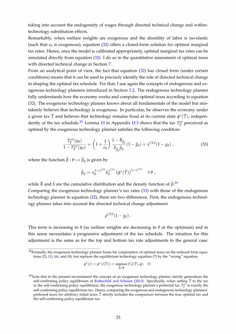
taking into account the endogeneity of wages through directed technical change and within-technology substitution effects.Remarkably, when welfare weights are exogenous and the disutility of labor is iso-elastic(such that eθ is exogenous), equation (32) offers a closed-form solution for optimal marginaltax rates. Hence, once the model is calibrated appropriately, optimal marginal tax rates can besimulated directly from equation (32). I do so in the quantitative assessment of optimal taxeswith directed technical change in Section 7.From an analytical point of view, the fact that equation (32) has closed form (under certainconditions) means that it can be used to precisely identify the role of directed technical changein shaping the optimal tax schedule. For that, I use again the concepts of endogenous and ex-ogenous technology planners introduced in Section 5.2. The endogenous technology plannerfully understands how the economy works and computes optimal taxes according to equation(32). The exogenous technology planner knows about all fundamentals of the model but mis-takenly believes that technology is exogenous. In particular, he observes the economy undera given tax T and believes that technology remains fixed at its current state φ∗(T), indepen-dently of the tax schedule.28 Lemma 10 in Appendix D.3 shows that the tax Tex

Tperceived as

optimal by the exogenous technology planner satisfies the following condition:

Tex′T

(yθ)

1− Tex′T

(yθ)=

(1 +

1eθ

) 1− Bβθ

bβθβθ

(1− gθ) + γCES(1− gθ) , (33)

where the function β : θ 7→ βθ is given by

βθ := κ1+γCES

θ hγCES

θ

(φ∗(T)

)1+γCES

∀ θ ,

while B and b are the cumulative distribution and the density function of β.29

Comparing the exogenous technology planner’s tax rates (33) with those of the endogenoustechnology planner in equation (32), there are two differences. First, the endogenous technol-ogy planner takes into account the directed technical change adjustment

ρCES(1− gθ) .

This term is increasing in θ (as welfare weights are decreasing in θ at the optimum) and inthis sense necessitates a progressive adjustment of the tax schedule. The intuition for thisadjustment is the same as for the top and bottom tax rate adjustments in the general case:

28Formally, the exogenous technology planner bases his computation of optimal taxes on the reduced form equa-tions (2), (1), (6), and (8), but replaces the equilibrium technology equation (7) by the “wrong” equation

φ∗(l) = φ∗(l(T)) = argmaxφ∈Φ

F(l(T), φ) ∀l .

29Note that in the present environment the concept of an exogenous technology planner strictly generalizes theself-confirming policy equilibrium of Rothschild and Scheuer (2013). Specifically, when setting T to the taxin the self-confirming policy equilibrium, the exogenous technology planner’s preferred tax Tex

Tis exactly the

self-confirming policy equilibrium tax. Hence, comparing the exogenous and endogenous technology planners’preferred taxes for arbitrary initial taxes T strictly includes the comparison between the true optimal tax andthe self-confirming policy equilibrium tax.

33

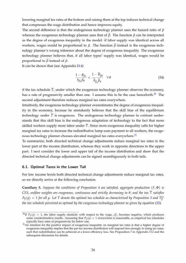
lowering marginal tax rates at the bottom and raising them at the top induces technical changethat compresses the wage distribution and hence improves equity.The second difference is that the endogenous technology planner uses the hazard ratio of β

whereas the exogenous technology planner uses that of β. The function β can be interpretedas the degree of exogenous inequality in the model: if labor supply was identical across allworkers, wages would be proportional to β. The function β instead is the exogenous tech-nology planner’s wrong inference about the degree of exogenous inequality. The exogenoustechnology planner believes that, if all labor types’ supply was identical, wages would beproportional to β instead of β.It can be shown that (see Appendix D.4)

1− Bβθ

bβθβθ

<1− Bβθ

bβθβθ

∀ θ (34)

if the tax schedule T, under which the exogenous technology planner observes the economy,has a rate of progressivity smaller than one. I assume this to be the case henceforth.30 Thesecond adjustment therefore reduces marginal tax rates everywhere.Intuitively, the exogenous technology planner overestimates the degree of exogenous inequal-ity in the economy, because he mistakenly believes that the skill bias of the equilibriumtechnology under T is exogenous. The endogenous technology planner in contrast under-stands that this skill bias is the endogenous adaptation of technology to the fact that moreskilled workers supply more labor under T. Since more exogenous inequality calls for highermarginal tax rates to increase the redistributive lump-sum payment to all workers, the exoge-nous technology planner chooses elevated marginal tax rates everywhere.31

To summarize, both directed technical change adjustments reduce marginal tax rates in thelower part of the income distribution, whereas they work in opposite directions in the upperpart. I next consider the lower and upper tail of the income distribution and show that thedirected technical change adjustments can be signed unambiguously in both tails.

6.1. Optimal Taxes in the Lower Tail

For low income levels both directed technical change adjustments reduce marginal tax rates,so we directly arrive at the following conclusion.

Corollary 3. Suppose the conditions of Proposition 4 are satisfied, aggregate production (F, Φ) isCES, welfare weights are exogenous, continuous and strictly decreasing in θ, and the tax T satisfiesPT(y) < 1 for all y. Let T denote the optimal tax schedule as characterized by Proposition 5 and Tex

Tthe tax schedule perceived as optimal by the exogenous technology planner as given by equation (33).

30If PT(y) > 1, the labor supply elasticity with respect to the wage, εwθ , becomes negative, which produces

some counterintuitive results. Assuming that PT(y) < 1 everywhere is reasonable, as empirical tax schedulestypically have rates of progressivity far below one.

31An intuition for the positive impact of exogenous inequality on marginal tax rates is that a higher degree ofexogenous inequality implies that the pre-tax income distribution will respond less strongly to rising tax rates,such that redistribution can be achieved at a lower efficiency loss. See Proposition 7 in Appendix D.2 and thesubsequent discussion for details.

34

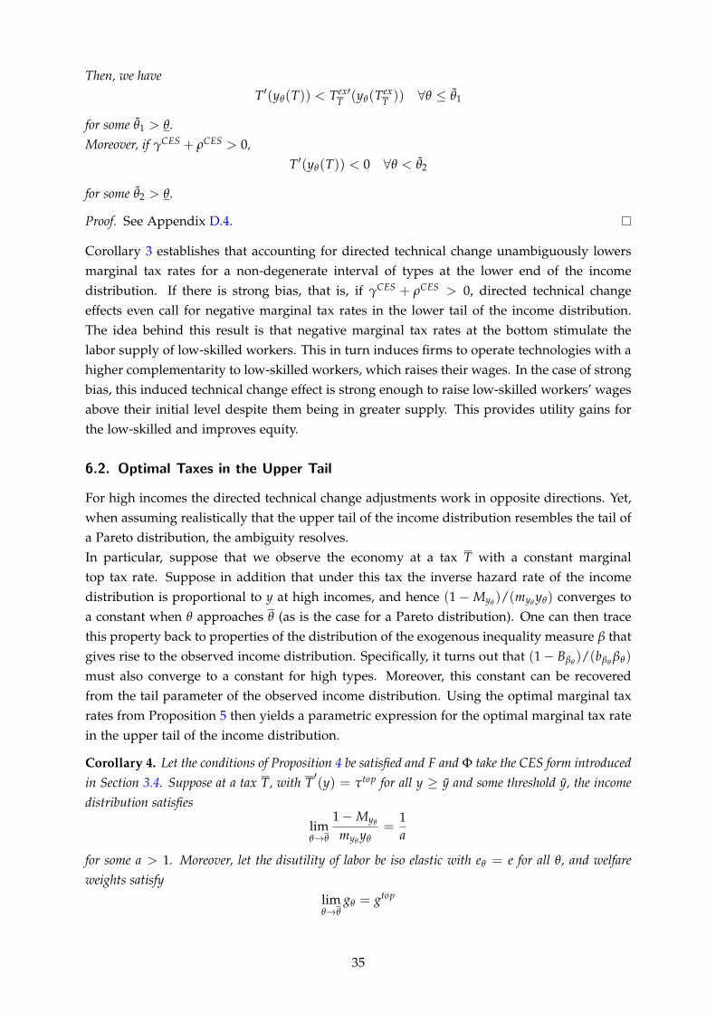
Then, we haveT′(yθ(T)) < Tex′

T (yθ(TexT )) ∀θ ≤ θ1

for some θ1 > θ.Moreover, if γCES + ρCES > 0,

T′(yθ(T)) < 0 ∀θ < θ2

for some θ2 > θ.

Proof. See Appendix D.4.

Corollary 3 establishes that accounting for directed technical change unambiguously lowersmarginal tax rates for a non-degenerate interval of types at the lower end of the incomedistribution. If there is strong bias, that is, if γCES + ρCES > 0, directed technical changeeffects even call for negative marginal tax rates in the lower tail of the income distribution.The idea behind this result is that negative marginal tax rates at the bottom stimulate thelabor supply of low-skilled workers. This in turn induces firms to operate technologies with ahigher complementarity to low-skilled workers, which raises their wages. In the case of strongbias, this induced technical change effect is strong enough to raise low-skilled workers’ wagesabove their initial level despite them being in greater supply. This provides utility gains forthe low-skilled and improves equity.

6.2. Optimal Taxes in the Upper Tail

For high incomes the directed technical change adjustments work in opposite directions. Yet,when assuming realistically that the upper tail of the income distribution resembles the tail ofa Pareto distribution, the ambiguity resolves.In particular, suppose that we observe the economy at a tax T with a constant marginaltop tax rate. Suppose in addition that under this tax the inverse hazard rate of the incomedistribution is proportional to y at high incomes, and hence (1−Myθ

)/(myθyθ) converges to

a constant when θ approaches θ (as is the case for a Pareto distribution). One can then tracethis property back to properties of the distribution of the exogenous inequality measure β thatgives rise to the observed income distribution. Specifically, it turns out that (1− Bβθ

)/(bβθβθ)

must also converge to a constant for high types. Moreover, this constant can be recoveredfrom the tail parameter of the observed income distribution. Using the optimal marginal taxrates from Proposition 5 then yields a parametric expression for the optimal marginal tax ratein the upper tail of the income distribution.

Corollary 4. Let the conditions of Proposition 4 be satisfied and F and Φ take the CES form introducedin Section 3.4. Suppose at a tax T, with T′(y) = τtop for all y ≥ y and some threshold y, the incomedistribution satisfies

limθ→θ

1−Myθ

myθyθ

=1a

for some a > 1. Moreover, let the disutility of labor be iso elastic with eθ = e for all θ, and welfareweights satisfy

limθ→θ

gθ = gtop

35

at the optimal tax.Then, the optimal tax T satisfies

limθ→θ

T′(yθ)

1− T′(yθ)=

1− gtop

ae+

a− 1a

γCES(1− gtop) +a− 1

aρCES(1− gtop) . (35)

Proof. See Appendix D.4.

Complementing Corollary 4, Corollary 6 in Appendix D.4 shows that under the same condi-tions the exogenous technology planner’s preferred tax satisfies

limθ→θ

Tex′T

(yθ)

1− Tex′T

(yθ)=

1− gtop

ae+

a− 1a

γCES(1− gtop) .

This expression is smaller than the endogenous technology planner’s preferred rate (35).Hence, taking into account directed technical change when designing optimal taxes leads tounambiguously higher marginal tax rates in the upper (Pareto) tail of the income distribution.

7. Quantitative Analysis

To assess the quantitative relevance of directed technical change effects, I calibrate the CESversion of the model to estimates from the empirical literature on directed technical change. Iuse the calibration to simulate the effects of tax reforms and to compute optimal taxes for theendogenous and the exogenous technology planner.

7.1. Calibration

The calibration proceeds as follows. First, I set the wage elasticity parameters γCES and ρCES

(equivalently, σ and δ), the labor supply elasticity e (assuming iso-elastic disutility of labor),and the initial tax function T (approximating the US income tax system in 2005) on the basis ofexisting empirical estimates. In the second step, I infer the exogenous technology parameterκ from the US income distribution in 2005.

Within-Technology Substitution Effects The within-technology substitution elasticity γCES

and the induced technical change elasticity ρCES govern the response of relative wages tochanges in relative labor inputs. Induced technical change effects are likely to arise withconsiderable delay, implying that to measure ρCES, one has to track relative wages over along period of time after an exogenous change in labor inputs occurred. Within-technologysubstitution, in contrast, does not require firms to change their production technology, soits effects are likely to occur over a much shorter period of time. The timing of the effectstherefore provides an opportunity to identify γCES and ρCES separately.The empirical literature that aims to identify an elasticity of substitution between differentiallyskilled worker groups without explicit reference to directed technical change has typicallyfocused on comparably short time periods of about one year or slightly more. I take theseestimates to set γCES.

36

Besides the timing of the effects, an important property in which many empirical studiesdiffer is the definition of the skill groups between which an elasticity of substitution is es-timated. Many studies focus on college graduates versus those without a college degree.Others, however, consider high school graduates versus high school dropouts. Dustmann,Frattini and Preston (2013) stand out in that they estimate substitution elasticities betweenworkers located at 20 different points in the wage distribution. They test for heterogeneity inthese elasticities but find no evidence for it. In light of this result, the CES assumption, whichimposes a single elasticity of substitution between any two disjoint groups of workers, seemsan acceptable simplification. It implies that all estimates, irrespective of the definition of skillgroups, are equally relevant for the calibration of γCES.Acemoglu (2002) summarizes the consensus of the literature at that time as σ being somewherebetween 1.4 and 2, which implies that γCES falls between −0.5 and −0.7. The results ofCarneiro et al. (2019) imply a short-run elasticity, measured within two years after the skillsupply shock, of −0.5 (for a detailed description of Carneiro et al. 2019 see below). This valuefalls within the consensus range observed by Acemoglu (2002). Moreover, Carneiro et al.(2019) is the only study that estimates wage responses at different points in time. Thereby,it provides estimates of γCES and ρCES obtained consistently within a single framework. Forthese reasons I set γCES = −0.5, the estimate implied by Carneiro et al. (2019).

Directed Technical Change Effects A few studies measure the response of wages to skillsupply shocks over substantially longer periods of time (about 10 years or more). Most ofthem explicitly reference directed technical change and provide evidence for technology ad-justments being an important driver of the long-run wage responses. Since this applies onlyto a handful of papers, I give a brief overview over each of them in Appendix E.1.Table 1 shows the results of these papers. The short-run estimates are −0.55 and −0.53,which (further) motivates my choice of γCES. Estimates over a period of about 10 years areconsistently close to zero, ranging from −0.1 to 0. Finally, the estimate from Carneiro et al.(2019) for an adjustment period of 17 years shows an effect of 0.5. These long-run effects aretotal effects, in the sense that they include both within-technology and between-technology(directed technical change) substitution. Hence, they map into the sum of γCES and ρCES.Based on Table 1 I will consider two cases. The first case, derived from the 10 year estimates,sets γCES + ρCES to −0.1, which, given the set value for γCES, implies ρCES = 0.4. In this case,within-technology substitution and directed technical change effects are of similar magnitudesand almost cancel each other (given that they work in opposite directions). Hence, accountingfor directed technical change puts the analysis back close to the case with exogenous wagesstudied extensively in the literature on optimal taxation. In the second case, based on the 17year estimate of Carneiro et al. (2019), I set γCES + ρCES to 0.5, such that ρCES = 1. In this case,directed technical change dominates within-technology substitution, that is, there is strongbias (see Section 4). I therefore call this the strong bias case.The conservative case is supported by all four studies in Table 1. Moreover, there are at leasttwo further papers that, for different reasons, do not provide estimates that could be usedto infer γCES and ρCES, but nevertheless support the view of the conservative case that the

37

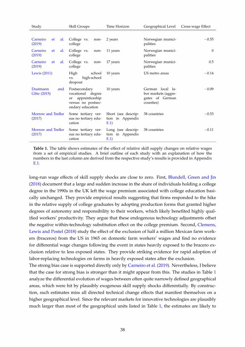
Study Skill Groups Time Horizon Geographical Level Cross-wage Effect

Carneiro et al.(2019)

College vs. non-college

2 years Norwegian munici-palities

−0.55

Carneiro et al.(2019)

College vs. non-college

11 years Norwegian munici-palities

0

Carneiro et al.(2019)

College vs. non-college

17 years Norwegian munici-palities

0.5

Lewis (2011) High schoolvs. high-schooldropout

10 years US metro areas −0.14

Dustmann andGlitz (2015)

Postsecondaryvocational degreeor apprenticeshipversus no postsec-ondary education

10 years German local la-bor markets (aggre-gates of Germancounties)

−0.09

Morrow and Trefler(2017)

Some tertiary ver-sus no tertiary edu-cation

Short (see descrip-tion in AppendixE.1)

38 countries −0.53

Morrow and Trefler(2017)

Some tertiary ver-sus no tertiary edu-cation

Long (see descrip-tion in AppendixE.1)

38 countries −0.11

Table 1. The table shows estimates of the effect of relative skill supply changes on relative wagesfrom a set of empirical studies. A brief outline of each study with an explanation of how thenumbers in the last column are derived from the respective study’s results is provided in AppendixE.1.

long-run wage effects of skill supply shocks are close to zero. First, Blundell, Green and Jin(2018) document that a large and sudden increase in the share of individuals holding a collegedegree in the 1990s in the UK left the wage premium associated with college education basi-cally unchanged. They provide empirical results suggesting that firms responded to the hikein the relative supply of college graduates by adopting production forms that granted higherdegrees of autonomy and responsibility to their workers, which likely benefited highly qual-ified workers’ productivity. They argue that these endogenous technology adjustments offsetthe negative within-technology substitution effect on the college premium. Second, Clemens,Lewis and Postel (2018) study the effect of the exclusion of half a million Mexican farm work-ers (braceros) from the US in 1965 on domestic farm workers’ wages and find no evidencefor differential wage changes following the event in states heavily exposed to the bracero ex-clusion relative to less exposed states. They provide striking evidence for rapid adoption oflabor-replacing technologies on farms in heavily exposed states after the exclusion.The strong bias case is supported directly only by Carneiro et al. (2019). Nevertheless, I believethat the case for strong bias is stronger than it might appear from this. The studies in Table 1analyze the differential evolution of wages between often quite narrowly defined geographicalareas, which were hit by plausibly exogenous skill supply shocks differentially. By construc-tion, such estimates miss all directed technical change effects that manifest themselves on ahigher geographical level. Since the relevant markets for innovative technologies are plausiblymuch larger than most of the geographical units listed in Table 1, the estimates are likely to

38

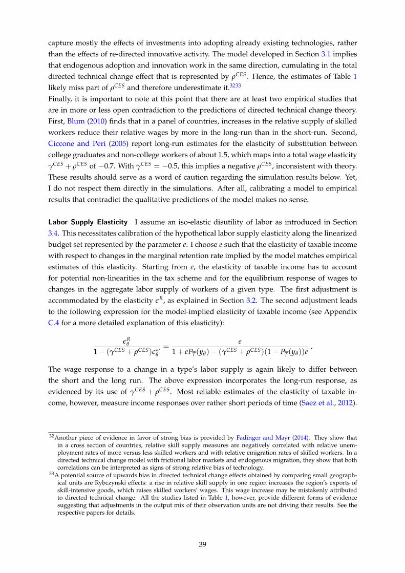
capture mostly the effects of investments into adopting already existing technologies, ratherthan the effects of re-directed innovative activity. The model developed in Section 3.1 impliesthat endogenous adoption and innovation work in the same direction, cumulating in the totaldirected technical change effect that is represented by ρCES. Hence, the estimates of Table 1likely miss part of ρCES and therefore underestimate it.3233

Finally, it is important to note at this point that there are at least two empirical studies thatare in more or less open contradiction to the predictions of directed technical change theory.First, Blum (2010) finds that in a panel of countries, increases in the relative supply of skilledworkers reduce their relative wages by more in the long-run than in the short-run. Second,Ciccone and Peri (2005) report long-run estimates for the elasticity of substitution betweencollege graduates and non-college workers of about 1.5, which maps into a total wage elasticityγCES + ρCES of −0.7. With γCES = −0.5, this implies a negative ρCES, inconsistent with theory.These results should serve as a word of caution regarding the simulation results below. Yet,I do not respect them directly in the simulations. After all, calibrating a model to empiricalresults that contradict the qualitative predictions of the model makes no sense.

Labor Supply Elasticity I assume an iso-elastic disutility of labor as introduced in Section3.4. This necessitates calibration of the hypothetical labor supply elasticity along the linearizedbudget set represented by the parameter e. I choose e such that the elasticity of taxable incomewith respect to changes in the marginal retention rate implied by the model matches empiricalestimates of this elasticity. Starting from e, the elasticity of taxable income has to accountfor potential non-linearities in the tax scheme and for the equilibrium response of wages tochanges in the aggregate labor supply of workers of a given type. The first adjustment isaccommodated by the elasticity εR, as explained in Section 3.2. The second adjustment leadsto the following expression for the model-implied elasticity of taxable income (see AppendixC.4 for a more detailed explanation of this elasticity):

εRθ

1− (γCES + ρCES)εwθ

=e

1 + ePT(yθ)− (γCES + ρCES)(1− PT(yθ))e.

The wage response to a change in a type’s labor supply is again likely to differ betweenthe short and the long run. The above expression incorporates the long-run response, asevidenced by its use of γCES + ρCES. Most reliable estimates of the elasticity of taxable in-come, however, measure income responses over rather short periods of time (Saez et al., 2012).

32Another piece of evidence in favor of strong bias is provided by Fadinger and Mayr (2014). They show thatin a cross section of countries, relative skill supply measures are negatively correlated with relative unem-ployment rates of more versus less skilled workers and with relative emigration rates of skilled workers. In adirected technical change model with frictional labor markets and endogenous migration, they show that bothcorrelations can be interpreted as signs of strong relative bias of technology.

33A potential source of upwards bias in directed technical change effects obtained by comparing small geograph-ical units are Rybczynski effects: a rise in relative skill supply in one region increases the region’s exports ofskill-intensive goods, which raises skilled workers’ wages. This wage increase may be mistakenly attributedto directed technical change. All the studies listed in Table 1, however, provide different forms of evidencesuggesting that adjustments in the output mix of their observation units are not driving their results. See therespective papers for details.

39

Hence, a more appropriate theoretical counterpart of these estimates is given by the expression

εRθ :=

e1 + ePT(yθ)− γCES(1− PT(yθ))e

,

which only includes the wage effects of within-technology factor substitution. I use this ex-pression to calibrate e given estimates of εR

θ . In doing so, I set PT to 0, as empirical tax systemsare piece-wise linear.Following Saez et al. (2012), who partially review the extensive literature on the elasticity oftaxable income, I choose a value of 0.25 for εR

θ . This maps into a value for e of 0.27. In thesimulations of tax reforms effects on wages, I will also experiment with a larger labor supplyelasticity located more towards the upper bound of empirical estimates. For that, I use thetaxable income elasticity of 0.57 from Gruber and Saez (2002), which Diamond and Saez (2011)call a conservative upper bound. The implied value for e is 0.64.

Initial Tax System I set the initial tax system, denoted by T, as an approximation to theUS income tax in 2005. I follow Heathcote et al. (2017), who show that a constant-rate-of-progressivity schedule as introduced in Section 3.4 provides a good approximation. Heathcoteet al. (2017) estimate the parameters of such a tax function on 2000 to 2005 income and tax datafor the US and obtain values of p = 0.181 and λ = 5.568. I use these values in all simulations.

Exogenous Technology With the parameters γCES, ρCES, e, and T calibrated, the exogenoustechnology parameter κ is identified by the income distribution under the initial tax systemT. I approximate the income distribution by smoothly combining a lognormal distribution forincomes below $200k and a Pareto distribution with tail parameter 1.5 above $200k (Diamondand Saez, 2011). Moreover, I assume that the type distribution h is standard uniform on [θ, θ] =

[0, 1]. In the CES case, this assumption is insubstantial, because the cross-wage elasticitybetween any two distinct types of workers is independent of the types’ locations in the typespace. Given an estimate of the income distribution, it is straightforward to compute thefunction κ from workers’ first-order condition (2) and the wage equation (13). The procedureis described in more detail in Appendix E.2.

Welfare Function Finally, I use a welfare function of the type

V({uθ}θ∈Θ) =∫ θ

θ

11− r

u1−rθ hθ dθ ,

where the relative inequality aversion parameter r allows to vary the strength of the preferencefor equity inherent in the welfare function in a flexible way (Atkinson, 1970).

7.2. Simulation

Given the calibrated CES version of the model, I simulate the effect of tax reforms on wagesand welfare and compute optimal taxes on the basis of the analytical results of Sections 5 and6.

40

0 0.2 0.4 0.6 0.8 1-10

-5

0

5

10

Type Measured by Percentile of the Wage Distribution

Wag

eC

hang

ein

%

Standard Labor Supply Elasticity, e = 0.27

ρ = 1 and γ = -0.5ρ = 0.4 and γ = -0.5Exo. Tech. Planner (γ = -0.5)

0 0.2 0.4 0.6 0.8 1-10

-5

0

5

10

Type Measured by Percentile of the Wage Distribution

Wag

eC

hang

ein

%

High Labor Supply Elasticity, e = 0.64

ρ = 1 and γ = -0.5ρ = 0.4 and γ = -0.5Exo. Tech. Planner (γ = -0.5)

Figure 1. The figure displays the total wage changes in log points induced by the progressive taxreform described in the text. In the left panel, the labor supply elasticity takes its standard valueof e = 0.27. The right panel shows wage changes for a high value of e = 0.64. Wage changes aregiven for workers at each percentile in the (pre- and post-reform) wage distribution. In each panel,the three plots show the wage changes predicted in the strong bias case (ρ = 1), in the conservativecase (ρ = 0.4), and by the exogenous technology planner (ρ = 0).

Tax Reforms To assess the results on the effects of tax reforms quantitatively, I study ahypothetical tax reform that reverses the cumulative impact on tax progressivity of US incometax reforms from 1970 to 2005. As documented by Piketty and Saez (2007), the US income taxsystem underwent a series of regressive reforms in this period. Heathcote et al. (2017) estimatethe decline in tax progressivity between 1970 and 2005 to be 0.034 when measured by theprogressivity parameter of a constant-rate-of-progressivity tax schedule. Taking as a startingvalue the progressivity estimate of p = 0.181, I hence ask what are the effects of raising theprogressivity of a constant-rate-of-progressivity tax from 0.181 (its 2005 US value) to 0.215 (its1970 US value).34

In the case of strong bias (ρCES + γCES > 0), such a progressive reform will reduce wage in-equality. A particular focus of the analysis will thus be whether taking back the regressivetax reforms of the past decades would result in a meaningful reduction in US wage inequalitywhen accepting the strong bias calibration described above. Reversedly, the results are infor-mative about whether regressive tax reforms could have played a role, via directed technicalchange effects, in the rise of US wage inequality observed over the period under consideration.I compute the wage effects of the described reform using the expressions provided by Corol-laries 2 and 5. For the exogenous technology planner, who ignores directed technical change,the effects are given by equation (53) in Corollary 5. For the two cases with directed technicalchange effects, total wage effects are given by the sum of (the right-hand-sides of) equations(27) and (53).The results are displayed in the left panel of Figure 1. In the conservative case, the reformhas almost no effect on wages. This was expected, because directed technical change and

34I choose the post-reform value for the parameter λ (the second parameter of a constant-rate-of-progressivitytax function) such that, in the conservative case described above (ρCES = 0.4), the reform leaves tax revenueunchanged.

41

within-technology substitution effects cancel each other approximately in this case. The ex-ogenous technology planner predicts moderate wage decreases for low-skilled workers andeven smaller gains for the high-skilled. Even in the strong bias case, wage effects are modest.Wages for low-skilled workers rise by less than 2% while wages for high-skilled workers fallby less than 1%. Towards the very ends of the wage distribution, the effects become somewhatstronger, but only few workers are affected by these more substantial changes.To put the results into perspective, I compute the predicted change in the ratio between the90th and the 10th percentile of the wage distribution. In the conservative case, this amounts to−0.2%, whereas in the strong bias case the ratio changes by about−1% percent. These changescan be compared to the actually observed changes in the US wage distribution between 1970and 2005. The data presented in Acemoglu and Autor (2011) suggest that the 90-10-percentileratio of wages rose by about 30% percent between 1970 and 2005. Compared to this increasein inequality, the effects of the tax reforms that took place between 1970 and 2005 on the USwage distribution seem rather small even in the strong bias case.A likely explanation for this somewhat sobering result is that the labor supply responses to taxreforms found in the empirical literature, reflected in the elasticity parameter e, are typicallysmall. Since the entire directed technical change effect of tax reforms is transmitted via laborsupply responses, the directed technical change effects tend to be small as well.To assess how sensitive the results are to the choice of the labor supply elasticity, the rightpanel of Figure 1 plots wage changes when e is set to 0.64. As argued in the previous section,this value falls into the high range of estimates from the empirical literature on taxable incomeelasticities. Expectedly, the results do not change remarkably for the conservative case. Forthe strong bias case, the predicted wage growth for low-wage earners approximately doublesfrom below 2 to almost 4%. Again computing the effect on the 90-10-percentile ratio yields avalue of −2.7%. Still, this is orders of magnitude below the total changes observed in the USwage distribution over the past 50 years.Finally, Figure 2 computes the percentage change in welfare induced by the tax reform fordifferent values of the relative inequality aversion parameter r (based on Proposition 2). Asobserved analytically, the influence of directed technical change effects on the welfare assess-ment of a given progressive reform is ambiguous. The figure shows that for lower degreesof inequality aversion, directed technical change raises the welfare gains from the progres-sive reform. Here, the reduction in wage inequality induced by directed technical changeoutweighs the loss in tax revenue, which translates into a reduction in the lump-sum pay-ment to all workers. For high values of inequality aversion, for which the welfare functionapproaches a Rawlsian objective, the negative revenue effect from directed technical changebecomes dominant, reducing the welfare gains from the reform. Interestingly, for very highlevels of inequality aversion, accounting for directed technical change even switches the signof the welfare effect. When ignoring directed technical change, the reform appears to raisewelfare; taking into account directed technical change effects makes the reform undesirable.Notwithstanding these results, Proposition 3 implies that even for such very high values ofinequality aversion, there must be a different progressive reform that raises welfare whenaccounting for directed technical change.

42

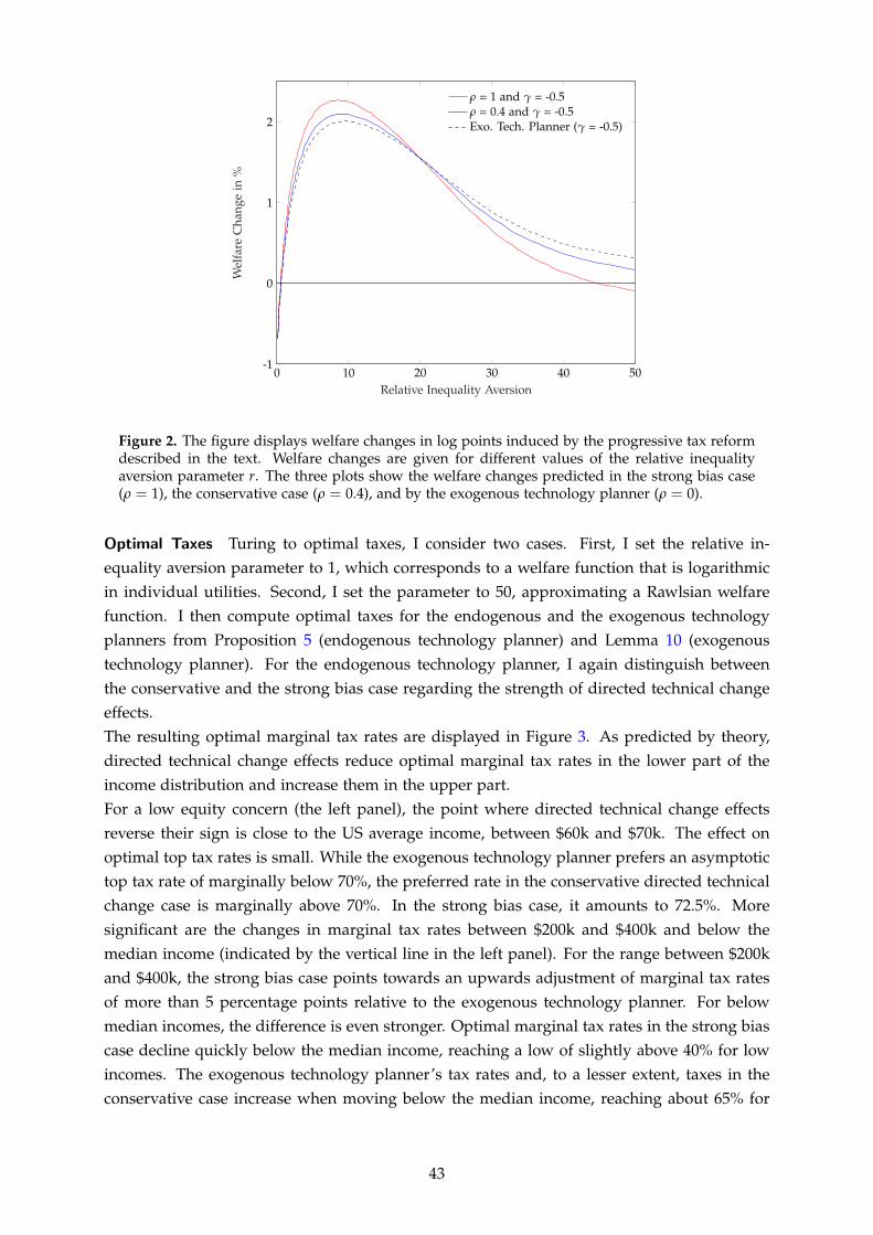
0 10 20 30 40 50-1

0

1

2

Relative Inequality Aversion

Wel

fare

Cha

nge

in%

ρ = 1 and γ = -0.5ρ = 0.4 and γ = -0.5Exo. Tech. Planner (γ = -0.5)

Figure 2. The figure displays welfare changes in log points induced by the progressive tax reformdescribed in the text. Welfare changes are given for different values of the relative inequalityaversion parameter r. The three plots show the welfare changes predicted in the strong bias case(ρ = 1), the conservative case (ρ = 0.4), and by the exogenous technology planner (ρ = 0).

Optimal Taxes Turing to optimal taxes, I consider two cases. First, I set the relative in-equality aversion parameter to 1, which corresponds to a welfare function that is logarithmicin individual utilities. Second, I set the parameter to 50, approximating a Rawlsian welfarefunction. I then compute optimal taxes for the endogenous and the exogenous technologyplanners from Proposition 5 (endogenous technology planner) and Lemma 10 (exogenoustechnology planner). For the endogenous technology planner, I again distinguish betweenthe conservative and the strong bias case regarding the strength of directed technical changeeffects.The resulting optimal marginal tax rates are displayed in Figure 3. As predicted by theory,directed technical change effects reduce optimal marginal tax rates in the lower part of theincome distribution and increase them in the upper part.For a low equity concern (the left panel), the point where directed technical change effectsreverse their sign is close to the US average income, between $60k and $70k. The effect onoptimal top tax rates is small. While the exogenous technology planner prefers an asymptotictop tax rate of marginally below 70%, the preferred rate in the conservative directed technicalchange case is marginally above 70%. In the strong bias case, it amounts to 72.5%. Moresignificant are the changes in marginal tax rates between $200k and $400k and below themedian income (indicated by the vertical line in the left panel). For the range between $200kand $400k, the strong bias case points towards an upwards adjustment of marginal tax ratesof more than 5 percentage points relative to the exogenous technology planner. For belowmedian incomes, the difference is even stronger. Optimal marginal tax rates in the strong biascase decline quickly below the median income, reaching a low of slightly above 40% for lowincomes. The exogenous technology planner’s tax rates and, to a lesser extent, taxes in theconservative case increase when moving below the median income, reaching about 65% for

43

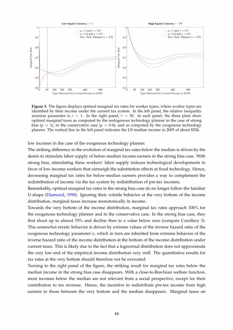
0 50 100 200 300 400 5000.4

0.5

0.6

0.7

0.8

0.9

1

Type Measured by Current Income in $1000

Mar

gina

lTax

Rat

e

Low Equity Concern, r = 1

ρ = 1 and γ = -0.5ρ = 0.4 and γ = -0.5Exo. Tech. Planner (γ = -0.5)

0 50 100 200 300 400 5000.4

0.5

0.6

0.7

0.8

0.9

1

Type Measured by Current Income in $1000

Mar

gina

lTax

Rat

e

High Equity Concern, r = 50

ρ = 1 and γ = -0.5ρ = 0.4 and γ = -0.5Exo. Tech. Planner (γ = -0.5)

Figure 3. The figure displays optimal marginal tax rates for worker types, where worker types areidentified by their income under the current tax system. In the left panel, the relative inequalityaversion parameter is r = 1. In the right panel, r = 50. In each panel, the three plots showoptimal marginal taxes as computed by the endogenous technology planner in the case of strongbias (ρ = 1), in the conservative case (ρ = 0.4), and as computed by the exogenous technologyplanner. The vertical line in the left panel indicates the US median income in 2005 of about $52k.

low incomes in the case of the exogenous technology planner.The striking difference in the evolution of marginal tax rates below the median is driven by thedesire to stimulate labor supply of below-median income earners in the strong bias case. Withstrong bias, stimulating these workers’ labor supply induces technological developments infavor of low-income workers that outweigh the substitution effects at fixed technology. Hence,decreasing marginal tax rates for below-median earners provides a way to complement theredistribution of income via the tax system by redistribution of pre-tax incomes.Remarkably, optimal marginal tax rates in the strong bias case do no longer follow the familiarU-shape (Diamond, 1998). Ignoring their volatile behavior at the very bottom of the incomedistribution, marginal taxes increase monotonically in income.Towards the very bottom of the income distribution, marginal tax rates approach 100% forthe exogenous technology planner and in the conservative case. In the strong bias case, theyfirst shoot up to almost 70% and decline then to a value below zero (compare Corollary 3).This somewhat erratic behavior is driven by extreme values of the inverse hazard ratio of theexogenous technology parameter κ, which in turn are inherited from extreme behavior of theinverse hazard ratio of the income distribution at the bottom of the income distribution undercurrent taxes. This is likely due to the fact that a lognormal distribution does not approximatethe very low end of the empirical income distribution very well. The quantitative results fortax rates at the very bottom should therefore not be overrated.Turning to the right panel of the figure, the striking result for marginal tax rates below themedian income in the strong bias case disappears. With a close-to-Rawlsian welfare function,most incomes below the median are not relevant from a social perspective, except for theircontribution to tax revenue. Hence, the incentive to redistribute pre-tax income from highearners to those between the very bottom and the median disappears. Marginal taxes on

44

income earners between $100k and $400k are, however, still much higher when accountingfor directed technical change. The negative marginal tax rates at the bottom of the incomedistribution predicted by Corollary 3 for the strong bias case are concentrated that close tozero that they are not discernible in the figure. So, when welfare weights are shifted fromlow income earners to very low income earners, the U-shape of optimal marginal tax rates isrestored even with strong bias. The only substantial remaining difference to the exogenoustechnology case is the upwards adjustment of marginal tax rates on high incomes.

8. Conclusion

I investigate the implications of directed technical change for the design of non-linear laborincome taxes. First, I develop a model with directed technical change and endogenous laborsupply, in which the structure of labor supply determines the direction of technical change.Tax reforms affect the direction of technical change by altering the structure of labor supply.I derive conditions under which any progressive income tax reform induces technical changethat compresses the wage distribution. Relatedly, using a welfare measure that values equityacross workers, I show that accounting for directed technical change unambiguously increasesthe set of tax schedules that can be improved in terms of welfare by means of progressive taxreforms. Finally, when directed technical change is taken into account – as opposed to treatingtechnology as exogenous – optimal marginal tax rates are higher in the upper tail and lowerin the lower tail of the income distribution. Optimal marginal tax rates in the lower tail mayeven become negative.I quantify the results based on estimates from the empirical literature on directed technicalchange. Even with relatively strong directed technical change effects, the impact of progressivetax reforms on wage inequality is modest. The reason are empirically small responses oflabor supply to marginal tax rates. The impact of directed technical change effects on optimalmarginal tax rates, however, is substantial. With estimates for the strength of directed technicalchange effects in the upper range of the empirical results, optimal marginal tax rates are nolonger U-shaped but increase almost monotonically in income. Optimal marginal tax ratesfor workers who earn about half of the 2005 US median income are reduced by more than 10percentage points relative to the benchmark where technology is treated as exogenous.

References

Acemoglu, Daron (1998) “Why Do New Technologies Complement Skills? Directed TechnicalChange and Wage Inequality,” Quarterly Journal of Economics, 113 (4), 1055–1089.

(2002) “Directed Technical Change,” Review of Economic Studies, 69 (4), 781–809.

(2007) “Equilibrium Bias of Technology,” Econometrica, 75 (5), 1371–1409.

Acemoglu, Daron and David H. Autor (2011) “Skills, Tasks and Technologies: Implications forEmployment and Earnings,” Handbook of Labor Economics, 4, 1043–1171.

45

Ales, Laurence, Musab Kurnaz, and Christopher Sleet (2015) “Technical Change, Wage In-equality, and Taxes,” American Economic Review, 105 (10), 3061–3101.

Arrow, Kenneth J. (1962) “The Economic Implications of Learning by Doing,” Review of Eco-nomic Studies, 29 (3), 155–173.

Atkinson, Anthony B. (1970) “On the Measurement of Inequality,” Journal of Economic Theory,2, 244–263.

Blum, Bernardo S. (2010) “Endowments, Output, and the Bias of Directed Innovation,” Reviewof Economic Studies, 77 (2), 534–559.

Blundell, Richard, David Green, and Wenchao Jin (2018) “The UK Wage Premium Puzzle:How Did a Large Increase in University Graduates Leave the Education Premium Un-changed?”, Working Paper.

Carneiro, Pedro, Kai Liu, and Kjell G. Salvanes (2019) “The Supply of Skill and EndogenousTechnical Change: Evidence From a College Expansion Reform,” Working Paper.

Ciccone, Antonio and Giovanni Peri (2005) “Long-run Substitutability Between More and LessEducated Workers: Evidence from US States 1950-1990,” Review of Economics and Statistics,87 (4), 652–663.

Clemens, Michael A., Ethan G. Lewis, and Hannah M. Postel (2018) “Immigration Restrictionsas Active Labor Market Policy: Evidence from the Mexican Bracero Exclusion,” AmericanEconomic Review, 108 (6), 1468–1487.

Diamond, Peter A. (1998) “Optimal Income Taxation: An Example with a U-Shaped Patternof Optimal Marginal Tax Rates,” American Economic Review, 88 (1), 83–95.

Diamond, Peter and Emmanuel Saez (2011) “The Case for a Progressive Tax: From BasicResearch to Policy Recommendations,” Journal of Economic Perspectives, 25 (4), 165–190.

Dustmann, Christian, Tommaso Frattini, and Ian P. Preston (2013) “The Effect of Immigrationalong the Distribution of Wages,” Review of Economic Studies, 80 (1), 145–173.

Dustmann, Christian and Albrecht Glitz (2015) “How Do Industries and Firms Respond toChanges in Local Labor Supply?” Journal of Labor Economics, 33 (3), 711–750.

Eaton, Jonathan and Samuel Kortum (2002) “Technology, Geography, and Trade,” Economet-rica, 70 (5), 1741–1779.

Fadinger, Harald and Karin Mayr (2014) “Skill-Biased Technological Change, Unemploymentand Brain Drain,” Journal of the European Economic Association, 12 (2), 397–431.

Feldstein, Martin S. (1969) “The Effects of Taxation on Risk Taking,” Journal of Political Econ-omy, 77 (5), 755–764.

Gruber, Jon and Emmanuel Saez (2002) “The Elasticity of Taxable Income: Evidence andImplications,” Journal of Public Economics, 84 (1), 1–32.

46

Guerreiro, Joao, Sergio Rebelo, and Pedro Teles (2018) “Should Robots be Taxed?” WorkingPaper 23806, NBER.

Heathcote, Jonathan, Kjetil Storesletten, and Gianluca Violante (2017) “Optimal Tax Progres-sivity: An Analytical Framework,” Quarterly Journal of Economics, 132 (4), 1693–1754.

Jagadeesan, Ravi (2019) “Optimal Taxation with an Endogenous Growth Rate,” Working Pa-per.

Kiley, Michael T. (1999) “The Supply of Skilled Labour and Skill-Biased TechnologicalProgress,” Economic Journal, 109 (458), 708–724.

Lewis, Ethan (2011) “Immigration, Skill Mix, and Capital Skill Complementarity,” QuarterlyJournal of Economics, 126 (2), 1029–1069.

Loebbing, Jonas (2018) “An Elementary Theory of Directed Technical Change and Wage In-equality,” Working Paper.

Mankiw, N. Gregory, Matthew Weinzierl, and Danny Yagan (2009) “Optimal Taxation in The-ory and Practice,” Journal of Economic Perspectives, 23 (4), 147–74.

Milgrom, Paul and Chris Shannon (1994) “Monotone Comparative Statics,” Econometrica, 62(1), 157–180.

Morrow, Peter M. and Daniel Trefler (2017) “Endowments, Skill-Biased Technology, and FactorPrices: A Unified Approach to Trade,” Working Paper 24078, NBER.

Piketty, Thomas and Emmanuel Saez (2007) “How Progressive is the US Federal Tax System?A Historical and International Perspective,” Journal of Economic Perspectives, 21 (1), 3–24.

Romer, Paul M. (1990) “Endogenous Technological Change,” Journal of Political Economy, 98(5), 71–102.

(1994) “The Origins of Endogenous Growth,” Journal of Economic Perspectives, 8 (1),3–22.

Rothschild, Casey and Florian Scheuer (2013) “Redisributive Taxation in the Roy Model,”Quarterly Journal of Economics, 128, 623–668.

Sachs, Dominik, Aleh Tsyvinski, and Nicolas Werquin (2019) “Nonlinear Tax Incidence andOptimal Taxation in General Equilibrium,” Working Paper.

Saez, Emmanuel, Joel Slemrod, and Seth H. Giertz (2012) “The Elasticity of Taxable Incomewith Respect to Marginal Tax Rates: A Critical Review,” Journal of Economic Perspectives, 50(1), 3–50.

Stiglitz, Joseph E. (1987) “Pareto Efficient and Optimal Taxation in the New New WelfareEconomics,” in Alan Auerbach and Martin Feldstein eds. Handbook of Public Economics:North Holland: Elsevier Science Publishers, 991–1042.

Thuemmel, Uwe (2018) “Optimal Taxation of Robots,” Working Paper.

47

A. Proofs and Additional Results for the Setup

Here I provide proofs, derivations, and some additional results omitted from the main textfor Section 3. I start by deriving the labor demand equation (3.1) in detail to demonstrate thatthe functional derivative Dlθ works as expected.

A.1. Derivation of the labor demand equation (3.1)

Final good firm profits are given by

G(L, φ, q)−∫ θ

θwθ Lθ dθ −

J

∑j=1

∫ 1

0pj,kqj,k dk.

Taking the derivative DLθas defined in Section 3.2 and equating it with zero yields:

DLθG(L, φ, q) = DLθ

∫ θ

θwθ Lθ dθ

The remaining task is to show that

DLθ

∫ θ

θwθ Lθ dθ = wθ .

I derive this equality for interior types θ ∈ (θ, θ) in detail to demonstrate the working of thefunctional derivative DLθ

. The derivations for the highest and lowest types θ and θ proceedanalogously and are therefore omitted.By definition:

DLθ

∫ θ

θwθ Lθ dθ = lim

∆→0

1∆

∫ θ

θ

ddµ

wθ

(Lθ + µL∆,θ,θ

)∣∣∣∣µ=0

dθ .

Moreover, by definition of L∆,θ :

∫ θ

θ

ddµ

wθ

(Lθ + µL∆,θ,θ

)∣∣∣∣µ=0

dθ =∫ θ

θ−∆

ddµ

wθ

(Lθ + µ

θ − θ + ∆∆

)∣∣∣∣µ=0

dθ

+∫ θ+∆

θ

ddµ

wθ

(Lθ + µ

θ − θ + ∆∆

)∣∣∣∣µ=0

dθ .

Hence:

∫ θ

θ

ddµ

wθ

(Lθ + µL∆,θ,θ

)∣∣∣∣µ=0

dθ =∫ θ

θ−∆wθ

θ − θ + ∆∆

dθ +∫ θ+∆

θwθ

θ − θ + ∆∆

dθ .

Then, by L’Hospital’s rule:

lim∆→0

1∆

∫ θ

θ

ddµ

wθ

(Lθ + µL∆,θ,θ

)∣∣∣∣µ=0

dθ = lim∆→0

12∆

∫ θ

θ−∆wθ dθ + lim

∆→0

12∆

∫ θ+∆

θwθ dθ .

48

Applying L’Hospital’s rule again, we obtain:

lim∆→0

1∆

∫ θ

θ

ddµ

wθ

(Lθ + µL∆,θ,θ

)∣∣∣∣µ=0

dθ = lim∆→0

wθ−∆

2+ lim

∆→0

wθ+∆

2= wθ ,

where the last equality requires continuity of w in θ, which I assume is given in equilibrium.

A.2. Labor Supply Elasticities

Next I derive expressions (9) and (10) for the labor supply elasticities with respect to themarginal retention rate and the wage. The starting point is workers’ first-order condition (2):

v′(lθ(T, wθ)) = R′T(wθ lθ(T, wθ))wθ .

Taking the derivative Dτ on both sides of the equation yields:

v′′(lθ(T, wθ))Dτ lθ(T, wθ) = wθd

dµ

(1− T′(wθ lθ(T, wθ)) + µ

)∣∣∣∣µ=0−T′′(wθ lθ(T, wθ))w2

θ Dτ lθ(T, wθ)

and hence:Dτ lθ(T, wθ) =

wθ

v′′(lθ(T, wθ)) + T′′(wθ lθ(T, wθ))w2θ

.

By definition of εRθ we obtain

εRθ =

wθ(1−T′(wθ lθ(T,wθ)))v′′(lθ(T,wθ))lθ(T,wθ)

1 + T′′(wθ lθ(T,wθ))wθ lθ(T,wθ)1−T′(wθ lθ(T,wθ))

(1−T′(wθ lθ(T,wθ)))wθ

v′′(lθ(T,wθ))lθ(T,wθ)

.

Again using the first-order condition to replace (1− T′(wl))w by v′(l), we obtain equation (9).For equation (10) differentiate the first-order condition with respect to wθ on both sides,

v′′(lθ(T, wθ))∂lθ(T, wθ)

∂wθ= 1− T′(wθ lθ(T, wθ))

− T′′(wθ lθ(T, wθ))w2θ

∂lθ(T, wθ)

∂wθ− T′′(wθ , lθ(T, wθ))wθ lθ(T, wθ),

and rearrange it to obtain

∂lθ(T, wθ)

∂wθ=

1− T′(wθ lθ(T, wθ))− T′′(wθ lθ(T, wθ))

v′′(lθ(T, wθ)) + T′′(wθ lθ(T, wθ))w2θ

.

Then, use the definition of εwθ to get

εwθ =

(1− T′′(wθ lθ(T,wθ))wθ lθ(T,wθ)

1−T′(wθ lθ(T,wθ))

)(1−T′(wθ lθ(T,wθ)))wθ

v′′(lθ(T,wθ))lθ(T,wθ)

1 + T′′(wθ lθ(T,wθ))wθ lθ(T,wθ)1−T′(wθ lθ(T,wθ))

(1−T′(wθ lθ(T,wθ)))wθ

v′′(lθ(T,wθ))lθ(T,wθ)

.

Replacing (1− T′(wl))w by v′(l) yields equation (10).

49

Note at this point that the second-order condition of workers’ utility maximization requires

v′′(lθ) + T′(wθ lθ)w2θ ≥ 0 .

If this is satisfied strictly, we can use workers’ first-order condition to rearrange the inequalityas follows.

T′′(wθ lθ)wθ lθ

1− T′(wθ lθ)

v′(lθ)

v′′(lθ)lθ= PT(wθ lθ)eθ(lθ) > −1 .

This ensures that the denominators of the expressions for εwθ and εR

θ are strictly positive andthe expressions themselves are well defined.

A.3. CES Production Function

Here I derive the expressions for the aggregate production function, the set of feasible tech-nologies, wages, and wage elasticities for the special case of a CES production function forfinal goods introduced in Section 3.4.

Aggregate Production To derive the aggregate production function F(l, φ) as given by equa-tion (11), start from its definition:

F(l, φ) = max{qθ}θ∈Θ

{G({hθ lθ}θ∈Θ, φ, {qθ}θ∈Θ)−

∫ θ

θηθqθ dθ

}.

The first-order conditions for the maximization with respect to q are:

G1σ

(κθ φθh1−α

θ l1−αθ

) σ−1σ

αqασ−α−σ

σθ = ηθ ∀θ ,

which can be rearranged to yield an explicit expression for the maximizer:

qθ =

(α

ηθ

) σα+σ−ασ (

κθ φθh1−αθ l1−α

θ

) σ−1α+σ−ασ G

1α+σ−ασ ∀θ . (36)

Denoting this maximizer by q∗ and inserting it into G yields

G({hθ lθ}θ∈Θ, φ, q∗) =

∫ θ

θ

(α

ηθ

) α(σ−1)α+σ−ασ (

κθ φθh1−αθ l1−α

θ

) σ−1α+σ−ασ G

α(σ−1)(α+σ−ασ)σ dθ

σσ−1

,

which can be solved for G:

G({hθ lθ}θ∈Θ, φ, q∗) = αα

1−α

∫ θ

θ

(η− α

1−α

θ κ1

1−α

θ φ1

1−α

θ hθ lθ

) (1−α)σα+σ−ασ

σ−1σ

dθ

α+σ−ασ(1−α)σ

σσ−1

. (37)

This provides an expression for gross aggregate production. Using the maximizer q∗ fromequation (36) again, the part of gross output that goes into the production of intermediate

50

goods becomes

∫ θ

θηθq∗θ dθ =

∫ θ

θη

α−ασα+σ−ασ

θ ασ

α+σ−ασ

(κθ φθh1−α

θ l1−αθ

) σ−1α+σ−ασ G

1α+σ−ασ dθ

= ασ

α+σ−ασ G1

α+σ−ασ

∫ θ

θ

(η− α

1−α

θ κ1

1−α

θ φ1

1−α

θ hθ lθ

) (1−α)σα+σ−ασ

σ−1σ

dθ (38)

= αG . (39)

Combining equations (37) and (38), we obtain net aggregate production F as follows:

F(l, φ) = (1− α)G({hθ lθ}θ∈Θ, φ, q∗)

=

∫ θ

θ

((1− α)α

α1−α η

− α1−α

θ κ1

1−α

θ φ1

1−α

θ hθ lθ

) (1−α)σα+σ−ασ

σ−1σ

dθ

α+σ−ασ(1−α)σ

σσ−1

.

Defining

σ− 1σ

:=(1− α)σ

α + σ− ασ

σ− 1σ

κθ := (1− α)αα

1−α η− α

1−α

θ κ1

1−α

θ ∀θ

φθ := φ1

1−α

θ ∀θ ,

net aggregate production becomes

F(l, φ) =

[∫ θ

θ(κθφθ lθhθ)

σ−1σ dθ

] σσ−1

,

which is equation (11) from the main text.

Set of Feasible Technologies From the R&D resource constraint and the R&D cost function,the set of feasible technologies φ follows as{

φ : θ 7→ φθ ∈ R+ |∫ θ

θφδ dθ ≤ C

}.

Using the substitution

φθ := φ1

1−α

θ ∀θ ,

the set of feasible φ becomes

Φ =

{φ : θ 7→ φθ ∈ R+ |

∫ θ

θφδ

θ dθ ≤ C

},

where δ := (1− α)δ, as given in the main text.

51

Wages I derive expression (13) for interior types θ ∈ (θ, θ). For the boundary types θ and θ

the derivations proceed analogously and yield the same result.Consider first the derivative

Dlθ F(l, φ) = lim∆→0

1∆

dF(l + µl∆,θ , φ)

dµ

∣∣∣∣µ=0

.

Using the definition of l∆,θ this derivative becomes

dF(l + µl∆,θ , φ)

dµ

∣∣∣∣µ=0

= F(l, φ)1σ

[∫ θ

θ−∆(κθφθhθ)

σ−1σ l−

1σ

θ

θ − θ + ∆∆

dθ +∫ θ+∆

θ(κθφθhθ)

σ−1σ l−

1σ

θ

θ − θ + ∆∆

dθ

].

Taking limits and applying L’Hospital’s rule yields:

lim∆→0

1∆

∫ θ

θ−∆(κθφθhθ)

σ−1σ l−

1σ

θ

θ − θ + ∆∆

dθ =12(κθφθhθ)

σ−1σ l−

1σ

θ

and

lim∆→0

1∆

∫ θ+∆

θ(κθφθhθ)

σ−1σ l−

1σ

θ

θ − θ + ∆∆

dθ =12(κθφθhθ)

σ−1σ l−

1σ

θ ,

where I used continuity of κ, h, φ, and l in θ. The former two are continuous by assumption;φ is continuous in equilibrium if l is continuous, as evident from equation (41) below; andcontinuity of l is presumed in all equilibria under consideration.Finally, combine the two previous expressions to obtain

Dlθ F(l, φ) = (κθφθhθ)σ−1

σ l−1σ

θ F(l, φ)1σ

and therewithwθ(l, φ) = (κθφθ)

σ−1σ (lθhθ)

− 1σ F(l, φ)

1σ .

Wage Elasticities Again I focus on the derivations for interior types. Given expression (13),the own-wage substitution elasticity is simply the elasticity of wθ with respect to lθ :

γθ,θ = −1σ

.

The cross-wage substitution elasticity γθ,θ is

γθ,θ =lθ

wθDlθ (κθφθ)

σ−1σ (lθhθ)

− 1σ F(l, φ)

1σ

=lθ

wθ(κθφθ)

σ−1σ (lθhθ)

− 1σ

1σ

F(l, φ)1σ−1wθhθ

=1σ

wθ(l, φ)hθ lθ

F(l, φ).

For the technical change elasticities, consider first the determination of equilibrium technology

52

described by equation (7). First-order conditions for the maximization problem in equation(7) are

δφ∗δ−1θ λ = (κθhθ lθ)

σ−1σ φ

∗− 1σ

θ F(l, φ)1δ ∀θ , (40)

where λ is the Lagrange multiplier for the R&D resource constraint. The conditions equate themarginal R&D cost of raising φθ , converted into units of final good via λ, with the marginalgain in production. The latter is given by the derivative Dφθ

F, which is computed analogouslyto Dlθ F above.Solving the first-order conditions for φθ yields

φ∗θ = (δλ)−σ

(δ−1)σ+1 (κθhθ lθ)σ−1

(δ−1)σ+1 F(l, φ)1

(δ−1)σ+1 ∀θ . (41)

Then, we can use the R&D resource constraint

∫ θ

θφ∗δθ dθ = C

to solve for the Lagrange multiplier:

λ =1δ

C−(δ−1)σ+1

δσ

[∫ θ

θ(κθhθ lθ)

(σ−1)δ(δ−1)σ+1 dθ

] (δ−1)σ+1σδ

F(l, φ)1σ .

Plugging this into equation (41), we obtain the following expression for the equilibrium tech-nology φ∗:

φ∗θ = C1δ (κθhθ lθ)

σ−1(δ−1)σ+1

[∫ θ

θ(κθhθ lθ)

(σ−1)δ(δ−1)σ+1 dθ

]− 1δ

. (42)

We can now use equation (42) to derive the technical change elasticities. The own-wagetechnical change elasticity is simply derived from equations (13) and (42) as

ρθ,θ =φ∗θwθ

∂wθ

∂φ∗θ

lθ

φ∗θ

∂φ∗θ∂lθ

=σ− 1

σ

σ− 1(δ− 1)σ + 1

.

For the cross-wage technical change elasticity, start from its definition:

ρθ,θ =lθ

wθDφ,lθ (κθφ∗θ (l))

σ−1σ (lθhθ)

− 1σ F(l, φ∗(l))

1σ

=σ− 1

σ

lθ

φ∗θDφ,lθ φ∗θ (l) +

lθ

wθ(κθφ∗θ (l))

σ−1σ (lθhθ)

− 1σ Dφ,lθ F(l, φ∗(l))

1σ .

The second term of the sum in the second row is zero by the envelope theorem. So, we obtain

ρθ,θ =σ− 1

σ

lθ

φ∗θDφ,lθ φ∗θ (l) .

Analogously to the computation of the derivative Dlθ F(l, φ) above, we can compute Dφ,lθ φ∗θ (l)

53

using equation (42):

Dφ,lθ φ∗θ (l) =−σ− 1

(δ− 1)σ + 1C−

1δ (κθhθ lθ)

σ−1(δ−1)σ+1

[∫ θ

θ(κθhθ lθ)

(σ−1)δ(δ−1)σ+1 dθ

]− 1δ

×[∫ θ

θ(κθhθ lθ)

(σ−1)δ(δ−1)σ+1 dθ

]−1

(κθhθ lθ)(σ−1)δ

(δ−1)σ+1 l−1θ

=− σ− 1(δ− 1)σ + 1

φ∗θ (l)lθ

φ∗θ(l)

C.

Thereby,

ρθ,θ = −σ− 1

σ

σ− 1(δ− 1)σ + 1

φ∗θ(l)

C. (43)

To derive the expression from the main text, note that we can rewrite the first-order condition(40) as

δφ∗δ−1θ λ = wθhθ lθφ∗−1

θ ,

which implies

φ∗δθ =1

λδwθhθ lθ . (44)

We now integrate this over θ and use Euler’s homogeneous function theorem to obtain

C =1

λδF .

Using this to eliminate λ in equation (44), we obtain

φ∗δθ = Cwθhθ lθ

F.

Finally, combining this with equation (43) yields

ρθ,θ = −σ− 1

σ

σ− 1(δ− 1)σ + 1

wθ(l, φ)hθ lθ

F(l, φ),

which is the expression given in the main text.

A.4. Linear Homogeneity of Aggregate Production

In the main text I assume that final good firms’ production function G is linear homogeneousin the rival inputs l and q. Here I show that the aggregate production function F and itsequilibrium version F∗ (defined below) inherit this property.

Lemma 4. The aggregate production function F defined in (5) is linear homogeneous in l.

Proof. Aggregate production F(l, φ) for some labor input l and some technology φ is definedas

maxq

{G({hθ lθ}θ∈Θ, φ, q)−

J

∑j=1

ηjqj

}.

54

Let q∗(l, φ) denote a solution to this maximization problem.Consider now the labor input λl for some λ > 0 and the intermediate input λq∗(l, φ). SinceG is linear homogeneous in l and q, the first-order conditions of the maximization problemare satisfied at λl, λq∗(l, φ), and φ. Since G is concave in l and q, first-order conditions aresufficient for a maximum, and λq∗(l, φ) is a maximizer of G at λl and φ. So, using linearhomogeneity of G again,

F(λl, φ) = G({λhθ lθ}θ∈Θ, φ, λq∗(l, φ))−J

∑j=1

ηjλq∗j (l, φ)

= λG({hθ lθ}θ∈Θ, φ, q∗(l, φ))−J

∑j=1

ηjq∗j (l, φ)

= F(l, φ) .

Consider next the equilibrium aggregate production function

F∗(l) := F(l, φ∗(l)) . (45)

Lemma 5. The equilibrium aggregate production function F∗ defined in (45) is linear homogeneous inl.

Proof. By the reduced form equation for equilibrium technology φ∗(l), the equilibrium aggre-gate production function satisfies

F∗(l) = maxφ∈Φ

F(l, φ) .

Then, by linear homogeneity of F in l (see Lemma 4):

F∗(λl) = maxφ∈Φ

F(λl, φ)

= maxφ∈Φ

λF(l, φ)

= λ maxφ∈Φ

F(l, φ)

= λF∗(l)

for any λ > 0.

B. Proofs for Directed Technical Change

Lemma 1 is a local version of Theorem 5 in Loebbing (2018). Yet it is not strictly covered bythe theorem, because, as described in the main text and footnote 13, I use a slightly unusualdefinition of quasisupermodularity, which allows me to dispense with the lattice structure ofΦ. So, I provide a proof for Lemma 1 here. The proof follows closely the proof of Theorem 5in Loebbing (2018).

55

Proof of Lemma 1. Take any two labor inputs l and l such that l has greater relative skill supply,that is, lθ/lθ ≥ lθ/lθ . Since F is linear homogeneous in labor (Lemma 4), wages are indepen-dent of the scale of the labor input. So, for the purpose of Lemma 1, we can always scale l upor down such that F(l, φ∗(l)) = F(l, φ∗(l)). In words, we scale l such that it is contained inthe (exogenous technology) isoquant of F through (l, φ∗(l)).Moreover, by definition of the equilibrium technology φ∗, we have F(l, φ∗(l)) ≥ F(l, φ) for allφ � φ∗(l), φ∗(l). Quasisupermodularity then implies that there is a φ � φ∗(l), φ∗(l) such thatF(l, φ) ≥ F(l, φ∗(l)).Now assume, to derive a contradiction, that φ∗(l) � φ∗(l). Then, φ 6= φ∗(l) and, by uniquenessof argmaxφ∈Φ F(l, φ) (Assumption 1), we must have F(l, φ∗(l)) > F(l, φ).Putting the previous results together, we obtain

F(l, φ) ≥ F(l, φ∗(l)) = F(l, φ∗(l)) > F(l, φ) (46)

for some φ � φ∗(l), φ∗(l) and φ � φ∗(l), φ∗(l). In words, increasing relative skill supply bymoving from l to l leaves output unchanged at φ∗(l) but reduces output at φ. Intuitively, thisis incompatible with φ being more skill-complementary than φ∗(l), which is what we showformally in the following.To that end, consider a monotonic and differentiable path l(τ) from l to l such that l(0) = l,l(1) = l and F(l(τ), φ∗(l)) = F(l, φ∗(l)) for all τ ∈ [0, 1]. By monotonicity I mean here thateach entry lθ(τ) is monotonic in τ. Applying the mean value theorem, the inequalities in (46)imply that there is a τ ∈ (0, 1) such that

∫ θ

θDlθ F(l(τ), φ)

dlθ(τ)

dτdθ < 0 . (47)

Moreover, let tildeθ denote a skill level such that lθ ≤ lθ for all θ ≤ θ and lθ ≥ lθ for all θ > θ.Such a skill level exists because l has greater relative skill supply than l. Noting that

∫ θ

θDlθ F(l(τ), φ∗(l))

dlθ(τ)

dτdθ = 0 ,

we can now extend inequality (47) to

∫ θ

θ

(Dlθ F(l(τ), φ)−

Dlθ F(l(τ), φ)

Dlθ F(l(τ), φ∗(l))Dlθ F(l(τ), φ∗(l))

)dlθ(τ)

dτdθ < 0 . (48)

By definition of θ and monotonicity of l(τ), we know that dlθ(τ)/dτ is positive for all θ > θ

and negative for all θ ≤ θ. Moreover, since φ � φ∗(l), the difference

Dlθ F(l(τ), φ)−Dlθ F(l(τ), φ)

Dlθ F(l(τ), φ∗(l))Dlθ F(l(τ), φ∗(l))

is also positive for θ > θ and negative for θ ≤ θ. This implies that the right-hand side of (48)must be (weakly) positive, a contradiction.We have hence shown that φ∗(l) � φ∗(l), that is, the equilibrium technology is more skill-

56

biased under l than under l. So, the increase in relative skill supply induces skill-biasedtechnical change. The local implication of this global result is Lemma 1.

C. Proofs and Additional Results for Tax Reforms

In this section I provide proofs and additional results for the tax reform analysis in Section 5.I start with the proof of Lemma 2, which provides alternative characterizations of progressivetax reforms as defined by Definition 1.

Proof of Lemma 2. The strategy of the proof is to show that statement 1 implies statement 2,statement 2 implies statement 3, and statement 3 implies statement 1.(1⇒ 2) Take a function r such that RT(y) = r(RT(y)) for all y. Differentiating both sides withrespect to y yields

r′(RT(y))R′T(y) = R′T(y) ∀y ,

and after taking logs and rearranging:

log r′(RT(y)) = log R′T(y)− log R′T(y) ∀y .

Differentiating again with respect to y and multiplying through by y gives

r′′(RT(y))r′(RT(y))

R′T(y)y = −(PT(y)− PT(y)) < 0 ∀y ,

where the inequality is Definition 1. The assumption that T′(y) < 1 and T′(y) + µτ′(y) < 1for all y (see point 6 of Assumption 1) implies that r′(RT(y)) > 0 and R′T(y) > 0, such thatr′′(RT(y)) < 0 for all y, which is statement 2.(2⇒ 3) Statement 2 implies

R′T(y)R′T(y)

=r′(RT(y))r′(RT(y))

R′T(y)R′T(y)

≤ R′T(y)R′T(y)

∀y ≥ Y ,

because r is concave and RT strictly increasing. Replacing R′T(y) by R′T(y)− µτ′(y) and rear-ranging yields

R′T(y)− µτ′(y)R′T(y)

≤ R′T(y)− µτ′(y)R′T(y)

∀y ≥ y

and hence:τ′(y)R′T(y)

≥ τ′(y)R′T(y)

∀y ≥ y ,

which is statement 3.(3⇒ 1) We can transform statement 3 into

R′T(y)− µτ′(y)R′T(y)

≤ R′T(y)− µτ′(y)R′T(y)

∀y ≥ y .

57

Taking logs and rearranging yields

log R′T(y)− log R′T(y) ≤ log R′T(y)− log R′T(y) ∀y ≥ y .

Setting y = y− d, dividing both sides of the equation by d, and taking the limit as d → 0, weobtain

−1y

PT(y) ≤ −1y

PT(y) ∀y

and hencePT(y) ≥ PT(y) ∀y .

Next I consider the response of labor inputs to a tax reform.

C.1. Labor Input Responses

First I derive equation (20) by applying the derivative Dτ to labor inputs. In particular, ac-counting for the general equilibrium contingencies between labor supply and wages, we canwrite labor supply as lθ(T, wθ) and wages as wθ(l(T, wθ), φ∗(l(T, wθ))). Then, using deriva-tives and elasticities as defined in the main text, it is straightforward to derive equation (20).Starting from equation (20) I prove Lemma 3.

Proof of Lemma 3. Step 1. It is easy to see that

l(n)θ,τ = TE(n)θ,τ + SE(n)

θ,τ

for all n ≥ 1. Hence, the two expressions (23) and (24) are equal.Step 2. Suppose for now that all the series in expressions (23) and (24) converge. Then, takeexpression (23) and insert it into the fixed point equation (20):

∞

∑n=1

l(n)θ,τ =− εRθ

τ′(yθ(T))1− T′(yθ(T))

+ εwθ ζθ,θ

∞

∑n=1

l(n)θ,τ + εwθ

∫ θ

θζθ,θ

∞

∑n=1

l(n)θ,τ

dθ

=− εRθ

τ′(yθ(T))1− T′(yθ(T))

+∞

∑n=1

[εw

θ ζθ,θ l(n)θ,τ + εwθ

∫ θ

θζθ,θ l(n)

θ,τdθ

]

=− εRθ

τ′(yθ(T))1− T′(yθ(T))

+∞

∑n=1

l(n+1)θ,τ

=− εRθ

τ′(yθ(T))1− T′(yθ(T))

+∞

∑n=2

l(n)θ,τ

=∞

∑n=1

l(n)θ,τ .

This proves that, conditional upon convergence of the series, expression (23) solves the fixedpoint equation (20). By Step 1, then also expression (24) solves the fixed point equationconditional upon convergence.

58

Step 3. Regarding convergence, consider expression (23) first. Start from the definition of l(n)θ,τ

and take the square of both sides of the equation:

(l(n)θ,τ

)2= (εw

θ ζθ,θ)2(

l(n−1)θ,τ

)2+ (εw

θ )2

(∫ θ

θζθ,θ l(n−1)

θ,τdθ

)2

+ 2εwθ ζθ,θ l(n−1)

θ,τ εwθ

∫ θ

θζθ,θ l(n−1)

θ,τdθ .

By the Cauchy-Schwarz inequality,

(l(n)θ,τ

)2≤ (εw

θ ζθ,θ)2(

l(n−1)θ,τ

)2+ (εw

θ )2∫ θ

θζ2

θ,θ dθ∫ θ

θ

(l(n−1)θ,τ

)2dθ

+ 2εwθ ζθ,θ l(n−1)

θ,τ εwθ

√∫ θ

θζ2

θ,θdθ

√∫ θ

θ

(l(n−1)θ,τ

)2dθ ,

and after integrating over θ,

∫ θ

θ

(l(n)θ,τ

)2dθ ≤

∫ θ

θ(εw

θ ζθ,θ)2(

l(n−1)θ,τ

)2dθ +

∫ θ

θ(εw

θ )2∫ θ

θζ2

θ,θ dθ dθ∫ θ

θ

(l(n−1)θ,τ

)2dθ

+ 2∫ θ

θεw

θ ζθ,θ l(n−1)θ,τ εw

θ

√∫ θ

θζ2

θ,θdθ dθ

√∫ θ

θ

(l(n−1)θ,τ

)2dθ .

Taking the supremum of εwθ ζθ,θ in the first term and applying the Cauchy-Schwarz inequality

again to the last term yields:

∫ θ

θ

(l(n)θ,τ

)2dθ ≤ sup

θ∈Θ

[(εw

θ ζθ,θ)2] ∫ θ

θ

(l(n−1)θ,τ

)2dθ +

∫ θ

θ

∫ θ

θ

(εw

θ ζθ,θ)2 dθ dθ

∫ θ

θ

(l(n−1)θ,τ

)2dθ

+ 2

√∫ θ

θ

∫ θ

θ

(εw

θ ζθ,θεwθ ζ2

θ,θ

)2dθ dθ

∫ θ

θ

(l(n−1)θ,τ

)2dθ .

The coefficients of∫ θ

θ

(l(n−1)θ,τ

)2dθ on the right-hand side of the inequality amount to

supθ∈Θ

(εwθ ζθ,θ)

2 +∫ θ

θ(1− εθζθ,θ)

2(εwθ ζθ,θ)

2 dθ dθ + 2

√∫ θ

θ(εw

θ ζθ,θ)2(1− εθζθ,θ)2(εwθ ζθ,θ)

2 dθ dθ ,

which is strictly smaller than one by condition (22). Hence, the term∫ θ

θ

(l(n−1)θ,τ

)2dθ is domi-

nated by a geometric sequence converging to zero.Regarding l(n)θ,τ , the Cauchy-Schwarz inequality implies

l(n)θ,τ ≤ εwθ ζθ,θ l(n−1)

θ,τ + εwθ,τ

√∫ θ

θζ2

θ,θdθ

√∫ θ

θ

(l(n−1)θ

)2dθ . (49)

Suppose now, to derive a contradiction, that l(n)θ,τ is not dominated by any geometric sequencethat converges to zero. Then, for any c ∈ (εw

θ ζθ,θ , 1) and for any N ∈ N, there must exist

59

NN > N such that|l(NN)|

θ,τ

|l(NN−1)θ,τ |

> c .

At the same time, since∫ θ

θ

(l(n−1)θ,τ

)2dθ is dominated by a geometric sequence converging to

zero, we must have

|εwθ,τ

√∫ θθ ζ2

θ,θdθ

√∫ θθ

(l(n−1)θ

)2dθ|

l(NN)θ,τ

→ 0 as N → ∞ .

But with equation (49) this implies, as N → ∞,

|l(NN)θ,τ |

|l(NN−1)θ,τ |

→ |εwθ ζθ,θ | < c ,

a contradiction.So, l(n)θ,τ is dominated by a geometric sequence converging to zero and the series ∑∞

n=1 l(n)θ,τ

indeed exists.Step 4. For convergence of the series TEθ,τ and SEθ,τ, consider TEθ,τ first. Replacing ζθ,θ byρθ,θ , the reasoning in step 3 implies that TEθ,τ converges. Second, note that

SEθ,τ =∞

∑n=1

l(n)θ,τ − TEθ,τ .

Since we have already shown that both series on the right-hand side converge, the same musthold for SEθ,τ.Step 5. The final step is to prove that, if εw

θ is constant in θ and εRθ τ′(yθ(T))/(1− T′(yθ(T)))

increases in θ, the component TEθ,τ decreases in θ as well. The proof is by induction.If εR

θ τ′(yθ(T))/(1− T′(yθ(T))) increases in θ, then by Lemma 1 we have that the term

TE(1)θ,τ = εw

θ ρθ,θ(−εRθ )

τ′(yθ(T))1− T′(yθ(T))

+ εwθ

∫ θ

θρθ,θ(−εR

θ)

τ′(yθ(T))1− T′(yθ(T))

dθ

is decreasing in θ.Suppose now that TE(n)

θ,τ decreases in θ. Then, again by Lemma 1,

ρθ,θ TE(n)θ,τ +

∫ θ

θρθ,θ TE(n)

θ,τ dθ

decreases in θ. If εwθ is constant in θ, the same holds for

εwθ ρθ,θ TE(n)

θ,τ + εwθ

∫ θ

θρθ,θ TE(n)

θ,τ dθ .

But this is equal to TE(n+1)θ,τ . Hence inductively, TE(n)

θ,τ decreases in θ for all n ≥ 1. So the sum

60

∑n=1 TE(n)θ,τ decreases in θ as well, which yields the desired result.

For the special case of CES production introduced in Section 3.4, the labor response to taxreform τ takes a particularly simple form. For later reference, I provide this result in thefollowing lemma.

Lemma 6. Fix an initial tax T and suppose that workers’ second-order conditions hold strictly underT such that the labor supply elasticities εR

θ and εwθ are well defined (see Appendix A.2). Moreover,

assume that F and Φ are CES as introduced in Section 3.4 and the elasticity εwθ is constant in θ, that

is, εwθ = εw for all θ ∈ Θ. Then, the effect of tax reform τ on labor inputs can be written as

lθ,τ(T) = −εRθ

τ′(yθ(T))1− T′(yθ(T))

− (γCES + ρCES)εw∫ θ

θ

wθ lθhθ

F(l(T), φ∗(T))(−εR

θ)

τ′(yθ(T))1− T′(yθ(T))

dθ , (50)

where

εRθ :=

εRθ

1− (γCES + ρCES)εw .

So, lθ,τ(T) decreases in θ if and only if

εRθ

τ′(yθ(T))1− T′(yθ(T))

increases in θ.If in addition εR

θ is constant in θ, lθ,τ(T) decreases in θ if and only if τ is progressive.

Proof. The fastest way to prove equation (50) is to check that it satisfies the fixed point equation(20). In the CES case and with εw

θ constant, this equation becomes

lθ,τ(T) = −εRθ

τ′(yθ(T))1− T′(yθ(T))

+ εw(γCES + ρCES)lθ,τ(T)− εw(γCES + ρCES)∫ θ

θ

wθ lθhθ

F(l(T), φ∗(T))lθ,τ dθ .

61

Inserting equation (50) yields:

lθ,τ(T) =− εRθ

τ′(yθ(T))1− T′(yθ(T))

+ εw(γCES + ρCES)(−εRθ )

τ′(yθ(T))1− T′(yθ(T))

− εw(γCES + ρCES)(γCES + ρCES)εw∫ θ

θ

wθ lθhθ

F(l(T), φ∗(T))(−εR

θ)

τ′(yθ(T))1− T′(yθ(T))

dθ

− εw(γCES + ρCES)∫ θ

θ

wθ lθhθ

F(l(T), φ∗(T))(−εR

θ)

τ′(yθ(T))1− T′(yθ(T))

dθ

+ εw(γCES + ρCES)∫ θ

θ

wθ lθhθ

F(l(T), φ∗(T))(γCES + ρCES)εw

∫ θ

θ

wθ lθhθ

F(l(T), φ∗(T))(−εR

θ)

τ′(yθ(T))1− T′(yθ(T))

dθ dθ

=− εRθ

τ′(yθ(T))1− T′(yθ(T))

− εw(γCES + ρCES)∫ θ

θ

wθ lθhθ

F(l(T), φ∗(T))(−εR

θ)

τ′(yθ(T))1− T′(yθ(T))

dθ

− (εw)2(γCES + ρCES)2∫ θ

θ

wθ lθhθ

F(l(T), φ∗(T))(−εR

θ)

τ′(yθ(T))1− T′(yθ(T))

dθ

+ (εw)2(γCES + ρCES)2∫ θ

θ

wθ lθhθ

F(l(T), φ∗(T))(−εR

θ)

τ′(yθ(T))1− T′(yθ(T))

∫ θ

θ

wθ lθhθ

F(l(T), φ∗(T))dθ dθ

=− εRθ

τ′(yθ(T))1− T′(yθ(T))

− εw(γCES + ρCES)∫ θ

θ

wθ lθhθ

F(l(T), φ∗(T))(−εR

θ)

τ′(yθ(T))1− T′(yθ(T))

dθ ,

where the last equality follows from the fact that F is linear homogeneous in l (see Lemma 4)and Euler’s homogeneous function theorem. So, equation (50) solves the fixed point equation(20).The remainder of Lemma 6 then follows from the observation that the second term on theright-hand side of equation (50) is independent of θ and that, in the CES case, εR

θ is constantin θ if εR

θ and εwθ are constant in θ.

C.2. Induced Technical Change

Using the labor input responses from Lemma 3, I prove the results from Section 5.1 on theinduced technical change effects of tax reforms.First I obtain equation (25) by applying the derivative Dφ,τ to wages. In particular, accountingfor the general equilibrium contingencies between wages and labor supply, we can writewages as wθ(l(T, wθ), φ∗(l(T, wθ))) and labor supply as lθ(T, wθ). Then, using derivatives andelasticities as defined in the main text, it is straightforward to derive equation (25).Combining equation (25) with Lemma 3, I prove Proposition 1.

Proof of Proposition 1. Equation (26) is obtained immediately by inserting equation (24) fromLemma 3 into (25).To sign the slopes of DEθ,τ and TEθ,τ, note that by Lemma 1 the induced technical changeeffect

ρθ,θ lθ,τ(T) +∫ θ

θρθ,θ lθ,τ(T) dθ

decreases in θ if lθ,τ(T) decreases in θ. This immediately implies that DEθ,τ decreases in θ

if εRθ τ′(yθ(T))/(1− T′(yθ(T))) increases in θ. Moreover, Lemma 3 says that TEθ,τ decreases

62

in θ if εwθ is constant in θ and εR

θ τ′(yθ(T))/(1− T′(yθ(T))) increases in θ. So, under theseconditions also TEθ,τ decreases in θ.

Corollary 2 gives the induced technical change effects of reform τ for the special case of a CESproduction function. I prove Corollary 2 by applying Lemma 6.

Proof of Corollary 2. Since aggregate production F and the equilibrium aggregate productionfunction F∗ are linear homogeneous in l (see Lemmas 4 and 5), the induced technical changeeffects of a proportional change in all types’ labor inputs are zero:

ρθ,θ lθ,τ(T) +∫ θ

θρθ,θ lθ,τ(T) dθ = 0 for all θ

if lθ,τ(T) is constant in θ. Hence, inserting equation (50) into equation (25), the second term ofequation (50) vanishes. This leaves

1wθ

Dφ,τwθ(T, φ∗(T)) = ρCES(−εRθ )

τ′(yθ(T))1− T′(yθ(T))

− ρCES∫ θ

θ

wθ lθhθ

F(l(T), φ∗(T))(−εR

θ)

τ′(yθ(T))1− T′(yθ(T))

dθ ,

which is equation (27).The second term on the right-hand side of equation (27) is independent of θ. This immedi-ately implies that the relative wage change is decreasing in θ if εR

θ τ′(yθ(T))/(1− T′(yθ(T)))increases in θ.Finally, if εR

θ is constant in θ (in addition to εwθ , which is required by Corollary 2 anyway),

εRθ is constant in θ as well, and the relative wage change decreases in θ for any progressive

reform.

C.3. Substitution Effects of Tax Reforms

Proposition 1 provides a general formula for the induced technical change effects of tax re-forms on wages. Here, I state the counterpart of this proposition for the within-technologysubstitution effects. The formula has exactly the same structure as the one for the inducedtechnical change effects. The only difference is that here technical change wage elasticities arereplaced by substitution elasticities.35

Proposition 6. Fix an initial tax T, suppose that workers’ second-order conditions hold strictly un-der T such that the labor supply elasticities εR

θ and εwθ are well defined (see Appendix A.2), and let

conditions (21) and (22) be satisfied.Then, the relative effect of the within-technology factor substitution induced by tax reform τ on wages

35Note also that in contrast to the induced technical change effects in Proposition 1 we cannot generally sign anycomponent of the within-technology substitution effects induced by a progressive reform τ. This is becausethe endogenous determination of technology (see equation (7)) lends structure to the induced technical changeelasticities which is absent from substitution elasticities.

63

can be written as

1wθ

Dτwθ(T, φ∗(T)) =γθ,θ(−εRθ )

τ′(yθ(T))1− T′(yθ(T))

+∫ θ

θγθ,θ(−εR

θ)

τ′(yθ(T))1− T′(yθ(T))

dθ

+ γθ,θ TEθ,τ(T) +∫ θ

θγθ,θ TEθ,τ(T) dθ

+ γθ,θ SEθ,τ(T) +∫ θ

θγθ,θ SEθ,τ(T) dθ , (51)

for all θ ∈ Θ, where TEθ,τ(T) and SEθ,τ(T) are defined in Lemma 3.

Proof. Analogously to the induced technical change effects in equation (25), the substitutioneffects of tax reform τ on wages can be written as

1wθ

Dτwθ(T, φ∗(T)) = γθ,θ lθ,τ(T) +∫ θ

θγθ,θ lθ,τ(T) dθ . (52)

Replacing equation (25) by equation (52), the proof proceeds analogously to the proof ofequation (26) in Proposition 1 and is therefore omitted.

In the CES case, the within-technology substitution effects can be expressed as follows.

Corollary 5. Fix an initial tax T and suppose that workers’ second-order conditions hold strictly underT such that the labor supply elasticities εR

θ and εwθ are well defined (see Appendix A.2). Moreover,

assume that F and Φ are CES as introduced in Section 3.4 and the elasticity εwθ is constant in θ, that

is, εwθ = εw for all θ ∈ Θ. Then the relative wage effect of the within-technology factor substitution

induced by tax reform τ satisfies

1wθ

Dτwθ(T, φ∗(T)) = γCES(−εRθ )

τ′(yθ(T))1− T′(yθ(T))

− γCES∫ θ

θ

wθ lθhθ

F(l(T), φ∗(T))(−εR

θ)

τ′(yθ(T))1− T′(yθ(T))

dθ (53)

for all θ ∈ Θ, where

εRθ :=

εRθ

1− (γCES + ρCES)εw .

Proof. Again replacing equation (25) by equation (52), the proof of Corollary 5 is analogous tothe proof of its counterpart for induced technical change effects, Corollary 2.

Combining equations (26) and (51), or (27) and (53) for the CES case, we obtain expressionsfor the total effect of a tax reform on wages. I use these combined equations to assess thewage effects of tax reforms quantitatively in Section 7.

C.4. Alternative Representation of Labor Input Responses

Here I compare equation (24) for the effects of a tax reform on labor inputs (Lemma 3) withan alternative expression for these effects obtained following the iteration approach of Sachset al. (2019).

64

For that, I first define elasticities of aggregate labor supply of a given type with respect to themarginal retention rate and the wage. In particular, note that, if all workers of type θ changetheir labor supply jointly, the wage wθ will react. The wage response then induces a changein labor supply in addition to the direct response described by the individual labor supplyelasticities εR

θ and εwθ . Starting from the individual labor supply elasticities, we can construct

elasticities that accounts for this feedback effect as follows:

εRθ (T, l, w) :=

εRθ (T, l, w)

1− (γθ,θ + ρθ,θ)εwθ (T, l, w)

(54)

and

εwθ (T, l, w) :=

εwθ (T, l, w)

1− (γθ,θ + ρθ,θ)εwθ (T, l, w)

. (55)

Relative to the individual elasticities, the aggregate elasticities are scaled by the feedbackfrom the wage to labor supply. If the own-wage effect γθ,θ + ρθ,θ is negative (positive), theindividual elasticity is scaled down (up), as an increase in labor supply depresses (raises) thewage, which then counteracts (amplifies) the initial labor supply change.We can now use the aggregate labor supply elasticities to rearrange equation (20) as follows:

lθ,τ = −εRθ

τ′(yθ(T))1− T′(yθ(T))

+ εwθ

∫ θ

θ(γθ,θ + ρθ,θ)lθ,τ(T) dθ . (56)

This fixed point equation can be solved by iteratively inserting the right-hand side of theequation into itself (see the proof below for details).

Lemma 7. Fix an initial tax T, suppose that workers’ second-order conditions hold strictly under Tsuch that the labor supply elasticities εR

θ and εwθ are well defined (see Appendix A.2), and let (γCES +

ρCES)εwθ < 1 under T such that the aggregate elasticities εR

θ and εRθ are well defined. Moreover, suppose

that under T,36

∫ θ

θ

∫ θ

θ(εw

θ (γθ,θ + ρθ,θ))2 dθdθ < 1 and

∫ θ

θ

∫ θ

θ(εw

θ ρθ,θ)2 dθdθ < 1 .

Then, the effect of tax reform τ on labor supply can be written as

lθ,τ = −εRθ

τ′(yθ(T))1− T′(yθ(T))

+ εwθ

∫ θ

θρθ,θ(−εR

θ)

τ′(yθ(T))1− T′(yθ(T))

dθ

+ εwθ

∫ θ

θγθ,θ(−εR

θ)

τ′(yθ(T))1− T′(yθ(T))

dθ , (57)

36These conditions serve the same purpose as conditions (21) and (22) in Lemma (3).

65

where

ρθ,θ =∞

∑n=1

ρ(n)θ,θ

ρ(1)θ,θ

= ρθ,θ

ρ(n)θ,θ

=∫ θ

θρ(n−1)θ,θ

εwθ

ρθ,θ dθ ∀ n > 1

and

γθ,θ =∞

∑n=1

γ(n)θ,θ

γ(1)θ,θ

= γθ,θ

γ(n)θ,θ

=∫ θ

θγ(n−1)θ,θ

εwθ(γθ,θ + ρθ,θ) dθ +

∫ θ

θρ(n−1)θ,θ

εwθ

γθ,θ dθ ∀ n > 1.

Proof. Following Sachs et al. (2019), I solve the fixed point equation (56) by iteration. Withinthe iteration steps, I separate the induced technical change from the (within-technology) sub-stitution effects to obtain a decomposition of the total labor input response along the lines ofLemma 3.Step 1. The first part of the proof proceeds by induction. We start by substituting equation(56) into itself:

lθ,τ =− εRθ

τ′(yθ(T))1− T′(yθ(T))

+ εwθ

∫ θ

θ(γθ,θ + ρθ,θ)

[−εR

θ

τ′(yθ(T))1− T′(yθ(T))

+ εwθ

∫ θ

θ(γθ,θ + ρθ,θ)lθ,τ(T) dθ

]dθ

=− εRθ

τ′(yθ(T))1− T′(yθ(T))

+ εwθ

∫ θ

θρθ,θ(−εR

θ)

τ′(yθ(T))1− T′(yθ(T))

dθ + εwθ

∫ θ

θρθ,θεw

θ

∫ θ

θρθ,θ lθ,τ(T) dθ dθ

+ εwθ

∫ θ

θγθ,θ(−εR

θ)

τ′(yθ(T))1− T′(yθ(T))

dθ + εwθ

∫ θ

θγθ,θεw

θ

∫ θ

θ(γθ,θ + ρθ,θ)lθ,τ(T) dθ dθ

+ εwθ

∫ θ

θρθ,θεw

θ

∫ θ

θγθ,θ lθ,τ(T) dθ dθ .

Changing the order of integration in the terms containing lθ,τ and summarizing the last twoterms, we obtain

lθ,τ = −εRθ

τ′(yθ(T))1− T′(yθ(T))

+ εwθ

∫ θ

θρθ,θ(−εR

θ)

τ′(yθ(T))1− T′(yθ(T))

dθ + εwθ

∫ θ

θ

∫ θ

θρθ,θεw

θρθ,θ dθ lθ,τ(T) dθ

+ εwθ

∫ θ

θγθ,θ(−εR

θ)

τ′(yθ(T))1− T′(yθ(T))

dθ

+ εwθ

∫ θ

θ

[∫ θ

θγθ,θεw

θ(γθ,θ + ρθ,θ) dθ +

∫ θ

θρθ,θεw

θγθ,θ dθ

]lθ,τ(T) dθ .

66

Using the definitions of ρ(n)θ,θ

and γ(n)θ,θ

given in the lemma, this expression can be rewritten as

lθ,τ =− εRθ

τ′(yθ(T))1− T′(yθ(T))

+ εwθ

∫ θ

θρ(1)θ,θ(−εR

θ)

τ′(yθ(T))1− T′(yθ(T))

dθ + εwθ

∫ θ

θρ(2)θ,θ

lθ,τ(T) dθ

+ εwθ

∫ θ

θγ(1)θ,θ

(−εRθ)

τ′(yθ(T))1− T′(yθ(T))

dθ + εwθ

∫ θ

θγ(2)θ,θ

lθ,τ(T) dθ .

This constitutes the base case for induction. As an induction hypothesis, suppose now thatfor any N ≥ 1 the following holds:

lθ,τ =− εRθ

τ′(yθ(T))1− T′(yθ(T))

+ εwθ

∫ θ

θ

N

∑n=1

ρ(n)θ,θ

(−εRθ)

τ′(yθ(T))1− T′(yθ(T))

dθ + εwθ

∫ θ

θρ(N+1)θ,θ

lθ,τ(T) dθ

+ εwθ

∫ θ

θ

N

∑n=1

γ(n)θ,θ

(−εRθ)

τ′(yθ(T))1− T′(yθ(T))

dθ + εwθ

∫ θ

θγ(N+1)θ,θ

lθ,τ(T) dθ . (58)

Then, using equation (56) to substitute for lθ,τ on the right-hand-side yields

lθ,τ =− εRθ

τ′(yθ(T))1− T′(yθ(T))

+ εwθ

∫ θ

θ

N

∑n=1

ρ(n)θ,θ

(−εRθ)

τ′(yθ(T))1− T′(yθ(T))

dθ

+ εwθ

∫ θ

θρ(N+1)θ,θ

(−εRθ)

τ′(yθ(T))1− T′(yθ(T))

dθ + εwθ

∫ θ

θρ(N+1)θ,θ

εwθ

∫ θ

θρθ,θ lθ,τ(T) dθ dθ

+ εwθ

∫ θ

θ

N

∑n=1

γ(n)θ,θ

(−εRθ)

τ′(yθ(T))1− T′(yθ(T))

dθ + εwθ

∫ θ

θγ(N+1)θ,θ

(−εRθ)

τ′(yθ(T))1− T′(yθ(T))

dθ

+ εwθ

∫ θ

θ

[γ(N+1)θ,θ

εwθ

∫ θ

θ(γθ,θ + ρθ,θ)lθ,τ(T) dθ + ρ

(N+1)θ,θ

εwθ

∫ θ

θγθ,θ lθ,τ(T) dθ

]dθ .

Changing again the order of integration in the terms containing lθ,τ yields

lθ,τ =− εRθ

τ′(yθ(T))1− T′(yθ(T))

+ εwθ

∫ θ

θ

N

∑n=1

ρ(n)θ,θ

(−εRθ)

τ′(yθ(T))1− T′(yθ(T))

dθ

+ εwθ

∫ θ

θρ(N+1)θ,θ

(−εRθ)

τ′(yθ(T))1− T′(yθ(T))

dθ + εwθ

∫ θ

θ

∫ θ

θρ(N+1)θ,θ

εwθ

ρθ,θ dθ lθ,τ(T) dθ

+ εwθ

∫ θ

θ

N

∑n=1

γ(n)θ,θ

(−εRθ)

τ′(yθ(T))1− T′(yθ(T))

dθ + εwθ

∫ θ

θγ(N+1)θ,θ

(−εRθ)

τ′(yθ(T))1− T′(yθ(T))

dθ

+ εwθ

∫ θ

θ

[∫ θ

θγ(N+1)θ,θ

εwθ(γθ,θ + ρθ,θ) dθ +

∫ θ

θρ(N+1)θ,θ

εwθ

γθ,θ dθ

]lθ,τ(T) dθ

=− εRθ

τ′(yθ(T))1− T′(yθ(T))

+ εwθ

∫ θ

θ

N+1

∑n=1

ρ(n)θ,θ

(−εRθ)

τ′(yθ(T))1− T′(yθ(T))

dθ + εwθ

∫ θ

θρ(N+2)θ,θ

lθ,τ(T) dθ

+ εwθ

∫ θ

θ

N+1

∑n=1

γ(n)θ,θ

(−εRθ)

τ′(yθ(T))1− T′(yθ(T))

dθ + εwθ

∫ θ

θγ(N+2)θ,θ

lθ,τ(T) dθ .

Hence the induction hypothesis (58) holds for any N ≥ 1.

67

Step 2. I take the induction hypothesis from step 1 and let N go to infinity:

lθ,τ =− εRθ

τ′(yθ(T))1− T′(yθ(T))

+ εwθ

∫ θ

θ

∞

∑n=1

ρ(n)θ,θ

(−εRθ)

τ′(yθ(T))1− T′(yθ(T))

dθ + εwθ lim

N→∞

∫ θ

θρ(N)

θ,θlθ,τ(T) dθ

+ εwθ

∫ θ

θ

∞

∑n=1

γ(n)θ,θ

(−εRθ)

τ′(yθ(T))1− T′(yθ(T))

dθ + εwθ lim

N→∞

∫ θ

θγ(N)

θ,θlθ,τ(T) dθ .

The goal is to prove that the infinite series are convergent while the limit expressions contain-ing lθ,τ vanish on the right-hand side. Let

An :=∫ θ

θρ(n)θ,θ

(−εRθ)

τ′(yθ(T))1− T′(yθ(T))

dθ

Bn :=∫ θ

θγ(n)θ,θ

(−εRθ)

τ′(yθ(T))1− T′(yθ(T))

dθ .

I start with the series ∑∞n=1 An. First, using the definition of ρ

(n)θ,θ

, the Cauchy-Schwarz inequal-ity implies

(ρ(n)θ,θ

)2=

(∫ θ

θρ(n−1)θ,θ

εwθ

ρθ,θ dθ

)2

≤∫ θ

θ

(ρ(n−1)θ,θ

)2dθ∫ θ

θ

(εw

θρθ,θ

)2dθ .

Integrating over θ yields

∫ θ

θ

(ρ(n)θ,θ

)2dθ ≤

∫ θ

θ

(ρ(n−1)θ,θ

)2dθ∫ θ

θ

∫ θ

θ

(εw

θρθ,θ

)2dθ dθ .

Then, applying the inequality iteratively n− 2 times, we obtain

∫ θ

θ

(ρ(n)θ,θ

)2dθ ≤

∫ θ

θ

(ρθ,θ

)2dθ

[∫ θ

θ

∫ θ

θ

(εw

θρθ,θ

)2dθ dθ

]n−1

.

Moreover, again applying the Cauchy-Schwarz inequality, we have

A2n ≤

∫ θ

θ

(ρ(n)θ,θ

)2dθ∫ θ

θ

(−εR

θ

τ′(yθ(T))1− T′(yθ(T))

)2

dθ

and hence

|An| ≤

√∫ θ

θ

∫ θ

θ

(εw

θρθ,θ

)2dθ dθ

n−1√∫ θ

θ

(ρθ,θ

)2dθ

√∫ θ

θ

(−εR

θ

τ′(yθ(T))1− T′(yθ(T))

)2

dθ

=:An .

The sequence {An}n∈N is geometric. Moreover, since

∫ θ

θ

∫ θ

θ

(εw

θρθ,θ

)2dθ dθ < 1 ,

68

it converges to zero. Hence {An}n∈N is dominated in absolute value by a geometric sequenceconverging to zero. The series ∑∞

n=1 An is therefore convergent.For convergence of ∑∞

n=1 Bn, I show that ∑n=1(An + Bn) converges. Convergence of ∑∞n=1 An

and ∑∞n=1(An + Bn) then immediately implies convergence of ∑∞

n=1 Bn. By definition we have

An + Bn =∫ θ

θ(γ

(n)θ,θ

+ ρ(n)θ,θ

)(−εRθ)

τ′(yθ(T))1− T′(yθ(T))

dθ

and

γ(n)θ,θ

+ ρ(n)θ,θ

=∫ θ

θ(γ

(n−1)θ,θ

+ ρ(n−1)θ,θ

)εwθ(γθ,θ + ρθ,θ) dθ .

Convergence of ∑∞n=1(An + Bn) now follows from exactly the same steps as convergence of

∑∞n=1 An, with the only difference that ρθ,θ is replaced by γθ,θ + ρθ,θ in every step. Following

these steps, the condition

∫ θ

θ

∫ θ

θ

(εw

θ(γθ,θ + ρθ,θ)

)2dθ dθ < 1

implies that the sequence {An + Bn}n∈N is dominated in absolute value by a geometric se-quence converging to zero, which establishes convergence of ∑∞

n=1(An + Bn).Finally consider the limits

limN→∞

∫ θ

θρ(N)

θ,θlθ,τ(T) dθ and lim

N→∞

∫ θ

θγ(N)

θ,θlθ,τ(T) dθ .

We have already shown that

∞

∑n=1

∫ θ

θρ(n)θ,θ

(−εRθ)

τ′(yθ(T))1− T′(yθ(T))

dθ

converges independently of the specific values of εRθ

and τ′(yθ(T))/(1− T′(yθ(T))). Thus, bythe same reasoning the series

∞

∑n=1

∫ θ

θρ(n)θ,θ

(−εRθ)lθ,τ dθ

converges. We must therefore have

limN→∞

∫ θ

θρ(N)

θ,θlθ,τ(T) dθ = 0 .

Analogous reasoning shows that

limN→∞

∫ θ

θγ(N)

θ,θlθ,τ(T) dθ = 0 .

69

So, we have shown that, as N → ∞, the induction hypothesis of step 1 becomes

lθ,τ =− εRθ

τ′(yθ(T))1− T′(yθ(T))

+ εwθ

∫ θ

θ

∞

∑n=1

ρ(n)θ,θ

(−εRθ)

τ′(yθ(T))1− T′(yθ(T))

dθ

+ εwθ

∫ θ

θ

∞

∑n=1

γ(n)θ,θ

(−εRθ)

τ′(yθ(T))1− T′(yθ(T))

dθ ,

which proves Lemma 7.

The difference between the expressions provided by Lemma 3 and those given by Lemma 7 isthat Lemma 7 uses the aggregate labor supply elasticities εR

θ and εwθ whereas Lemma 3 uses

individual labor supply elasticities. As can be seen from equations (54) and (55), the aggre-gate elasticities already contain the own-wage elasticities γθ,θ and ρθ,θ . This makes it hard todisentangle induced technical change from within-technology substitution effects on the basisof Lemma 7 For example, when decomposing the total labor supply effect given by Lemma 7along the lines of the decomposition provided in equation (24) of Lemma 3, we would end upwith an induced technical change component that still contains within-technology substitutioneffects via the aggregate labor supply elasticities. Signing the impact of the induced technicalchange component on relative wages would then require much more demanding restrictions.Specifically, we would have to restrict heterogeneity in own-wage elasticities, which wouldrequire restrictions on the aggregate production F, beyond the restrictions already imposed inSection 4.

C.5. Welfare Effects

Next I prove the results on the welfare effects of tax reforms from Section 5.2.

Proof of Proposition 2. Welfare can be written as

W(T) = V({RT (wθ(T, φ∗(T))lθ(T, wθ)) + S (l(T, w), w(T, φ∗(T)), T)− v (lθ(T, wθ))}θ∈Θ

),

where

S (l(T, w), w(T, φ∗(T)), T) =∫ θ

θT (wθ(T, φ∗(T))lθ(T, wθ)) hθ dθ .

70

Taking the derivative Dτ yields:

DτW(T) =∫ θ

θ

(−gθhθτ(wθ lθ) + gθhθ

∫ θ

θhθτ(wθ lθ) dθ

)dθ

+∫ θ

θgθhθ

∫ θ

θhθT′(wθ lθ)wθ(−εR

θ)

lθ

1− T′(wθ lθ)τ′(wθ lθ) dθ dθ

+∫ θ

θgθhθ(1− T′(wθ lθ))lθ Dφ,τwθ(T, φ∗(T)) dθ

+∫ θ

θgθhθ

∫ θ

θhθT′(wθ lθ)

(lθ Dφ,τwθ(T, φ∗(T)) + wθεw

θ

lθ

wθ

Dφ,τwθ(T, φ∗(T)))

dθ dθ

+∫ θ

θgθhθ(1− T′(wθ lθ))lθ Dτwθ(T, φ∗(T)) dθ

+∫ θ

θgθhθ

∫ θ

θhθT′(wθ lθ)

(lθ Dτwθ(T, φ∗(T)) + wθεw

θ

lθ

wθ

Dτwθ(T, φ∗(T)))

dθ dθ .

Using∫ θ

θ hθ gθ dθ = 1, we can rearrange this expression to obtain

DτW(T) =∫ θ

θ(1− gθ)τ(wθ lθ)hθ dθ +

∫ θ

θT′(wθ lθ)wθ lθ(−εR

θ )τ′(wθ lθ)

1− T′(wθ lθ)dθ

+∫ θ

θ

[gθ(1− T′(wθ lθ)) + T′(wθ lθ)(1 + εw

θ )]

lθ Dφ,τwθ(T, φ∗(T)) dθ

+∫ θ

θ

[gθ(1− T′(wθ lθ)) + T′(wθ lθ)(1 + εw

θ )]

lθ Dτwθ(T, φ∗(T)) dθ .

Proof of Proposition 3. Take any initial tax T ∈ T ex and any reform τex that is progressive andraises welfare when neglecting induced technical change effects, that is, Dex

τexW(T) > 0 (seeequation (28)). The strategy of the proof is to construct another progressive reform τen thatraises welfare when accounting for induced technical change effects, that is, DτenW(T) > 0.Constructing such a reform proves that T ∈ T and hence T ex ⊆ T .I will construct the reform τen such that it exactly replicates the labor input changes that τex

would induce if there were no induced technical change effects. To move back and forthbetween induced labor input changes and progressive reforms, I use Lemma 6. In particular,note that Proposition 3 considers reforms of CRP tax schedules when the disutility of labor isiso elastic. Under these conditions the elasticities εR

θ and εwθ are constant in θ. Lemma 6 then

says that any progressive reform τ induces labor input responses lθ,τ that decrease in θ and,conversely, any reform that induces labor input changes that decrease in θ is progressive.After these preparations, take any T ∈ T ex and a progressive reform τex that would raisewelfare if technology remained constant, that is, Dex

τexW(T) > 0. We can write welfare as afunction of consumption and labor inputs only, that is,

W(c, l) := V ({uθ(cθ , lθ)}θ∈Θ}) .

Then, the effect of reform τex on welfare, ignoring induced technical change effects, is fully

71

determined by the responses of consumption and labor supply to τex that we would obtain iftechnology were fixed. I analyze these responses in the following.Step 1. Denote the labor input response to τex that ignores induced technical change effectsby

Dexτex lθ(T) := Dτex lθ(T)|ρθ,θ=0 ∀ θ,θ

and similarly the consumption response that ignores induced technical change effects byDex

τex cθ(T).I now characterize the consumption response contingent on the labor input response usingincentive compatibility constraints. In particular, at any tax T, consumption and labor alloca-tions must satisfy

cθ(T)− v(

wθ(T, φ∗(T))lθ(T)wθ(T, φ∗(T))

)≤ cθ(T)− v(lθ(T)) for all θ, θ .

Via an envelope argument this implies

c′θ(T) = v′(lθ(T))[l′θ(T) + wθ(T, φ∗(T))lθ(T)

]for all θ .

Here, wθ = w′θ/wθ and the notation x′θ(T) is exclusively used to denote differentiation withrespect to the type index θ. So l′θ(T) is the derivative of lθ(T) with respect to θ (and at θ),holding T constant. Integrating over θ, the envelope condition yields:

cθ(T) = cθ(T) +∫ θ

θv′(lθ(T))

[l′θ(T) + wθ(T, φ∗(T))lθ(T)

]dθ for all θ . (59)

The level cθ is determined via the resource constraint:

∫ θ

θcθ(T)hθ dθ = F(l(T), φ∗(l(T))) . (60)

Using equation (59), the response of consumption to tax reform τex, ignoring induced technicalchange effects, can be expressed as

Dexτex cθ(T) = Dex

τex cθ(T) +∫ θ

θv′′(lθ(T)) (Dex

τex lθ(T))[l′θ(T) + wθ(T, φ∗(T))lθ(T)

]dθ

+∫ θ

θv′(lθ(T))

[Dex

τex l′θ(T) + wθ(T, φ∗(T))Dex

τex lθ(T)]

dθ

+∫ θ

θv′(lθ(T))lθ(T)Dex

τex wθ(T, φ∗(T)) dθ . (61)

Note that the last line contains only the constant-technology effect Dexτex wθ(T, φ∗(T)) but not

the induced technical change effect Dexφ,τex wθ(T, φ∗(T)). The resource constraint (60) implies

∫ θ

θhθ Dex

τex cθ(T) dθ =d

dµF(l(T + µτex), φ∗(l(T)))

∣∣∣∣µ=0

. (62)

Step 2. Suppose now that we can find a reform τen that replicates the labor input change

72

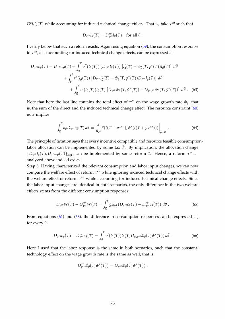
Dexτex lθ(T) while accounting for induced technical change effects. That is, take τen such that

Dτen lθ(T) = Dexτex lθ(T) for all θ .

I verify below that such a reform exists. Again using equation (59), the consumption responseto τen, also accounting for induced technical change effects, can be expressed as

Dτen cθ(T) = Dτen cθ(T) +∫ θ

θv′′(lθ(T)) (Dτen lθ(T))

[l′θ(T) + wθ(T, φ∗(T))lθ(T)

]dθ

+∫ θ

θv′(lθ(T))

[Dτen l′

θ(T) + wθ(T, φ∗(T))Dτen lθ(T)

]dθ

+∫ θ

θv′(lθ(T))lθ(T)

[Dτen wθ(T, φ∗(T)) + Dφ,τen wθ(T, φ∗(T))

]dθ . (63)

Note that here the last line contains the total effect of τen on the wage growth rate wθ , thatis, the sum of the direct and the induced technical change effect. The resource constraint (60)now implies

∫ θ

θhθ Dτen cθ(T) dθ =

ddµ

F(l(T + µτen), φ∗(l(T + µτen)))

∣∣∣∣µ=0

. (64)

The principle of taxation says that every incentive compatible and resource feasible consumption-labor allocation can be implemented by some tax T. By implication, the allocation change{Dτen lθ(T), Dτen cθ(T)}θ∈Θ can be implemented by some reform τ. Hence, a reform τen asanalyzed above indeed exists.Step 3. Having characterized the relevant consumption and labor input changes, we can nowcompare the welfare effect of reform τex while ignoring induced technical change effects withthe welfare effect of reform τen while accounting for induced technical change effects. Sincethe labor input changes are identical in both scenarios, the only difference in the two welfareeffects stems from the different consumption responses:

DτenW(T)− DexτexW(T) =

∫ θ

θgθhθ (Dτen cθ(T)− Dex

τex cθ(T)) dθ . (65)

From equations (61) and (63), the difference in consumption responses can be expressed as,for every θ,

Dτen cθ(T)− Dexτex cθ(T) =

∫ θ

θv′(lθ(T))lθ(T)Dφ,τen wθ(T, φ∗(T)) dθ . (66)

Here I used that the labor response is the same in both scenarios, such that the constant-technology effect on the wage growth rate is the same as well, that is,

Dexτex wθ(T, φ∗(T)) = Dτen wθ(T, φ∗(T)) .

73

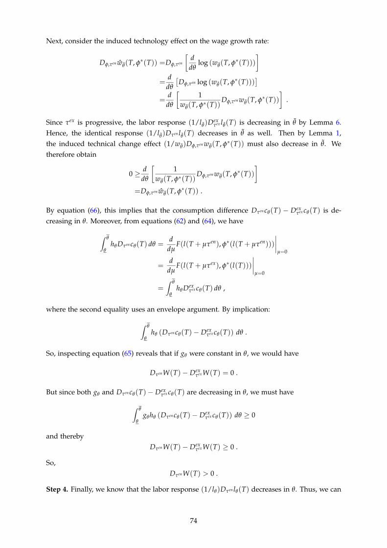
Next, consider the induced technology effect on the wage growth rate:

Dφ,τen wθ(T, φ∗(T)) =Dφ,τen

[ddθ

log (wθ(T, φ∗(T)))]

=ddθ

[Dφ,τen log (wθ(T, φ∗(T)))

]=

ddθ

[1

wθ(T, φ∗(T))Dφ,τen wθ(T, φ∗(T))

].

Since τex is progressive, the labor response (1/lθ)Dexτex lθ(T) is decreasing in θ by Lemma 6.

Hence, the identical response (1/lθ)Dτen lθ(T) decreases in θ as well. Then by Lemma 1,the induced technical change effect (1/wθ)Dφ,τen wθ(T, φ∗(T)) must also decrease in θ. Wetherefore obtain

0 ≥ ddθ

[1

wθ(T, φ∗(T))Dφ,τen wθ(T, φ∗(T))

]=Dφ,τen wθ(T, φ∗(T)) .

By equation (66), this implies that the consumption difference Dτen cθ(T) − Dexτex cθ(T) is de-

creasing in θ. Moreover, from equations (62) and (64), we have

∫ θ

θhθ Dτen cθ(T) dθ =

ddµ

F(l(T + µτen), φ∗(l(T + µτen)))

∣∣∣∣µ=0

=d

dµF(l(T + µτex), φ∗(l(T)))

∣∣∣∣µ=0

=∫ θ

θhθ Dex

τex cθ(T) dθ ,

where the second equality uses an envelope argument. By implication:

∫ θ

θhθ (Dτen cθ(T)− Dex

τex cθ(T)) dθ .

So, inspecting equation (65) reveals that if gθ were constant in θ, we would have

DτenW(T)− DexτexW(T) = 0 .

But since both gθ and Dτen cθ(T)− Dexτex cθ(T) are decreasing in θ, we must have

∫ θ

θgθhθ (Dτen cθ(T)− Dex

τex cθ(T)) dθ ≥ 0

and therebyDτenW(T)− Dex

τexW(T) ≥ 0 .

So,DτenW(T) > 0 .

Step 4. Finally, we know that the labor response (1/lθ)Dτen lθ(T) decreases in θ. Thus, we can

74

again invoke Lemma 6 to obtain that τen must be progressive. We have thereby shown that

DτenW(T) > 0

for a progressive reform τen. So, T ∈ T .Since the preceding reasoning applies to any T ∈ T ex, we have shown that T ex ⊆ T .

D. Proofs and Additional Results for Optimal Taxes

This section contains proofs and additional results for the analysis of optimal taxes in Section6 of the main text. I start by proving Proposition 4 for the general case and then turn to themore detailed analytical results that can be obtained in the CES case.

D.1. General Case

In the general case, optimal taxes are obtained by maximizing wefare W(c, l) subject to the re-source constraint (29) and the incentive compatibility constraint (30). The derivation proceedsalong the following steps: first eliminate consumption from the welfare maximization prob-lem, then derive first-order conditions, use workers’ first-order condition to reintroduce taxrates into the equations, and finally prove the sign conditions for the term TE∗θ at the bottomand the top of the type distribution using directed technical change theory.In the first step the following lemma shows how to eliminate consumption from the welfaremaximization problem.

Lemma 8. The pair of consumption and labor inputs (c, l) satisfies the resource and incentive com-patibility constraints (29) and (30) if and only if c = c∗(l) where c∗(l) = {c∗θ (l)}θ∈Θ is determinedby

c∗θ (l) = F(l, φ∗(l))−∫ θ

θv(lθ)hθ dθ −

∫ θ

θv′(lθ)lθ(1− Hθ)wθ dθ +

∫ θ

θv′(lθ)lθwθ dθ + v(lθ) (67)

for all θ.

Proof. (⇒) I first show that constraints (29) and (30) imply equation (67). For that, writeconsumption as

cθ = cθ +∫ θ

θc′

θdθ .

By the incentive compatibility constraint (30), this implies for all θ:

cθ = cθ +∫ θ

θv′(lθ)(w

′θlθ + wθ l′

θ)

1wθ

dθ

= cθ +∫ θ

θv′(lθ)wθ lθ dθ + v(lθ)− v(lθ) . (68)

75

Combining this with the resource constraint (29), we obtain the following expression for cθ :

cθ = F(l, φ∗(l))−∫ θ

θ

∫ θ

θv′(lθ)wθ lθ dθ hθ dθ −

∫ θ

θv(lθ)hθ dθ + v(lθ) .

Using integration by parts to solve the double integral yields:

cθ = F(l, φ∗(l))−∫ θ

θv′(lθ)wθ lθ(1− Hθ) dθ −

∫ θ

θv(lθ)hθ dθ + v(lθ) .

Inserting this back into equation (68), we obtain:

cθ = F(l, φ∗(l))−∫ θ

θv′(lθ)wθ lθ(1− Hθ) dθ −

∫ θ

θv(lθ)hθ dθ +

∫ θ

θv′(lθ)wθ lθ dθ + v(lθ) ,

which is equation (67) defining the function c∗ above.(⇐) Differentiating c∗ with respect to θ shows immediately that equation (67) implies theincentive compatibility constraint (30). Similarly, after multiplying c∗θ by hθ and integratingover [θ, θ], standard computations show that

∫ θ

θc∗θ (l) dθ = F(l, φ∗(l)) ,

which proves that equation (67) also implies the resource constraint (29).

Proof of Proposition 4. Lemma 8 provides an equivalent representation of resource and incen-tive compatibility constraints, which is explicitly solved for c. Hence, instead of maximizingwelfare subject to the two constraints, we can study the unconstrained maximization of

W(l) := W(c∗(l), l)

with l being the only choice variable. The first part of the proof now uses the first-orderconditions of this unconstrained problem to derive the condition for optimal marginal taxrates provided in Proposition 4.Part 1. The first-order conditions are given by

Dlθ W(l) = 0 for all θ .

We hence study the derivative Dlθ W(l) first. Using the notation for welfare weights introduced

76

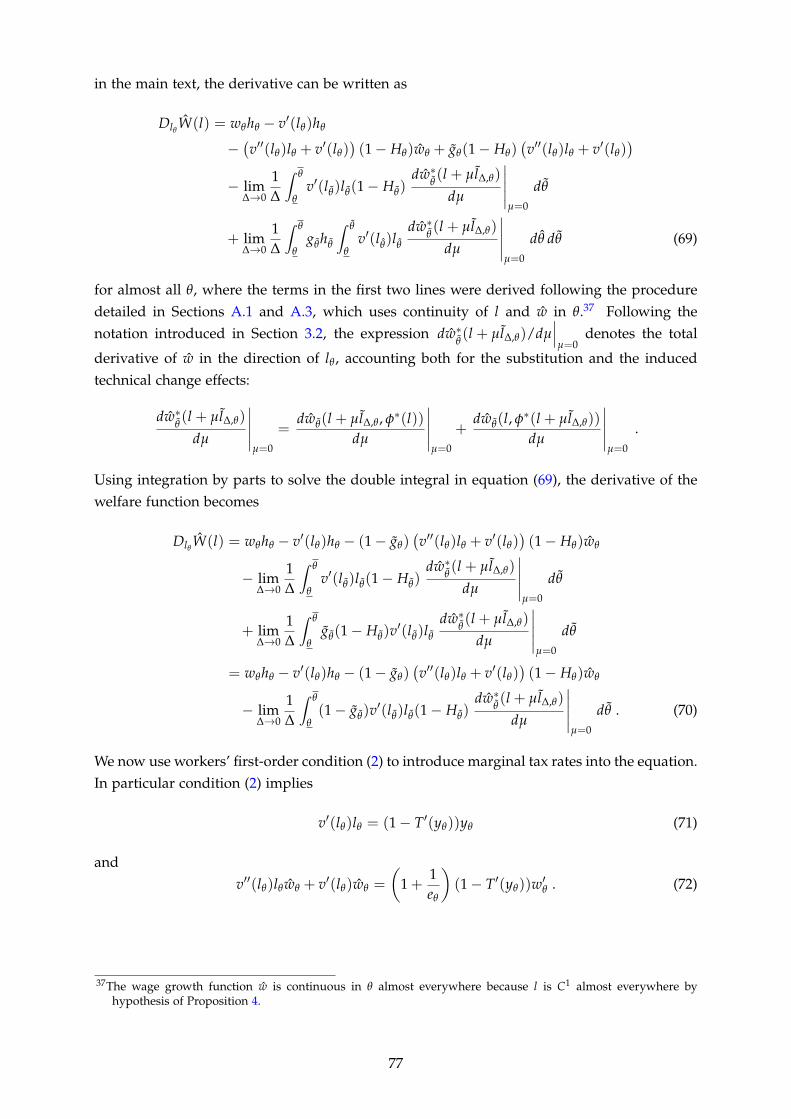
in the main text, the derivative can be written as

Dlθ W(l) = wθhθ − v′(lθ)hθ

−(v′′(lθ)lθ + v′(lθ)

)(1− Hθ)wθ + gθ(1− Hθ)

(v′′(lθ)lθ + v′(lθ)

)− lim

∆→0

1∆

∫ θ

θv′(lθ)lθ(1− Hθ)

dw∗θ(l + µl∆,θ)

dµ

∣∣∣∣∣µ=0

dθ

+ lim∆→0

1∆

∫ θ

θgθhθ

∫ θ

θv′(lθ)lθ

dw∗θ(l + µl∆,θ)

dµ

∣∣∣∣∣µ=0

dθ dθ (69)

for almost all θ, where the terms in the first two lines were derived following the proceduredetailed in Sections A.1 and A.3, which uses continuity of l and w in θ.37 Following thenotation introduced in Section 3.2, the expression dw∗

θ(l + µl∆,θ)/dµ

∣∣∣µ=0

denotes the total

derivative of w in the direction of lθ , accounting both for the substitution and the inducedtechnical change effects:

dw∗θ(l + µl∆,θ)

dµ

∣∣∣∣∣µ=0

=dwθ(l + µl∆,θ , φ∗(l))

dµ

∣∣∣∣∣µ=0

+dwθ(l, φ∗(l + µl∆,θ))

dµ

∣∣∣∣∣µ=0

.

Using integration by parts to solve the double integral in equation (69), the derivative of thewelfare function becomes

Dlθ W(l) = wθhθ − v′(lθ)hθ − (1− gθ)(v′′(lθ)lθ + v′(lθ)

)(1− Hθ)wθ

− lim∆→0

1∆

∫ θ

θv′(lθ)lθ(1− Hθ)

dw∗θ(l + µl∆,θ)

dµ

∣∣∣∣∣µ=0

dθ

+ lim∆→0

1∆

∫ θ

θgθ(1− Hθ)v

′(lθ)lθ

dw∗θ(l + µl∆,θ)

dµ

∣∣∣∣∣µ=0

dθ

= wθhθ − v′(lθ)hθ − (1− gθ)(v′′(lθ)lθ + v′(lθ)

)(1− Hθ)wθ

− lim∆→0

1∆

∫ θ

θ(1− gθ)v

′(lθ)lθ(1− Hθ)dw∗

θ(l + µl∆,θ)

dµ

∣∣∣∣∣µ=0

dθ . (70)

We now use workers’ first-order condition (2) to introduce marginal tax rates into the equation.In particular condition (2) implies

v′(lθ)lθ = (1− T′(yθ))yθ (71)

andv′′(lθ)lθwθ + v′(lθ)wθ =

(1 +

1eθ

)(1− T′(yθ))w′θ . (72)

37The wage growth function w is continuous in θ almost everywhere because l is C1 almost everywhere byhypothesis of Proposition 4.

77

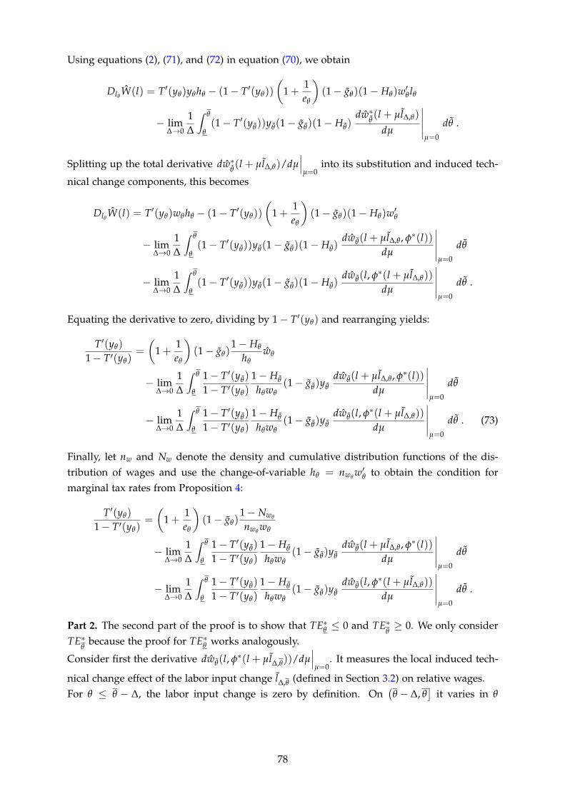
Using equations (2), (71), and (72) in equation (70), we obtain

Dlθ W(l) = T′(yθ)yθhθ − (1− T′(yθ))

(1 +

1eθ

)(1− gθ)(1− Hθ)w′θ lθ

− lim∆→0

1∆

∫ θ

θ(1− T′(yθ))yθ(1− gθ)(1− Hθ)

dw∗θ(l + µl∆,θ)

dµ

∣∣∣∣∣µ=0

dθ .

Splitting up the total derivative dw∗θ(l + µl∆,θ)/dµ

∣∣∣µ=0

into its substitution and induced tech-

nical change components, this becomes

Dlθ W(l) = T′(yθ)wθhθ − (1− T′(yθ))

(1 +

1eθ

)(1− gθ)(1− Hθ)w′θ

− lim∆→0

1∆

∫ θ

θ(1− T′(yθ))yθ(1− gθ)(1− Hθ)

dwθ(l + µl∆,θ , φ∗(l))dµ

∣∣∣∣∣µ=0

dθ

− lim∆→0

1∆

∫ θ

θ(1− T′(yθ))yθ(1− gθ)(1− Hθ)

dwθ(l, φ∗(l + µl∆,θ))

dµ

∣∣∣∣∣µ=0

dθ .

Equating the derivative to zero, dividing by 1− T′(yθ) and rearranging yields:

T′(yθ)

1− T′(yθ)=

(1 +

1eθ

)(1− gθ)

1− Hθ

hθwθ

− lim∆→0

1∆

∫ θ

θ

1− T′(yθ)

1− T′(yθ)

1− Hθ

hθwθ(1− gθ)yθ

dwθ(l + µl∆,θ , φ∗(l))dµ

∣∣∣∣∣µ=0

dθ

− lim∆→0

1∆

∫ θ

θ

1− T′(yθ)

1− T′(yθ)

1− Hθ

hθwθ(1− gθ)yθ

dwθ(l, φ∗(l + µl∆,θ))

dµ

∣∣∣∣∣µ=0

dθ . (73)

Finally, let nw and Nw denote the density and cumulative distribution functions of the dis-tribution of wages and use the change-of-variable hθ = nwθ

w′θ to obtain the condition formarginal tax rates from Proposition 4:

T′(yθ)

1− T′(yθ)=

(1 +

1eθ

)(1− gθ)

1− Nwθ

nwθwθ

− lim∆→0

1∆

∫ θ

θ

1− T′(yθ)

1− T′(yθ)

1− Hθ

hθwθ(1− gθ)yθ

dwθ(l + µl∆,θ , φ∗(l))dµ

∣∣∣∣∣µ=0

dθ

− lim∆→0

1∆

∫ θ

θ

1− T′(yθ)

1− T′(yθ)

1− Hθ

hθwθ(1− gθ)yθ

dwθ(l, φ∗(l + µl∆,θ))

dµ

∣∣∣∣∣µ=0

dθ .

Part 2. The second part of the proof is to show that TE∗θ ≤ 0 and TE∗θ≥ 0. We only consider

TE∗θ

because the proof for TE∗θ works analogously.

Consider first the derivative dwθ(l, φ∗(l + µl∆,θ))/dµ∣∣∣µ=0

. It measures the local induced tech-

nical change effect of the labor input change l∆,θ (defined in Section 3.2) on relative wages.For θ ≤ θ − ∆, the labor input change is zero by definition. On

(θ − ∆, θ

]it varies in θ

78

according to1

l∆,θ,θ

dl∆,θ,θ

dθ=

2∆2∆(θ − θ + ∆)

=1

θ − θ + ∆≥ 1

∆.

Hence, given the optimal labor input l, we can find an ε > 0 such that for all ∆ < ε and forall θ ∈ (θ − ∆, θ):

1l∆,θ,θ

dl∆,θ,θ

dθ≥ 1

lθ

dlθ

dθ.38

So, for ∆ < ε, the relative labor input change l∆,θ,θ/lθ increases in θ. Thus, by Lemma 1, weobtain that

dwθ(l, φ∗(l + µl∆,θ))

dµ

∣∣∣∣∣µ=0

≥ 0

for all θ if ∆ < ε. Hence, for ∆ < ε,

∫ θ

θ

1− T′(yθ)

1− T′(yθ)

1− Hθ

hθwθ(1− gθ)yθ

dwθ(l, φ∗(l + µl∆,θ))

dµ

∣∣∣∣∣µ=0

dθ ≥ 0

and therefore

TE∗θ= lim

∆→0

1∆

∫ θ

θ

1− T′(yθ)

1− T′(yθ)

1− Hθ

hθwθ(1− gθ)yθ

dwθ(l, φ∗(l + µl∆,θ))

dµ

∣∣∣∣∣µ=0

dθ ≥ 0 .

D.2. CES Case

To derive expression (32) for optimal tax rates in Proposition 5, I start by specializing the termsTE∗θ and SE∗θ to the CES case.

Lemma 9. Suppose the conditions of Proposition 4 are satisfied and F and Φ take the CES formintroduced in Section 3.4. Then, the terms TE∗θ and SE∗θ take the following form for almost every θ:

SE∗θ = (1− gθ)γCES −

(1 +

1eθ

)1− Hθ

hθ(1− gθ)lθγCES (74)

TE∗θ = (1− gθ)ρCES −

(1 +

1eθ

)1− Hθ

hθ(1− gθ)lθρCES . (75)

Proof. I focus on the expression for TE∗θ , because the derivation of SE∗θ is analogous with γCES

in the place of ρCES.The central step is to obtain an expression for the derivative of wθ in TE∗θ . From equation (13)we obtain

wθ =σ− 1

σκθ +

σ− 1σ

φθ −1σ

lθ −1σ

hθ (76)

and from equation (41):

φ∗θ=

σ− 1(δ− 1)σ + 1

(κθ + lθ + hθ

). (77)

38Here we use that by hypothesis l′θ exists on some right neighborhood of θ and lim supθ→θ l′θ < ∞.

79

Hence, the partial effect of the perturbation l∆,θ on wθ is

dwθ(l + µl∆,θ , φ∗(l))dµ

∣∣∣∣∣µ=0

= − 1σ

ddµ

( lθ + µl∆,θ,θ)

∣∣∣∣µ=0

= − 1σ

ddµ

l′θ+ µl′∆,θ,θ

lθ + µl∆,θ,θ

∣∣∣∣∣µ=0

= γCES

(l′∆,θ,θ

lθ

− lθ

l∆,θ,θ

lθ

).

Analogously, the induced technical change effect is given by

dwθ(l, φ∗(l + µl∆,θ))

dµ

∣∣∣∣∣µ=0

=(σ− 1)2

(δ− 1)σ2 + σ

ddµ

( lθ + µl∆,θ,θ)

∣∣∣∣µ=0

= ρCES

(l′∆,θ,θ

lθ

− lθ

l∆,θ,θ

lθ

).

Using the last expression and the definition of l∆,θ , the term TE∗θ becomes

TE∗θ = lim∆→0

1∆2

∫ θ

θ−∆

1− T′(yθ)

1− T′(yθ)

1− Hθ

hθwθ(1− gθ)wθρCES

(1− lθ(θ − θ + ∆)

)dθ

+1

∆2

∫ θ+∆

θ

1− T′(yθ)

1− T′(yθ)

1− Hθ

hθwθ(1− gθ)wθρCES

(−1− lθ(θ − θ + ∆)

)dθ .

Applying L’Hospital’s rule yields:

TE∗θ = lim∆→0

12∆

1− T′(yθ−∆)

1− T′(yθ)

1− Hθ−∆

hθwθ(1− gθ−∆)wθ−∆ρCES

− 12∆

∫ θ

θ−∆

1− T′(yθ)

1− T′(yθ)

1− Hθ

hθwθ(1− gθ)wθρCES lθ dθ

− 12∆

1− T′(yθ+∆)

1− T′(yθ)

1− Hθ+∆

hθwθ(1− gθ+∆)wθ+∆ρCES

− 12∆

∫ θ+∆

θ

1− T′(yθ)

1− T′(yθ)

1− Hθ

hθwθ(1− gθ)wθρCES lθ dθ .

Rearranging and replacing marginal retention rates by workers’ first-order condition (2), weobtain:

TE∗θ = lim∆→0

12∆

ρCES[

v′(lθ−∆

v′(lθ)

1− Hθ−∆

hθ(1− gθ−∆)−

v′(lθ+∆

v′(lθ)

1− Hθ+∆

hθ(1− gθ+∆)

]− 1

2∆

∫ θ

θ−∆

v′(lθ

v′(lθ)

1− Hθ

hθ(1− gθ)ρ

CES lθ dθ

− 12∆

∫ θ+∆

θ

v′(lθ

v′(lθ)

1− Hθ

hθ(1− gθ)ρ

CES lθ dθ .

80

Next, we apply L’Hospital’s rule a second time and obtain:

TE∗θ = −v′′(lθ)

v′(lθ)

1− Hθ

hθ(1− gθ)l′θρCES + (1− gθ)ρ

CES +1− Hθ

hθg′θρCES − 1− Hθ

hθ(1− gθ)lθρCES .

Using the definition of the elasticity eθ yields:

TE∗θ = − 1eθ

1− Hθ

hθ(1− gθ)lθρCES + (1− gθ)ρ

CES +1− Hθ

hθg′θρCES − 1− Hθ

hθ(1− gθ)lθρCES .

Finally, it is straightforward to show that

g′θ = (gθ − gθ)hθ

1− Hθ.

Inserting this into the previous expression for TE∗θ , we obtain:

TE∗θ = − 1eθ

1− Hθ

hθ(1− gθ)lθρCES + (1− gθ)ρ

CES + (gθ − gθ)ρCES − 1− Hθ

hθ(1− gθ)lθρCES

and after rearranging:

TE∗θ = (1− gθ)ρCES −

(1 +

1eθ

)1− Hθ

hθ(1− gθ)lθρCES ,

which is the desired expression.

Besides providing an important step in the derivation of equation (32), Lemma 9 allows torevisit the sign of TE∗θ at the bottom and the top of the type distribution. In the general case,Proposition 4 shows that the induced technical change term is weakly positive at the top andweakly negative at the bottom. For the CES case, Lemma 9 implies39

TE∗θ= (1− gθ)ρ

CES > 0

andTE∗θ = (1− gθ)ρ

CES < 0 .

Hence, in the CES case the sign restrictions on the induced technical change term hold strictly.Moreover, Lemma 9 implies the opposite signs for the substitution term at the top and bottomtypes:

SE∗θ= (1− gθ)γ

CES > 0

andSE∗θ = (1− gθ)γ

CES < 0 .

Hence, at the highest and lowest income levels, induced technical change and within-technologysubstitution effects push optimal marginal tax rates in opposing directions. Adding the two

39This again assumes that l′θ exists on some left (right) neighborhood of θ (θ) and lim supθ→θ l′θ < ∞(lim infθ→θ l′θ > −∞) under the optimal tax, as in the second part of Proposition 4. Moreover, the strict in-equalities below require that marginal welfare weights are strictly decreasing at the optimum over parts oftype distribution.

81

up yields:SE∗

θ+ TE∗

θ= (1− gθ)(γ

CES + ρCES)

andSE∗θ + TE∗θ = (1− gθ)(γ

CES + ρCES) .

The total effect of endogenous wage responses therefore depends on whether condition (19)for strong relative bias from Section 4 is satisfied: if and only if γCES + ρCES ≥ 0, the adjust-ment of optimal marginal tax rates for endogeneity of the wage distribution is positive at thetop and negative at the bottom.Since the partial equilibrium term PE∗θ is zero at the top and bottom types, these insightsdirectly translate into conclusions about the sign of the optimal marginal tax rate at the topand the bottom of the income distribution. The optimal marginal tax is positive at the top ifand only if there is strong relative bias of technology, providing a counterpart to the negativemarginal top tax result in Stiglitz (1987). Analogously, the optimal marginal tax is negative atthe bottom if and only if there is strong bias.With the expressions from Lemma 9, we are now in a position to derive equation (32).

Proof of Proposition 5. We start with equation (73) from the proof of Proposition 4 and replaceSE∗θ and TE∗θ by the expressions from Lemma 9. This yields:

T′(yθ)

1− T′(yθ)=

(1 +

1eθ

)1− Hθ

hθ(1− gθ)wθ (78)

+ (γCES + ρCES)

[(1− gθ)−

(1 +

1eθ

)1− Hθ

hθ(1− gθ)lθ

]=

(1 +

1eθ

)1− Hθ

hθ(1− gθ)

(wθ − (γCES + ρCES)lθ

)(79)

+ γCES(1− gθ) + ρCES(1− gθ) . (80)

The wage growth rate wθ can be computed from equations (76) and (77) as

wθ = (1 + γCES + ρCES)κθ + (γCES + ρCES)hθ + (γCES + ρCES)lθ .

Using this in the previous expression for marginal tax rates yields

T′(yθ)

1− T′(yθ)=

(1 +

1eθ

)1− Hθ

hθ(1− gθ)

[(1 + γCES + ρCES)κθ + (γCES + ρCES)hθ

]+ γCES(1− gθ) + ρCES(1− gθ) .

Now we use the definition of β,

βθ := κ1+γCES+ρCES

θ hγCES+ρCES

θ ,

to note that(1 + γCES + ρCES)κθ + (γCES + ρCES)hθ = βθ

82

and hence

T′(yθ)

1− T′(yθ)=

(1 +

1eθ

)1− Hθ

hθ(1− gθ)βθ + γCES(1− gθ) + ρCES(1− gθ) .

Finally, with the change-of-variable hθ = bβθβ′θ , we obtain equation (32):

T′(yθ)

1− T′(yθ)=

(1 +

1eθ

)1− Bβθ

bβθβθ

(1− gθ) + γCES(1− gθ) + ρCES(1− gθ) .

Finally, I provide an alternative expression for optimal marginal tax rates in the CES case,which allows for an interpretation of directed technical change effects via their effect on theaggregate labor supply elasticity εR

θ (see Appendix C.4).

Proposition 7. Suppose the conditions of Proposition 4 are satisfied and F and Φ take the CES formintroduced in Section 3.4. Additionally, let (γCES + ρCES)εw

θ < 1 at the optimal tax T. Then, theconditions for optimal marginal tax rates can be written as

T′(y)1− T′(y)

=1

εRθy

1−My

myy(1− gθy) + γCES(1− gθy) + ρCES(1− gθy) , (81)

where

εRθy(T, l, w) :=

εRθy(T, l, w)

1− (γθy,θy + ρθy,θy)εwθy(T, l, w)

denotes the elasticity of aggregate labor supply of type θ with respect to the marginal retention rate (seeAppendix C.4); all variables are evaluated at equilibrium under the optimal tax T; M and m denotethe cumulative distribution and the density function of y at the optimum; and θy denotes the type ofworkers who earn income y at the optimum.

Proof. To derive equation (81), we start from equation (80) and replace lθ by εwθ wθ :

T′(yθ)

1− T′(yθ)=

(1 +

1eθ

)1− Hθ

hθ(1− gθ)wθ

(1− (γCES + ρCES)εw

θ

)+γCES(1− gθ)+ ρCES(1− gθ) .

Using my and My to denote density and cumulative distribution function of income, a change-of-variable implies hθ = myθ

y′− θ. Using this in the previous expression for marginal tax rates,

83

we obtain:

T′(yθ)

1− T′(yθ)=

(1 +

1eθ

)1−Myθ

myθyθ

1wθ + lθ

(1− gθ)wθ

(1− (γCES + ρCES)εw

θ

)+ γCES(1− gθ) + ρCES(1− gθ)

=

(1 +

1eθ

)1−Myθ

myθyθ

1wθ(1 + εw

θ )(1− gθ)wθ

(1− (γCES + ρCES)εw

θ

)+ γCES(1− gθ) + ρCES(1− gθ)

=

(1 +

1eθ

)1−Myθ

myθyθ

11 + εw

θ

(1− gθ)(

1− (γCES + ρCES)εwθ

)+ γCES(1− gθ) + ρCES(1− gθ) .

From the expression for εwθ and εR

θ in Section 3.2, it is straightforward to show that(1 +

1eθ

)1

1 + εwθ

=1

εRθ

,

and hence

T′(yθ)

1− T′(yθ)=

1− (γCES + ρCES)εwθ

εRθ

1−Myθ

myθyθ

(1− gθ) + γCES(1− gθ) + ρCES(1− gθ) .

By definition of the aggregate elasticity εRθ (see Appendix C.4), this yields equation (81) from

Proposition 5:

T′(yθ)

1− T′(yθ)=

1εR

θ

1−Myθ

myθyθ

(1− gθ) + γCES(1− gθ) + ρCES(1− gθ) .

Equation (81) offers an alternative perspective on the role of directed technical change in theCES case. It extends the expression in Proposition 3 of Sachs et al. (2019) to account fordirected technical change.The adjustment term ρCES(1− gθy) is the same as in equation (32) and does not provide anynew insights. As described in the main text, it calls for a progressive adjustment of marginaltax rates.The second place in equation (81) where induced technical change elasticities appear is theaggregate labor supply elasticity εR

θ . This elasticity measures the response of labor supply oftype θ to an increase in the marginal retention rate when taking into account the change intype θ’s wage induced by the labor supply response. The change in type θ’s wage is modifiedby directed technical change effects. Specifically, when labor supply of type θ falls due to anincrease in the marginal tax rate, directed technical change amplifies the fall in labor supplyby reducing the wage of type θ. In this way, directed technical change effects magnify thelabor supply response to marginal tax changes, which leads to a downwards adjustment ofoptimal marginal tax rates.

84

D.3. Exogenous Technology Planner

As described in the main text, the exogenous technology planner believes that the economyworks according to all reduced form equations from Section 3.1 with the exception of thecondition for the equilibrium technology (7). Instead of following equation (7), the exogenoustechnology planner believes that technology remains fixed at its equilibrium value under agiven tax T, φ∗(l(T)). The idea is that the planner observes the economy under the tax Twhen computing optimal taxes and believes technology to be exogenous.The exogenous technology planner’s optimal tax Tex

Tthen satisfies the conditions provided by

the following Lemma.

Lemma 10. Suppose the conditions of Proposition 4 are satisfied and F and Φ take the CES formintroduced in Section 3.4. Suppose equilibrium variables are determined according to the reduced formequations (2), (1), (6), and (8), plus the (exogenous) technology equation

φ∗(l) = φ∗(l(T)) = argmaxφ∈Φ

F(l(T), φ) ∀l ,

where T is a given initial tax function.Then, at almost every type θ, the exogenous technology planner’s preferred tax Tex

Tsatisfies the following

conditions.Tex′

T(yθ)

1− Tex′T

(yθ)=

(1 +

1eθ

) 1− Bβθ

bβθβθ

(1− gθ) + γCES(1− gθ) ,

where all variables satisfy the equations listed above under the tax TexT

; the function β : θ 7→ βθ isgiven by

βθ := κ1+γCES

θ hγCES

θ

(φ∗(T)

)1+γCES

∀ θ ;

and B and b are the cumulative distribution and the density function of β.

Proof. It can be verified that all steps in the proof of Proposition 4 hold for the case of theexogenous technology planner when imposing

dwθ(l, φ∗(l + µl∆,θ))

dµ

∣∣∣∣∣µ=0

= 0 .

With this constraint, we can derive a counterpart to equation (73) for the exogenous technologyplanner:

T′(yθ)

1− T′(yθ)=

(1 +

1eθ

)(1− gθ)

1− Hθ

hθwθ − SE∗θ .

Using Lemma 9 to replace SE∗θ , we obtain:

T′(yθ)

1− T′(yθ)=

(1 +

1eθ

)1− Hθ

hθ(1− gθ)wθ

+ γCES[(1− gθ)−

(1 +

1eθ

)1− Hθ

hθ(1− gθ)lθ

]=

(1 +

1eθ

)1− Hθ

hθ(1− gθ)

(wθ − γCES lθ

)+ γCES(1− gθ) .

85

From the perspective of the exogenous technology planner, the wage growth rate is now givenby

wθ = (1 + γCES)κθ + (1 + γCES)φ∗θ (T) + γCEShθ + γCES lθ ,

where φ∗θ (T) denotes the growth rate of technology that prevails in equilibrium under theinitial tax system T. Using this in the previous expression for the exogenous technologyplanner’s optimal tax rates and applying the definition of β yields:

T′(yθ)

1− T′(yθ)=

(1 +

1eθ

)1− Hθ

hθ(1− gθ)βθ + γCES(1− gθ) .

With the change of variable hθ = bβθβ′θ , we obtain equation (33),

T′(yθ)

1− T′(yθ)=

(1 +

1eθ

) 1− Bβθ

bβθβθ

(1− gθ) + γCES(1− gθ) ,

which completes the proof.

D.4. Comparison between Endogenous and Exogenous Technology Planner

As discussed in the main text, the optimal tax conditions of the endogenous and the exogenoustechnology planner feature two differences. First, the exogenous technology planner neglectsthe progressive term ρCES(1− gθ). Second, he uses β instead of β to measure the degree ofexogenous inequality in the economy. Here I show that the exogenous technology plannerthereby overestimates exogenous inequality: the function β progresses at a higher rate in θ

than the function β, such that equation (34) holds.First, let l be the equilibrium labor input under the initial tax system T. Then, by constructionthe growth rates of β and β must satisfy

βθ = wθ(l, φ∗(l))− (γCES + ρCES)lθ

andβθ = wθ(l, φ∗(l))− γCES lθ .

Moreover, if we assume (as is done in the main text) that the rate of progressivity of the initialtax schedule T is strictly below one everywhere, then equation (10) implies that εw

θ > 0 andhence lθ = εw

θ wθ(l, φ∗(l)) > 0 for all θ. Combining this with the expressions for βθ and βθ ,we find that βθ < βθ . Intuitively, since labor supply increases in the skill index under taxT, technology under this tax must be skill-biased. The exogenous technology planner falselybelieves this skill bias to be exogenous and to persist irrespective of changes in labor supply.Thereby, he overestimates the degree of exogenous inequality in the economy.Now use a change-of-variable to obtain

bβθβθ =

fθ

βθ

>fθ

βθ

= bβθβθ ,

86

and hence1− Bβθ

bβθβθ

<1− Bβθ

bβθβθ

,

which proves equation (34) in the main text.

Comparison in the Lower Tail

Proof of Corollary 3. We first show that the two inequalities of Corollary 3 hold at the lowesttype θ. Since gθ = 1, equation (32) from Proposition 5 implies

T′(yθ(T))1− T′(yθ(T))

= γCES(1− gθ) + ρCES(1− gθ) ,

while equation (33) from Lemma 10 implies

Tex′T

(yθ(TexT))

1− Tex′T

(yθ(TexT))

= γCES(1− gθ) .

With ρCES > 0 and gθ > 1 (because welfare weights are strictly decreasing by hypothesis) theinequality

T′(yθ(T)) < Tex′T (yθ(Tex

T ))

follows.Moreover, if γCES + ρCES > 0, the previous expression for optimal marginal tax rates withendogenous technology effects produces the second inequality

T′(yθ(T)) < 0 .

Finally, under the conditions of the corollary, the expressions for optimal marginal tax rates inequations (32) and (33) are continuous. Thus, the previous inequalities extend to some rightneighborhoods of θ, which completes the proof.

Comparison in the Upper Tail

Proof of Corollary 4. As described in the main text, we trace the Pareto property of the (uppertail of the) income distribution under tax T back to the distribution of the exogenous inequalitymeasure β. Inserting this distribution into the optimal tax formula (32) from Proposition 5 thenyields the desired result.First, by two changes-of-variable we obtain

1− Bβθ

bβθβθ

=1− Hθ

hθβθ =

1−Myθ

myθyθ

βθ

yθ, (82)

where all incomes are assessed at the given tax T. Now we use

yθ = wθ + lθ = (1 + εwθ )wθ

87

to express the growth rate of income as a function of the growth rate of wages under tax, againassessing all endogenous variables at equilibrium under the given tax T. For βθ we obtain

βθ = wθ − (γCES + ρCES)lθ =(

1− (γCES + ρCES)εwθ

)wθ .

It follows thatβθ

yθ=

1− (γCES + ρCES)εwθ

1 + εwθ

and, with equation (82),

1− Bβθ

bβθβθ

=1−Myθ

myθyθ

1− (γCES + ρCES)εwθ

1 + εwθ

, (83)

where incomes and the labor supply elasticity εwθ are assessed under the tax T. In particular,

εwθ =

(1− PT(yθ))eθ

1 + eθ PT(yθ).

Since the tax T features a constant top tax rate, we have limθ→θ PT(yθ) = 0 and hence

limθ→θ

εwθ = eθ = e ,

where the last equality reflects the assumption that the disutility of labor is iso elastic. More-over, we know by hypothesis that

limθ→θ

1−Myθ

myθyθ

=1a

.

Combining these limits, we obtain

limθ→θ

1− Bβθ

bβθβθ

= limθ→θ

1−Myθ

myθyθ

1− (γCES + ρCES)εwθ

1 + εwθ

=1− (γCES + ρCES)e

a(1 + e).

In words, from the observed Pareto tail of the income distribution under tax T we can inferthat the exogenous inequality measure β must also have a Pareto tail with tail parametergiven by the previous equation. Using this parameter in the optimal tax equation (32) fromProposition 5, we obtain the following expression for the optimal marginal tax rate in theupper tail of the income distribution:

limθ→θ

T′(yθ)

1− T′(yθ)=

(1 +

1e

)1− (γCES + ρCES)e

a(1 + e)(1− gtop) + γCES(1− gtop) + ρCES(1− gtop)

=1− gtop

ae+

a− 1a

γCES(1− gtop) +a− 1

aρCES(1− gtop) ,

where gtop is the asymptotic welfare weight defined in the Corollary.

To precisely identify the role of endogenously directed technical change, I compare the optimalmarginal tax in Corollary 4 to the one computed by the exogenous technology planner. The

88

exogenous technology planner again observes the economy under an initial tax T and believesthat technology φ∗ remains fixed at its initial level φ∗(T), irrespectively of the tax system. Now,in analogy to the conditions of Corollary 4, the initial tax T has a constant marginal top taxrate and the upper tail of the income distribution has a Pareto shape under the initial tax.

Corollary 6. Suppose the conditions of Proposition 4 are satisfied and F and Φ take the CES formintroduced in Section 3.4. Suppose equilibrium variables were determined by the reduced form equations(2), (1), (6), and (8), and by the (exogenous) technology equation

φ∗(l) = φ∗(l(T)) = argmaxφ∈Φ

F(l(T), φ) ∀l ,

where T is a given initial tax function with T′(y) = τtop for all y ≥ y and some threshold y.Moreover, assume that under the tax T the income distribution satisfies

limθ→θ

1−Myθ

myθyθ

=1a

for some a > 1. Finally, let the disutility of labor be iso elastic with eθ = e for all θ, and welfare weightssatisfy

limθ→θ

gθ = gtop

at the exogenous technology planner’s preferred tax.Then, the exogenous technology planner’s preferred tax Tex

Tsatisfies

limθ→θ

Tex′T

(yθ)

1− Tex′T

(yθ)=

1− gtop

ae+

a− 1a

γCES(1− gtop) .

Proof. The corollary can be derived from Lemma 10 in the same way as Corollary 4 is derivedfrom Proposition 5. In particular, consider first the implications of the Pareto shape of theincome distribution under tax T for the exogenous inequality measure β. Using changes-of-variable, we obtain

1− Bβθ

bβθβθ

=1− Hθ

hθβθ =

1−Myθ

myθyθ

βθ

yθ, (84)

where all incomes are assessed at the given tax T. The exogenous technology planner’s mea-sure of exogenous inequality β now evolves over the type space according to

βθ = wθ − γCES lθ =(

1− γCESεwθ

)wθ ,

whileyθ = wθ + lθ = (1 + εw

θ )wθ ,

where all endogenous variables are assessed at equilibrium under the given tax T.40 Combin-

40Note that under the initial tax T the exogenous and the endogenous planner agree about the equilibrium andin particular about the equilibrium technology. Hence, there is no need to distinguish the equilibrium valuesof the endogenous variables under tax T as perceived by the exogenous technology planner and their trueequilibrium values.

89

ing the previous expressions, we find that

βθ

yθ=

1− γCESεwθ

1 + εwθ

and, with equation (84),1− Bβθ

bβθβθ

=1−Myθ

myθyθ

1− γCESεwθ

1 + εwθ

, (85)

where incomes and the labor supply elasticity εwθ are assessed under the tax T. Inserting

this expression into equation (33) for optimal marginal tax rates computed by the exogenoustechnology planner and taking limits yields41

limθ→θ

Tex′T

(yθ)

1− Tex′T

(yθ)=

(1 +

1e

)1− γCESea(1 + e)

(1− gtop) + γCES(1− gtop)

=1− gtop

ae+

a− 1a

γCES(1− gtop) .

E. Additional Explanations and Results for the Quantification

In the following I provide details on the calibration described in Section 7.1 of the main text.For the calibration I use the CES version of the model and assume iso-elastic disutility of labor(see Section 3.4).

E.1. Calibration of Directed Technical Change Effects

The parameter ρCES, which controls the strength of directed technical change effects, is cali-brated on the basis of the empirical estimates summarized in Table 1. The long-run estimatesin Table 1 (10 years or more) are equated with the sum of within-technology substitutionand directed technical change elasticities γCES + ρCES. The short-run estimate (2 years, fromCarneiro et al. (2019)) is equated with γCES, in line with other short-run estimates as discussedin the main text.Here, I give a brief overview over each of the studies used in Table 1 and explain how I obtainthe estimates in the last column of Table 1 from the respective studies.

Carneiro et al. (2019) Carneiro et al. (2019) estimate the responses of relative supply andrelative wages of college versus non-college workers to plausibly exogenous college openingsin Norwegian municipalities in the 1970s, using synthetic control methods. They find thatrelative supply in a municipality starts rising shortly after the college opening and follows anupwards trend throughout the observation period of up to 17 years, compared to the syntheticcontrol municipality. The relative wage first declines and then reverses its trend, surpassing

41The limit computations are analogous to those in the proof of Corollary 4, so I omit the details here.

90

the relative wage in the control municipality slightly more than 10 years after the collegeopening (see Figures 4 and 5 in Carneiro et al. 2019).The numbers in Table 1 are derived from the estimates presented in Carneiro et al. (2019) asfollows. First, measuring relative supply and relative wage changes two years after a collegeopening, Carneiro et al. (2019) estimate an elasticity of the relative wage with respect to relativesupply of −0.549, reported in column 1 of their Table 2. This produces the first row of Table1 in the present paper.Second, Figures 4 and 5 imply that after 10 years, relative wages in the treated municipalitiesand their synthetic controls were equal. Hence, when measured after 10 years, there is a zeroeffect of the exogenous relative supply increase in the relative wage, leading to the secondrow of Table 1 in the present paper.Finally, the third row of Table 1 is obtained from the plots presented in Figure 4 in Carneiroet al. (2019) as follows. The figure shows that after 17 years, the log change in the relativewage, compared to the synthetic control municipality, is

log(

w17c

w17nc

)− log

(w0

cw0

nc

)≈ 0.02 .

At the same time, the log change in the share of college workers in the total workforce was

log(

l17c

l17c + l17

nc

)− log

(l0c

l0c + l0

nc

)≈ 0.04 .

To map this change into the change in the ratio of college over non-college workers, I rewritethe log change as follows:

log(

l17c

l17c + l17

nc

)− log

(l0c

l0c + l0

nc

)= log(l17

c )− log(l17nc)− log(l0

c ) + log(l0nc)

− log(l17c + l17

nc) + log(l17nc) + log(l0

c + l0nc)− log(l0

nc) .

Carneiro et al. (2019) report that the share of college workers was close to zero in most of thetreated municipalities at the beginning of the observation period and still small at the end ofthe period. Hence, I apply the approximations

log(l17c + l17

nc)− log(l17nc) ≈ log(l0

c + l0nc)− log(l0

nc) ≈ 0

to obtain

log(

l17c

l17c + l17

nc

)− log

(l0c

l0c + l0

nc

)≈ log(l17

c )− log(l17nc)− log(l0

c ) + log(l0nc) ≈ 0.04 .

Finally, relating the change in relative supply to the change in relative wages, I obtain

log(

w17c

w17nc

)− log

(w0

cw0

nc

)log(

l17c

l17nc

)− log

(l0c

l0nc

) ≈ 0.05 ,

91

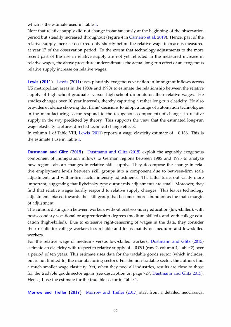
which is the estimate used in Table 1.Note that relative supply did not change instantaneously at the beginning of the observationperiod but steadily increased throughout (Figure 4 in Carneiro et al. 2019). Hence, part of therelative supply increase occurred only shortly before the relative wage increase is measuredat year 17 of the observation period. To the extent that technology adjustments to the morerecent part of the rise in relative supply are not yet reflected in the measured increase inrelative wages, the above procedure underestimates the actual long-run effect of an exogenousrelative supply increase on relative wages.

Lewis (2011) Lewis (2011) uses plausibly exogenous variation in immigrant inflows acrossUS metropolitan areas in the 1980s and 1990s to estimate the relationship between the relativesupply of high-school graduates versus high-school dropouts on their relative wages. Hestudies changes over 10 year intervals, thereby capturing a rather long-run elasticity. He alsoprovides evidence showing that firms’ decisions to adopt a range of automation technologiesin the manufacturing sector respond to the (exogenous component) of changes in relativesupply in the way predicted by theory. This supports the view that the estimated long-runwage elasticity captures directed technical change effects.In column 1 of Table VIII, Lewis (2011) reports a wage elasticity estimate of −0.136. This isthe estimate I use in Table 1.

Dustmann and Glitz (2015) Dustmann and Glitz (2015) exploit the arguably exogenouscomponent of immigration inflows to German regions between 1985 and 1995 to analyzehow regions absorb changes in relative skill supply. They decompose the change in rela-tive employment levels between skill groups into a component due to between-firm scaleadjustments and within-firm factor intensity adjustments. The latter turns out vastly moreimportant, suggesting that Rybcinsky type output mix adjustments are small. Moreover, theyfind that relative wages hardly respond to relative supply changes. This leaves technologyadjustments biased towards the skill group that becomes more abundant as the main marginof adjustment.The authors distinguish between workers without postsecondary education (low-skilled), withpostsecondary vocational or apprenticeship degrees (medium-skilled), and with college edu-cation (high-skilled). Due to extensive right-censoring of wages in the data, they considertheir results for college workers less reliable and focus mainly on medium- and low-skilledworkers.For the relative wage of medium- versus low-skilled workers, Dustmann and Glitz (2015)estimate an elasticity with respect to relative supply of −0.091 (row 2, column 4, Table 2) overa period of ten years. This estimate uses data for the tradable goods sector (which includes,but is not limited to, the manufacturing sector). For the non-tradable sector, the authors finda much smaller wage elasticity. Yet, when they pool all industries, results are close to thosefor the tradable goods sector again (see description on page 727, Dustmann and Glitz 2015).Hence, I use the estimate for the tradable sector in Table 1.

Morrow and Trefler (2017) Morrow and Trefler (2017) start from a detailed neoclassical

92

model of international trade building on Eaton and Kortum (2002). They estimate their modelon sectoral factor input and price data for a cross-section of 38 countries in 2006. Countryselection is driven by data availability in the World Input Output Database. Labor is parti-tioned into skilled and unskilled labor. Skilled workers are those with at least some tertiaryeducation, unskilled workers are those without.In the model, the relative wage between skilled and unskilled workers in each country isdetermined by the relative labor input and exogenous factor-augmenting productivity. Toseparately identify factor-augmenting productivity and the elasticity of substitution betweenlabor types, Morrow and Trefler (2017) augment their model’s equilibrium conditions by adirected technical change equation similar to equation (41). Unfortunately, their approachrequires to fix the technology substitution parameter δ exogenously. In their directed technicalchange equation, they (implicitly) assume δ = 1. Given a value for δ, the directed technicalchange equation and the equation for relative wages at given technology identify the elasticityof substitution σ.In their most elaborate estimation, Morrow and Trefler (2017) find a value for σ of 1.89, whichtranslates into a wage elasticity at exogenous technology (or, short-run wage elasticity) of−1/1.89 = 0.53. This is the first value from Morrow and Trefler (2017) I use in Table 1.Combining relative wage and directed technical change equations, the total wage elasticity,including directed technical change effects, is then obtained as σ − 2 = −0.11, the secondestimate from Morrow and Trefler (2017) reported in Table 1.Relative to the other studies listed in Table 1, a major shortcoming of Morrow and Trefler(2017) is that they do not have a strategy to isolate exogenous variation in factor inputs whenestimating their directed technical change equation. Hence, part of the estimated relationshipbetween technology and factor inputs may be driven by reverse causality, which leads to anoverestimate of directed technical change effects. On the other hand, the fact that they estimatetheir model on cross-sectional data may imply underestimation of directed technical changeeffects, because the observed technology levels may not yet have fully adjusted to the mostrecent factor input changes.

E.2. Calibration of the Exogenous Technology Parameter

To calibrate the exogenous technology parameter κ, an estimate of the income distributionunder the initial tax system T is needed. As explained in the main text, the initial tax systemis set to approximate the US income tax in 2005. Hence, the income distribution under Tshould approximate the empirical income distribution of the US in 2005.As is standard in the literature (e.g. Mankiw, Weinzierl and Yagan, 2009; Diamond and Saez,2011), I approximate the empirical income distribution by merging a lognormal distribution(for the bulk of incomes) and a Pareto distribution (for the upper tail). Since the incomedistribution enters most of the formulae used in the simulations via its hazard ratio ymy/(1−My), I directly target the empirical hazard ratio in 2005. In particular, I construct the hazard

93

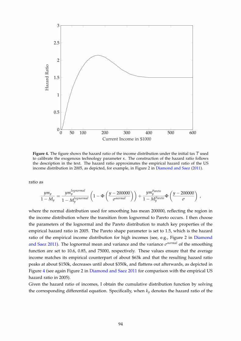
0 50 100 200 300 400 500 6000

0.5

1

1.5

2

2.5

3

Current Income in $1000

Haz

ard

Rat

io

Figure 4. The figure shows the hazard ratio of the income distribution under the initial tax T usedto calibrate the exogenous technology parameter κ. The construction of the hazard ratio followsthe description in the text. The hazard ratio approximates the empirical hazard ratio of the USincome distribution in 2005, as depicted, for example, in Figure 2 in Diamond and Saez (2011).

ratio as

ymy

1−My=

ymlognormaly

1−Mlognormaly

(1−Φ

(y− 200000

σnormal

))+

ymParetoy

1−MParetoy

Φ(

y− 200000σ

),

where the normal distribution used for smoothing has mean 200000, reflecting the region inthe income distribution where the transition from lognormal to Pareto occurs. I then choosethe parameters of the lognormal and the Pareto distribution to match key properties of theempirical hazard ratio in 2005. The Pareto shape parameter is set to 1.5, which is the hazardratio of the empirical income distribution for high incomes (see, e.g., Figure 2 in Diamondand Saez 2011). The lognormal mean and variance and the variance σnormal of the smoothingfunction are set to 10.6, 0.85, and 75000, respectively. These values ensure that the averageincome matches its empirical counterpart of about $63k and that the resulting hazard ratiopeaks at about $150k, decreases until about $350k, and flattens out afterwards, as depicted inFigure 4 (see again Figure 2 in Diamond and Saez 2011 for comparison with the empirical UShazard ratio in 2005).Given the hazard ratio of incomes, I obtain the cumulative distribution function by solvingthe corresponding differential equation. Specifically, when ky denotes the hazard ratio of the

94

income distribution, the cumulative distribution function solves

dMy

dy=

ky

y−

ky

yMy .

Finally, the density function of incomes is obtained as the numerical derivative of M.Since the distribution of types on the type space is uniform, the cumulative distribution func-tion of incomes M returns for each income the type who earns this income under the initialtax T. Hence, the income function y : θ 7→ yθ is given by the inverse of M.Given yθ , it is straightforward to compute κθ from workers’ first-order condition and the con-dition that wages equal marginal products of labor in aggregate production. First, multiplyingthe first-order condition (2) by lθ and solving for it yields

lθ =(

R′T(yθ)yθ

) e1+e ,

where I used that the disutility of labor is iso elastic in the quantitative analysis. With theestimate of T described in the main text, the previous equation allows to compute labor inputsunder T.For the second step, start from equations (13) and (42), copied here for convenience:

wθ(l, φ) = (κθφθ)σ−1

σ (lθhθ)− 1

σ F(l, φ)1σ

φ∗θ = C1δ (κθhθ lθ)

σ−1(δ−1)σ+1

[∫ θ

θ(κθhθ lθ)

(σ−1)δ(δ−1)σ+1 dθ

]− 1δ

.

The total amount of R&D resources C is not identified separately from κ, so I normalize it tosatisfy

C =∫ θ

θ(κθhθ lθ)

(σ−1)δ(δ−1)σ+1 dθ .

Using this normalization in the above equation for φ∗θ , plugging the equation into the expres-sion for the wage wθ , multiplying by lθ , and solving for κθ yields:

κθ = y1

1+γCES+ρCES

θ l−1θ F

γCES

1+γCES+ρCES .

With F =∫ θ

θ yθmy dy by Euler’s theorem, this allows to compute κ.Finally, the optimal tax formulae in Proposition 5 and Lemma 10 require the inverse hazardratio of the exogenous parameters β and β, respectively. In principle, β and β could be com-puted from κ and from the equilibrium technology under initial taxes via their definitions.Then, their pdf and cdf, and finally their hazard ratios could be computed. Here, to avoidunnecessary rounds of approximations, I choose a more direct way and compute the inversehazard ratios of β and β directly from the hazard ratio of the income distribution, using equa-tions (83) and (85). This ensures that the two hazard ratios inherit their shape directly from theshape of the initial hazard ratio of incomes (which is calibrated to match its empirical counter-part), without numerical differentiation or integration steps and the associated approximationerrors in between.

95