Redistributive Colonialism:

The Long Term Legacy of International

Conflict in India

May 16, 2014

Abstract

The growth of European colonial empires occurred during a period of

intense international conflict, the consequences of which are poorly under-

stood. This paper examines how the international position of colonial states

altered the distribution of wealth within indigenous societies. It proposes

that colonial administrators only transferred power to precolonial elites if

they were secure militarily and financially—while the local elite could pro-

vide colonizers a cheap and experienced group of administrators, they were

also its most threatening military rivals and richest taxpayers. This theory is

tested using data on the wealth of Indian caste groups. In areas annexed at

times of European war, precolonial elites are poorer than other groups, while

in other areas they remain richer. These results appear to not stem from pre-

existing differences between the two types of regions. The results highlight

the variable impact of colonialism within societies, and the strategic nature

of colonial policy choices.

Key words: colonialism, caste, state

2

1 Introduction

Numerous studies have shown that variation in colonial institutions can explain varia-

tion in contemporary economic and social outcomes (Acemoglu, Johnson and Robinson

2001; 2002; Mahoney 2010; Lee and Schultz 2012; Banerjee and Iyer 2005; Nunn 2009:

Iyer 2007). However, in their focus on the effect of long-term institutional factors, these

accounts have neglected the strategic rivalries and calculations into which colonial con-

quest was embedded. In particular, we have little understanding of whether European

political events and decisions, such as the persistent wars that plagued early-modern

Europe, altered colonial policy.

Similarly, the existing literature has focused on the institutional effects of colonialism,

rather than its distributional effects. Even within regions and nations, some social groups

may benefit from colonial policies, while others will be hurt by them, and these differences

may persist long after the official favoritism or distrust that gave rise to them has faded

away. However, we have little explanation for why colonial rule in some places reinforced

the social position of precolonial elites, while in others it weakened or replaced them.

This is not to say that these distributional effects are unstudied: Case studies pro-

vide strong evidence of colonial favoritism toward specific groups: The Belgians favored

Tutsis over Hutus in Rwanda, the British favored Tamils over Sinhalese in Sri Lanka,

the Spanish favored Tlaxcalans over Mexica in Mexico. Such favoritism is often thought

of as significant as a cause of later ethnic conflicts or social inequalities (Horowitz 1985).

However, such single-country accounts leave open many questions, including three po-

tentially important ones: 1) Why the process of colonialism systematically favored some

groups over others, 2) whether or not such favoritism actually altered existing patterns

of stratification, and 3) whether these effects have persisted to the present day.

This paper will show that relations between colonial administrators and their Indian

elites varied based the diplomatic situation in Europe. In European wartime, colonial

administrators felt insecure militarily, and tended to view the precolonial elite (the most

obvious leaders of a revolt) with suspicion. Similarly, in wartime the fiscal pressure

on the colonial state was much greater, increasing its incentive to expropriate elite

wealth. In European peacetime, the military and fiscal pressure on the colonial state

was less intense, and the colonial state found it more convenient to leave existing elites

in place, borrowing their personnel and (in indirectly ruled areas) their institutions.

Incorporation into colonial institutions in turn allowed these elite groups to maintain

high levels of socio-economic status. Since annexation represented a critical juncture

for the formation of local institutions and the selection of local elites, the effects of

conditions at this period often had effects that long outlasted the period of annexation

itself.

In estimating the effect of European war at the time of annexation, an obvious

potential concern is that assignment to treatment may be influenced by some attribute

of the units themselves, with colonial powers varying the type of territory they annex

based on geopolitical factors. There are theoretical reasons for thinking that biased

assignment is not a major problem in the Indian case: The dates of European wars were

decided in Europe rather than in India and annexation decisions tended to be highly

responsive to local political events. This is supported by the available data, since both

annexation and military conflict in India are uncorrelated with European conflict. There

is also strong support for the contention that areas annexed in European wartime and

European peacetime were similar in their social characteristics, since areas annexed at

times of European war appear very similar on geographical and social observables to

areas annexed at other times.

India, where there was considerable indigenous social stratification, and where the

colonial conquest was contemporaneous with a long series of on-and-off wars between

Britain and France, is an obvious place to test this theory. The question of cross-group

redistribution is particularly urgent in contemporary India, where intergroup economic

2

inequalities are very marked (today, 44% of modern variation in wealth can be explained

by caste.) In particular, there is substantial variation in the economic position of pre-

colonial landed groups. The fact that landed castes do better economically than other

Indians is not particularly surprising, given the sizable head start that they had over

most other social groups. What is surprising is that there is sizable variation in this

economic advantage. For example, while precolonial landed groups have an average

household wealth .64 standard deviations higher than non-landed groups in Bihar, they

are slightly poorer than non-landed groups in the neighboring state of West Bengal.

This variance has obvious direct relevance for the lives of millions of Indians, who find

themselves richer or poorer than their neighbors. It has an even greater indirect rel-

evance for the politics and political economy of India, since many students of Indian

politics, notably Srinivas (1966), and the contributors to Frankel and Rao (1989), have

traced variation in the political performance of Indian states to the social position of

landed caste groups.

The quantitative results show that while colonial-era wars have little impact on the

wealth of non-landed groups, they dramatically affect the wealth of landed ones. The

redistributive effects of colonialism appear to have been minimal in areas where there

was no European war at the time of annexation, since in these areas, landholding groups

perform better economically than non-landholding groups. In areas annexed in wartime,

this advantage is reversed, with non-landed groups being relatively wealthier than non-

landed ones. While wars in India during annexation have similar effects on landed elites

to war in Europe, international conflict is an important predictor of local distributional

patterns independent of local conflicts, whose intensity they tended to enhance. The

differing fates of landholding groups are unrelated to the land tenure institutions chosen

by the British, the party composition and fiscal situation of British governments, the date

of annexation, and subsequent changes in caste identity. A more tightly focused cases

study of the Indian state of Oudh shows that these dynamics were already apparent in

3

the colonial era, and provides evidence for the operation of a specific policy mechanism,

land confiscation for non-payment of taxes.

These results expand on existing work that emphasizes the importance of colonialism

in determining levels of social inequality (Engerman and Sokoloff 1998). However, while

such work examines the overall level of inequality in societies, this paper examines

whether the social inequalities introduced by colonialism reinforced or subverted existing

patterns. It also provides a counterpoint to several ideas about colonial policy with

the existing literature, notably that colonial powers tended to support weaker groups

against stronger ones (“divide and rule”) or supported groups with whom they identified

culturally (such as India’s “martial races”[Streets, 2004]) by showing that colonial policy

changed sharply over time, and was influenced as much by broader world events as by

characteristics of Indian groups.

Section Two will distinguish redistributive and non-redistributive varieties of colo-

nialism, and develop a theoretical framework for explaining their causes. Section Three

will describe why annexation in European wartime affected perceived colonial levels of

threat, and discuss how this effect deviates from an ideal experiment. Section Four will

describe the data used to measure colonial incentives and contemporary socio-economic

outcomes. Section Five will examine whether the effects of this variation persisted over

the two centuries since the British conquest, while Section Six will discuss an example

of how policies at annexation affected the landed castes in two parts of a single state,

Oudh. Section Seven will conclude with a discussion of how the distribution of wealth

that occurred during the colonial period has affected the course of Indian politics.

Due to space limitations, a large portion of the empirical analysis is described in

an online appendix. Section One provides additional tables, Section Two provides

additional historical context on British policy in India, Section Three discusses three

additional implications of the theory, Section Four consider factors that might create

pre-treatment differences between the war and peacetime-annexed samples, and Section

4

Five examines a wide variety of alternative hypotheses.

2 Colonial Favoritism

2.1 The Precolonial Distribution

Outside of the settler colonies, the administrators of the European empires were forced to

rule large existing populations.1 These populations often had developed fairly complex

systems of social stratification and hierarchy,2 which sometimes, though not always, were

aligned with ascriptive social categories.3 While the exact nature of this stratification

varied from place to place, one can identify a basic distinction between those groups that

controlled land and those that did not. In a pre-modern society, the control of land,

the principal source of economic production and government revenue, was inextricably

associated with the exercise of political authority. Landholding groups such as the

medieval European aristocracy, or the jagirdirs and zamindars of the Mughal Empire,

1This paper concerns the distributional consequences of colonialism among indigenous

populations, and why certain groups benefited from colonialism more than others. It thus

cannot explain conditions in areas where there was no precolonial population, or where

the precolonial population was quickly reduced to insignificance by war and disease, such

as in the settler colonies of the temperate zones, and some plantation colonies in the

tropics.2The theory here implicitly assumes that within the precolonial population we can

identify some social groups as being more powerful than others. In many societies,

particularly those comprised of hunter gatherers, such internal differentiation did not

exist (Ertan and Putterman 2007; Hariri 2012) and in these societies it is impossible to

examine the redistributive effects of colonialism.3See Author 2013b for a more detailed discussion of the relationship between ascrip-

tive ties and political hierarchy in pre-modern societies.

5

tended to dominate both revenue collection and the military, sometimes in opposition

to the states they were pledged to serve.

Pre-modern societies also possessed a number of other social groups, not all of them

poor. These included ordinary cultivators, who supported the landowning class with

their taxes, and enabled the landholding class a degree of specialization in political

and military action. It also included several groups with weaker ties to the land, such

as village craftsmen, long distance traders, and religious or clerical specialists. While

members of these groups could be quite wealthy, and could sometimes participate in

politics, their power at a local level was usually much weaker than that of the landholding

elite. In India specifically, the fragmentary historical data indicate that landed castes had

a very marked socio-economic advantage in the precolonial period. Traveler’s accounts

of India frequently contrast the miserable economic position of village laborers and

craftsmen to those of farmers, and that of tenant cultivators to those of more secure

agricultural proprietors (Chandra 1982; Fukazawa (1982). The concentration of political

power within landed groups became even more marked after the collapse of Mughal

power, as the anarchic conditions prevailing in many parts of South Asia in the 18th

century enabled local zamindars to assert their independence, at times acquiring sizable

military forces (Kolff 1990), and in the cases of the Rohillas, Marathas, Jats and Sikhs,

large empires.

Colonial administrators could potentially distribute resources among these groups in

a variety of patterns. If colonial rule favored the landholders, the power structure of

society would not change fundamentally, though the aggregate level of inequality within

the society would become larger. More drastically, a colonial government could ignore

the landholding groups and create a new bureaucracy with native or imported personnel,

potentially upending existing social orderings. In the next few pages, we will see how

colonial officials choose among these strategies.

6

2.2 Censorship of the Data

One obvious argument about the relationships between colonial strategy and local elites

is that the weaker the colonial power (whether fiscally or militarily) the more likely it is

too ally with local elites A militarily weak colonial state, this argument runs, would need

the most powerful allies it could get, and would thus prefer to accommodate existing

powerholders, and might have difficulty displacing them even if it wished to.

However, this causal logic is unlikely to apply to actual colonial states. While situ-

ations where Europeans were very weak in relation to indigenous powers have occurred

throughout world history, they are likely to be censored out of most datasets on colo-

nialism, since in these conditions the European power would be unable to establish for-

mal rule. Such an alliance between European weakness and indigenous strength would

resemble instead an ordinary alliance of two powers, or a loose protectorate, rather

than colonialism as we understand it. In the South Asian context, the local elites of

Afghanistan maintained a strong military position relative to the British, and were thus

able to avoid colonial rule entirely, and thus avoid being included in a sample of colo-

nial landed groups. Such arrangements were particularly common in the Early Modern

period, when European military superiority was less assured than it later became. The

British French and Dutch, for instance, all cultivated friendly and deferential relations

with the major Indian powers until the mid-eighteenth century. Any discussion of “colo-

nial strategy” or “colonial annexation” thus carries an implied scope condition: That

the European power possess a minimal military superiority over the local elite.

2.3 The Military Goals of the Colonial State

While colonial states differed in the degree to which they were motivated by economic,

altruistic, or strategic goals, all of these objectives required the perpetuation of colonial

rule, and colonial regimes thus sought to secure themselves against both external and

7

internal military threats. In retrospect, their triumph over these threats seems preor-

dained: Colonial militaries were usually superior in both technology and organization

to their indigenous opponents, and these advantages often gained them victories against

vast numerical odds. As we have seen, militarily weak European states were incapable of

creating colonies in the first place. However, victory was not always cheap or automatic.

Even if indigenous states could be subdued quickly, guerrilla struggles could drag on for

years, as in Libya, Burma, and the Philippines, making the colony hardly worth the con-

quest. Even after all resistance had been subdued, the small numbers of the colonizers

made revolt a terrifying possibility, as the British learned to their cost in India in 1857.

To foreclose such possibilities, colonial powers emulated modern authoritarian regimes

both in conducting brutal reprisals against rebels and in creating elaborate systems of

“coup proofing” within their militaries.

To conquer a territory, colonial powers necessarily had to either intimidate or defeat

the precolonial elite, who controlled the coercive capacity of their polities, and thus

the capacity of these polities for resistance. In the initial stage of colonial institution

building, Europeans thus tended to be at risk militarily from members of this group, and

to perceive this group as threatening. Even after the conquest was completed, members

of such groups were the most likely leaders of a revolt against the colonial state, both

because of their inherited military skill and social contacts and because they tended to

view themselves, not unreasonably, as the natural rulers if Europeans were removed.

This threat, while always present, became more urgent due to external interference.

Colonial states were not only fighting the local inhabitants, but each other, and the rival-

ries among European powers assumed a very high priority in colonial security planning.

A particular paranoia of many colonial rulers was that their foreign and internal ene-

mies would combine, with native opponents joining the invading army, or being provided

with modern arms and training to revolt on their own (Yapp 1987). This fear was by

no means unreasonable: many of the most successful indigenous political entrepreneurs

8

of the colonial era, such as the Emperor Menelik of Ethiopia or Haider Ali of Mysore,

were assiduous in playing the colonial powers off against each other. All but the most

torpid pre-modern states were enthusiastic consumers of European weapons and Euro-

pean military advisors. Nor were such strategies always unsuccessful: Menelik used his

French rifles to decisively defeat the Italians and maintain his country’s independence,

while French officers were at the head of the Mysore and Maratha armies that posed the

last serious challenge to British hegemony in India. 4

What made the prospect of external aid particularly credible was that the during

the period of colonial expansion endemic military conflict in Europe gave rival powers

strong incentives to aid their enemy’s enemies in Asia and Africa. From 1756 to 1763,

1778 to 1783, 1793 to 1802, 1803 to 1815 and 1854 to 1856 Britain was at war with

France or Russia, meaning that these powers, could and did, aid indigenous elites. In

wartime, the prospect of external aid narrowed the margin of military superiority which

the colonial power possessed over the indigenous elite, at times to dangerous levels

2.4 The Fiscal Goals of the Colonial State

Even if local elites remained perfectly quiescent, European Wars were stressful periods

for colonial administrators, since they increased the fiscal demands on the colonial state.

Even without allies, European enemies could attack a colony directly, with the task of de-

fense being borne by the local budget. Similarly, the government in the metropole might

demand that a colony finance an expedition against the colonies of its rival, as when the

Indian government conquered Mauritius on Britain’s behalf in 1810. Finally, the central

4In addition to external aid, numerous other factors might influence the relative

military capabilities of the colonizing power and the indigenous elite, including the time

of colonization, the size of the European state and the institutional development of the

indigenous polity.

9

government could make or indirect demands for funds, as the British government made

of the East India Company during its 18th century wars.

The result of this increase in fiscal pressure was that colonial official needed to collect

more revenue. This put pressure on indigenous elites in two ways. Firstly, as owners

of the most important and most visible economic asset, land, any increase in revenue

demands would fall disproportionately on them. Secondly, indigenous elites were often

beneficiaries of arrangements by which they collected taxes on behalf of the state, re-

taining a portion of the revenue for their trouble. The jagirdirs and zamindars of 18th

century India, for instance, like the chiefs of colonial Africa, derived much of their status

from this tax farming role, which had helped reconcile many of them to colonial rule.

However, in circumstances of fiscal stringency such arrangements were likely to be per-

ceived as inefficient luxuries, which colonial officials would avoid in favor of more direct

taxation.

2.5 The Administrative Goals of the Colonial State

The fiscal potential of incumbent groups, and the high level of military threat they

posed, by was counterbalanced by another factor—that it was cheap and convenient to

work through them. As the traditional administrators of the country, they had access

a set of social networks and institutions that enabled them extract revenue from and

administer justice to politically weaker groups. While the colonial regime could replace

them with new men, either outsiders or members of non-landholding groups, such an

effort would involve the creation of an expensive set of new institutions. In addition, the

new administrators were likely to be inexperienced in their jobs and would certainly lack

the veneer of legitimacy that had eased the extraction of their predecessors. In early

19th century Uttar Pradesh, for instance, the British found it difficult to find new buyers

for the estates of rebellious or bankrupt landlords, since potential buyers knew it would

be difficult, and perhaps physically dangerous, to collect rents and taxes as outsiders in

10

the face of opposition from the relatives and clients of their predecessors (Metcalf 1979).

When buyers could be found, they often offered little money to the government, since

they were aware of the problems they would face in exercising authority.

Such efforts to replace indigenous elites wholesale thus tended to be both expensive

and violent. In upper Burma, for example, the British found themselves unable to trust

the lowland Burmans, against whom they were waging a large and atrocity-filled coun-

terinsurgency campaign. The new regime thus ignored both the Burmese upper class and

its institutions, instead importing bureaucrats and policemen from India, supplementing

them with members of previously marginalized minority groups (Furnivall 1948). The

result was a colonial state that had chronic difficulty both collecting taxes and main-

taining law and order, problems that became evident in its swift collapses during the

Saya San rebellion and the Second World War.

There were several means by which colonial regimes were able to avoid this kind

of disruption, and incorporate existing elites into their administrative structure. The

easiest to implement was to simply leave the precolonial institutions as they were, and

allow them to continue their existing practices in return for their acknowledgement of

European hegemony. This pattern, usually referred to as indirect rule, was very com-

mon within European empires, though there was considerable variation in the amount of

autonomy allowed, the degree to which these institutions actually were reflective of tra-

ditional ones, and the political level at which indigenous rulers were allowed to operate.

In French West Africa, for instance, traditional chiefs were little more than low-level

bureaucrats, frequently unrelated to the traditional ruling lineages. British India, by

contrast, included many princely states of considerable size, often ruled by the descen-

dants of the eighteenth century rulers. While even the largest princely states retained

nothing resembling independence, their existence enabled rulers to retain a measure of

authority and influence, and the ability to offer jobs to their relatives and coethnics.

Even when the colonial power chose to administer an area directly, it could take

11

steps to ensure that the existing elite retained a position of political importance. It

could, for instance, hire members of the former ruling groups for positions within its

bureaucracy, and provide them with educational opportunities. Even if it did not have a

conscious policy on hiring, its choice of the language of administration and the cultural

practices of the government could influence which groups sought employment there. In

Northern India, for instance, the maintenance of Persian as the language of the courts

until the 1870s favored official employment of Muslims, while its replacement by English

disadvantaged them. Even when the government included few locals, the colonial regime,

could favor or disfavor a group through the expropriation of property, a process that

occurred all too frequently during the colonial period. Those traditional elites that

maintained their land were in an excellent position to maintain some of their existing

political position, often through the capture of local administrative and judicial posts.

2.6 Critical Junctures

Colonialism was a process that lasted at least several decades, and at most several

centuries. During this time, colonial states were free, at least in theory, to pursue a

wide variety of policies. However, the choices made in the period immediately after the

conquest exercised a disproportionate influence on what options were available, since

reversing these choices was often difficult or impossible. Most importantly, authorities

at the time of conquest faced a choice as to which elements of the precolonial elite

and institutional arrangements to retain. If they choose to destroy these institutions,

future generations of officials would find it difficult or impossible to reconstruct them

from scratch (Furnivall 1948). If they choose to retain them, later officials often found

themselves tangled in a web of commitments that made dismissing local officials difficult.

Even when colonial officials choose to construct their local elites from scratch, the

choices made at the time of conquest tended to narrow their options later. At the time

of conquest, European educational and political institutions were a novelty, and were

12

not associated with any particular social group. After the first generation, however, the

groups that had gained access in the early years would have a good chance of keeping that

position in later years, due to their familiarity with and connections within the existing

system. Changes to the institutional structure as a whole would also be frustrated by

the interest group resistance and institutional stasis described in the literature on critical

junctures, effectively freezing in place the patterns of favoritism that were seen at the

time of the conquest. This is not to say that colonial policy would not evolve as the

security situation changed: In India for instance, favoritism toward the martial races in

military recruitment emerged only after 1857. However, we should expect such policy

changes to be less effective in areas where they reversed earlier policies and challenged

established interest groups than where they favored these groups.

2.7 Predictions

This section examined three major factors in the internal calculations of colonial bureau-

crats: Suspicion of revolt and military threat, desire to raise revenue and the inconve-

nience and expense of replacing indigenous landholding elites wholesale. Military threat

and fiscal necessity would tend to encourage discrimination against indigenous elites in

favor of outsiders or less powerful groups, while administrative convenience would tend

to encourage favoritism toward of the existing elite. While the influence of all these

factors should change over time, they should be disproportionately influenced by cir-

cumstances at the time of annexation. In particular, the existence of a war in Europe

at annexation should threaten the colonial regime and increase its need for money, and

should thus be a strong negative predictor of the level of the regime’s willingness to

incorporate existing elites. Elite incorporation, in turn, should be associated with high

levels of socio-economic status, since political power, western education and control over

land all can easily be translated into economic resources. The hypothesized empirical

relationship can be summarized as:

13

Wartime Annexation → Colonial Military Threat → Low Elite Incorporation → Low

Elite Socio-Economic Status

Which can be restated as:

H1: In areas annexed at times when the colonial power is at war elsewhere,

the pre-colonial elite will tend to have lower socio-economic status relative to

other groups than in areas than in areas where colonial institutions annexed

when the colonial power was as peace.

3 European Conflict and Military Threat

3.1 European Wars and Indian Policy

The idea that war and peace in Europe affected military strategy and fiscal policy in

South Asia is echoed in the historical literature. In particular, European wars put

increased demands on the colonial military. In the 1750s, this took the form of a regular

war in South India, where the French had a sizable army and a territorial presence. After

this period however, the threat outsiders posed to the British was less from the direct

use of troops as from their potential influence over Indian powers. In Hyderabad, Bengal

and Carnatic, there were recognized pro-French parties at court, and at Hyderabad in

particular the French succeeded in using their control of the western-trained army to

virtually dictate state policy. Indian rulers were well aware that the French presence gave

them an outside option in the weapons trade—the first Anglo-Mysore War was prompted

by Mysore’s anger at the British capture of their former source at the French fort at

Mahe 1779, itself a result of France’s involvement in the American Revolution. Such

contacts continued during the revolutionary wars, during which a large French military

mission was sent to Mysore in 1798. European soldiers of fortune also contributed to

the military efficiency of the Maratha and Sikh armies (Bidwell 1971).

14

These international connections caused considerable unease in the English camp, and

it is notable how rulers who intrigued with the French were much more severely dealt

with than those who did not. Tipu Sultan of Mysore, in particular, became something

of an Anglo-Indian hate figure, with his alliance with the French taken as evidence as a

global conspiracy against British liberties (Forrest 1970). After his defeat, Tipu’s Muslim

dynasty was deposed and replaced by a Hindu one. A similar process occurred in Bengal

in 1760, where the British discovered that the Nawab, Mir Jafar was attempting to form

a military alliance with the Dutch East India Company. This led to the deposition

of the Nawab, the annexation of the coastal portions of his territory, and the further

involvement of the Company in Bengali politics. Fear of French and Dutch involvement

was also a major factor in the First Anglo-Maratha War (1775-1778) and the peace

treaty that ended the war granted sizable territorial concessions to the Marathas in

return for a promise not to have dealings with any other foreign power. These examples

could be multiplied ad nauseam, even after 1815, where the Russian threat was often

perceived as more threatening than the French one.

This concern is reflected in correspondence between colonial officials, who frequently

comment on and debate the probable consequences of war and peace in Europe. To

take one example, a sizable crisis within the governor general’s council was caused by

the news, in the spring of 1778, that France was planning to enter the American Revo-

lutionary war, which lead Phillip Francis to call for a rethink of company policy.

“I would wish that the board consider whether this unfortunate event inAmerica ought not to have a general influence upon our measures here...andwhether policy and prudence do not plainly indicate to us that, while thenation is so deeply engaged and pressed on one side, with everything toapprehend from the designs of France and Spain on the other, that we shouldstand on the defence.”5

5 Forrest, George, and Warren Hastings.Selections From the Letters, Despatches and

Other State Papers Preserved In the Foreign Department of the Government of India,

15

The poorer security situation during European wars was reflected in the Company’s

fiscal situation. Focusing only on years in which annexations took place, the companys

military expenditure averaged 57.2% of expenditure in European war years and 46.2%

in European peace years. 6 Combined with slightly higher civilian expenditure (often

on war related expenses like ships, forts and debt service) the companys expenditure

increased by 24% in European wartime.

3.2 European Wars and Annexation Policy

While military conflicts in Europe might well affect the colonial state’s military and fiscal

strain, areas annexed in wartime might also be different from each other in a number

of ways that might be correlated with their contemporary economic position. However,

the historical evidence about particular annexation supports the idea that the timing

of conquest in India depended largely on local political factors, such as the deaths of

Indian rulers and British military success in India. If annexation processes were similar

in wartime and peacetime, it would provide strong evidence that the annexed areas were

similar.

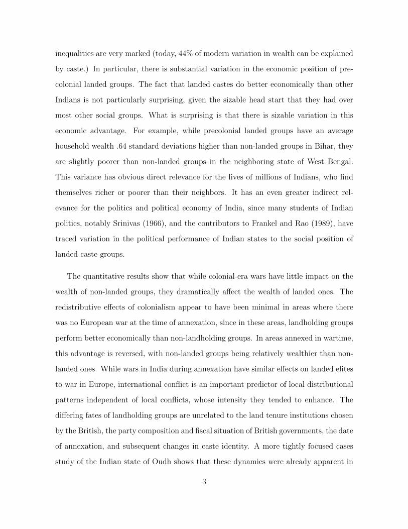
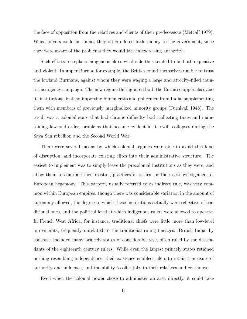
One of the strongest pieces of evidence for this view is that annexation is uncorrelated

with European War. Of the 251 1991 districts of India that were directly ruled, 78

(30.3%) were annexed during years of Europeans war, which covered 32.7% of the years

during this period.7 Figure One shows this pattern graphically: Annexation is just as

prevalent in wartime as in peacetime.

Even more interestingly, military conflict in India is uncorrelated to military conflict

1772-1785. Vol. II. Calcutta: Government Printing, 1890. P.632.6Accounts respecting the annual revenues and disbursements, trade and sales of the

East India Company. London: Various Years.7Of the 110 years from 1756 to 1865 (when the last part of British India was annexed)

36 were periods of European war.

16

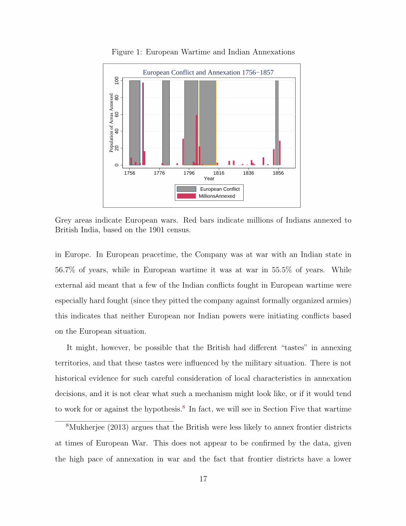
Figure 1: European Wartime and Indian Annexations

020

4060

8010

0P

opul

atio

n of

Are

as A

nnex

ed

1756 1776 1796 1816 1836 1856Year

European ConflictMillionsAnnexed

European Conflict and Annexation 1756−1857

Grey areas indicate European wars. Red bars indicate millions of Indians annexed toBritish India, based on the 1901 census.

in Europe. In European peacetime, the Company was at war with an Indian state in

56.7% of years, while in European wartime it was at war in 55.5% of years. While

external aid meant that a few of the Indian conflicts fought in European wartime were

especially hard fought (since they pitted the company against formally organized armies)

this indicates that neither European nor Indian powers were initiating conflicts based

on the European situation.

It might, however, be possible that the British had different “tastes” in annexing

territories, and that these tastes were influenced by the military situation. There is not

historical evidence for such careful consideration of local characteristics in annexation

decisions, and it is not clear what such a mechanism might look like, or if it would tend

to work for or against the hypothesis.8 In fact, we will see in Section Five that wartime

8Mukherjee (2013) argues that the British were less likely to annex frontier districts

at times of European War. This does not appear to be confirmed by the data, given

the high pace of annexation in war and the fact that frontier districts have a lower

17

and peacetime-annexed areas are similar on observables.

To further address the possibility that areas annexed in wartime are systematically

different than those annexed in peacetime, the exogeneity of European wars to annex-

ation time will be tested in Section Five and Section A-4, both by comparing the two

types of areas on precolonial conditions and on variables that might affect annexation

policy. Some of the important controls that have little effect of group wealth are the

year of annexation, the political party in power in England, the fiscal situation of the

East India Company, and the level of military conflict within India.

3.3 Departures from the Ideal Experiment

Even if European political events are exogenous to annexation policy in India, the as-

signment of Indian districts to wartime or peacetime annexation differs in several key

respects from random assignment. Firstly, the time of annexation tends to be lumpily

distributed in space, as the British annexed large tracts of territory at a time. The entire

modern state of Bihar, for instance, was annexed at once in 1765. In this situation, not

only will estimates of the effect of wartime annexation have inflated standards errors, but

the coefficients may be biased, since regions might have different internal distributions

of wealth. To address this problem, all reported results cluster their standard errors at

the district level, to account for the non-independence of observations within districts.

Some models also include fixed effects for precolonial states, to control for differences in

wealth across regions.

Secondly, even within regions, districts annexed at times of European war might

differ from those annexed at other times, perhaps because European wars are correlated

with some underlying spatial difference. This is a particular problem since European

probability of annexation at all times. Even if this suggestion is correct, however, it

would not necessarily follow that areas annexed in European wartime are distinct in

their social characteristics from those annexed in peacetime.

18

wars were more numerous in the earlier part of the period of imperial expansion. To

address this concern, Section Five discusses a series of tests of whether the wartime-

annexed districts are identical to the peacetime-annexed districts in ways that we can

observe, such as their topography, demography, and precolonial politics. As we shall

see, after adjusting for regional clustering the treatment and non-treatment groups are

substantially identical on observables. In addition, Section A-4 includes an extensive

set of controls and robustness checks, designed to show that any difference between the

two groups is not driven by differences in their spatial characteristics, or in the date of

annexation.

Thirdly, the treated group, the landed castes, varies significantly in nature from

region to region. In some areas, such as the northern Hindi-speaking states, the landed

castes are generally “twice born,” with a high status within the Hindu caste hierarchy,

while in other states the landed elite is composed of slightly less prestigious upper

peasant groups. Similarly, in some areas, the landed castes take in a small portion

of the population, while in other areas they include a substantial plurality, including

many poor people.

In a large sample where treatment is exogenous, this problem will be unimportant,

since the cultural and economic differences among groups will tend to even out. However,

the efficiency of this model can be improved by controlling for these differences. The

major reported results include controls for the percentage of landed castes in the district

and the interaction of that variable with a dummy for landed castes. The reported

results are thus conditional on the local social position of groups.

19

4 Data

4.1 Time of Annexation

In this study, the year of annexation is measured at the level of the 1991 district of

India. This was chosen rather than the precolonial territory because many precolonial

polities had different parts of their territory annexed at different times.9 Jammu and

Kashmir, the hill states of Northeastern India, and the directly-ruled union territories

were excluded from the analysis.10 The main analysis will code annexation as occurring

in the year the East India Company formally acquired the right to collect taxes in a

district, coded based on Schwartzenburg and Bajpai (1978) and Dodwell (1922).

To account for the spatial lumpiness of the wartime annexation variable, the reported

models include fixed effects for precolonial states and have their standard errors clustered

at the level of the district. For this purpose, precolonial states are coded based on the

1756 status quo and given in Schwartzenburg and Bajpai (1978) and Dodwell (1922).

For this purpose, certain areas dominated by interrelated groups of small chieftains, such

as the Sikh confederacy in the Punjab, were coded as single polities. Altogether this

method divided India into 84 18th century states, of whom 36 had some portion of their

territory directly annexed.

4.2 The Landed Castes

Defining social groups in the Indian context is a complicated process, since groups are

often nested within the others, or part of cleavage dimensions that crosscut each other.

9Districts are also the level at which spatial assignment was made, since information

on location is not available below this level.10These areas were either not colonized by Britain, were developed in the 20th century,

or are border regions with long histories of civil conflict.

20

In this paper, I use the basic unit of the caste system, the jati.11 Jatis are of relatively

small size, and are often tightly specialized by occupation, making the sorting of jatis

into landholding classes relatively straightforward. Also, since caste as a dimension was

highly relevant to colonial policy makers, (Dirks 2002, Author. 2013a) we have reason

to expect that any British favoritism would be directed along caste group lines.

Only a few of these castes, however, have the traditional social prestige and connec-

tion with landed political power that defined the precolonial elite. I code these landed

castes based on the provincial volumes 1911 census, which listed the traditional occupa-

tions for groups as defined by the colonial authorities. I coded as landed castes whose

traditional occupation was listed as “landowning,” “military” or “dominant.”’ The re-

sults are robust to also including the much larger but poorer and lower status set of

castes whose occupation was given as “agriculture” or “cultivation” (Table A-9, Model

2).

4.3 The Dependent Variable

The dependent variable of interest in the modern era is the socio-economic status of

individuals. Socio-economic status is a broad concept, and includes not only wealth

but education, occupation and generalized level of social status. The main results will

concentrate on wealth, measured at the household level. Wealth was chosen because it

does not suffer from the substantial unobserved heterogeneity that we observe within

occupational categories and educational levels, and because it is less influenced than

education or literacy by changes in state policy over the past few decades.

The individual data was taken from the second round of the National Family Health

Survey, conducted in the cool season of 1998-1999 and made available in a recoded

11Jati is self-reported in the 1998 National Family Health survey. Individuals reported

thousands of spelling variants and local titles, which were recoded as the main caste.

21

version through Measure DHS (International Institute for Population Sciences 2000).12

Unlike the vast majority of Indian surveys, the NFHS records the actual caste of the

individuals, making it uniquely suitable for studying group-level redistribution. The

data was collected through a clustered design with the clusters representing either urban

neighborhoods or rural villages.

Within the NFHS data, wealth is measured as a factor score based on whether a

household possesses a set of household goods or improvements, such as radios, bicycles,

paved floors and kerosene stoves. This indirect approach to measuring wealth is common

in surveys in poor countries, given that many households hold large portions of their

wealth in assets that are not easy to value in cash. By construction, this measure has a

mean of zero and a standard deviation of one.

4.4 The Unit of Analysis

The quantity of interest for the theory is the difference in wealth between landed and

non-landed castes in different types of districts. The unit of observation is thus the

district-caste category, with two observations per district (one each for landed and non-

landed groups.)

There are a variety of alternative ways of organizing the analysis, none of which

affect the results substantively. These include confining the dataset landed castes and

estimating the effect of threat directly, taking the differences in category wealth for each

district as the quantity of interest, taking the district-jati as the unit of observation and

taking the household as the unit of observation (preserving the original structure of the

survey data). These alternative specifications are reported in Table A-9.

12This round of the NFHS was chosen because it is the most recent to include infor-

mation on the home district of respondents.

22

4.5 Estimating Equation

Since we are interested in the effect of Wartime Annexation on Landed Castes, the

independent variable of interest is the interaction of these two variables. The basic

model, estimated as Model One of Table Two, is thus:

Wealthcd = πLandedCastec + δWarAnnexd + ρWarAnnexd ∗LandedCastec + εjd (1)

With Wealthcd being the wealth of each caste category-district and ρ being the

coefficient of interest.

In all these models, the standard errors will be clustered at the district level, to ac-

count for the possible non-independence of observations of group wealth within districts.

5 Results

5.1 Balance

Were regions annexed are time of European war similar to regions annexed at times of

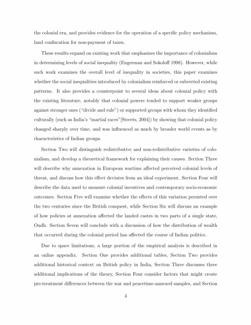
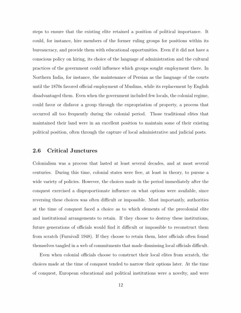
European peace? Figure Two shows the distribution of wartime-annexed districts rela-

tive to princely and peacetime-annexed districts. The princely states possess a distinct

spatial pattern, being concentrated in inland areas and in the west of the subcontinent.

The relative distribution of annexation dates relative to European war is less distinct.

On the one hand, the annexation of whole regions at the same time means that the

distribution of wartime annexation is spatially clustered. On the other hand, these

regional concentrations do not appear to be correlated with any of the superregional

distinctions within India well-known to scholars, such as the distinction between north

and south, and between zamindari and non-zamindari land tenure. Within states, the

divisions between annexation dates are fairly arbitrary. We should thus expect the dif-

ferences between the treated and non-treated samples to be minor after accounting for

23

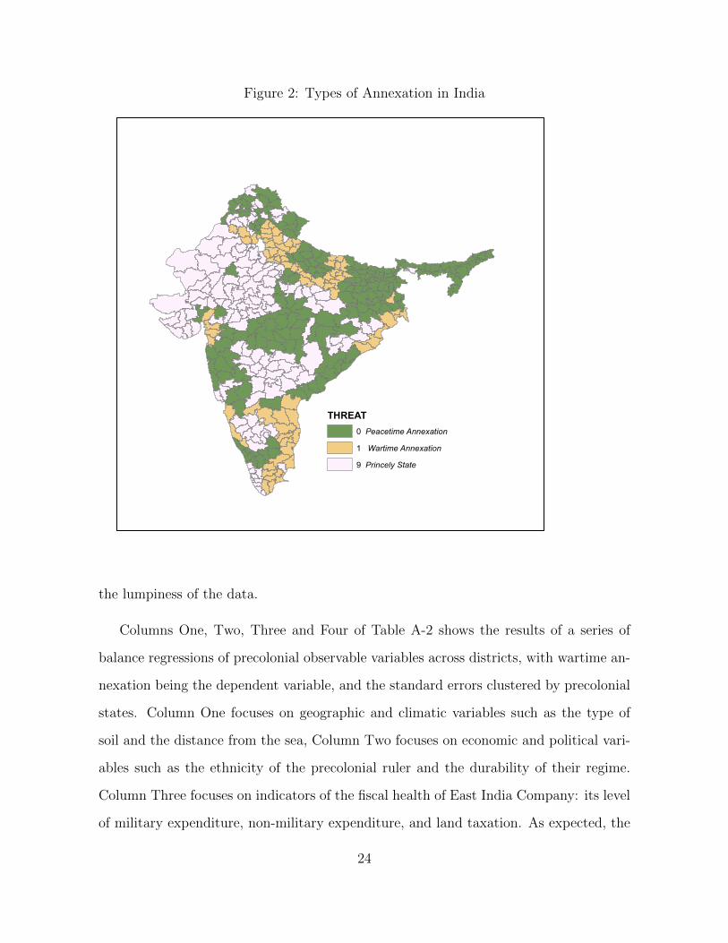
Figure 2: Types of Annexation in India

THREAT0 Peacetime Annexation1 Wartime Annexation9 Princely State

the lumpiness of the data.

Columns One, Two, Three and Four of Table A-2 shows the results of a series of

balance regressions of precolonial observable variables across districts, with wartime an-

nexation being the dependent variable, and the standard errors clustered by precolonial

states. Column One focuses on geographic and climatic variables such as the type of

soil and the distance from the sea, Column Two focuses on economic and political vari-

ables such as the ethnicity of the precolonial ruler and the durability of their regime.

Column Three focuses on indicators of the fiscal health of East India Company: its level

of military expenditure, non-military expenditure, and land taxation. As expected, the

24

level of military expenditure is higher in war annexed areas than elsewhere, while other

levels are similar. Column Four focuses on ex-post demographic variables such as the

percentage of Muslims and members of Scheduled castes and scheduled tribes in the

population. Wartime and peacetime-annexed areas do not appear to differ substantially

on any of these variables. The only statistically significant differences concern precolo-

nial changes in sovereignty (at the 10% level), and alluvial soils. Given the large number

of variables in the specifications, the statistical significance of these variables may well

not be causal. The online appendix shows that variation in these variables does not

appear to be driving the reported results. These results underline a basic aspect of the

research design: That areas annexed in European and wartime and European peacetime

were relatively similar to each other at the time of annexation.

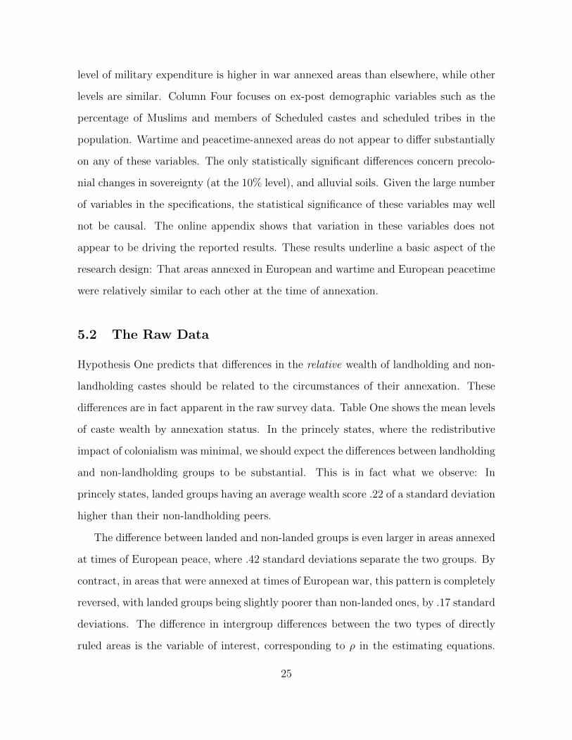
5.2 The Raw Data

Hypothesis One predicts that differences in the relative wealth of landholding and non-

landholding castes should be related to the circumstances of their annexation. These

differences are in fact apparent in the raw survey data. Table One shows the mean levels

of caste wealth by annexation status. In the princely states, where the redistributive

impact of colonialism was minimal, we should expect the differences between landholding

and non-landholding groups to be substantial. This is in fact what we observe: In

princely states, landed groups having an average wealth score .22 of a standard deviation

higher than their non-landholding peers.

The difference between landed and non-landed groups is even larger in areas annexed

at times of European peace, where .42 standard deviations separate the two groups. By

contract, in areas that were annexed at times of European war, this pattern is completely

reversed, with landed groups being slightly poorer than non-landed ones, by .17 standard

deviations. The difference in intergroup differences between the two types of directly

ruled areas is the variable of interest, corresponding to ρ in the estimating equations.

25

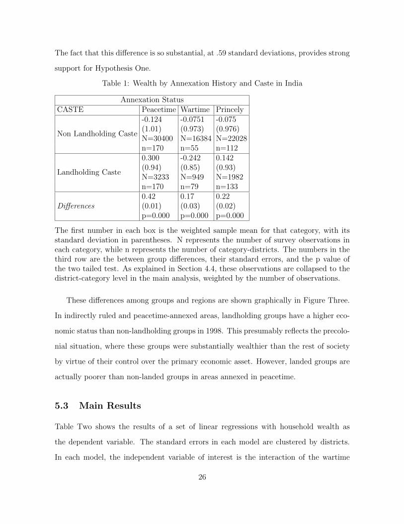
The fact that this difference is so substantial, at .59 standard deviations, provides strong

support for Hypothesis One.

Table 1: Wealth by Annexation History and Caste in India

Annexation StatusCASTE Peacetime Wartime Princely

Non Landholding Caste

-0.124 -0.0751 -0.075(1.01) (0.973) (0.976)N=30400 N=16384 N=22028n=170 n=55 n=112

Landholding Caste

0.300 -0.242 0.142(0.94) (0.85) (0.93)N=3233 N=949 N=1982n=170 n=79 n=133

Differences0.42 0.17 0.22(0.01) (0.03) (0.02)p=0.000 p=0.000 p=0.000

The first number in each box is the weighted sample mean for that category, with itsstandard deviation in parentheses. N represents the number of survey observations ineach category, while n represents the number of category-districts. The numbers in thethird row are the between group differences, their standard errors, and the p value ofthe two tailed test. As explained in Section 4.4, these observations are collapsed to thedistrict-category level in the main analysis, weighted by the number of observations.

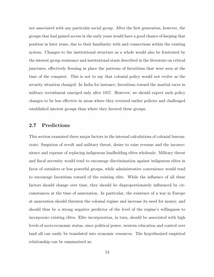
These differences among groups and regions are shown graphically in Figure Three.

In indirectly ruled and peacetime-annexed areas, landholding groups have a higher eco-

nomic status than non-landholding groups in 1998. This presumably reflects the precolo-

nial situation, where these groups were substantially wealthier than the rest of society

by virtue of their control over the primary economic asset. However, landed groups are

actually poorer than non-landed groups in areas annexed in peacetime.

5.3 Main Results

Table Two shows the results of a set of linear regressions with household wealth as

the dependent variable. The standard errors in each model are clustered by districts.

In each model, the independent variable of interest is the interaction of the wartime

26

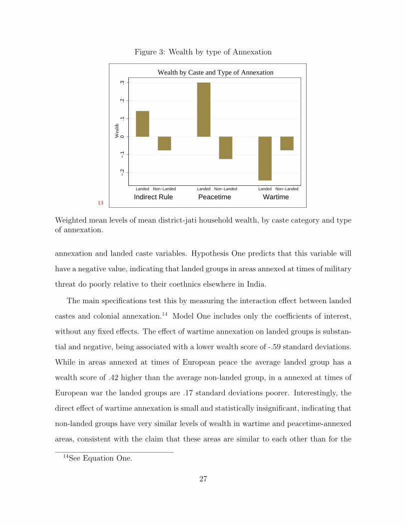
Figure 3: Wealth by type of Annexation

13

−.2

−.1

0.1

.2.3

Wea

lth

Indirect Rule Peacetime WartimeLanded Non−Landed Landed Non−Landed Landed Non−Landed

Wealth by Caste and Type of Annexation

Weighted mean levels of mean district-jati household wealth, by caste category and typeof annexation.

annexation and landed caste variables. Hypothesis One predicts that this variable will

have a negative value, indicating that landed groups in areas annexed at times of military

threat do poorly relative to their coethnics elsewhere in India.

The main specifications test this by measuring the interaction effect between landed

castes and colonial annexation.14 Model One includes only the coefficients of interest,

without any fixed effects. The effect of wartime annexation on landed groups is substan-

tial and negative, being associated with a lower wealth score of -.59 standard deviations.

While in areas annexed at times of European peace the average landed group has a

wealth score of .42 higher than the average non-landed group, in a annexed at times of

European war the landed groups are .17 standard deviations poorer. Interestingly, the

direct effect of wartime annexation is small and statistically insignificant, indicating that

non-landed groups have very similar levels of wealth in wartime and peacetime-annexed

areas, consistent with the claim that these areas are similar to each other than for the

14See Equation One.

27

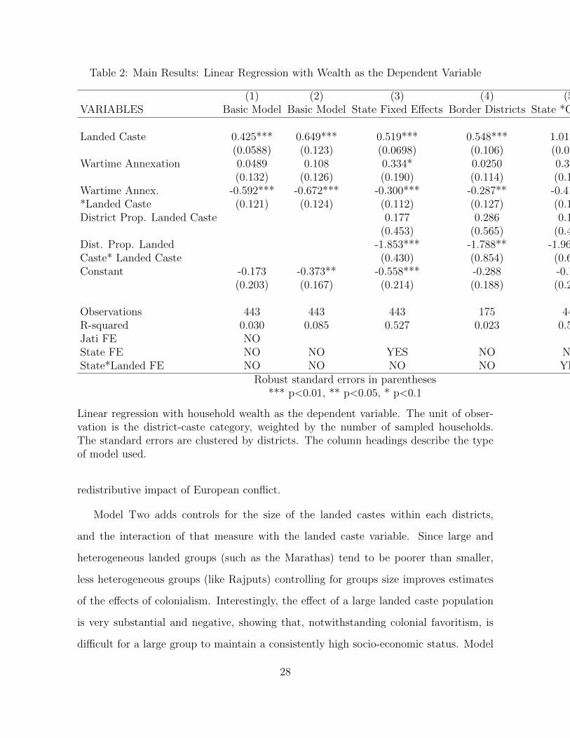
Table 2: Main Results: Linear Regression with Wealth as the Dependent Variable

(1) (2) (3) (4) (5)VARIABLES Basic Model Basic Model State Fixed Effects Border Districts State *Caste FE

Landed Caste 0.425*** 0.649*** 0.519*** 0.548*** 1.012***(0.0588) (0.123) (0.0698) (0.106) (0.0228)

Wartime Annexation 0.0489 0.108 0.334* 0.0250 0.335*(0.132) (0.126) (0.190) (0.114) (0.198)

Wartime Annex. -0.592*** -0.672*** -0.300*** -0.287** -0.415***Landed Caste (0.121) (0.124) (0.112) (0.127) (0.181)District Prop. Landed Caste 0.177 0.286 0.181

(0.453) (0.565) (0.499)Dist. Prop. Landed -1.853*** -1.788** -1.969***Caste* Landed Caste (0.430) (0.854) (0.684)Constant -0.173 -0.373** -0.558*** -0.288 -0.100

(0.203) (0.167) (0.214) (0.188) (0.241)

Observations 443 443 443 175 443R-squared 0.030 0.085 0.527 0.023 0.533Jati FE NOState FE NO NO YES NO NOState*Landed FE NO NO NO NO YES

Robust standard errors in parentheses*** p<0.01, ** p<0.05, * p<0.1

Linear regression with household wealth as the dependent variable. The unit of obser-vation is the district-caste category, weighted by the number of sampled households.The standard errors are clustered by districts. The column headings describe the typeof model used.

redistributive impact of European conflict.

Model Two adds controls for the size of the landed castes within each districts,

and the interaction of that measure with the landed caste variable. Since large and

heterogeneous landed groups (such as the Marathas) tend to be poorer than smaller,

less heterogeneous groups (like Rajputs) controlling for groups size improves estimates

of the effects of colonialism. Interestingly, the effect of a large landed caste population

is very substantial and negative, showing that, notwithstanding colonial favoritism, is

difficult for a large group to maintain a consistently high socio-economic status. Model

28

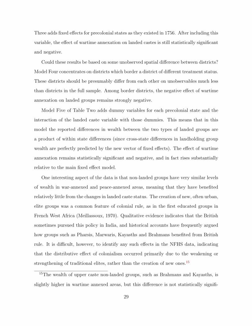
Three adds fixed effects for precolonial states as they existed in 1756. After including this

variable, the effect of wartime annexation on landed castes is still statistically significant

and negative.

Could these results be based on some unobserved spatial difference between districts?

Model Four concentrates on districts which border a district of different treatment status.

These districts should be presumably differ from each other on unobservables much less

than districts in the full sample. Among border districts, the negative effect of wartime

annexation on landed groups remains strongly negative.

Model Five of Table Two adds dummy variables for each precolonial state and the

interaction of the landed caste variable with those dummies. This means that in this

model the reported differences in wealth between the two types of landed groups are

a product of within state differences (since cross-state differences in landholding group

wealth are perfectly predicted by the new vector of fixed effects). The effect of wartime

annexation remains statistically significant and negative, and in fact rises substantially

relative to the main fixed effect model.

One interesting aspect of the data is that non-landed groups have very similar levels

of wealth in war-annexed and peace-annexed areas, meaning that they have benefited

relatively little from the changes in landed caste status. The creation of new, often urban,

elite groups was a common feature of colonial rule, as in the first educated groups in

French West Africa (Meillassoux, 1970). Qualitative evidence indicates that the British

sometimes pursued this policy in India, and historical accounts have frequently argued

how groups such as Pharsis, Marwaris, Kayasths and Brahmans benefited from British

rule. It is difficult, however, to identify any such effects in the NFHS data, indicating

that the distributive effect of colonialism occurred primarily due to the weakening or

strengthening of traditional elites, rather than the creation of new ones.15

15The wealth of upper caste non-landed groups, such as Brahmans and Kayasths, is

slightly higher in wartime annexed areas, but this difference is not statistically signifi-

29

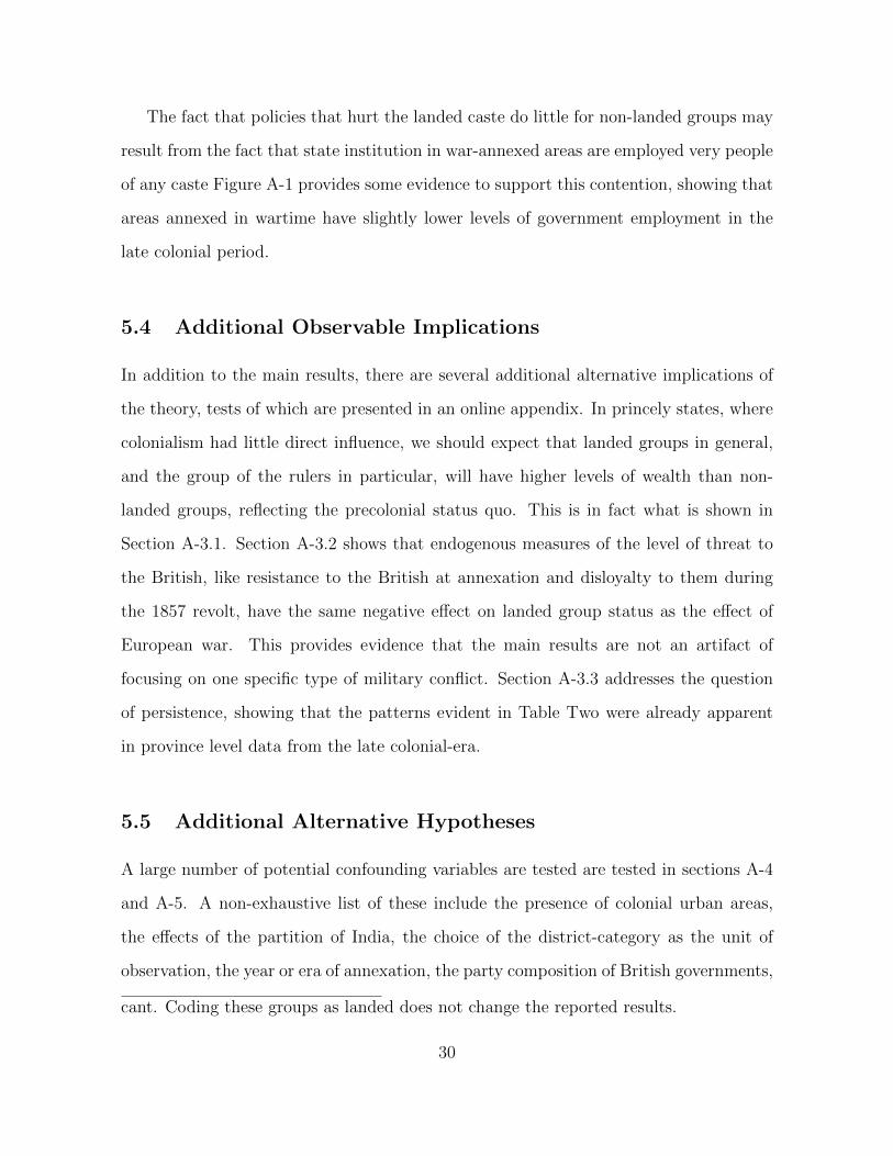
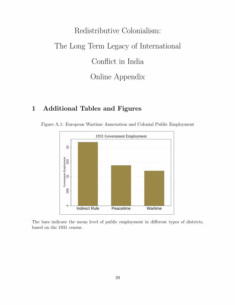
The fact that policies that hurt the landed caste do little for non-landed groups may

result from the fact that state institution in war-annexed areas are employed very people

of any caste Figure A-1 provides some evidence to support this contention, showing that

areas annexed in wartime have slightly lower levels of government employment in the

late colonial period.

5.4 Additional Observable Implications

In addition to the main results, there are several additional alternative implications of

the theory, tests of which are presented in an online appendix. In princely states, where

colonialism had little direct influence, we should expect that landed groups in general,

and the group of the rulers in particular, will have higher levels of wealth than non-

landed groups, reflecting the precolonial status quo. This is in fact what is shown in

Section A-3.1. Section A-3.2 shows that endogenous measures of the level of threat to

the British, like resistance to the British at annexation and disloyalty to them during

the 1857 revolt, have the same negative effect on landed group status as the effect of

European war. This provides evidence that the main results are not an artifact of

focusing on one specific type of military conflict. Section A-3.3 addresses the question

of persistence, showing that the patterns evident in Table Two were already apparent

in province level data from the late colonial-era.

5.5 Additional Alternative Hypotheses

A large number of potential confounding variables are tested are tested in sections A-4

and A-5. A non-exhaustive list of these include the presence of colonial urban areas,

the effects of the partition of India, the choice of the district-category as the unit of

observation, the year or era of annexation, the party composition of British governments,

cant. Coding these groups as landed does not change the reported results.

30

the presence of religious minorities, individual movement between caste groups, the

system of land tenure, the presence of “martial” caste groups, 20th century economic

growth the soil composition (the one dimension on which the wartime-annexed areas

differed from peace annexed areas in the balance test,) and the precolonial wealth of

the territory. None of these factors substantially change the basic results, and very few

seem to differ in their direct effects between the treated and non-treated samples.

6 An Example

The quantitative results show that military threat was an important determinate of

imperial policy, but fail to show what specific policy tools were used to favor or disfavor

landed groups. Some of the more common ones, though difficult to measure, included

the delegation or non-delegation of taxing authority, recruitment into the military and

bureaucracy, and the setting of tax rates. In the case of the North Indian region of Oudh,

however, we can see how the process worked with respect to one particular aspect of

colonial policy with obvious economic importance: The direct confiscation of land from

traditional elites for non-payment of taxes.

Oudh is a particularly useful comparison because it is a case where portions of the

same precolonial state were annexed at different times. The Nawabs of Oudh ruled

a large area of Northern India in the late 18th century, but their ability to conduct

autonomous policy was gradually weakened by the British. This process culminated

in 1801, when the larger half of the Nawabs dominions were ceded to the British (the

“ceded provinces.”) As Figure Three shows, the ceded provinces encircled the territory

that remained under nawabi control. This meant that for a half century, numerous

districts of princely Oudh immediately neighbored districts of British India, though

they had had similar political institutions in the 18th century.

In 1856, the British annexed the remainder of Oudh. It is worth examining the

31

substantial changes in the political situation that had occurred since 1801. In 1801,

Britain was fighting a lonely struggle against Napoleonic France, which had forced it

(in 1797) to suspend payments in gold, and (in 1799) to introduce Europe’s first income

tax. In India, the East India Company was still one player among many, and was still

bracing for a confrontation with the Maratha confederacy. In 1856, by contrast, the

British had just defeated Russia in the Crimean war, and over the past half century had

either annexed or reduced to impotence all the major Indian powers. In Britain itself,

industrialization, still confined to textiles in 1801, had made Britain the world’s leading

economic power.

These different policy imperatives produced very different attitudes towards the

landed castes of Oudh. In the ceded provinces, the colonial state ruthlessly eliminated

much of the former higher aristocracy, who were regarded as useless and dangerous.

This was not accomplished without violence, and some of the recalcitrant landlords saw

their mud forts besieged and taken by the company’s artillery. Even the larger peasant

proprietors, however, suffered from the terms of a series of harsh and inflexibly imple-

mented land tax settlements. In many cases peasant communities were forced into debt

to both the state and urban moneylenders, with the long term result that many lost

their land, often by court-ordered sales (Metcalf 1979). The same result could be seen in

the administrative sphere, where the establishment of company courts and police both

deprived local elites of profitable offices that they had held under the Nawabs but opened

up a smaller set of opportunities for urban professionals. The result was something of a

social revolution in Oudh. As Metcalf (1979) remarks:

By the mid-nineteenth century the face of society in the Doab, once hardlydistinguishable from Oudh, bore little resemblance to its neighbor across theGanges...

Many old landholding families were permanently reduced in influence...Intheir place, and sometimes beside them, rose up new landholding groups—often absentee, city-based or of commercial or service castes. (Metcalf 1979:104, 135).

32

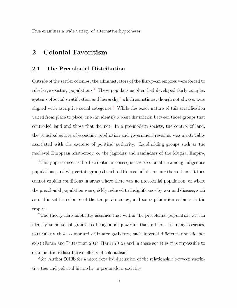
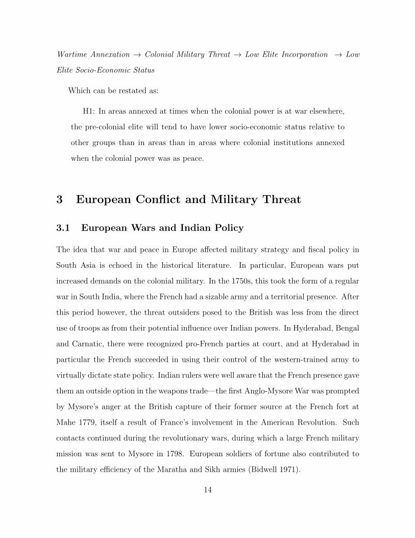
Figure 4: Percentage of Land Owned by Landholding Castes In Oudh, c.1900

53

52

19

16

64

33

28

18

46

45

69

39

76

33

5243

38

17

30 4452

89

17

55

3317

68

33

17

3345

36

45

52

The colored districts were part of Oudh in 1801. The black line is the boundary betweenOudh and British India from 1801 to 1856. The numbers for each district represent thepercentage of land owned by Rajputs, Bhumihars and Jats at the settlement closest to1900. Source: Land Settlement Reports, various years.

In Oudh proper, by contrast, the British adopted a policy that strongly favored

existing landed groups, and confiscations modest relative to the Doab, though some

higher landowners with inadequate title did lose their estates and privileges. Even after

many traditional landed elites had joined the 1857 rebellion, loyal landowners were

restored to their lands and even parts of their judicial responsibilities, a policy that

was echoed across much of British India (Stokes 1978). More generally, the so called

“Oudh Policy” aimed at avoiding disruptions in rural social relations, and emphasized

established landed groups (both big and small) and easy tax assessments.

The results were obvious even in the late colonial period. Figure Four shows the

33

percentage of land in Oudh owned by the three dominant landed castes of the region,

the Rajputs, Bhumihars, and Jats. This figure is based on an original dataset of caste

landholding patterns, itself based on colonial land settlement reports for the period

around 1900.

In general, districts of pre-1856 Oudh show much higher levels of landed caste land-

holding than neighboring districts, which had identical political conditions both before

1801 and after 1856. Some of these contrasts are dramatic. In Pratapgarh, 89% of

the land in 1900 was owned by landed castes, while just across the river in Allahabad,

landed castes owned only 19% of the land. In Allahabad, as in other districts, much of

the difference (31.8%) was made up by urban professional castes.

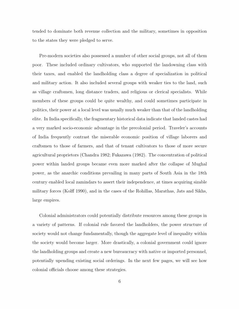
The relationship between colonial-era policy and the poor economic position of the

landed castes in Oudh can be shown even more directly. Figure Five shows the relation-

ship between court-ordered sales of land and the percentage of land owned by landed

castes in UP districts in 1900. Court ordered land sales have a large negative effect

on landed caste land ownership (χ2=-0.38.) Even in a very small sample (n=31) this

correlation is statistically significant at the 5% level.

7 Conclusion

The data presented in the last few sections displays a few simple patterns. Geopolitical

patterns at the time of colonization, in particular the level military and fiscal pressure

on the colonial power, are associated with differences in the socioeconomic status of

groups. In areas where the colonial institutions were created under the threat of a

military challenge sponsored by a rival European power, powerful landed groups suffer

a dramatic reversal of fortune, becoming poor relative to both their former political

inferiors and their coethnics in other regions. In areas annexed in peacetime, precolonial

elites were able to maintain their economic status relatively comfortably. This difference

34

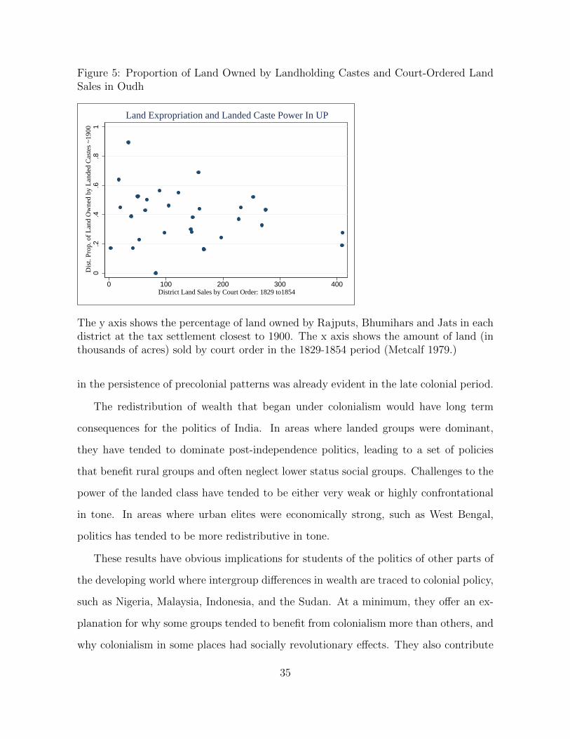
Figure 5: Proportion of Land Owned by Landholding Castes and Court-Ordered LandSales in Oudh

0.2

.4.6

.81

Dis

t. Pr

op. o

f L

and

Ow

ned

by L

ande

d C

aste

s ~1

900

0 100 200 300 400 District Land Sales by Court Order: 1829 to1854

Land Expropriation and Landed Caste Power In UP

The y axis shows the percentage of land owned by Rajputs, Bhumihars and Jats in eachdistrict at the tax settlement closest to 1900. The x axis shows the amount of land (inthousands of acres) sold by court order in the 1829-1854 period (Metcalf 1979.)

in the persistence of precolonial patterns was already evident in the late colonial period.

The redistribution of wealth that began under colonialism would have long term

consequences for the politics of India. In areas where landed groups were dominant,

they have tended to dominate post-independence politics, leading to a set of policies

that benefit rural groups and often neglect lower status social groups. Challenges to the

power of the landed class have tended to be either very weak or highly confrontational

in tone. In areas where urban elites were economically strong, such as West Bengal,

politics has tended to be more redistributive in tone.

These results have obvious implications for students of the politics of other parts of

the developing world where intergroup differences in wealth are traced to colonial policy,

such as Nigeria, Malaysia, Indonesia, and the Sudan. At a minimum, they offer an ex-

planation for why some groups tended to benefit from colonialism more than others, and

why colonialism in some places had socially revolutionary effects. They also contribute

35

to the larger literature on colonialism, by showing that the distributional consequences

of colonialism can be just as substantive and long-lasting as the institutional ones so

commonly discussed in the literature. Finally, it suggests an interesting, and largely

unstudied, set of questions on causes of policy variation within colonial regimes and the

strategic choices made by colonial rulers, showing that the incentives of these rulers are

not just significant, but changeable.

36

Bibliography

Acemoglu, Daron, Simon Johnson, and James Robinson. 2002. “Reversal of fortune.” The

Quarterly Journal of Economics 117.4: 1231-1294.

2001. “The Colonial Origins of Comparative Development” American Economic Review.

Author. 2013a. “Caste Mobilization in Colonial India.” Working Paper.

Author. 2013b. “From Hierarchy to Ethnicity.” Working Paper.

Banerjee, Abhijit and Lakshmi Iyer. 2005. “History, Institutions and Economic Performance”

American Economic Review. 95 (4): 1190-1213.

Bidwell, Shelford. 1971. Swords for hire London: J. Murray.

Chandra, Satish. 1982/“The Standard of Living: The Mughal Empire.” In Raychaudhuri,

Tapan, and Irfan Habib. The Cambridge Economic History of India. Cambridge: Cam-

bridge UP. p.458-471.

Chichester, Henry, and George Burges-Short. 1970. Records and Badges of the British Army.

London: Muller.

Dirks, Nicholas. 2002. Castes of Mind Princeton University Press.

Dodwell, H.H. 1922. British India. V.5. of Rapson, E.J, ed. The Cambridge History of India.

Cambridge: University Press.

Engerman, Stanley and Kenneth Sokoloff. 1998. “Factor Endowments, Inequality, and Paths

of Development Among New World Economies.” NBER Working Paper 9259.

Ertan, Ahran. and Louis Putterman. 2007. “Determinants and Economic Consequences of

Colonization.” Econometric Society conference paper.

Frankel, Francine. and M.S.A. Rao. 1989. Eds. Dominance and state power in modern India

Delhi: Oxford UP.

Fukazawa, H. 1982.“The Standard of Living: South India.” In Raychaudhuri, Tapan, and

Irfan Habib. The Cambridge Economic History of India. Cambridge: Cambridge UP.

p.471-477.

Furnivall, John. 1948. Colonial policy and practice CUP Archive.

37

Hariri, Jacob Gerner. 2012. “The Autocratic Legacy of Early Statehood.” American Political

Science Review 106(3):471-494.

Horowitz, David. 1985.Ethnic Groups in Conflict. Cambridge: Cambridge UP.

International Institute for Population Sciences. 2000. National Family Health Survey 1998-99

Final Report. http://www.measuredhs.com/pubs/pdf/FRIND2/FRIND2.pdf

Iyer, Lakshmi. (2010) “Direct versus indirect colonial rule in India: Long-term consequences.’

’The Review of Economics and Statistics 92.4 : 693-713.

Kolff, D.H.A. 1990. Naukar, Rajput, and Sepoy Cambridge: Cambridge University Press.

Lee, Alexander and Kenneth Schultz. 2012. “Comparing British and French Colonial Legacies”

Quarterly Journal of Political Science, 7: 146.

Mahoney, James. 2010. Colonialism and Postcolonial Development Cambridge UP.

Metcalf, Thomas. 1979. textit Land, landlords, and the British RajUniversity of California

Press.

Mukherjee, Shivaji. 2013. “Colonial Origins of Maoist Insurgency in India.” APSA meeting

paper.

Nunn, Nathan. 2009. “The importance of history for economic development.” No. w14899.

NBER.

Schwartzberg, Joseph, and Shiva Gopal Bajpai. 1978. A Historical Atlas of South Asia.

Chicago: University of Chicago Press.

Srinivas. M.N. 1966. Social Change in Modern India. Berkeley: University of California Press.

Stokes, Eric. 1978.The Peasant and the Raj Cambridge: Cambridge UP.

Streets, Heather. 2004. ’ Martial Races Manchester UP.

Yapp, Malcolm. 1987 “British perceptions of the Russian threat to India.” Modern Asian

Studies. 21.4: 647-665.

38

Redistributive Colonialism:

The Long Term Legacy of International

Conflict in India

Online Appendix

1 Additional Tables and Figures

Figure A.1: European Wartime Annexation and Colonial Public Employment

0.0

05.0

1.0

15.0

2 G

over

nmen

t Em

ploy

men

t

Indirect Rule Peacetime Wartime

1931 Government Employment

The bars indicate the mean level of public employment in different types of districts,based on the 1931 census.

39

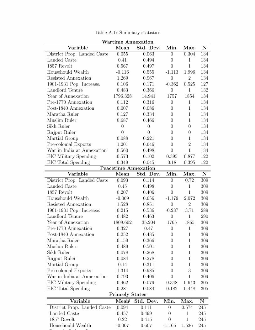
Table A.1: Summary statistics

Wartime AnnexationVariable Mean Std. Dev. Min. Max. N

District Prop. Landed Caste 0.055 0.063 0 0.304 134Landed Caste 0.41 0.494 0 1 1341857 Revolt 0.567 0.497 0 1 134Househould Wealth -0.116 0.555 -1.113 1.996 134Resisted Annexation 1.269 0.967 0 2 1341901-1931 Pop. Increase. 0.106 0.171 -0.362 0.525 127Landlord Tenure 0.483 0.366 0 1 132Year of Annexation 1796.328 14.941 1757 1854 134Pre-1770 Annexation 0.112 0.316 0 1 134Post-1840 Annexation 0.007 0.086 0 1 134Maratha Ruler 0.127 0.334 0 1 134Muslim Ruler 0.687 0.466 0 1 134Sikh Ruler 0 0 0 0 134Rajput Ruler 0 0 0 0 134Martial Group 0.088 0.221 0 1 134Pre-colonial Exports 1.201 0.646 0 2 134War in India at Annexation 0.560 0.498 0 1 134EIC Military Spending 0.573 0.102 0.395 0.877 122EIC Total Spending 0.349 0.045 0.18 0.395 122

Peacetime AnnexationVariable Mean Std. Dev. Min. Max. N

District Prop. Landed Caste 0.093 0.114 0 0.72 309Landed Caste 0.45 0.498 0 1 3091857 Revolt 0.207 0.406 0 1 309Househould Wealth -0.069 0.656 -1.179 2.072 309Resisted Annexation 1.528 0.851 0 2 3091901-1931 Pop. Increase. 0.215 0.536 -0.287 3.71 289Landlord Tenure 0.482 0.463 0 1 290Year of Annexation 1809.602 35.204 1765 1865 309Pre-1770 Annexation 0.327 0.47 0 1 309Post-1840 Annexation 0.252 0.435 0 1 309Maratha Ruler 0.159 0.366 0 1 309Muslim Ruler 0.489 0.501 0 1 309Sikh Ruler 0.078 0.268 0 1 309Rajput Ruler 0.084 0.278 0 1 309Martial Group 0.14 0.311 0 1 309Pre-colonial Exports 1.314 0.985 0 3 309War in India at Annexation 0.793 0.406 0 1 309EIC Military Spending 0.462 0.079 0.348 0.643 305EIC Total Spending 0.281 0.084 0.182 0.448 305

Princely States

Variable Mean Std. Dev. Min. Max. NDistrict Prop. Landed Caste 0.094 0.111 0 0.574 245Landed Caste 0.457 0.499 0 1 2451857 Revolt 0.22 0.415 0 1 245Househould Wealth -0.007 0.607 -1.165 1.536 245Princely Ruling Group 0.227 0.393 0 1 2451901-1931 Pop. Increase. 0.18 0.302 -0.287 1.696 241Maratha Ruler 0.184 0.388 0 1 245Muslim Ruler 0.204 0.404 0 1 245Sikh Ruler 0.045 0.208 0 1 245Rajput Ruler 0.441 0.498 0 1 245Martial Group 0.186 0.369 0 1 245Pre-colonial Exports 0.588 0.694 0 2 245

40

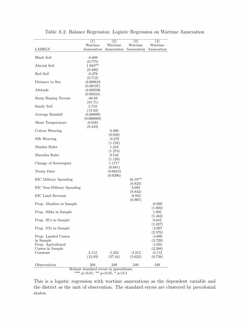
Table A.2: Balance Regression: Logistic Regression on Wartime Annexation

(1) (2) (3) (4)Wartime Wartime Wartime Wartime

LABELS Annexation Annexation Annexation Annexation

Black Soil -0.808(0.775)

Aluvial Soil 1.083**(0.480)

Red Soil -0.378(0.712)

Distance to Sea -0.000616(0.00197)

Altitude -0.000596(0.00316)

Steep Sloping Terrain -88.68(81.71)

Sandy Soil 5.719(14.82)

Average Rainfall -0.000995(0.000869)

Mean Temperature -0.0581(0.443)

Cotton Weaving 0.460(0.949)

Silk Weaving -0.278(1.132)

Muslim Ruler 1.216(1.274)

Maratha Ruler 0.542(1.120)

Change of Sovereignty 1.171*(0.681)

Treaty Date -0.00415(0.0206)

EIC Military Spending 16.19**(6.823)

EIC Non-Military Spending 3.095(8.842)

EIC Land Revenue -8.943(6.907)

Prop. Muslims in Sample -0.999(1.802)

Prop. Sikhs in Sample 1.895(5.462)

Prop. SCs in Sample 0.644(1.927)

Prop. STs in Sample -2.997(2.570)

Prop. Landed Castes -4.899in Sample (3.729)Prop. Agricultural -1.055Castes in Sample (2.288)Constant 2.112 5.232 -3.212 -0.112

(12.93) (37.44) (5.622) (0.738)

Observations 204 249 240 249Robust standard errors in parentheses

*** p<0.01, ** p<0.05, * p<0.1

This is a logistic regression with wartime annexations as the dependent variable andthe district as the unit of observation. The standard errors are clustered by precolonialstates.

2 History

In precolonial India the possession of land was closely linked, and indeed inextricably

confused, with the exercise of the political power. In the Mughal Empire, which ruled

much of South Asia until the early 18th century, officeholders were rewarded with jagirs

(grants of land taxation) rather than fixed salaries, while at a lower level the ownership

rights of various classes of village proprietors were closely associated with the right to

collect and pay land taxes, and collectively referred to as zamindari. Land, being the

primary economic asset in an agrarian society, was also associated with economic status.

These differences in political and economic status were in turn closely associated

with status within the caste system. Within each region, a members of few groups

held a large proportion of both land and political power, and these groups tended to be

regarded as “clean” or high-status within the context of the caste system. This dynamic

was to a large extent self-reinforcing: Politically powerful groups were able to engage in

the rituals and behaviors associated with high status, and this in turn enhanced their

political power (Bayly 1999.)

In the princely states that occupied a large portion of India, the arrival of the

British did not alter this social order, merely imposing a “subsidiary alliance,” by which

the Indian prince renounced an independent foreign policy. This left the rural elite

of these areas, the jagirdars and zamindars, in possession of their land and a sizable

portion of their fiscal and legal autonomy, and the conflict between them and the court

was a theme of politics in many princely states (Ramusack 2004). In princely capitals,

the bureaucracy and court remained recruited from a narrow set of backgrounds, and

particularly from the relatives and coethnics of the ruler himself (Ernst and Pati 2007).

There is considerable debate with the historiography of colonial India over the extent

to which British rule displaced traditional rural elites in directly ruled areas. Certainly

for many landlords the colonial period represented an opportunity, which enabled them

42

to dispense with expensive military obligations, while using the newly established court

system to enforce demands on their tenants. Some more localized zamindar groups were

able to take advantage of the opportunities available in the company’s military, and the

enhanced physical security introduced by the company’s government (Bayly 1983; Cohn

1960)

However, there is strong evidence that in some areas of Bengal and Uttar Pradesh,

traditional rural elites were not able to survive the transition to British rule. Many

were simply caught on the wrong side of the wars of conquest: Those elites too closely

associated with opposition to the British, or with general lawlessness, such as the Pindari

chieftains of Bundelkhand, were generally ignored in the redistribution of land that

accompanied the conquest. Even if they succeeded in retaining their position, the early

colonial land settlements often disfavored the existing elite. This was less because of

the nature of the land tenure institutions themselves than because of the high level of

the land revenue demand and the consistent way in which the company’s institutions

enforced it, quite unlike the flexible and highly negotiable nature of late Mughal land

taxation. Many landholders both large and small fell into arrears and had their estates

sold, often to urbanites closely connected to the British administration (Marshall 1976).

Even those landowners who retained their land found that it did not bring them political

power as readily as it once had. Their private armies and forts were dismantled by the

British, who gradually replaced their judicial functions with an institutionalized court

system. In UP, for instance, the former ruling dynasties of Benares, Farrukhabad and

Hatras saw their land revenue rights replaced by government pensions, and their taxing

powers over trade abolished completely (Bayly 1983: 269). This in turn reduced, and

at times eliminated, the ability of these rulers to support large courts or bureaucracies.

The major beneficiaries of these institutions were the clerical and urban castes of

these regions, previously subordinate but now able to buy the estates of their former

superiors, attain positions in the colonial bureaucracy, or get jobs as lawyers or as

43

factors for European firms. Brahmans in both Tamil Nadu and Bengal would be known

throughout the colonial period both for their high levels of wealth and their close links

to the state, as would the Kayasth caste of Northern India, who were already closely

associated with government service.

Even before the eighteenth century was out, some colonial officials felt that they

may have gone too far in attacking traditional rural elites, who were now seen as useful

bulwarks of the rural social order rather than threatening rivals. The result was a set

of policies intended to strengthen existing social forces, most notably a less aggressive

approach to land revenue assessment, and an attempt to protect indigenous landlords

and cultivators from moneylenders and forced sale by auction (Metcalf 1979). While

early manifestation of this policy orientation, like the permanent settlement of the land

revenue of Bengal, tended to favor larger landlords, later policy initiative concentrated

on peasant communities. In areas with ryotwari or patidari land tenure systems, many

upper peasants gained land revenue rights, while tenants gained institutionalized pro-

tections (Stokes 1978). In the 20th century, tax assessments became increasingly light,

and rural loan schemes attempted to end “leakage” of land to urban moneylenders.

2.1 Bengal and Punjab

The contrast between the elite strengthening and elite-weakening types of colonialism can

be seen most clearly when by comparing Bengal and Punjab . Bengal, mostly annexed

during the Seven Years war, is widely regarded as being an extreme and enduring case

of colonialism redistribution towards non-landed groups. Punjab, annexed during the

long peace of the 1840s, is widely regarded as experiencing colonial policies blatantly

biased towards the landed castes.

Bengal was the first part of India conquered by the British. Annexation was a

gradual, process, but most of the province was annexed by the company during the

1750s. This coincided with the Seven Years War in Europe, which was paralleled by a

44

full dress conflict between the British and French in South India, and a vicious proxy

war for influence within Bengal. During these early years of British rule, their military

position was highly insecure—at the start of the war, Calcutta had been besieged and

taken by the Nawab. This insecurity may explain the ruthless attitude that the British

adopted towards the traditional landed groups

As in other parts of Eastern India, the British implemented a land tenure regime

that granted land tenure rights to large landlords. However Bengal stood apart from

other parts of the East such as Bihar, in the highness of the tax demand and the

ruthlessness and inflexibility with which it was implemented. The combination of high

and inflexible demands and unpredictable harvest was bankruptcy for the Muslim and

Rajput landlords of Bengal, the late 18th century saw the expropriation of virtually

every major landowner by court order (Marshall 1976). Their replacements were often

from traditionally non-landed groups such as the Brahmans and Kayasths, who used

wealth earned in trade with the British to buy estates.

The other mechanism by which these non-landed groups gained influence was through

the rapidly expanding colonial administration. Unlike their urban competitors, tradi-

tional landlords found it difficult to adjust to the demands of the colonial bureaucracy,

which valued literacy over descent or military prowess. Unlike in other parts of India,

the colonial state made little attempt to accommodate them. The results were clear:

According to the 1911 census, members of the urban literate castes made up 83.7%

of the gazetted civil servants in Bengal, and 54.6% of police and army officers. These

non-landed upper castes, the bhadralok, also took on a dominant, and enduring, role in

the cultural life of the province (Government of India 1918; Jaffrelot and Kumar 2009,

Frankel and Rao 1989).

Punjab, annexed in 1846, was the last major independent power in India, and was

annexed at the height of British power worldwide. While the British had had to fight a

stiff battle to destroy the Sikh Kingdom, they quickly lost any fear they may have had of

45

the Sikhs, and in fact during the 1857 rebellion came to view them as a useful bulwark

against the recalcitrant elites of other areas of India. The trust extended so far that

Punjabis came to dominate the colonial army. In this context, the British developed a

set of stereotypes (the “martial races” theory) that emphasized the racial superiority of

Punjabis over other groups (Streets 2004).

For these reasons, the pro-peasant turn in British policy was most pronounced in the

Punjab, where the landholding groups were able to maintain some of their traditional

political power even within the context of direct rule. In this province the British

established a system of administration, the “Punjab System,” that deemphasized formal

institutions in favor of the informal ones of Sikh and Jat peasant communities and

individual relationships with British officials (Yong 2005). Not only was the colonial

state small, but it was not dominated by the urban castes: In 1911, Brahmans comprised

38.9% of the educated professionals in UP, but only 5.9% in Punjab.

British favoritism towards landholding groups culminated in the Punjab Alienation

of Land Act (1901). Motivated by the fear that urban groups were acquiring too much

economic power, the act banned the transfer of land to members of groups defined

as non-agricultural, the act banned the acquisition of land by non-agricultural groups

(Casson 2010). This was coupled with a massive investment in irrigation, which made

the Punjab the most agriculturally dynamic part of India in the late colonial period, and

immensely strengthened the social position of the Jats and Sikhs, the largest peasant

groups.

3 Additional Implications

3.1 Princely States

Hypothesis One made no distinction between the maintenance of native elites in their

existing positions through mechanisms such as indirect rule or the active incorporation

46

of these elites within western-style institutions. Both policies have similar observable

implications, since they will allow the landholding elites to maintain or expand their

existing economic advantages.

The results reported above deal only with directly ruled areas, since it is only pos-

sible to analyze the effect of military threat at the time of annexation in areas that

were actually annexed. In addition, we have strong reason to believe that indirectly

ruled areas might differ substantially from directly ruled areas in their level of precolo-

nial political and economic development (Gerring et. al 2011, Iyer 2007). However,

Hypothesis One is agnostic as to whether a militarily secure colonial state will choose

to conciliate landed elites by maintaining their institutions intact and separate (as in

indirect rule) or by assimilating their personnel and practices into European institutions.

Indirect rule may thus be an alternative pathway by which landed groups may benefit

from colonialism, or at least minimize their losses.

However, there are two reasons why we might expect the positive effect of indirect

rule on landed castes to be more ambiguous and limited than the effect of direct rule

by a militarily secure colonial state. Firstly, the majority of the princely states of India,

like indirectly ruled polities in other parts of the world, tended to centralize power in the

hands of a single ruler and his friends and relatives, and distributed resources through

informal channels that marginalized groups not connected to the ruler. The Raput

rulers of Rajasthan, for instance, distributed resources to Rajputs and a few Brahmans,

excluding the large and relatively wealthy groups of Jat cultivators. We might thus

expect the effects of indirect rule on the landed class as a whole to be mixed, with the

ruler coethnics benefiting at the expense of other landed groups.

Secondly, many indirectly ruled areas were somewhat isolated from the social changes

that might allow the advantages of their elites to persist in the post-independence world.

Indirectly ruled areas, for examples, had higher levels of literacy than directly ruled ar-

eas, but (predictably) lower levels of literacy in English. Similarly, the economy of most

47

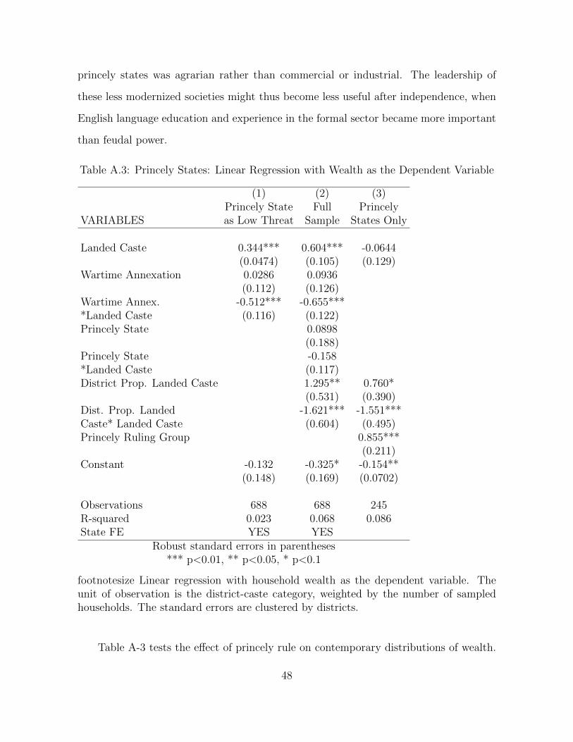
princely states was agrarian rather than commercial or industrial. The leadership of

these less modernized societies might thus become less useful after independence, when

English language education and experience in the formal sector became more important

than feudal power.

Table A.3: Princely States: Linear Regression with Wealth as the Dependent Variable

(1) (2) (3)Princely State Full Princely

VARIABLES as Low Threat Sample States Only

Landed Caste 0.344*** 0.604*** -0.0644(0.0474) (0.105) (0.129)

Wartime Annexation 0.0286 0.0936(0.112) (0.126)

Wartime Annex. -0.512*** -0.655****Landed Caste (0.116) (0.122)Princely State 0.0898

(0.188)Princely State -0.158*Landed Caste (0.117)District Prop. Landed Caste 1.295** 0.760*

(0.531) (0.390)Dist. Prop. Landed -1.621*** -1.551***Caste* Landed Caste (0.604) (0.495)Princely Ruling Group 0.855***

(0.211)Constant -0.132 -0.325* -0.154**

(0.148) (0.169) (0.0702)

Observations 688 688 245R-squared 0.023 0.068 0.086State FE YES YES

Robust standard errors in parentheses*** p<0.01, ** p<0.05, * p<0.1

footnotesize Linear regression with household wealth as the dependent variable. Theunit of observation is the district-caste category, weighted by the number of sampledhouseholds. The standard errors are clustered by districts.

Table A-3 tests the effect of princely rule on contemporary distributions of wealth.

48

Model One codes princely states as having been annexed at times of European peace,

while Model Two codes the princely states separately, adding measures of wartime an-

nexation. Whichever model is chosen, wartime annexation has a significant and negative

effect on landed castes, with the effect being somewhat larger than that estimated in

Table Three. The effect of princely rule on landed castes, however, is small and statically

insignificant. One possible reason for this is suggested in Model Three, which examines

the effect of indirect rule on the caste group of the ruler. District-Castes from the same

caste category as the state’s ruler tend to have a higher level of wealth than members

of the same caste without this advantage. This would tend to support the hypothesis

that, even if indirect rule does not benefit the landed class as a whole, it does tend to

benefit the ruler’s relatives and dependents.

3.2 Endogenous Measures of Military Threat

The models in Table Two use as their independent variable a determinate of military

threat, geopolitical conditions in Europe, which has the attractive property of being

relatively independent of local conditions in India. However, there are a number of

factors associated with the level of military and fiscal threat experienced by the British,

and their treatment of landed groups, that do not have this property. In particular,

colonial powers might be particularly disposed to view landed groups as threatening if

they fought the colonial power, either during the annexation process or subsequently.

Similarly, groups are that fought for the colonial power might subsequently be viewed

as non-threatening, quite independent of their social or geographical position.

The most obvious endogenous measure of military threat is whether there was a mil-

itary confrontation with the British at the time of annexation. In such areas, colonial

officials had actual evidence of the potential hostile intent of the local elite, and the pun-

ishment of defeated opponents provided an opportunity for the destruction of existing

political arrangements. The policy of punishing defeated opponents was by no means

49

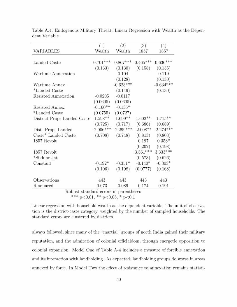
Table A.4: Endogenous Military Threat: Linear Regression with Wealth as the Depen-dent Variable

(1) (2) (3) (4)VARIABLES Wealth Wealth 1857 1857

Landed Caste 0.701*** 0.867*** 0.465*** 0.636***(0.133) (0.130) (0.158) (0.135)

Wartime Annexation 0.104 0.119(0.128) (0.130)

Wartime Annex. -0.623*** -0.634****Landed Caste (0.149) (0.130)Resisted Annexation -0.0205 -0.0117

(0.0605) (0.0605)Resisted Annex. -0.160** -0.135**Landed Caste (0.0755) (0.0727)District Prop. Landed Caste 1.598** 1.699** 1.602** 1.715**

(0.725) (0.717) (0.686) (0.689)Dist. Prop. Landed -2.006*** -2.299*** -2.008** -2.274***Caste* Landed Caste (0.708) (0.748) (0.813) (0.803)1857 Revolt 0.197 0.358*

(0.202) (0.198)1857 Revolt 3.561*** 3.333****Sikh or Jat (0.573) (0.626)Constant -0.192* -0.351* -0.140* -0.303*

(0.106) (0.198) (0.0777) (0.168)

Observations 443 443 443 443R-squared 0.073 0.089 0.174 0.191

Robust standard errors in parentheses*** p<0.01, ** p<0.05, * p<0.1

Linear regression with household wealth as the dependent variable. The unit of observa-tion is the district-caste category, weighted by the number of sampled households. Thestandard errors are clustered by districts.

always followed, since many of the “martial” groups of north India gained their military

reputation, and the admiration of colonial officialdom, through energetic opposition to

colonial expansion. Model One of Table A-4 includes a measure of forcible annexation

and its interaction with landholding. As expected, landholding groups do worse in areas

annexed by force. In Model Two the effect of resistance to annexation remains statisti-

50

cally significant, though its inclusion does not change the effect of wartime annexation.

Both endogenous and exogenous factors it seems, determine the redistributive effect of

colonialism.

The rebellion of 1857, which temporarily destroyed colonial institutions in most

of Northern India, had far reaching impact on colonial policy towards rural Indians.

In particular, groups that stayed loyal to the British, notably the Jat and Sikhs of

the Punjab, came to be viewed more positively than groups that were conspicuous in

the rebellion, notably Rajputs, Muslims and Brahmans from Oudh and Bihar (Hibbert

1978). Model Three of Table Four examines whether being in a district affected by the

rebellion, had a negative effect on the landed castes. In areas affected by the mutiny,

coded based on Schwartzenburg and Bajpai (1978), groups widely thought to have stayed

loyal to the British (Sikhs and Jats) are wealthier than their coethnics elsewhere. In these

areas members of groups widely thought to have participated in the rebellion, Brahmans,

Rajputs, Upper Caste Muslims, and Bhumihars, do more poorly than members of these

groups elsewhere though this difference is not statistically significant. In Model Four we

see that controlling for the effect of the rebellion has no effect of wartime annexation on

landed group wealth.

3.3 Colonial Data

If the differences in wealth that we observe in 1998 can be traced to differences in the

policy of the colonial state at the time of annexation, we should expect them to already be

evident in the late colonial period. Indeed, we should expect differences between groups

to have been larger in this period, since the economic status of groups will have been

unaffected by the policies of the post-colonial government. However, if these differences

are a product of government favoritism, we should expect them to be concentrated in

goods closely associated with the colonial government, in particular employment in the

government itself.

51

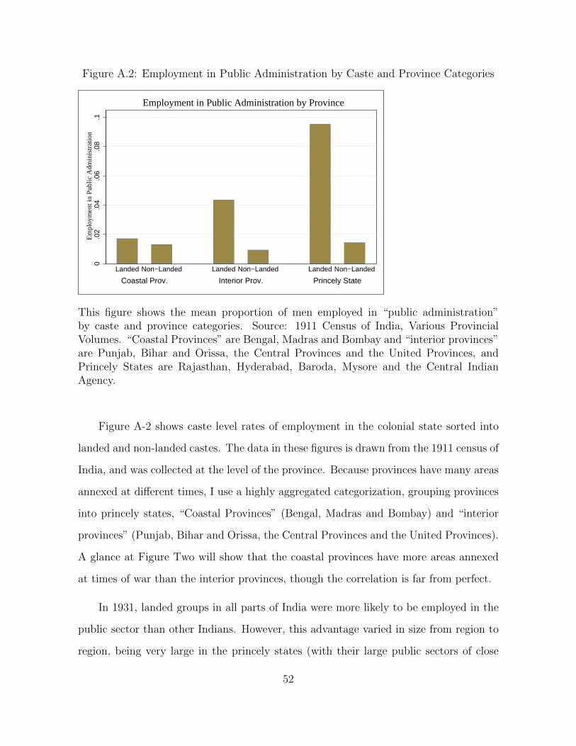
Figure A.2: Employment in Public Administration by Caste and Province Categories

0.0

2.0

4.0

6.0

8.1

Em

ploy

men

t in

Publ

ic A

dmin

istr

atio

n

Coastal Prov. Interior Prov. Princely State

Landed Non−Landed Landed Non−Landed Landed Non−Landed

Employment in Public Administration by Province

This figure shows the mean proportion of men employed in “public administration”by caste and province categories. Source: 1911 Census of India, Various ProvincialVolumes. “Coastal Provinces” are Bengal, Madras and Bombay and “interior provinces”are Punjab, Bihar and Orissa, the Central Provinces and the United Provinces, andPrincely States are Rajasthan, Hyderabad, Baroda, Mysore and the Central IndianAgency.

Figure A-2 shows caste level rates of employment in the colonial state sorted into

landed and non-landed castes. The data in these figures is drawn from the 1911 census of

India, and was collected at the level of the province. Because provinces have many areas

annexed at different times, I use a highly aggregated categorization, grouping provinces

into princely states, “Coastal Provinces” (Bengal, Madras and Bombay) and “interior

provinces” (Punjab, Bihar and Orissa, the Central Provinces and the United Provinces).

A glance at Figure Two will show that the coastal provinces have more areas annexed

at times of war than the interior provinces, though the correlation is far from perfect.

In 1931, landed groups in all parts of India were more likely to be employed in the

public sector than other Indians. However, this advantage varied in size from region to

region, being very large in the princely states (with their large public sectors of close

52

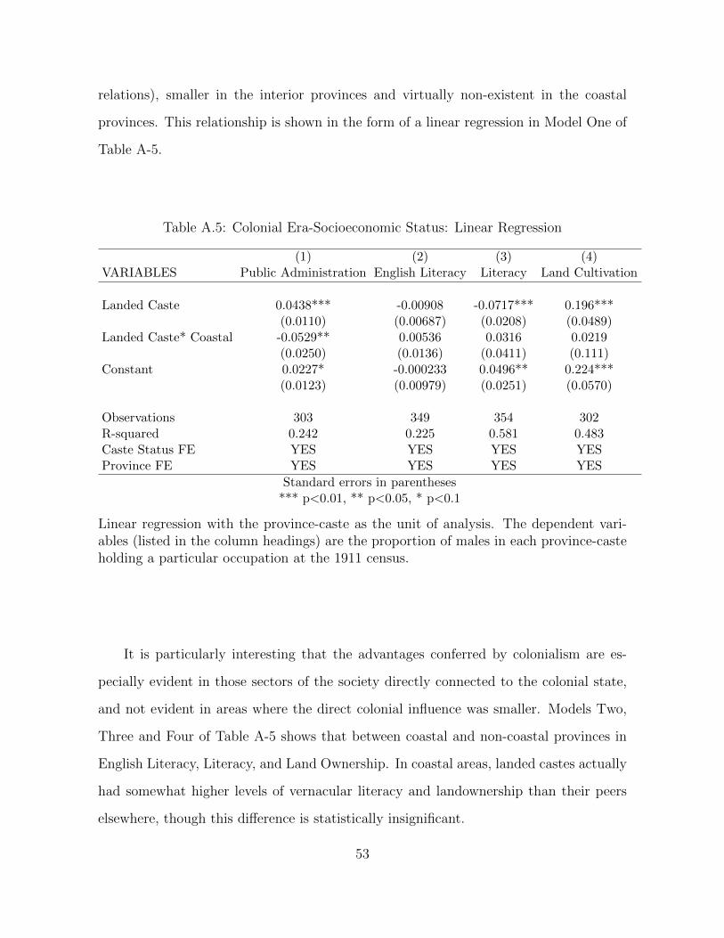
relations), smaller in the interior provinces and virtually non-existent in the coastal

provinces. This relationship is shown in the form of a linear regression in Model One of

Table A-5.

Table A.5: Colonial Era-Socioeconomic Status: Linear Regression

(1) (2) (3) (4)VARIABLES Public Administration English Literacy Literacy Land Cultivation

Landed Caste 0.0438*** -0.00908 -0.0717*** 0.196***(0.0110) (0.00687) (0.0208) (0.0489)

Landed Caste* Coastal -0.0529** 0.00536 0.0316 0.0219(0.0250) (0.0136) (0.0411) (0.111)

Constant 0.0227* -0.000233 0.0496** 0.224***(0.0123) (0.00979) (0.0251) (0.0570)

Observations 303 349 354 302R-squared 0.242 0.225 0.581 0.483Caste Status FE YES YES YES YESProvince FE YES YES YES YES

Standard errors in parentheses*** p<0.01, ** p<0.05, * p<0.1

Linear regression with the province-caste as the unit of analysis. The dependent vari-ables (listed in the column headings) are the proportion of males in each province-casteholding a particular occupation at the 1911 census.

It is particularly interesting that the advantages conferred by colonialism are es-

pecially evident in those sectors of the society directly connected to the colonial state,

and not evident in areas where the direct colonial influence was smaller. Models Two,

Three and Four of Table A-5 shows that between coastal and non-coastal provinces in

English Literacy, Literacy, and Land Ownership. In coastal areas, landed castes actually

had somewhat higher levels of vernacular literacy and landownership than their peers

elsewhere, though this difference is statistically insignificant.

53

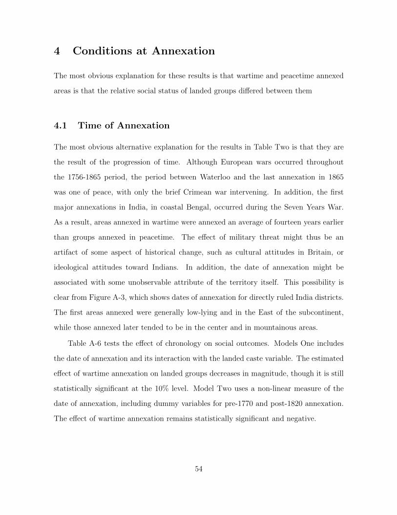
4 Conditions at Annexation

The most obvious explanation for these results is that wartime and peacetime annexed

areas is that the relative social status of landed groups differed between them

4.1 Time of Annexation

The most obvious alternative explanation for the results in Table Two is that they are

the result of the progression of time. Although European wars occurred throughout

the 1756-1865 period, the period between Waterloo and the last annexation in 1865

was one of peace, with only the brief Crimean war intervening. In addition, the first

major annexations in India, in coastal Bengal, occurred during the Seven Years War.

As a result, areas annexed in wartime were annexed an average of fourteen years earlier

than groups annexed in peacetime. The effect of military threat might thus be an

artifact of some aspect of historical change, such as cultural attitudes in Britain, or

ideological attitudes toward Indians. In addition, the date of annexation might be

associated with some unobservable attribute of the territory itself. This possibility is

clear from Figure A-3, which shows dates of annexation for directly ruled India districts.

The first areas annexed were generally low-lying and in the East of the subcontinent,

while those annexed later tended to be in the center and in mountainous areas.

Table A-6 tests the effect of chronology on social outcomes. Models One includes

the date of annexation and its interaction with the landed caste variable. The estimated

effect of wartime annexation on landed groups decreases in magnitude, though it is still

statistically significant at the 10% level. Model Two uses a non-linear measure of the

date of annexation, including dummy variables for pre-1770 and post-1820 annexation.

The effect of wartime annexation remains statistically significant and negative.

54

Figure A.3: Dates of Annexation of Indian Districts

DISTRICT1991ANNEXDATE

1757176017631765176617781788179217931799180018011802180318051815181718181823182618301832183518381839184018461849185318541856185818601865

These results echo the raw data on annexation dates, shown as Table A-7. No

matter whether annexation was early or late chronologically, areas annexed in wartime

tend to have a larger landed caste economic advantage. In particular, those landed

groups annexed in the 1764-77 period of peace have a .36 higher wealth advantage than

those annexed just a few years before during the Seven Years War. Landed groups whose

district was annexed in 1816-53 have a .47 higher wealth advantage than those annexed

during the Napoleonic Wars.

55

4.2 War in India

Another possible explanation for these results is that the effect we observe of European

wars actually reflects military conditions in India. In this formulation, colonial percep-

tions of military threat are influenced by whether the Company was fighting a war in

India, rather than the enhanced threat resulting from these enemies being cobelligerent

with European powers. As we have seen this is unlikely to alter the main results given

that military conflict was endemic in colonial India (72% of Indian districts were forcibly

conquered, and an identical 72% were annexed in a year the company was fighting a war

somewhere in India) and that the few peaceful years are uncorrelated with European

conflicts. Nevertheless, this hypothesis is tested in Table A-6.

Model Three includes controls for the existence of conflict in India as a whole, and

Model Four controls for indigenous resistance to British Conquest. Consistent with

the theoretical expectation, the interactions of both these variables with landedness are

statistically significant (at the 10% level) indicating that the linkage between military

conflict and elite impoverishment works for Indian conflicts as well as European ones.

However, the inclusion of these variables does not change the effect of European Conflicts

on landed groups. This is not unsurprising. While conflict with indigenous powers was

very common and mildly concerning, it was external conflict and external aid that made

these conflicts much more threatening.

4.3 British Government and Finance

A closely related concern is that European war and the relative social position of landed

castes are spuriously related due to the existence of different schools of policymaking in

British politics. An “aggressive” ministry, in this view, would be ideologically inclined

both to become involved in European wars and to adopt aggressive policies towards

Indian elites. This concern is particularly troubling because during periods of European

56

war England was governed primarily by the Tory party–indeed the wars of the 18th

century were a key issue in the evolution of the English party system. Models One and

Two of Table A-8 test this hypothesis. Model One examines whether controlling for Tory

Party government reduces the effect of wartime annexation (with Whig and coalition

governments as the excluded category.) Model Two examines the effect of “aggressive”

ministries, coded as those that were in power at the onset of a European war. The effect

of wartime annexation on landed castes remains statically significant and negative, after

the inclusion of these controls. The coefficient of the interaction of the cabinet variables

with caste landedness has a value close to zero, indicating that cabinet composition has

little direct redistributive impact.

One of the predictions of Section Two was that financial pressure on the colonial

government might be one of the mechanisms by which European conflict influences colo-

nial policy. It might be, however, that fiscal constraints influence policy independent of

European conflict. Models Three and Four of Table A-8 Test this hypothesis. Model

Three includes controls for the total levels of EIC spending and military spending, nor-

malized by revenue. This captures the idea that colonial policy might change relative to

fiscal needs, with the state trying to increase revenue and increase expenditure. Models

Four controls for the level of land revenue relative to total revenue. This accounts for the

possibility that the results are driven by the Company’s gradual shift from dependence

on land revenue to dependence on other types of taxation, which might affect their pol-

icy towards landed groups. While the fiscal measures are correlated with district-level

levels of wealth, they do not seem to have any substantial effect on the relative position

of landed and non-landed castes. More importantly, their inclusion does not alter the

negative effect of wartime annexation on landed castes.

57

5 Alternative Explanations

5.1 Alternative Specifications

Table A-9 tests whether the results are robust to the use of alternative strategies for

coding the key variables and organizing the analysis. Models One and Two recode

two components of the key independent variable. Model One includes controls for the

date at which a precolonial state signed a subsidiary treaty with the British (usually

earlier than the date of annexation). Its inclusion does not alter the effect of wartime

annexation. Model Two redefines landed castes to include the large group of castes that

were traditionally associated with agriculture (based on the 1911 census) but did not

have an aristocratic or military tradition. The effect of wartime annexation on these

agricultural castes is large and negative, and very similar in size to the effect on the

smaller group of landed castes, indicating that the coding of this variable is not driving

the results.

Models Three and Four changes the unit of observation from the district caste

category to the district. Model Three tests a simple form of this hypothesis, comparing

landed castes in areas annexed at times of European war to landed castes in areas

annexed at times of European peace. Landed castes in the peacetime-annexed areas are

significantly better off than their coethnics elsewhere, with the average landed district-

jati having a quarter of a standard deviation higher wealth in a peacetime-annexed area

than in a wartime-annexed area. Model Four takes as its dependent variable the district-

level differences between landed and non-landed castes. Wartime annexation is a strong

negative predictor of these differences, with the economic advantage of landed castes

being much smaller in wartime annexed areas than elsewhere.

58

While the use of the district-caste category as the unit of observation matches treat-

ment to measurement, it ignores the clustered design used in the collection of the individ-

ual data. Model Five reruns the basic model using the full dataset, with the individual

as the unit of observation. In this model, the standard errors are clustered by survey

cluster, and weighted by the original survey weights. The results in this model are vir-

tually unchanged from thus in table two, indicating that the results are uninfluenced

by the choice of the unit of observation. Model Six further develop this by using the

district-jati as the unit of observation, again without effect on the results.

5.2 Robustness Checks

Table A-10 examines whether the effects in Table Two are being driven by a particular

subsection of the data. Model One excludes the modern states that have no areas

annexed at time of war, which include Rajasthan, Maharashtra, Kerala, Punjab, Madhya

Pradesh and Bihar. In these regions in which there were no-treated areas, it is impossible

to identify within-state treatment effects. Despite the smaller sample size, the estimates

effects of wartime annexation are still statistically significant and negative, echoing the

results in Table Two.

59

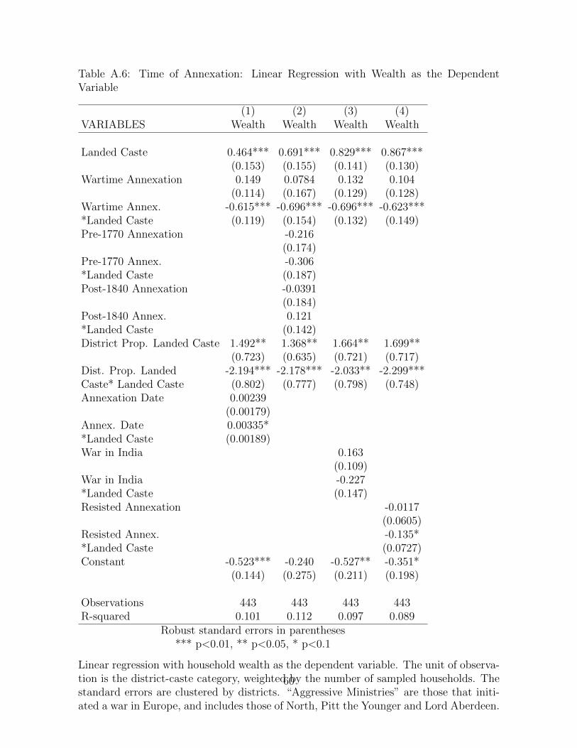
Table A.6: Time of Annexation: Linear Regression with Wealth as the DependentVariable

(1) (2) (3) (4)VARIABLES Wealth Wealth Wealth Wealth

Landed Caste 0.464*** 0.691*** 0.829*** 0.867***(0.153) (0.155) (0.141) (0.130)

Wartime Annexation 0.149 0.0784 0.132 0.104(0.114) (0.167) (0.129) (0.128)

Wartime Annex. -0.615*** -0.696*** -0.696*** -0.623****Landed Caste (0.119) (0.154) (0.132) (0.149)Pre-1770 Annexation -0.216

(0.174)Pre-1770 Annex. -0.306*Landed Caste (0.187)Post-1840 Annexation -0.0391

(0.184)Post-1840 Annex. 0.121*Landed Caste (0.142)District Prop. Landed Caste 1.492** 1.368** 1.664** 1.699**

(0.723) (0.635) (0.721) (0.717)Dist. Prop. Landed -2.194*** -2.178*** -2.033** -2.299***Caste* Landed Caste (0.802) (0.777) (0.798) (0.748)Annexation Date 0.00239

(0.00179)Annex. Date 0.00335**Landed Caste (0.00189)War in India 0.163

(0.109)War in India -0.227*Landed Caste (0.147)Resisted Annexation -0.0117

(0.0605)Resisted Annex. -0.135**Landed Caste (0.0727)Constant -0.523*** -0.240 -0.527** -0.351*

(0.144) (0.275) (0.211) (0.198)

Observations 443 443 443 443R-squared 0.101 0.112 0.097 0.089

Robust standard errors in parentheses*** p<0.01, ** p<0.05, * p<0.1

Linear regression with household wealth as the dependent variable. The unit of observa-tion is the district-caste category, weighted by the number of sampled households. Thestandard errors are clustered by districts. “Aggressive Ministries” are those that initi-ated a war in Europe, and includes those of North, Pitt the Younger and Lord Aberdeen.

60

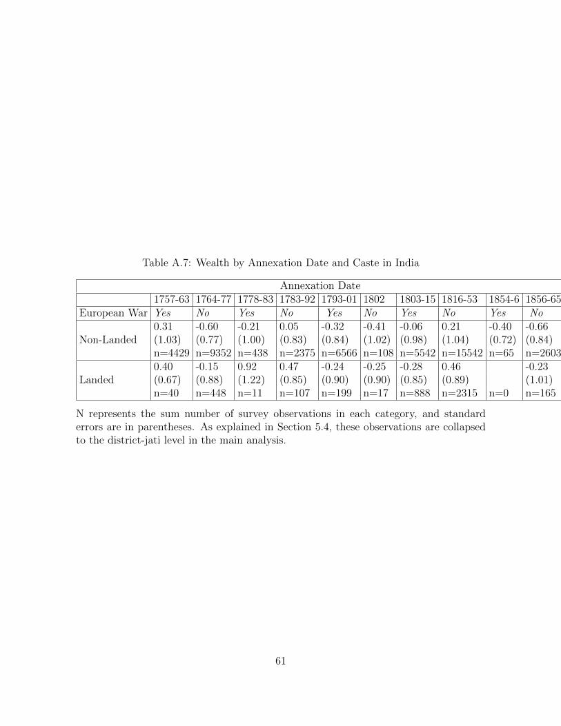
Table A.7: Wealth by Annexation Date and Caste in India

Annexation Date1757-63 1764-77 1778-83 1783-92 1793-01 1802 1803-15 1816-53 1854-6 1856-65

European War Yes No Yes No Yes No Yes No Yes No

Non-Landed0.31 -0.60 -0.21 0.05 -0.32 -0.41 -0.06 0.21 -0.40 -0.66(1.03) (0.77) (1.00) (0.83) (0.84) (1.02) (0.98) (1.04) (0.72) (0.84)n=4429 n=9352 n=438 n=2375 n=6566 n=108 n=5542 n=15542 n=65 n=2603

Landed0.40 -0.15 0.92 0.47 -0.24 -0.25 -0.28 0.46 -0.23(0.67) (0.88) (1.22) (0.85) (0.90) (0.90) (0.85) (0.89) (1.01)n=40 n=448 n=11 n=107 n=199 n=17 n=888 n=2315 n=0 n=165

N represents the sum number of survey observations in each category, and standarderrors are in parentheses. As explained in Section 5.4, these observations are collapsedto the district-jati level in the main analysis.

61

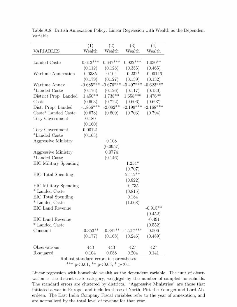
Table A.8: British Annexation Policy: Linear Regression with Wealth as the DependentVariable

(1) (2) (3) (4)VARIABLES Wealth Wealth Wealth Wealth

Landed Caste 0.613*** 0.647*** 0.922*** 1.030**(0.112) (0.128) (0.355) (0.465)

Wartime Annexation 0.0385 0.104 -0.232* -0.00146(0.179) (0.127) (0.139) (0.132)

Wartime Annex. -0.685*** -0.676*** -0.497*** -0.623****Landed Caste (0.176) (0.126) (0.117) (0.130)District Prop. Landed 1.450** 1.738** 1.658*** 1.476**Caste (0.603) (0.722) (0.606) (0.697)Dist. Prop. Landed -1.866*** -2.082** -2.199*** -2.168***Caste* Landed Caste (0.678) (0.809) (0.703) (0.794)Tory Government 0.180

(0.160)Tory Government 0.00121*Landed Caste (0.163)Aggressive Ministry 0.108

(0.0957)Aggressive Ministry 0.0774*Landed Caste (0.146)EIC Military Spending 1.254*

(0.707)EIC Total Spending 2.112**

(0.822)EIC Military Spending -0.735* Landed Caste (0.815)EIC Total Spending 0.184* Landed Caste (1.068)EIC Land Revenue -0.915**

(0.452)EIC Land Revenue -0.491* Landed Caste (0.552)Constant -0.353** -0.381** -1.217*** 0.506

(0.177) (0.168) (0.246) (0.489)

Observations 443 443 427 427R-squared 0.104 0.088 0.204 0.141

Robust standard errors in parentheses*** p<0.01, ** p<0.05, * p<0.1

Linear regression with household wealth as the dependent variable. The unit of obser-vation is the district-caste category, weighted by the number of sampled households.The standard errors are clustered by districts. “Aggressive Ministries” are those thatinitiated a war in Europe, and includes those of North, Pitt the Younger and Lord Ab-erdeen. The East India Company Fiscal variables refer to the year of annexation, andare normalized by the total level of revenue for that year.

62

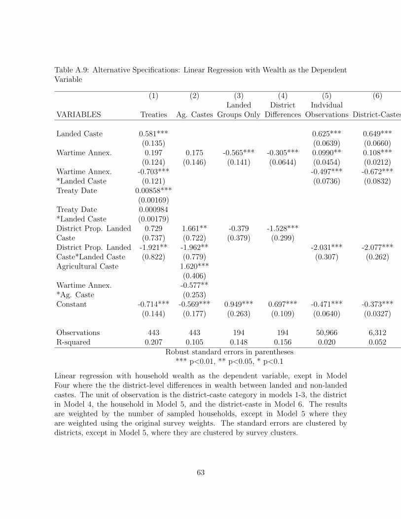
Table A.9: Alternative Specifications: Linear Regression with Wealth as the DependentVariable

(1) (2) (3) (4) (5) (6)Landed District Indvidual

VARIABLES Treaties Ag. Castes Groups Only Differences Observations District-Castes

Landed Caste 0.581*** 0.625*** 0.649***(0.135) (0.0639) (0.0660)

Wartime Annex. 0.197 0.175 -0.565*** -0.305*** 0.0990** 0.108***(0.124) (0.146) (0.141) (0.0644) (0.0454) (0.0212)

Wartime Annex. -0.703*** -0.497*** -0.672****Landed Caste (0.121) (0.0736) (0.0832)Treaty Date 0.00858***

(0.00169)Treaty Date 0.000984*Landed Caste (0.00179)District Prop. Landed 0.729 1.661** -0.379 -1.528***Caste (0.737) (0.722) (0.379) (0.299)District Prop. Landed -1.921** -1.962** -2.031*** -2.077***Caste*Landed Caste (0.822) (0.779) (0.307) (0.262)Agricultural Caste 1.620***

(0.406)Wartime Annex. -0.577***Ag. Caste (0.253)Constant -0.714*** -0.569*** 0.949*** 0.697*** -0.471*** -0.373***

(0.144) (0.177) (0.263) (0.109) (0.0640) (0.0327)

Observations 443 443 194 194 50,966 6,312R-squared 0.207 0.105 0.148 0.156 0.020 0.052

Robust standard errors in parentheses*** p<0.01, ** p<0.05, * p<0.1

Linear regression with household wealth as the dependent variable, exept in ModelFour where the the district-level differences in wealth between landed and non-landedcastes. The unit of observation is the district-caste category in models 1-3, the districtin Model 4, the household in Model 5, and the district-caste in Model 6. The resultsare weighted by the number of sampled households, except in Model 5 where theyare weighted using the original survey weights. The standard errors are clustered bydistricts, except in Model 5, where they are clustered by survey clusters.

63

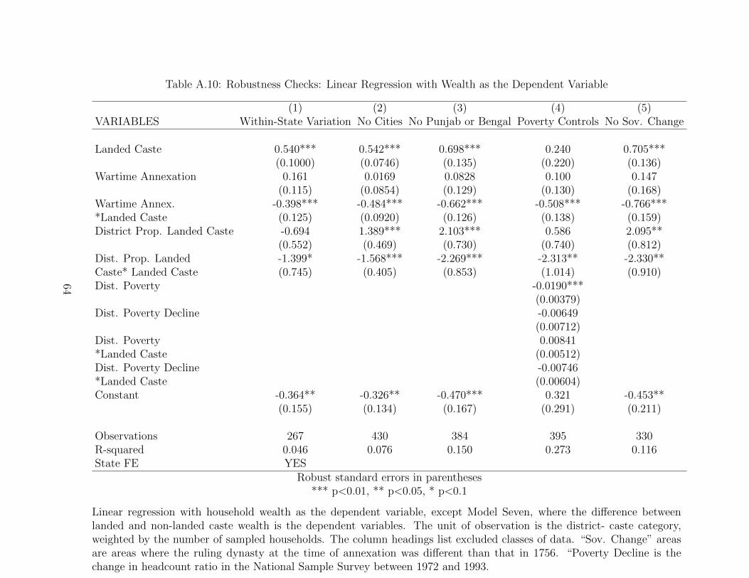
Table A.10: Robustness Checks: Linear Regression with Wealth as the Dependent Variable

(1) (2) (3) (4) (5)VARIABLES Within-State Variation No Cities No Punjab or Bengal Poverty Controls No Sov. Change

Landed Caste 0.540*** 0.542*** 0.698*** 0.240 0.705***(0.1000) (0.0746) (0.135) (0.220) (0.136)

Wartime Annexation 0.161 0.0169 0.0828 0.100 0.147(0.115) (0.0854) (0.129) (0.130) (0.168)

Wartime Annex. -0.398*** -0.484*** -0.662*** -0.508*** -0.766****Landed Caste (0.125) (0.0920) (0.126) (0.138) (0.159)District Prop. Landed Caste -0.694 1.389*** 2.103*** 0.586 2.095**

(0.552) (0.469) (0.730) (0.740) (0.812)Dist. Prop. Landed -1.399* -1.568*** -2.269*** -2.313** -2.330**Caste* Landed Caste (0.745) (0.405) (0.853) (1.014) (0.910)Dist. Poverty -0.0190***

(0.00379)Dist. Poverty Decline -0.00649

(0.00712)Dist. Poverty 0.00841*Landed Caste (0.00512)Dist. Poverty Decline -0.00746*Landed Caste (0.00604)Constant -0.364** -0.326** -0.470*** 0.321 -0.453**

(0.155) (0.134) (0.167) (0.291) (0.211)

Observations 267 430 384 395 330R-squared 0.046 0.076 0.150 0.273 0.116State FE YES

Robust standard errors in parentheses*** p<0.01, ** p<0.05, * p<0.1

Linear regression with household wealth as the dependent variable, except Model Seven, where the difference betweenlanded and non-landed caste wealth is the dependent variables. The unit of observation is the district- caste category,weighted by the number of sampled households. The column headings list excluded classes of data. “Sov. Change” areasare areas where the ruling dynasty at the time of annexation was different than that in 1756. “Poverty Decline is thechange in headcount ratio in the National Sample Survey between 1972 and 1993.

64

It is possible that the observed differences in landed caste status are a product of

the fact that two of the three main port cities of colonial India, Calcutta and Madras,

were annexed at times of European war, and (like the third major city, Bombay) have

very high levels of wealth. Model Two of table A-10 excludes these three cities. The

effect of wartime annexation is still statistically significant and negative in this model.

One implicit assumption of the attempt to measure direct effects of the colonial

period in the 1990s is that there have been no major social changes in the intervening

period to move groups from one place to another, or to fundamentally alter the economic

status of landholding groups. The one event in South Asian history that might fit

these criteria is the 1947 partition of India, which resulted in widespread population

movements to and from Pakistan. Model Three of Table A-10 accounts for this possibility

by excluding the states of Punjab, Haryana and West Bengal, the areas most affected

by the flow of refugees. The effect of wartime annexation is virtually identical with the

exclusion of these areas, indicating that the effect of partition, or any other element of

the political economy of these states, on the main results was minimal.

Another source of post-treatment bias is the economic growth that transformed some

areas of India in the late 20th century. Model Four includes control for the absolute

level of poverty in 1970s India and its change over the next two decades. Neither

of these variables has a significant effect on groups wealth, and their inclusion does

not substantively change the relationship between landed group wealth and wartime

annexation

The definitions of precolonial state used in these models are based on the status

quo in a single year, 1756. However, 18th century Indian politics was very unstable,

and in many cases the ruling dynasty in 1756 was different from that ruling at the time

of annexation. Model Five of Table A-10 excludes areas in which the polity controlling

the area at the time it fell within the British sphere of influence was different from

that controlling the area in 1756. In areas where control of the state was shifting,

65

we might expect the connection between the landholding elite and the power structure

to be weaker, or at least more complicated. However, excluding these areas appears

to somewhat increase the estimated negative effect of wartime annexation on landed

groups.

5.3 Alternative Definitions of Caste

Could the results be distorted by the presence of religious minorities, whose relationship

to the caste categories used in the analysis is at times antagonistic?16 In particular,

could missionary-induced conversion the Christianity be driving variation in the socio-

economic status of groups, as it appears to do for some African groups? Model One of

Table A-11 excludes non-Hindus, with little effect on the results.

Even if units are taken as constant, the membership of groups is not, as individuals

opportunistically recatagorize themselves into higher castes (Rao and Ban 2007; Casson

2010.) There is some reason to think that these movements may cause us too substan-

tially underestimate the effect of colonial redistribution. If colonial resources tended to

flow to a particular groups, this would create an incentive for poor individuals to join

these groups, thus lowering both their average wealth and the estimated redistributive

effect of colonialism.17

Model Two of Table A-11 examines the effect of these changes, using a unique panel

dataset of population changes of Indian groups in the colonial era 18 It includes as a

control variable the proportional change in a castes population between the 1901 and

16At the NFHS, some members of religious minorities reported their caste, while others

reported their religion. The later choice was coded as non-landed in the main analysis.17Consistent with this theory, the landed caste category is slightly higher in war-

annexed than in peace annexed areas.18For a further description of this data, which is based on the colonial era censuses,

see Author 2013a.

66

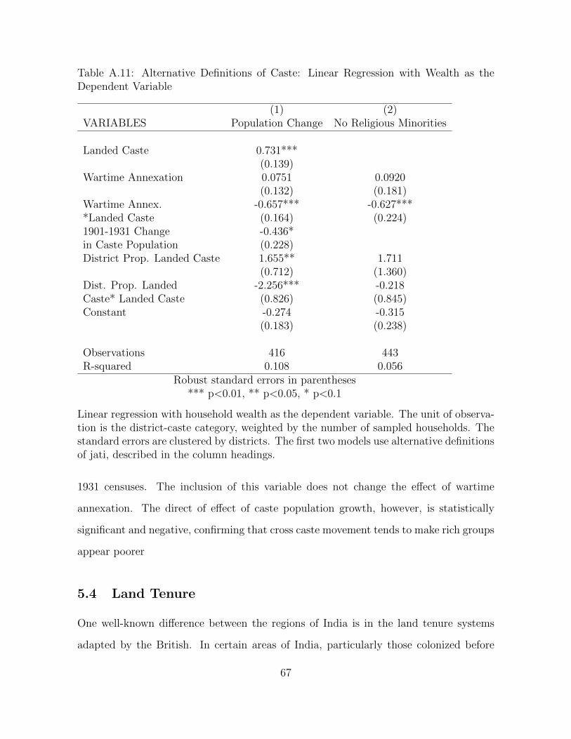
Table A.11: Alternative Definitions of Caste: Linear Regression with Wealth as theDependent Variable

(1) (2)VARIABLES Population Change No Religious Minorities

Landed Caste 0.731***(0.139)

Wartime Annexation 0.0751 0.0920(0.132) (0.181)

Wartime Annex. -0.657*** -0.627****Landed Caste (0.164) (0.224)1901-1931 Change -0.436*in Caste Population (0.228)District Prop. Landed Caste 1.655** 1.711

(0.712) (1.360)Dist. Prop. Landed -2.256*** -0.218Caste* Landed Caste (0.826) (0.845)Constant -0.274 -0.315

(0.183) (0.238)

Observations 416 443R-squared 0.108 0.056

Robust standard errors in parentheses*** p<0.01, ** p<0.05, * p<0.1

Linear regression with household wealth as the dependent variable. The unit of observa-tion is the district-caste category, weighted by the number of sampled households. Thestandard errors are clustered by districts. The first two models use alternative definitionsof jati, described in the column headings.

1931 censuses. The inclusion of this variable does not change the effect of wartime

annexation. The direct of effect of caste population growth, however, is statistically

significant and negative, confirming that cross caste movement tends to make rich groups

appear poorer

5.4 Land Tenure

One well-known difference between the regions of India is in the land tenure systems

adapted by the British. In certain areas of India, particularly those colonized before

67

the 1790s, the British established a system known as zamindari tenure, in which the

right to pay land revenue, and by extension property rights in land, were transferred

to landlords and politically-connected elites. In other areas of India, they adapted two

alternative systems, village-based (in which the revenue was the responsibility of the

cultivators within each village jointly), and ryotwari (in which the cultivators paid their

share directly to the state). The differences among these systems have been posited as

a source of regional inequality in India, and as a cause of the enrichment of rural elites

(Banerjee and Iyer 2005.)

Models One and Two of Table A-12 examine whether the wartime annexation is

purely an effect of land tenure systems, including as a control the percentage of land

farmed by landlords (taken from Banerjee and Iyers data) and it’s interaction with the

landed caste variable. Consistent with Banerjee and Iyer’s findings, the direct effect of

zamindari tenure is substantial and negative, though landlord tenure does not appear

to affect the relative standing of landed and non-landed castes, or to change the effect

of wartime annexation. This is also true in Model Two, where the sample is confined to

districts where over 30% of the land was cultivated by landlords.

This non-effect of land tenure systems on caste inequalities seems less strange when

we examine how zamindari tenure actually worked, and the great variation in the way

land tenure systems implement. In particular, there was substantial variation both

across areas and across time in the tax rates the British imposed on zamindars and their

willingness to use the legal process to evict non-paying tenants. Where tax rates were low

and the eviction process rarely used, colonialism could have a profoundly conservative

effect, strengthening the hold of rural landlords. Where tax rates were high and eviction

common, colonialism could affect a revolution in land tenure, replacing established local

families with urban elites, often closely associated with the colonial state (Metcalf 1979).

These differences in implementation, driven by the colonial state’s need to conciliate local

elites, could thus be far more significant than differences in the legal and institutional

68

setting.

5.5 Martial Races

In the late 19th century, the British concentrated their military recruitment, which had

previously drawn on a fairly broad section of the landed castes, on a few groups thought

to possess martial virtues, including loyalty to the Empire. These groups, notably Jats,

Rajputs, Gurkhas and Sikhs, have been thought to have received substantial social

benefits from their service. This very conscious favoritism tends to support rather than

the weaken the theory developed in Section Two, since the favored groups tended to be

landed elites in areas that were annexed late in colonial history or were never annexed at

all. The most long-lasting example of such favoritism, the Gurkhas, came from outside

India entirely. While favoritism towards the martial races tends to demonstrate the

theory rather than refute it, it is interesting to see if the differences we observe in the

wealth of landed groups is a function of this specific type of colonial favoritism. Model

Three of Table A-12 includes a binary variable of martial groups, defined as groups that

had more than ten companies of infantry from that group in the Indian Army in 1922.

While “martial” status appears to be associated with higher levels of wealth in 1998, its

inclusion does not alter the effect of military threat at the time of annexation.

5.6 Revenue and Resources

It is possible that colonial policy was determined as much by the resources available

in the territory as by its level of military threat. While these differences should be

neutralized in a large sample, it is possible that colonial economic development was

associated with times of war. This does not appear to be the case in Figure A-13,

which shows East India Company exports to India relative to periods of European war.

The trend of exports seem unrelated to European conflict, with substantial peaks and

69

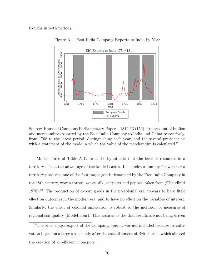
troughs in both periods.

Figure A.4: East India Company Exports to India by Year

500

1000

1500

2000

2500

Exp

orts

to In

dia

in 0

00s

of P

ound

s

1751 1761 1771 1781 1791 1801 1811Year

European ConflictEIC Exports

EIC Exports to India 1754−1811

Source: House of Commons Parliamentary Papers. 1812-13 (152) “An account of bullionand merchandize exported by the East India Company to India and China respectively,from 1708 to the latest period; distinguishing each year, and the several presidencies:with a statement of the mode in which the value of the merchandize is calculated.”

Model Three of Table A-12 tests the hypothesis that the level of resources in a

territory effects the advantage of the landed castes. It includes a dummy for whether a

territory produced one of the four major goods demanded by the East India Company in

the 18th century, woven cotton, woven silk, saltpeter and pepper, taken from (Chaudhuri

1978).19 The production of export goods in the precolonial era appears to have little

effect on outcomes in the modern era, and to have no effect on the variables of interest.

Similarly, the effect of colonial annexation is robust to the inclusion of measures of

regional soil quality (Model Four). This assures us the that results are not being driven

19The other major export of the Company, opium, was not included because its culti-

vation began on a large a scale only after the establishment of British rule, which allowed

the creation of an efficient monopoly.

70

by the presence of alluvial soils, the only significant difference between the war and

peacetime annexed areas in the balance tests.

Additional Works Cited

Bayly, C. A. 1983. Rulers, Townsmen, and Bazaars : North Indian Society In the Age of

British Expansion, 1770-1870. Cambridge [Cambridgeshire]: Cambridge University

Press.

Bayly, Susan. 1999. Caste, Society and Politics in India Cambridge UP, Cambridge.

Cassan, Guilhem. 2010. British law and caste identity manipulation in colonial India:

the Punjab Alienation of Land Act. Indian Statistical Institute Coference Paper.

2010.

Cohn, Bernard S. 1960. “The Initial British Impact on India: A Case Study of the

Benares Region.” The Journal of Asian Studies , Vol. 19, No. 4 (Aug., 1960), pp.

418-431.

Ernst, Waltraud, and Biswamoy Pati. 2007. India’s Princely States : People, Princes

and Colonialism. London: Routledge,

Gerring, John, et al. 2011. ”An Institutional Theory of Direct and Indirect Rule.”

World Politics. 63.3: 377-433.

Henige, David P. 2004.Princely states of India Orchid Press.

Iversen, Vegard, Richard Palmer-Jones, and Kunal Sen. 2012. “On the colonial origins of

agricultural development in India: a re-examination of Banerjee and Iyer,’.” History,

Institutions and Economic Performance. (August 22).

Marshall, Peter James. 1976. East Indian fortunes: the British in Bengal in the eigh-

teenth century. Oxford: Clarendon Press.

Ramusack, Barbara N. 2004. The Indian Princes and Their States. Cambridge, UK:

Cambridge University Press.

Rao, Vijayendra and Radu Ban. 2007.“The Political Construction of Caste in South

India.” World Bank Working Paper.

71

Yong, Tan Tai. 2005.The Garrison State Delhi: SAGE Publications.

72

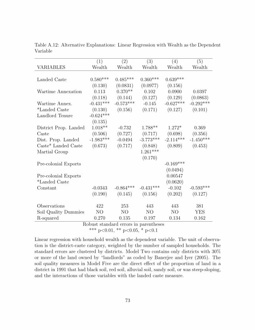
Table A.12: Alternative Explanations: Linear Regression with Wealth as the DependentVariable

(1) (2) (3) (4) (5)VARIABLES Wealth Wealth Wealth Wealth Wealth

Landed Caste 0.580*** 0.485*** 0.360*** 0.639***(0.130) (0.0831) (0.0977) (0.156)

Wartime Annexation 0.113 0.370** 0.102 0.0900 0.0397(0.118) (0.144) (0.127) (0.129) (0.0863)

Wartime Annex. -0.431*** -0.573*** -0.145 -0.627*** -0.292****Landed Caste (0.130) (0.156) (0.171) (0.127) (0.101)Landlord Tenure -0.624***

(0.135)District Prop. Landed 1.018** -0.732 1.788** 1.272* 0.369Caste (0.506) (0.727) (0.717) (0.698) (0.356)Dist. Prop. Landed -1.983*** -0.0494 -3.773*** -2.114*** -1.450***Caste* Landed Caste (0.673) (0.717) (0.848) (0.809) (0.453)Martial Group 1.261***

(0.170)Pre-colonial Exports -0.169***

(0.0494)Pre-colonial Exports 0.00547*Landed Caste (0.0620)Constant -0.0343 -0.864*** -0.431*** -0.102 -0.593***

(0.190) (0.145) (0.156) (0.202) (0.127)

Observations 422 253 443 443 381Soil Quality Dummies NO NO NO NO YESR-squared 0.270 0.135 0.197 0.134 0.162

Robust standard errors in parentheses*** p<0.01, ** p<0.05, * p<0.1

Linear regression with household wealth as the dependent variable. The unit of observa-tion is the district-caste category, weighted by the number of sampled households. Thestandard errors are clustered by districts. Model Two contains only districts with 30%or more of the land owned by “landlords” as coded by Banerjee and Iyer (2005). Thesoil quality measures in Model Five are the direct effect of the proportion of land in adistrict in 1991 that had black soil, red soil, alluvial soil, sandy soil, or was steep-sloping,and the interactions of those variables with the landed caste measure.

73