Redistribution and Social Insurance

Mikhail GolosovPrinceton

Maxim TroshkinCornell

Aleh Tsyvinski∗

Yale

October 2013

Abstract

We study optimal redistribution and insurance with dynamic idiosyn-

cratic shocks. We show the forces that determine the optimal labor dis-

tortions and derive closed form expressions for their limiting behavior. The

labor distortions for high shocks are driven by labor elasticity and higher mo-

ments of the shock process; the labor distortions for low shocks are driven by

the persistence of the shock process, redistributive objectives, and by past

distortions. We calibrate our model using newly available estimates of idio-

syncratic shocks and find that optimal labor distortions are approximately

U-shaped, saving distortions are flat except for low realization of shocks.

∗The previous draft of this paper was circulated under a title "Optimal Dynamic Taxes".

We thank Stefania Albanesi, Fernando Alvarez, V.V. Chari, Dirk Krueger, Larry Jones,

Igor Livshits, Stephen Morris, James Poterba, Emmanuel Saez, Ali Shourideh, Nancy Qian,

Hongda Xiao, Pierre Yared, and numerous seminar and conference audiences. Marianne

Bruins, James Duffy and Nicolas Werquin provided outstanding research assistance. Go-

losov and Tsyvinski thank EIEF for hospitality and NSF for support. Troshkin thanks

Minneapolis Fed for hospitality and support. Tsyvinski thanks IMES of the Bank of Japan

and John Simon Guggenheim Foundation.

A sizeable New Dynamic Public Finance (NDPF) literature studies redis-

tribution and social insurance in lifecycle models.1 This literature extends the

classic Mirrlees equity-effi ciency trade-off to dynamic settings, where agents

are heterogeneous in their abilities and receive stochastic shocks over lifetime.

Despite a significant progress achieved in recent years, still relatively little

is known about the general forces determining optimal allocations and their

qualitative and quantitative properties. This paper makes a step toward filling

that gap.

We study a lifecycle economy with individuals who are ex ante hetero-

geneous in their abilities and experience idiosyncratic shocks to the abilities

over time. We make two contributions. Our theoretical contribution char-

acterizes key forces determining the size of optimal distortions and derives

transparent, easily interpretable expressions for the labor distortions, for high

and low realizations of idiosyncratic shocks, in terms of empirically measurable

parameters and the moments of the stochastic shock process. Our quantitat-

ive contribution computes optimal labor and savings distortions in a lifecycle

model, calibrated to newly available data on the labor earning process for a

random sample of 10 percent of U.S. working-age male population. The data

set allows highly accurate estimates of the moments of the stochastic process

(Guvenen et al. (2013)), which emerge from our analysis as key parameters

determining the properties of the optimum.

Most of our theoretical analysis focuses on characterizing the properties of

optimal labor distortions, or wedges, between marginal utility of consumption

and leisure. We show that the labor distortion in a given period has two

components: an intratemporal component that provides insurance against new

1See, for example, Golosov, Kocherlakota and Tsyvinski (2003) or reviews in Golosov,

Tsyvinski and Werning (2006) and Kocherlakota (2010).

1

shocks in that period, and an intertemporal component that relaxes incentive

constraints in the previous periods and helps reduce the costs of insurance

provision against idiosyncratic shocks. The intratemporal component has the

same general structure as optimal labor distortions in static models, such as

Mirrlees (1971) and Saez (2001). The intertemporal component is new to

dynamic settings. It is driven by a specific form of a likelihood ratio of the

stochastic idiosyncratic shock process, which is equal to the persistence of

the shock when preferences are separable between consumption and labor,

and when idiosyncratic shocks are drawn from a log-normal distribution (or a

mixture of log-normals).

We show that intra- and intertemporal components affect the high and the

low realizations of shocks differently. In a benchmark model with separable

consumption and leisure, the size of the labor distortions for high realizations

of shocks is driven primarily by the intratemporal component, while the size

of the labor distortions for the low realizations is primarily driven by the in-

tertemporal component. We use this insight to derive explicit expressions for

the labor distortions conditional on high and low realizations of idiosyncratic

shocks. The labor distortions for high shocks depend on the Frisch elasticity

of labor supply and on a measure of the dispersion of shocks - variance when

shocks are drawn from a log-normal distribution, kurtosis when shocks are

drawn from a mixture of normals, or a Pareto tail parameter when shocks are

drawn from an asymptotically Pareto distribution. The labor distortions for

low realizations of shocks are proportional to shock persistence, past labor dis-

tortions, and the size of the fall in consumption due to the shock. In addition

to providing transparent, easily interpretable expressions, the decomposition

into low and high realizations facilitates an understanding of quantitative res-

ults by shedding light on how different parameters affect the size and shape of

2

the distortions. The expressions imply, for instance, that the planner’s redis-

tribution objective primarily affects the labor distortions for low, but not for

high shocks.

We also show that an additional force emerges in dynamic economies when

consumption and labor are complements. Complementarity exacerbates the

distortion and, as a result, motivates the social planner to shift from intratem-

poral provision of incentives to the intertemporal provision, especially for the

high skilled. We show that for a range of preferences with complementarities

and no income effects, such as those in Greenwood, Hercowitz and Huffman

(1988), this implies that the optimal labor distortions for the highly skilled

individuals are very low (and asymptotically zero) and savings distortions are

quantitatively high, independently of the nature of the underlying shock pro-

cess.

Our analysis emphasizes the importance of the properties of the distribu-

tion from which individuals draw idiosyncratic shocks, and, in particular, its

higher moments. In the quantitative analysis of a life cycle, we use newly

available estimates of the idiosyncratic labor income process from a high qual-

ity administrative U.S. data by Guvenen et al. (2013) and Guvenen, Ozkan

and Song (2013). This idiosyncratic shock process implies that optimal labor

distortions are approximately U-shaped when preferences are separable and

isoelastic. The dip in the distortion is around the expected realization of the

shock, conditional on past information. Savings distortions are approximately

flat, except for the low skilled. As explained by our theoretical analysis, both

the shape and the size of optimal labor distortions depend significantly on

the kurtosis of the idiosyncratic shock, which, in Guvenen et al. (2013), is

estimated to be over 20 for prime-age males. In contrast, a commonly used as-

sumption of log-normal shocks implies an approximately flat labor distortions

3

with much higher optimal savings distortions.

A number of papers are related to our work. Our theoretical and quantit-

ative analyses are built on the recursive approach developed in Kapicka (2013)

and Pavan, Segal and Toikka (2010). An important contribution of Farhi and

Werning (2013) derives a formula describing the dynamics of labor income

taxes in continuous and discrete cases, provides a simulation of a lifecycle

economy, and develops additional insights using a continuous time approach.

Most of their analysis studies the time-series properties, focusing on the per-

sistence and trend in the expected labor wedge. In contrast, our work focuses

on characterization of the cross-sectional properties of distortions for various

realizations of shocks. Our main analytical findings —the decomposition of the

labor distortion into the two components, characterization of the properties of

those components in terms of the primitives of the shock process and elasticit-

ies —are all new. Golosov, Kocherlakota and Tsyvinski (2003), Golosov and

Tsyvinski (2006), Grochulski and Kocherlakota (2010), Kocherlakota (2005),

Werning (2009) are some of the examples of the earlier theoretical work ex-

amining different properties of the optimal distortions and their relationships

to taxes.

Our quantitative analysis is also related to a number of earlier studies.

Albanesi and Sleet (2006) provide a comprehensive numerical and theoret-

ical study of optimal capital and labor taxes in a dynamic economy with

i.i.d. shocks. Golosov, Tsyvinski and Werning (2006) is a two-period numer-

ical study of the determinants of dynamic optimal taxation in the spirit of

Tuomala (1990). Ales and Maziero (2007) numerically solve a version of a life

cycle economy with i.i.d. shocks drawn from a discrete, two-type distribution,

and find that the labor distortions are lower earlier in life. Weinzierl (2011),

Fukushima (2010) and Farhi and Werning (2013) numerically solve the op-

4

timal labor and savings distortions in dynamic economies. Most of this work

assumes log-normal distribution of idiosyncratic shocks and calibrates it using

PSID. Ours is the first study that uses the U.S. administrative data and the

higher moments, such as skewness and kurtosis, estimated from the data.

The rest of the paper is organized as follows. Section 1 describes the

environment. Section 2 provides theoretical analysis and its quantitative illus-

trations. Section 3 analyzes a calibrated quantitative life cycle model. Section

4 concludes.

1 Environment

We consider an economy that lasts T + 1 periods, denoted by t = 0, ..., T .2

Each agent’s preferences are described by a time separable utility function over

consumption ct ≥ 0 and labor lt ≥ 0,

E0

T∑t=0

βtU(ct, lt), (1)

where β ∈ (0, 1) is a discount factor, E0 is a period 0 expectation operator,

and U : R2+ → R.

In period t = 0, agents draw their initial type (skill), θ0, from a distribution

F0(θ). For t ≥ 1, skills follow aMarkov process Ft (θ|θt−1), where θt−1 is agent’s

skill realization in period t− 1.We denote the probability density function by

ft(θ|θt−1). For some parts of the analysis it will be convenient to assume that

people retire at some period T , in which case Ft (0|θ) = 1 for all θ and all

t ≥ T .We assume that ft is differentiable in both arguments for t < T . Skills

2The recursive formulation of the problem that follows makes it easy to extend the

analysis to the case of infinitely lived agents. In fact, the calibration and numerical analysis

are greatly simplified in the case of infinitely lived agents.

5

are non-negative: θt ∈ Θ = R+ for all t. The set of possible histories up to

period t is denoted by Θt.

An agent of type θt who supplies lt units of labor produces yt = θtlt units

of output. The skill shocks and the history of shocks are privately observed

by the agent. Output yt = θtlt and consumption ct are publicly observed.

In period t, the agent knows his skill realization only for the first t periods

θt = (θ1, ..., θt). Denote by ct(θt)

: Θt → R+ agent’s allocation of consumption

and by yt(θt)

: Θt → R+ agent’s allocation of output in period t. Denote by

σt(θt)

: Θt → Θt agent’s report in period t. Let Σt be the set of all such

reporting strategies in period t. Resources can be transferred between periods

at rate δ > 0. The observability of consumption implies that all savings are

publicly observable. The social planner evaluates welfare using Pareto weights

α : Θ → R+, where α (θ) is a weight assigned to an agent born in period

0 with type θ. We normalize∫∞

0α (θ) dF0 (θ) = 1. Social welfare is given by∫∞

0α (θ)

(E0

∑Tt=0 β

tU (ct, lt))dF0(θ).

We denote partial derivatives of U with respect to c and l as Uc and Ul

and define all second derivatives and cross-partials accordingly. We make the

following assumptions about U.

Assumption 1. U is twice continuously differentiable in both arguments, sat-

isfies Uc > 0, Ul < 0, Ucc < 0, Ull < 0, Ucl ≥ 0, and

∂

∂θ

Uy (c, y; θ)

Uc (c, y; θ)≥ 0.

These assumptions are standard. The last restriction is the single crossing

property. The assumption that Ucl ≥ 0 ensures that consumption and leisure

are substitutes, which is generally considered to be the empirically relevant

case (e.g. Browning, Hansen and Heckman (1999)).

6

We define two objects that are important for our characterization of labor

distortions — the Frisch elasticity of labor supply ε, and the coeffi cient of

consumption-labor complementarity γ :

ε =UlUlll

, γ =Ucll

Uc. (2)

Although these coeffi cients are endogenous, many commonly used specifica-

tions of utility function imply that they are either constant or take a simple

form. Throughout the paper we make the following assumption about prefer-

ences.

Assumption 2. U is such that 1 + 1ε> γ.

This mild assumption is satisfied for many functional forms, for example,

in static economies when leisure is not an inferior good.

The optimal allocations solve the dynamic mechanism design problem (see,

e.g., Golosov, Kocherlakota and Tsyvinski (2003)):

max{ct(θt),yt(θt)}

θt∈Θt;t=0,..,T

∫ ∞0

α (θ)

(E0

{T∑t=0

βtU(ct(θt), yt(θt)/θt)})

dF0(θ)

(3)

subject to the incentive compatibility constraint:

E0

{T∑t=0

βtU(ct(θt), yt(θt)/θt)}

≥ E0

{T∑t=0

βtU(ct(σt(θt)), yt(σt(θt))/θt)}

,∀σT ∈ ΣT , (4)

and the feasibility constraint:∫ ∞0

E0

{T∑t=0

δtct(θt)}

dF0(θ) ≤∫ ∞

0

E0

{T∑t=0

δtyt(θt)}

dF0(θ). (5)

7

We follow Fernandes and Phelan (2000) and Kapicka (2013) to write the

problem recursively. Here we briefly sketch the main steps and refer to the

two papers for technical details. Constraint (4) can be written recursively as

U(c(θt), y(θt)/θt)

+ βωt+1

(θt|θt

)≥ U

(c(θt−1, θ

), y(θt−1, θ

)/θt

)+ βωt+1

(θt−1, θ|θt

), ∀θ, θ ∈ Θ,∀t (6)

and

ωt+1

(θt−1, θ|θt

)= Et

{T∑

s=t+1

βs−t−1U(cs

(θs), ys

(θs)/θs

)∣∣∣∣∣ θt},

where θs

=(θ0..., θt−1, θ, θt+1, ..., θs

), that is all the histories in which the

agent misreports his type once in the history θs. It is possible to write the

optimization problem recursively using ω(θ|θ)as a state variable following

methods developed by Fernandes and Phelan (2000). This problem, however,

is intractable since ω(θ|θ)is a function of

(θ, θ)and thus the state space

becomes infinite dimensional. Kapicka (2013) and Pavan, Segal and Toikka

(2010) further simplify this problem by replacing global incentive constraints

(6) with their local analogue, the first-order conditions, to obtain a more man-

ageable recursive formulation. When "non-local" constraints do not bind one

needs to keep track of only "on the path" promised utility w (θ) = ω (θ|θ)

and the utility from a local deviation w2 (θ) = ω2 (θ|θ), where ω2 (θ|θ) is the

derivative of ω with respect to its second argument evaluated at (θ|θ) . The

maximization problem (3) can be re-written for t ≥ 1 as

Vt(w, w2, θ−) = minc,y,u,w,w2

∫ ∞0

(c (θ)− y (θ) + δVt+1 (w (θ) , w2(θ), θ)) ft (θ|θ−) dθ

(7)

subject to

u′ (θ) = Uθ(c(θ), y(θ)/θ) + βw2 (θ) , (8)

8

w =

∫ ∞0

u (θ) ft (θ|θ−) dθ, (9)

w2 =

∫ ∞0

u (θ) f2,t(θ|θ−)dθ, (10)

u(θ) = U(c(θ), y(θ)/θ) + βw(θ). (11)

The value function VT+1 as well as w and w2 disappear from this formu-

lation in the last period.3 The value function V0 in period t = 0 takes a

form

V0(w0) = minc,y,u,w,w2

∫ ∞0

(c (θ)− y (θ) + δV1 (w (θ) , w2(θ), θ)) f0 (θ) dθ (12)

subject to (8), (11) and

w0 =

∫ ∞0

α (θ)u (θ) f0 (θ) dθ. (13)

There are four state variables in this recursive formulation: w is the prom-

ised utility associated with the promise-keeping constraint (9); w2 is the state

variable associated with the threat-keeping constraint (10); θ− is the reported

type in period t − 1; and age t. The initial value w0 is the largest solution to

the equation V0(w0) = 0.4

The first-order approach is valid only if at the optimum the local con-

straints (8) are suffi cient to guarantee that global incentive constraints (6)

are satisfied. It is well known that there are no general conditions either in

the static mechanism design problem with multiple goods (see, e.g., Mirrlees

3This discussion is given for the case when there is no retirement. If there is a retirement

period, the value function VT (w) is equal to the present value of resources needed to provide

w utils to a retired agent between periods T and T. In this case the choice variable w2

disappears from the recursive formulation in period T − 1. The rest of the formulation is

unchanged.4If we add exogenous government expenditures to our model, then w0 should satisfy

V0(w0) = −G where G is the present value of such expenditures.

9

(1976)) or in dynamic models (see, e.g., Kapicka (2013)) which guarantee that

only local incentive constraints bind. In the next lemma we show suffi cient

conditions that the optimal allocations must satisfy to guarantee that local

constraints (8) imply (6).

Assumption 3. In the optimum c (·) and ω (·|θ) are piecewise C1 and increas-

ing for all θ, and the derivative of ω(θ|θ)with respect to θ (when exists),

ω1

(θ|θ), is increasing in θ for all θ.

Lemma 1. If Assumptions 1 and 3 are satisfied, then (8) implies (6).

This Lemma provides a simple set of suffi cient conditions to check in nu-

merical analysis to verify that global incentive constraints are satisfied. To see

this, note that equation (6) implies (8), and therefore maximization problem

(12) is a relaxed version of the original maximization problem (3). Thus, the

value of (12) must be weakly higher than that of (3). If a solution to (12) sat-

isfies Assumption 3, it must also satisfy all the additional incentive constraints

by Lemma 1 and hence be a solution to (3).

The focus of our analysis is qualitative and quantitative characterization

of the optimal labor and savings distortions, or wedges. For an agent with the

history of shocks θt at time t, we define a labor distortion, τ yt(θt), as

1− τ yt(θt)≡−Ul

(ct(θt), yt(θt)/θt)

θtUc(ct(θt), yt(θt)/θt) (14)

and a savings distortion, τ st(θt), as

1− τ st(θt)

=

(δ

β

)Uc(ct(θt), yt(θt)/θt)

Et{Uc(ct+1

(θt+1

), yt+1

(θt+1

)/θt+1

)} . (15)

For some results it will also be useful to define a life-time savings distortion,

τ st , as

1− τ st(θt)

=

(δ

β

)T−t Uc(ct(θt), yt(θt)/θt)

Et{Uc(cT(θT), yT

(θT)/θT)} .

10

In what follows we sometimes use notation τ t(θt|θt−1

)instead of τ t

(θt)to

emphasize that distortion in period t for type θt depends on the past history

θt−1.

2 Characterization of distortions

In this section, we consider a general formulation of our problem. We show

that the optimal labor distortion in period t is driven by a combination of two

forces: an intratemporal component, that provides insurance against shocks in

period t, and an intertemporal component, that relaxes incentive constraints

in previous periods. In the sections that follow, we provide a tight character-

ization of these forces for specific utility functions and shock processes.

Maximization problem (12) implies that the optimal labor distortion in

period 0 is given by

τ y0 (θ)

1− τ y0 (θ)=

(1 +

1

εθ− γθ

)1− F0 (θ)

θf0 (θ)(16)

×∫ ∞θ

Uc (θ)

Uc (x)exp

(−∫ x

θ

γxdx

x

)(1− λ1,0α (x)Uc(x))

f0(x)dx

1− F0(θ),

where εθ and γθ referred to the Frisch elasticity and coeffi cient of complement-

arity defined in (2) and evaluated at the optimal allocations for type θ, and

λ1,0 is the Lagrange multiplier on constraint (13). The expression for λ1,0 as

well as all the other derivations are provided in the online appendix.

The expression for the optimal labor distortions in period 0 is identical to

the optimality condition in the static model, e.g. equations (16) and (17) in

Saez (2001).5 The same general forces determine the shape of the optimal labor

5Saez (2001) derived conditions for the optimal labor distortions in terms of compensated

11

distortions in the two models - the elasticity of labor supply and the coeffi cient

of complementarity, tail ratio 1−F0(θ)θf0(θ)

, and the redistributive objectives of the

government.

Despite qualitative similarity, there are some important differences between

the two models. First, the shape of labor distortions in period 0 in the dy-

namic model is determined by the initial distribution of types F0 (θ) while a

cross-sectional distribution is typically used in the static model. The cross-

sectional distribution is more dispersed than F0 because it consists of the ini-

tial distribution of types plus additional shocks that an individual experiences

over lifetime. As we discuss below, many commonly used preferences imply

that distortions are smaller if shocks are drawn from the distribution with

less dispersion and hence distortions are generally lower if initial, rather than

cross-sectional, distribution is used. Second, several objects on the right hand

side of (16) are endogenous. This may lead to qualitative differences between

the static and dynamic models. In particular, we show that if consumption

and labor are complements, it may be optimal to reduce some of the labor

distortions in period 0 and provide incentives in the future, especially for high

realizations of θ0.

The optimal labor distortion in period t ≥ 1 is given by:

and uncompensated wage elasticities of labor supply, ζcθ and ζuθ . In the static model the two

expressions are the same once we observe that 1− ζcθζuθ= γθ. In dynamic models the expression

for the optimal distortions cannot be expressed solely in terms as elasticities of labor supply

due to the response of savings (see, e.g. Golosov, Tsyvinski and Werquin (2013)). Deriving

the expression for labor distortions in terms of the Frisch elasticity and the coeffi cient of

complementarity allows us to better capture the underlying economic forces in dynamic

settings.

12

τ yt(θ|θt−1

)1− τ yt

(θ|θt−1

) =

(1 +

1

εθ− γθ

)1− Ft (θ|θt−1)

θft (θ|θt−1)(17)

×∫ ∞θ

Uc (θ)

Uc (x)exp

(−∫ x

θ

γxdx

x

)(1− λ1,tUc (x))

ft (x|θt−1) dx

1− Ft(θt|θt−1

)+β

δ

τ yt−1

(θt−1

)1− τ yt−1

(θt−1

) 1 + 1εθ− γθ

1 + 1εθt−1

− γθt−1

Uc (θ)

Uc(θt−1

) θt−1

θ

1

ft (θ|θt−1)

∫ ∞θ

exp

(−∫ x

θ

γxdx

x

)f2,t (x|θt−1) dx.

The optimal labor distortion in period t is the sum of two terms. The first

term on the right hand side of (17) has the same general form as (16) when the

social planner is Utilitarian, α (θ) = 1 for all θ. As in the case of the Utilitarian

planner who provides the optimal insurance against ex-ante, period 0 shocks,

this term stems from the need to provide insurance against idiosyncratic shocks

realized in period t. We refer to this term as the intratemporal, or insurance,

component of the labor wedge.

The second term on the right hand side of (17) is new and it depends

on distortions in previous periods. We refer to it as the intertemporal, or

dynamic, component of the labor wedge. It depends on the distortions in

the previous period,τ t−1(θt−1)

1−τ t−1(θt−1), and relative elasticities of labor supply in

the current and previous periods,1+ 1

εθ−γθ

1+ 1εθt−1

−γθt−1, since these elasticities meas-

ure relative deadweight costs of distortions between the periods. It also de-

pends on persistence and higher moments of idiosyncratic shocks captured byθt−1

θ1

ft(θ|·)∫∞θ

exp(−∫ xθγxd ln x

)f2,t (x|·) dx.When the idiosyncratic shocks are

persistent, the planner can reduce labor distortions today by postponing them

into the future. We show that this expression simplifies significantly for many

commonly used stochastic processes.

One way to understand the intuition for the intertemporal component is

to write a Hamiltonian to (7) with −λ2,t being a Lagrange multiplier on (10).

13

Simple algebra shows that u in the Hamiltonian is multiplied by a term α (θ) =(1− λ2,t

λ1,t

f2,t(θ|θt−1)

ft(θ|θt−1)

)and τ yt can be written as

τ yt(θ|θt−1

)1− τ yt

(θ|θt−1

) =

(1 +

1

εθ− γθ

)1− Ft (θ|θt−1)

θft (θ|θt−1)(18)

×∫ ∞θ

Uc (θ)

Uc (x)exp

(−∫ x

θ

γxdx

x

)(1− λ1,tα (x)Uc (x))

ft (x|θt−1) dx

1− Ft (θ|θt−1).

In the natural case where provision of promised utility is costly and the

incentive constraints in history θt−1 bind downward, λ2,t/λ1,t > 0. Therefore,

α (θ) assigns a weight greater than 1 for the realizations θt that are more

likely to occur for type θt−1 than for type θt−1 + ∆ for small ∆ > 0, and a

weight greater than 1 for the realizations of θt that are more likely to occur

for θt−1 + ∆. When the planner weighs realizations of θt with such α (θt) , it

negatively affects the truth-telling agent θt−1 less than the agent θt−1 + ∆ who

misreports his type. This relaxes the incentive constraint of type θt−1 + ∆

and allows better insurance in period t− 1. The larger the difference is in the

likelihood of realization of θt, between a deviating agent and a truth-telling

one, f2,t/ft, the lower the weight α (θt) the planner assigns to such realizations

of θt.

We conclude this section with a general result about optimality of savings

distortions.

Proposition 1. Suppose that assumptions 1 and 2 hold. Suppose that FT (0|θ) =

1 for all θ. Then τ yt(θt)≥ 0 implies τ st

(θt)≥ 0 with strict inequality if vari-

ance of consumption in period T conditional on information in θt is positive,

vart (cT ) > 0.

When preferences are separable, it is well known (see, e.g., Golosov, Kocher-

lakota and Tsyvinski (2003)) that it is optimal to have a positive savings dis-

tortion in all periods. This proposition provides a version of that result for

14

all preferences with weak complementarity between consumption and labor.

Note that τ st(θt)> 0 implies that some savings distortions following history

θt must be strictly positive. By the law of iterated expectations

1

1− τ st= Et

1

1− τ st× ...× 1

1− τ sT−1

,

therefore, τ st > 0 if there is a positive saving distortion in at least some states

in the future.

2.1 Log-normal shocks with separable preferences

This section makes two simplifying assumptions —that idiosyncratic shocks are

log-normal, and that preferences are separable. We relax each of these assump-

tions in the sections that follow. The analysis there shows that the economic

forces that can be transparently illustrated for log-normal shocks continue to

hold for richer and more realistic stochastic processes. Additionally, comple-

mentarity between consumption and labor introduces an addition element that

may substantially change the qualitative properties of labor distortions.

In this section, we assume that θ0 is drawn from an arbitrary distribution

F0 and in all subsequent periods the law of motion for θt is given by

ln θt = ρ ln θt−1 + εt, (19)

where εt ∼ N(0, σ2

).6 The density function ft (θ|θt−1) implied by this distri-

bution satisfiesθt−1

θ

1

ft (θ|θt−1)

∫ ∞θt

f2,t (x|θt−1) dx = ρ. (20)

First, we consider separable preferences of the form

U (c, l) =c1−σ − 1

1− σ −(

1 +1

ε

)−1

l1+1/ε. (21)

6The analysis extends directly when ρ and σ depend on age t.

15

This functional form fixes important parameters, the Frisch elasticity and the

coeffi cient of complementarity, at constant levels of ε and 0 respectively. Sub-

stituting these values together with (20) into the expression for labor wedge

(17) we obtain

τ yt(θ|θt−1

)1− τ yt

(θ|θt−1

) =

(1 +

1

ε

)1− F (θ|θt−1)

θf (θ|θt−1)

∫ ∞θ

Uc (θ)

Uc (x)(1− λ1,tUc (x))

f (x|θt−1) dx

1− F (θ|θt−1)

(22)

+ ρβ

δ

τ yt−1

(θt−1

)1− τ yt−1

(θt−1

) Uc (θ)

Uc(θt−1

) ,where λ1,t =

∫∞0

[Uc (x)]−1 f (x|·) dx.

The intertemporal component of the labor wedge significantly simplifies

with log-normal shocks. The likelihood ratio that captures relative probabil-

ities of realizations of a given shock between a truth-teller and a deviator is

simply ρ. In addition, the intertemporal term depends on the ratio of marginal

utilities, Uc,t/Uc,t−1, because it is easier to provide incentives to the agent if he

is relatively poor, so that his marginal utility of consumption is high.

Expression (22) allows us to obtain a tight characterization of both the

intertemporal and intratemporal components of labor distortions and shed

light on their qualitative and quantitative properties. Before doing that, we

discuss a particularly simple and frequently used case in which preferences are

quasi-linear (σ = 0) and β = δ. In this case, (22) yields a closed form solution

for the optimal labor distortion for all histories of shocks:

τ y0 (θ)

1− τ y0 (θ)=

(1 +

1

ε

)1− F0 (θ)

θf0 (θ)

∫ ∞θ

(1− α (x))f0 (x) dx

1− F0 (θ),

τ yt(θ|θt−1

)1− τ yt

(θ|θt−1

) = ρτ yt−1

(θt−1

)1− τ yt−1

(θt−1

) for all t > 0.

The expression for the optimal labor distortion in period 0 is identical

to the one obtained by Diamond (1998) for the static model. All his argu-

16

ments about qualitative properties of the optimal labor distortions carry over

unchanged into our setting, with the only caveat that they apply to the dis-

tribution of the initial shocks F0 rather than the cross-sectional distribution

of earnings. Agent’s labor distortion in period t ≥ 1 is simply his period 0

distortion multiplied by ρt. This simple form is driven by two forces. First,

since agents are risk-neutral, they require no insurance against idiosyncratic

shocks, and the intratemporal component of labor wedge is zero. Second, since

their marginal utility is always constant, the marginal cost of providing incent-

ives for all agents is independent of their promised utility, which simplifies the

intertemporal component.

We now turn to characterization of labor distortions when σ > 0. Al-

though closed form expressions cannot be obtained for the whole schedule of

distortions, we provide a tight characterization of distortions for low and high

realizations of θ. This characterization shows distinct roles played by the in-

tertemporal and intratemporal forces in shaping the optimal labor distortion.

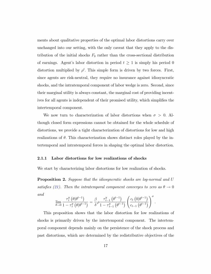
2.1.1 Labor distortions for low realizations of shocks

We start by characterizing labor distortions for low realization of shocks.

Proposition 2. Suppose that the idiosyncratic shocks are log-normal and U

satisfies (21). Then the intratemporal component converges to zero as θ → 0

and

limθ→0

τ yt(θ|θt−1

)1− τ yt

(θ|θt−1

) =β

δρ

τ yt−1

(θt−1

)1− τ yt−1

(θt−1

) ( ct (0|θt−1)

ct−1

(θt−1

))σ

.

This proposition shows that the labor distortion for low realizations of

shocks is primarily driven by the intertemporal component. The intertem-

poral component depends mainly on the persistence of the shock process and

past distortions, which are determined by the redistributive objectives of the

17

social planner and the history of idiosyncratic shocks accumulated by the agent

before period t. These observations also help explain the comparative statics

later in this section, for instance, with respect to the redistributive objective.

Before that, we show next that a different force shapes the labor distortion for

the high realizations of θt.

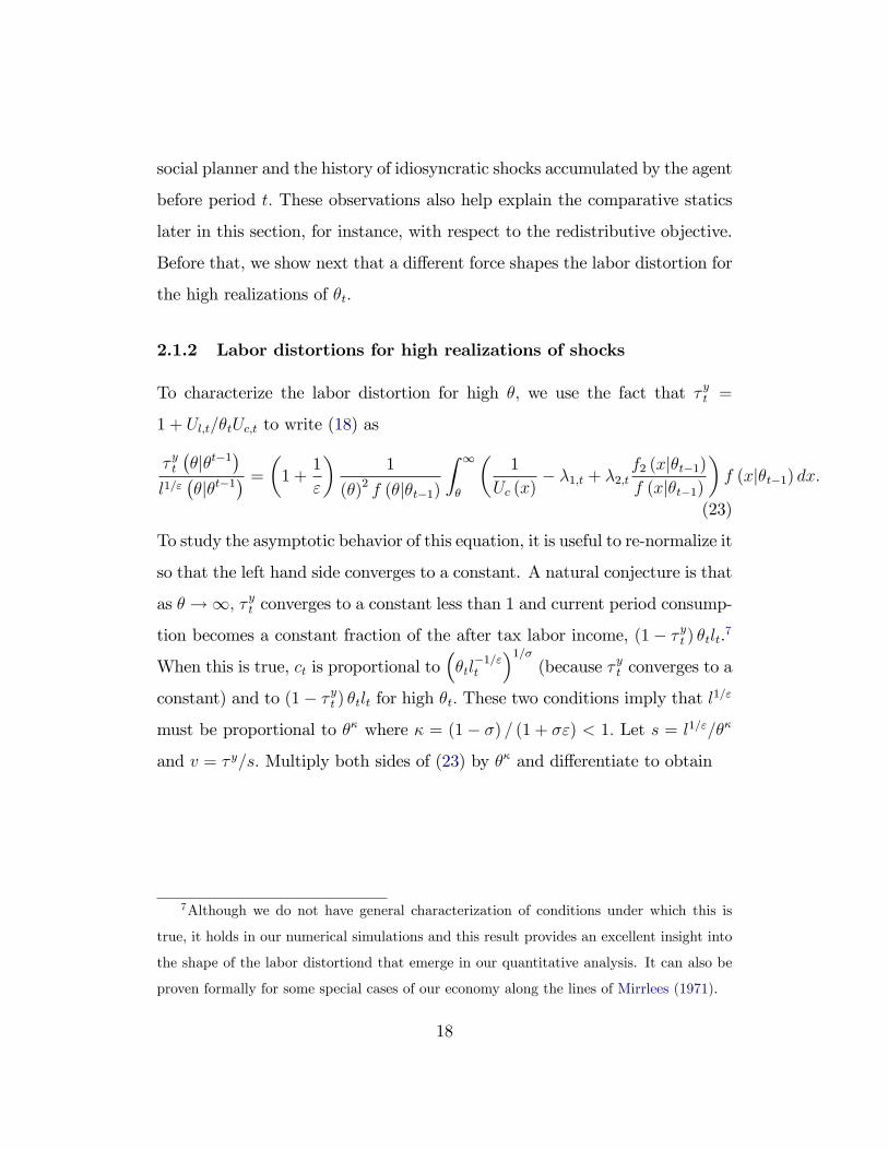
2.1.2 Labor distortions for high realizations of shocks

To characterize the labor distortion for high θ, we use the fact that τ yt =

1 + Ul,t/θtUc,t to write (18) as

τ yt(θ|θt−1

)l1/ε(θ|θt−1

) =

(1 +

1

ε

)1

(θ)2 f (θ|θt−1)

∫ ∞θ

(1

Uc (x)− λ1,t + λ2,t

f2 (x|θt−1)

f (x|θt−1)

)f (x|θt−1) dx.

(23)

To study the asymptotic behavior of this equation, it is useful to re-normalize it

so that the left hand side converges to a constant. A natural conjecture is that

as θ →∞, τ yt converges to a constant less than 1 and current period consump-

tion becomes a constant fraction of the after tax labor income, (1− τ yt ) θtlt.7

When this is true, ct is proportional to(θtl−1/εt

)1/σ

(because τ yt converges to a

constant) and to (1− τ yt ) θtlt for high θt. These two conditions imply that l1/ε

must be proportional to θκ where κ = (1− σ) / (1 + σε) < 1. Let s = l1/ε/θκ

and v = τ y/s. Multiply both sides of (23) by θκ and differentiate to obtain

7Although we do not have general characterization of conditions under which this is

true, it holds in our numerical simulations and this result provides an excellent insight into

the shape of the labor distortiond that emerge in our quantitative analysis. It can also be

proven formally for some special cases of our economy along the lines of Mirrlees (1971).

18

θdv

dθ= −

(1 +

1

ε

)(1

s− v − 1

θ1−κλ1,t

)− v

(2− κ+

θf ′

f

)︸ ︷︷ ︸

intratemporal component

(24)

−(

1 +1

ε

)λ2,t

1

θ1−κf2

f︸ ︷︷ ︸intertemporal component

,

where f ′ is a derivative of f (θ|θt−1) with respect to θ.

This equation allows one to study the effects of intra- and intertemporal

components on labor distortions for high realizations of shocks. When shocks

are log-normal, the intertemporal component converges to zero at the rate of1

θ1−κt

(see Lemma 2 in the online appendix for details). Thus, this term quickly

drops out from the law of motion for v.

The intratemporal component is much more slowly moving. Log-normality

implies that θf ′/f = − (ln θ − ρ ln θt−1) /σ2− 1.When θ is high and v is close

to its asymptotic values, dvd ln θ≈ 0, equation (24) implies that(

1 +1

ε

)(1

s− v)≈ −v

(1− κ−

(ln θ − ρ ln θt−1

σ2

)).

Since τ y = vs, it follows that

τ y (θ) ≈ (ε+ 1)[1 + εκ+

(ln θ−ρ ln θt−1

σ2

)ε] (25)

and

τ y (θ) ln θ →(

1 +1

ε

)σ2. (26)

This provides several insights. First, τ y converges to zero but at the rate of

ln θ. Since the rate of convergence of ln θ is very slow, in quantitative analyses

it will appear virtually flat when plotted against high values of θ. Second,

since the intertemporal component converges to zero at a much faster rate, the

19

50 100 150 2000

0.2

0.4

0.6

0.8

1

θ0

τy

C: Labor distortions in period 0

τy  staticτ0

y baseline

20 40 60 80 1000

0.2

0.4

0.6

0.8

1

θ1

τ 1yA: Labor distortions in period 1

τy1(θ1|θL)

τy1(θ

1|θ

H)

20 40 60 80 1000

0.2

0.4

0.6

0.8

1

θ1

τ 1y

B: Effects of variance of θ

σθ=0.55

σθ=0.70

σθ=0.85

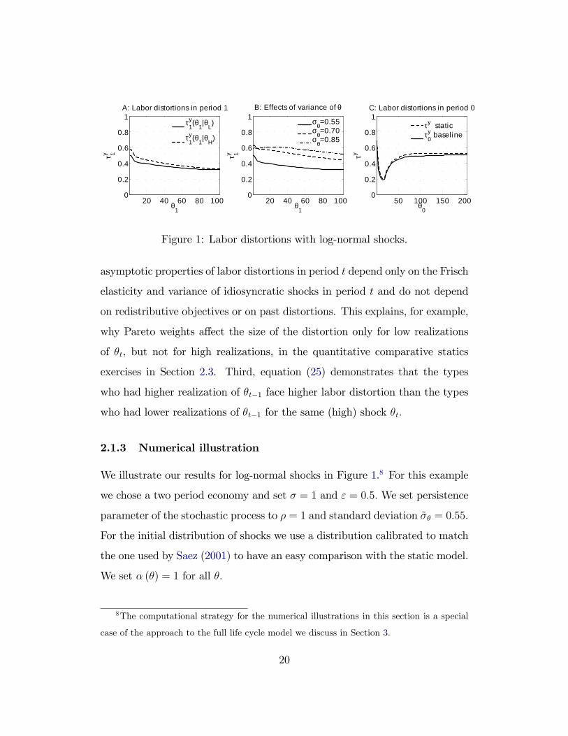
Figure 1: Labor distortions with log-normal shocks.

asymptotic properties of labor distortions in period t depend only on the Frisch

elasticity and variance of idiosyncratic shocks in period t and do not depend

on redistributive objectives or on past distortions. This explains, for example,

why Pareto weights affect the size of the distortion only for low realizations

of θt, but not for high realizations, in the quantitative comparative statics

exercises in Section 2.3. Third, equation (25) demonstrates that the types

who had higher realization of θt−1 face higher labor distortion than the types

who had lower realizations of θt−1 for the same (high) shock θt.

2.1.3 Numerical illustration

We illustrate our results for log-normal shocks in Figure 1.8 For this example

we chose a two period economy and set σ = 1 and ε = 0.5. We set persistence

parameter of the stochastic process to ρ = 1 and standard deviation σθ = 0.55.

For the initial distribution of shocks we use a distribution calibrated to match

the one used by Saez (2001) to have an easy comparison with the static model.

We set α (θ) = 1 for all θ.

8The computational strategy for the numerical illustrations in this section is a special

case of the approach to the full life cycle model we discuss in Section 3.

20

Panel A plots labor distortions in period 1 for two different realization of

θ in period 0, θH > θL. As our discussion of equation (25) explains, τy1 (·|θH)

is generally greater than τ y1 (·|θL) , and the difference between the two lines

shrinks for high θ. Panel B shows comparative statics of τ y1 (·|θH) for different

values of σθ. Following equations (25) and (26), higher variance of shocks leads

to higher distortions. Finally, Panel C shows the optimal labor distortions in

period 0 and compares them to the distortions that are obtained in the static

model. The two distortions are very similar. As we discuss in more details in

Section 2.3 and in Proposition 3, this result should generally be expected for

separable, isoelastic preferences.

An important feature of labor distortions with log-normal shocks is that

they appear essentially flat. We showed above that the intertemporal compon-

ent of the distortion starts at a positive value and decreases to zero relatively

rapidly, while the intratemporal component starts at zero, first increases and

then decreases very slowly. With log-normal shocks the decrease of the inter-

temporal component is being largely offset by the increase of the intratemporal

one, which leads to distortions that are essentially flat. This is one of the reas-

ons why the optimal linear distortions can approximate the optimum very well,

for example, in Farhi and Werning (2013).

2.2 Non-separable preferences

Previous section focused on separable, isoelastic preferences. That analysis

easily extends to other separable utility functions although some of the para-

meters will be endogenous. For example, when preferences take a form U (c, l) =

ln c + ln (1− l) , expression (26) still holds, but the Frisch elasticity of labor

supply depends on l and is equal to εθ = 1/ (1− l (θ)) .

21

The analysis may change significantly when consumption and labor are

complements. In this section, we focus on preferences with no income effect

popularized by Greenwood, Hercowitz and Huffman (1988), to which we refer

as GHH preferences:

U

(c−

(1 +

1

ε

)−1

l1+1/ε

). (27)

When U satisfies (27), 1 + 1εθ− γθ = 1 + 1

εand the expression (17) with

log-normal shocks becomes

τ yt(θ|θt−1

)1− τ yt

(θ|θt−1

) =

(1 +

1

ε

)1− F (θ|θt−1)

θf (θ|θt−1)(28)

×∫ ∞θ

exp

(∫ x

θ

βU ′′

U ′ω1 (x|x) dx

)(1− λ1,tU

′ (x))f (x|θt−1) dx

1− F (θ|θt−1)

+ρβ

δ

τ yt−1

(θt−1

)1− τ yt−1

(θt−1

) Uc (θ)

Uc(θt−1

) ∫∞θ exp(−∫ xθγx

dxx

)f2,t (x|θt−1) dx∫∞

θf2,t (x|θt−1) dx

,

where ω1 (θ|θ) = w (θ)− w2 (θ) .

Both intra- and intertemporal components of the labor distortion have

additional terms not present in the separable case. The intertemporal term

is multiplied by∫∞θ exp(−

∫ xθ γx

dxx )f2,t(x)dx∫∞

θ f2,t(x)dx. If θt > ρ ln θt−1, then f2 > 0 and

this term is less than one. The intratemporal component has an additional

term exp(∫ x

θβ U

′′

U ′ ω1 (x|x) dx). If Assumption 3 is satisfied, ω1 ≥ 0 and this

term is also less than one. Thus, non-separability introduces an additional

force that calls for lower distortions in dynamic economies, especially for high

types. The intuition for it is as follows. In a static economy the only way to

extract resources from high types is by taking a fraction of their labor income.

This distortion reduces agents’labor supply and, because of complementarily,

further increase their marginal utility of consumption, offsetting some gains. In

dynamic settings this can be avoided by extracting resources in future periods.

22

We illustrate this point in a simple two period economy when agents retire

in the second period. The advantage of this example is a simple closed form

expression for value function in period 1, V1 (w) , and in particular we know

that it is increasing in w. The arguments go through more generally for all

Vt (w,w2, θ) that have that property and we illustrate that in a stochastic

example that follows. We contrast the optimal distortions in GHH case with

those obtained with separable preferences.

Proposition 3. Suppose that T = 1 and FT (0|θ) = 1 for all θ.

1. Suppose U is of isoelastic form (21). Then τ y0 (θ) = τ ystatic (θ) where

τ ystatic (θ) is the optimal labor distortion in a static economy with the

same F0 and α.

2. Suppose U is of GHH form (27). If −U ′′/U ′ is bounded from below and

τ y0 is bounded away from 1, then limθ→∞ τy0 (θ) = 0.

The proof of this proposition is in the online appendix. In the proof we

also give suffi cient conditions on the primitives that ensure that τ y0 is bounded

away from 1 in part 2 of this Proposition.

This proposition highlights important differences in the intertemporal pro-

vision of incentives with and without complementaries. With separable, isoelastic

preferences the optimal labor distortion in period 0 is not affected by retire-

ment period and coincides with static optimal distortions. With non-separable

GHH preferences (at least when −U ′′/U ′ is bounded) it is optimal not to dis-

tort labor supply of high types, and, unlike in a static economy, this result does

not depend on the distribution F0. This stark result follows from our discus-

sion of the role of complementarities in equation (28). With GHH preferences

γ = −U ′′/U ′l1+1/ε and this term goes to infinity for high types when −U ′′/U ′

23

50 100 150 2000

0.2

0.4

0.6

0.8

1

θ0

τ 0yA: Labor distortions in period 0

CESLog GHHExp GHH

20 40 60 80 1000

0.2

0.4

0.6

0.8

1

θ1

τ 1y

C: Labor distortions in period 1

CESLog GHHExp GHH

50 100 150 2000

0.2

0.4

0.6

0.8

1

θ0

τ 0s

B: Savings distortions

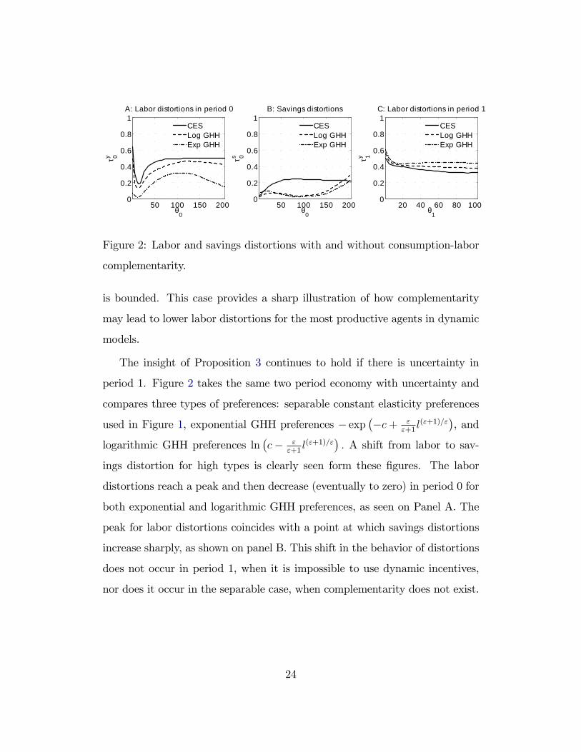
CESLog GHHExp GHH

Figure 2: Labor and savings distortions with and without consumption-labor

complementarity.

is bounded. This case provides a sharp illustration of how complementarity

may lead to lower labor distortions for the most productive agents in dynamic

models.

The insight of Proposition 3 continues to hold if there is uncertainty in

period 1. Figure 2 takes the same two period economy with uncertainty and

compares three types of preferences: separable constant elasticity preferences

used in Figure 1, exponential GHH preferences − exp(−c+ ε

ε+1l(ε+1)/ε

), and

logarithmic GHH preferences ln(c− ε

ε+1l(ε+1)/ε

). A shift from labor to sav-

ings distortion for high types is clearly seen form these figures. The labor

distortions reach a peak and then decrease (eventually to zero) in period 0 for

both exponential and logarithmic GHH preferences, as seen on Panel A. The

peak for labor distortions coincides with a point at which savings distortions

increase sharply, as shown on panel B. This shift in the behavior of distortions

does not occur in period 1, when it is impossible to use dynamic incentives,

nor does it occur in the separable case, when complementarity does not exist.

24

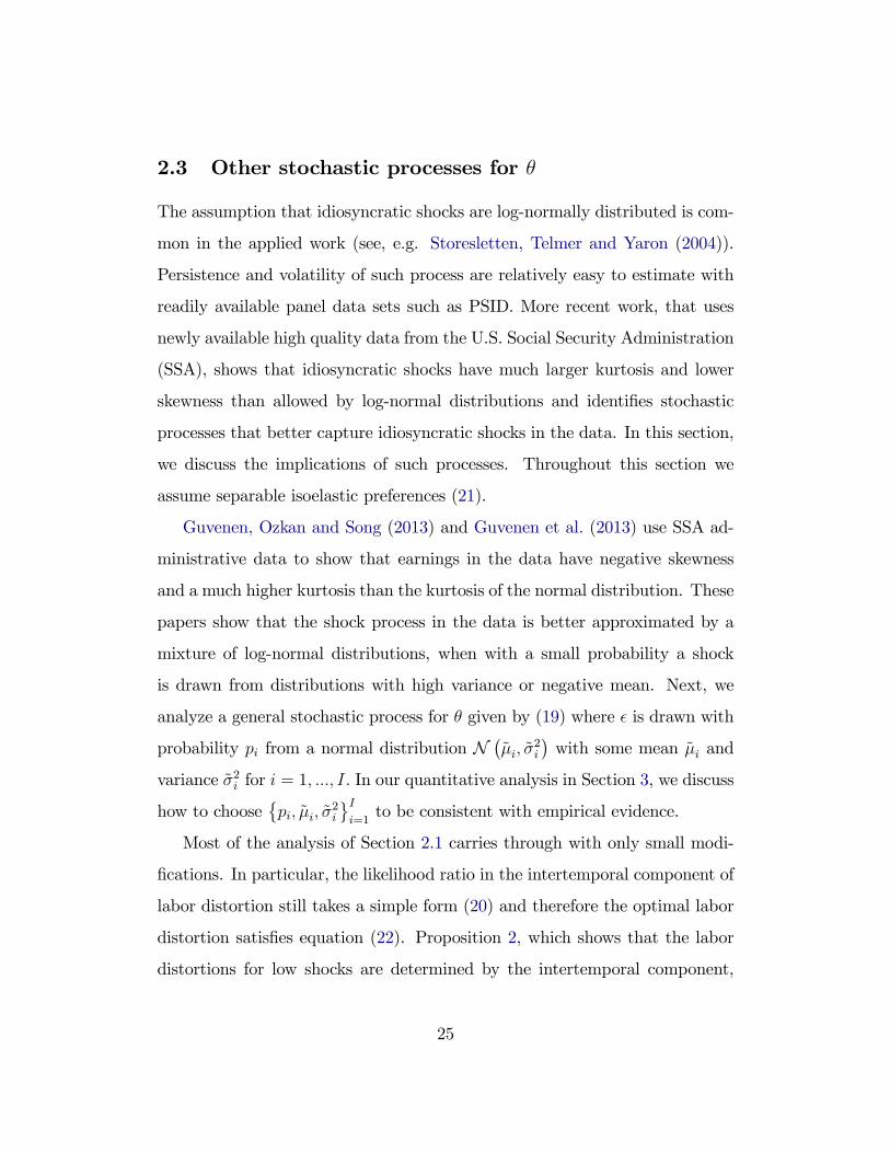
2.3 Other stochastic processes for θ

The assumption that idiosyncratic shocks are log-normally distributed is com-

mon in the applied work (see, e.g. Storesletten, Telmer and Yaron (2004)).

Persistence and volatility of such process are relatively easy to estimate with

readily available panel data sets such as PSID. More recent work, that uses

newly available high quality data from the U.S. Social Security Administration

(SSA), shows that idiosyncratic shocks have much larger kurtosis and lower

skewness than allowed by log-normal distributions and identifies stochastic

processes that better capture idiosyncratic shocks in the data. In this section,

we discuss the implications of such processes. Throughout this section we

assume separable isoelastic preferences (21).

Guvenen, Ozkan and Song (2013) and Guvenen et al. (2013) use SSA ad-

ministrative data to show that earnings in the data have negative skewness

and a much higher kurtosis than the kurtosis of the normal distribution. These

papers show that the shock process in the data is better approximated by a

mixture of log-normal distributions, when with a small probability a shock

is drawn from distributions with high variance or negative mean. Next, we

analyze a general stochastic process for θ given by (19) where ε is drawn with

probability pi from a normal distribution N(µi, σ

2i

)with some mean µi and

variance σ2i for i = 1, ..., I. In our quantitative analysis in Section 3, we discuss

how to choose{pi, µi, σ

2i

}Ii=1

to be consistent with empirical evidence.

Most of the analysis of Section 2.1 carries through with only small modi-

fications. In particular, the likelihood ratio in the intertemporal component of

labor distortion still takes a simple form (20) and therefore the optimal labor

distortion satisfies equation (22). Proposition 2, which shows that the labor

distortions for low shocks are determined by the intertemporal component,

25

also extends to this case. The proof of this Proposition used the fact that for

log-normal density function limθ→0 θf′/f = ∞. The same property continues

to hold for a mixture of log-normals9 and hence Proposition 2 and discussion

in Section 2.1.1 are valid for the more general shock process.

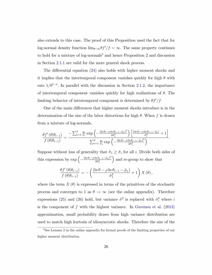
The differential equation (24) also holds with higher moment shocks and

it implies that the intertemporal component vanishes quickly for high θ with

rate 1/θ1−κ. In parallel with the discussion in Section 2.1.2, the importance

of intertemporal component vanishes quickly for high realizations of θ. The

limiting behavior of intratemporal component is determined by θf ′/f.

One of the main differences that higher moment shocks introduce is in the

determination of the size of the labor distortions for high θ. When f is drawn

from a mixture of log-normals,

θf ′ (θ|θt−1)

f (θ|θt−1)=−∑I

i=1piσi

exp(− (ln θt−ρ ln θt−1−µi)2

2σ2i

) [(ln θt−ρ ln θt−1−µi)

σ2i

+ 1]

∑Ii=1

piσi

exp(− (ln θt−ρ ln θt−1−µi)2

2σ2i

) .

Suppose without loss of generality that σ1 ≥ σi for all i. Divide both sides of

this expression by exp(− (ln θt−ρ ln θt−1−µ1)2

2σ21

)and re-group to show that

θf ′ (θ|θt−1)

f (θ|θt−1)= −

((ln θ − ρ ln θt−1 − µ1)

σ21

+ 1

)X (θ) ,

where the term X (θ) is expressed in terms of the primitives of the stochastic

process and converges to 1 as θ → ∞ (see the online appendix). Therefore

expressions (25) and (26) hold, but variance σ2 is replaced with σ2i where i

is the component of f with the highest variance. In Guvenen et al. (2013)

approximation, small probability draws from high variance distribution are

used to match high kurtosis of idiosyncratic shocks. Therefore the size of the

9See Lemma 2 in the online appendix for formal proofs of the limiting properties of our

higher moment distribution.

26

20 40 60 80 1000

0.2

0.4

0.6

0.8

1

θ1

τ 1yA: Higher moments and τy

1

kurtosis=20kurtosis=12log­normal

20 40 60 80 1000

0.2

0.4

0.6

0.8

1

θ0

τ 0s

B: Higher moments and τs0

kurtosis=20kurtosis=12log­normal

20 40 60 80 1000

0.2

0.4

0.6

0.8

1

θ1

τ 1y

C: Redistribution and τy1

a=0a=5a=10

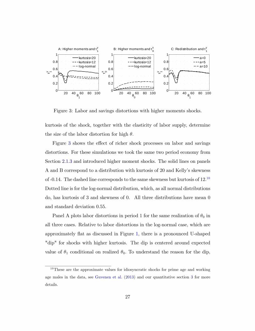
Figure 3: Labor and savings distortions with higher moments shocks.

kurtosis of the shock, together with the elasticity of labor supply, determine

the size of the labor distortion for high θ.

Figure 3 shows the effect of richer shock processes on labor and savings

distortions. For these simulations we took the same two period economy from

Section 2.1.3 and introduced higher moment shocks. The solid lines on panels

A and B correspond to a distribution with kurtosis of 20 and Kelly’s skewness

of -0.14. The dashed line corresponds to the same skewness but kurtosis of 12.10

Dotted line is for the log-normal distribution, which, as all normal distributions

do, has kurtosis of 3 and skewness of 0. All three distributions have mean 0

and standard deviation 0.55.

Panel A plots labor distortions in period 1 for the same realization of θ0 in

all three cases. Relative to labor distortions in the log-normal case, which are

approximately flat as discussed in Figure 1, there is a pronounced U-shaped

"dip" for shocks with higher kurtosis. The dip is centered around expected

value of θ1 conditional on realized θ0. To understand the reason for the dip,

10These are the approximate values for idiosyncratic shocks for prime age and working

age males in the data, see Guvenen et al. (2013) and our quantitative section 3 for more

details.

27

note from formula (22) that the labor distortion for type θ depends on the tail

ratio term (1− F (θ|θ0)) /θf (θ|θ0) . High kurtosis distributions have higher

mass around E [θ|θ0] , which lowers this tail ratio. At the same time the labor

distortions for high realizations of θ1 are higher than for log-normal which is

driven by the fact that the size of those distortions are driven by the magnitude

of the kurtosis as discussed above.

Panel B compares savings distortions τ s0 (θ0) . Even though the first and the

second moments are the same in all three distributions, large kurtosis leads to

smaller distortions. More disperse distribution of shocks makes provision of

insurance more important, which lowers the savings wedge implied by Jensen’s

inequality and the Inverse Euler Equation.

Panel C plots labor wedges in period 1 for different redistributive object-

ives. We assume that Pareto weights are α (θ) ∝ θ−a and plot τ y1 (·|θ0) given

the same θ0 but different values of a. The more redistributive (higher a) the

social planner is, the higher the labor distortions is for low realizations of θ,

but not for the high ones. This result can be understood from our discussion of

the relative importance of intra- and inter-temporal components for different

shocks. Labor distortions for low shocks are driven by the intertemporal com-

ponents, which carries over the distortions inherited from previous periods.

More redistributive planner sets higher labor distortions in period 0, which

leads to higher distortions for low realizations of θ1. On the other hand, the

labor distortions for high realizations of θ1 are driven by the intratemporal

component, which depends only on kurtosis and the elasticity of labor supply

in the right tail. One of the implications of this observation is that the size

and shape of labor distortions for high θ are independent of the redistributive

objectives of the government; they are driven purely by the insurance needs

of the agent.

28

While a mixture of log-normal distributions captures well idiosyncratic

shocks experienced by individuals over lifetime, it fails to produce fat-tailed

cross-sectional distribution observed in the data. To capture such tails, one

can assume that the initial types are drawn from a distribution F0 which has a

Pareto tail with some coeffi cient a. This assumption introduces only minimal

changes to our discussion of labor distortions for high shocks in Section 2.1.2.

Suppose that α (x) is non-increasing. The differential equation (24) still holds

but Pareto tails imply that θ0f′0/f0 → −a− 1. Taking the limits, the optimal

labor distortion satisfies

limθ→∞

τ y (θ) =1 + ε

1 + ε (κ+ a)=

11

1+εσ+ a ε

1+ε

. (29)

When shocks have Pareto tails, labor distortions converge to a positive number

which depends only on Frisch elasticity ε and σ as well as the thickness of the

tail a.

This formula is closely related to the closed form expression for optimal

taxes obtained by Saez (2001) in static models. Saez (2001, equation (9))

showed that if empirical cross-sectional distribution of earning θl is Pareto with

tail a, and ζu and ζc are uncompensated and compensated elasticities of labor

supply, then τ y → 1/ (1 + ζu + ζc (a− 1)) as θ → ∞. Since the relationship

between the tail of θ, a, and the tail of θl, a, is given by a = (1 + ζu) a,11 this

can be re-written as

τ → 1

1 + ζu − ζc + aζc

1+ζu

. (30)

When preferences take the form (21), ζu → ε 1−σ1+εσ

and ζc → ε1+εσ

as θ → ∞.

Substituting that into (30) and re-arranging we obtain (29).

11This follows from Lemma 1 in Saez (2001) that shows that dyy = (1 + ζu) dθθ .

29

3 Quantitative analysis

We now turn to the quantitative study of a calibrated life cycle model. We

chose a 50 period economy in which agents work for the first 40 years and then

retire for the last 10 years. Agents’utility function is

ln c−(

1 +1

ε

)−1

l1+1/ε

with ε = 0.5. We set β = δ = 0.95 and chose utilitarian Pareto weights.

Stochastic process for skills. Our theoretical analysis unambiguously points

to the stochastic process for idiosyncratic shocks, and especially its higher mo-

ments, as a crucial input for a quantitative analysis. We rely on the findings

of the recent work by Guvenen, Ozkan and Song (2013) and Guvenen et al.

(2013), who use a newly available high quality administrative data from the

U.S. Social Security Administration based on a random sample of 10% U.S.

taxpayers. For our purposes their approach has significant advantages over

using easily accessible panel data sets such as U.S. Panel Study of Income

Dynamics (PSID). The small sample size and top coding in those data sets

do not allow to estimate higher moments well and, consequently, researchers

often assume a log-normal shock process (e.g. Storesletten, Telmer and Yaron

(2004)).12

Guvenen et al. (2013) find that the persistence of annual log earning for

working age males is close to one and its standard deviation is about 0.55.

12In the previous version of the paper (Golosov, Troshkin and Tsyvinski (2011)) we used

PSID together with the TAXSIM’s calculations of individuals’effective marginal tax rates

to estimate non-parametrically stochastic process for θt. Our estimated stochastic process

was close to log-normal but a small number of observations in the tails and top coding made

a good estimation of higher moments impossible.

30

Higher moments are significantly different from those implies by a log-normal

distribution. In particular, the kurtosis of the shocks to log earning for prime

age males (35 to 55 years old) is about 20, while kurtosis for all working

age makes (25 to 60 years old) is about 12. Kelly’s skewness, defined as(P90−P50)−(P50−P10)

(P90−P10), where Pz is the zth percentile growth rate, is about −0.14

for both prime age and working age males. Guvenen, Ozkan and Song (2013)

and Guvenen et al. (2013) also show that the empirical shock process can

be approximated well by a mixture of three log-normal distributions, shocks

from two of which are drawn with low probabilities. The high probability

distribution controls the variance of the shocks while the two low probability

distributions control its kurtosis and skewness.

Guvenen et al. (2013) report these statistics for the stochastic process for

earnings, not skills θ or wages. In principle, one can structurally estimate θ

by using observations for earnings and taxes. This would require access to the

restricted SSA data and would be far beyond the scope of this paper. Instead

we chose a simpler route. Our preferences imply that log earning of individuals

who have a small amount of assets and transfers should follow approximately

the same process as log θ. Thus we chose stochastic process for θ to match

the moments reported by Guvenen et al. (2013). We believe the benefits of

transparency of this approach outweigh possible costs.

We assume that the stochastic process for θt follows

ln θt = ln θt−1 + εt,

where

εt =

ε1,t ∼ N (µ1, σ1) w.p. p1

ε2,t ∼ N (µ2, σ2) w.p. p2

ε3,t ∼ N (µ3, σ3) w.p. p3

31

Table 1: Parametrization of the stochastic process

µ1 µ2 µ3 σ1 σ2 σ3 p1 p2 p3

0.05 0 -0.4 0.19 1.6 0.16 0.8 0.1 0.1

and {µi, σi, pi}3i=1 are chosen to match the annual values of standard devi-

ation of 0.55, kurtosis of 20 and Kelly’s skewness of −0.14 for εt. The exact

parameters are given in Table 1.

Finally, we need to choose distribution F0 (θ) from which agents draw their

shocks in period 0. Ideally, one would infer it from observations of wages or

earnings early in life, e.g., for the 25 to 30 year old. Such data are available

but access to it is restricted. Instead, we use F0 (θ) to match cross-sectional

distribution reported by Saez (2001).13 This makes our distortions in period

0 directly comparable to his. As we discussed in the theoretical part of the

paper, this approach overpredicts the true size of initial heterogeneity and

overestimates the size of the optimal period 0 labor distortions, as well as

labor distortions for low realizations of θt in subsequent periods. Initial dis-

tribution, however, does not affect the shape or the size of the distortions for

high realizations of θt.

Computational strategy. We rely on the recursive structure of the dual

formulation of the planner’s problem, that we explored in the theoretical ana-

lysis, to solve numerically the problem of this size and complexity (i.e., with

multitude of periods and correlated shocks). We provide a summary of our

13Analogous to the calibration procedure for the stochastic process for the shocks above,

we mix a log-normal distribution with a Pareto tail to match Figure 4 in Saez (2001). We

set Pareto tail parameter a = 2 and start the tail at θ corresponding to income of $150,000

per year following Figure 2 and its discussion in Saez (2001).

32

computational approach here while the online appendix contains additional

details.

Our main problem is a finite-horizon discrete-time dynamic programming

problem with a three-dimensional continuous state space. First, we implement

a value function iteration algorithm. We start from period T−1 and proceed by

backward induction. The last working period, T−1, incorporates present value

of resources needed to provide promised utility over the remaining T − T + 1

retirement periods. Before proceeding to a previous period, we approximate

value functions with tensor products of orthogonal polynomials evaluated at

their root nodes. To solve each node’s minimization sub-problem effi ciently, we

use an implementation of interior-point algorithm, with a trust-region method

to solve barrier problems and an l1 barrier penalty function. We verify that

increasing properties in Assumption 3 are satisfied numerically. Assumptions

1 and 2 are satisfied trivially for the preferences and parameter values we chose

above. Next, we compute w0 such that V0 (w0) = 0. Given continuously differ-

entiable approximation of V0, we solve for w0 by binary jumps and bisection.

We compute optimal allocations reported below by forward induction starting

with the policies given by V0 (w0) = 0. Optimal labor and savings distortions

are then computed from the policy functions using definitions (14) and (15).

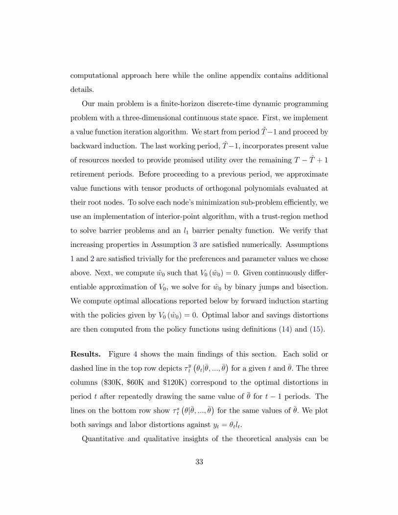
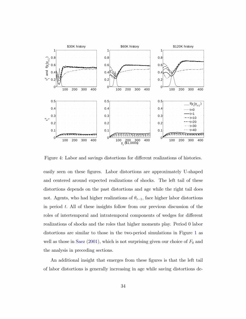
Results. Figure 4 shows the main findings of this section. Each solid or

dashed line in the top row depicts τ yt(θt|θ, ..., θ

)for a given t and θ. The three

columns ($30K, $60K and $120K) correspond to the optimal distortions in

period t after repeatedly drawing the same value of θ for t − 1 periods. The

lines on the bottom row show τ st(θ|θ, ..., θ

)for the same values of θ. We plot

both savings and labor distortions against yt = θtlt.

Quantitative and qualitative insights of the theoretical analysis can be

33

100 200 300 4000

0.2

0.4

0.6

0.8

1τ ty   a

nd  f

(yt|y

t­1)

$30K history

100 200 300 4000

0.1

0.2

0.3

0.4

0.5

τ ts

100 200 300 4000

0.2

0.4

0.6

0.8

1$60K history

100 200 300 4000

0.1

0.2

0.3

0.4

0.5

yt ($1,000s)

100 200 300 4000

0.2

0.4

0.6

0.8

1$120K history

100 200 300 4000

0.1

0.2

0.3

0.4

0.5f(y

t|y

t­1)

t=0t=1t=10t=20t=30t=40

Figure 4: Labor and savings distortions for different realizations of histories.

easily seen on these figures. Labor distortions are approximately U-shaped

and centered around expected realizations of shocks. The left tail of these

distortions depends on the past distortions and age while the right tail does

not. Agents, who had higher realizations of θt−1, face higher labor distortions

in period t. All of these insights follow from our previous discussion of the

roles of intertemporal and intratemporal components of wedges for different

realizations of shocks and the roles that higher moments play. Period 0 labor

distortions are similar to those in the two-period simulations in Figure 1 as

well as those in Saez (2001), which is not surprising given our choice of F0 and

the analysis in preceding sections.

An additional insight that emerges from these figures is that the left tail

of labor distortions is generally increasing in age while saving distortions de-

34

crease.14 The observation is driven by the fact that variance of consumption

decreases as retirement approaches, the forces discovered by Farhi andWerning

(2013) when the shocks are log-normal. Our figures show that the increase in

the optimal labor distortions is asymmetric. Only the left tail of the distortions

increases, the effect that can be seen from Proposition 2, since lower variance of

consumption also means that consumption growth term ct(0|θt−1

)/ct−1

(θt−1

)is bigger. The right tail of the distortions does not change with age since it

is pinned down by kurtosis and the elasticity of labor supply and does not

depend on other parameters, such as age.

4 Conclusion

In this paper we take a step toward characterization of optimal labor and

savings distortions in a life cycle model. These distortions are driven by an

interplay of redistributive objectives and the need to provide insurance against

idiosyncratic shocks. We show how the size of the distortions depends on the

parameters that can be measured directly in the data. Our analysis unambigu-

ously points to the importance of higher moments of the idiosyncratic shock

process that the individuals face, and in particular its kurtosis.

For our life cycle calibration we chose what we viewed to be the simplest

and most transparent strategy. The estimation of the underlying stochastic

processes can be further refined to produce better estimates of the distortions.

We also did not discuss the role of heterogeneity in shock process among rich

14The fact that savings distortions decrease with age is sensitive to the assumption that

there is no complementarity between consumption and labor. When labor and consumption

are complements, the savings distortion may increase with age, as with, for example, GHH

preferences (see Golosov, Troshkin and Tsyvinski (2011)).

35

and poor agents. Such heterogeneity is present in the data (see Guvenen,

Ozkan and Song (2013)) and we leave the investigation of its role to future

work.

Our analysis focuses on the distortions in fully optimal allocations which

are restricted only by informational constraint. Implementations of these al-

locations may require complex history dependence in a tax code. We view

our approach as complementary to, e.g., the one taken by Conesa, Kitao and

Krueger (2009). They study tax reforms and the optimal taxes within a set of

the parametrically restricted tax functions. One advantage of that approach

over solving for the full informationally constrained optimum is that it focuses

on simpler taxes. Our paper points out the elements that may be important

in choosing the parameters of such tax functions.

References

Abraham, Arpad, and Nicola Pavoni. 2008. “Effi cient Allocations with

Moral Hazard and Hidden Borrowing and Lending: A Recursive Formula-

tion.”Review of Economic Dynamics, 11(4): 781—803.

Albanesi, Stefania, and Christopher Sleet. 2006. “Dynamic Optimal

Taxation with Private Information.”Review of Economic Studies, 73(1): 1—

30.

Ales, Laurence, and Pricila Maziero. 2007. “Accounting for Private In-

formation.”working paper.

Browning, Martin, Lars Peter Hansen, and James J. Heckman. 1999.

“Micro Data and General Equilibrium Models.”In Handbook of Macroeco-

36

nomics. Vol. 1 of Handbook of Macroeconomics, , ed. J. B. Taylor and M.

Woodford, Chapter 8, 543—633. Elsevier.

Conesa, Juan Carlos, Sagiri Kitao, and Dirk Krueger. 2009. “Taxing

Capital? Not a Bad Idea After All!”American Economic Review, 99(1): 25—

48.

Diamond, Peter. 1998. “Optimal Income Taxation: An Example with a

U-Shaped Pattern of Optimal Marginal Tax Rates.”American Economic

Review, 88(1): 83—95.

Farhi, Emmanuel, and IvánWerning. 2013. “Insurance and Taxation over

the Life Cycle.”Review of Economic Studies, 80(2): 596—635.

Fernandes, Ana, and Christopher Phelan. 2000. “A Recursive Formula-

tion for Repeated Agency with History Dependence.”Journal of Economic

Theory, 91(2): 223—247.

Fukushima, Kenichi. 2010. “Quantifying the Welfare Gains from Flexible

Dynamic Income Tax Systems.”mimeo.

Golosov, Mikhail, Aleh Tsyvinski, and Iván Werning. 2006. “New

Dynamic Public Finance: A User’s Guide.”NBER Macroeconomics Annual,

21: 317—363.

Golosov, Mikhail, Aleh Tsyvinski, and Nicolas Werquin. 2013. “Dy-

namic Tax Reforms.”working paper.

Golosov, Mikhail, and Aleh Tsyvinski. 2006. “Designing Optimal Disab-

ility Insurance: A Case for Asset Testing.” Journal of Political Economy,

114(2): 257—279.

37

Golosov, Mikhail, Maxim Troshkin, and Aleh Tsyvinski. 2011. “Op-

timal Dynamic Taxes.”NBER Working Paper 17642.

Golosov, Mikhail, Narayana Kocherlakota, and Aleh Tsyvinski. 2003.

“Optimal Indirect and Capital Taxation.” Review of Economic Studies,

70(3): 569—587.

Greenwood, Jeremy, Zvi Hercowitz, and Gregory W Huffman. 1988.

“Investment, Capacity Utilization, and the Real Business Cycle.”American

Economic Review, 78(3): 402—17.

Grochulski, Borys, and Narayana Kocherlakota. 2010. “Nonseparable

Preferences and Optimal Social Security Systems.” Journal of Economic

Theory, 145: 2055—77.

Guvenen, Fatih, Fatih Karahan, Serdar Ozkan, and Jae Song. 2013.

“What Do Data onMillions of U.S. Workers Say About Labor Income Risk?”

Working paper.

Guvenen, Fatih, Serdar Ozkan, and Jae Song. 2013. “The Nature of

Countercyclical Income Risk.”Working paper.

Judd, Kenneth L. 1998. Numerical Methods in Economics. The MIT Press.

Judd, Kenneth L., and Che-Lin Su. 2006. “Optimal Income Taxation

with Multidimensional Taxpayer Types.”working paper.

Kapicka, Marek. 2013. “Effi cient Allocations in Dynamic Private Informa-

tion Economies with Persistent Shocks: A First-Order Approach.”Review

of Economic Studies, 80(3): 1027—1054.

38

Kocherlakota, Narayana. 2005. “Zero Expected Wealth Taxes: A Mirrlees

Approach to Dynamic Optimal Taxation.”Econometrica, 73(5): 1587—1621.

Kocherlakota, Narayana. 2010. The New Dynamic Public Finance. Prin-

ceton University Press, USA.

Mirrlees, James. 1971. “An Exploration in the Theory of Optimum Income

Taxation.”Review of Economic Studies, 38(2): 175—208.

Mirrlees, James. 1976. “Optimal Tax Theory: A Synthesis.” Journal of

Public Economics, 6(4): 327—358.

Pavan, Alessandro, Ilya Segal, and Juuso Toikka. 2010. “Dynamic

Mechanism Design: Incentive Compatibility, Profit Maximization and In-

formation Disclosure.”working paper.

Saez, Emmanuel. 2001. “Using Elasticities to Derive Optimal Income Tax

Rates.”Review of Economic Studies, 68(1): 205—229.

Storesletten, Kjetil, Christopher I. Telmer, and Amir Yaron. 2004.

“Cyclical Dynamics in Idiosyncratic Labor Market Risk.”Journal of Polit-

ical Economy, 112(3): 695—717.

Su, Che-Lin., and Kenneth L. Judd. 2007. “Computation of Moral-

Hazard Problems.”working paper.

Tuomala, Matti. 1990. Optimal Income Tax and Redistribution. Oxford Uni-

versity Press, USA.

Weinzierl, Matthew. 2011. “The Surprising Power of Age-Dependent

Taxes.”Review of Economic Studies, 78(4): 1490—1518.

39

Werning, Iván. 2009. “Nonlinear Capital Taxation.”MIT working paper.

Wilson, R. 1996. “Nonlinear Pricing and Mechanism Design.”Handbook of

Computational Economics, 1: 253—293.

40

A Online Appendix

A.1 Proof of Lemma 1

Note that given any solution u∗ (θ) following a sequence of reports(θt−1, θ

),

we can construct

ω(θ|θ)

=

∫ ∞0

u∗(θt−1, θ, s

)ft+1 (s|θ) ds.

We can re-write (6) as

maxθV(θ; θ)≡ max

θU(c(θ), y(θ); θ

)+ βω(θ|θ).

Since c (·) and ω (·|θ) are piecewise C1, they are differentiable except at a

finite number of points. Then for all θ where it is differentiable,

Uc (c(θ), y(θ); θ) c′ (θ) + Uy (c(θ), y(θ); θ) y′ (θ) + βω1(θ|θ) = 0, (31)

where c′ and y′ are derivatives of c and y. Optimality requires that y (·) and

V (·; θ) are piecewise C1 and if c (·) and ω (·|θ) are.

Suppose that the global incentive constraint is violated, i.e. V(θ; θ)−

V (θ; θ) > 0 for some θ. Suppose θ > θ is a point of differentiability. Then

0 <

∫ θ

θ

∂V (x; θ)

∂xdx

=

∫ θ

θ

[Uc (x; θ)

dc

dx+ Uy (x; θ)

dy

dx+ β

dω (x|θ)dx

]dx.

Since all the objects in the integral are piecewise differentiable, it can be

represented as a finite sum of the terms∫ θj+1

θj

Uc (x; θ)

[c′ (x) + y′ (x)

Uy (x; θ)

Uc (x; θ)+ β

ω1 (x|θ)Uc (x; θ)

]dx

for some finite number of intervals (θj, θj+1) .

i

If x > θ, Uy(x;θ)

Uc(x;θ)≤ Uy(x;x)

Uc(x;x)and Uc (x; θ) ≥ Uc (x;x) (from the single crossing

property and complementarity in Assumption 1 respectively) and ω1 (x|x) ≥

ω1 (x|θ) from Assumption 3. Therefore∫ θj+1

θj

Uc (x; θ)

[c′ (x) + y′ (x)

Uy (x; θ)

Uc (x; θ)+ β

ω1 (x|θ)Uc (x; θ)

]dx

≤∫ θj+1

θj

Uc (x; θ)

[c′ (x) + y′ (x)

Uy (x;x)

Uc (x;x)+ β

ω1 (x|x)

Uc (x;x)

]dx

= 0

where the last equality follows from (31). Therefore,∫ θθ∂V(x;θ)∂x

dx ≤ 0, a con-

tradiction. If θ < θ the arguments are analogous. Finally, since V(θ; θ)is

continuous in θ, taking limits establishes that V(θ; θ)≤ V (θ; θ) at the points

of non-differentiability.

A.2 Details of Section 2

We drop explicit time subscripts t whenever it does not lead to confusion. The

Hamiltonian to problem (7) is

H = (c− θl + δVt+1 (w,w2, θ)) ft + µ

[−Ul(c, l)

l

θ+ βw2

]−λ1u (θ) ft + λ2u (θ) f2,t + ϕ [u− U(c, l)− βw]

and the envelope conditions are

∂Vt∂w

= λ1,∂Vt∂w2

= −λ2. (32)

The first order conditions are

[u] : ϕ− λ1f + λ2f2 = −µ

[l] : −Ulϕ− θf = −1θµ[Ulll+UlUl

](−Ul)

[c] : f − µUcl lθ = ϕUc

ii

[w] : δ ∂Vt+1

∂wf = ϕβ

[w2] : δ ∂Vt+1

∂w2f = −µβ

Use the first order condition for c to substitute away for ϕ

[u] : 1Ucf − λ1f + λ2f2 − µ

θUcllUc

= −µ

[l] : −UlUcf − µUcll

Uc

(−Ul)θ− θf = −1

θµ[Ulll+UlUl

](−Ul)

[w] : δβ∂Vt+1

∂w= 1

Uc− µ

θfUcllUc

[w2] : δβ∂Vt+1

∂w2= −µ

f

Use definitions of εθ, γθto write the first order condition for l as(UlθUc

+ 1

)θf =

1

θµ

(1 +

1

εθ− γθ

)(−Ul)

Since τ y = 1 + UlθUc

this can be equivalently written as

τ y

1− τ y =µUcθf

(1 +

1

εθ− γθ

). (33)

This expression together with [w2] implies

λ2,t+1 = −∂Vt+1

∂w2

=β

δ

τ yθt1− τ yθt

θtUc (θt)

(1 +

1

εθt− γθt

)−1

. (34)

To find µ we integrate [u]

µ (θ) =

∫ ∞θ

exp

(−∫ x

θ

γxdx

x

)(1

Uc (x)f (x)− λ1f (x) + λ2f2 (x)

)dx

From boundary condition µ (0) = 0 we get

λ1,t =

∫∞0

exp(−∫ x

0γx

dxx

) (1Ucft + λ2,tf2,t

)dx∫∞

0exp

(−∫ x

0γx

dxx

)ftdx

(35)

and λ2,t is given by (34).

Use the expression for µ (θ) and (34) for t− 1 to substitute into (33)

τ y (θ)

1− τ y (θ)=

(1 +

1

εθ− γθ

)1

θtft (θ)

∫ ∞θ

Uc (θt)

Uc (x)exp

(−∫ x

θ

γxdx

x

)(1− λ1,tUc (x)) ft (x) dx

+β

δ

τ yθt−1

1− τ yθt−1

1 + 1εθ− γθ

1 + 1εθt−1

− γθt−1

Uc (θ)

Uc(θt−1

) θt−1

θft (θ)

∫ ∞θ

exp

(−∫ x

θ

γxdx

x

)f2,t (x) dx

iii

which is the same expression as (17). This proof with slight modifications also

yields (18).

Period 0 expression and static expression can be derived along the same

lines. In both cases λ2,0 = 0 and the condition for [u] is replaced by the

expression ϕ− λ1αf = −µ. The rest of the analysis is unchanged.

Finally, we prove Proposition 1. Note that we can express ϕ using the first

order conditions for w rather than c in which case the differential equation for

µ becomes δβ∂Vt+1

∂wf − λ1f + λ2f2 = −µ. Integrate this expression from 0 to

infinity, use the boundary conditions µ (0) = µ (∞) = 0 and∫∞

0f2dx = 0 to

obtain15

λ1,t =δ

β

∫ ∞0

∂Vt+1

∂w(x) f (x) dx.

Combine this expression with (32) to get ∂Vt∂w

= δβEt ∂Vt+1

∂wand by the law of

iterated expectations∂Vt∂w

=

(δ

β

)T−t−1

Et∂VT∂w

.

When FT (0|θ) = 1 for all θ, ∂VT∂w

(θT)

= 1

Uc(θT ), which, in combination with

the first order condition on [w] implies

1

Uc(θt) − µ

θfγθ =

(δ

β

)T−tEt

1

Uc(θT)

From Assumption 2 1 + 1εθ− γθ > 0, and then from equation (33) the sign

of µ is equal to the sign of τ y. Thus if τ y ≥ 0,

1

Uc(θt) ≥ ( δ

β

)T−tEt

1

Uc(θT) ≥ ( δ

β

)T−t1

EtUc(θT)

where the last expression follows from Jensen’s inequality. This expression

implies that τ st(θt)≥ 0. This inequality is strict if varθt (cT ) > 0.

15To see that∫∞0f2 (x|θ−) dx = 0 for all θ−, differentiate both sides of

∫∞0f (x|θ−) dx = 1

with respect to θ−

iv

A.3 Details for Section 2.1 and Section 2.3

In this part we provide details of the derivations used in Section 2.1 and Section

2.3. First we state some preliminary facts about distributions used in these

sections

A.3.1 Preliminaries: properties of distributions

In the paper we considered stochastic processes of the form

ln θt = ρ ln θt−1 + εt

where εt can take one of the three forms:

• log-normal distribution: εt is normally distributed with mean 0 and vari-

ance σ2.

• mixture of log-normals: εt is drawn with probability pi from a normal

distribution with mean µi and variance σ2i for i = 1, ..., I.

• fat-tailed distribution: εt has a tail with a pdf const · axa+1 for some a > 1.

Let f (θt|θt−1) be the pdf of θt. We will say that f is log-normal, mix-

ture of log-normals or Pareto if εt are drawn from one of the three respective

distributions mentioned above. Since time subscript are irrelevant, we will

use notation f (θ|θ−) for f (θt|θt−1) . Let f ′ (θ|θ−) be the derivative of f with

respect to θ and f2 (θ|θ−) be the derivative of f with respect to θ−.

Lemma 2. 1. Suppose that f (θ|θ−) is log-normal. Then

θ−∫∞θf2 (x|θ−) dx

θf (θ|θ−)= ρ, (36)

v

θf ′ (θ|θ−)

f (θ|θ−)= −

(ln θ − ρ ln θ0

σ2 + 1

)(37)

and for any κ < 1

limθ→∞

1

θ1−κf2 (θ|θ−)

f (θ|θ−)= 0 (38)

2. Suppose that f (θ|θ−) is a mixture of log-normals. Then equations (36)

and (38) hold and

limθ→0

θf ′ (θ|θ−)

f (θ|θ−)=∞. (39)

Suppose σ21 ≥ σi for all i. Then

limθ→∞

θf ′ (θ|θ−) /f (θ|θ−)

−(

ln θ−ρ ln θ0−µ1

σ21

+ 1) = 1. (40)

3. Suppose that f (θ|θ−) is Pareto. Then

limθ→∞

θf ′ (θ|θ−)

f (θ|θ−)= − (a+ 1)

Proof. Proof of part 1.

When shocks are log normal,

f (θ|θ−) =1

θσ√

2πexp

(−(ln θ − ρ ln θ−)2

2σ2

)

In this case we have

f2 (θ|θ−) =1

θσ√

2πexp

(−(ln θ − ρ ln θ−)2

2σ2

)(ln θ − ρ ln θ−)

σ2

ρ

θ−

We need to find∫∞θ f2(x|θ−)dx

θf(θ|θ−). Let start with

∫∞θf2 (x|θ−) dx.

Case 1 : Suppose that θ ≥ exp (ρ ln θ−) . Let z = (ln θ−ρ ln θ−)2

2σ2 so that

vi

dz = (ln θ−ρ ln θ−)

σ21θdθ. We have∫ ∞

θ

f2 (x|θ−) dx =

∫ ∞θ

1

xσ√

2πexp

(−(lnx− ρ ln θ−)2

2σ2

)(lnx− ρ ln θ−)

σ2

ρ

θ−dx

=ρ

θ−

1

σ√

2π

∫ ∞(ln θ−ρ ln θ−)2

2σ2

exp (−z) dz

=ρ

θ−

1

σ√

2πexp

(−(ln θ − ρ ln θ−)2

2σ2

)

Case 2 : Suppose that θ < exp (ρ ln θ−) . In this case we can write∫ ∞θ

f2 (x|θ−) dx =

∫ exp(ρ ln θ−)

θ

f2 (x|θ−) dx+

∫ ∞exp(ρ ln θ−)

f2 (x|θ−) dx.

The second integral can be inferred from Case 1, it is equal to ρθ−

1σ√

2π. For

the first integral we again define z = (ln θ−ρ ln θ−)2

2σ2 and note that

∫ exp(ρ ln θ−)

θ

f2 (x|θ−) dx = − ρ

θ−

1

σ√

2π

∫ (ln θ−ρ ln θ−)2

2σ2

0

exp (−z) dz

=ρ

θ−

1

σ√

2πexp

(−(ln θ − ρ ln θ−)2

2σ2

)− ρ

θ−

1

σ√

2π.

Therefore in this case∫ ∞θ

f2 (x|θ−) dx =

∫ exp(ρ ln θ−)

θ

f2 (x|θ−) dx+

∫ ∞exp(ρ ln θ−)

f2 (x|θ−) dx

=ρ

θ−

1

σ√

2πexp

(−(ln θ − ρ ln θ−)2

2σ2

)

Combining both cases, we see that∫ ∞θ

f2 (x|θ−) dx =ρ

θ−

1

σ√

2πexp

(−(ln θ − ρ ln θ−)2

2σ2

)for all θ

andθ−∫∞θf2 (x|θ−) dx

θf (θ|θ−)= ρ,

vii

which proves (36).

To see (37), differentiate directly

θf ′

f=

θ 1θσ√

2πexp

(− (ln θ−ρ ln θ−)2

2σ2

)−(ln θ−ρ ln θ−)

σ21θ− 1

θσ√

2πexp

(− (ln θ−ρ ln θ−)2

2σ2

)1

θσ√

2πexp

(− (ln θ−ρ ln θ−)2

2σ2

)= −(ln θ − ρ ln θ−)

σ2 − 1

To see (38) use L’Hospital’s rule

limθ→∞

1

θ1−κf2 (θ|θ−)

f (θ|θ−)=

ρ

σ2θ−limθ→∞

(ln θ − ρ ln θ−)

θ1−κ

=ρ

σ2θ−limθ→∞

ln θ

θ1−κ

=ρ

σ2θ−limθ→∞

θ−1

(1− κ) θ−κ

=ρ

σ2θ− (1− κ)limθ→∞

1

θ1−κ

= 0

Proof of part 2.

When shocks are a mixture of log normals,

f (θ|θ−) =I∑i=1

pi1

θσi√

2πexp

(−(ln θ − ρ ln θ− − µi)

2

2σ2i

)

and

f2 (θ|θ−) =

I∑i=1

pi1

θσi√

2πexp

(−(ln θ − ρ ln θ− − µi)

2

2σ2i

)(ln θ − ρ ln θ− − µi)

σ2i

ρ

θ−

Using the same steps as in the proof of the previous part, we obtain∫ ∞θ

f2 (x|θ−) dx =ρ

θ−

I∑i=1

pi1

σi√

2πexp

(−(ln θ − ρ ln θ− − µi)

2

2σ2i

)=

ρ

θ−θf (θ|θ−)

which implies that f satisfies (36).

viii

To see (40) and (39), observe that

θf ′

f=

∑Ii=1

piσi

exp(− (ln θ−ρ ln θ−−µi)2

2σ2i

)(−(ln θ−ρ ln θ−−µi)

σ2i

− 1)

∑Ii=1

piσi

exp(− (ln θ−ρ ln θ−−µi)2

2σ2i

)=− (ln θ − ρ ln θ− − µ1)

σ21

− 1

×p1

σ1+∑I

i=2piσi

exp(

(ln θ−ρ ln θ−−µ1)2

2σ21

− (ln θ−ρ ln θ−−µi)2

2σ2i

)−(ln θ−ρ ln θ−−µi)−σ2

i

−(ln θ−ρ ln θ−−µ1)−σ21

σ21

σ2i

p1

σ1+∑I

i=2piσi

exp(

(ln θ−ρ ln θ−−µ1)2

2σ21

− (ln θ−ρ ln θ−−µi)2

2σ2i

)Since σ2

1 ≥ σ2i ,

(ln θ−ρ ln θ−−µ1)2

2σ21

− (ln θ−ρ ln θ−−µi)2

2σ2i

→ −∞ as ln θ → ±∞ and

therefore

limln θ→±∞

exp

((ln θ − ρ ln θ− − µ1)2

2σ21

− (ln θ − ρ ln θ− − µi)2

2σ2i

)= 0,

and

limln θ→±∞

exp

((ln θ − ρ ln θ− − µ1)2

2σ21

− (ln θ − ρ ln θ− − µi)2

2σ2i

)− (ln θ − ρ ln θ− − µi)− σ2

i

− (ln θ − ρ ln θ− − µ1)− σ21

= 0.

This implies that

limln θ→±∞

p1

σ1+∑I

i=2piσi

exp(

(ln θ−ρ ln θ−−µ1)2

2σ21

− (ln θ−ρ ln θ−−µi)2

2σ2i

)−(ln θ−ρ ln θ−−µi)−σ2

i

−(ln θ−ρ ln θ−−µ1)−σ21

σ21

σ2i

p1

σ1+∑I

i=2piσi

exp(

(ln θ−ρ ln θ−−µ1)2

2σ21

− (ln θ−ρ ln θ−−µi)2

2σ2i

) = 1,

which proves (40) and (39).

To see that f also satisfies (38), note that

f2

f=

ρ

θ−

∑Ii=1

piσi

exp(− (ln θ−ρ ln θ−−µi)2

2σ2i

)(ln θ−ρ ln θ−−µi)

σ2i∑I

i=1piσi

exp(− (ln θ−ρ ln θ−−µi)2

2σ2i

)=

ρ

θ−

(ln θ − ρ ln θ− − µ1)

σ21

×p1

σ1+∑I

i=2piσi

exp(

(ln θ−ρ ln θ−−µ1)2

2σ21

− (ln θ−ρ ln θ−−µi)2

2σ2i

)−(ln θ−ρ ln θ−−µi)−(ln θ−ρ ln θ−−µ1)

σ21

σ2i

p1

σ1+∑I

i=2piσi

exp(

(ln θ−ρ ln θ−−µ1)2

2σ21

− (ln θ−ρ ln θ−−µi)2

2σ2i

)ix

The last term converges to 1, and L’Hospital’s rule implies that 1θ1−κ (ln θ − ρ ln θ− − µ1)→

0 as θ →∞.

Proof of part 3.

If ε has a Pareto tail, then for high θ the distribution f must take a

form f (θ|θ−) = const · aθa+1 . Direct calculation shows that it satisfies θf ′

f=

− (a+ 1) .

A.3.2 Labor distortions with CES preferences

Equation (22) follows from (17) by applying Lemma 2. The fact that λ1,t =∫∞0

f(x)dxUc(x)

follows from (35) together with the fact that that separability in

preferences implies γ = 0 and∫∞

0f2 (x|θ−) dx = 0.

Next we present the proof of Proposition 2.

Proof. Let Ψ (θ) =[∫∞

θ

(1

Uc(x)− λ1

)f (x|θ−) dx

]. To prove the equality in

Proposition 2 first we show that limθ→0Ψ(θ)θf

= 0. Applying L’Hospital’s rule

limθ→0

Ψ (θ)

θf= lim

θ→0

Ψ′ (θ)

f + θf ′= lim

θ→0

(λ1 − 1/Uc (θ))

1 + θf ′

f

By Lemma 2, θf ′

f= −

(ln θ−ρ ln θ0

σ2 + 1)and hence limθ→0

θf ′

f= ∞. Since

Uc (0) is finite, limθ→0Ψ(θ)Uc(θ)

θf= 0. Therefore(

1 +1

ε

)1− F (θ|θ−)

θf (θ|θ−)

∫ ∞θ

Uc (θ)

Uc (x)(1− λ1Uc (x))

f (x|θ−) dx

1− F (θ|θ−)=

(1 +

1

ε

)Uc (θ)

Ψ (θ)

θf→ 0.

This shows the equality part in Proposition 2.

The inequality follows if we show that 1 ≤ βδUc(0|θt−1)Uc(θt−1)

. When preferences

are separable, the first order conditions for c and w together with (35) imply

that1

Uc(θt−1

) =δ

β

∂Vt∂w

=δ

βλ1,t =

δ

β

∫ ∞0

f (x) dx

Uc(x|θt−1

) .

x

If c increases in θt, we can further show that

limθ→0

τ yt(θ|θt−1

)1− τ yt

(θ|θt−1

) ≥ β

δρ

τ yt−1

(θt−1

)1− τ yt−1

(θt−1

) .Indeed, in this case 1/Uc

(0|θt−1

)≤ 1/Uc

(θt|θt−1

)and therefore the previous

equation implies

1

Uc(θt−1

) ≥ δ

β

∫ ∞0

f (x) dx

Uc(0|θt−1

) =δ

β

1

Uc(0|θt−1

) ,from which it follows that 1 ≤ β

δUc(0|θt−1)Uc(θt−1)

.

We now characterize properties of labor distortions for high realizations of

θ.

Multiply both sides of (23) by θκ and use definition of v

v =

(1 +

1

ε

)1

θ2−κf

∫ ∞θ

(1

Uc (x)− λ1 + λ2

f2

f

)fdx.

Differentiate and multiply by θ

θdv

dθ= −

(1 +

1

ε

)(1

θ1−κ1

Uc (θ)− 1

θ1−κλ1 +1

θ1−κλ2f2

f

)−v(

2− κ+θf ′

f

)Note that using definitions of (1− τ y) , s and v we have

1

Uc (θ)=θ (1− τ y)

l1/ε=

θ

θκθκ

l1/ε(1− vs) = θ1−κ

(1

s− v).

Substitute this for 1/Uc (θ) to get (24):

θdv

dθ= −

(1 +

1

ε

)(1

s− v − 1

θ1−κλ1 + λ21

θ1−κf2

f

)− v

(2− κ+

θf ′

f

)Finally, we show the relationship of our formulas in the case of thick-

tailed distribution with the results obtained by Saez (2001). Saez’formula (30)

xi

expresses asymptotic taxes in a static model with respect to compensated and

uncompensated elasticities of labor supply, ζc and ζu. To obtain the expressions

for ζc and ζu for our preferences, consider a consumer who maximizes her utility

subject to a budget constraint c = wl + R where R is non-labor income and

w is the wage rate. The optimality condition is l1/ε = wc−σ. Substitute the

expression for c from the budget constraint to get

l1/ε − w (wl +R)−σ = 0. (41)

Fully differentiate this expression[1

εl1/ε−1 + σw2 (wl +R)−σ−1

]dl

−[(wl +R)−σ − σwl (wl +R)−σ−1] dw

+ σw (wl +R)−σ−1 dR = 0.

The uncompensated elasticity of labor supply ζu = ∂l∂w

wlis given by

ζu =w

l

(wl +R)−σ − σwl (wl +R)−σ−1

1εl1/ε−1 + σw2 (wl +R)−σ−1

= εw (wl +R)−σ − σw2l (wl +R)−σ−1

l1/ε + εσw2l (wl +R)−σ−1

Substitute (41) for l1/ε to get

ζu = εw (wl +R)−σ − σw2l (wl +R)−σ−1

w (wl +R)−σ + εσw2l (wl +R)−σ−1

= ε1− σ wl

wl+R

1 + εσ wlwl+R

As w →∞, wl→∞ and therefore ζu → ε−εσ1+εσ

.

xii

Income effect, ηincome = ∂l∂Rw is equal to

ηincome = −w σw (wl +R)−σ−1

1εl1/ε−1 + σw2 (wl +R)−σ−1

= −εw σwl (wl +R)−σ−1

l1/ε + εσw2l (wl +R)−σ−1

= −εw σwl (wl +R)−σ−1

w (wl +R)−σ + εσw2l (wl +R)−σ−1

= −εσ wlwl+R

1 + εσ wlwl+R

which implies that ηincome → − εσ1+εσ

as w → ∞. By Slutsky equality ζc =

ζu − ηincome → ε1+εσ

. Substituting it into (30) gives (29).

A.4 Additional details for Section 2.2

Observe that for preferences of the form (27), γ = −U ′′U ′ l

1+1/ε > 0 and expression

(17) becomes

τ t(θ|θt−1

)1− τ t

(θ|θt−1

) =

(1 +

1

ε

)1− Ft (θ|θt−1)

θft (θ|θt−1)

×∫ ∞θ

U ′ (θ)

U ′ (x)exp

(−∫ x

θ

−U ′′U ′

l1+1/εdx

x

)(1− λ1,tU

′ (x))ft (x|θt−1) dx

1− Ft (θ|θt−1)

+β

δ

τ t−1

(θt−1

)1− τ t−1

(θt−1

) U ′ (θ)

U ′(θt−1

) θt−1

θ

1

ft (θ|θt−1)

∫ ∞θ

exp

(−∫ x

θ

γxdx

x

)f2,t (x|θt−1) dx.

Now, observe that

U ′ (θ)

U ′ (x)exp

(−∫ x

θ

−U ′′U ′

l1+1/εdx

x

)= exp

(lnU ′ (θ)

U ′ (x)−∫ x

θ

−U ′′U ′

l1+1/εdx

x

)= exp

(−∫ x

θ

dU ′ (x)

U ′ (x)−∫ x

θ

−U ′′U ′

l1+1/εdx

x

)We have dU ′ (x) = U ′′

(c− l1/εl

). Also from (8) and (11) we have

U ′c− U ′l1/εl + βw = U ′l1+1/ε1

θ+ βw2

c− l1/εl = l1+1/ε1

θ− β w − w2

U ′

xiii

Substitute that into the expression above

U ′ (θ)

U ′ (x)exp

(−∫ x

θ

−U ′′U ′

l1+1/εdx

x

)= exp

(∫ x

θ

−U′′

U ′

(l1+1/ε 1

x− β w − w2

U ′

)dx−

∫ x

θ

−U ′′U ′

l1+1/εdx

x

)= exp

(∫ x

θ

βU ′′

U ′(w − w2) dx

)Proof of Proposition 3

Proof of part 1 The optimization problem for the model with retirement

can be written as

Problem 1

minc0,c1,u,l0

∫ ∞0

(c0 + δc1 − θl0) dF0

subject to

u′ (θ) =1

θl1+1ε

u =c1−σ

0

1− σ + βc1−σ

1

1− σ −(

1 +1

ε

)−1

l1+1/ε

w0 =

∫ ∞0

udF0

It is straightforward to show that if δ = β then c0 = c1 in the op-

timum. Next, we show that by redefining the variables, this problem be-

comes isomorphic to a static model. Let c0 = c1 = $2c and l0 = $1l where

$1 =(

11+β

)−εσ/(1+σε)

and $2 =(

11+β

)1/(1+εσ)

. Note that with this redefini-

tion

u = (1 + β)c1−σ

0

1− σ −(

1 +1

ε

)−1

l1+1/ε

=

(1

1 + β

) 1−σ1+εσ

−1c1−σ

1− σ −(

1

1 + β

)− εσ1+σε

1+εε(

1 +1

ε

)−1

l1+1/ε

=

(1

1 + β

)−σ+σε1+εσ

[c1−σ

1− σ −(

1 +1

ε

)−1

l1+1/ε

]

xiv

Similarly, ∫ ∞0

(c0 + δc1 − θl0) dF0

=

∫ ∞0

((1 + β) c0 − θl0) dF0

=

∫ ∞0

((1

1 + β

) 11+εσ

−1

c− θ(

1

1 + β

) −εσ1+σε

l

)dF0

=

(1

1 + β

) −εσ1+σε

∫ ∞0

(c− θl

)dF0

Therefore, the maximization problem can be re-written as

minc,u,l

∫ ∞0

(c− θl

)dF0

subject to

u′ (θ) =

(1

1 + β

)−σ+εσ1+σε 1

θl1+1ε

u =

(1

1 + β

)−σ+σε1+εσ

[c1−σ

1− σ −(

1 +1

ε

)−1

l1+1/ε

]

w0 =

∫ ∞0

udF0

Now, defining u by u =(

11+β

)−σ+σε1+εσ

u, w0 =(

11+β

)−σ+σε1+εσ

w0 this problem

becomes

Problem 0

minc,u,l

∫ ∞0

(c− θl

)dF0

subject to

u′ (θ) =1

θl1+1ε

u =

[c1−σ

1− σ −(

1 +1

ε

)−1

l1+1/ε

]

w0 =

∫ ∞0

udF0

xv

which is a static optimization problem. Therefore, if(c∗, l∗

)is a solution

to Problem 0 for w0 such that∫∞

0

(c∗ − θl∗

)dF0 = 0, then (c∗0, c

∗1, l∗0) =(

$2c∗, $2c

∗, $1l∗)is a solution to Problem 1 forw0 such that

∫∞0

(c∗0 + δc∗1 − θl∗0) dF0 =

0. By definition of labor distortion

1−τ ystatic (θ) =

(l∗)1/ε

θ (c∗)−σ=

$1/ε1 (l∗0)1/ε

$−σ2 θ (c∗0)−σ=

(1

1+β

)−σ/(1+σε)

(1

1+β

)−σ/(1+εσ)

(l∗0)1/ε

θ (c∗0)−σ= 1−τ y0 (θ) .

Proof of part 2 The first order conditions for c and w can be written as

1

Uc− µ

θf

Ucll

Uc=δ

β

∂Vt+1

∂w

From (33) we have

µ

θf=

τ y

1− τ y

(1 +

1

ε

)−11

Uc

which implies

δ

β

∂V1 (w)

∂wUc = 1− τ y

1− τ y

(1 +

1

ε

)−1Ucll

Uc

With GHH preferences, it becomes

δ

β

∂V1 (w)

∂wUc = 1 +

τ y

1− τ y

(1 +

1

ε

)−1U ′′

U ′l1+1/ε (42)

Since with retirement V1 (w) = U−1 (w) , ∂V1(w)∂w

> 0.

Suppose that τ y does not converge to 1. Take any sequence τ y (θn) and

since τ y (θn) ∈ [0, 1] it must have a convergent subsequence. We will show that

any such subsequence that does not converge to 1 must converge to 0. Suppose

τ y (θn) → τ y < 1. Then the FOCs l1/ε = θ (1− τ y) implies that l → ∞, and,

since −U′′

U ′ is bounded away from 0, the right hand side of (42) converges to

−∞. The left hand side is positive, leading to a contradiction.

xvi

A suffi cient condition for τ y (θ) not to converge to 1 is that

1− F0 (θ)

θf0 (θ)

∫ ∞θ

exp

(∫ x

θ

βU ′′

U ′c1dx

)(1− λ1,0α (x)U ′ (x))

f0 (x) dx

1− F0 (θ)

is bounded, where c1 is consumption in period 1. Suppose1−F0(θ)θf0(θ)

is bounded

from above, α (θ) = 0 for θ suffi ciently high. Suppose that U (x) = − exp (−x).

In this case exp[∫ θ

0β U

′′

U ′ c1dx]

= exp β[c1 (0)− c

(θ)]and this term must be

bounded since if c1

(θ)→ −∞ and U is bounded from above, the incentive

compatibility is violated.

A.5 Computational details for Section 3

This subsection describes additional details of how we compute the constrained

effi cient distortions for the quantitative analysis in Section 3. Our computa-

tional strategy for the numerical illustrations of theoretical analysis in Section

2 is a special case of the approach described here.

Incentive problems of dynamic mechanism design pose significant chal-

lenges for numerical analysis.16 As it is common in the optimal taxation lit-

erature, we keep the model restricted to agents who are heterogeneous along

a single dimension, skills.17 Nevertheless, it is still in general diffi cult to find

global numerical solutions to these types of problems with more than a small

number of agent types alive for a small number of periods. To make numerical

16Standard expositions of the computational approaches and challenges are, e.g., Wilson

(1996) and Judd (1998). For a recent contribution of comutational techniques see, e.g., Su

and Judd (2007).17A recent exception is, e.g., Judd and Su (2006). They show that when types are

heterogeneous along more than one dimension, the planner’s problem is a compounded

nonlinear optimization problem since the linear independence constraint qualification does

not need to hold at the solution. They find that the results with multidimensional types

may differ substantially.

xvii

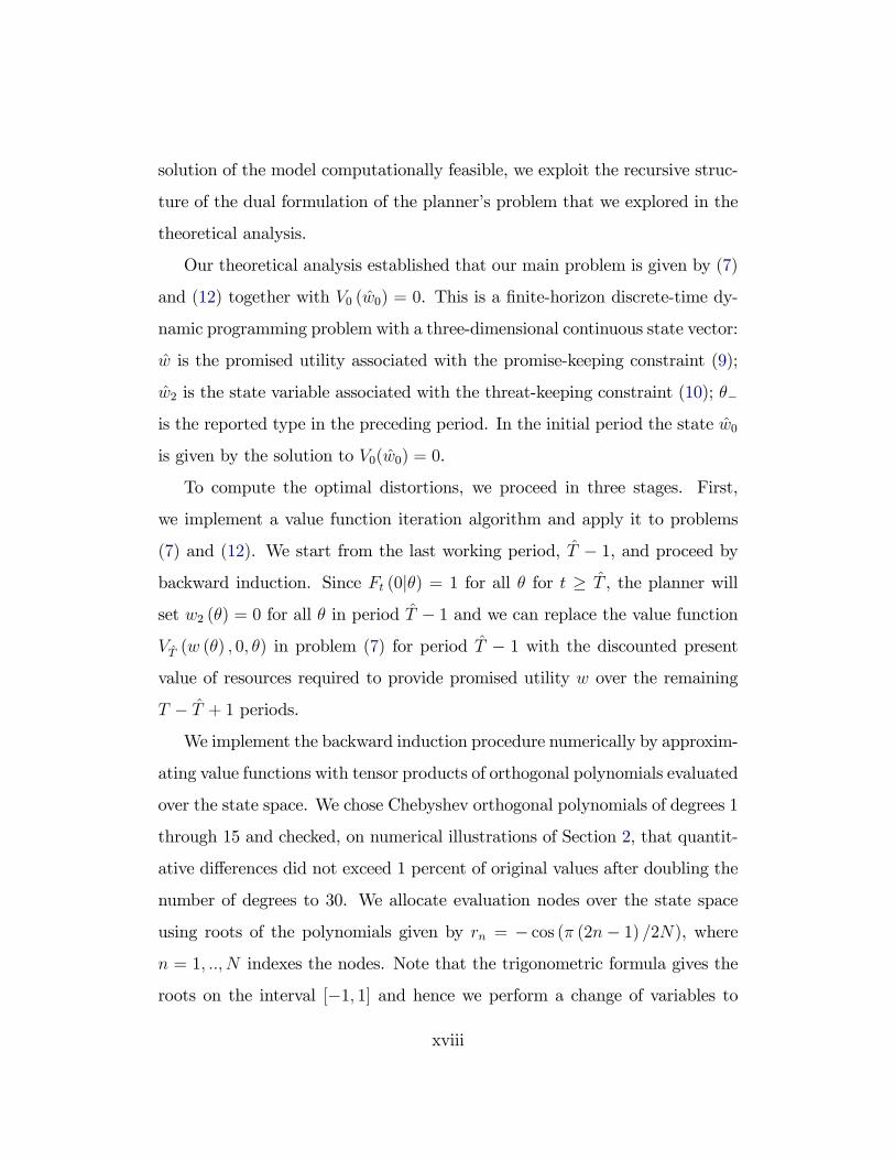
solution of the model computationally feasible, we exploit the recursive struc-

ture of the dual formulation of the planner’s problem that we explored in the

theoretical analysis.

Our theoretical analysis established that our main problem is given by (7)

and (12) together with V0 (w0) = 0. This is a finite-horizon discrete-time dy-

namic programming problem with a three-dimensional continuous state vector:

w is the promised utility associated with the promise-keeping constraint (9);

w2 is the state variable associated with the threat-keeping constraint (10); θ−

is the reported type in the preceding period. In the initial period the state w0

is given by the solution to V0(w0) = 0.

To compute the optimal distortions, we proceed in three stages. First,

we implement a value function iteration algorithm and apply it to problems

(7) and (12). We start from the last working period, T − 1, and proceed by

backward induction. Since Ft (0|θ) = 1 for all θ for t ≥ T , the planner will

set w2 (θ) = 0 for all θ in period T − 1 and we can replace the value function

VT (w (θ) , 0, θ) in problem (7) for period T − 1 with the discounted present

value of resources required to provide promised utility w over the remaining

T − T + 1 periods.

We implement the backward induction procedure numerically by approxim-

ating value functions with tensor products of orthogonal polynomials evaluated

over the state space. We chose Chebyshev orthogonal polynomials of degrees 1

through 15 and checked, on numerical illustrations of Section 2, that quantit-

ative differences did not exceed 1 percent of original values after doubling the

number of degrees to 30. We allocate evaluation nodes over the state space

using roots of the polynomials given by rn = − cos (π (2n− 1) /2N), where

n = 1, .., N indexes the nodes. Note that the trigonometric formula gives the

roots on the interval [−1, 1] and hence we perform a change of variables to

xviii

adjust the root nodes to our state space. We let N = 16 for both the promise,

w, and for the threat, w2. For the skill, we set 30 equally spaced nodes to

capture equally accurately the whole shape of the distribution of distortions

within each period. Chebyshev coeffi cients are then computed by minimizing

the sum of squared distances from the computed values at 7,680 evaluation

nodes.

It is a familiar property of a state space in these problems, that no con-

strained optimal allocations may exist for some nodes. Before proceeding, one

must either implement a state space restriction algorithm to eliminate such

nodes or assign suffi ciently large penalties to such nodes and ensure that large

enough number of nodes are actually computed.18 We implement a heuristic

algorithm combining the features of both methods. First, we choose an arbit-

rarily large state space and attempt to find the optimum at each node. The

nodes where we fail receive minus infinity for the value of the planner (we

use two optimization algorithms on each node with multiple starting points).

Once all nodes are computed we verify that infinite values are along the borders

and replace them with values equal to linearly extrapolated borders, making

these nodes less attractive to the planner than any other computed node, but

preserving the usability of a continuous approximation. If a given period has

more than 77 penalized nodes (1 percent of total for a period) we re-start

by reducing the size of the last period’s state space and continue backwards.

We stopped with the maximum of 0.99 percent and the average of 0.47 per-

cent of penalized nodes per period. To keep the overall computational burden

manageable, we used this procedure rather than a full fixed point search.

The approximation procedure provides each period t problem (7) with a

18For a discussion of both and an implementation of the first method in a related problem

see, e.g., Abraham and Pavoni (2008) and references therein.

xix

continuous function approximating Vt+1, which we write as a tensor product of

the polynomials with their computed coeffi cients. Even though recursive eval-

uation of Chebyshev polynomials is faster (i.e., Pd (r) = 2rPd−1 (r)−Pd−2 (r),

where Pd (r) is the Chebyshev polynomial of degree d > 1 evaluated at r),

we use their trigonometric form in the evaluation of the tensor products (i.e.,

Pd (r) = cos (d arccos (r))). This allows us to apply an implementation of al-

gorithmic (chain rule) differentiation. In contrast, we found that numerical

differentiation methods, e.g., complex step differentiation, resulted in suffi -

ciently large numerical errors to often prevent our optimization algorithms

from converging.

At this stage we also verify the assumptions we made in the theoretical ana-

lysis. Assumption 1 is satisfied analytically given our choices of preferences.

Assumption 2 is satisfied trivially for the parameter values we choose in the

main text. We verify the increasing properties of Assumption 3 numerically

during this computational stage. The assumption requires three increasing

properties of policy functions, c (·), ω (·|θ), and ω1

(θ|·). We compute nu-

merical differences at each node and interpret differences greater than −1e5

as non-negative, satisfying the increasing properties. In addition, we check

that the computed value functions Vt are convex in the promise, w, and in the

threat, w2.

The second stage computes w0 such that V0 (w0) = 0. Given V0 computed

in the first stage, we first search for an interval containing zero using binary

jumps. We start with a high initial promise (e.g., −1e5 for the benchmark

CES case) to ensure that the starting V0 > 0, and scale the initial promise by

2i on the ith iteration until V0 < 0. Then, we converge to w0 with bisection.

We set the numerical error tolerance for the bisection procedure to 1e5 once

again so that a smaller V0 is interpreted to be zero. The rate of convergence

xx

for bisection is linear, however, it is relatively more important at this stage to

guarantee convergence.

In the final stage, we compute optimal labor and savings distortions. Given

Vt’s computed and approximated as continuously differentiable functions in the

first stage and given w0 solved for in the second stage, we generate optimal

allocations by forward induction, starting from policy functions produced by

V0 (w0) from problem (12). Optimal labor and savings distortions are com-

puted from the policy functions using definitions (14) and (15) respectively.

Given a history up to period t, labor distortions can be readily computed by

this procedure with polynomial algorithm complexity. However, computing

savings distortions for a given history up to period t requires computing all

possible t + 1 conditional history realizations. As a consequence, this stage

quickly adds up to exponential algorithm complexity. To keep the problem

computationally feasible and at the same time develop novel insights, we com-

pute several examples of complete histories that we argue are of interest in

Section 3.

Note that for the first and the last stages of this approach to be compu-

tationally feasible, it is essential to use an effi cient and robust optimization

algorithm to solve each of the separate period t minimization problems for

each evaluation node. We solve these problem using an implementation of

the interior-point algorithm.19 We choose conjugate gradient iteration to com-

pute the optimization step. The implementation uses a trust-region method

to solve barrier problems. The acceptance criterion is an l1 barrier penalty

function. Interior-point algorithms are some of the most effi cient and stable

19The implementation we use is KNITRO’s algorithm 1. We implement the model in

AMPL to streamline the application of the algorithm and to take advantage of algorithmic

differentiation.

xxi

methods that are currently available for solving large non-linear optimization

problems. To further improve the accuracy of the solution estimates, includ-

ing Lagrange multipliers, we proceed, at the value function iteration stage, to

active-set iterations that use the output of the interior-point algorithm as its

input. The implementation of the active-set algorithm is based on the sequen-

tial linear quadratic programming. Once the problem is correctly scaled, we

observe quadratic convergence.

Finally, we note that these optimization methods are local. Indeed, we find

that optimizations are sensitive to the initial guess. To reduce the possibility

of picking a non-global local optimum within each minimization problem, we

apply a multi-start globalization heuristic.

xxii