Embed Size (px)
Citation preview
DOCUMENTS DE TRAVAIL - WORKING PAPERS
W.P. 02-12
Redesigning Teams and Incentives: A Real Effort Experiment with Managers of a Merged Company
Claude Montmarquette, Jean-Louis Rullière, Marie-Claire Villeval, Romain Zeiliger
Décembre 2002
GATE Groupe d’Analyse et de Théorie
Économique UMR 5824 du CNRS
brought to you by COREView metadata, citation and similar papers at core.ac.uk
provided by HAL-ENS-LYON
GATE Groupe d’Analyse et de Théorie Économique UMR 5824 du CNRS
93 chemin des Mouilles – 69130 Écully – France B.P. 167 – 69131 Écully Cedex
Tél. +33 (0)4 72 86 60 60 – Fax +33 (0)4 72 86 60 90 Messagerie électronique [email protected]
Serveur Web : www.gate.cnrs.fr
Redesigning Teams and Incentives:
A Real Effort Experiment with Managers of a Merged Company Redéfinir les équipes et les incitations: une expérience avec effort réel avec les cadres
d'une entreprise fusionnée Claude Montmarquettea, Jean-Louis Rullièreb,
Marie-Claire Villevalb, Romain Zeiligerb November 2002
Abstract After a merger, company officials face the challenge to uniform compensation schemes and to redesign teams with managers originating from different incentives and working habits. In this paper, we offer a new way to investigate in post-merger the relationship between executive pay and performance, allowing to dissociate the respective influence of shifts occurring both in compensation incentives and in team composition. The results of a real effort experiment conducted with managers within a large pharmaceutical company show that not only changes in compensation incentives affect performance but also that both managers’ past compensation schemes and company cultures matter for cooperation. The efficiency of a new compensation package is conditional on the reshuffling of teams and the past of incentives within the new teams.
JEL-Code: C81, C92, J33, M52 Keywords: Real effort experiments, Executive compensation, Team-based compensation, Mergers.
Résumé
A la suite d'une fusion, les dirigeants doivent à la fois harmoniser les modes de rémunération et recomposer des équipes avec des cadres habitués à d'autres incitations et modes de travail. Dans cet article, nous présentons une nouvelle manière d'analyser la relation entre rémunération des cadres et performance à la suite d'une fusion d'entreprises, en permettant de dissocier l'influence respective des changements qui portent à la fois sur les incitations salariales et la composition des équipes. Les résultats d'une expérience avec effort réel réalisée avec des cadres d'une grande société pharmaceutique montrent non seulement que les changements d'incitations affectent la performance, mais aussi que la coopération est sensible à la fois aux anciens modes de rémunération et cultures d'entreprise. L'efficience du nouveau mode de rémunération est conditionnée par la recomposition des équipes et le passé des incitations au sein des équipes recomposées.
Mots-clés: expérience à effort réel, rémunération des cadres, rémunération d'équipe, fusions d'entreprises.
a CIRANO and University of Montreal, 2020 rue University, Montreal, (Quebec), Canada, H3A 2A5. Tel: (514)985-4015, Fax: (514)985-4039, [email protected] bGATE, CNRS and University Lumiere Lyon 2, 93 chemin des Mouilles, 69130 Ecully, France. Tel: +33 472 86 60 60, Fax: +33 472 86 60 90, [email protected], [email protected], [email protected] We are greatly indebted to AVENTIS Pharma for having given us the opportunity to organize this experiment and for its managers’ cooperation. We are grateful to Laurent Volpi for his help in conducting this research. Our thanks to David Dickinson for useful comments and suggestions and to Marie-Christine Giroux for editorial assistance.
1. Introduction Within the same industry, there are strong evidences of large heterogeneity across firms’
compensation packages (Hermalin and Wallace, 2001). It is not surprising that after a merger,
difficulties arise due to the firms’ different compensation policies that need to be redesigned.
Furthermore, downsizing and reorganization of production entail a reshuffling of teams and
headquarters, combining executives from the companies involved in the merger. In order to
promote internal social cohesion and a joint performance, mergers usually lead to programs of
statutes harmonization in which executives should be paid according to the same
compensation schemes. But performance also depends on the willingness to cooperate within
teams comprising executives from both of the incoming companies. This willingness to
cooperate may be affected not only by the new incentive schemes but also by team
heterogeneity regarding past compensation practices and working habits or non-market
interactions.
Pitfalls may hamper an empirical analysis of the relationship between new executive pay and
performance in mergers. For example, being aware that history matters (see Nalbantian and
Schotter, 1997), the efficiency of new compensation schemes may differ from an agent to
another depending on the long-lasting influence of his preceding mode of compensation.
Thus, assessing the impact of new compensation schemes on the current executives’
performance in a merger requires to control for a possible long-term impact of the former
compensation packages used in the incoming firms. In addition, unbiased estimations of the
relation between executive pay and performance require disentangling the effect of a shift in
direct incentives and the effect of a change in the characteristics of the group to which the
individuals belong on current performance.
Experimental methods help in circumventing part of these potential difficulties, through a
control of the environment and the comparison of various treatments. This point has been
successfully made in the context of a merger by Weber and Camerer (2001). These authors, in
their laboratory experiment with students, have allowed firms to develop a culture (here
associated with language) before they merge. They showed that performance decreases
following the merger of two laboratory firms.
In this paper, we design an experiment to analyze the relationship between executive
compensation schemes and performance in terms of team cooperation in a merger. The
originality of this experiment is that it is a real-effort experiment conducted with managers of
a merged company. There are few experimental papers studying rewards and team
cooperation in a real work setting. The participants in the laboratory are usually required to
choose an effort level or a contribution level, but they are not requested to produce a real
effort (Bull, Schotter and Weigelt, 1987; Fehr, Gächter and Kirchsteiger, 1997; Güth,
Königstein, Kovacs and Zala-Meso, 2001; Nalbantian and Schotter, 1997, Schotter 1998).
These studies confirm that monetary incentives do matter, but they need to postulate some
equivalence between effort and intention of contribution and between disutility of effort and
money. Dickinson (1999) has used a real effort approach (typing letters) with student-
participants. He has examined labor-leisure decisions in accounting for both the choice of
hours of work and the choice of the effort intensity controlling for changes in hours and
wages. Sillamaa (1999) has shown how student-participants adjust their work (consisting of a
decoding task) in response to changes in wage rates under various tax systems. More related
to our own approach, van Dijk, Sonnemans and van Winden (2001) have conducted an
experiment comparing the incentive effects of individual piece-rate pay, team-based
compensation and rank-order tournaments. Student-participants have to achieve a task
consisting in two-variable optimization for finding the unique peak of a function, which is
solved by a process of trial and error, in a limited period of time. This experiment has allowed
a direct measure of incentives on actual effort level in a controlled environment.
In our experiment, the task required of participants consists in searching the highest value of a
multiple-peaked function in a two-dimensional space. This design makes all participants
simultaneously face the same level of difficulty. The novelty of the task ensures that nobody
benefits from a previous learning advantage. Moreover, each participant cannot use a single
heuristics for reaching each peak at minimum cost. The task to perform has a cognitive
component since, along with the intensity of the concentration required, there is a monetary
cost linked to the chosen speed of progression.
This laboratory experiment has been conducted with 36 managers in the headquarters of a
large pharmaceutical company resulting from the recent merger of a French and a German
company. With the implication of executives and not students, we escape the
representativeness issue. This is often pointed out by those unfamiliar with experimental
economics who are particularly concerned with the difficulty of translating the results of
experiments with student-participants into a firm’s policy. However, this approach also differs
from natural experiments (for example, Lazear, 2000) or field experiments (Erev, Bornstein
and Galili, 1993; Shearer, 2001): in our experiment, the managers take their decisions in an
artificial environment (anonymous interactions, no context, neutral wording).
The experimental design consists in two parts of ten periods each, played under a stranger
protocol. In the first part, teams are homogeneous, i.e. members belong to the same incoming
firm with the compensation scheme used before the merger. In the second part of the
experiment, we have two alternative treatments to introduce the compensation scheme after
the merger. In one treatment, the teams remain homogenous as in the first part of the
experiment. In the other treatment, the teams are formed with participants originating from the
two merged companies. For each period, a team consists in three participants who have to
perform the same task under the same incentive scheme.
The econometric analysis of the experimental data controls for tiredness, learning, differences
in ability and chance. Experimental evidence shows that changes in compensation incentives
affect performance and that both managers’ past compensation schemes and company cultures
(Kreps, 1990) matter for cooperation. Furthermore, the concept of job challenge emerged as
an interesting issue in soliciting more effort from the participants.
In Section 2, the design of the real effort experiment is outlined. In Section 3, we present the
experimental procedures. The econometric estimations and the empirical results are presented
in Section 4. In Section 5, we summarize and conclude.
2. Experimental design
We will successively present the design of the task to be performed by the participants, the
structure of the payment schemes, the various experimental treatments and the information
conditions.
2.1. Design of the task
In our experiment, effort must be captured by means of a task able to mimic some aspects of
the content of a manager’s job (namely concentration, adjustment of means to targets,
variability). This task must solicit an effort and avoid boredom to keep the managers in our
company interested. At the same time, it cannot be too complex to limit the differences in
abilities between the participants. The challenge is to be able to discriminate the impact of
effort on the outcome from that of ability. In addition, the outcome itself has to be easily and
directly measurable by the participants and not only by the experimenter. The task consists in
searching for the highest value of a multiple-peaked function in a two-dimensional space
defined vertically by altitude (A) and horizontally by distance (D) from the origin, with
[ ]0,100A ∈ , [ ]0,300D ∈ and with ( )MaxA f D= . The successive cubic Bezier curves that
correspond to this function are weakly increasing, with three local peaks.1 The flexibility of
this form permits a variety of curves.
During a fixed time period, the subject progressively uncovers the curve on his computer
screen by clicking a button repeatedly or by holding the mouse button down2. Search starts at
the origin (0,0). The subject moves by discrete steps of 1 on the horizontal axis that make him
go ahead; coming back is impossible. Thus, search does not proceed by trial and error. The
subject can stop his progression whenever he wants. When the period starts, the rectangular
box in which the curve will progressively appear is fully black. The curve and its surface
become visible as the subject progresses on the horizontal axis.
Thus, the individual effort is captured through the willingness to reach local peaks whose
abscissas at the origin are unknown to the participant. But effort is also captured through a
cost parameter. The idea is that effort is costly and more effort entails more costs. Cost is
represented in our experiment through the choice of the speed of progression, i.e. the work
pace. Parameters are chosen so that it is impossible to reach the maximum altitude during the
one-minute period allowed by using the regular speed only; the regular speed allows covering
a maximum distance of 195. Whereas each 1-step (the regular speed) is free, each 2-step (the
rapid speed) entails a cost of 0.4 point. The subject can switch speeds whenever he wants and
without any restriction in frequency.
1 This curve is defined as a succession of several cubic Bezier curves, each defined by four points, two endpoints with ( )0 0,x y as the origin and ( )3 3,x y as the destination endpoints, and two control points
( )1 1,x y and ( )2 2,x y . Two equations define the points on each curve, one yielding values for x, the other for y:
( )( )
3 20
3 20
x x x
y y y
x t a t b t c t x
y t a t b t c t y
= + + +
= + + +
At the origin, the slope of the curve is tangent to the line between ( )0 0,x y and ( )1 1,x y and at destination, its
slope is tangent to the line between ( )2 2,x y and ( )3 3,x y . 2 In their experiment, Van Dijk et al. introduce a lag of 1.5 seconds between two moves in order to reduce the advantage of experienced players on computer games. Here, moves can proceed continuously so that the experienced computer players do not have a specific advantage.
[Insert figure 1 about here] Fig. 1 depicts the screen available to the participants. As soon as a new period starts, the
screen indicates currently the time left and the cumulated cost of 2-steps. Two buttons are
available, one for each of the two possible speeds. Different thresholds in altitude are
indicated on the curve. The curve appears in the black box and the surface of the curve takes
different colors progressively according to the altitude reached, each color corresponding to a
level of payoff, as explained next. Intensity of color below the curve is greater when 1-steps
are used.
2.2. Effort and payment schemes
The game involves teams consisting in three participants, which have to uncover the same
curve. Within a team, each subject has to perform the task on his own but his payoff depends
on both individual and collective performances. Individual payoff is given by the sum of three
elements whose amount and relative proportion depend on the stage of the game and on the
treatment. In a given stage and treatment, i F I Tα α α απ = + + , with { },X Yα = , X and Y
corresponding to incoming firms.
• Fα is a fixed-wage earned by subject i as soon as his individual outcome reaches a first
threshold, min1A , defined by the altitude reached.
• Iα is an individual target award earned if i’s outcome reaches a second threshold, min2A
with min min2 1A A> .
• Tα is a team reward obtained when the sum of individual outcomes within the team
reaches a third threshold, min3A , with min min min
3 2 13 3A A A> > . In contrast with the two
former elements, a subject may earn this reward even though she does not contribute
an effort greater than the effort giving her the fixed wage or the individual target
award. It raises a free-riding incentive. However, the value of the third threshold is
chosen so that the team reward cannot be obtained if the subject produces an outcome
lower than the first threshold.
The combination of these three elements defines a compensation package that reproduces the
total compensation plan in use in the pharmaceutical company3. As soon as one element of the
compensation package is reached, the surface of the curve in the screen box takes a new color.
If there is no piece-rate wage in this design, individual target awards and team-based rewards
can be considered as variable compensation since they are linked to performance targets
beyond a standard requirement. In contrast, Fα represents a fixed-payment for the
performance requirement and is usually rather low. It can always be achieved with costless
steps in the time allowed. An employer would consider a lack of effort, below this level of
performance, a professional misconduct.
One aspect of managers’ work is the ability to deal with uncertainty. Thus, we have used
different curves, more or less difficult, at each repetition of the game. During each period of a
session, all participants worked with the same curve and this was common knowledge within
the teams. It allows us to compare the performance achieved by the different participants and
groups. Because of the structure of the compensation package, the difficulty of a curve
depends on its shape and on the abscissa at the origin of the various thresholds triggering
rewards4.
3 The plan has four parts. A base salary reflecting performance, skill, competency level and seniority. An Annual Incentive Plan (short-term incentives), which provides rewards to eligible associates for reaching predetermined targets. Long-term incentives consist in stock options dedicated to eligible grade level employees. Other employee benefits provide additional protection in case of sickness or after retirement. However, this total compensation plan, as extensive as it can be, may clash with former compensation traditions of the incoming firms. Pre-merger compensation schemes differed largely between firms. In one firm, executives were compensated by a fixed wage and target rewards, but in a proportion different than in the merger. In contrast, executives from the other firm were only compensated by a fixed wage at a level competitive with comparable pharmaceutical companies. 4 The index of difficulty of each curve, denoted jd is given by: ( ) ( ) ( )2 2
1 2 1 3 2jd D D D D D= + − + − with 1D the abscissa at the origin of the first threshold, 2D the abscissa at the origin of the second threshold and
3D the abscissa at the origin of the maximum altitude. The more distant from the origin the first threshold and the greater distance between the first and the second thresholds, the more difficult it is to reach additional rewards.
Therefore, to allocate her effort, a participant has to consider five elements: her expectation
about the shape of the curve that she progressively uncovers, the cost she is willing to bear to
speed up his progression, the moment where it is more profitable to use costly steps
depending on the steepness of the slope, and her expectation about the willingness of her
team-mates to reach the collective reward5.
2.3. Experimental treatments
Let us consider the timing of the game and the various treatments.
A session has two parts of 10 periods each, with a random order of presentation of the various
curves. In the first part, each team faces the payment scheme used in their company before the
merger. As shown in Table 1, for the X teams, the proportion of the fixed wage in total
possible rewards is lower than for the Y teams who cannot receive any individual target
awards. Thus, individual incentives are lower for the Y teams. In contrast, for all teams, the
same performance is required for triggering the fixed payment and the team reward. A
maximum of 100 ECU (Experimental Currency Unit) can be earned.
In the last ten periods, the compensation scheme for all participants is the one used after the
merger. To avoid a loss aversion hindering motivation, the change introduced preserves the
absolute level of each previous component of the compensation package, by increasing the
maximum payoff achievable from 100 to 120 ECU6. Compared to the rules applied among the
X teams in the first ten periods, besides the thresholds, the compensation package also
includes a fixed payment, an individual target award and a team reward. In contrast, the fixed
payment is increased in order to equalize the one formerly used for the Y teams. Compared to
the rules of the Y participants in the first ten periods, the fixed payment remains constant but
5 Uncertainty is not subject-specific and this can be accounted for in the empirical estimations through the index of difficulty of the curve. In contrast, the rationality involved in the choice of the fast speed option indicates that there may be some differences in ability among participants. Empirical estimations must also control for a likely learning effect. 6 This increase is not unrealistic since acquisition activities are more likely to be followed by employment losses than by wage cuts (see, for example, Conyon et al., 2002).
an individual target award is added. Thus, the individual incentive of the Y participants is now
increased, whereas it is lowered for the X participants.
Two treatments have been run, the mixed-treatment and the fixed-treatment. The first part is
similar in both. These treatments only differ in the composition of teams in the second part of
the session. In the mixed-treatment, teams may gather executives from both incoming
companies. In the fixed-treatment, teams remain homogeneous, i.e. teams gather executives
only from the same incoming company. Thus the fixed-treatment serves as a baseline against
which the effect of the merger beyond the shift in private incentives can be tested. In any case,
a stranger protocol is used, whatever the treatment and the period: each new period entails a
reshuffling of teams, either within the same category (part 1 and part 2 in the fixed-treatment)
or between categories (part 2 in the mixed-treatment).
[Insert Table 1 about here]
2.4. Information conditions
Under the mixed-treatment, all participants were informed of the existence of two categories
of participants in equal numbers in the room, “X” and “Y”, but they were unaware of the
meaning of these labels. They learned their own identity by reading the instruction sheet and
they were informed that they would keep the same identity throughout the session. The
instruction sheet for the first 10 periods also mentioned that they were matched with two other
participants belonging to the same category as themselves but that the composition of this
group was changed each new period within the same category. The participants knew the
description of the task to be performed and the payoff structure applicable to their category.
They were aware that the same task was to be achieved by the three members of the group but
they had no current information on the simultaneous progression of their teammates on the
curve. They got no information about the task or the payoff structure of the other category of
participants. They knew that they would never get any information about the identity or the
payoff of their successive teammates. At the end of each period, a historic table gave each
subject a feedback on his own outcome, the outcome (the cumulated altitude) performed by
his group, his total cost, whether he obtained the various pieces of the compensation package,
and his total payoff net of costs.
In the second part of the session, participants were informed about the payoff structure that
was in use during the first part for each of the two categories: participants X (Y) learned how
participants Y (X) were paid during the first ten periods for the same task to be achieved. This
procedure recreates the psychological concept of “in-group/out-group” which might affect the
cooperative behavior of participants (see Tajfel, Flament, Billig and Bundy, 1971)7.
Moreover, participants were informed of two changes: a group may gather both X and Y
participants for the remaining periods and a new payoff structure is common to all
participants.
When the game was played under the fixed-treatment, participants were unaware of the
coexistence of two categories of participants paid under different rules in the room. They were
only informed that they were being matched to two other same-type participants in a group
and that the group was reshuffled for each new period.
4. Experimental procedures
The experiment was funded by the Human Resources department of the new company and we
benefited from its support in recruiting executives. A sample of 36 volunteer executives was
created, consisting of 18 managers from each incoming firm, representing a large diversity of
departments to limit uncontrolled peer group effects (see Table 2).
7 It was also important not to disturb the effort choices of the first part of the session by comparisons with the other category’s payment schemes, since we wanted to isolate the effect of initial compensation packages in each firm.
[Insert Table 2 about here] The experiment was conducted in November 2001 in Paris, France, in the headquarters of the
merger. Three sessions were organized the same day to limit dissemination of information. In
the first two sessions, the mixed-treatment involved 24 participants in total and in the third
session, 12 participants played in the fixed-treatment. On average, a session lasted 75 minutes
including initial instructions and practice periods. The experiment was computerized using the
REGATE program.8
Running the experiment with managers instead of students requires higher payoffs because of
greater opportunity costs. Transactions were conducted in Experimental Currency Units, with
ECU convertible to Euros at the rate 100 ECU = 3 €. A show-up fee of 8 € was added. On
average, a subject earned 51.45 € (S.D.=3.75), so that total payoffs amounted to 1844 €.
Participants were paid a few days later with vouchers, exchanged against the ticket given to
them by the experimenter at the end of each session to preserve confidentiality.
Upon arrival, each participant had to register and was invited to draw a ticket that assigned
her a computer from an envelope. There were in fact two envelopes presented to participants
according to their origin, A or B, but participants were unaware of this allocation rule. At the
same time, the participants discovered a set of written instructions for the first part of the
session under their keyboard. As the payment schemes differed among X and Y participants,
the experimenter did not read the instructions aloud (see Appendix A). The instructions were
phrased in neutral terms (we spoke about a curve, a group, a payoff, an outcome, and we
avoided loaded terms such as effort, contribution and wage). Participants were allowed to ask
questions, which were answered in private. Then, three practice periods were run before the
8 Developed at GATE (Groupe d’Analyse et de Théorie Economique, CNRS and University Lumière Lyon 2, France).
first part began. At the end of the first part, the game stopped and further instructions for the
second part were distributed, without any questions allowed.
5. Experimental results
In the pre and post merger situations reproduced in the laboratory, the results of this
experiment identify the determinants of the effort levels deployed by the participants. They
explain why some participants choose the costly 2-step procedure more often than others.
These results also show the impact of redesigning the compensation structure and the team
composition on these levels. It enables us to assess the efficiency of a new compensation
package conditional on the reshuffling of teams and on past incentives within the new teams.
Economic theory predicts that monetary incentives enhance effort. However, with team
compensation, the theory also predicts a robust free riding behavior of participants within the
team both in the effort levels and in the cost incurred. Thus, participants should stop moving
or incurring costs as soon as they reach the first threshold if they belong to a Y team in the
first part, or the second threshold in all the other cases. With the difficulties created by
conflicting cultures in mergers (Weber and Camerer, 2002), we should expect lesser efforts
and lower costs and a reduced cooperation attitude after the merger.
5.1. Data and descriptive statistics
Table 3 presents the definition and descriptive statistics of the variables used in the empirical
analysis of the experimental data.
[Insert Table3 about here]
The endogenous variables “effort levels” and “costs” are directly observable. Cost adds a
cognitive component to the task requiring more concentration than keeping a finger on a
costless key to advance on the curve, since it requires the participants to allocate their costly
steps as a function of the difficulty of the curve. It also introduces an additional strategic
dimension for team cooperation.
“Intensity of preference for cooperation” is a latent variable. The observable counterpart
values for this variable at each period and for each participant are set at 0 for an
uncooperative participant, 1 for a cooperative participant, and 2 for a very cooperative
participant. These credentials are obtained under the following conditions. For part 1 (i.e. the
set of periods 1 to 10), X is qualified as uncooperative in period t when her level of effort, XE ,
is 60≤ , i.e. when she does not contribute to the team outcome beyond the level that triggers
her individual reward. The same condition applies for part 2 (i.e. the set of periods 11 to 20).
For part 1, Y is qualified as uncooperative when her effort in period t is 40≤ , and for part 2
when her effort in period t is 60≤ . X is said to be cooperative when her effort in period t is
60 80xE< ≤ in part 1, 80 being the average individual effort required to trigger the team
reward. The same condition applies for part 2. Y is said to be cooperative when her effort in
period t is 40 80yE< ≤ in part 1. For part 2, her required level of effort in period t is
60 80yE< ≤ . Finally, X and Y are very cooperative in period t when their respective effort is
80> , i.e. when they continue contributing beyond the average effort triggering the team
reward.
The exogenous variables are the period, the type of participants, the mode of compensation,
the composition of groups (either fixed or mixed) and an index of difficulty for each curve.
The lagged effort level of the other members of the group is a reciprocity variable to assess
whether members modulate their efforts to what the other members of the group did in the
previous period. Since the experiment is run with randomly re-matched partners at each
period, this reciprocity may develop within the whole category of participants.
Interaction variables involving the Y participants are created to test whether X and
participants Y behave differently during the different parts of the experiment. They reflect
many situations captured in the forthcoming regressions. The coefficient estimates of the
variable “mode of compensation in part 1” report the decisions of the X participants in part 1
relatively to their decisions in the mode of compensation in part 2 (element of the constant
term). With the coefficients of the “mixed session” variable, we further distinguish the
decisions of X participants in the mixed sessions of part 2 relatively to the fixed sessions of
part 2. The decisions of Y participants in part 1 are the sum of the coefficients of the variables
“participant Y”, “mode of compensation in part 1” and “participant Y and mode of
compensation in part 1”. This last variable is needed as the modes of compensation differ in
part 1 between X and Y participants. Summing-up the coefficient estimates of the variables
“participant Y”, “mixed session” and “participant Y and mixed session” gives the decisions of
Y participants in the mixed sessions in part 2. The coefficient of the “participant Y” variable
shows the decisions of Y in the fixed sessions in part 2.
The index of difficulty and the period variables enter the regressions with interacting variables
and nonlinear forms. The variable “logarithm of the period”, for example, accounts for
potential fatigue and on-the-job leisure .
5.2 Econometric results
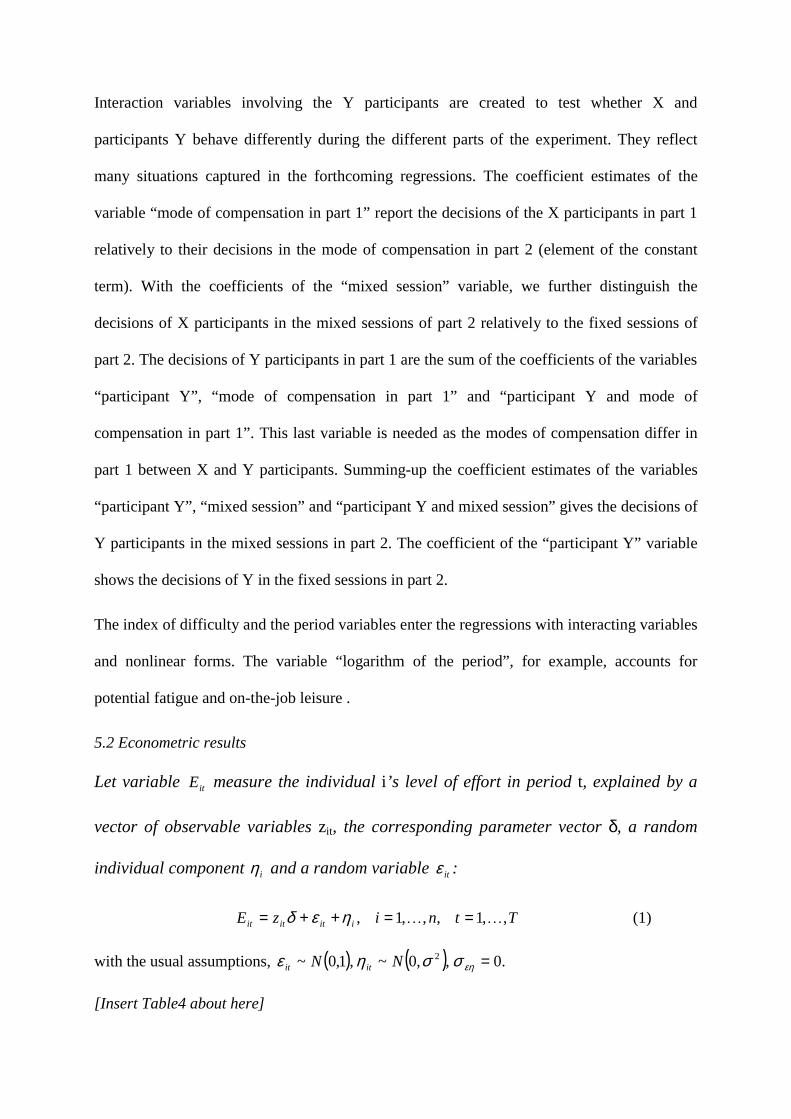
Let variable itE measure the individual i’s level of effort in period t, explained by a
vector of observable variables zit, the corresponding parameter vector δ, a random
individual component iη and a random variable itε :
TtnizE iititit ,,1,,,1, �� ==++= ηεδ (1)
with the usual assumptions, ( ) ( ) .0,,0~,1,0~ 2 =εησσηε NN itit
[Insert Table4 about here]
Column 1 of Table 4 displays the results of a linear one-way random effects model on the
participants’ effort levels. We observe a significant and substantial increase in the effort levels
by both participants X and Y in part 2 relatively to the first part. A higher pay rate and
changes in the structure of compensation have increased the level efforts by almost 12 points.
Reciprocity, an outcome generally observed in teams (Fehr and Falk, 2002), is also present in these results. However, reciprocity concerns only the Y participants. An increase in the effort levels by the other members of the group in the preceding period motivates the Y participants to reciprocate by increasing their own level of effort. Although not highly statistically significant (at the 15% level only), it is nevertheless interesting to note the negative coefficient of the interaction variable “participant Y and Mixed”: Y participants, knowing that they may be interacting with X participants, have a tendency to lower their effort levels. The index of the difficulty of the curves does not affect the effort levels in a linear way. The
observed U-shape curve suggests that across all compensation schemes, more difficult tasks
may actually elicit, to some extent, more effort by all types of managers. This job challenge
effect is present even in the late stage of the experiment (see the “index of difficulty and
period” crossed variable). The effort levels decrease with the number of periods played (also
in a nonlinear way) suggesting that fatigue and on-the-job leisure eventually play a role.
These relationships suggest that the production and the allocation of effort as a function of the
degree of difficulty change over time: while fatigue exerts a negative effect on the production
of effort, the agent is more and more reactive to the job challenge over time. Finally, a
negative first period effect on the effort levels may reflect a preliminary cautious attitude.
However, the analysis of the sole effort levels is not sufficient to inform us about the
willingness of the agents to cooperate. In order to appreciate this aspect, it can be necessary to
refer the actual levels of effort to the ranking of compensation thresholds, by studying the
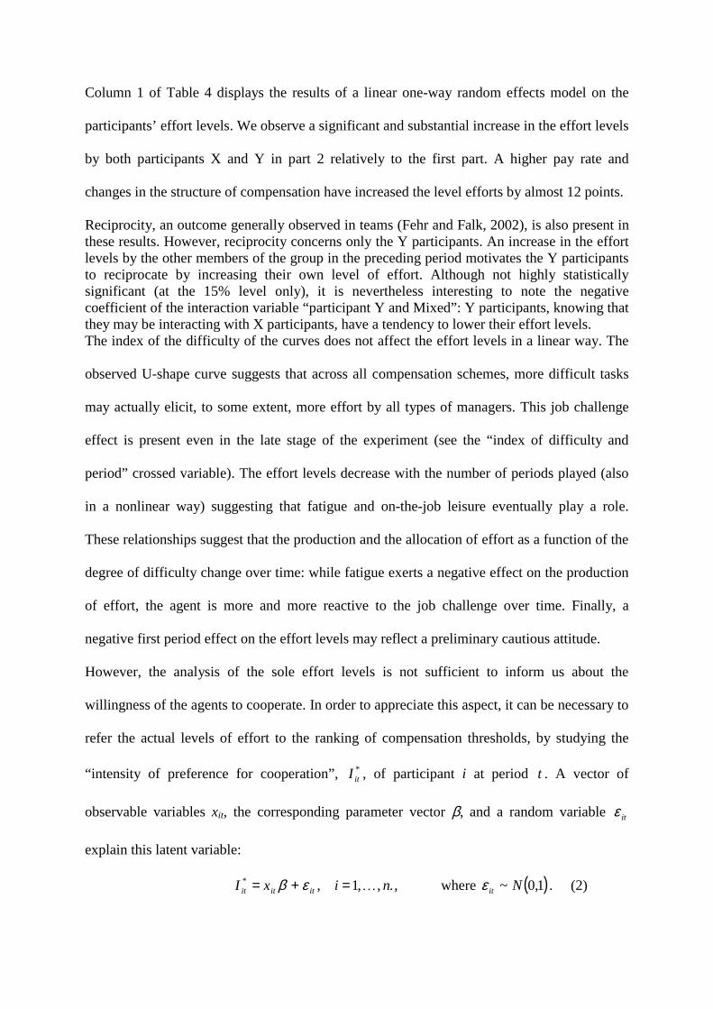
“intensity of preference for cooperation”, *itI , of participant i at period t . A vector of
observable variables xit, the corresponding parameter vector β, and a random variable itε
explain this latent variable:
.,,1,* nixI ititit l=+= εβ , where ( )1,0~ Nitε . (2)
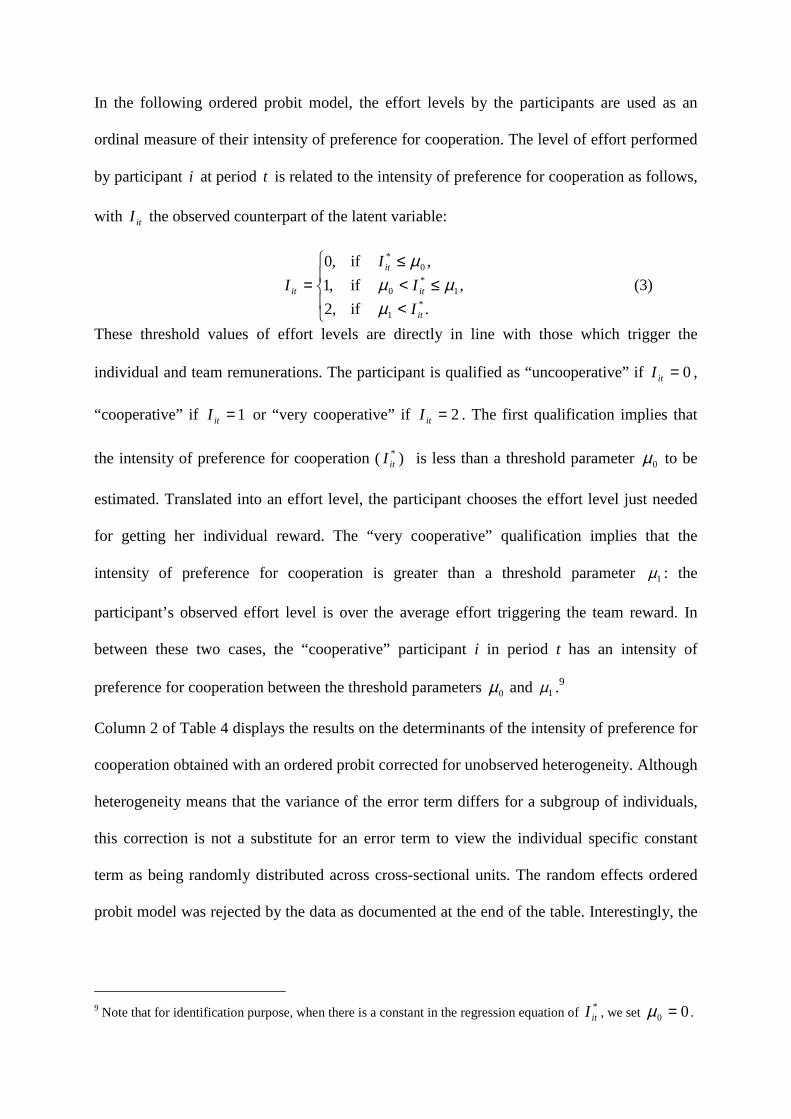
In the following ordered probit model, the effort levels by the participants are used as an
ordinal measure of their intensity of preference for cooperation. The level of effort performed
by participant i at period t is related to the intensity of preference for cooperation as follows,
with itI the observed counterpart of the latent variable:
<≤<
≤=
.if,2,if,1
,if,0
*1
1*
0
0*
it
it
it
it
II
II
µµµ
µ (3)
These threshold values of effort levels are directly in line with those which trigger the
individual and team remunerations. The participant is qualified as “uncooperative” if 0=itI ,
“cooperative” if 1=itI or “very cooperative” if 2=itI . The first qualification implies that
the intensity of preference for cooperation ( *itI ) is less than a threshold parameter 0µ to be
estimated. Translated into an effort level, the participant chooses the effort level just needed
for getting her individual reward. The “very cooperative” qualification implies that the
intensity of preference for cooperation is greater than a threshold parameter 1µ : the
participant’s observed effort level is over the average effort triggering the team reward. In
between these two cases, the “cooperative” participant i in period t has an intensity of
preference for cooperation between the threshold parameters 0µ and 1µ .9
Column 2 of Table 4 displays the results on the determinants of the intensity of preference for
cooperation obtained with an ordered probit corrected for unobserved heterogeneity. Although
heterogeneity means that the variance of the error term differs for a subgroup of individuals,
this correction is not a substitute for an error term to view the individual specific constant
term as being randomly distributed across cross-sectional units. The random effects ordered
probit model was rejected by the data as documented at the end of the table. Interestingly, the
9 Note that for identification purpose, when there is a constant in the regression equation of *
itI , we set 00 =µ .
coefficient of the Y dummy variable used to correct for heterogeneity10, is negative and
statistically significant. Thus the variance of the error term in the intensity of preference for
cooperation is lower for the Y participants than for the X participants. They form in that sense
a more homogenous group than the X participants.
In part 2, the level of cooperation improves over the initial structures of compensation as
shown by the negative and highly statistically significant coefficient estimate of the “mode of
compensation in part 1” variable. This also holds for the Y participants who have seen an
individual target award added for them in this part. These results are coherent with the higher
effort levels deployed with the mode of compensation in part 2.
Reciprocity plays a role for both types of participants: an increase in the level of efforts of
others in the previous period creates an additional motivation for both the X and Y
participants to cooperate. This was observed for the Y participants with regards to the effort
levels. In mixed sessions, the Y participants tend to reduce their intensity of cooperation with
the coefficient of the corresponding variable statistically significant at 11.1%. In other words,
these results temper the differences in terms of effort regarding Y participants’ strategy. The
differences may be accounted for by the fact that, in the model, the intensity of preference for
cooperation is defined by means of broad intervals. Once a threshold is reached, the level of
cooperation is changed but the effort levels may differ among participants. Like in the effort
level regressions, the relationship between the difficulty of the curve and the intensity of
preference for cooperation follows a U-shape. There is no first period effect, and not
surprisingly cooperation declines with the later periods.
Finally, column 3 of Table 4 reports the results on the determinants of the cost levels decided
by the participants. The econometric estimates are also obtained with a linear one-way
10 A gender variable was also tried, but it was statistically insignificant.
random effects model as defined by equation (1), after substituting itC for the dependent
variable. Incurring a cost means using a 2-step procedure to achieve the task. One attention-
grabbing result implies the Y participants. Ceteris paribus, while in part 2 the X participants
increase their costs in a mixed session by 6.22 units relatively to a fixed session, the Y
participants substantially reduce their costs by 8.37 units11 when they may interact with X
participants. As noted in the previous discussion on the effort levels, it seems that the Y
participants change their strategy when being informed that they may be teamed up with X
participants. In contrast, the X participants are not influenced by this dimension. It isolates the
direct effect of team redesigning, independently of the shift in compensation incentives.
The relationship between the difficulty of the curves and the costs supported by the
participants indicates an reverse U-shape. If the task is too difficult, the participants increase
their efforts as we saw earlier, but they do so without resorting to the 2-step costly moves.
This result reinforces our preceding analysis of the level of effort: an increased difficulty does
not discourage effort under the condition that the participants can save on their costs. Lastly,
there is a positive first period effect on the cost levels, but costs decline more linearly as the
experiment evolves, possibly due to a learning effect.
The cognitive approach of this real effort experiment has anchored the analysis of cooperation
within a team through three dimensions identifying the notion of effort: level, thresholds and
cost. The econometric estimates based on these three elements do not reveal contradictions or
paradoxical effects: most agents determine their level of effort as a function of the structure of
compensation, the difficulty of the task and their tiredness. But the experiment reveals that a
category of participants (i.e. the Y participants) also modulate their efforts with respect to the
composition of their team in terms of origin. 11 This result derives from the following calculus: [8.04 – (8.04 + 6.22 – 14.59)]. The first term corresponds to the coefficient of the variable for participants Y in part 2 when groups are fixed. The second term represents the value of the coefficients for participants Y in part 2 when groups are mixed.
6. Conclusion
Executive behavior with respect to performance and cooperation is a major element in the
success or failure of a merger between two companies. Economists traditionally have
suggested to look for an adapted compensation policy to facilitate cooperation and renewed
efforts from groups of individuals coming from different corporate cultures. The aim of this
paper is to check whether a harmonization of compensation packages is sufficient to motivate
all managers to cooperate to the same extent. A laboratory experiment has been run involving
managers of two large companies that recently went through a merger. The experimental
design has introduced various compensation schemes that were implemented in the context of
a real effort. Like in most mergers, these managers-subjects have experienced the redesigning
of both compensation schemes and team composition in their newly merged company. The
experimental protocol reproduced the situation before and after the merger in neutral terms
(without any loaded terms).
The results show that financial incentives do work in improving effort and cooperation among
participants, in accordance with standard results (Prendergast, 1999). However, these
incentives are not entirely sufficient to create cooperation among heterogeneous groups. The
past matters, as we have seen that individuals having shared different experiences and coming
from different cultures tend to react differently in the mixed treatment part of our experiment.
This may also result from various manager selection policies in the originating companies.
This suggests that shifting team composition (i.e. mixing managers with different cooperate
cultures) may limit, at least in the short run, the efficiency of a new unified compensation
policy, if not taken into account. Merging cultures requires more time than merging
incentives.
This real effort experiment also shows that introducing a complex task is not necessarily
detrimental to more effort and cooperation. The concept of job challenge is perhaps more

important to solicit greater effort and cooperation among employees than what is anticipated
in the current literature on this subject.
Using managers also has its drawback. The study would have greatly benefited from more
treatments and more observations. A companion study using students from different groups
and countries will look for a confirmation of our results and explore more issues associated
with the idea of cooperation among heterogeneous groups, the different compensation
schemes and the concept of job challenge.
References
Bull, C., Schotter, A., Weigelt, K., 1987.Tournaments and Piece-Rates: An experimental Study. Journal of Political Economy 95, 1-33.
Conyon, M.J., Girma, S., Thompson, S., Wright, P.W., 2002. The Impact of mergers and acqisitions on company employment in the United Kingdom. European Economic Review 46, 31-49.
Dickinson, D.L., 1999. An Experimental Examination of Labor Supply and Work Intensities. Journal of Labor Economics 17 (4), 608-638.
Erev, I., Bornstein, G., Galili, R., 1993. Constructive Intergroup Competition as Solution to the Free Rider Problem: A Field Experiment. Journal of Experimental Social Psychology 29, 463-478.
Fehr, E., Gächter, S., Kirchsteiger, G., 1997. Reciprocity as a Contract Enforcement Device: Experimental Evidence. Econometrica 65, 833-860.
Fehr, E., Falk, A., 2002. Psychological Foundations of Incentives. European Economic Review 46, 687-724.
Güth, W., Königstein, M., Kovacs, J., Zala-Mezo, E., 2001. Fairness Within Firms: The Case of One Principal and Multiple Agents. Schmalenbach’s Business Review 53, 82-101.
Hermalin, B.E., Wallace, N.E., 2001. Firm performance and Executive Compensation in the Savings and Loan Industry. Journal of Financial Economics 61, 139-170.
Kreps, D., 1990. Corporate Culture and Economic Theory. In J. Alt and K. Schepsle (Eds.), Perspective on Positive Political Economy, Cambridge, Cambridge University Press, 90-143.
Lazear, E.P., 2000. Performance Pay and Productivity. American Economic Review 90 (5), 1346-1361.
Nalbantian, H.R., Schotter, A., 1997. Productivity under Group Incentives: An Experimental Study. American Economic Review 87, 314-341.
Prendergast, C., 1999. The Provision of Incentives in Firms. Journal of Economic Literature XXXVII (1), 7-63.
Schotter, A., 1998. Worker trust, system vulnerability, and the performance of work groups. In A. Ben-Ner and L. Putterman (Eds.), Economics, Values and Organization. Cambridge, Cambridge University Press, 364-407.
Shearer, B., 2001. Piece-Rates, Fixed Wages and Incentives: Evidence from a Field Experiment. Université Laval, Québec, Working Paper.
Sillamaa, M.A., 1999. How Work Effort Responds to Wage Taxation: An Experimental Test of a Zero Top Marginal Tax Rate. Journal of Public Economics 73, 125-134.
Tajfel, H., Flament, C., Billig, M.G., Bundy, R.P., 1971. Social Categorization and Intergroup Behavior. European Journal of Social Psychology 1, 147-175.
Van Dijk, F., Sonnemans, J., van Winden, F., 2001. Incentives Systems in a Real Effort Experiment. European Economic Review 45, 187-214.
Weber, R.A., Camerer, C.F., 2002. Cultural Conflict and Merger Failure: An Experimental Approach, Carnegie-Mellon University and California Institute of Technology, unpublished paper.
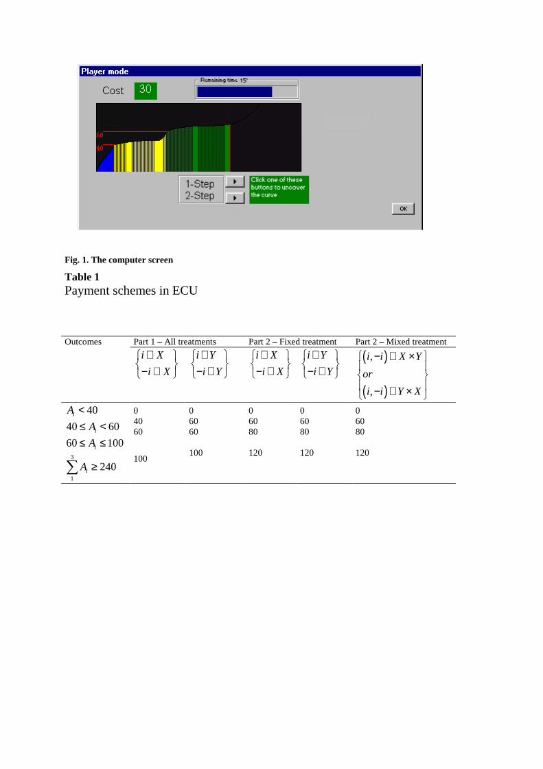
Fig. 1. The computer screen
Table 1 Payment schemes in ECU
Outcomes Part 1 – All treatments Part 2 – Fixed treatment Part 2 – Mixed treatment i X
i X∈
− ∈
i Yi Y∈
− ∈
i Xi X∈
− ∈
i Yi Y∈
− ∈ ( )
( )
,
,
i i X Yori i Y X
− ∈ × − ∈ ×
40iA <
40 60iA≤ <
60 100iA≤ ≤ 3
1240iA ≥∑
0 40 60
100
0 60 60 100
0 60 80 120
0 60 80 120
0 60 80 120
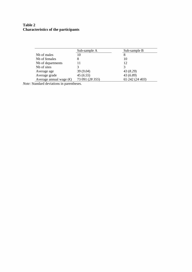
Table 2 Characteristics of the participants
Sub-sample A Sub-sample B Nb of males Nb of females Nb of departments Nb of sites Average age Average grade Average annual wage (€)
10 8 11 3 39 (9.04) 45 (6.55) 73 091 (28 355)
8 10 12 3 43 (8.29) 43 (6.89) 65 242 (24 403)
Note: Standard deviations in parentheses.
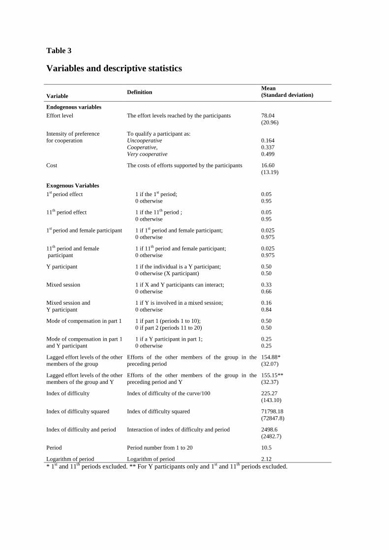
Table 3
Variables and descriptive statistics
Variable Definition
Mean (Standard deviation)
Endogenous variables Effort level The effort levels reached by the participants 78.04
(20.96)
Intensity of preference for cooperation
To qualify a participant as: Uncooperative Cooperative, Very cooperative
0.164 0.337 0.499
Cost
The costs of efforts supported by the participants 16.60 (13.19)
Exogenous Variables 1st period effect
1 if the 1st period; 0 otherwise
0.05 0.95
11th period effect
1 if the 11th period ; 0 otherwise
0.05 0.95
1st period and female participant 1 if 1st period and female participant; 0 otherwise
0.025 0.975
11th period and female participant
1 if 11th period and female participant; 0 otherwise
0.025 0.975
Y participant 1 if the individual is a Y participant; 0 otherwise (X participant)
0.50 0.50
Mixed session
1 if X and Y participants can interact; 0 otherwise
0.33 0.66
Mixed session and Y participant
1 if Y is involved in a mixed session; 0 otherwise
0.16 0.84
Mode of compensation in part 1 1 if part 1 (periods 1 to 10); 0 if part 2 (periods 11 to 20)
0.50 0.50
Mode of compensation in part 1 and Y participant
1 if a Y participant in part 1; 0 otherwise
0.25 0.25
Lagged effort levels of the other members of the group
Efforts of the other members of the group in the preceding period
154.88* (32.07)
Lagged effort levels of the other members of the group and Y
Efforts of the other members of the group in the preceding period and Y
155.15** (32.37)
Index of difficulty Index of difficulty of the curve/100 225.27 (143.10)
Index of difficulty squared Index of difficulty squared 71798.18 (72847.8)
Index of difficulty and period Interaction of index of difficulty and period 2498.6 (2482.7)
Period Period number from 1 to 20 10.5
Logarithm of period Logarithm of period 2.12 * 1st and 11th periods excluded. ** For Y participants only and 1st and 11th periods excluded.
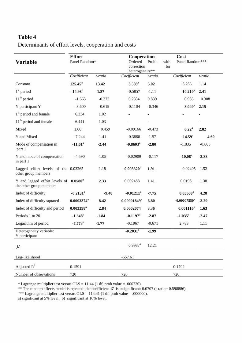
Table 4 Determinants of effort levels, cooperation and costs
Variable Effort
Panel Random* Cooperation
Ordered Probit with correction for heterogeneity**
Cost Panel Random***
Coefficient t-ratio Coefficient t-ratio Coefficient t-ratio
Constant 125.45a 13.42 3.539a 5.02 6.263 1.14
1st period - 14.98b -1.87 -0.5857 -1.11 10.210a 2.41
11th period -1.663 -0.272 0.2834 0.839 0.936 0.308
Y participant Y -3.600 -0.619 -0.1104 -0.346 8.040a 2.15
1st period and female 6.334 1.02 - - - -
11th period and female 6.441 1.03 - - - -
Mixed 1.66 0.459 -0.09166 -0.473 6.22a 2.82
Y and Mixed -7.244 -1.41 -0.3880 -1.57 -14.59a -4.69
Mode of compensation in part 1
-11.61a -2.44 -0.8603a -2.80 -1.835 -0.665
Y and mode of compensation in part 1
-4.590 -1.05 -0.02909 -0.117 -10.08a -3.88
Lagged effort levels of the other group members
0.03265 1.18 0.003320b 1.91 0.02405 1.52
Y and lagged effort levels of the other group members
0.0580a 2.33 0.002483 1.41 0.0195 1.38
Index of difficulty -0.2131a -9.48 -0.01211a -7.75 0.05508a 4.28
Index of difficulty squared 0.0003374a 8.42 0.00001849a 6.80 -0.00007550a -3.29
Index of difficulty and period 0.003398a 2.84 0.0002074 3.36 0.001116b 1.63
Periods 1 to 20 -1.348b -1.84 -0.1197a -2.87 -1.035a -2.47
Logarithm of period -7.773b -1.77 -0.1967 -0.671 2.783 1.11
Heterogeneity variable: Y participant
-0.2031a -1.99
1µ 0.9987a 12.21
Log-likelihood -657.61 Adjusted R2 0.1591 0.1792
Number of observations 720 720 720 * Lagrange multiplier test versus OLS = 11.44 (1 df, prob value = .000720). ** The random effects model is rejected: the coefficient σ is insignificant: 0.0707 (t-ratio= 0.598886). *** Lagrange multiplier test versus OLS = 114.41 (1 df, prob value = .000000). a) significant at 5% level; b) significant at 10% level.

Appendix A - Instructions
Instructions for X participants in the mixed-treatment – Part 1 You are going to participate in an experiment about incentives in work organization, which is part of a scientific program supported by your company and by the CNRS (French National Center for Scientific Research).
During this experimental session, you can earn money. The amount of your earnings depends not only on your decisions, but also on the decisions of the other participants with whom you will interact.
This session consists in 2 parts of 10 periods each. The session should last about one hour. During this session, transactions are conducted in ECU (Experimental Currency Units). Your final earnings are equal to the sum of the ECU you will earn in each of the 20 periods. At the end of the session, the total amount of ECU you have earned will be converted to Euros at the following rate: 10 ECU = 0.30 € In addition, you will receive a show-up fee of 7,60 €. Your entire earnings from the
experiment will be paid in vouchers that which will be given to you in a few days.
At the beginning of the session, the group of participants is subdivided into two categories: X and Y participants. You are an X participant. X or Y, you keep the same role throughout this session.
Periods 1-10 What does occur in each period? In each period, which lasts 1 minute, each participant has to perform a task on his or her
computer.
The task consists in uncovering a curve where a line has been plotted beforehand.
This curve is increasing and/or flat but it never decreases. It can have single or multiple peaks,
with a maximum of 3 peaks that are ranked from the lowest to the highest. The highest
altitude that can be reached by this curve is 100.
You uncover the line of this curve as you move along. Starting from the point 0, you are making progress at the same time in terms of distance (you are going along the horizontal axis) and in terms of altitude (you are going up on the vertical axis). Time starts running as soon as you click the “OK” button. You can move by clicking one of two buttons offered on your computer screen. These two buttons correspond to two available speeds.
� A first button enables you to take steps of 1. Steps of 1 do not cost money. � A second button enables you to take steps of 2. These steps are twice as rapid as steps of 1, but
each step of 2 costs 0.4 ECU. You may switch speed whenever you want and as many times as you like. As long as you do not want to change your speed, you can hold the mouse down and the progression along the curve automatically proceed at the chosen speed. You can stop your progression whenever you like, even before the one-minute time is over.
When a new period starts, you have to uncover a different curve.
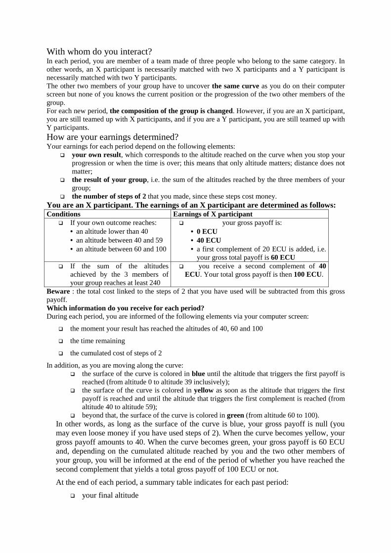
With whom do you interact? In each period, you are member of a team made of three people who belong to the same category. In other words, an X participant is necessarily matched with two X participants and a Y participant is necessarily matched with two Y participants. The other two members of your group have to uncover the same curve as you do on their computer screen but none of you knows the current position or the progression of the two other members of the group. For each new period, the composition of the group is changed. However, if you are an X participant, you are still teamed up with X participants, and if you are a Y participant, you are still teamed up with Y participants. How are your earnings determined? Your earnings for each period depend on the following elements:
� your own result, which corresponds to the altitude reached on the curve when you stop your progression or when the time is over; this means that only altitude matters; distance does not matter;
� the result of your group, i.e. the sum of the altitudes reached by the three members of your group;
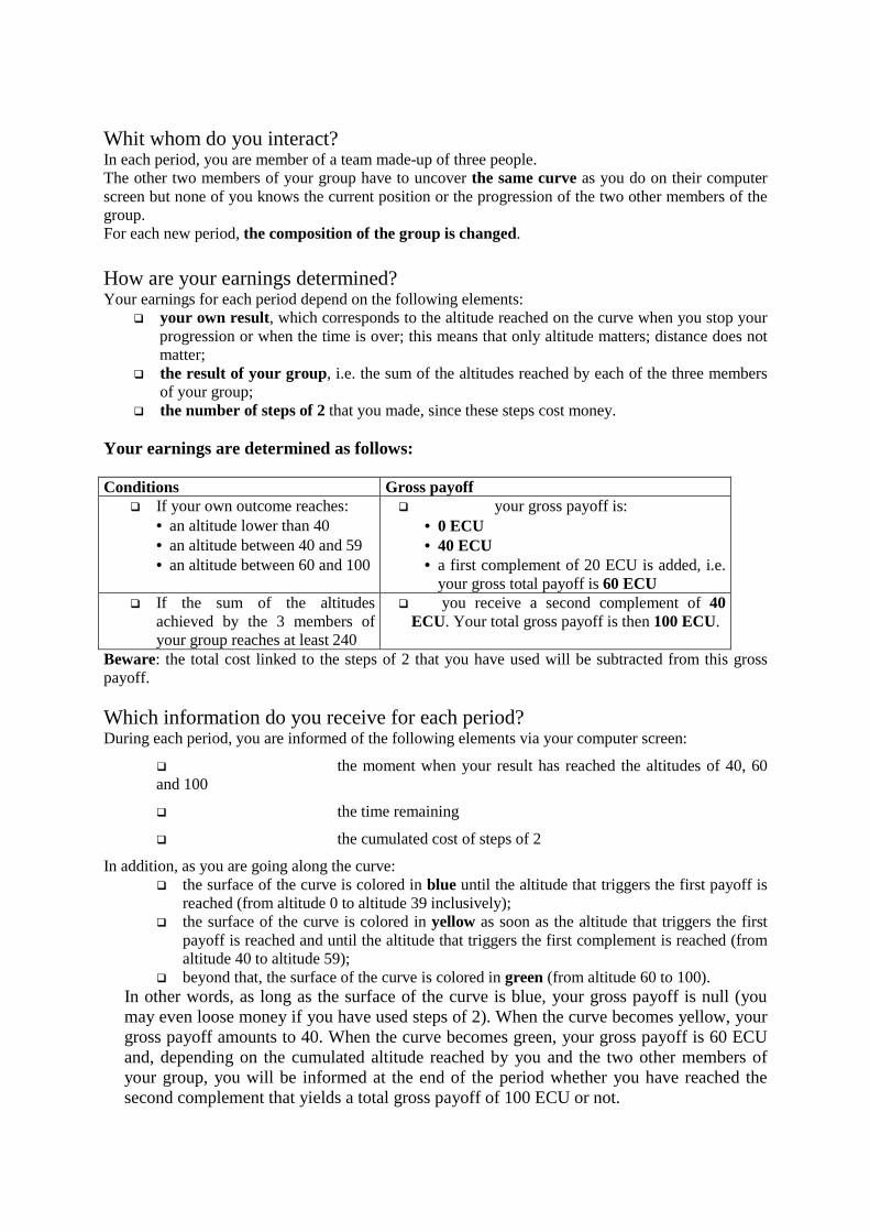
� the number of steps of 2 that you made, since these steps cost money. You are an X participant. The earnings of an X participant are determined as follows: Conditions Earnings of X participant
� If your own outcome reaches: • an altitude lower than 40 • an altitude between 40 and 59 • an altitude between 60 and 100
� your gross payoff is: • 0 ECU • 40 ECU • a first complement of 20 ECU is added, i.e.
your gross total payoff is 60 ECU � If the sum of the altitudes
achieved by the 3 members of your group reaches at least 240
� you receive a second complement of 40 ECU. Your total gross payoff is then 100 ECU.
Beware : the total cost linked to the steps of 2 that you have used will be subtracted from this gross payoff. Which information do you receive for each period? During each period, you are informed of the following elements via your computer screen:
� the moment your result has reached the altitudes of 40, 60 and 100
� the time remaining
� the cumulated cost of steps of 2
In addition, as you are moving along the curve: � the surface of the curve is colored in blue until the altitude that triggers the first payoff is
reached (from altitude 0 to altitude 39 inclusively); � the surface of the curve is colored in yellow as soon as the altitude that triggers the first
payoff is reached and until the altitude that triggers the first complement is reached (from altitude 40 to altitude 59);
� beyond that, the surface of the curve is colored in green (from altitude 60 to 100). In other words, as long as the surface of the curve is blue, your gross payoff is null (you may even loose money if you have used steps of 2). When the curve becomes yellow, your gross payoff amounts to 40. When the curve becomes green, your gross payoff is 60 ECU and, depending on the cumulated altitude reached by you and the two other members of your group, you will be informed at the end of the period of whether you have reached the second complement that yields a total gross payoff of 100 ECU or not.
At the end of each period, a summary table indicates for each past period:
� your final altitude
� the cumulated altitude of your group
� the total cost of steps of 2 that you used
� whether you have reached the first payoff of 40 ECU and the first complement of 20 ECU
� whether the cumulated result of your group enables you to get the second complement of 40 ECU
� your total net earnings. *** If you have any questions regarding these instructions, please raise your hand. Someone will answer your questions privately. Throughout the entire session, talking is not allowed. As soon as everybody is ready, we will begin with 3 practice periods, in order for you to
familiarize yourself with the task at hand. The results of these practice periods will not be
taken into account in your earnings.
Thank you for your participation.
***
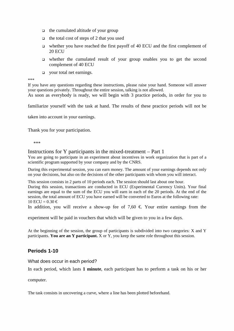
Instructions for Y participants in the mixed-treatment – Part 1 You are going to participate in an experiment about incentives in work organization that is part of a scientific program supported by your company and by the CNRS.
During this experimental session, you can earn money. The amount of your earnings depends not only on your decisions, but also on the decisions of the other participants with whom you will interact.
This session consists in 2 parts of 10 periods each. The session should last about one hour. During this session, transactions are conducted in ECU (Experimental Currency Units). Your final earnings are equal to the sum of the ECU you will earn in each of the 20 periods. At the end of the session, the total amount of ECU you have earned will be converted to Euros at the following rate: 10 ECU = 0.30 € In addition, you will receive a show-up fee of 7,60 €. Your entire earnings from the
experiment will be paid in vouchers that which will be given to you in a few days.
At the beginning of the session, the group of participants is subdivided into two categories: X and Y participants. You are an Y participant. X or Y, you keep the same role throughout this session.
Periods 1-10
What does occur in each period? In each period, which lasts 1 minute, each participant has to perform a task on his or her
computer.
The task consists in uncovering a curve, where a line has been plotted beforehand.

This curve is increasing and/or flat but it never decreases. It can have single or multiple peaks,
with a maximum of 3, which are ranked from the lowest to the highest. The highest altitude
that can be reached is 100 by this curve.
You uncover the line of this curve as you move along. Starting from the point 0, you are making progress at the same time in terms of distance (you are going along the horizontal axis) and in terms of altitude (you are going up on the vertical axis). Time starts running as soon as you click the “OK” button. You can move by clicking one of two buttons offered on your computer screen. These two buttons correspond to two available speeds.
� A first button enables you to take steps of 1. Steps of 1 do not cost money. � A second button enables you to take steps of 2. These steps are twice as rapid as steps of 1, but
each step of 2 costs 0.4 ECU. You may switch speed whenever you want and as many times as you like. As long as you do not want to change your speed, you can hold the mouse down and the progression along the curve automatically proceed at the chosen speed. You can stop your progression whenever you like, even before the one-minute time is over. When a new period starts, you have to uncover a different curve. With whom do you interact? In each period, you are member of a team made-up of three people who belong to the same
category. In other words, an X participant is necessarily matched with two X participants and
a Y participant is necessarily matched with two Y participants.
The other two members of your group have to uncover the same curve as you do on their computer screen but none of you knows the current position or the progression of the two other members of the group. For each new period, the composition of the group is changed. However, if you are a participant X, you are still teamed up with X participants, and if you are a Y participant, you are still teamed up with Y participants. How are your earnings determined? Your earnings for each period depend on the following elements:
� your own result, which corresponds to the altitude reached on the curve when you stop your progression or when the time is over; this means that only altitude matters; distance does not matter;
� the result of your group, i.e. the sum of the altitudes reached by each of the three members of your group;
� the number of steps of 2 that you made, since these steps cost money. You are an Y participant. The earnings of an Y participant are determined as follows: Conditions Earnings of Y participant
� If your own result reaches: • an altitude lower than 40 • an altitude between 40 and 100
� your gross payoff is: • 0 ECU • 60 ECU
� If the sum of the altitudes achieved by the 3 members of your group reaches at least 240
� you receive a complement of 40 ECU. Your total gross payoff is then 100 ECU.

Beware: the total cost linked to the steps of 2 that you have used will be subtracted from this gross payoff. Which information do you receive for each period? During each period, you are informed of the following elements via your computer screen:
� the moment your result has reached the altitudes of 40 and 100
� the time remaining
� the cumulated cost of steps of 2
In addition, as you are moving along the curve: � the surface of the curve is colored in blue until the altitude that triggers the first payoff is
reached (from altitude 0 to altitude 39 inclusively); � the surface of the curve is colored in yellow as soon as the altitude that triggers the first
payoff is reached (from altitude 40 to altitude 100). In other words, as long as the surface of the curve is blue, your gross payoff is null (you may even loose money if you have used steps of 2). When the curve becomes yellow, your gross payoff amounts to 60 and, depending on the cumulated altitude reached by you and the two other members of your group, you will be informed at the end of the period whether you have reached the complement that yields a total gross payoff of 100 ECU.
At the end of each period, a summary table indicates for each past period:
� your final altitude
� the cumulated altitude of your group
� the total cost of steps of 2 that you used
� whether you have reached the first payoff of 60 ECU
� whether the cumulated result of your group enables you to get the complement of 40 ECU
� your total net earnings. *** If you have any questions regarding these instructions, please raise your hand. Someone will answer your questions privately. Throughout the entire session, talking is not allowed. As soon as everybody is ready, we will begin with 3 practice periods, in order for you to
familiarize yourself with the task at hand. The results of these practice periods will not be
taken into account in your earnings. Thank you for your participation.
***
Instructions for both X and Y participants in the mixed-treatment – Part 2 Periods 11 – 20
We will now start with the second part of the experiment. The task has the same characteristics as in the first 10 periods. Information is the same as in part 1. At the start of a new period, the curve and the composition of the group are changed.
What is different from the preceding periods? Two elements have changed.
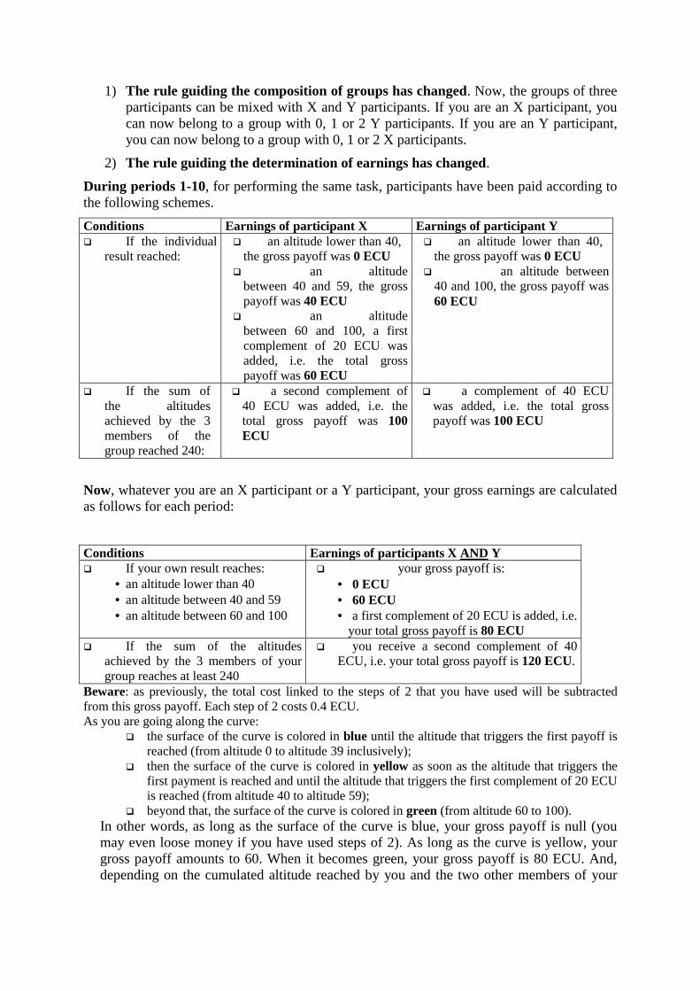
1) The rule guiding the composition of groups has changed. Now, the groups of three participants can be mixed with X and Y participants. If you are an X participant, you can now belong to a group with 0, 1 or 2 Y participants. If you are an Y participant, you can now belong to a group with 0, 1 or 2 X participants.
2) The rule guiding the determination of earnings has changed.
During periods 1-10, for performing the same task, participants have been paid according to the following schemes. Conditions Earnings of participant X Earnings of participant Y � If the individual
result reached:
� an altitude lower than 40, the gross payoff was 0 ECU
� an altitude between 40 and 59, the gross payoff was 40 ECU
� an altitude between 60 and 100, a first complement of 20 ECU was added, i.e. the total gross payoff was 60 ECU
� an altitude lower than 40, the gross payoff was 0 ECU
� an altitude between 40 and 100, the gross payoff was 60 ECU
� If the sum of the altitudes achieved by the 3 members of the group reached 240:
� a second complement of 40 ECU was added, i.e. the total gross payoff was 100 ECU
� a complement of 40 ECU was added, i.e. the total gross payoff was 100 ECU
Now, whatever you are an X participant or a Y participant, your gross earnings are calculated as follows for each period:
Conditions Earnings of participants X AND Y � If your own result reaches:
• an altitude lower than 40 • an altitude between 40 and 59 • an altitude between 60 and 100
� your gross payoff is: • 0 ECU • 60 ECU • a first complement of 20 ECU is added, i.e.
your total gross payoff is 80 ECU � If the sum of the altitudes
achieved by the 3 members of your group reaches at least 240
� you receive a second complement of 40 ECU, i.e. your total gross payoff is 120 ECU.
Beware: as previously, the total cost linked to the steps of 2 that you have used will be subtracted from this gross payoff. Each step of 2 costs 0.4 ECU. As you are going along the curve:
� the surface of the curve is colored in blue until the altitude that triggers the first payoff is reached (from altitude 0 to altitude 39 inclusively);
� then the surface of the curve is colored in yellow as soon as the altitude that triggers the first payment is reached and until the altitude that triggers the first complement of 20 ECU is reached (from altitude 40 to altitude 59);
� beyond that, the surface of the curve is colored in green (from altitude 60 to 100). In other words, as long as the surface of the curve is blue, your gross payoff is null (you may even loose money if you have used steps of 2). As long as the curve is yellow, your gross payoff amounts to 60. When it becomes green, your gross payoff is 80 ECU. And, depending on the cumulated altitude reached by you and the two other members of your
group, you will be informed at the end of the period whether you have reached the second complement that yields a total gross payoff of 120 ECU or not.
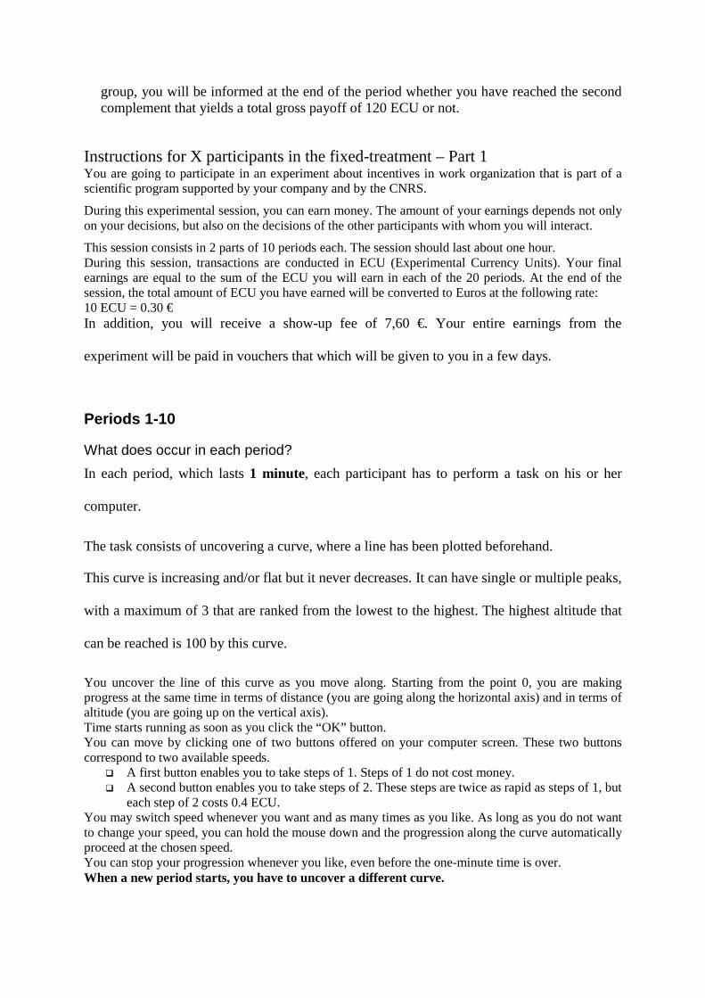
Instructions for X participants in the fixed-treatment – Part 1 You are going to participate in an experiment about incentives in work organization that is part of a scientific program supported by your company and by the CNRS.
During this experimental session, you can earn money. The amount of your earnings depends not only on your decisions, but also on the decisions of the other participants with whom you will interact.
This session consists in 2 parts of 10 periods each. The session should last about one hour. During this session, transactions are conducted in ECU (Experimental Currency Units). Your final earnings are equal to the sum of the ECU you will earn in each of the 20 periods. At the end of the session, the total amount of ECU you have earned will be converted to Euros at the following rate: 10 ECU = 0.30 € In addition, you will receive a show-up fee of 7,60 €. Your entire earnings from the
experiment will be paid in vouchers that which will be given to you in a few days.
Periods 1-10
What does occur in each period? In each period, which lasts 1 minute, each participant has to perform a task on his or her
computer.
The task consists of uncovering a curve, where a line has been plotted beforehand.
This curve is increasing and/or flat but it never decreases. It can have single or multiple peaks,
with a maximum of 3 that are ranked from the lowest to the highest. The highest altitude that
can be reached is 100 by this curve.
You uncover the line of this curve as you move along. Starting from the point 0, you are making progress at the same time in terms of distance (you are going along the horizontal axis) and in terms of altitude (you are going up on the vertical axis). Time starts running as soon as you click the “OK” button. You can move by clicking one of two buttons offered on your computer screen. These two buttons correspond to two available speeds.
� A first button enables you to take steps of 1. Steps of 1 do not cost money. � A second button enables you to take steps of 2. These steps are twice as rapid as steps of 1, but
each step of 2 costs 0.4 ECU. You may switch speed whenever you want and as many times as you like. As long as you do not want to change your speed, you can hold the mouse down and the progression along the curve automatically proceed at the chosen speed. You can stop your progression whenever you like, even before the one-minute time is over. When a new period starts, you have to uncover a different curve.
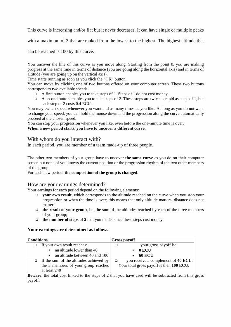
Whit whom do you interact? In each period, you are member of a team made-up of three people. The other two members of your group have to uncover the same curve as you do on their computer screen but none of you knows the current position or the progression of the two other members of the group. For each new period, the composition of the group is changed. How are your earnings determined? Your earnings for each period depend on the following elements:
� your own result, which corresponds to the altitude reached on the curve when you stop your progression or when the time is over; this means that only altitude matters; distance does not matter;
� the result of your group, i.e. the sum of the altitudes reached by each of the three members of your group;
� the number of steps of 2 that you made, since these steps cost money. Your earnings are determined as follows: Conditions Gross payoff
� If your own outcome reaches: • an altitude lower than 40 • an altitude between 40 and 59 • an altitude between 60 and 100
� your gross payoff is: • 0 ECU • 40 ECU • a first complement of 20 ECU is added, i.e.
your gross total payoff is 60 ECU � If the sum of the altitudes
achieved by the 3 members of your group reaches at least 240
� you receive a second complement of 40 ECU. Your total gross payoff is then 100 ECU.
Beware: the total cost linked to the steps of 2 that you have used will be subtracted from this gross payoff. Which information do you receive for each period? During each period, you are informed of the following elements via your computer screen:
� the moment when your result has reached the altitudes of 40, 60 and 100
� the time remaining
� the cumulated cost of steps of 2
In addition, as you are going along the curve: � the surface of the curve is colored in blue until the altitude that triggers the first payoff is
reached (from altitude 0 to altitude 39 inclusively); � the surface of the curve is colored in yellow as soon as the altitude that triggers the first
payoff is reached and until the altitude that triggers the first complement is reached (from altitude 40 to altitude 59);
� beyond that, the surface of the curve is colored in green (from altitude 60 to 100). In other words, as long as the surface of the curve is blue, your gross payoff is null (you may even loose money if you have used steps of 2). When the curve becomes yellow, your gross payoff amounts to 40. When the curve becomes green, your gross payoff is 60 ECU and, depending on the cumulated altitude reached by you and the two other members of your group, you will be informed at the end of the period whether you have reached the second complement that yields a total gross payoff of 100 ECU or not.
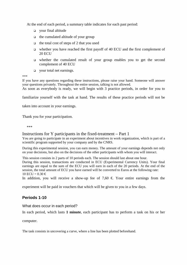
At the end of each period, a summary table indicates for each past period:
� your final altitude
� the cumulated altitude of your group
� the total cost of steps of 2 that you used
� whether you have reached the first payoff of 40 ECU and the first complement of 20 ECU
� whether the cumulated result of your group enables you to get the second complement of 40 ECU
� your total net earnings. *** If you have any questions regarding these instructions, please raise your hand. Someone will answer your questions privately. Throughout the entire session, talking is not allowed. As soon as everybody is ready, we will begin with 3 practice periods, in order for you to
familiarize yourself with the task at hand. The results of these practice periods will not be
taken into account in your earnings.
Thank you for your participation.
***
Instructions for Y participants in the fixed-treatment – Part 1 You are going to participate in an experiment about incentives in work organization, which is part of a scientific program supported by your company and by the CNRS.
During this experimental session, you can earn money. The amount of your earnings depends not only on your decisions, but also on the decisions of the other participants with whom you will interact.
This session consists in 2 parts of 10 periods each. The session should last about one hour. During this session, transactions are conducted in ECU (Experimental Currency Units). Your final earnings are equal to the sum of the ECU you will earn in each of the 20 periods. At the end of the session, the total amount of ECU you have earned will be converted to Euros at the following rate: 10 ECU = 0.30 € In addition, you will receive a show-up fee of 7,60 €. Your entire earnings from the
experiment will be paid in vouchers that which will be given to you in a few days.
Periods 1-10
What does occur in each period? In each period, which lasts 1 minute, each participant has to perform a task on his or her
computer.
The task consists in uncovering a curve, where a line has been plotted beforehand.
This curve is increasing and/or flat but it never decreases. It can have single or multiple peaks
with a maximum of 3 that are ranked from the lowest to the highest. The highest altitude that
can be reached is 100 by this curve.
You uncover the line of this curve as you move along. Starting from the point 0, you are making progress at the same time in terms of distance (you are going along the horizontal axis) and in terms of altitude (you are going up on the vertical axis). Time starts running as soon as you click the “OK” button. You can move by clicking one of two buttons offered on your computer screen. These two buttons correspond to two available speeds.
� A first button enables you to take steps of 1. Steps of 1 do not cost money. � A second button enables you to take steps of 2. These steps are twice as rapid as steps of 1, but
each step of 2 costs 0.4 ECU. You may switch speed whenever you want and as many times as you like. As long as you do not want to change your speed, you can hold the mouse down and the progression along the curve automatically proceed at the chosen speed. You can stop your progression whenever you like, even before the one-minute time is over. When a new period starts, you have to uncover a different curve. With whom do you interact with? In each period, you are member of a team made-up of three people.
The other two members of your group have to uncover the same curve as you do on their computer screen but none of you knows the current position or the progression rhythm of the two other members of the group. For each new period, the composition of the group is changed. How are your earnings determined? Your earnings for each period depend on the following elements:
� your own result, which corresponds to the altitude reached on the curve when you stop your progression or when the time is over; this means that only altitude matters; distance does not matter;
� the result of your group, i.e. the sum of the altitudes reached by each of the three members of your group;
� the number of steps of 2 that you made, since these steps cost money. Your earnings are determined as follows: Conditions Gross payoff
� If your own result reaches: • an altitude lower than 40 • an altitude between 40 and 100
� your gross payoff is: • 0 ECU • 60 ECU
� If the sum of the altitudes achieved by the 3 members of your group reaches at least 240
� you receive a complement of 40 ECU. Your total gross payoff is then 100 ECU.
Beware: the total cost linked to the steps of 2 that you have used will be subtracted from this gross payoff.
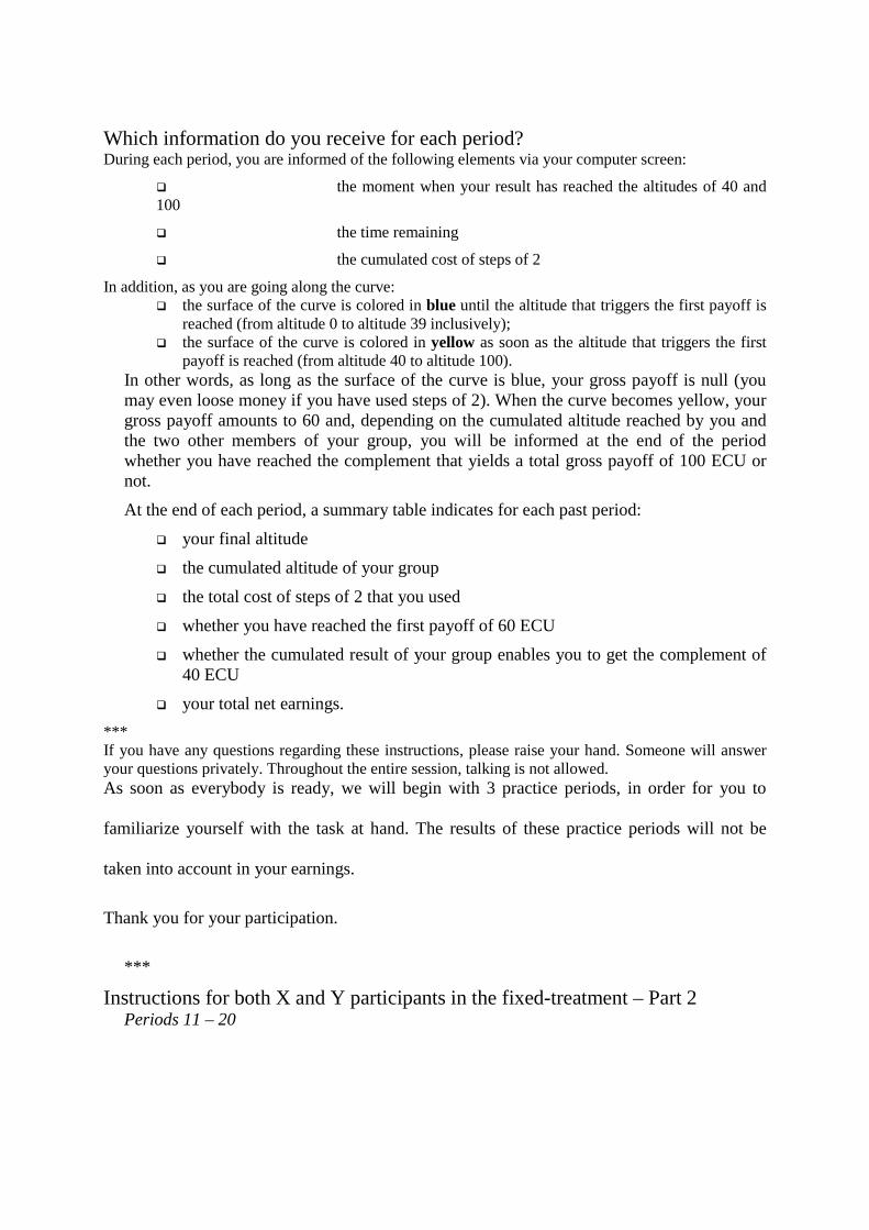
Which information do you receive for each period? During each period, you are informed of the following elements via your computer screen:
� the moment when your result has reached the altitudes of 40 and 100
� the time remaining
� the cumulated cost of steps of 2
In addition, as you are going along the curve: � the surface of the curve is colored in blue until the altitude that triggers the first payoff is
reached (from altitude 0 to altitude 39 inclusively); � the surface of the curve is colored in yellow as soon as the altitude that triggers the first
payoff is reached (from altitude 40 to altitude 100). In other words, as long as the surface of the curve is blue, your gross payoff is null (you may even loose money if you have used steps of 2). When the curve becomes yellow, your gross payoff amounts to 60 and, depending on the cumulated altitude reached by you and the two other members of your group, you will be informed at the end of the period whether you have reached the complement that yields a total gross payoff of 100 ECU or not.
At the end of each period, a summary table indicates for each past period:
� your final altitude
� the cumulated altitude of your group
� the total cost of steps of 2 that you used
� whether you have reached the first payoff of 60 ECU
� whether the cumulated result of your group enables you to get the complement of 40 ECU
� your total net earnings. *** If you have any questions regarding these instructions, please raise your hand. Someone will answer your questions privately. Throughout the entire session, talking is not allowed. As soon as everybody is ready, we will begin with 3 practice periods, in order for you to
familiarize yourself with the task at hand. The results of these practice periods will not be
taken into account in your earnings.
Thank you for your participation.
***
Instructions for both X and Y participants in the fixed-treatment – Part 2 Periods 11 – 20
We will now start with the second part of the experiment. The task has the same characteristics as in the first 10 periods. Information is the same as in part 1. At the start of a new period begins, the curve and the composition of the group are changed.
What is different from the preceding periods? Your gross earnings are now determined as follows for each period.
Conditions Gross payoff � If your own result reaches:
• an altitude lower than 40 • an altitude between 40 and 59 • an altitude between 60 and 100
� your gross payoff is: • 0 ECU • 60 ECU • a first complement of 20 ECU is added, i.e.
your total gross payoff is 80 ECU � If the sum of the altitudes
achieved by the 3 members of your group reaches at least 240
� you receive a second complement of 40 ECU, i.e. your total gross payoff is 120 ECU.
Beware: as previously, the total cost linked to the steps of 2 that you have used will be subtracted from this gross payoff. Each step of 2 still costs 0.4 ECU. As you are going along the curve:
� the surface of the curve is colored in blue until the altitude that triggers the first payoff is reached (from altitude 0 to altitude 39 inclusively);
� then the surface of the curve is colored in yellow as soon as the altitude that triggers the first payment is reached and until the altitude that triggers the first complement of 20 ECU is reached (from altitude 40 to altitude 59);
� beyond that, the surface of the curve is colored in green (from altitude 60 to 100). In other words, as long as the surface of the curve is blue, your gross payoff is null (you may even loose money if you have used steps of 2). As long as the curve is yellow, your gross payoff amounts to 60. When it becomes green, your gross payoff is 80 ECU. And, depending on the cumulated altitude reached by you and the two other members of your group, you will be informed at the end of the period whether you have reached the second complement that yields a total gross payoff of 120 ECU or not.