The response of the Red Sea to a strong wind jet

near the Tokar Gap in summer

By

Ping Zhai

B.S., Ocean University of China, 2006

M.S., Ocean University of China, 2008

Submitted in partial fulfillment of the requirements for the degree of

Master of Science

at the

MASSACHUSETTS INSTITUTE OF TECHNOLOGY

and the

WOODS HOLE OCEANOGRAPHIC INSTITUTION

September 2011 © Ping Zhai 2011. All rights reserved.

The author hereby grants to MIT and WHOI permission to reproduce and

to distribute publicly paper and electronic copies of this thesis document

in whole or in part in any medium now known or hereafter created.

Signature of Author _______________________________________________________________________________

Joint Program in Oceanography/Applied Ocean Science and Engineering Massachusetts Institute of Technology

and Woods Hole Oceanographic Institution July 21, 2011

Certified by _______________________________________________________________________________

Amy Bower, Senior Scientist Thesis Supervisor

Accepted by _______________________________________________________________________________

Karl R. Helfrich, Senior Scientist Chair, Joint Committee for Physical Oceanography

Massachusetts Institute of Technology/ Woods Hole Oceanographic Institution

The response of the Red Sea to a strong wind jet near the Tokar Gap in summer

By Ping Zhai

Submitted to the MIT/WHOI Joint Program in Physical Oceanography in

September 2011, in partial fulfillment of the requirements for the degree of

Master of Science

Abstract

Remote sensing and in situ observations are used to investigate the ocean response to the

Tokar Wind Jet in the Red Sea. The wind jet blows down the pressure gradient through the

Tokar Gap on the Sudanese coast, at about 18oN, during the summer monsoon season. It

disturbs the prevailing along-sea (southeastward) winds with strong cross-sea (northeastward)

winds that can last from days to weeks and reach amplitudes of 20-25 m/s. By comparing

scatterometer winds with along-track and gridded sea level anomaly observations, it is shown

that an intense dipolar eddy spins up in less than seven days in response to the wind jet. The

eddy pair has a horizontal scale of 140 km. Maximum ocean surface velocities can reach 1

m/s and eddy currents extend at least 200 m into the water column. The eddy currents appear

to cover the width of the sea, providing a pathway for rapid transport of marine organisms and

other drifting material from one coast to the other. Interannual variability in the strength of the

dipole is closely matched with variability in the strength of the wind jet. The dipole is

observed to be quasi-stationary, although there is some evidence for slow eastward

propagation—simulation of the dipole in an idealized high-resolution numerical model

suggests that this is the result of self-advection. These and other recent in situ observations in

the Red Sea show that the upper ocean currents are dominated by mesoscale eddies rather than

by a slow overturning circulation.

Thesis Supervisor:: Amy Bower

Title: Senior Scientist

Acknowledgements

I would like to thank the patient and stimulating support of my advisor, Amy Bower,

throughout this work. She is not only my advisor but also my mentor and friend. Thanks to

my committee members, Larry Pratt, Tom Farrar, Karl Helfrich and Glenn Flierl, for their

guidance and support to my thesis. Finally, I want to thank my parents and my brother. This

work is supported by Award Nos. USA 00002, KSA 00011 and KSA 00011/02 made by King

Abdullah University of Science and Technology (KAUST).

Contents Chapter 1: Introduction ....................................................................................................... 1

Chapter 2: Satellite observations of the wind jets near the Tokar Gap in the Red Sea .... 11

2.1 Data description ....................................................................................................... 11

2. 2 Seasonal variability of the wind near the Tokar Gap ............................................. 13

2.3 The interannual and daily variability of the Tokar Wind Jet .................................. 17

Chapter 3: The response of the Red Sea to the Tokar wind jet ......................................... 22

3.1 Data description-satellite SLA ................................................................................ 22

3.2 The dipole near the Tokar Gap in summer observed from satellite SLA ............... 25

3.3 The horizontal and vertical structure of the dipole ................................................. 37

Chapter 4: Idealized simulation using a 1.5-layer model ................................................. 44

4.1 The model description ............................................................................................. 44

4.2 The idealized simulation ......................................................................................... 46

Chapter 5: Conclusions and discussion ............................................................................. 55

Appendix: Dipole dynamics ............................................................................................. 57

Reference: ..................................................................................................... 63 

 

1  

Chapter 1: Introduction

The Red Sea is a long and narrow basin that is located between Africa and Asia (Figure 1.1).

It extends from 12.5oN to 30oN, a distance of about 2250 km, and is about 280km wide on

average. The average depth is about 490m, but a rift running down the axis is deeper than

2000m. The Red Sea is connected to the Indian Ocean through the strait of Bab el Mandeb,

and to the Mediterranean through the Suez Canal. At about 28oN, the Red Sea splits into the

Gulf of Suez and Gulf of Aqaba. At the southern end (about 12oN), the Red Sea has a

minimum width of 25km at the strait of Bab el Mandeb. At 13.7oN, slightly north of the strait

of Bab el Mandeb, there is a shallow sill with a greatest depth of 137m – Hanish Sill (Werner

and Lange, 1975).

Surrounded by extremely hot, dry deserts on all coasts, the Red Sea receives very little

precipitation. Due to high evaporation, negligible precipitation and lack of runoff supply, the

Red Sea is one of the most saline ocean basins in the world. Estimates of the evaporation rate

in the Red Sea have been obtained by using bulk formulae and the conservation of volume

and salt inside the Red Sea basin. Sofianos, et al (2002) review the previous estimates of the

evaporation-precipitation (E-P) rate in the Red Sea. The estimates range from 3.5m/year to

1.5m/year. Their estimate of the E-P rate over the Red Sea is 2.06±0.22m/year using the

conservation of the volume and salt in the Red Sea.

2  

Figure 1.1: A Red Sea topographic map. The colors are the elevation of the topography (unit:

m). The locations of Gulf of Aqaba (GAQ), Gulf of Suez (GS), Gulf of Aden (GA),

Mediterranean Sea (ME), Tokar Gap (TG), Strait of Bab el Mandeb (SBM) are shown. The

mean Sea Level Pressure (SLP) and 10-m wind in the box are shown in Figure 1.5.

Previous studies in the strait of Bab el Mandeb (e.g. Morcos, 1970; Maillard and Soliman,

1986; Patzert, 1974; Neuman and McGill, 1961; Murray and Johns, 1997) indicate a 2-layer

exchange flow pattern in winter and a 3-layer exchange flow pattern in summer, as shown in

Figure 1.2. In winter, the Red Sea Overflow Water (RSOW) flows out of the Red Sea with

salinity of 40psu beneath the incoming surface layer from the Gulf of Aden with salinity of

36.5psu. In summer, the exchange flow has a 3-layer structure: the surface flow from the Red

Sea, the incoming Gulf of Aden Intermediate Water and the outgoing RSOW. An 18-month

time series of moored ADCP and hydrographic observations of the exchange flow at the strait

of Bab el Mandeb was collected in 1995-1996 by Murray and Johns (1997). Velocity data

were collected at two sections: the narrowest section at Perim and the shallowest section at

Hanish. Their observations indicated that in winter (November to March) the average

3  

transport of RSOW is 0.6Sv with the speed of 0.8-1m/s. In summer (June to September), the

RSOW transport is reduced to 0.05Sv with a speed of 0.2-0.3m/s. Sofianos and Johns(2002)

studied the mechanism of the seasonal variation of the flow through the strait of Bab el

Mandeb by using the Miami Isopycnic Coordinate Ocean Model (MICOM). They argued that

the seasonal variation of the wind stress and the thermohaline forcing together form the

seasonal flow pattern at the strait.

Figure 1.2: Sketch of the two circulation patterns in the Bab el Mandeb. Left: winter, right:

Summer. SW=surface water, GAIW=Gulf of Aden intermediate water, RSOW=Red Sea

Overflow Water, SBM=Strait of Bab el Mandeb, GA=Gulf of Aden (reproduced from Smeed,

2004).

Wind and buoyancy forcing are two mechanisms that drive the Red Sea circulation. The

surface winds in the Red Sea are mainly along the axis of the basin due to the high mountain

ranges on both sides. Winds in the southern part are influenced by the Indian Monsoon. Figure

winter

southeastly

SW

RSOWGAIW

SBMRed Sea GA

summer

northwestly

GAIW

RSOW

SW

SBMRed Sea GA

4  

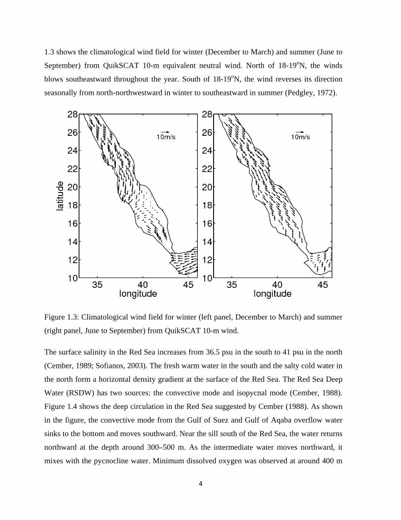
1.3 shows the climatological wind field for winter (December to March) and summer (June to

September) from QuikSCAT 10-m equivalent neutral wind. North of 18-19oN, the winds

blows southeastward throughout the year. South of 18-19oN, the wind reverses its direction

seasonally from north-northwestward in winter to southeastward in summer (Pedgley, 1972).

Figure 1.3: Climatological wind field for winter (left panel, December to March) and summer

(right panel, June to September) from QuikSCAT 10-m wind.

The surface salinity in the Red Sea increases from 36.5 psu in the south to 41 psu in the north

(Cember, 1989; Sofianos, 2003). The fresh warm water in the south and the salty cold water in

the north form a horizontal density gradient at the surface of the Red Sea. The Red Sea Deep

Water (RSDW) has two sources: the convective mode and isopycnal mode (Cember, 1988).

Figure 1.4 shows the deep circulation in the Red Sea suggested by Cember (1988). As shown

in the figure, the convective mode from the Gulf of Suez and Gulf of Aqaba overflow water

sinks to the bottom and moves southward. Near the sill south of the Red Sea, the water returns

northward at the depth around 300–500 m. As the intermediate water moves northward, it

mixes with the pycnocline water. Minimum dissolved oxygen was observed at around 400 m

5  

at the southern part of the Red Sea in summer 2001 (Sofianos, 2007, his Figure 5). At the

bottom near 27oN of the Red Sea, high dissolved oxygen concentration was also observed

which indicates the newly formed deep water. When the RSDW moves southward, the

dissolved oxygen is depleted and its concentration decreases. After the RSDW is uplifted near

Strait of Bab el Mandeb to around 400 m, it moves northward and mixes with the water from

upper layer. While it moves northward at around 400 m, its dissolved oxygen concentration

increases through mixing with the higher dissolved oxygen concentration water. The

isopycnal mode injects recently ventilated water just under the pycnocline, and gives rise to a

southward flow. Although there is no direct measurement of the intermediate northward return

flow, the distribution of Carbon-14 and 3He indicates its existence (Cember, 1988).

Tracer observations suggest that the Red Sea deep water masses can be separated into deep

and bottom water. The CFC-12 anomaly in the bottom water in the northern end of the Red

Sea is also observed in the Gulf of Aqaba, which suggests that the bottom water (below 900 m

depth) is mainly formed by the Gulf of Aqaba outflow water. The deep water that is between

the bottom water and the intermediate water is found to be mainly from the Gulf of Suez

(Plahn et al., 2002).

6  

Figure 1.4: Schematic of the general circulation for the Red Sea Deep Water according to

Cember (1988). The red and blue arrows are convective mode and isopycnal mode

respectively.

Although most studies of Red Sea circulation have focused on the large scale overturning,

some observational and modeling studies have shown that eddies play an important part in the

horizontal circulation of the Red Sea. Morcos (1970) showed surface circulations inferred

from temperature and salinity observations taken during 1895-1896 and 1897-1898. The

studies showed a generally cyclonic circulation with a superimposed, but unresolved, eddy

field. Morcos and Soliman (1972) depicted a series of mainly cyclonic eddies and an

anticyclone centered near 23oN. The hydrographic surveys during the period from 1982 to

1987 reveal that the circulation of the Red Sea is composed of a series of gyres (Quadfasel

and Baudner, 1993). The cyclonic and anticyclonic gyres are not permanent, but tend to

reappear at preferential locations, like the anticyclone centered at 23oN and the cyclone near

26oN. The distribution of chlorophyll-a from SeaWiFS indicates an anticyclone centered at

23oN in August 1998 and an anticyclone centered at 18.7oN in October 2002 (Acker et al,

2007). Their results show that the ocean color data can provide information about the surface

circulation in the Red Sea, and the circulation can influence the distribution of chlorophyll-a.

Sofianos and Johns (2007) demonstrate by using shipboard ADCP data from an along-axis

7  

cruise track that there is a strong dipole near 19oN with a cyclone in the north and an

anticyclone in the south.

The formation mechanisms for the eddies in the Red Sea are still uncertain. Clifford et al.

(1997) pointed out that the formation of eddies in the Red Sea strongly depends on the wind

direction. They proposed that there would be more eddies in the Red Sea when the wind has a

cross-basin component. Pedgley (1972) shows a gap in the high orography on the west coast

of the Red Sea near 18oN, which is called Tokar Gap. Jiang et al. (2009) also point out that

there are a series of mountain gaps along both sides of the Red Sea that can at times cause

strong zonal wind jets to blow across the Red Sea. For example, in summer, there is a strong

wind jet blowing out of the Tokar Gap onto the Red Sea (Hickey and Goudie, 2007). In winter,

the wind jet near Tokar Gap reverses its direction and blows from the Red Sea into the Tokar

Gap (Pedgley, 1974, his Figure 1). Figure 1.5 shows the mean sea level pressure (SLP) and

10-m sea surface wind in August and December 2001 in the vicinity of the Tokar Gap. In

August, the SLP on the African coast is higher than in the Red Sea, and the wind blows down

the pressure gradient towards the Red Sea as a gravity flow through the Tokar Gap. The width

of the wind jet, which is 150-400km, is much smaller than the first baroclinic Rossby radius

of deformation for the atmosphere (approximately 1000km). The curvature of the path of the

wind jet is approximately equal to the inertial radius U/f (Pratt, et al., unpublished paper).

These suggest that the geostrophic balance is questionable in this area in summer. The

resolution of the SLP data used here is 1o, there might be some finer scales of geostrophic

adjustment process than SLP maps suggest. In December, the wind converges into the Tokar

Gap, and is almost along the isobars which implies that the wind in winter might be

geostrophically balanced in this region. To distinguish the different mechanisms of the winter

and summer winds near the Tokar Gap, the wind in winter is called “convergent wind”, and

the strong wind in summer is called Tokar Wind Jet.

8  

Figure 1.5: Mean SLP (contour) and 10m wind in January (upper panel) and August (lower

panel) 2001. SLP is from NCEP FNL Operational Model Global Tropospheric Analyses; 10-

m wind is from QuikSCAT; the colors are topography from etopo05.

Among the most studied wind jets blowing over the coastal ocean are the Tehuantepec,

Papagayo and Panama wind jets in Central America. The three mountain gaps that form the

9  

jets are shown in Figure 1.6. Together with the lower sea level pressure in the eastern Pacific,

strong wind jets are generated that blow into the eastern Pacific. During the wind jet events,

anticyclonic and cyclonic eddies are generated on the two sides of the wind jets (McCreary et

al., 1989) due to local wind stress curl and Ekman pumping. These authors studied the

dynamics of the evolution of the dipole using a 1.5-layer linear model and a 1.5-layer

nonlinear model with entrainment of cool water into the upper layer. The model results

indicate that the dipole propagates westward at a speed of the free linear Rossby wave speed

due to the effect. The wind jet studied in McCreary’s paper blows southward, therefore, the

self-propagation of the dipole, which would be southward, doesn’t have much impact on the

westward speed. Different from this case, the dipole near the Tokar gap has zonal self-

propagation speed since the Tokar wind jet has a zonal component. It is therefore anticipated

that self-propagation may influence the zonal movement of the Tokar dipole.

Figure 1.6: Topography of Central America; the arrows show the location of the three

mountain gaps.

10  

The previous observations and model work indicate that the eddies contribute to the main

circulation pattern of the Red Sea and the formation of the Red Sea water masses, such as the

formation of the deep water near the Gulf of Suez where there is a cyclonic gyre. The cyclonic

gyre is usually associated with thermocline uplift, which might enhance the vertical mixing

and cause the ventilation of the thermocline. Eddies in the Red Sea may have important

impacts on biological productivity and distributions. Thermocline uplift in the center of the

cyclonic eddy may bring the cold water and nutrients from the deep water to the surface layer

of the Red Sea, which is generally oligotrophic. This could increase the productivity in that

region. In addition, the eddies may transport nutrients from the coastal coral reefs into the

interior of the Red Sea. In October 2002, a low chl-a region centered along 18.5oN appeared

where there was an anticyclonic gyre (Acker, 2008, Fig. 8). The eddies in the Red Sea appear

to extend from one side of the Red Sea to the other side, which enhances the interaction and

communication of the two coasts of the Red Sea. For example, with the speed of 1m/s, a

particle can travel from the west coast to the east coast in 2-3 days. Therefore, it is important

to understand more about the eddies in the Red Sea. In this work, the structure, evolution and

dynamics of the dipole near the Tokar Gap will be studied, with the help of the satellite Sea

Level Anomaly (SLA), the QuikSCAT wind, in situ observations and a 1.5-layer model.

The remainder of this thesis is organized as follows. In Chapter 2, measurements of near sea-

surface winds by QuikSCAT from July 1999 to November 2009 are analyzed to investigate

the seasonal and interannual variability of the wind near the Tokar Gap. The response of the

Red Sea to the Tokar Wind Jet in summer is described in Chapter 3 using the satellite SLA

and in situ observations from ADCP and CTD. In Chapter 4, a 1.5-layer model is employed to

study the water movement forced by an idealized zonal wind jet. The influence of the

effect is examined. Chapter 5 contains conclusions and a discussion of the study.

11  

Chapter 2: Satellite observations of the wind jets near the Tokar Gap in the Red Sea

2.1 Data description

The QuikSCAT winds analyzed here are produced by Remote Sensing Systems and sponsored

by the NASA Ocean Vector Winds Science Team (Data used here are downloaded from

ftp://ftp.ssmi.com/qscat/). They were calculated using the QSCAT-1 model function

(SeaWinds on QuikSCAT Level 3 Daily, Gridded Ocean Winds Vectors, Guide Document,

2001). QuikSCAT data products include daily and time averaged wind data (3-day average,

weekly and monthly) at 10 m above the sea surface. The data products used here are 0.25-

degree gridded data. The daily data is divided into 2 maps based on ascending and descending

passes.

The wind stress yx , can be calculated from wind speed yx WW , by

smW

smWW

W

C

WWWWC

D

yxyxDayx

/25 10115.2

/25 11m/s 10)065.049.0(

11m/s 102.1

),(),(

3

3

3

22

, (2.1)

where 3/2.1 mkga is the air density, 22 yx WWW

is wind speed, DC is the neutral

stability drag coefficient developed by Large and Pond (1981). Hellerman and Rosenstein

(1983) approximated the drag coefficient by an polynomial including air-sea temperature

difference and wind velocity by

)(10214.0)(1012.010616.0

)(10868.010788.010934.0

5252

6

443

sasa

saD

TTWTTW

TTWC

, (2.2)

where aT and sT are air and sea temperatures respectively. Another algorithm that is used for

calculating drag coefficient is the Coupled Ocean–Atmosphere Response Experiment

12  

(COARE) bulk air-sea flux algorithm which includes the influences of wind speed, air-sea

temperature difference, moisture and surface gravity wave (Fairall et al. 2003). In this study,

the QuikSCAT wind stress is calculated from equation 2.1.

The QuikSCAT scatterometer measured winds between 3 and 30m/s with an accuracy of

2m/s in speed and 20o in direction. QuikSCAT winds and in-situ wind observations generally

compare well, even in the near shore regions. Satheesan et al. (2007) compared the

QuikSCAT winds with winds obtained from moored buoys at 8 locations over the Indian

Ocean. They concluded that the mean differences for wind speed and wind directions were

0.37m/s and 5.8o , with root mean square deviations of 1.57m/s and 44.1o. Pickett et al. (2003)

assessed the accuracy of QuikSCAT winds by comparing the QuikSCAT winds to the winds

from 12 nearshore U.S. West Coast buoys. The root-mean-squared differences were 1.4m/s

for speed and 37o for direction.

Beginning in September 2008, the Woods Hole Oceanographic Institution began work with

King Abdullah University of Science and Technology (KAUST) to maintain a fully-

instrumented surface mooring in the eastern Red Sea. The first KAUST-UOP buoy was

deployed on October 11, 2008 at 22.16oN, 38.50oE in about 700 m of water. The wind data

were collected from October 11, 2008 to November 20, 2009. The QuikSCAT wind used to

compare with the buoy winds is daily QuikSCAT swath data (twice a day, ascending and

descending passes), and is interpolated to the buoy location. The hourly buoy winds are

interpolated to the QuikSCAT wind time. Only wind speeds greater than 3m/s are considered.

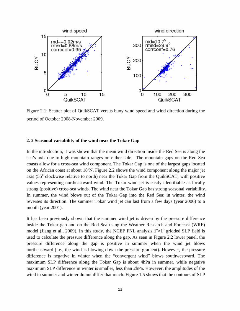
The scatter plots of the QuikSCAT versus buoy wind speeds and directions (Figure 2.1)

indicate that QuikSCAT captures the wind speed better than the wind direction. The statistical

analysis reveals that the linear correlation coefficient is 0.95 for the wind speed with a mean

difference and root mean squared difference of 0.02m/s and 0.68m/s, respectively. On the

other hand, for the wind direction, the linear correlation coefficient is 0.76 with a mean

difference and root mean squared difference of 10.7o and 29.9o. These statistical differences

are comparable to those found at other sites (see references above), confirming that the

QuikSCAT winds are reliable in the Red Sea.

13  

Figure 2.1: Scatter plot of QuikSCAT versus buoy wind speed and wind direction during the

period of October 2008-November 2009.

2. 2 Seasonal variability of the wind near the Tokar Gap

In the introduction, it was shown that the mean wind direction inside the Red Sea is along the sea’s axis due to high mountain ranges on either side. The mountain gaps on the Red Sea coasts allow for a cross-sea wind component. The Tokar Gap is one of the largest gaps located on the African coast at about 18oN. Figure 2.2 shows the wind component along the major jet axis (55o clockwise relative to north) near the Tokar Gap from the QuikSCAT, with positive values representing northeastward wind. The Tokar wind jet is easily identifiable as locally strong (positive) cross-sea winds. The wind near the Tokar Gap has strong seasonal variability. In summer, the wind blows out of the Tokar Gap into the Red Sea; in winter, the wind reverses its direction. The summer Tokar wind jet can last from a few days (year 2006) to a month (year 2001).

It has been previously shown that the summer wind jet is driven by the pressure difference inside the Tokar gap and on the Red Sea using the Weather Research and Forecast (WRF) model (Jiang et al., 2009). In this study, the NCEP FNL analysis 1o×1o gridded SLP field is used to calculate the pressure difference along the gap. As seen in Figure 2.2 lower panel, the pressure difference along the gap is positive in summer when the wind jet blows northeastward (i.e., the wind is blowing down the pressure gradient). However, the pressure difference is negative in winter when the “convergent wind” blows southwestward. The maximum SLP difference along the Tokar Gap is about 4hPa in summer, while negative maximum SLP difference in winter is smaller, less than 2hPa. However, the amplitudes of the wind in summer and winter do not differ that much. Figure 1.5 shows that the contours of SLP

14  

are more closely spaced in summer than in winter. The pressure gradient generates strong wind blowing into the Red Sea. Away from the coast, at a distance of approximately 100km, the wind jet turns clockwise. The anticyclonic turning of the Tokar wind jet might be due to the NNW prevailing wind in the Red Sea in summer. In winter, the NNW wind north of the Tokar Gap, and the SSE wind in the south converge into the Tokar Gap. The wind is almost parallel to the isobars with high SLP on the right-hand side, which indicates that the wind inside the Red Sea is mainly geostrophically balanced. The geostrophic wind speed is about 8m/s according to the SLP distribution near the Tokar Gap. Therefore, the mechanisms of the wind near the Tokar Gap in summer and winter might be different. The summer wind jet might be directly driven by the pressure gradient while the winter “convergent wind” might be mostly geostrophically balanced.

Figure 2.2: Upper panel: time series of the 10-m wind component along the major Tokar Wind Jet axis, which is 55o clockwise relative to the north. The wind is averaged in the box shown in the lower panel of Figure 1.5. Lower panel: time series of the 1o-gridded NCEP FNL SLP difference along the gap (SLPC-SLPB). The location of the two points are shown in Figure 1.5.

The seasonal variability of the Tokar Wind Jet is influenced by the Indian Monsoon. The Indian Monsoon winds blow northeastward during summer and southwestward during winter. The Indian Monsoon is related to the location of the InterTropical Convergence Zone (ITCZ), which is characterized by low SLP and heavy rainfall. The Indian summer monsoon generally occurs from June through September. Jiang et al. (2009) showed that ITCZ is between 15 –20oN in July and August on African (his Figure S2). The ITCZ can move as far north as 20oN

15  

during this time of year. Around September, the low SLP region moves southward as the ITCZ starts to move southward. Figure 2.3 is the SLP from NCEP FNL analysis data in January and August 2001. It shows that in summer, low SLP forms in Qinghai-Tibet Plateau and east Saudi Arabia which drives the southwest Indian summer monsoon. In winter, the low SLP in this region is replaced by high SLP and the wind reverses its direction in the Indian Ocean.

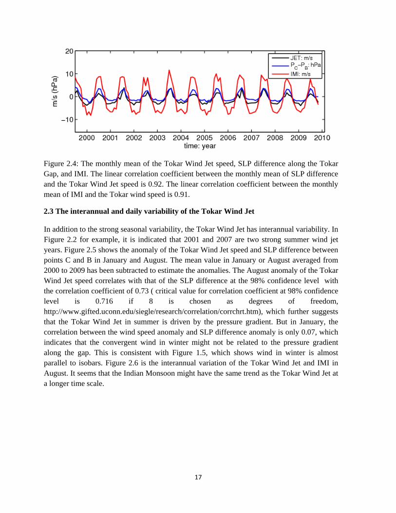
The Indian Monsoon Index(IMI) is defined using the difference of the 850-hPa zonal winds between a southern region of 5o–15 o N, 40 o –80 o E and a northern region of 20 o –30 o N, 70 o –90 o E (Figure 2.3) (Wang, et al., 2001). The IMI is used here to quantify the intensity of the Indian summer monsoon. Figure 2.4 shows the monthly mean of IMI, the Tokar wind and the SLP difference along the gap from 1999 to 2009. It suggests that the seasonal cycle of the Tokar wind is correlated with the Indian Monsoon Index with a correlation coefficient of 0.91. The lagged correlations (not shown here) between the Indian Monsoon and the Tokar wind speed indicate that on average, the Indian Monsoon is leading the Tokar wind by 8 days.

16  

Figure 2.3: Mean SLP (hPa) from NCEP FNL in January (upper panel) and August (lower panel) 2001. SLP is the theoretical pressure the air would have if the atmosphere continued below the ground to zero elevation (sea level). Low pressure areas form in the Qinghai-Tibet Plateau and east Saudi Arabia during the summer Indian Monsoon season. The zonal winds at 850hPa in boxes 1 and 2 are used to define the Indian Monsoon Index (IMI=U850(1)-U850(2)).

17  

Figure 2.4: The monthly mean of the Tokar Wind Jet speed, SLP difference along the Tokar Gap, and IMI. The linear correlation coefficient between the monthly mean of SLP difference and the Tokar Wind Jet speed is 0.92. The linear correlation coefficient between the monthly mean of IMI and the Tokar wind speed is 0.91.

2.3 The interannual and daily variability of the Tokar Wind Jet

In addition to the strong seasonal variability, the Tokar Wind Jet has interannual variability. In Figure 2.2 for example, it is indicated that 2001 and 2007 are two strong summer wind jet years. Figure 2.5 shows the anomaly of the Tokar Wind Jet speed and SLP difference between points C and B in January and August. The mean value in January or August averaged from 2000 to 2009 has been subtracted to estimate the anomalies. The August anomaly of the Tokar Wind Jet speed correlates with that of the SLP difference at the 98% confidence level with the correlation coefficient of 0.73 ( critical value for correlation coefficient at 98% confidence level is 0.716 if 8 is chosen as degrees of freedom, http://www.gifted.uconn.edu/siegle/research/correlation/corrchrt.htm), which further suggests that the Tokar Wind Jet in summer is driven by the pressure gradient. But in January, the correlation between the wind speed anomaly and SLP difference anomaly is only 0.07, which indicates that the convergent wind in winter might not be related to the pressure gradient along the gap. This is consistent with Figure 1.5, which shows wind in winter is almost parallel to isobars. Figure 2.6 is the interannual variation of the Tokar Wind Jet and IMI in August. It seems that the Indian Monsoon might have the same trend as the Tokar Wind Jet at a longer time scale.

18  

Figure 2.5: Anomaly of the Tokar wind speed and PC-PB for January (upper panel) and August (lower panel).

Figure 2.6: August Anomalies of the Tokar Wind Jet speed and IMI from 2000 to 2009. They

are correlated only at the 85% confidence level, if 8 is chosen as the degrees of freedom.

Based on results from an application of the Weather Research and Forecasting (WRF) model to the Red Sea region, which is initialized daily with 1o NCEP FNL, Jiang et al. (2009)

19  

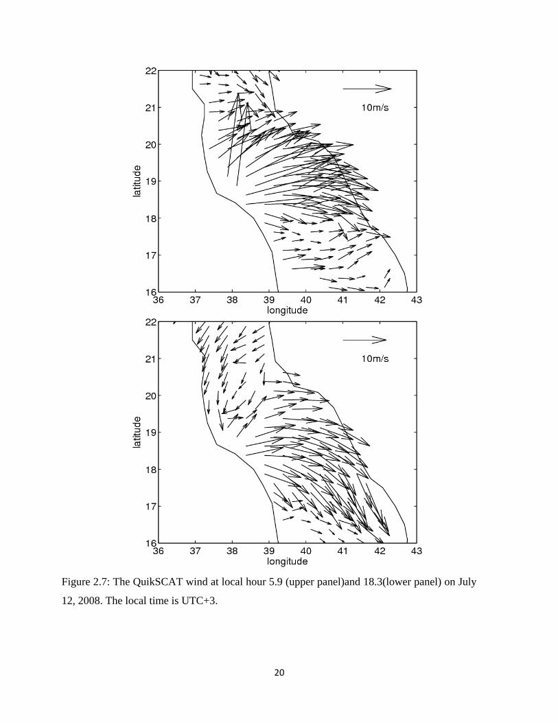
concluded that the Tokar Wind Jet has strong diurnal variability due to the opposite cross-shore temperature contrast during the day (generating westward sea breezes) and at night (generating eastward land breezes). Therefore, the summer Tokar Wind Jet is stronger in the early morning than in the evening during the summer. The strong diurnal variability of the wind jet is also demonstrated in QuikSCAT daily winds. Figure 2.7 shows the 10-m surface wind at local hours 5.9 and 18.3 on July 12, 2008. In the morning, the magnitude of wind stress is about 18m/s, while in the evening the magnitude is less than 10m/s. Figure 2.8 shows the time series of the offshore wind speed from QuikSCAT daily winds near the Tokar Gap in August 2001 and 2008, which indicates the daily cycle of the Tokar Wind Jet.

The summer Tokar Wind Jet has been reported occasionally by previous studies. With the help of the 10-year QuikSCAT wind, this chapter analyzed the annual, interannual and daily variability of the Tokar Wind Jet. The Tokar Wind Jet strength is correlated with the pressure difference along the Tokar Gap. It is clear that the seasonal variability of the Tokar Wind Jet is related to the Indian Monsoon. However, there are still some remaining questions. For example, is there a large-scale atmospheric mode of variability that influences the interannual variability of the SLP pressure difference, and thus the wind jet strength; or is the interannual variability of the wind jet a local phenomenon?

20  

Figure 2.7: The QuikSCAT wind at local hour 5.9 (upper panel)and 18.3(lower panel) on July

12, 2008. The local time is UTC+3.

21  

Figure 2.8: Time series of offshore wind speed from QuikSCAT daily winds near the Tokar

Gap averaged in the box in Figure 1.5. The offshore direction is 55o clockwise relative to the

north.

22  

Chapter 3: The response of the Red Sea to the Tokar wind jet

3.1 Data description-satellite SLA

Satellite altimetry can measure the Sea Surface Height (SSH). Mesoscale eddies in the ocean

can be detected by their Sea Level Anomaly (SLA). The satellite SLA data used here is

computed with respect to the CLS01 mean sea surface height (CLS01 MSS). The CLS01 MSS

is computed from 7 years of Topex/Poseidon mean profile (1993- 1999), 5 years of ERS-1/2

mean profile (1993-1999), 2 years of Geosat mean profile (1987-1988) and ERS-1 geodetic

data (Hernandez and Schaeffer 2001).

Because of the geostrophic balance, the center of a cyclonic eddy has a low sea level and the

center of an anticyclonic eddy has a high sea level (in the Northern Hemisphere). For example,

at latitude 20oN, with a velocity of 0.5m/s and radius 100km, the sea level difference between

the edge and the center of the eddy is about 25cm.

The satellite TOPEX/Poseidon was launched on 10 August 1992. It measured the sea surface

height every 10 days with an rms accuracy of 5cm (Fu, et al 1994). In the following years,

several other altimetry satellites were launched. The repeat periods of GFO, ERS-1/2, Jason-

1/2 and Envisat are 17, 35, 10 and 35 days, respectively. Figure 3.1 shows the repeat GFO

tracks over the Red Sea. Track-227 extends from the north of the Red Sea to 16oN. The

distance between two measurement points along each track is about 6.7km. Combining the

data of all available satellites, AVISO provides the merged SLA

(http://www.aviso.oceanobs.com/en/data/data-access-services/opendap/opendap-sla-

products/index.html), which is mapped on a regular 0.25o grid every 7 days. The resolution of

the gridded SLA is 2o in latitude and longitude. The merged SLA data have lower mapping

errors and better spatial coverage than would data from one satellite alone (Ducet et al., 2000).

It is important to point out that the data used here are anomalies since the Mean Dynamic

Topography (MDT) is unknown in the Red Sea. The Mean Sea Surface (MSS) includes the

geoid and the sea elevation. The MDT is related to the mean oceanic circulation and doesn’t

include the geoid.

23  

Figure 3.1: GFO 17-day repeat tracks inside the Red Sea with pass numbers given for each

track.

The satellite along-track and gridded SLA have been used previously to reveal some features

of sea level variability in the Red Sea. Cromwell and Smeed (1998) analyzed SLA at (41oE,

17.3oN) and (42oE, 15oN) from 1992 to 1997, and pointed out that the SLA in the southern

Red Sea has an annual cycle with amplitude of 18cm and reaches a maximum in winter. They

found that the wind forcing is the main reason for the SLA annual cycle by analysis of the

coherence between wind stress and SLA. Sofianos and Johns (2001) confirmed this relation

between the seasonal variation of SLA and the wind by using a model that balances the sea

level and the wind stress . They also found that the steric effect has a larger impact in the

southern Red Sea due to the intrusion of the cold Gulf of Aden Water than in the northern Red

Sea.

In addition to the annual cycle in SLA, which is illustrated for one location in the central Red

Sea by the dashed line in Figure 3.2, the SLA has a persistent monthly variation (Figure 3.2)

24  

with an amplitude of about 5cm. The altimetry satellites have different repeat periods, so the

number of satellite tracks that pass the Red Sea during a seven-day period varies with time.

However, comparison between the SLA and the satellite tracks passing the Red Sea reveals

that the monthly variation of SLA is not due to the different repeating periods of satellites.

Further evidence that the monthly signal is not due to uneven sampling by the altimeters is

provided by the steric height calculated from the mooring data. The mooring was deployed on

11 October 2008 at approximately 22.16°N, 38.5°E and collects accurate time series of

surface meteorology and upper ocean temperatures, velocities and salinities. The steric height

has the similar monthly variation as the SLA (Figure 3.2). Although the annual cycle of the

SLA and the steric height is different, the monthly variation of SLA and steric height agrees

well with each other. The reason for the monthly variation of the SLA and steric height is not

clear yet. In summer, the water is warmer and the water column is expanded. Therefore, the

steric height is larger in summer than in winter. The wind direction in the southern part of the

Red Sea has an direct impact on the sea surface height in the Red Sea. In summer, the wind

blows southeastward, which moves the water out of the Red Sea and decreases the sea surface

height. However, in winter, the wind in the southern Red Sea reverses its direction and moves

the water into the Red Sea. So it might be the annual cycle of the wind direction in the

southern part of the Red Sea that causes the annual variation of the sea surface height in the

Red Sea.

25  

Figure 3.2: Time series of SLA (22.25oN,38.5oE) and steric height (22.16oN, 38.5oE). The

steric height is calculated from the mooring salinity and temperature profiles with the

reference level at 200 m.

3.2 The dipole near the Tokar Gap in summer observed from satellite SLA

The satellite altimetry reveals that there are many eddies in the Red Sea throughout the year,

that often appear in pairs. The most obvious pair of eddies exists near the Tokar Gap at 18oN

in July and/or August. Figure 3.3 shows the SLA averaged in August 2001. It shows that north

of 18oN, there is a low SLA center, and south of 18oN, there is a high SLA center. Since the

mean dynamic topography is unknown for the Red Sea, only the surface geostrophic current

anomaly (eddy geostrophic current) can be calculated. Equation (3.1)

26  

y

u

x

v

xf

gv

yf

gu

, (3.1)

where is SLA, f is the Coriolis parameter, g is gravity and is relative vorticity, shows

how geostrophic current and the relative vorticity are calculated. In the calculation, the central

difference is applied in the middle region and backward or forward difference is applied on

the boundaries. In Figure 3.3, two eddies near 18oN rotate in opposite directions. These two

eddies of approximately 70km in radius have basin wide scale. The gridded SLA product,

which has some inherent spatial smoothing, may smear small-scale features.

27  

Figure 3.3: Upper panel: mean SLA (unit: cm) in August 2001; lower panel: the mean surface

geostrophic current anomaly calculated from the SLA and the relative vorticity (unit: 10-6s-1)

in August 2001.

28  

Figure 3.4 shows the velocity measured on August 13, 2001 at 22m depth, obtained with a

hull-mounted Acoustic Doppler Current Profiler (ADCP) (Sofianos and Johns, 2007). The

geostrophic surface current anomaly calculated from GFO along-track SLA on August 17,

2001 agrees well with the in situ observations both in direction and in magnitude, which

indicates that the along-track satellite data is reliable for studying the dipole. The velocity

observations from the ADCP and along-track SLA show that azimuthal speeds of the dipole

can reach 1m/s. The geostrophic velocity calculated from the gridded merged SLA typically

has a smaller magnitude than that from the along track SLA (Figure 3.5). Ducet, et al. (2000)

pointed out that the merged data underestimates the variability and is weaker than the along-

track data. The resolution of the gridded merged SLA is about 2o in the Red Sea (Ducet et al,

2000), which almost covers the whole width of the basin. Although the merged product

underestimates the strength of the dipole, the comparison between the in situ observation and

merged SLA shows that the merged SLA is still useful for identifying the eddies’ evolution

because of its consistency in time and space.

29  

Figure 3.4: ADCP velocity from in situ observation at 22m depth and geostrophic current

calculated from GFO along track SLA. The in situ data were obtained on August 13, 2001,

and the GFO track-227 passed the Red Sea on August 17, 2001. The ADCP data was kindly

provided by S. Sofianos.

30  

Figure 3.5: The geostrophic velocity calculated from the GFO along track SLA is the same as

in Figure 3.4. The gridded geostrophic velocity is calculated from merged SLA on August 15,

2001 and then interpolated onto the GFO track-227.

Figure 3.6 shows the evolution of SLA from late July 2001 to August 2001, highlighting the

evolution of cyclonic/anticyclonic eddies near the Tokar gap in summer. On July 25, the

dipole started to develop. It reached maximum strength on August 15, 2001. At the end of

August, the dipole became weaker, and it completely disappeared in winter. What should be

mentioned here is that the gridded SLA are an interpolation of the data from ±15 days.

Therefore, it might not be accurate to investigate the formation of the dipole using the gridded

SLA.

Figure 3.7 shows the QuikSCAT wind stress and the wind stress curl,

yxcurl xy

z

)()(

, for the same time period as Figure 3.6. Before July 20, the

wind in the Red Sea was blowing along the Red Sea axis towards the southeast. Starting with

July 20, the wind jet through the Tokar Gap blew almost directly offshore. The wind jet

continued for one month and stopped on August 22, 2001. The wind jet has regions of

31  

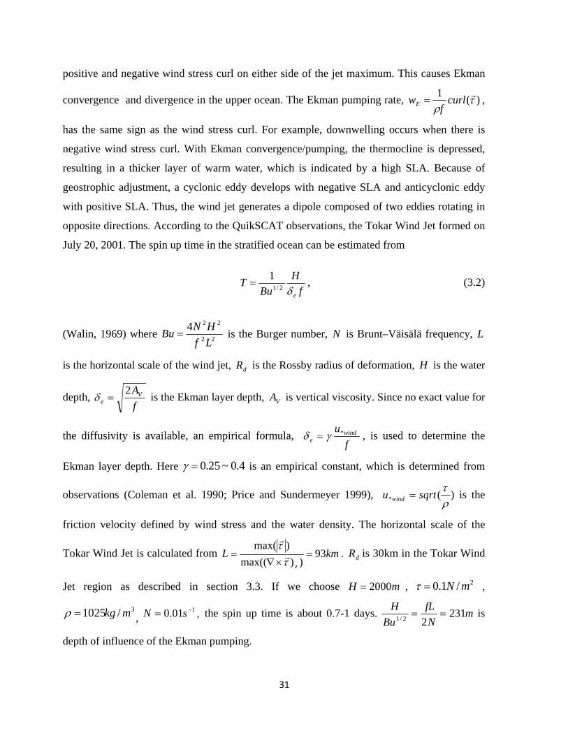
positive and negative wind stress curl on either side of the jet maximum. This causes Ekman

convergence and divergence in the upper ocean. The Ekman pumping rate, )(1

curl

fwE ,

has the same sign as the wind stress curl. For example, downwelling occurs when there is

negative wind stress curl. With Ekman convergence/pumping, the thermocline is depressed,

resulting in a thicker layer of warm water, which is indicated by a high SLA. Because of

geostrophic adjustment, a cyclonic eddy develops with negative SLA and anticyclonic eddy

with positive SLA. Thus, the wind jet generates a dipole composed of two eddies rotating in

opposite directions. According to the QuikSCAT observations, the Tokar Wind Jet formed on

July 20, 2001. The spin up time in the stratified ocean can be estimated from

f

H

BuT

e2/1

1 ,

(3.2)

(Walin, 1969) where 22

224

Lf

HNBu is the Burger number, N  is Brunt–Väisälä frequency, L  

is the horizontal scale of the wind jet, dR  is the Rossby radius of deformation, H is the water

depth, f

AVe

2 is the Ekman layer depth, VA is vertical viscosity. Since no exact value for

the diffusivity is available, an empirical formula, f

u winde

* , is used to determine the

Ekman layer depth. Here 4.0~25.0 is an empirical constant, which is determined from

observations (Coleman et al. 1990; Price and Sundermeyer 1999),

)(*

sqrtu wind is the

friction velocity defined by wind stress and the water density. The horizontal scale of the

Tokar Wind Jet is calculated from kmLz

93))max((

)max(

. dR is 30km in the Tokar Wind

Jet region as described in section 3.3. If we choose mH 2000 , 2/1.0 mN ,

3/1025 mkg , 101.0 sN ,  the spin up time is about 0.7-1 days. m

N

fL

Bu

H231

22/1 is

depth of influence of the Ekman pumping.  

32  

Figure 3.6: Sequence of the SLA (cm) during July 25, 2001 to August 29, 2001.

33  

Figure 3.7: Sequence of the QuikSCAT wind stress and the wind stress curl (unit: 10-7N/m3)

from July 25, 2001 to August 29, 2001.

34  

Figure 3.8: The August anomalies of relative vorticity at the center of the cyclonic eddy of the

dipole (black line with open circle, 106s-1) and the Tokar Wind Jet speed (red line with dot,

m/s) from 2000 to 2009. The mean values averaged from 2000 to 2009 are subtracted to get

the anomalies.

35  

Figure 3.9: Satellite ground tracks passing by the Red Sea during ±3 days of the dates shown

in the figure. en-Envisat, g2-GFO, tp-TOPEX/Poseidon, j1-Jason1.

36  

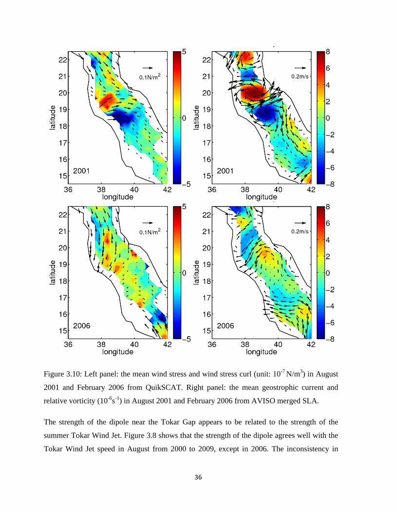
Figure 3.10: Left panel: the mean wind stress and wind stress curl (unit: 10-7 N/m3) in August

2001 and February 2006 from QuikSCAT. Right panel: the mean geostrophic current and

relative vorticity (10-6s-1) in August 2001 and February 2006 from AVISO merged SLA.

The strength of the dipole near the Tokar Gap appears to be related to the strength of the

summer Tokar Wind Jet. Figure 3.8 shows that the strength of the dipole agrees well with the

Tokar Wind Jet speed in August from 2000 to 2009, except in 2006. The inconsistency in

37  

2006 might be because of the satellite sampling issue. Figure 3.9 shows the ground tracks that

passed by the Red Sea in August 2003 and 2006. It shows that in August 2006, there are less

satellite tracks passing by the Red Sea than in August 2003. Therefore, the satellite data may

not contain enough information to resolve the strength of the dipole in 2006.

In winter, the wind converges into the Tokar gap. But the dipole generated by the winter

“convergent wind” is not as strong as in summer. Figure 3.10 shows for example, that the

westward wind jet blew continuously in February 2006. However, the response of the Red Sea

is not as obvious as in the summer. This is because the positive and negative wind stress curl

is not as strong as in summer. For example, in August 2001, the wind stress curl is larger than

5*10-7 N/m3; but in February 2006, the wind stress curl is less than 3*10-7 N/m3. In addition,

the negative wind stress curl is not comparable to the positive one in February 2006.

Therefore, more than just the magnitude of the wind stress, the structure of the wind stress

curl also plays an important role in the dipole formation.

3.3 The horizontal and vertical structure of the dipole

Up to this point, we have focused on surface expressions of the dipole near the Tokar Gap.

There is in situ observational evidence that the eddies extend below the sea surface. As

discussed above, Sofianos and Johns (2007) conducted an along-axis hydrographic and ADCP

section in August 2001, which coincided with a strong dipole event. The ADCP observations

revealed that the dipole near the Tokar Gap extended to 130 m depth.

Figure 3.11 shows three eastward velocity profiles on August 13, 2001 measured by using

shipboard ADCP. Figure 3.12 shows the locations of the profiles. The two profiles with

negative surface velocity are on two sides of the dipole. The profile with positive surface

velocity is in the middle of the dipole, the boundary between the anticyclonic and cyclonic

eddies. The velocity profiles suggest that the strength of the dipole decreases rapidly with

depth. These velocity profiles reveal a baroclinic structure of the dipole which is confined in

the upper 130 m. Figure 3.13 shows the temperature and salinity profiles of six CTD stations

which were obtained on August 12-14, 2001. The temperature profiles indicate that the

thermocline depth is about 70m on average with the maximum value at station-48. Both the

isotherms and isohalines under the anticyclonic eddy were depressed. In Figure 3.13, the

38  

thermocline depth at station 48, which is close to the center of the anticyclonic eddy, is 40 m

lower than that at station 47. According to Figure 3.13, the density difference between the

upper and the lower ocean is about 3kg/m3. Taking 1025kg/m3 as the average density, then the

surface rise at the center of the anticyclonic eddy is predicted to be cm121025

3*40 , which

is in accordance with the satellite observation (Figure 3.12). In Figure 3.12, the SLA

difference between station 47 and 48 is about 10 cm in gridded SLA on August 8, 2001. The

SLA difference between station 46 and 47 is about 4cm, which indicates that the thermocline

depth difference should be 13 m. However, the thermocline at station 46 is not uplifted as

expected. The depressed thermocline and the raised sea surface at the center of the

anticyclonic eddy, together with the horizontal velocity profiles suggest that the dipole here is

mostly the first baroclinic mode.

39  

Figure 3.11: ADCP eastward velocity profiles near the center and edges of the dipole. The

location of the velocity profiles are shown in Figure 3.12. The solid line represents the

velocity profile in the middle of the dipole which consists of two eddies rotating in opposite

directions. The dashed line represents the velocity profile on the south side of the anticyclonic

eddy and the dotted line is on the north side of the cyclonic eddy.

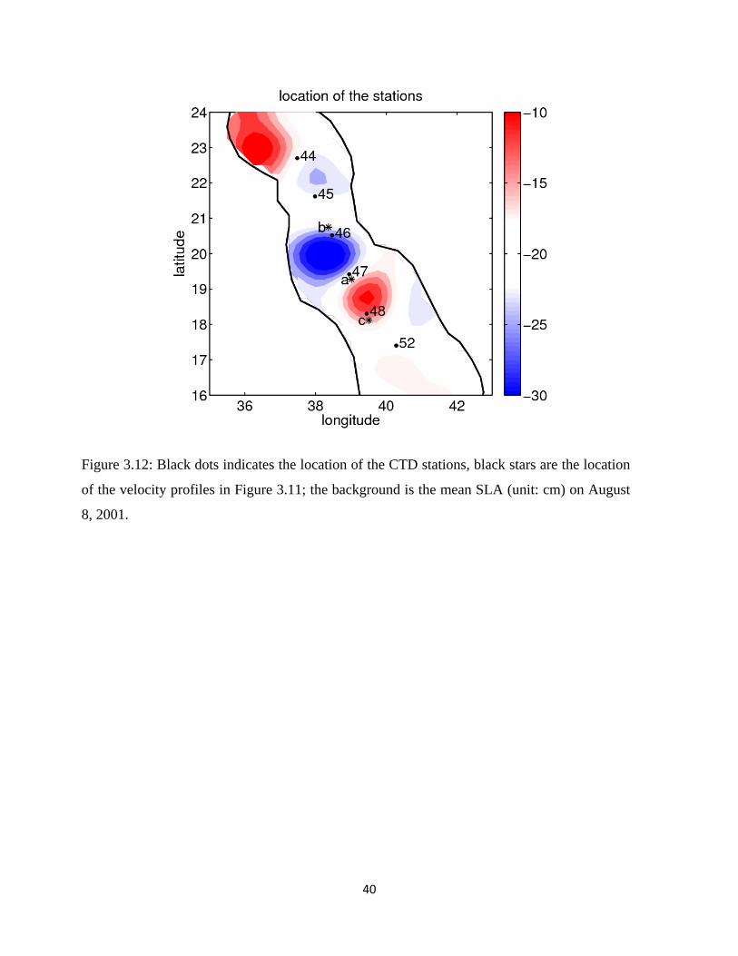
40  

Figure 3.12: Black dots indicates the location of the CTD stations, black stars are the location

of the velocity profiles in Figure 3.11; the background is the mean SLA (unit: cm) on August

8, 2001.

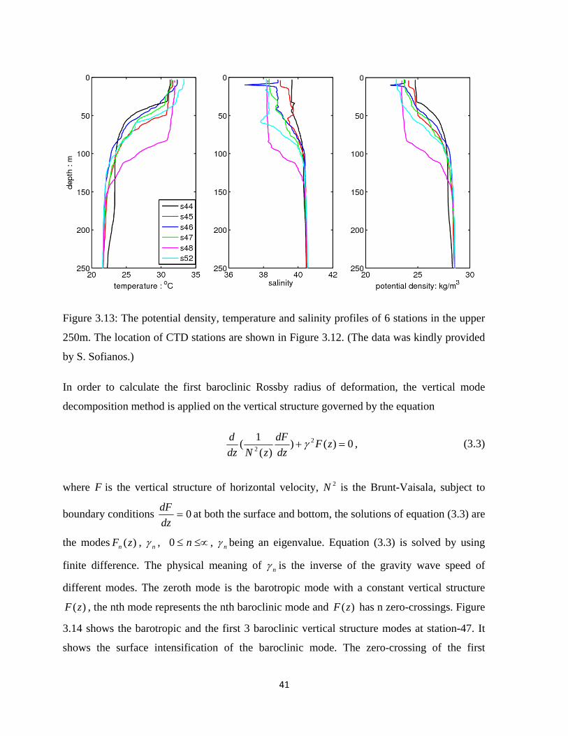
41  

Figure 3.13: The potential density, temperature and salinity profiles of 6 stations in the upper

250m. The location of CTD stations are shown in Figure 3.12. (The data was kindly provided

by S. Sofianos.)

In order to calculate the first baroclinic Rossby radius of deformation, the vertical mode

decomposition method is applied on the vertical structure governed by the equation

0)())(

1( 2

2 zF

dz

dF

zNdz

d , (3.3)

where F is the vertical structure of horizontal velocity, 2N is the Brunt-Vaisala, subject to

boundary conditions 0dz

dFat both the surface and bottom, the solutions of equation (3.3) are

the modes )(zFn , n , n0 , n being an eigenvalue. Equation (3.3) is solved by using

finite difference. The physical meaning of n is the inverse of the gravity wave speed of

different modes. The zeroth mode is the barotropic mode with a constant vertical structure

)(zF , the nth mode represents the nth baroclinic mode and )(zF has n zero-crossings. Figure

3.14 shows the barotropic and the first 3 baroclinic vertical structure modes at station-47. It

shows the surface intensification of the baroclinic mode. The zero-crossing of the first

42  

baroclinic mode is at 200m, which corresponds to the station-47’s thermocline depth of about

150 m.

The first baroclinic Rossby radius of deformation can be calculated from 1

1

1

fRd . The

values of the radius at the 6 stations are shown in Table 3.1. It indicates that the first

baroclinic Rossby radius of deformation near the anticyclonic eddy is larger than that near the

cyclonic eddy. The deformation radius calculated from the mean temperature and salinity

profiles of station 46, 47 and 48 is 30km. The eddies of the dipole are about 70km in radius

which is twice that of the first baroclinic Rossby radius of deformation.

Earlier in this chapter, it was argued that the Tokar Wind jet is responsible for the generation

of the eddy dipole. An alternative generation mechanism is baroclinic instability of the mean

flow. It seems that there is no strong mean flow in this region to generate the eddies because

the strongest flow is involved in the eddies. The dipole forms after the summer wind jet events,

when the wind near the Tokar Gap reverses its direction in winter, the dipole also reverses its

sign (Figure 3.10). While baroclinic instability could not be ruled out directly, the strength of

the dipole and that of the summer Tokar Wind Jet correlates well enough with each other that

it seems the dipole is more likely generated by the summer Tokar Wind Jet.

Table 3.1: The first baroclinic mode Rossby radius of deformation ( dR ) of 6 CTD stations.

The mean Rossby radius of deformation is calculated from the mean stratification of station

46, 47 and 48.

Station 44 45 46 47 48 52 mean

dR (km) 22 27 26 32 39 38 30

43  

Figure 3.14: Vertical structure of horizontal velocity for modes 0 to 3 at station 47.

44  

Chapter 4: Idealized simulation using a 1.5-layer model

In chapter 3, it is stated that the vertical structure of the dipole is well represented by the first baroclinic mode. The vertical mode decomposition of the horizontal velocity shows that the velocity in the lower layer is about 6% of the velocity in the upper layer for the first baroclinic mode, which indicates that the movement in the lower layer is negligible compared with the upper layer. Therefore, a 1.5-layer model is appropriate in this study to investigate the dynamics of the dipole driven by the wind jet.

4.1 The model description

In the 1.5-layer model, is also called the reduced gravity model, a single active layer with

density of 1 overlays a motionless layer of infinite thickness with different density 2 . The

momentum and continuity equations for the 1.5-layer model are

(4.1.c) 0

(4.1.b) '

(4.1.a) '

2

2

yxt

y

yyxt

x

xyxt

hvhuh

vAh

hgfuvvuvv

uAh

hgfvvuuuu

where h is the layer thickness, vu, are the horizontal velocity, sin2f is the Coriolis

parameter and changes with latitude , 1

12'

gg is the reduced gravity, yx , are the

wind stress, A is the coefficient of the lateral viscosicy. The model used here is the same as

Yang and Price (2006), except that wind forcing is added with no diapycnal mass flux. The

numerical code of 1.5-layer model is kindly provided by Jiayan yang. In this model, the

pressure gradient in the second layer vanishes and the sea level is related to the layer

thickness h by

)(1

12 Hh

(4.2)

where H is the initial thickness of the upper layer. In the 1.5-layer model, baroclinic

instability cannot occur.

45  

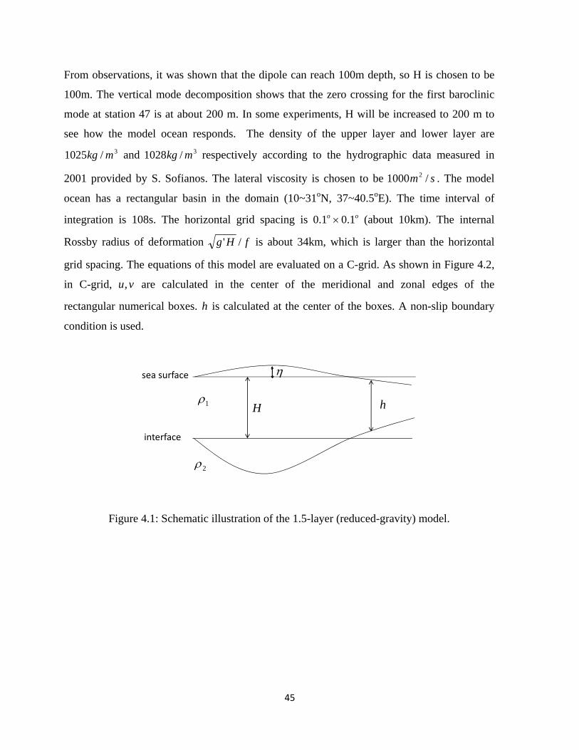
From observations, it was shown that the dipole can reach 100m depth, so H is chosen to be

100m. The vertical mode decomposition shows that the zero crossing for the first baroclinic

mode at station 47 is at about 200 m. In some experiments, H will be increased to 200 m to

see how the model ocean responds. The density of the upper layer and lower layer are

3/1025 mkg and 3/1028 mkg respectively according to the hydrographic data measured in

2001 provided by S. Sofianos. The lateral viscosity is chosen to be sm /1000 2 . The model

ocean has a rectangular basin in the domain (10~31oN, 37~40.5oE). The time interval of

integration is 108s. The horizontal grid spacing is oo 1.01.0 (about 10km). The internal

Rossby radius of deformation fHg /' is about 34km, which is larger than the horizontal

grid spacing. The equations of this model are evaluated on a C-grid. As shown in Figure 4.2,

in C-grid, vu, are calculated in the center of the meridional and zonal edges of the

rectangular numerical boxes. h is calculated at the center of the boxes. A non-slip boundary

condition is used.

Figure 4.1: Schematic illustration of the 1.5-layer (reduced-gravity) model.

hH1

2

sea surface

interface

46  

Figure 4.2: Numerical stencil of the C-grid.

4.2 The idealized simulation

The model is forced by wind fields similar to the wind jet near Tokar Gap in the summer. The

wind jet is directed offshore as shown in Equation 4.3.

)100

exp(1T(t)

)7.1)075.19(exp()(

)3/)175.37(exp()(

0

)()()(1.0

2

2

t

latitudelatitudeY

longitudelongitudeX

tTlatitudeYlongitudeXy

x

(4.3)

In Equation 4.3, the term T(t) is multiplied to the steady wind in order to reduce the impact of

inertial oscillations. Figure 4.3 shows the horizontal structure of the idealized wind jet. The

lower panel of Figure 4.3 is the comparison between the idealized wind jet and the mean

Tokar Wind Jet in August 2001. It shows that the idealized wind jet has the same magnitude

of 0.1N/m2 and spatial scale of 300 km as the mean Tokar Wind Jet in August 2001.

h

u

v

dx dy

47  

Figure 4.3: Upper panel: the idealized wind jet and the wind stress curl (10-7 N/m3) used in

the 1.5-layer model. Lower panel: the offshore direction component of the wind stress along

the middle axis of the basin. For the QuikSCAT wind, the offshore direction is 55o clockwise

relative to the north; for the wind jet in the idealized model, the offshore direction is eastward.

Figure 4.4 shows the response of the 1.5-layer model to the steady wind jet. In this experiment

(EXP1), nonlinear advection, effect and lateral friction are included. When the wind jet is

applied, the sea level drops (Figure 4.4, hour 8) at the western coast of the basin due to the

48  

offshore ageostrophic flow which is generated from the exponentially increasing wind in the

first few days. The ageostrophic current is related to the time evolution of the wind, which

was described by McCreary et al. (1989). Because of the Ekman pumping, the sea level drops

on the north of the wind jet axis and rises on the south. The meridional Ekman drift transports

water from the north to the south (Figure 4.4, hour 32). Due to the geostrophic adjustment, a

dipole including two eddies rotating in different directions spins up around the sea level

dropping center and rising center (Figure 4.4, day 8 and 30). As time goes by, the dipole

becomes stronger and moves eastward at a speed of approximately 2.1cm/s. The mechanism

of dipole’s eastward movement is shown in the Appendix.

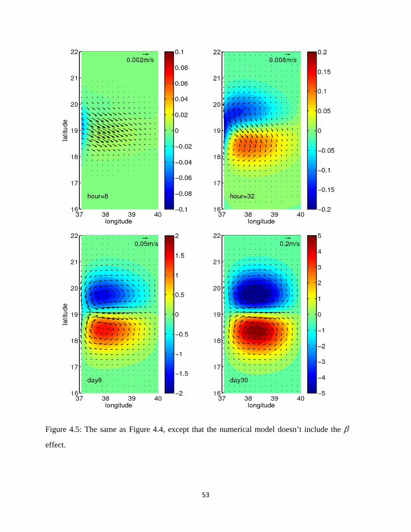
In order to investigate the impact of the effect of on the movement of the dipole, another

numerical simulation is designed—EXP2 (without effect). Figure 4.6 shows the center of

the cyclonic eddy changing with time for EXP1 and EXP2. When the Coriolis parameter f is

constant, the dipole moves eastward at a speed of 3.3cm/s, faster than in EXP1. That is

because the effect of allows for westward propagating Rossby waves which slows the self-

propagating speed of the dipole. The Rossby wave speed

222

dLlkc

, (4.4)

is 1.1cm/s if we choose the wavelength as 280km which is four times the eddy’s radius.

kmff

HgRd 34

100*1025/8.9*3' is the internal Rossby deformation radius. The

difference of the propagation speed between EXP1 and EXP2 is 1.2 cm/s, very close to the

Rossby wave speed. In EXP3 and EXP4, the density difference and H are 20 kg/m3 and 200

m respectively, and the Rossby radius of deformation is increased to 124 km. The difference

between EXP3 and EXP4 is that f changes with latitude in EXP3 while it is constant in

EXP4. The Rossby wave speed in these two experiments is 2.0 cm/s. The model results show

that in EXP4 the dipole propagates eastward 1.8 cm faster than in EXP3. The comparisons

between EXP1 and EXP2, EXP3 and EXP4 suggest that the effect of is to slow the

eastward propagation of the dipole.

49  

In chapter 3, it’s mentioned that in continuously stratified ocean, the influence depth of the

Ekman pumping is related to the buoyancy frequency and the horizontal scale of the wind. In

order to understand what influences the displacement of the interface in 1.5-layer model, the

expression of h is derived when nonlinearity is neglected. Linearized equations of motion

equations (4.1) without lateral friction are

(4.5.c) 0)(

(4.5.b) '

(4.5.a) '

yxt

yt

x

xt

vuHh

hgfuv

Hhgfvu

The equation for h is

x

yttyyxxttt

fhfhhHgh 2)('

(4.6)

If we assume that the temporal change rate of h is much slower than f , then ttth can be

neglected. For simplicity, wind stress is chosen to be )/2cos( 10 Lyx , which is different

from the wind stress used in the 1.5-layer model. If h is taken to be )/2sin()( 1LytAh ,

equation (4.6) gives

)41(

/2

)'

4(

/2

21

22

10

21

22

10

L

R

fL

L

Hgf

Lf

dt

dA

d

(4.7)

Where 22 /' fHgRd . Equation (4.7) shows that the time derivative of upper layer thickness

is related to the rotation f , the wind strength 0 , the stress jet spatial scale 1L , the reduced

gravity 'g and the initial thickness H . Since the wind is steady here, h is linearly related to

50  

dt

dA. Friction is not included in equation (4.7), therefore, h anomalies continue to grow.

Possibly friction will stop the spin up.

Table 4.1 shows results of some experiments with different parameters. The Rossby radius of

deformation varies when the density difference  or the initial thickness of the upper layer

changes. It is indicated that H and dR vary in opposite directions. That is because when

is increased, the stronger stratification makes it harder to displace the thermocline. When H

is increased, equation (4.5a) indicates that the wind effect is weakened, which lessens the

displacement of interface. The comparisons of EXP6 and EXP7, EXP9 and EXP10, EXP11

and EXP12 indicate that the density difference and the initial upper layer thickness contribute

equally to the displacement of the upper layer, which is shown in equation (4.7). There are

two effects when Coriolis parameter increases, one is that dR gets smaller and H increases,

the other one is that the Ekman pumping rate )(1

curl

fwE decreases which slows the

changing rate of h . The two effects counteract each other. Equation (4.7) shows that the

changing rate of h has an maximum value when 1

'2

L

Hgfc . If we take

2/0287.08.9*1025

3' smg , mH 100 , kmL 2001 , then when latitude is greater than

5.21c , dt

dA decreases with latitude and the Ekman pumping plays a dominant role on the

growth of h . Otherwise, when latitude is smaller than 5.21c , the growth of h depends

more on the value of Rossby radius of deformation.

The model results indicate that the dipole moves eastward because of self-advection. However,

it is hard to see in the observation from satellite SLA due to the spatial and temporal

resolution of SLA. The dipole dynamics in a 1.5-layer model is shown in the Appendix.

The experiments studied here are forced by a wind jet that is similar to the Tokar Wind Jet in

summer. When the model is forced by the wind with opposite direction which is similar to the

winter wind near the Tokar Gap, the eddies change their rotating directions. The dipole

51  

propagates westward in this case. In Figure 2.8, the Tokar Wind Jet in summer has strong

daily cycle. When the model is forced by diurnal wind jet, the variations of velocity and sea

surface also have a daily cycle. The zonal velocity has a negative component when the wind is

getting weaker as pointed out by McCreary et al. (1989, his equation 17).

For simplicity, the model ocean has a rectangular basin which is different from the Red Sea. If

a tilted basin is used in this model and the wind jet is still perpendicular to the coast, the self-

propagation speed of the dipole is not parallel to the Rossby wave propagation. Then the

dipole would move northward along the basin.

Table 4.1: Parameters and results for different numerical experiments. is density difference between the upper layer and lower layer, H is the initial thickness of the upper layer, dR is the Rossby radius of deformation, H is the magnitude of the uplifting and

depression of the upper layer at day 30.

Run Number (kg/m3) H (m) dR (km) H (m)

EXP5 0.5 50 9.8 42

EXP6 0.5 100 13.9 36

EXP7 1 50 13.9 36.7

EXP8 1 100 19.7 29.6

EXP9 3 50 24.1 25.7

EXP10 1.5 100 24.1 25.6

EXP2 3 100 34 19.5

EXP11 3 150 41.7 15.2

EXP12 1.5 300 41.7 15.2

EXP13 6 100 48.1 12.8

EXP14 10 100 62.2 9.2

EXP15 20 200 124.3 3.1

52  

Figure 4.4: The time evolution of the sea level (unit: cm) and current in the numerical model

which includes nonlinear advection, effect and lateral friction (EXP1).

53  

Figure 4.5: The same as Figure 4.4, except that the numerical model doesn’t include the

effect.

54  

Figure 4.6: The center of the cyclonic eddy changing with time in EXP1 and EXP2.

55  

Chapter 5: Conclusions and discussion

The goal of this study was to analyze the variability of the Tokar Wind Jet at different scales,

seasonal, interannual and diurnal variability, and to investigate the response of the Red Sea to

the Tokar Wind Jet. QuikSCAT wind data from 1999 to 2009 reveals that in the summer,

usually starting in July, the wind blows eastward through the Tokar Gap onto the Red Sea

surface down the pressure gradient. The summer Tokar Wind Jet can last from several days to

a month. The speed of the wind jet can reach 18m/s based on QuikSCAT records on July 12,

2008, although shipboard observations in 2001 indicate speeds as high as 20-25 m/s (S.

Sofianos, personal communication). The seasonal variability of the Tokar Wind Jet is highly

correlated with the Indian Monsoon and the pressure difference along the Tokar Gap.

Analysis of SLA indicates that after the summer Tokar Wind Jet events, a dipolar eddy,

composed of a cyclone on the north of the wind jet axis, and an anticyclone on the south,

forms in the summer. The strength of the dipole is highly influenced by the strength of the

summer Tokar Wind Jet. The geostrophic current calculated from along track SLA shows that

the surface current is as large as 1m/s. The in situ observations from Sofianos and Johns (2007)

confirmed that the maximum surface velocity of the dipole is about 1m/s. The dipolar

circulation is restricted to the upper 130 m according to ADCP velocity, salinity and

temperature profiles. Below 130 m, the flow is much weaker with the velocity smaller than

0.1m/s. The first baroclinic Rossby radius of deformation is about 30 km in the dipole region,

which is smaller than the eddies’ radius-70 km.

A 1.5-layer model was used to resolve the dipole generated by the Tokar Gap wind jet in the

summer. In response to wind forcing meant to mimic the Tokar jet, the model develops an

eddy dipole similar to ones seen in altimetric SLA. After the dipole is generated, it moves

eastward due to the self-propagation. Two numerical experiments were designed to determine

the influence of the effect. The results reveal that the effect of decreases the eastward

self-propagation speed of the dipole by the Rossby wave speed.

The analysis of the observations and numerical model results provide strong evidence that the

wind jet is the main mechanism for the generation of the dipole in summer near the Tokar Gap.

56  

McCreary et al. (1989) used a 1.5-layer model to study the dipole generated by wind jets in

Central America. The models in their work included a linear model and a nonlinear model

with entrainment. Since there is no western boundary in their model, the dipole generated by

the wind jet could propagate westward at the linear Rossby wave speed. But when there is

nonlinearity, the propagation speed of the dipole is enhanced. In our model, there is the

western boundary which makes it hard to determine the effect of . Even when there is no

advection term, the dipole cannot propagate westward because of the boundary’s barrier.

In winter, the wind blows westward into the Tokar Gap. The SLA also demonstrates the

formation of a dipole with opposite sign to the summer dipole. But the winter dipole is weaker

than the summer one. Although the magnitude of wind in summer and winter near the Tokar

Gap is similar, the wind stress curl in winter is weaker than in summer.

Since the 1.5-layer model doesn’t allow baroclinic instability, it is hard to exclude the

possibility of baroclinic instability that might be responsible for the generation of the dipole.

The 1.5-layer model forced with an idealized wind jet was able to simulate the main structure

of the dipole, which indicates that the wind jet is the main mechanism of the dipole. But a

deeper study with a 2-layer model or more complex model is needed to further explore the

dipole. Large-scale hydrographic and current surveys in the Red Sea will be conducted in the

next 2 years, with the help of the in situ data, the structure of the dipole will be studied in

detail.

57  

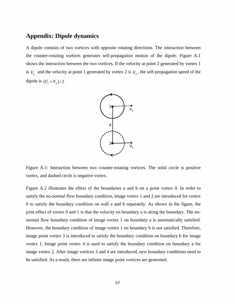
Appendix: Dipole dynamics

A dipole consists of two vortices with opposite rotating directions. The interaction between

the counter-rotating vortices generates self-propagation motion of the dipole. Figure A.1

shows the interaction between the two vortices. If the velocity at point 2 generated by vortex 1

is 2V and the velocity at point 1 generated by vortex 2 is

2V , the self-propagation speed of the

dipole is 2/)( 21 VV .

Figure A.1: Interaction between two counter-rotating vortices. The solid circle is positive

vortex, and dashed circle is negative vortex.

Figure A.2 illustrates the effect of the boundaries a and b on a point vortex 0. In order to

satisfy the no-normal flow boundary condition, image vortex 1 and 2 are introduced for vortex

0 to satisfy the boundary condition on wall a and b separately. As shown in the figure, the

joint effect of vortex 0 and 1 is that the velocity on boundary a is along the boundary. The no-

normal flow boundary condition of image vortex 1 on boundary a is automatically satisfied.

However, the boundary condition of image vortex 1 on boundary b is not satisfied. Therefore,

image point vortex 3 is introduced to satisfy the boundary condition on boundary b for image

vortex 1. Image point vortex 4 is used to satisfy the boundary condition on boundary a for

image vortex 2. After image vortices 3 and 4 are introduced, new boundary conditions need to

be satisfied. As a result, there are infinite image point vortices are generated.

1

2

d

V2

V1

58  

Figure A.2: Point vortex 0 with two boundaries a and b. Vortex 0 is the real original vortex,

vortex 1, 2, 3, 4, …… are image point vortices of vortex 0 to satisfy the no-normal flow

boundary condition. The solid circles are positive point vortex, the dashed circles are negative

point vortex; d is the distance between the vortex and wall. For example, db13 is the distance

between vortex 1 (3) and boundary b. The distance also indicates that vortex 3 is the image of

vortex 1 relative to boundary b.

In order to calculate the self-propagation speed of the dipole, the velocity structure of the

point vortex is needed. For the barotropic case, the point vortex is 2 dimensional. The solution

of

)(2 r , (A.1)

where r is the radius from the source and is the strength of the point vortex, is

rln2

, (A.2)

so that the tangential velocity

rru

2

, (A.3)

da01 da01 db02 db020 2 3

a b

4

db13 db13

1

da24 da24

…… ……

V0 V1

59  

decays from the point source as r/1 . The circulation along a circle with radius r is

dAdru 22

0.

In a 1.5-layer model, the expression for the quasi-geostrophic potential vorticity is

2

2 1

dLq . (A.4)

The solution of the 1.5-layer qgpv equation for a point vortex Qq is

)(2 0

dL

rK

Q

, (A.5)

where 0K is the zero order modified Bessel function.

Q could be calculated by integrating equation (A.4) in an area which contains the point

vortex

dAf

g

LrdudA

LQ

dd

22

2 1.)

1(

. (A.6)

In EXP1 at day 30, smQ /1081.5 24 for the anticyclonic eddy and smQ /1068.5 24

for the cyclonic eddy when integrating equation (A.6) in the area shown in Figure A.3. The

stream function for a point vortex with strength of sm /1068.5 24 ( sm /1081.5 24 for the

negative point vortex)  can be calculated from equation A.5. Then the self-propagation speed

of the dipole predicted by the point vortex in 1.5-layer model is 1.4cm/s. The self-propagation

speed predicted by the point vortex dynamics in the 1.5-layer flow is smaller than the

propagation speed 2.1cm/s in EXP1. That might be because the eddies in EXP1 are not point

vortices.

60  

Figure A.3: SSH (left panel, unit: cm) and relative vorticity (right panel, unit: 10-6s-1) at day

30 in EXP1. The cm6.0 contour of SSH defines the integral area to calculate the strength of

the vortex.

In EXP1, the flow has the eastern and western boundaries which could influence the

propagation speed of the dipole. The velocity around a point vortex decays very quickly with

radius as shown in Figure A.4. Therefore, in Figure A.2, the influence of vortex 3 and 4 on

vortex 0 could be ignored. Figure A.5 describes the influences of four image vortex while

image vortex that are not close to the real vortex are neglected.

Figure A.6 shows the trajectory of the center of the point vortex by using the velocity

structure of the point vortex in 1.5-layer. It indicates that the two eddies of the dipole move

toward each other initially while they move eastward. When they move close to the eastern

boundary, they start to move apart from each other.

61  

Figure A.4: The tangential velocity of a point vortex in the 1.5-layer model.

Figure A.5: The dipole with two boundaries. 21V represents the velocity on point vortex 1 due

to vortex 2. The solid circles are positive point vortex, the dashed circles are negative point

vortex.

13

6

5

24

V21

V51

V31

V61

V41

62  

Figure A.6: The trajectory of the center of the eddies of dipole.

63  

Reference:

Acker, J., Leptoukh, G., Shen, S., Zhu, T., Kempler, S., 2008: Remotely-sensed chlorophyll a observations of the northern Red Sea indicate seasonal variability and influence of coastal reefs. Journal of marine systems, 69, 191–204.

Cember, R. P., 1988: On the sources, formation, and circulation of Red-Sea deep-water. Journal of Geophysical Research- Oceans, 93 (C7), 8175–8191.

Cember, R. P., 1989: Bomb Radiocarbon in the Red Sea: A Medium‐Scale Gas Exchange Experiment. J. Geophys. Res., 94(C2), 2111–2123.

Clifford, M., Horton, C., Schmitz, J., Kantha, L.H., 1997: An oceanographic nowcast/forecast system for the Red Sea. Journal of Geophysical Research-Oceans, 102 (C11), 25101–25122.

Cromwell, D., and Smeed, D. A., 1998: Altimetric observations of sea level cycles near the Strait of Bab al Mandab. Int. J. Remote Sens., 19, 1561–1578.

Coleman, G. N., Ferziger, J. H. and Spalart, P. R., 1990: A numerical study of the turbulent Ekman layer. J. Fluid Mech., 213, 313-348.

Ducet, N., P. Y. Le Traon, and G. Reverdin, 2000: Global high-resolution mapping of ocean circulation from TOPEX/Poseidon and ERS-1 and -2, J. Geophys. Res., 105(C8), 19,477–19,498, doi:10.1029/2000JC900063.

Fairall, C.W., E.F. Bradley, J.E. Hare, A.A. Grachev, and J.B. Edson, 2003: Bulk parameterization of air-sea fluxes: Updates and verification for the COARE algorithm. J. Climate, 16, 571–591.

Fu, L.-L., E. J. Christensen, C. A. Yamarone Jr., M. Lefebvre, Y. Menard, M. Dorrer, and P. Escudier, 1994: TOPEX/POSEIDON mission overview, J. Geophys. Res., 99, 24,369–24,381.

Greenspan, H. P., 1968: The Theory of Rotating Fluids. Cambridge University Press, p36.

Hellerman, S., and M. Rosenstein, 1983: Normal monthly wind stress over the world ocean with error estimates. J. Phys. Ocean., 13, 1093–1104.

Hernandez, F.and P. Schaeffer, 2001: A mean sea surface dedicated to merge T/P, Jason-1, ERS-2, ENVISAT, and GFO altimetric data.

Hickey, B., and A. S. Goudie, 2007: The use of TOMS and MODIS to identify dust storm source areas: The Tokar delta (Sudan) and the Seistan basin (south west Asia), in Geomorphological Variations, edited by A. S. Goudie and J. Kalvoda, pp. 37– 57, P3K, Prague.

64  

Jet Propulsion Laboratory, 2001: SeaWinds on QuikSCAT Level 3: Daily, Gridded Ocean Wind Vectors ( JPL SeaWinds Project), Guide Document Version 1.1.

Jiang, H., J. T. Farrar, R. C. Beardsley, R. Chen, and C. Chen, 2009: Zonal surface wind jets across the Red Sea due to mountain gap forcing along both sides of the Red Sea, Geophys. Res. Lett., 36, L19605, doi: 10.1029/2009GL040008.

Large W. G., and Pond S., 1981: Open ocean momentum flux measurement in moderate to strong winds. J. Phys. Oceanogr., 11, 324–336

Maillard, C., Soliman, G., 1986: Hydrography of the Red Sea and exchanges with the Indian Ocean in summer. Oceanology Acta, 9, 249–269.

McCreary, J. P., H. S. Lee, and D. B. Enfield, 1989: Response of the coastal ocean to strong offshore winds: With application to circulations in the Gulf of Tehuantepec and Papagayo. J. Mar. Res., 47, 81–109.

Morcos, S., 1970: Physical and chemical oceanography of the Red Sea. Oceanogr. Mar. Biol., 8, 73–202.

Morcos, S., and G. F. Soliman, 1972: Circulation and deep water formation in the northern Red Sea in winter. L’Oceanographie Physique de la Mer Rouge, UNESCO, 91–103.

Murray, S.P., Johns, W., 1997: Direct observations of seasonal exchange through the Bab el Mandeb strait. Geophysical Research Letters, 24, 2557–2560.

Neumann, A.C., McGill, D.A., 1962: Circulation of the Red Sea in early summer. Deep-Sea Research, 8, 223–235.

Patzert, W.C., 1974: Volume and heat transports between the Red Sea and Gulf of Aden, notes on the Red Sea heat budget. In: L’oceanographie physique de la Mer Rouge, CNEXO, Paris, pp. 191–201.

Pedgley, D., 1972: Desert depression over north-east Africa. Met. Mag. 101, 228–243.

Pedgley, D.E., 1974. An outline of the weather and climate of the Red Sea. In: L’oceanographie physique de la Mer Rouge, CNEXO, Paris, pp. 9–27.

Pickett, M.H., Tang, W., Rosenfeld, L.K., Wash, C.H., 2003: QuikSCAT satellite comparisons with nearshore buoy wind data off the U.S. west coast. J. Atmos. Oceanic Technol., 20, 1869–1979.

Plähn, O., B. Baschek, T. H. Badewien, M. Walter, and M. Rhein, 2002: Importance of the Gulf of Aqaba for the formation of bottom water in the Red Sea. J. Geophys. Res., 107(C8), 3108, doi:10.1029/2000JC000342.

Pratt, L., Albright, E. J., Jiang, H., The Tokar Wind Jet: Observations and Analysis based on the WRF Model, unpublished paper.

65  

Price, J. F., and M. A. Sundermeyer, 1999: Stratified Ekman layers. J. Geophys. Res., 104(C9), 20,467–20,494, doi:10.1029/1999JC900164.

Quadfasel, D., Baudner, H., 1993: Gyre-scale circulation cells in the Red-Sea. Oceanologica Acta, 16 (3), 221–229.

Satheesan, K., Sarkar, A., Parekh, A., Ramesh Kumar, M.R., Kuroda, Y., 2007: Comparison of wind data from QuikSCAT and buoys in the Indian Ocean. Int. J. Remote Sensing, 10, 2375–2382.

Smeed, D.A., 2004: Exchange through the Bab el Mandab. Deep-Sea Research, II 51, 455–474.

Sofianos, S. S., and W. E. Johns, 2001: Wind induced sea level variability in the Red Sea, Geophys. Res. Lett., 28, 3175– 3178.

Sofianos, S. S., W. E. Johns, and S. P. Murray, 2002: Heat and freshwater budgets in the Red Sea from direct observations at Bab el Mandeb. Deep Sea Res., Part II, 49, 1323– 1340.

Sofianos, S. S., and W. E. Johns, 2003: An Oceanic General Circulation Model (OGCM) investigation of the Red Sea circulation: 2. Three-dimensional circulation in the Red Sea, J. Geophys. Res., 108(C3), 3066, doi:10.1029/2001JC001185.

Sofianos, S. S., and W. E. Johns, 2007: Observations of the summer Red Sea circulation, J. Geophys. Res., 112, C06025, doi:10.1029/2006JC003886.

Walin, G., 1969: Some aspects of time-dependent motion of a stratified rotating fluid. J. Fluid Mech, 36, 289–307.

Wang, B., R. Wu, K.-M. Lau, 2001: Interannual variability of Asian summer monsoon: Contrast between the Indian and western North Pacific-East Asian monsoons. J. Climate, 14, 4073–4090.

Werner, F. and K. Lange., 1975: A Bathymetric Survey of the Sill Area between the Red Sea and the Gulf of Aden. Geol. Jahrb. D, 13: 125–130.

Yang, J., J. F. Price, 2007: Potential Vorticity Constraint on the Flow between Two Basins. J. Phys. Oceanogr., 37, 2251–2266. doi: 10.1175/JPO3116.1.