CWP-546

Recursive Gaussian filters

Dave HaleCenter for Wave Phenomena, Colorado School of Mines, Golden CO 80401, USA

ABSTRACTGaussian or Gaussian derivative filtering is in several ways optimal for applica-tions requiring low-pass filters or running averages. For short filters with lengthsof a dozen samples or so, direct convolution with a finite-length approximationto a Gaussian is the best implementation. However, for longer filters such asthose used in computing running averages, recursive implementations may bemuch more efficient. Based on the filter length, we select one of two popularmethods for designing and implementing recursive Gaussian filters.

Key words: digital signal processing

1 INTRODUCTION

Gaussian filtering is useful in at least two different con-texts in digital signal processing. One context is low-passfiltering. In this context, we typically wish to attenu-ate high-frequency noise. For example, when detectingedges or computing the orientation of features in digitalimages, we might compute partial derivatives of imagesample values (van Vliet and Verbeek, 1995). Becausederivatives amplify high-frequency (often noisy) com-ponents of signals, we might also apply a low-pass filterbefore or after computing those derivatives.

An equivalent and more efficient process is to applya filter that combines both differentiation and low-passfiltering. When the low-pass filter is a Gaussian, thiscombination yields a filter with a smooth impulse re-sponse that approximates a derivative of a Gaussian.

Another context in which Gaussian filtering is use-ful is in computing running averages. We often use run-ning averages to estimate parameters from signals withcharacteristics that vary with space and time. A typicalexample looks something like this:

y(t) =1

2T

∫ t+T

t−T

ds x(s). (1)

Here, we estimate a parameter y that varies with time tby averaging nearby values of some other function x(t).Ideally, we choose the window length 2T large enoughto obtain meaningful estimates of the parameter y, butsmall enough that we can detect significant variationsin that parameter with time t.

Running averages like that in equation 1 appear

often in seismic data processing. For example, in coda-wave interferometry (Snieder, 2006) the function x(t) isthe product of two seismograms, one shifted relative tothe other. In seismic velocity estimation, the functionx(t) might be the numerator or denominator sum ina semblance calculation (Neidell and Taner, 1971). Atrivial example is automatic gain control, in which y(t)might be an rms running average of seismic amplitudecomputed as a function of recording time t.

In each of these applications, we might ask whetherthe averaging in equation 1 is sensible. For each estimatey(t), this equation implies that all values x(s) inside thewindow of length 2T have equal weight, but that valuesjust outside this window have no weight at all.

This weighting makes no sense. In estimating y(t),why should the values x(t) and x(t + T − ε) get equalweight, but the value x(t + T + ε) get zero weight? Amore sensible window would give values x(s) for s near thigher weight than values farther away. In other words,we should use a weighted average, a window with non-constant weights. And the uncertainty relation (e.g.;Bracewell, 1978) tells us that the optimal window isGaussian.

A sampled version of equation 1 is

y[n] =1

2M + 1

n+M∑m=n−M

x[m]. (2)

Despite the shortcoming described above, this sort ofrunning average may be popular because we can easilyand efficiently implement it by solving recursively thefollowing linear constant-coefficient difference equation:

2 D. Hale

y[n] = y[n−1] + (x[n+M ]− x[n−M−1])/(2M+1), (3)

with some appropriate initial and end conditions. Forlong windows (large M) we must take care to avoid ex-cessive accumulation of rounding errors as we add andsubract small sample values x[n + M ] and x[n−M − 1]from the previous output value y[n− 1]. For short win-dows (small M) we might use the non-recursive runningaverage of equation 2. But it is difficult to achieve acomputational cost lower than that of equation 3.

The two contexts described above — low-pass fil-tering and running averages — are of course one and thesame. A running average is a low-pass filter. In practice,these contexts differ only in the length of the filter re-quired. Gaussian derivative filters typically have shortlengths of less than 10 samples. Gaussian filters usedin running averages tend to be longer, sometimes withlengths of more than 100 samples.

In this paper, we compare two recursive implemen-tations of Gaussian and Gaussian derivative filters. As inequation 3, these filters solve difference equations. Nu-merical tests indicate that one implementation is bestfor short filters (derivatives), while the other is best forlong filters (running averages). For long filters, espe-cially, recursive implementations are much more efficientthan direct convolution with truncated or tapered sam-pled Gaussians.

2 THE GAUSSIAN AND DERIVATIVES

The Gaussian function is defined by

g(t; σ) ≡ 1√2πσ

e−t2/2σ2, (4)

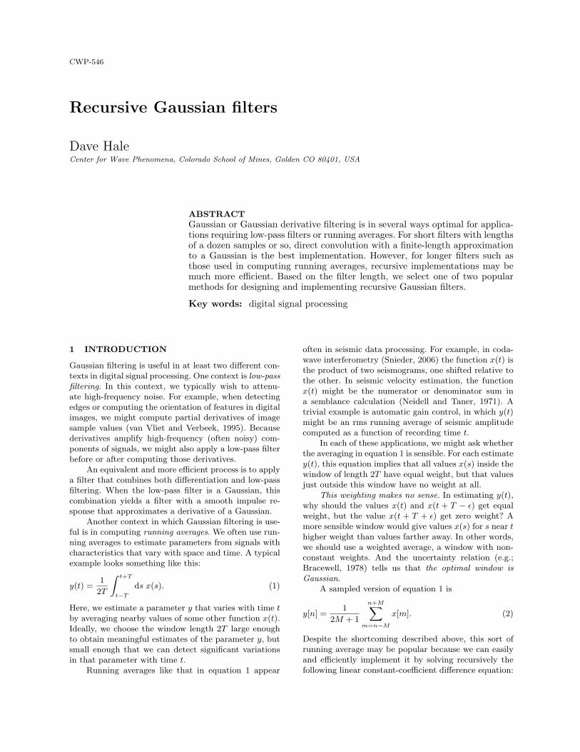
where the parameter σ denotes the Gaussian half-width.Figure 1 displays this Gaussian function and its 1st and2nd derivatives for σ = 1.

The Fourier transform of the Gaussian function isalso a Gaussian:

G(ω; σ) ≡∫ ∞

−∞dt e−iωtg(t; σ) = e−ω2σ2/2. (5)

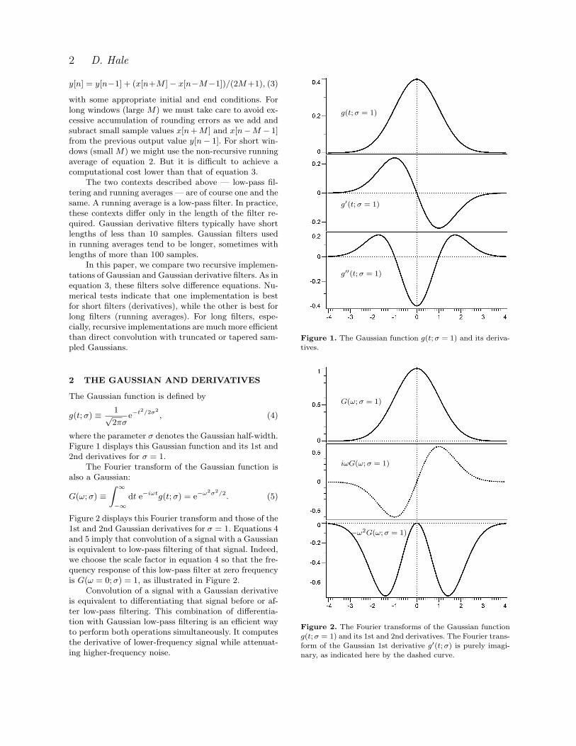
Figure 2 displays this Fourier transform and those of the1st and 2nd Gaussian derivatives for σ = 1. Equations 4and 5 imply that convolution of a signal with a Gaussianis equivalent to low-pass filtering of that signal. Indeed,we choose the scale factor in equation 4 so that the fre-quency response of this low-pass filter at zero frequencyis G(ω = 0; σ) = 1, as illustrated in Figure 2.

Convolution of a signal with a Gaussian derivativeis equivalent to differentiating that signal before or af-ter low-pass filtering. This combination of differentia-tion with Gaussian low-pass filtering is an efficient wayto perform both operations simultaneously. It computesthe derivative of lower-frequency signal while attenuat-ing higher-frequency noise.

g(t; σ = 1)

g′(t; σ = 1)

g′′(t; σ = 1)

Figure 1. The Gaussian function g(t; σ = 1) and its deriva-

tives.

G(ω; σ = 1)

iωG(ω; σ = 1)

−ω2G(ω; σ = 1)

Figure 2. The Fourier transforms of the Gaussian function

g(t; σ = 1) and its 1st and 2nd derivatives. The Fourier trans-

form of the Gaussian 1st derivative g′(t; σ) is purely imagi-nary, as indicated here by the dashed curve.

Recursive Gaussian filters 3

2.1 Sampling and aliasing

For digital filtering, we must sample the Gaussian func-tion g(t; σ) and its derivatives. Because the Fouriertransform G(ω; σ) is nowhere zero, the Gaussian func-tion cannot be sampled without aliasing. However, alias-ing can in most applications be negligible.

For definiteness, assume a unit sampling interval∆t = 1. Then, for half-width σ = 1 and the Nyquistfrequency ω = π, the Fourier transform is G(π; σ = 1) ≈0.0072. (See Figure 2.) This small magnitude impliesthat the Gaussian function g(t; σ ≥ 1) can be sampledwith unit sampling interval without significant aliasing.

The impact of aliasing is application dependent,but we typically do not sample Gaussians for whichσ < 1. For applications requiring almost no aliasing,we might choose σ ≥ 2, because G(π; σ ≥ 2) < 10−8.

As illustrated in Figure 2, the Fourier transformsof the derivatives g′(t; σ) and especially g′′(t; σ) do notapproach zero so quickly. In some applications, Gaussianderivatives may require a larger half-width σ > 1 toavoid significant aliasing.

2.2 FIR approximations

Just as we may reasonably assume that the Fouriertransform G(ω; σ) has finite bandwidth, so may we as-sume that the Gaussian function itself has finite sup-port. Figure 1 suggests that the Gaussian function andits derivatives are approximately zero for |t| > 4σ. Forexample, g(t; σ) < 0.0004 for |t| > 4σ.

Again, assume a unit sampling interval, and let h[n]denote a sampled Gaussian function that has been trun-cated or tapered to zero for |n| > M ≈ 4σ. Gaussianfiltering can then be performed via direct convolution:

y[n] =

n+M∑m=n−M

h[n−m]x[m].

This convolution is reminiscent of equation 2.Exploiting symmetry in the filter h[m], this finite-

impulse-response (FIR) approximation to Gaussian fil-tering requires roughly 1 + 4σ multiplications and 8σadditions per output sample. The computational costof applying an FIR Gaussian or Gaussian derivative fil-ter grows linearly with the Gaussian half-width σ.

2.3 IIR approximations

In constrast, the cost of an infinite-impulse-response(IIR) approximation to Gaussian filtering is indepen-dent of the half-width σ. IIR Gaussian and Gaussianderivative filters solve recursively a sequence of differ-ence equations like this one:

y[n] = b0x[n] + b1x[n− 1] + b2x[n− 2]

− a1y[n− 1]− a2y[n− 2], (6)

where the filter coefficients b0, b1, b2, a1, and a2 are somefunction of the Gaussian half-width σ. This differenceequation is reminiscent of equation 3.

The recursive solution of a single difference equa-tion cannot well approximate Gaussian filtering. Withonly five parameters, we cannot shape the impulse re-sponse of this system to fit well the Gaussian function.Moreover, the impulse response of the system of equa-tion 6 is one-sided, not symmetric like the Gaussianfunction in Figure 1. IIR symmetric filtering requiresa sequence of solutions to both causal and anti-causalsystems.

The z-transform of the IIR filter implied by equa-tion 6 is

H+(z) =b0 + b1z

−1 + b2z−2

1 + a1z−1 + a2z−2.

Assuming that all poles of H+(z) lies inside the unitcircle in the complex z-plane, this 2nd-order system isboth causal and stable. A corresponding stable and anti-causal 2nd-order system is

H−(z) =b0 + b1z + b2z

2

1 + a1z + a2z2,

for which all poles lie outside the unit circle.Neither of these 2nd-order recursive systems is suf-

ficient for Gaussian filtering. But by combining causaland anti-causal systems like these, we can constructhigher-order recursive systems with symmetric impulseresponses that closely approximate the Gaussian func-tion.

3 TWO METHODS

Deriche (1992) and van Vliet et al. (1998) describe dif-ferent methods for designing recursive Gaussian andGaussian derivative filters. Both methods are widelyused in applications for computer vision.

In their designs, both methods exploit the scalingproperties of Gaussian functions and their Fourier trans-forms. Specifically, from equations 4 and 5, we have

g(t; σ) =σ0

σg(tσ0/σ; σ0)

and

G(ω; σ) = G(ωσ/σ0; σ0).

This scaling property implies that poles and zeros com-puted for a Gaussian filter with half-width σ0 can beused to quickly construct Gaussian filters for any half-width σ.

To understand this construction, consider one fac-tor for one pole of a Gaussian filter designed for half-width σ0:

H(z; σ0) =1

1− eiω0z−1× H̃(z; σ0),

4 D. Hale

where H̃(z; σ0) represents all of the other factors cor-responding to the other poles and zeros of this system.The factor highlighted here has a single complex pole at

z = eiω0 = ei(ν0+iµ0) = e−µ0eiν0 .

For this factor to represent a causal stable system, thispole must lie inside the unit circle in the complex z-plane, so we require µ0 > 0. In other words, stability ofthe causal factor requires that the pole lies in the upperhalf of the complex ω-plane.

Substituting z = eiω, the frequency response of thissystem is

H(ω; σ0) =1

1− ei(ω0−ω)× H̃(ω; σ0).

Now use the scaling property to design a new systemwith half-width σ:

H(ω; σ) ≈ H(ωσ; σ0) =1

1− ei(ω0−ωσ)× H̃(ωσ; σ0).

The scaling property here holds only approximately, be-cause the frequency response H(ω; σ) only approximatesthe frequency response G(ω; σ) of an exact Gaussian fil-ter.

The pole of the new system is at ω = ω0/σ in thecomplex ω-plane or at

z = eiω0/σ = e−µ0/σeiν0/σ

in the complex z-plane. A similar scaling applies to allpoles of the new system.

Note that increasing σ causes the poles of the sys-tem H(z; σ) to move closer to the unit circle, yielding alonger impulse response, consistent with a wider Gaus-sian.

3.1 Deriche

Deriche (1992) constructs recursive Gaussian filters asa sum of causal and anti-causal systems:

H(z) = H+(z) + H−(z).

For Deriche’s 4th-order filters, the causal system is

H+(z) =b+0 + b+

1 z−1 + b+2 z−2 + b+

3 z−3

1 + a1z−1 + a2z−2 + a3z−3 + a4z−4,

and the anti-causal system is

H−(z) =b−1 z + b−2 z2 + b−3 z3 + b−4 z4

1 + a1z + a2z2 + a3z3 + a4z4.

To implement the composite system H(z), we applyboth causal and anti-causal filters to an input sequencex[n], and accumulate the results in an output sequencey[n]. We apply the causal and anti-causal filters in par-allel.

The coefficients a1, a2, a3, and a4 depend only onthe locations of the filter poles, and these coefficientsare the same for both the causal system H+(z) and theanti-causal system H−(z).

The coefficients b+1 , b+

2 , b+3 , and b+

4 in the causalsystem H+(z) depend on the locations of the filter zeros.

The coefficients b−1 , b−2 , b−3 , and b−4 in H−(z) areeasily computed from the other coefficients, because thecomposite filter H(z) must be symmetric. That is, werequire H(z) = H+(z) + H−(z) = H(z−1). Therefore,

b−1 = b+1 − b+

0 a1

b−2 = b+2 − b+

0 a2

b−3 = b+3 − b+

0 a3

b−4 = − b+0 a4.

With these relations, the eight coefficients of thecausal system H+(z) determine completely the sym-metric impulse response h[n] of the composite systemH(z). Those eight coefficients, in turn, depend on thepoles and zeros of the causal system H+(z).

Deriche computes these poles and zeros to minimizea sum

E =

N∑n=0

[h[n]− g(n; σ0)]2

of squared differences between the impulse response h[n]and the sampled Gaussian function with half-width σ0.Deriche chooses σ0 = 100 and N = 10σ0 = 1000.

A solution to this non-linear least-squares mini-mization problem is costly, but need be computed onlyonce. After computing poles and zeros to approximatea Gaussian with half-width σ0, Deriche uses the scalingproperties to obtain poles and zeros for other σ.

Deriche solves a similar minimization problem toobtain poles and zeros for systems with impulse re-sponses that approximate Gaussian 1st and 2nd deriva-tives.

3.2 van Vliet, Young, and Verbeek

van Vliet, Young and Verbeek (1998) construct recursiveGaussian filters as a product of causal and anti-causalsystems:

H(z) = H+(z)×H−(z).

For van Vliet et al.’s 4th-order filters, the causal systemis

H+(z) =b0

1 + a1z−1 + a2z−2 + a3z−3 + a4z−4,

and the anti-causal system is

H−(z) =b0

1 + a1z + a2z2 + a3z3 + a4z4.

To implement the composite system H(z), we first applythe causal filter to an input sequence x[n] to obtain anintermediate output sequence y+[n]. We then apply theanti-causal filter to that sequence y+[n] to obtain a finaloutput sequence y[n]. In this implementation, we applythe causal and anti-causal filters in series.

Once again, the coefficients a1, a2, a3, and a4 de-pend only on the locations of the filter poles, and these

Recursive Gaussian filters 5

coefficients are the same for both the causal systemH+(z) and the anti-causal system H−(z). The sym-metry of this system is easily verified; that is, H(z) =H+(z)×H−(z) = H(z−1).

van Vliet et al. compute the filter poles in two ways.They minimize either the rms error

L2 =

{1

2π

∫ π

−π

dω [H(ω; σ0)−G(ω; σ0)]2

}1/2

or the maximum error

L∞ = max|ω|<π

|H(ω; σ0)−G(ω; σ0)|

in the frequency responses H(ω; σ) of the filters. Foreither error, they compute poles for σ0 = 2, and thenscale those poles to obtain Gaussian filters for other σ.

For Gaussian filters, van Vliet et al. show that therms and maximum errors do not differ significantly forpoles computed by minimizing either error.

For Gaussian derivative filters, van Vliet et al.propose the application of centered finite-difference fil-ters before or after Gaussian filtering. The 1st-finite-difference system is

D1(z) =1

2(z − z−1),

and the 2nd-finite-difference system is

D2(z) = z − 2 + z−1.

These finite-difference filters only approximate differen-tiation, and the approximation is best for low frequen-cies where

D1(ω) = i sin ω ≈ iω

and

D2(ω) = −2(1− cos ω) ≈ −ω2.

For higher frequencies, the error in these approxima-tions may be significant.

3.3 Serial or parallel implementation

An advantage highlighted by van Vliet et al. is that theirsystem has only poles, no zeros, and therefore requiresfewer multiplications and additions than does Deriche’sparallel system. A serial cascade of causal and anti-causal all-pole IIR filters is less costly than a compa-rable parallel (or serial) system of IIR filters with bothpoles and zeros.

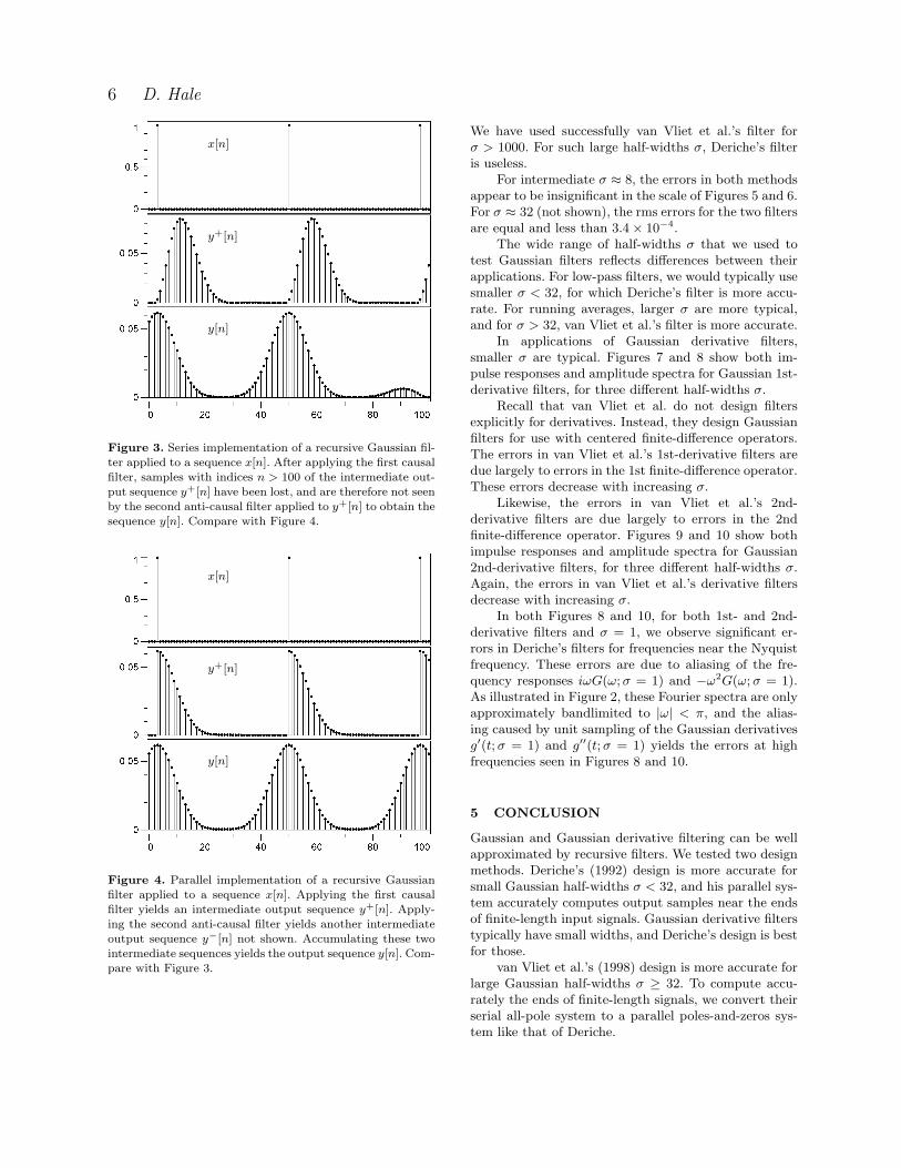
Unfortunately, a disadvantage of any system thatcascades causal and anti-causal filters lies in filteringsequences that have finite-length. To see this, assume aninput sequence x[n] with length N samples. Specifically,the input sequence x[n] is non-zero for only 0 ≤ n < N .Typically, we want a filtered output sequence y[n] withthe same length.

To compute the filtered output sequence y[n], we

first apply the causal recursive filter of our cascadesystem to the finite-length sequence x[n] to obtain anintermediate sequence y+[n] that has infinite length.The intermediate sequence y+[n] may be non-zero for0 ≤ n < ∞. If we simply truncate that sequence y+[n]to zero for n ≥ N , we discard samples that should beinput to the second anti-causal recursive filter of ourcascade system. The output sequence y[n] is then incor-rect, with significant errors for sample indices n ≈ N .Figure 3 illustrates these errors with a simple example.

We might instead compute an extended intermedi-ate sequence y+[n] for sample indices 0 ≤ n < N + L,where L is the effective length of the first causal IIR fil-ter. Beyond some length L, the impulse response of thatfilter may be approximately zero, and so may be negli-gible. For Gaussian filters with large half-widths σ, thiseffective length may be significant and costly in bothmemory and computation.

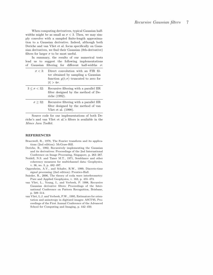
An alternative to estimating and using an effectivelength is to simply convert van Vliet et al.’s cascade sys-tem into an equivalent parallel system, using the methodof partial fractions (e.g., Oppenheim and Schafer, 1999).In other words, we may use the cascade all-pole design ofvan Vliet et al. (1998) with the parallel poles-and-zerosimplementation of Deriche (1992). Figure 4 illustratesthis alternative parallel implementation.

A 4th-order parallel implementation of either De-riche’s or van Vliet et al.’s recursive Gaussian filter re-quires 16 multiplications and 14 additions per outputsample. This cost is independent of the Gaussian half-width σ.

Compare this cost with that for a non-recursive FIRfilter obtained by sampling a Gaussian function g(t; σ)that has been truncated to zero for |t| > 4σ: 1+4σ mul-tiplications and 8σ additions. Assuming that the com-putational cost of a multiplication and addition are thesame, a parallel recursive implementation is more effi-cient for σ > 2.5.

4 NUMERICAL TESTS

To test the design methods of Deriche and van Vliet etal., we used both methods to compute filter poles andzeros for 4th-order Gaussian and Gaussian derivativefilters. We implemented both filters as parallel systems.While a parallel implementation of van Vliet et al.’sfilter is no more efficient than Deriche’s, it eliminatesthe truncation errors described above.

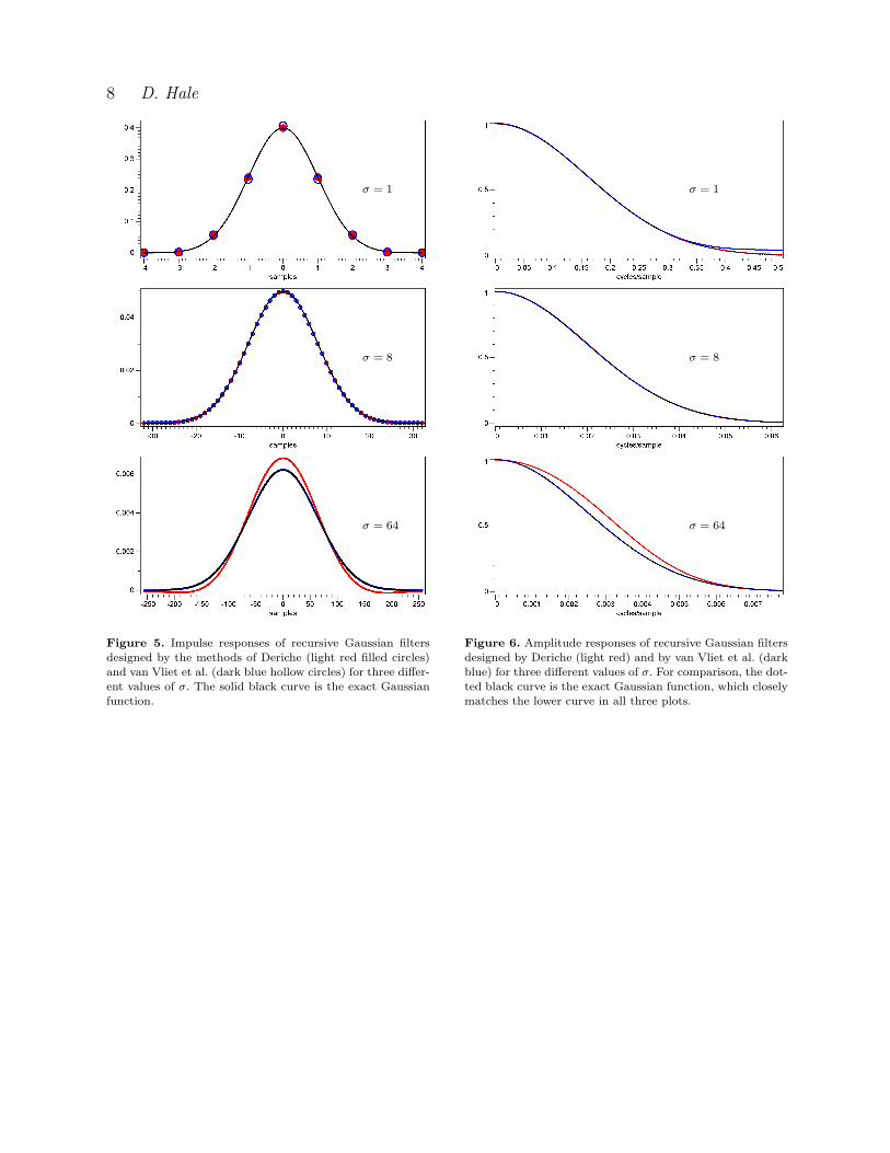
Figures 5 and 6 show both impulse responses andamplitude spectra for Gaussian (0th-derivative) filters,for three different half-widths σ. For small σ ≈ 1, De-riche’s filter is more accurate than van Vliet et al.’sfilter, and the difference is most significant for higherfrequencies.

However, for large σ ≈ 64, Deriche’s filter is muchless accurate than van Vliet et al.’s filter; the accuracyof Deriche’s filter degrades quickly with increasing σ.

6 D. Hale

x[n]

y+[n]

y[n]

Figure 3. Series implementation of a recursive Gaussian fil-

ter applied to a sequence x[n]. After applying the first causalfilter, samples with indices n > 100 of the intermediate out-

put sequence y+[n] have been lost, and are therefore not seen

by the second anti-causal filter applied to y+[n] to obtain thesequence y[n]. Compare with Figure 4.

x[n]

y+[n]

y[n]

Figure 4. Parallel implementation of a recursive Gaussianfilter applied to a sequence x[n]. Applying the first causalfilter yields an intermediate output sequence y+[n]. Apply-

ing the second anti-causal filter yields another intermediateoutput sequence y−[n] not shown. Accumulating these two

intermediate sequences yields the output sequence y[n]. Com-

pare with Figure 3.

We have used successfully van Vliet et al.’s filter forσ > 1000. For such large half-widths σ, Deriche’s filteris useless.

For intermediate σ ≈ 8, the errors in both methodsappear to be insignificant in the scale of Figures 5 and 6.For σ ≈ 32 (not shown), the rms errors for the two filtersare equal and less than 3.4× 10−4.

The wide range of half-widths σ that we used totest Gaussian filters reflects differences between theirapplications. For low-pass filters, we would typically usesmaller σ < 32, for which Deriche’s filter is more accu-rate. For running averages, larger σ are more typical,and for σ > 32, van Vliet et al.’s filter is more accurate.

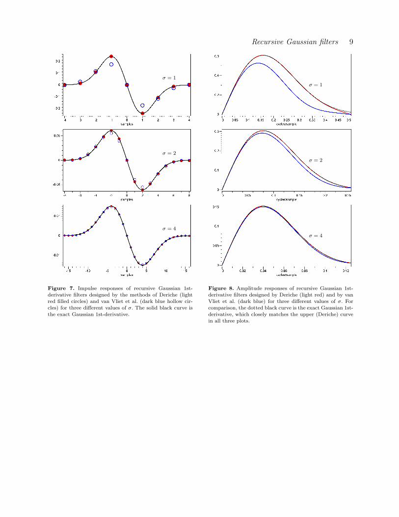
In applications of Gaussian derivative filters,smaller σ are typical. Figures 7 and 8 show both im-pulse responses and amplitude spectra for Gaussian 1st-derivative filters, for three different half-widths σ.

Recall that van Vliet et al. do not design filtersexplicitly for derivatives. Instead, they design Gaussianfilters for use with centered finite-difference operators.The errors in van Vliet et al.’s 1st-derivative filters aredue largely to errors in the 1st finite-difference operator.These errors decrease with increasing σ.

Likewise, the errors in van Vliet et al.’s 2nd-derivative filters are due largely to errors in the 2ndfinite-difference operator. Figures 9 and 10 show bothimpulse responses and amplitude spectra for Gaussian2nd-derivative filters, for three different half-widths σ.Again, the errors in van Vliet et al.’s derivative filtersdecrease with increasing σ.

In both Figures 8 and 10, for both 1st- and 2nd-derivative filters and σ = 1, we observe significant er-rors in Deriche’s filters for frequencies near the Nyquistfrequency. These errors are due to aliasing of the fre-quency responses iωG(ω; σ = 1) and −ω2G(ω; σ = 1).As illustrated in Figure 2, these Fourier spectra are onlyapproximately bandlimited to |ω| < π, and the alias-ing caused by unit sampling of the Gaussian derivativesg′(t; σ = 1) and g′′(t; σ = 1) yields the errors at highfrequencies seen in Figures 8 and 10.

5 CONCLUSION

Gaussian and Gaussian derivative filtering can be wellapproximated by recursive filters. We tested two designmethods. Deriche’s (1992) design is more accurate forsmall Gaussian half-widths σ < 32, and his parallel sys-tem accurately computes output samples near the endsof finite-length input signals. Gaussian derivative filterstypically have small widths, and Deriche’s design is bestfor those.

van Vliet et al.’s (1998) design is more accurate forlarge Gaussian half-widths σ ≥ 32. To compute accu-rately the ends of finite-length signals, we convert theirserial all-pole system to a parallel poles-and-zeros sys-tem like that of Deriche.

Recursive Gaussian filters 7

When computing derivatives, typical Gaussian half-widths might be as small as σ < 3. Then, we may sim-ply convolve with a sampled finite-length approxima-tion to a Gaussian derivative. Indeed, although bothDeriche and van Vliet et al. focus specifically on Gaus-sian derivatives, we find their Gaussian (0th-derivative)filters for larger σ to be most useful.

In summary, the results of our numerical testslead us to suggest the following implementationsof Gaussian filtering for different half-widths σ:

σ < 3: Direct convolution with an FIR fil-ter obtained by sampling a Gaussianfunction g(t; σ) truncated to zero for|t| > 4σ.

3 ≤ σ < 32: Recursive filtering with a parallel IIRfilter designed by the method of De-riche (1992).

σ ≥ 32: Recursive filtering with a parallel IIRfilter designed by the method of vanVliet et al. (1998).

Source code for our implementations of both De-riche’s and van Vliet et al.’s filters is available in theMines Java Toolkit.

REFERENCES

Bracewell, R., 1978, The Fourier transform and its applica-

tions (2nd edition): McGraw-Hill.Deriche, R., 1992, Recursively implementing the Gaussian

and its derivatives: Proceedings of the 2nd International

Conference on Image Processing, Singapore, p. 263–267.Neidell, N.S. and Taner M.T., 1971, Semblance and other

coherency measures for multichannel data: Geophysics,

v. 36, no. 3, p. 482–497.Oppenheim, A.V., and Schafer, R.W., 1999, Discrete-time

signal processing (2nd edition): Prentice-Hall.Snieder, R., 2006, The theory of coda wave interferometry:

Pure and Applied Geophysics, v. 163, p. 455–473.

van Vliet, L., Young, I., and Verbeek, P. 1998, RecursiveGaussian derivative filters: Proceedings of the Inter-

national Conference on Pattern Recognition, Brisbane,

p. 509–514.van Vliet, L.J. and Verbeek, P.W., 1995, Estimators for orien-

tation and anisotropy in digitized images: ASCI’95, Pro-ceedings of the First Annual Conference of the AdvancedSchool for Computing and Imaging, p. 442–450.

8 D. Hale

σ = 1

σ = 8

σ = 64

Figure 5. Impulse responses of recursive Gaussian filters

designed by the methods of Deriche (light red filled circles)and van Vliet et al. (dark blue hollow circles) for three differ-

ent values of σ. The solid black curve is the exact Gaussian

function.

σ = 1

σ = 8

σ = 64

Figure 6. Amplitude responses of recursive Gaussian filters

designed by Deriche (light red) and by van Vliet et al. (darkblue) for three different values of σ. For comparison, the dot-

ted black curve is the exact Gaussian function, which closely

matches the lower curve in all three plots.

Recursive Gaussian filters 9

σ = 1

σ = 2

σ = 4

Figure 7. Impulse responses of recursive Gaussian 1st-

derivative filters designed by the methods of Deriche (lightred filled circles) and van Vliet et al. (dark blue hollow cir-

cles) for three different values of σ. The solid black curve is

the exact Gaussian 1st-derivative.

σ = 1

σ = 2

σ = 4

Figure 8. Amplitude responses of recursive Gaussian 1st-

derivative filters designed by Deriche (light red) and by vanVliet et al. (dark blue) for three different values of σ. For

comparison, the dotted black curve is the exact Gaussian 1st-

derivative, which closely matches the upper (Deriche) curvein all three plots.

10 D. Hale

σ = 1

σ = 2

σ = 4

Figure 9. Impulse responses of recursive Gaussian 2nd-

derivative filters designed by the methods of Deriche (lightred filled circles) and van Vliet et al. (dark blue hollow cir-

cles) for three different values of σ. The solid black curve is

the exact Gaussian 2nd-derivative.

σ = 1

σ = 2

σ = 4

Figure 10. Amplitude responses of recursive Gaussian 2nd-

derivative filters designed by Deriche (light red) and by vanVliet et al. (dark blue) for three different values of σ. For

comparison, the dotted black curve is the exact Gaussian

2nd-derivative, which closely matches the upper (Deriche)curve in all three plots.