Embed Size (px)
Citation preview
Recursive equilibria in dynamic economies
with stochastic production∗
Johannes Brumm
DBF, University of Zurich
Dominika Kryczka
DBF, University of Zurich
and Swiss Finance Institute
Felix Kubler
DBF, University of Zurich
and Swiss Finance Institute
December 5, 2014
Abstract
In this paper we prove the existence of recursive equilibria in stochastic production economies
with infinitely lived agents and incomplete financial markets. We consider a general dynamic
model with several commodities, which encompasses heterogeneous agent versions of both the
Lucas asset pricing model and the stochastic neo-classical growth model as special cases. Our
main assumption is that there are atomless shocks to fundamentals that have a purely transitory
component and a component that does not depend on last period’s shocks directly.
∗We thank seminar participants at the University of Bonn, at Paris School of Economics, at the University of
Zurich, and at the SAET workshop in Warwick, and in particular Jean-Pierre Drugeon, Darrell Duffie, and Cuong
Le Van for helpful comments. We gratefully acknowledge financial support from the ERC.
1
1 Introduction
The use of so-called recursive equilibria to analyze dynamic stochastic general equilibrium models
has become increasingly important in financial economics, macroeconomics, and in public finance.
These equilibria are characterized by a pair of functions: a transition function mapping this period’s
“state” into probability distributions over next period’s state, and a “policy function” mapping the
current state into current prices and choices (see, e.g., Ljungquist and Sargent (2004) for an intro-
duction.) In applications that consider dynamic stochastic economies with heterogeneous agents
and production, it is typically the current exogenous shock together with the capital stock and
the beginning-of-period distribution of assets across individuals that defines this recursive state.
Following the terminology of stochastic games, we will often refer to recursive equilibria with this
minimal “natural” state space as stationary Markov equilibria. Unfortunately, for models with in-
finitely lived agents and incomplete financial markets no sufficient conditions for the existence of
these stationary Markov equilibria can be found in the existing literature. In this paper we consider
a dynamic economy with stochastic production, give two examples that illustrate why recursive
equilibria might fail to exist, and prove the existence of recursive equilibria for economies with
atomless shocks to fundamentals. We assume that these shocks have a purely transitory component
affecting endowments and a component that does not depend on last period’s shocks directly, which
might affect endowments, the production function, and preferences.
There are a variety of reasons for focusing on stationary Markov equilibria. Most importantly,
recursive methods can be used to approximate stationary Markov equilibria numerically. Heaton and
Lucas (1996), Krusell and Smith (1998), and Kubler and Schmedders (2003) are early examples of
papers that approximate stationary Markov equilibria in models with infinitely lived heterogeneous
agents. Although an existence theorem for stationary Markov equilibria has not been available,
applied research, even if explicitly aware of the problem, needs to focus on such equilibria, as there
are no efficient algorithms for the computation of equilibria that are not recursive.1 For the case of
dynamic games, Maskin and Tirole (2001) list several conceptual arguments in favor of stationary
Markov equilibria. Duffie et al. (1994) give similar arguments that also apply to dynamic general
equilibrium: As prices vary across date events in a dynamic stochastic market economy, it is im-
portant that the price process is simple — for instance Markovian on some minimal state space —
to justify the assumption that agents have rational expectations.
Unfortunately, due to the non-uniqueness of continuation equilibria, recursive equilibria do not
always exist. This intuition was first explained and illustrated in Hellwig (1983) and since then has1While Feng et al. (2013) provide an algorithm for this case, their method can only be used for very small-scale
models.
2

been demonstrated in different contexts. Kubler and Schmedders (2002) give an example showing
the non-existence of stationary Markov equilibria in models with incomplete asset markets and
infinitely lived individuals. Santos (2002) gives examples of non-existence for economies with exter-
nalities. Kubler and Polemarchakis (2004) give examples in models with overlapping generations,
which we modify to fit our framework with infinitely lived agents and production. We use these
examples to illustrate why one of our main assumptions is needed to obtain existence.
The existence of competitive equilibria for general Markovian exchange economies was shown
in Duffie et al. (1994). The authors also prove that the equilibrium process is a stationary Markov
process. However, we follow the well established terminology in dynamic games and do not refer to
these equilibria as stationary Markov equilibria, because the state also contains consumptions and
prices from the previous period.
Citanna and Siconolfi (2010 and 2012) give sufficient conditions for the generic existence of
stationary Markov equilibria in models with overlapping generations. Their arguments cannot be
extended to models with infinitely lived agents or to models with occasionally binding constraints
on agents’ choices, and for their argument to work they need to assume a very large number of
heterogeneous agents within each generation.
Duggan (2012) and He and Sun (2013) give sufficient conditions for the existence of a Markov
equilibrium in stochastic games with uncountable state spaces. Building on work by Nowak and
Raghavan (1992), He and Sun (2013) use a result from Dynkin and Evstigneev (1977) to provide
sufficient conditions for the convexity of the conditional expectation operator. They show that the
assumption of a public coordination device (“sunspot”) in Nowak and Raghavan can be replaced by
natural assumptions on the exogenous shock to fundamentals.
To show the existence of a recursive equilibrium, we characterize it by a function that maps
the recursive state into marginal utilities of all agents. We show that such a function describes a
recursive equilibrium if it is a fixed point of an operator that captures the period-to-period equi-
librium conditions. Using this characterization, we proceed in two steps to prove the existence of
recursive equilibrium. First, we make direct assumptions on the transition probability for the re-
cursive state. Assuming that the probability distribution of next period’s state varies continuously
with current actions (a “norm-continuous” transition), the operator defined by the equilibrium con-
ditions is a non-empty correspondence on the space of marginal utility functions. Unfortunately,
the Fan–Glicksberg fixed point theorem only guarantees the existence of a fixed point in the convex
hull of this correspondence. However, following He and Sun (2013) we give conditions that ensure
that this is also a fixed point of the original correspondence. For this, we assume that the density
of the transition probability is measurable with respect to a sigma algebra that is sufficiently coarse
3

relative to the sigma algebra representing the total information available to agents. This estab-
lishes Theorem 1, which provides a first set of sufficient conditions for the existence of recursive
equilibria. In a second step, we provide assumptions on economic fundamentals that guarantee that
the endogenous transition probability indeed satisfies these conditions. In particular, we assume
that there are atomless shocks to fundamentals that have a purely transitory component affecting
endowments and a component that does not depend on last period’s shocks directly. The latter
might affect endowments, the production function, and preferences. Theorem 2 states that under
these assumptions recursive equilibrium exists.
We present our main result for a model without short-lived financial assets (as in Duffie et al. (1994))
— this makes the argument simpler and highlights the economic assumptions necessary for our exis-
tence result. We then introduce financial securities together with collateral constraints. In order to
define a compact endogenous state space we need to make relatively strong assumptions on endow-
ments and preferences, and to impose constraints on trades. It is subject to further investigations
whether these assumptions can be relaxed. While it is well understood that without occasionally
binding constraints on trade the existence of recursive equilibrium cannot be established (see, e.g.,
Krebs (2004)) the assumptions made in this paper are certainly stronger than needed.
In a stationary Markov equilibrium the relevant state-space consists of endogenous as well as
exogenous variables that are payoff-relevant, pre-determined, and sufficient for the optimization of
individuals at every date event (Maskin and Tirole (2001) give a formal definition of payoff-relevant
states for Markov perfect equilibria.) There are several computational approaches that use individ-
uals’ “Negishi weights” as an endogenous state instead of the distribution of assets (see, e.g., Dumas
and Lyasoff (2012) or Brumm and Kubler (2014)). In models with incomplete financial markets this
alternative state does not simplify proving the existence of a recursive equilibrium. Brumm and
Kubler (2014) prove existence in a model with overlapping generations, complete financial markets,
and borrowing constraints, but the approach does not extend to models with incomplete markets.
In this paper we focus on equilibria that are recursive on the “natural” state space — that is to say,
the space consisting of the shock, the distribution of assets, and the capital stock.
The rest of the paper is organized as follows: In Section 2 we present the basic model and explain
some important special cases. Section 3 contains simple examples that illustrate the difficulties in
establishing the existence of recursive equilibria. Section 4 contains an existence proof for recursive
equilibria. Section 5 shows how the model can be extended to include one-period financial securities
and how in concrete models some of the assumptions made in Section 4 can be relaxed.
4
2 A general dynamic Markovian economy
We describe the economic model and define recursive equilibrium.
2.1 The model
Time is indexed by t ∈ N0. Exogenous shocks zt ∈ Z realize in a complete, separable metric space
Z, and follow a first-order Markov process with transition probability P(.|z) defined on the Borel
σ-algebra Z on Z, that is, P : Z×Z → [0, 1]. By a standard argument one can construct a filtration
(Ft) so that (zt) is an Ft-adapted stochastic process. A history of shocks up to some date t is
denoted by zt = (z0, z1, . . . , zt) and is also called a date event. Whenever convenient, we simply use
t instead of zt. An Ft-adapted stochastic process will be denoted by (xt).
We consider a production economy with infinitely lived agents. There are H types of agents,
h ∈ H = {1, . . . ,H}. At each date event there are L perishable commodities, l ∈ L = {1, ..., L},
available for consumption and production. The individual endowments are denoted by ωh(zt) ∈ RL+and we assume that they are time-invariant and measurable functions of the current shock alone.
We take the consumption space to be the space of adapted and essentially bounded processes. Each
agent has a time-separable expected utility function
Uh(x) = E0
[ ∞∑t=0
δtuh (zt, xt)
],
where δ ∈ R is the discount factor, xt ∈ RL+ denotes the agent’s (stochastic) consumption at date t,
and x denotes his entire consumption process.
It is useful to distinguish between intertemporal and intraperiod production. Intraperiod pro-
duction is characterized by a measurable correspondence Y : Z ⇒ RL, where a production plan
y ∈ RL is feasible at shock z if y ∈ Y(z). For simplicity (and without loss of generality) we assume
throughout that each Y(z) exhibits constant returns to scale so that ownership does not need to
be specified.
Intertemporally each type h = 1, ...,H has access to J linear storage technologies, j ∈ J =
{1, ..., J}. At a node z each technology (h, j) is described by a column vector of inputs a0hj(z) ∈ RL+
and a vector-valued random variable of outputs in the subsequent period, a1hj(z
′) ∈ RL+. We write
A0h(z) = (a0
h1(z), . . . , a0hJ(z)) for the L× J matrix of inputs and A1
h(z′) = (a1h1(z′), . . . , a1
hJ(z′)) for
the L × J matrix of outputs. We denote by αh(zt) = (αh1(zt), ..., αhJ(zt))> ∈ RJ+ the levels at
which the linear technologies are operated at node zt by agent h.
Each period there are complete spot markets for the L commodities; we denote prices by p(zt) =
(p1(zt), ..., pL(zt)), a row vector. For what follows it will be useful to define the set of stored
commodities (or “capital goods”) to be
LK = {l ∈ L :∑h∈H
∑j∈J
a1hjl(z) > 0 for some z ∈ Z},
5
and to define KU = {x ∈ RHL+ : xhl = 0 whenever l /∈ LK , h ∈ H}. We decompose individual
endowments into capital goods, fh, and consumption goods, eh, and define
fhl(z) =
ωhl(z) if l ∈ LK
0 otherwise,
and eh(z) = ωh(z)− fh(z).
At t = 0 agents have some initial endowment in the capital goods that might be larger than
fh(z0) and to simplify notation we write the difference as A1h(z0)αh(z−1) for each agent h. We refer
to these endowments across agents as the “initial condition”.
Given initial conditions (A1h(z0)αh(z−1))h∈H ∈ KU , we define a sequential competitive equilib-
rium to be a process of Ft-adapted prices and choices,
(pt, (xh,t, αh,t)h∈H , yt
)∞t=0
such that markets clear and agents optimize, i.e., (A), (B), and (C) hold.
(A) Market clearing equations:∑h∈H
(xh(zt) +A0h(zt)αh(zt)− ωh(zt)−A1
h(zt)αh(zt−1)) = y(zt), for all zt
(B) Profit maximization:
y(zt) ∈ arg maxy∈Y(zt)
p(zt) · y
(C) Each agent h = 1, . . . ,H maximizes utility:
(xh, αh) ∈ arg max(x,α)≥0
Uh(x)
s.t. p(zt)(x(zt) +A0
h(zt)α(zt)− ωh(zt)−A1h(zt)α(zt−1)
)≤ 0, for all zt.
2.2 Special cases
There are two special cases of the model that are worthwhile discussing in some detail.
In the heterogenous agent version of the Lucas (1978) asset pricing model that is examined in
Duffie et al. (1994) there are D Lucas trees available for trade. These are long-lived assets in unit
net supply that pay exogenous positive dividends in terms of the single consumption good, which
depend on the shock alone. Agents can trade in these trees but are not allowed to hold short positions
and there are no other financial securities available for trade. In our model this would amount to
assuming that there are D + 1 commodities (the first D representing the trees), no intraperiod
production, and intertemporal production where each agent can store each commodity l = 1, ..., D,
which then yields one unit of commodity l and a state-contingent amount of commodity D+ 1 (the
tree’s dividends) per unit stored. Agents only derive utility from consumption of commodity D+ 1
6
and have positive individual endowments only in this commodity. At t = 0, for all l = 1, ..., D,
agents have initial endowments in commodity l that add up to 1. It is easy to see that a sequential
competitive equilibrium for this version of our model will yield the same consumption allocation as
a sequential equilibrium in the heterogenous agent Lucas model.
In the Brock–Mirman neo-classical stochastic growth model with heterogenous agents, consid-
ered in Krusell and Smith (1998), there is a single capital good that can be used in intraperiod
production, together with labor, to produce the single consumption good. This good can be con-
sumed or stored in a linear technology yielding one minus depreciation units of the capital good at
all nodes in the subsequent period. Agents derive utility from the consumption good (and possibly
from leisure). This is obviously a simple special case of our model. However, unlike Krusell and
Smith (1998) we assume that there are finitely many agents.
Of course, in our general framework it is easy to combine the models, include land as a factor
of production, or to consider models with irreversible investments.
2.3 Recursive equilibrium
We take as an endogenous state variable the beginning-of-period holdings in capital goods, either
obtained from storage or from endowments. We fix an endogenous state space K ⊂ KU and take
S = Z×K. A recursive equilibrium consists of “policy” and “pricing” functions
Fα : S→ RHJ+ , Fx : S→ RHL+ , Fp : S→ ∆L−1
such that for all initial shocks z0 ∈ Z, and all initial conditions(A1h(z0)αh(z−1) + fh(z0)
)h∈H∈ K,
there exists a competitive equilibrium,
(pt, (xh,t, αh,t)h∈H , yt
)∞t=0
such that for all zt
s(zt) =(zt,(A1h(zt)αh(zt−1) + fh(zt)
)h∈H
)∈ Z×K
and p(zt) = Fp(s(zt)), x(zt) = Fx(s(zt)), α(zt) = Fα(s(zt)).
For computational convenience one typically wants K to be convex — this will be guaranteed
in our existence proof below but for now we do not include the requirement in the definition of
recursive equilibrium.
Note that we chose the endogenous state space K to be a subset of KU , where KU represents
the holding of broadly defined capital goods LK . At the cost of notational inconvenience one could
define capital goods and the space of capital holdings agent-wise by
LKh = {l ∈ L :∑j∈J
a1hjl(z) > 0}, KU
h = {x ∈ RHL+ : xl = 0 whenever l /∈ LKh }.
7
The endogenous state space would then satisfy K ⊂⊗
h∈H KUh , which could be considerably smaller
than in the above definition, depending on the application. Similarly, one could make the space of
capital holdings depend on the shock z ∈ Z.
3 Possible non-existence
The following simple examples illustrate why recursive equilibria might fail to exist and help us to
motivate our assumptions on exogenous shocks made in Section 4 below. A reader who is primarily
interested in the existence proof may wish to skip this section.
The examples are a variation of the examples in Kubler and Polemarchakis (2004) adapted to a
model with production and infinitely lived agents. The first example has the advantage that it can
be analyzed analytically and all computations are extremely simple. It has the disadvantage that
it is non-generic in the sense that non-existence in this example stems from the fact that there is a
continuum of continuation equilibria. Preferences and endowments in the second example are more
“standard” but we need some tools from computational algebraic geometry to analyze it.
The basic structure of uncertainty and production is the same in both examples. We assume that
there are only three possible shock realizations, z′ ∈ {1, 2, 3}, which are independent of the current
shock and equiprobable, thus π(z′|z) = 1/3 for all z, z′ ∈ {1, 2, 3}. There are two commodities and
two types of agent. As in Section 2, we assume that each agent maximizes time-separable expected
utility and to make computations as simple as possible we assume δ = 1/2. Each agent has access
to a storage technology. To simplify notation we assume that each agent has his own technology
but given our assumptions on endowments below it would be equivalent to assume that each agent
has access to both technologies. Agent 1’s technology transforms one unit of commodity 1 at given
shocks z = 1 and z = 2 to one unit of commodity 1 in the subsequent period whenever shock 3
occurs. Agent 2’s technology transforms one unit of commodity 2 at given shocks z = 1 and z = 2
to one unit of commodity 2 in the subsequent period whenever shock 3 occurs. At shocks z = 3 no
storage technology is available,2 i.e., we have
a01(1) = a0
1(2) = (1, 0), a01(3) =∞, a0
2(1) = a02(2) = (0, 1), a0
2(3) =∞
a11(1) = a1
1(2) = 0, a11(3) = (1, 0), a1
2(1) = a12(2) = 0, a1
2(3) = (0, 1).
3.1 Example 1
In our first example, we assume that the Bernoulli utility functions of agents 1 and 2 are as follows
u1(z = 1, (x1, x2)) = u1(z = 2, x) = − 1
6x1, u1(z = 3, x) = − 1
x1+ x2,
2The assumption is made for convenience — all one needs is low enough productivity that guarantees that the
activity is not used. In a slight abuse of notation we write a0h(3) = ∞.
8
u2(z = 1, (x1, x2)) = u2(z = 2, x) = − 1
6x2, u2(z = 3, x) = x1 −
1
x2.
Endowments of an agent of type 1 are
e1(z = 1) = (e11(1), e12(1)) = (2, 0), e1(z = 2) = (0.1, 0), e1(z = 3) = (0, 2),
and endowments of agents of type 2 are
e2(z = 1) = (0, 0.1), e2(z = 2) = (0, 2), e2(z = 3) = (2, 0).
For simplicity we set up the example completely symmetrically. In shocks 1 and 2 agent 1 only
derives utility from consumption of good 1 and is only endowed with good 1, agent 2 only derives
utility from good 2 and is only endowed with this good.
It is easy to see that at shocks 1 and 2 there will never be any trade. By assumption, if shock
3 occurs there cannot be any storage. Therefore, the economy decomposes into one-period and
two-period “sub-economies”. The only non-trivial case is when shock 3 is preceded by either shock 1
or 2. In these two-period economies, agents make a savings decision in the first period and interact
in spot markets in the second period.
To analyze the equilibria in these two-period economies, it is useful to compute the individual
demands in the second period in shock 3 as functions of the price ratio p = p2(z′=3)p1(z′=3) given amounts
of commodity 1 obtained by agent 1’s storage, κ1, and amounts of commodity 2 obtained by agent
2’s storage, κ2. We obtain for agent 1,
x1(p|κ) =
(pe12(3) + κ1, 0) for pe12(3)−√p+ κ1 ≤ 0
(√p, e12(3)− 1√
p+ κ1
p ) otherwise.
and, symmetrically for agent 2,
x2(p|κ) =
(0, e21(3)p + κ2) for e21(3)−
√p+ pκ2 ≤ 0
(e21(3)−√p+ pκ2,
1√p) otherwise.
We note first that, in equilibrium, agent 2 never stores in shock 1 and agent 1 never stores in
shock 2. To see this, observe that agent 2 stores in shock 1 only if his consumption in good 2 in the
subsequent shock 3 is below 0.1. However, x2(p|κ) ≤ 0.1 and κ ≥ 0 implies e21(3)/p ≤ 0.1, thus the
(relative) price of good 2, p, must be at least 20. But then agent 1’s consumption of good 1 must
be at least√
20, which violates feasibility. Therefore there cannot be an equilibrium where agent 2
stores in shock 1. The situation for shock 2 is completely symmetric — agent 1 will never store in
this shock.
We now consider a two-period economy with the initial shock equal to 1 where agent 2 does not
store, i.e., κ2 = 0. If also κ1 = 0, then the equilibrium conditions for the second period spot market
have a continuum of solutions: any p satisfying e12(3)−2 = 1/4 ≤ p ≤ e21(3)2 = 4 is a possible spot
9
market equilibrium. However, we now show that in the two-period economy only p = 4 is consistent
with agent 1’s intertemporal optimization. For p = 4, agent 1’s consumption at shock 3 is given by
x1(z′ = 3) = (2, 1.5). If agent 1’s consumption in good 1 drops below 2 he will always store positive
amounts, and by feasibility it cannot be above 2 without storage.
To see that this equilibrium is unique, first observe that there cannot be another equilibrium
with identical consumption for agent 1 in good 1. To see that there cannot be an equilibrium with
κ1 > 0, observe that for κ1 > 0 the only possible spot equilibrium would have x11 = 2+κ1; however,
the Euler equation implies that κ1 > 0 is then inconsistent with intertemporal optimality.
When the economy starts in shock 2, the situation is completely symmetric, with only one
possible equilibrium with κ1 = κ2 = 0, p = 14 and agent 1’s consumption given by x1(z′ = 3) =
(0.5, 0).
Thus, in every competitive equilibrium we have κ1 = κ2 = 0 and consumption and prices in
shock 3 differ depending on whether the realization of the previous shock was 1 or 2. Therefore,
there is no recursive equilibrium.
3.2 Example 2
In the second example we assume that agents of type 1 have Bernoulli utility
u1(z = 1, (x1, x2)) = u1(z = 2, x) = − 1
12x−2
1 , u1(z = 3, x) = −1
2x−2
1 − 32x−22 ,
and agents of type 2 have Bernoulli functions
u2(z = 1, (x1, x2)) = u2(z = 2, x) = − 1
12x−2
2 , u2(z = 3, x) = −32x−21 −
1
2x−2
2 .
Endowments of an agent of type 1 are
e1(z = 1) = (1
15(5 + 2
√5), 0), e1(z = 2) = (0.01, 0), e1(z = 3) = (0, 1),
and endowments of agents of type 2 are
e2(z = 1) = (0, 0.01), e2(z = 2) = (0,1
15(5 + 2
√5)), e2(z = 3) = (1, 0).
Contrary to Example 1, in this example the assumption that endowments lie on the boundary is
made to simplify the algebra and is not crucial for the non-existence result.
The first part of the argument is exactly as in the first example: at shocks 1 and 2 there will
never be any trade, and when shock 3 occurs there cannot be any storage. Therefore, we only
have to consider two-period economies where agents make a savings decision in the first period and
interact on spot markets in the second period. There are two such economies depending on whether
the shock in the first period is 1 or 2.
To analyze the equilibria in the two-period economies, we note again that, in equilibrium, agent
2 will never store in shock 1 and agent 1 will never store in shock 2. Agent 2 stores in shock 1
10
only if his consumption in good 2 in the subsequent period is below 0.01. From x22 < 0.01, κ ≥ 0,
and the budget constraint of agent 2, we get: x21 > 1− p2/p1 · 0.01. Also, the following first order
condition must hold in shock 3:4x22
x21=
(p1
p2
) 13
.
Combined, these conditions imply that the (relative) price of good 2 must certainly be larger than
64 — assuming p2/p1 < 64 results in a contradiction:
1
9=
0.04
0.36>
4 · 0.01
1− p2/p1 · 0.01>
4x22
x21=
(p1
p2
) 13
>
(1
64
) 13
=1
4
However, if p2/p1 ≥ 64, then agent 1’s consumption of good 1 must certainly be above 1+ 115(5+2
√5),
which violates feasibility.
To determine the full equilibrium it is useful to first focus on possible equilibrium allocations
and prices in shock z′ = 3, given an amount stored from the previous period. We focus on the case
in which agent 1 operated the storage technology (in shock 1); the case where agent 2 operated the
technology (in shock 2) is analogous by symmetry.
We normalize the price of good 2, p2 = 1, and define p := 3√p1(z′ = 3). Then, given goods from
storage, κ1, and substituting the market clearing conditions, equilibrium can be described by the
following polynomial system of equations — the first order conditions of agent 1 and 2, and the
budget constraint of agent 1:
−4x11p+ x12 = 0
−1
4(1 + κ1 − x11)p+ (1− x12) = 0
p(x11 − κ1) + (x12 − 1) = 0
The lexicographic Gröbner basis (see Kubler and Schmedders (2010a) for an introduction to
this method and Kubler and Schmedders (2010b) for its application to general equilibrium models)
reveals that agent 1’s consumption in good 1 is determined by the following equations:
225x311 + 195(−κ1 − 1)x2
11 + (−29κ21 − 58κ1 + 35)x11 + (−κ3
1 − 3κ21 − 67κ1 − 1) = 0 (1)
At κ1 = 0 the three solutions are given by x111 = 1
5 , x211 = 1
15(5− 2√
5), x311 = 1
15(5 + 2√
5). Figure
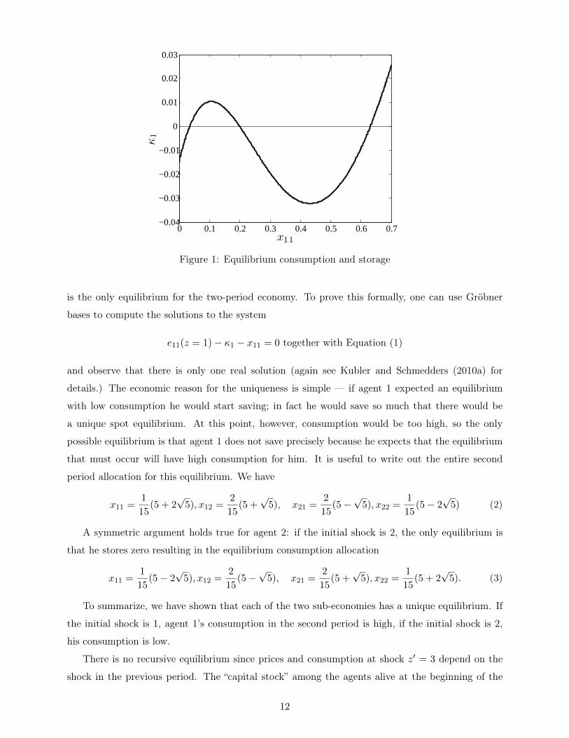
1 depicts the relation between the equilibrium consumption, x11, and κ1. The figure clearly shows
that for κ1 = 0 there are three different values of x11 that are consistent with equilibrium.
Moving to the two-period model, one obviously obtains that if the initial shock is 1, with e11(z =
1) = 115(5+2
√5) one equilibrium is κ1 = κ2 = 0, x11(z = 1) = e11(z = 1), x11(z′ = 3) = e11(z = 1).
Despite the fact that at κ1 = 0 we found 3 solutions to Equation (1) above, it turns out that this
11
0 0.1 0.2 0.3 0.4 0.5 0.6 0.7−0.04
−0.03
−0.02
−0.01
0
0.01
0.02
0.03
x11
κ1
Figure 1: Equilibrium consumption and storage
is the only equilibrium for the two-period economy. To prove this formally, one can use Gröbner
bases to compute the solutions to the system
e11(z = 1)− κ1 − x11 = 0 together with Equation (1)
and observe that there is only one real solution (again see Kubler and Schmedders (2010a) for
details.) The economic reason for the uniqueness is simple — if agent 1 expected an equilibrium
with low consumption he would start saving; in fact he would save so much that there would be
a unique spot equilibrium. At this point, however, consumption would be too high, so the only
possible equilibrium is that agent 1 does not save precisely because he expects that the equilibrium
that must occur will have high consumption for him. It is useful to write out the entire second
period allocation for this equilibrium. We have
x11 =1
15(5 + 2
√5), x12 =
2
15(5 +
√5), x21 =
2
15(5−
√5), x22 =
1
15(5− 2
√5) (2)
A symmetric argument holds true for agent 2: if the initial shock is 2, the only equilibrium is
that he stores zero resulting in the equilibrium consumption allocation
x11 =1
15(5− 2
√5), x12 =
2
15(5−
√5), x21 =
2
15(5 +
√5), x22 =
1
15(5 + 2
√5). (3)
To summarize, we have shown that each of the two sub-economies has a unique equilibrium. If
the initial shock is 1, agent 1’s consumption in the second period is high, if the initial shock is 2,
his consumption is low.
There is no recursive equilibrium since prices and consumption at shock z′ = 3 depend on the
shock in the previous period. The “capital stock” among the agents alive at the beginning of the
12
period plays no role and is in fact zero in equilibrium, prices rather being determined by the previous
shock. If the economy is in shock 1, agent 1 is rich and he decides not to save for next period’s
shock 3 only if he expects equilibrium prices of good 2 to be high, i.e., he expects his consumption
to be high. If he were to expect the equilibrium that is bad for him (i.e., with low consumption) he
would start saving so much that the “bad” equilibrium disappears. Thus the only possible outcome
in shock 3 is the good equilibrium. If, on the other hand, the economy is in shock 2, agent 2 is rich
and the same argument applies. In shock 3 each agent’s consumption depends on his endowments
in the previous period, not because of savings but because of expectations.
4 Existence
In this section we prove the existence of a recursive equilibrium. Section 4.1 shows how to char-
acterize recursive equilibrium via marginal utility functions. Section 4.2 proves existence making
direct assumptions on the transition probability for the recursive state. Assumptions on economic
fundamentals that guarantee these conditions are provided in Section 4.3.
4.1 Characterizing recursive equilibria
We now characterize recursive equilibrium via a function that maps the recursive state into marginal
utilities of all agents. We show that such a function describes a recursive equilibrium if it is a fixed
point of an operator that captures the period-to-period equilibrium conditions.
We make the following assumption on preferences and endowments:
Assumption 1
1. Endowments are bounded above and below: There are ω, ω ∈ R+ with ω > 0 such that for all
shocks z, all goods l, and all agents h
ω < ωhl(z) < ω.
2. The agents’ discount factors satisfy δ ∈ (0, 1).
3. The Bernoulli functions uh : Z × RL++ → R are assumed to be measurable in z and strictly
increasing, strictly concave, and C2 in x. They satisfy a strong Inada condition: for each z ∈ Z
and all x ∈ RL+ \ RL++ along any sequence xn → x, uh(z, xn) → −∞. Moreover, utility is
bounded above in the sense that there exists a u such that for all h ∈ H, uh(z, x) ≤ u for all
z ∈ Z, x ∈ RL++.
The assumption that all commodities enter an agent’s utility function is made for convenience and
can be relaxed. Similarly, the assumption that individual endowments are strictly positive in all
13
commodities is very strong, but can be replaced by an alternative assumption. We discuss these
assumptions in Section 5.2.
As in Duffie et al. (1994), Assumption 1 implies that there is a c > 0 such that, independently
of prices, an agent will never choose consumption that is below c in any component, i.e. xl(st) ≥ c
for all commodities l whenever (x(st)) is an optimal consumption process for any agent. The reason
is that an agent can always consume his endowments (he cannot sell them on financial markets in
advance), and we therefore must have, for any shock z and for any x that is sufficiently small in
one component,
uh(z, x) +δu
1− δ< uh(ωh(z)) + Ez
[ ∞∑t=1
δtuh(ωh(zt))
],
where u is the upper bound on Bernoulli utility.
We therefore define
C = {x ∈ RL+ : xl ≥ c for all l = 1, ..., L}.
The lower bound on consumption implies an upper bound on marginal utility, which we define by
m = maxh∈H
supx∈C,z∈Z
‖Dxuh(z, x)‖∞.
We make the following assumptions on production possibilities:
Assumption 2 For each shock z the production set Y(z) ⊂ RL is assumed to be closed, convex-
valued, to contain RL−, exhibit constant returns to scale, i.e., y ∈ Y(z)⇒ λy ∈ Y(z) for all λ ≥ 0, and
to satisfy Y(z) ∩ −Y(z) = {0}. In addition, production is bounded above: There is a κ ∈ R+ so that
for all κ ∈ KU , h ∈ H, z ∈ Z, l ∈ LK , and for all αh ∈ RJ+∑h∈H
(A0h(z)αh − κh − eh(z)
)∈ Y(z)⇒ sup
z′
∑h∈H
(fhl(z′) +
∑j∈J
a1hjl(z
′)αhj) ≤ max[κ,∑h∈H
κhl].
While the first part of Assumption 2 is standard, the second part is a strong assumption on the
interplay of intra- and inter-period production. For each capital good, the economy can never grow
above κ when starting below that limit. The assumption is made for convenience and ensures
boundedness of consumption. Stronger specific assumptions on the correspondence Y might lead
to a relaxation of the second part of the assumption.
We define
K = {κ ∈ KU :∑h∈H
κhl ≤ κ, κhl ≥ ω for all l ∈ LK and all h ∈ H} (4)
and take the state space to be S = Z×K with Borel σ-algebra S.
Define Ξ to be the set of storage decisions across agents, α, that ensure that next period’s
endogenous state lies in K, i.e.,
Ξ = {α ∈ RHJ+ :(fh(z′) +A1
h(z′)αh)h∈H∈ K for all z′ ∈ Z}.
14
Assumptions 1 and 2 allow us to give the following simple sufficient condition for the existence
of a recursive equilibrium.
Lemma 1 A recursive equilibrium exists if there are bounded functions M : S → RHL+ such that for
each s = (z, κ) ∈ S there exist prices p ∈ ∆L−1, production plans y ∈ Y(z), and optimal actions
(xh, αh) for each agent h ∈ H with Dxuh(z, xh) = Mh(s) and α ∈ Ξ such that
(xh, αh) ∈ arg maxx∈RL+,α∈RJ+
uh(z, x) + δEs[Mh(s′)A1
h(z′)α]s.t.
−p · (x− κh − eh(z) +A0h(z)α) ≥ 0
where
s′ =(z′,(A1h(z′)αh + fh(z′)
)h∈H
),
production plans are optimal, i.e.,
y ∈ arg maxy∈Y(z)
p · y,
and markets clear, i.e., ∑h∈H
(xh +A0h(z)αh − eh(z)− κh) = y.
This alternative characterization of a recursive equilibrium in terms ofM -functions is useful because
in order to show the existence it suffices to provide a fixed point argument in the space of these
marginal utility functions. This is at the heart of our existence proof below. To prove the lemma
note that if the conditions in the lemma are satisfied then there exist ((xht, αht)h∈H, pt) such that
markets clear, budget equations hold, and such that the following first order conditions hold for
each agent h ∈ H:
Dxuh(zt, x(zt))− λh(zt)p(zt) = 0 (5)
α(zt) ⊥(−λh(zt)p(zt)A0
h(zt) + Ezt[Dxuh(xh(zt+1))A1
h(zt+1)])≥ 0. (6)
To prove Lemma 1, it suffices to show that these conditions are sufficient for (xht, αht) to be a
solution to the agents’ infinite horizon problem. Although it is a standard argument we give it for
completeness. Following Duffie et al. (1994), assume that for any agent h, given prices, a budget
feasible policy (xht, αht) satisfies (5) and (6). Suppose there is another budget feasible policy
(xht, αht). Since the value of consumption in 0 only differs by the value of production plans, strict
concavity of uh(z, .) together with the gradient inequality implies that
uh(z0, xh(z0)) ≥ uh(z0, xh(z0)) +Dxuh(z0, xh(z0))A0h(z0)(αh(z0)− αh(z0)). (7)
We show by induction, that for any T, we have
E0
[ ∞∑t=0
δtuh(zt, xh(zt))
]≥ E0
[∑Tt=0 δ
tuh(zt, xh(zt))]
+ E0
[∑∞t=T+1 δ
tuh(zt, xh(zt))]
+ (8)
δTE0
[Dxuh(zT , xh(zT ))A0
h(zT )(αh(zT )− αh(zT ))].
15
We have already shown, in (7), that (8) holds for T = 0. To obtain the induction step for αj > 0, we
use the first order conditions to substitute δEzt−1
[Dxuh(zt, xh(zt))a1
hj(zt)(αhj(zt−1)− αhj(zt−1))
]for Dxuh(x(zt−1))a0
hj(zt−1)(αhj(zt−1) − αhj(zt−1)), and then apply the budget constraint and the
law of iterated expectations. When αj = 0, it is clear that αj ≥ αj and since
δEzt−1
[Dxuh(zt, xh(zt))ahj(zt−1, zt)
]≥ Dxu(x(zt−1))ahj(zt−1, 0),
the induction step follows.
The second term on the right hand side of (8) will converge to zero as T →∞ since u is bounded
above and consumption is bounded below (as functionsM are bounded above). The third term will
converge to zero because consumption is bounded below and production is bounded by Assumption
2.
4.2 A first existence result
Using the characterization of recursive equilibrium given in Lemma 1, we now prove the existence of
a recursive equilibrium by making direct assumptions on the transition probability for the recursive
state. Assuming that the probability distribution of the next period’s state varies continuously with
current actions, the operator defined by the equilibrium conditions is a non-empty correspondence
on the space of marginal utility functions. By the Fan–Glicksberg fixed-point theorem there exists
a fixed point of the convex hull of this correspondence. Making an additional assumption that is
inspired by He and Sun (2013), we can show that this implies the existence of a recursive equilibrium.
First note that the exogenous transition probability P implies, given α ∈ Ξ, a transition prob-
ability Q(.|s, α) on S: Given α across all agents, and next period’s shock z′, the next period’s
endogenous state is given by (fh(z′) +A1
h(z′)αh)h∈H
.
To prove the existence of a recursive equilibrium we first make additional assumptions directly on
Q. To state them we need the following definition from He and Sun (2013):
Given a measure space (S,S) with an atomless probability measure λ and a sub-σ-algebra G, for
any non-negligible set B ∈ S, let GB and SB be defined as {B∩B′ : B′ ∈ G} and {B∩B′ : B′ ∈ S}.
A set B ∈ S is said to be a G-atom if λ(B) > 0 and given any B0 ∈ SB, there exists a B1 ∈ GB
such that λ(B04B1) = 0.
The following assumptions are from He and Sun (2013)3 — in Section 4.3 below we give as-
sumptions on fundamentals that imply Assumption 3 and therefore ensure existence.3Assumptions 3.1. and 3.2. correspond to the assumptions made by He and Sun (2013) on the transition probability
representing the law of motion of the states. Assumption 3.3. corresponds to their crucial sufficient condition for
existence, called the “coarser transition kernel”.
16
Assumption 3
1. For any sequence αn ∈ Ξ with αn → α0 ∈ Ξ
supB∈S|Q(B|s, αn)−Q(B|s, α0)| → 0.
2. For all (s, α), Q(.|s, α) is absolutely continuous with respect to some fixed probability measure on
(S,S), λ, with Radon–Nikodym derivative q(.|s, α).
3. There is a sub σ-algebra G of S such that S has no G atom and q(.|s, α) and A1(.) are G-measurable
for all s = (z, κ) and all α ∈ Ξ.
The first existence result of this paper is as follows:
Theorem 1 Under Assumptions 1–3 a recursive equilibrium exists.
To prove the result let M be the set of all measurable functions M : S → RHL+ that are λ-
essentially bounded above by m and below by 0. They lie in the space Lm∞(S,S, λ) of essentially
bounded and measurable (equivalence classes of) functions from S to Rm with m = HL. Fol-
lowing Nowak and Raghavan (1992) and Duggan (2012), we endow Lm∞ with the weak* topology
σ(Lm∞, Lm1 ). The set M is then a non-empty, convex, and compact subset of a locally convex, Haus-
dorff topological vector space. Moreover, since S is a separable metric space, Lm1 is separable, and
consequently M is metrizable in the weak* topology. We can therefore work with sequences rather
than nets of functions in M.
Given any M = (M1, . . . , MH) ∈M, we define
EMh (s, x, α, α∗) = uh(z, x) + δEs[Mh(s′) ·A1
h(z′)α]
(9)
with
s′ =(z′,(fh(z′) +A1
h(z′)α∗h)h∈H
).
In the definition of EMh , the α ∈ R+ stands for the choice of agent h, while the vector α∗ ∈ RH+is taken by individuals as given, in particular its influence on the state-transition. Lemma 2 states
properties of the function EMh that we need in Lemma 3. It is the direct analogue of Lemma 1 in
Duggan (2012).
Lemma 2 Given any M ∈ M, the functions EMh (., x, α, α∗) are measurable in s. For given s the
functions are jointly continuous in x, α, α∗ and M .
The next lemma is the key result in this subsection and it guarantees the existence of a policy that
satisfies the equilibrium conditions.4
4In our setup this result plays the same role as the result that there always exists a mixed strategy Nash equilibrium
for the stage game in the stochastic game setup.
17
Lemma 3 For each M ∈ M and s = (z, κ) ∈ S there exists a x ∈ RHL+ , α ∈ Ξ, y ∈ Y(z) and
p ∈ ∆L−1 such that ∑h∈H
(xh − eh(z)− κh +A0h(z)αh) = y, (10)
for each agent h
(xh, αh) ∈ arg maxx∈C,α∈RJ+
EMh (s, x, α, α) s.t. (11)
−p · (x− eh(z)− κh +A0h(z)α) ≥ 0,
and
y ∈ arg maxy∈Y(z)
p · y. (12)
Proof.
Given s ∈ S, define compact sets
A = {α ∈ RJ+ : fhl(z′) +
∑j∈J
a1hlj(z
′)αj ≤ κ for all h ∈ H, l ∈ L and all z′ ∈ Z}, (13)
C(s) = {x ∈ C :1
2x−
∑h∈H
(eh(z) + κh) ∈ Y(z)},
and
Y(s) = {y ∈ Y(z) : y +∑h∈H
(eh(z) + κh) ≥ 0}.
To ensure compactness of A it is without loss of generality to assume that for each agent h there is
a commodity l and a shock z′ such that∑
j∈J a1hlj(z
′) > 0.
Define for each agent h
Φh : ∆L−1 ×Ξ ⇒ C(s)×A
by
Φh(p, α∗) = arg maxx∈C(s),α∈A
EMh (s, x, α, α∗) s.t.
−p · (x− eh(z)− κh +A0h(z)α) ≥ 0
By a standard argument, the correspondence Φ is convex-valued, non-empty valued, and upper-
hemicontinuous. Define the producer’s best response ΦH+1 : ∆L−1 ⇒ Y(s) by
ΦH+1(p) = arg maxy∈Y(s)
p · y
and define a price player’s best response,
Φ0 : (C(s)×A)H × Y(s) ⇒ ∆L−1
by
Φ0((xh, αh)h∈H, y) = arg maxp∈∆L−1
p ·
(y −
∑h∈H
(xh − eh(z)− κh +A0h(z)αh)
).
18
It is easy to see that this correspondence is also upper-hemicontinuous, non-empty, and convex
valued. Finally, define
ΦH+2 : AH ⇒ Ξ
by
ΦH+2(α∗) = arg minα∈Ξ‖α− α∗‖2.
By Kakutani’s fixed point theorem there exists a fixed point to the correspondence XH+2h=0 Φh, which
we denote by (x, α, y, α∗, p). By a standard argument, we must have∑h∈H
(xh − eh(z)− κh +A0h(z)αh) = y.
Therefore consumption solves the agent’s problem for all x ∈ C — the upper bound imposed by
requiring x ∈ C(s) will never bind. Production maximizes profits among all y ∈ Y(z) since the
upper bound can also never bind. In addition, Assumption 2 implies that the upper bound on
each αh cannot be binding — if it were some agents would consume below c in some commodities.
Therefore each agent maximizes utility subject to x ∈ C, α ∈ RJ+. �
We can define correspondences s⇒ NM (s) to contain all (xh)h∈H such that there exist (αh)h∈H ∈
Ξ, p ∈ ∆L−1 and y ∈ Y(z) that satisfy Equations (10), (11), and (12) and s ⇒ PM (s) by
PM (s) = {(Dxuh(z, xh))h∈H : x ∈ NM (s)}. We define co(PM ) by requiring co(PM )(s) to be the
convex hull of PM (s). Let R(M) be the set of (equivalence classes of) measurable selections of PM ,
and co(R(M)) the set of measurable selections of co(PM ). In the next lemma we consider the cor-
respondence co(R) : M ⇒ M defined by co(R)(M) = co(R(M)) and establish that it has a closed
graph and non-empty, convex values. The lemma is almost directly from Nowak and Raghavan
(1992) — we include a detailed proof for completeness.
Lemma 4 For each M ∈M the correspondence PM (s) is measurable and compact valued and the cor-
respondence co(R) : M ⇒ M is non-empty, convex, weak* compact valued, and upper-hemicontinuous.
Proof.
For given s ∈ S the set of allocations x ∈ RHL+ , α ∈ Ξ, y ∈ Y (z), and prices p ∈ ∆L−1 satisfying
(10), (11), and (12) can be described as solutions to a system of equations and inequalities. It is
easy to notice that the correspondence mapping s to equilibrium allocations and prices, s⇒ NM (s),
is non-empty and compact-valued. Simplifying, the correspondence can be written in the following
way:
NM (s) ={x ∈ X : f(s, x) = 0, g(s, x) ≥ 0} ∩ X(s)
={x ∈ X : g(s, x) = 0} ∩ {x ∈ X : g(s, x) ≥ 0} ∩ X(s)
19
where the functions f and g are Caratheodory, and X(s) is lower measurable and compact valued.
Moreover, since production is bounded above and endowments are bounded (see Assumptions 1
and 2), we can choose X to be compact. By Corollary 18.8 in Aliprantis and Border (2006) the
correspondence s ⇒ {x ∈ X : f(s, x) = 0} is measurable. The map s ⇒ {x ∈ X : g(s, x) ≥ 0}
is closed-valued and also measurable by Lemma 18.7, Corollary 18.8, and Lemma 18.4 (1) therein:
{x ∈ X : g(s, x) ≥ 0} = {x ∈ X : g(s, x) = 0} ∪ {x ∈ X : g(s, x) < 0}. By Lemma 18.4 (3) we get
the measurability of the correspondence s ⇒ NM (s), and hence also of s ⇒ PM (s) by continuity
of the functions Dxuh.
By the selection theorem of Kuratowski and Ryll-Nardzewski, PM has a measurable selector (see
Theorem 18.13 in Aliprantis and Border(2006)). Consequently, the map M ⇒ co(R)(M) is non-
empty valued, and obviously it is also convex-valued. Take Mn →M as n→∞, Mn,M ∈M and
vn → v such that vn ∈ co(R)(Mn) for each n. We assume that both sequences converge in the
weak* topology σ(Lm∞, Lm1 ) on the space M. We need to show v ∈ co(R)(M). Notice that for given
s, M ⇒ PM (s) has a closed graph and that Theorem 17.35 (2) in Aliprantis and Border (2006)
implies the correspondence M ⇒ co(PM (s)) has a closed graph as well. Moreover, there exists a
sequence vn of finite convex combinations of {vp : p = 1, 2, ...} such that vn converges to v almost
surely, i.e., vn(s)→ v(s) for every s ∈ S \ S1 where the set S1 is of measure zero. Given the closed
graph of M ⇒ co(PM (s)) it is now easy to show that v(s) ∈ co(PεM (s)) for any ε-neighborhood of
co(PM (s)), ε > 0, and any s ∈ S − S1. This proves that M ⇒ co(R)(M) is upper-hemicontinuous.
Similarly it can be shown that M ⇒ co(R)(M) is closed-valued and thus by compactness of M,
co(R) is weak* compact valued. �
To complete the proof of the existence of a recursive equilibrium, i.e., the proof of Theorem 1,
we apply the argument from He and Sun (2013).
Given a measure space (S,S) with an atomless probability measure λ and a sub-σ-algebra G,
and an integrably bounded and closed valued correspondence,
F : S ⇒ Rm
define co(F ) pointwise by requiring co(F )(s) to be the convex hull of F (s) and
IS,GF = {E [f |G] : f is an S-measurable selection of F}.
Dynkin and Evstigenev (1976) prove the following result:
Lemma 5 If S has no G-atom, then IS,GF = IS,Gco(F ).
Lemma 4 and the Fan–Glicksberg fixed point theorem imply that there exists a M ∈ M such
that M ∈ co(R)(M). Assumption 3 and Lemma 5 imply that there is a sub-σ-algebra G of S such
that there is a M∗ ∈ R(M) such that E [M∗|G] = E[M |G
]. Therefore we must have for each agent
20
h and all (s, α) that∫SM∗h(s′)A1
h(z′)dQ(s′|s, α) =
∫SM∗h(s′)A1
h(z′)q(s′|s, α)dλ(s′) =
∫SE[M∗hA
1h(z′)qs,α|G
]dλ
=
∫SE [M∗h |G]A1
h(z′)qs,αdλ =
∫SE[Mh|G
]A1h(z′)qs,αdλ
=
∫SMh(s′)A1
h(z′)dQ(s′|s, α).
It is then clear that for all s, PM (s) = PM∗(s) and M∗ must be a S-measurable selection
of PM∗(s). We can now construct a “constrained” recursive equilibrium from M∗, which is a
competitive equilibrium where agents are constrained to choose consumption in C. As we argued
above, it will never be optimal to choose consumption below c — by convexity we obtain the same
equilibrium if agents are choosing consumption in RL+ and hence have proven the existence of a
recursive equilibrium.
4.3 A second existence theorem
So far, we have shown the existence of a recursive equilibrium under Assumptions 1–3. However,
Assumption 3 is not on fundamentals, but on the transition probability Q for exogenous and en-
dogenous states. We now provide assumptions on fundamentals that guarantee Assumption 3 and
thus the existence of a recursive equilibrium.
In particular, we now assume that the space of exogenous shocks can be decomposed into three
complete, separable metric spaces, Z = Z0 ×Z1 ×Z2 with Borel σ-algebra Z = Z0 ⊗Z1 ⊗Z2, and
the shock is given by z = (z0, z1, z2). Moreover, for each i = 1, 2, 3 there is a measure µzi on Zi and
there are conditional densities rz0(z1|z, z′1), rz1(z′1|z), and rz2(z′2|z, z′0, z′1) such that for any B ∈ Z
we have
P(B|z) =
∫Z1
∫Z0
∫Z2
1B(z′)rz2(z′2|z, z′0, z′1)rz0(z′0|z, z′1)rz1(z′1|z)dµz2(z′2)dµz0(z′0)dµz1(z′1).
To ensure continuity of the state-transition in Assumption 3.1, we assume that the shock z0 is
purely transitory, has a continuous density, and only affects agents’ f -endowments. Moreover, given
z2 and z3, there is a diffeomorphism from Z0 to a subset of K. More precisely, we make the following
assumptions:
Assumption 4
1. z0 is purely transitory, i.e., for all z0, z0 ∈ Z0 and all (z1, z2) ∈ Z1 × Z2,
P(.|z0, z1, z2) = P(.|z0, z1, z2).
2. Z0 is a Euclidean space, µz0 is Lebesgue, and the density rz0(.|z, z′1) is continuous for (almost) all
(z, z′1) and vanishing at the boundary of its support in Z0.
21
3. For each agent h, and all (z1, z2) ∈ Z1×Z2, fh(., z1, z2) is a diffeomorphism from Z0 to a subset
of K with a non-empty interior. All other fundamentals are independent of z0, i.e., for all h, we
can write eh(z) = eh(z1, z2), A1h(z) = A1
h(z1, z2), uh(z, .) = uh((z1, z2), .), Y(z) = Y(z1, z2).
Assumption 4.3. can be slightly relaxed in that we can allow A1h(z) to depend on z0 if we assume
that for all α ≥ 0, fh(., z′1, z′2) +A1
h(., z′1, z′2)α is a diffeomorphism from Z0 to a subset of RHL. For
simplicity we take A1h(.) to be independent of z0.
To ensure that the z2 shock ensures convexity in the conditional expectation operator we make
the following assumption:
Assumption 5 Conditionally on next period’s z′1 the shock z′2 is independent of both z′0 and the current
shock z, i.e., we can write rz2(z′2|z, z′0, z′1) = rz2(z′2|z′1). The measure µz2 is an atomless probability
measure on Z2 and, for each agent h, A1h(z) and fh(z) do not depend on z2.
This construction was first used in Duggan (2012). It is clear that this is a strict generalization of
a “simple sunspot”. The shock z2 can affect fundamentals (eh)h∈H and Y in arbitrary ways.
The following is the main result of the paper.
Theorem 2 Under Assumptions 1, 2, 4, and 5 there exists a recursive equilibrium.
To prove the theorem we show that Assumptions 4 and 5 imply Assumption 3 if state-transitions
and the state space are reformulated appropriately. It is easy to notice that since the shock z0 is
purely transitory and does not affect any fundamentals except (fh), the realization of this shock
is reflected in the value of the endogenous state κ and except for the value of κ it is irrelevant for
current endogenous variables and the future evolution of the system. Therefore, departing slightly
from our previous notation, we take S = Z1 × Z2 ×K with Borel σ-algebra S. Furthermore we
write S = Z1 ×K for the space that includes only the z1- shock component and the holdings in
capital goods; we denote the Borel σ-algebra of S by S. For each B ∈ S take
Q(B|s, α) = P({z′ ∈ Z :
((z′1, z
′2), (fh(z′) +A1
h(z′)αh)h∈H
)∈ B}|z
).
We have the following lemma:
Lemma 6 Under Assumpion 4 , Q(.|s, α) satisfies Assumption 3.1.
Proof. By Assumption 5, it suffices to show norm-continuity for the marginal transition function
on S, i.e., that for any sequence αn ∈ Ξ with αn → α0 ∈ Ξ
supB∈S|Qs(B|s, αn)−Qs(B|s, α0)| → 0.
To show this, we first define for given (z, z′1) ∈ Z × Z1 and α ∈ Ξ a diffeomorphism g(z,z′1,α) that
maps Z0 into its range K(z,z′1,α) = g(z,z′1,α)(Z0) ⊆ K with g(z,z′1,α)(z0) = (fh(z′0, z′1) +A1
h(z′1)αh)h∈H
22
and
rκ(κ′|z, z′1, α) :=
rz0(g−1(z,z′1,α)
(κ′)|z, z′1) ·∣∣∣J(g−1
(z,z′1,α)(κ′))
∣∣∣ if ∃ z0 : g(z,z′1,α)(z0) = κ′
0 otherwise,
where |J(·)| denotes the determinant of the Jacobian.
Denoting by µκ the Lebesgue measure on K, for B ∈ S and αn ∈ Ξ with αn → α0 ∈ Ξ, we have
Qs(B|s, αn) =
∫Z1
∫Z0
1B
[z′1, (fh(z′) +A1
h(z′)αnh)h∈H
]rz0(z′0|z, z′1)rz1(z′1|z)dµz0(z′0)dµz1(z′1)
=
∫Z1
∫Z0
1B
[z′1, g(z,z′1,α
n)(z′0)]rz0(z′0|z, z′1)rz1(z′1|z)dµz0(z′0)dµz1(z′1)
=
∫Z1
∫K(z,z′1,α
n)
1B
[z′1, κ
′] rκ(κ′|z, z′1, αn)rz1(z′1|z)dµκ(κ′)dµz1(z′1)
=
∫Z1
∫K1B
[z′1, κ
′,]rκ(κ′|z, z′1, αn)rz1(z′1|z)dµκ(κ′)dµz1(z′1)
=
∫Brκ(κ′|z, z′1, αn)rz1(z′1|z)dµκ(κ′)dµz1(z′1),
where we used Fubini’s theorem for the first equality and the change of variables theorem for the
third equality. By Scheffe’s lemma and the convergence rκ(κ′|z, z′1, αn) → rκ(κ′|z, z′1, α0), we get
norm-continuity of α→ Qs(·|s, α). �
In the above proof, we have shown that for all (s, α) the marginal distribution of Q(.|s, α) on S is
absolutely continuous with respect to the product measure η = µκ×µz1 and has a Radon–Nikodym
derivative qs(z′1, κ′|s, α) = rκ(κ′|z, z′1, α)rz1(z′1|z).
The following result is directly from He and Sun (2013), Proposition 4.
Lemma 7 Defining the measure λ(.) by
λ(B) =
∫S
∫Z2
1B[s, z2]rz2(z2|z1)dµz2(z2)dη(s)
and taking G = S ⊗ {∅,Z2}, Assumption 5 implies that Q(.|s, α) satisfies Assumptions 3.2 and 3.3.
The proof of Theorem 2 now follows directly from the argument above, i.e., the result follows
directly from Theorem 1.
4.4 The examples revisited
Assumption 5 and especially Assumption 4 are strong assumptions regarding the underlying econ-
omy. Assumption 4 guarantees that agents’ current choices lead to a non-degenerate distribution
over the endogenous state next period, conditional on the exogenous shock. This is in contrast
with standard models where current choices often pin down next period’s endogenous state deter-
ministically. In stochastic games it is well known that the assumption of a so-called deterministic
transition creates serious problems for the existence of Markov equilibria (see Duggan (2012) for
23
an explanation and in particular Levy (2013) for an example of non-existence in a model with a
deterministic transition). We want to argue that our examples from Section 3 above show that the
same is true in general equilibrium models and that it is not possible to expect a general existence
result without some form of continuity in the state-transition.
The situation is slightly complicated by the fact that our stylized examples of non-existence
violate Assumption 1, Assumption 4, and Assumption 5 above. However, it is easy to see that
Assumption 1 alone cannot restore existence in the examples. In particular, Example 2 goes through
if endowments are in the interior of the consumption set; the specific endowments were simply chosen
to make the examples as simple as possible. It is much more difficult to determine whether both
Assumptions 4 and 5 are necessary for obtaining general existence.
In particular Assumption 5 alone guarantees existence in Example 2 and in any simple pertur-
bation of Example 2. To see this, we modify the example slightly and assume that the shock has a
continuous component, Z = {1, 2, 3} × [0, 1]. Endowments, technology, and Bernoulli utility in the
discrete shocks 1 and 2 do not depend on ζ ∈ [0, 1], the continuous component of the shock. The
same is true for Bernoulli utilities in the discrete shock 3, however endowments are now as follows
e1(z = (3, ζ)) = (0, 1 + ζζ), e2(z = (3, ζ)) = (1 + ζζ, 0) for some ζ ≥ 0.
To simplify the analysis we also assume that ζ affects inter-period production — this is not consistent
with Assumption 5, but this plays no role in our example. We assume that a11(3, ζ) = (1 + ζζ, 0)
and a21(3, ζ) = (0, 1 + ζζ).
Note that for ζ = 0 the additional exogenous shock is a pure sunspot not affecting economic
fundamentals but possibly playing the role of a coordination device since in equilibrium agents can
base their decisions on the realization of this shock. We show that both for ζ = 0 and for ζ > 0 the
additional shock restores existence.
Clearly there is still a sequential competitive equilibrium where spot-prices depend on the re-
alization of the shock in the previous period and agents never save. By homotheticity of utilities
each shock (z = 3, ζ) just scales the economy: given storage, equilibrium prices are all identical and
consumption just shifts up. However, if we allow spot prices to change with the realization of the
shock, as is the case in the definition of recursive equilibrium, it is easy to obtain the existence of a
recursive equilibrium. The construction is as follows:
Without loss of generality we focus on the case where shock 1 occured in the previous period and
agent 2 does not save, so κ1 ≥ 0, κ2 = 0. Denote by x11 = 115(5− 2
√5) the smallest real solution of
Equation (1) at κ1 = 0 and by x11 ∼ 0.6609 the largest real solution of that equation at κ1 = 0.01.
For each κ1 ∈ [0, 0.01] define η(κ1) as a unique solution in [0, 1] of the following equation
η(κ1)1
x3L
+ (1− η(κ1))1
x3H
=1
x113
+κ1
0.01
(1
x113 −
1
x113
),
24
where xL is the smallest and xH is the largest solution to Equation (1) at κ1. The policy functions
in a recursive equilibrium are then as follows: given κ1 if 0 ≤ ζ ≤ η(κ1) agent 1 consumes (1+ζζ)xL
and if η(κ1) < ζ ≤ 1 agent 1 consumes (1 + ζζ)xH .
It can easily be verified that expected marginal utility is a continuous and decreasing function
in κ1 and that there always exists a solution for the optimal savings in shock 1. Since shock 2 is
completely symmetric there exists a recursive equilibrium.
Since in many applied models Assumption 5 is likely to be much weaker than Assumption 4, the
fact that this assumption alone guarantees existence in our Example 2 is an important observation.
However, note that the assumption does not suffice for existence in Example 1 — even a pure
sunspot cannot help agents to coordinate if κ1 = κ2 = 0 and recursive equilibrium does not exit.
The reason is simple — in Example 2 the equilibrium correspondence in shock 3 (equilibrium prices
and allocations as a map from (κ1, κ2)) is not convex valued, thus introducing a continuous shock
allows us to convexify the correspondence and find a continuous selection. In Example 1 this
correspondence is convex valued to begin with. But there is no continuous selection and hence a
continuous shock cannot restore existence.
Assumption 5 cannot restore existence in cases where the convex hull of the equilibrium corre-
spondence does not admit a continuous selection. In the class of examples considered in Section
3 this is only possible for non-generic economies (since it requires indeterminacy of equilibria in a
static economy) but there is no reason to believe that in a full-fledged dynamic economy this is also
the case.
Assumption 4, on the other hand, does guarantee existence in both Examples 1 and 2. It
guarantees that Lemma 2 holds and this is sufficient to establish existence in simple examples where
the infinite horizon economy decomposes into two-period economies. Existence in the two examples
fails precisely because EM (s, x, α, α∗) is never continuous in α∗ if M is not continuous itself. But it
is easy to see that in both Example 1 and Example 2 the map from (κ1, κ2) to equilibrium marginal
utilities in shock 3 does not have a continuous selection. Given any measurable selection, a version of
Assumption 4 guarantees continuity of EM and the existence of a recursive equilibrium. Concretely,
it suffices to assume in both examples that conditional on shock 3, the joint distribution of agent 1’s
endowments in commodity 1 and agent 2’s endowments in commodity 2 is uniform on [0, ε]2. While
this does not exactly satisfy Assumption 4 (e.g., the density of the shock to agents’ f -endowments
does not vanish at the boundary), one can verify that it guarantees continuity of EMh (s, x, α, α∗) in
α∗ for any (measurable) selection M of the equilibrium correspondence in shock 3 (i.e., the map for
κ to consumptions and marginal utilities).
To summarize, the failure of existence in the examples in Section 3 stems from the fact that
these examples violate Assumption 4. While in simple examples existence might be restored without
assuming continuity of the transition, the examples demonstrate that in general one cannot expect
25
existence without a form of Assumption 4. The examples do not show why Assumption 5 is necessary
for existence but it is clear that our proof critically relies on convexity, which cannot be obtained
without Assumption 5. Whether or not existence of Markov equilibria can be shown with a different
approach and without Assumption 5 is subject to further research.
5 Extensions
So far, we have considered the case without trade in one-period financial assets. In this section, we
describe a simple way of incorporating financial markets into our framework. We also discuss an
alternative formulation of Assumption 1 that might be more suitable for some applications.
5.1 Financial markets
We now assume that agents can trade in financial markets, in addition to undertaking intertemporal
storage. There are D one-period securities, d = 1, ..., D, in zero net supply, each being characterized
by its payoff bd : Z→ RL+ — a bounded and measurable function of the shock. At each zt securities
are traded at prices ρ(zt); we denote an agent’s portfolio by θh(zt) ∈ RD.
In order to establish the existence of a recursive equilibrium we need to restrict agents’ portfolio
choices. Let K be defined as in (4) above and A as in (13). Each agent h faces a constraint on trades
in asset markets and storage decisions (α, θ), given by a convex and closed set Θh ⊂ RJ+ × RD,
which satisfies that whenever α ∈ A and (α, θ) ∈ Θh then
A1h(z′)α+
D∑d=1
θdbd(z′) ≥ 0 for all z′ ∈ Z.
Without loss of generality we assume that trade is possible in all financial securities, i.e., for each d
there is an agent h and an α ∈ A so that for some θd < 0, (α, θ) ∈ Θh.
Note that collateral constraints of the form
A1h(z′)α+
D∑d=1
min(θd, 0)bd(z′) ≥ 0 for all z′ ∈ Z,
are one example of constraints that satisfy our assumption, but there could be many others. How-
ever, this is a somewhat nonstandard formulation of a collateral constraint since agents cannot
borrow against the value of their future production — they need to borrow against future produc-
tion directly.
As before the endogenous state-space is given by K. A recursive equilibrium is given by maps
from the state s ∈ S = Z×K to prices of commodities and financial securities as well as consumption,
investment, and portfolio choices across all agents. The analogous result to Lemma 1 above is now
as follows:
26
A recursive equilibrium exists if there are functions M : S → RHL+ such that for each s ∈ S
there exist prices (p, ρ) ∈ ∆D+L−1, a production plan y ∈ Y(z) for each agent h, optimal actions
(xh, αh, θh) with Dxuh(xh) = Mh(s), and
(xh, αh, θh) ∈ arg maxx∈RL+,(α,θ)∈Θh
uh(z, x) + δEs
Mh(s′) ·
∑j
a1hj(z
′)αj +∑d
bd(z′)θd
s.t.
−q · θ − p · (x− κh − eh(z) +A0h(z)α) ≥ 0,
where
s′ =
z′,(A1h(z′)αh +
∑d
θhdbd(z′) + fh(z′)
)h∈H
,
production plans are optimal, i.e.,
y ∈ arg maxy∈Y(z)
p · y,
and markets clear, i.e., ∑h∈H
(xh +A0h(z)αh − eh(z)− κh) = y
and ∑h∈H
θh = 0.
The proof is similar to the proof of Lemma 1.
Assumptions 4.3 and Assumption 5 now need to be extended in that we assume in addition that
for each asset d, bd(z) does not depend on z0 and does not depend on z2, i.e., it is only a function
of z1. The definition of the transition probability Q now reads as
Q(B|s, α, θ) = P
({z′ ∈ Z : [z′1, z
′2, (fh(z′) +A1
h(z′)αh +∑d
θhdbd(z′))h∈H] ∈ B}|z
).
With the additional assumptions, it is easy to see that Lemma 6 holds as stated. The proofs of
Lemma 2 and 4 are almost identical as those in the case without financial securities. To prove the
analogue of Lemma 3, one can bound the set of admissible portfolios, and proceed as in the proof
in Section 4.
5.2 Assumptions on endowments and preferences
Standard formulations of both the Lucas asset pricing model and the neoclassical stochastic growth
model violate our Assumption 1. Agents are not endowed with capital or Lucas trees and they do
not derive utility from consuming them.
The first part of the assumption, ωh(z) ∈ RL++, cannot be relaxed easily since we need to require
positive f -endowments in order to guarantee Assumption 3.1. However, while they have to be
27
positive, f -endowments can be arbitrarily small. Therefore, this assumption can be interpreted as
a small perturbation to the original model that ensures existence. An alternative is to require that
agents operate all technologies at a positive level, i.e., to require that for some ε > 0 agents face
the additional constraint that αj ≥ ε for all j. With this alternative assumption one then needs to
make similar assumptions on A1h(z′) as we did on fh(z). In concrete examples (e.g., the neoclassical
growth model with one consumption good) this additional constraint might never be binding (e.g.,
if agents can have zero labor endowments with positive probability, then the Inada condition on
utility will always force them to have positive savings). It is beyond the scope of this paper to work
out precise conditions for existence in these cases where we allow agents’ endowments to lie on the
boundary of RL+.
The second part of the assumption, that uh(z, .) is strictly increasing in all L commodities,
seems much more problematic. However, this assumption can be substantially relaxed once one
makes concrete assumptions on the technology. Assume that utility only depends on a subset
of commodities (for example, the “consumption-goods” that cannot be obtained through storage)
LC = {1, ..., LC}, LC ≤ L, and that it is strictly increasing, strictly concave, C2, satisfies the
strong Inada condition, and is bounded as a function of these commodities. For this case, Lemma 3
needs to be slightly reformulated to ensure that the M -functions are defined even for commodities
that do not enter the utility directly: a recursive equilibrium exists if there are bounded functions
M : S→ RHL+ such that for each s ∈ S there exist prices p ∈ ∆L−1 and optimal actions (xh, αh) for
each agent h ∈ H with α ∈ Ξ such that
Dxuh(z, xh) = (Mh1(s), . . . ,MhLC (s)) and (Mh,LC+1(s), ...,Mh,L(s)) = ξh(pLC+1, . . . , pL),
with ξh = ∂uh(z,xh)/∂x1p1
and such that
(xh, αh) ∈ arg maxx∈RL+,α∈RJ+
uh(z, x) + δEs[Mh(s′)A1
h(z′)α]s.t.
−p · (x− κh − eh(z) +A0h(z)α) ≥ 0
where
s′ =(z′,(A1h(z′)αh + fh(z′)
)h∈H
),
production plans are optimal and markets clear.
The existence proof of the previous section can then be applied if assumptions on production
ensure that, in the “two-period problem”, the prices of the goods that do not enter the utility
functions are bounded below by zero and uniformly above by some constant. More precisely, in
Lemma 3 we need to require that there exist p ∈ ∆L−1 such that for each agent h and each l, it
holds that 0 ≤ ξhpl ≤ m, with ξh defined as above. For standard models, e.g., the neoclassical
growth model or the Lucas model, this can be seen to hold fairly easily.
28
References
[1] Aliprantis, C.D. and K. Border (2006), Infinite Dimensional Analysis: A Hitchhiker’s Guide.
Berlin: Springer.
[2] Brumm, J. and F. Kubler (2014), “Applying Negishi’s Method to Stochastic Models with Over-
lapping Generations,” Working Paper, University of Zurich.
[3] Citanna, A. and P. Siconolfi (2010), “Recursive Equilibrium in Stochastic Overlapping-
Generations Economies,” Econometrica, 78, 309 – 347.
[4] Citanna, A. and P. Siconolfi (2012), “Recursive equilibria in stochastic OLG economies: In-
complete markets,” Journal of Mathematical Economics, 48, 322 – 337.
[5] Duffie, D., J. Geanakoplos, A. Mas-Colell, and A. McLennan (1994), “Stationary Markov Equi-
libria,” Econometrica, 62, 745–781.
[6] Duggan, J. (2012), “Noisy Stochastic Games, ” Econometrica, 80, 2017–2045.
[7] Dumas, B. and A. Lyasoff (2012), “Incomplete-Market Equilibria Solved Recursively on an
Event Tree,” Journal of Finance, 67, 1897 – 1941.
[8] Dynkin, E.B. and I.V. Evstigneev (1977), “Regular Conditional Expectations of Correspon-
dences,” Theory of Probability and its Applications 21, 325-338.
[9] Feng, Z., J. Miao, A. Peralta-Alva and M. Santos (2014), “Numerical Simulation of Non-optimal
Dynamic Equilibrium Models, ” International Economic Review, 55, 83–111.
[10] He, W. and Y. Sun (2013), “Stationary Markov Perfect Equilibria in Discounted Stochastic
Games,” Working Paper.
[11] Heaton, J. and D. Lucas (1996), “Evaluating the effects of incomplete markets on risk sharing
and asset prices,” Journal of Political Economy, 104, 443-487.
[12] Hellwig, M. (1983), “A Note on the implementation of rational expectations equilibria,” Eco-
nomic Letters, 11, 1-8.
[13] Krebs, T. (2004), “Non-existence of recursive equilibria on compact state spaces when markets
are incomplete,” Journal of Economic Theory, 115, 134-150.
[14] Krusell, P. and A. Smith (1998), “Income and Wealth Heterogeneity in the Macroeconomy,”
Journal of Political Economy, 106(5), 867–896.
[15] Kubler, F. and H.M. Polemarchakis (2004), “Stationary Markov Equilibria for Overlapping
Generations,” Economic Theory, 24, 623–643.
29
[16] Kubler, F. and K. Schmedders (2002), “Recursive equilibria in economies with incomplete
markets,” Macroeconomic Dynamics, 6, 284-306.
[17] Kubler, F. and K. Schmedders (2003), “Stationary Equilibria in Asset-Pricing Models with
Incomplete Markets and Collateral,” Econometrica, 71, 1767-1795.
[18] Kubler, F. and K. Schmedders (2010a), “Tackling Multiplicity of Equilibria with Gröbner
Bases,” Operations Research, 58, 1037-1050.
[19] Kubler, F. and K. Schmedders (2010b), “Competitive Equilibria in Semi-Algebraic Economies,”
Journal of Economic Theory, 145, 301-330.
[20] Levy, Yehuda (2013), “Discounted Stochastic Games with no Stationary Nash Equilibrium:
Two Examples,” Econometrica, 81, 1973–2007.
[21] Lucas, R. E (1978), “Asset prices in an exchange economy,” Econometrica, 46, 1429-1446.
[22] Luenberger, D. (1969), Optimization by Vector Space Methods. Wiley Professional Paperback
Series. New York.
[23] Ljungqvist, L. and T.J. Sargent (2004), Recursive Macroeconomic Theory. MIT Press.
[24] Maskin, E. and J. Tirole (2001), “Markov Perfect Equilibrium, ” Journal of Economic Theory
100, 191-219.
[25] Nowak, R. and T. Raghavan, (1992), “Existence of Stationary Correlated Equilibria with Sym-
metric Information for Discounted Stochastic Games,” Mathematics of Operations Research,
17, 519–526.
[26] Santos, M. (2002), “On non-existence of Markov equilibria in competitive market economies,”
Journal of Economic Theory, 105, 73-98.
30