Recursive causal models

/. Austral. Math. Soc. (Series A) 36 (1984), 30-52

RECURSIVE CAUSAL MODELS

HARRI KIIVERI, T. P. SPEED and J. B. CARLIN

(Received 30 October 1981)

Communicated by R. L. Tweedie

Abstract

The notion of a recursive causal graph is introduced, hopefully capturing the essential aspects of thepath diagrams usually associated with recursive causal models. We describe the conditional indepen-dence constraints which such graphs are meant to embody and prove a theorem relating the fulfilmentof these constraints by a probability distribution to a particular sort of factorisation. The relation ofour results to the usual linear structural equations on the one hand, and to log-linear models, on theother, is also explained.

1980 Mathematics subject classification (Amer. Math. Soc): 62 F 99, 60 K 35.Keywords and phrases: causal models, path analysis, conditional independence, log-linear models.

Introduction

In his initial exposition of path analysis, Wright (1921) introduced into statisticsthe basic idea of directed graphs whose vertices represent continuous randomvariables and edges some notion of correlation and causation. Apart from simplydepicting the general nature of the linear structural equations which define thecausal relations under study, these graphs are also used to write down thosepartial correlations which must vanish when the equations and the associateddistributional assumptions take a standard form, see Blalock (1962). Furthermore,the path analysis rules of Wright (1921, 1934) involve tracing paths in the graphas part of an algorithm giving equations relating the variances and covariances ofthe random variables. More recently, Goodman (1973a, b) has drawn similargraphs whose vertices correspond to discrete random variables and edges to a

1984 Australian Mathematical Society 0263-6115/84 $A2.00 + 0.00

30

use, available at https://www.cambridge.org/core/terms. https://doi.org/10.1017/S1446788700027312Downloaded from https://www.cambridge.org/core. IP address: 65.21.228.167, on 19 Mar 2022 at 23:54:53, subject to the Cambridge Core terms of

https://www.cambridge.org/core/terms

https://doi.org/10.1017/S1446788700027312

https://www.cambridge.org/core

[2] Recursive causal models 31

notion of interaction in a probability model of the log-linear type. He has pointedout that in certain examples, these models embody conditional independenceconstraints on the distribution of the random variables.

In a different context we find that Markov fields over finite undirected graphs(that is, probability distributions for random variables identified with the verticesof such graphs which satisfy certain independence constraints defined by thegraph) have intimate connexions with the theory of log-linear models, see Dar-roch et al. (1980). A fundamental result in the theory relates Markov fields toso-called nearest-neighbour Gibbs states, and this turns out to include a descrip-tion of a large class of independence or Markov models for discrete randomvariables, see also Speed (1978). Can we do likewise with directed graphs, anddoes this tie up with path analysis?

Up until now there has been little consistency in the use of graphs in pathanalysis. Some authors include all possible edges between exogenous variables,making them undirected or bidirectional as they think appropriate, whilst othersdon't; some include undirectional edges associated with errors in the equations,whereas most authors don't do so, and so on. The difference here are partlyexplained by varying assumptions concerning the correlation structure on theexogenous variables or the errors in the equations, but there still remains adiversity of practices even when—and this is not always easy to determine—dif-ferent writers' intentions concerning these issues appear to be the same.

If a standard form of causal graph could be agreed upon, the question ofexactly which conditional independence constraints it should be regarded asembodying could then be addressed. These would not depend upon whether ornot discrete or continuous random variables were associated with the vertices.Given a satisfactory answer to this question, we would then attempt to describeall joint probability distributions which satisfy the appropriate independenceconstraints. If successful, the resulting unification of discrete and continuousmodels, together with the standardisation of terminology and fundamental resultswhich would ensue, should prove of value to those interested in defining, fitting,testing and interpreting causal probability models of data. This has been ourprogram.

In Section 2 we define what we call a recursive causal graph, hopefullycapturing the essence of the path diagrams associated with recursive causalmodels. These graphs permit neither causal cycles nor simultaneity. We describethe separation properties which help define the independence constraints thegraph is meant to embody, and our main theorem relates the fulfilment of theseconstraints by a probability distribution to a particular sort of factorisation. Thistheorem is analysed in more detail in Section 3 for Gaussian and Section 4 formultinomial distributions. The relationship of our results to the usual linear



https://doi.org/10.1017/S1446788700027312


32 Hani Kiiveri, T. P. Speed and J. B. Carlin [3]

structural equations on the one hand, and to log-linear models, on the other, isalso explained in these last two sections. A much more extensive discussion ofthese ideas with reference and illustrations can be found in Kiiveri and Speed(1982).

2. General results

Our aim in this section is to prove a general result characterising the distribu-tion of what we will be calling a recursive causal system of random variables(equivalently, a recursive causal (probability) model). Such systems (models) willalways be associated with a particular kind of graph and we begin by collectingup some preliminaries concerning these graphs.

2.1. Causal graphs. A causal graph is an ordered pair © = (F(@), £(©))consisting of a finite set F(©) = Vx(@) U Fn(@) of vertices and a finite set£(©) = £x(@) U £„(©) of edges, with vertices in Vx(Qb) being termed exogenousand those in Fn(@) endogenous; edges in Ex(®) are undirected ones, that is,unordered pairs of distinct exogenous vertices, whilst edges in £„(©) are directedones, that is, ordered pairs of distinct vertices, the second element of which is anendogenous vertex. In what follows we denote vertices by natural numbers:1,2,3,... or h, i,j; edges are unordered or ordered pairs of vertices and depictedin the usual way, namely 1 — 2 (undirected) and i -> j (directed) respectively.

EXAMPLE 1. If3,3 4,1

= {1,2}, Fn(©,) = {3,4}, £ , (0 , ) = {1 - 2},-» 4}, then ©, may be depicted as in Figure 1.

and

FIGURE 1

We will be adapting standard graph-theoretic notions to our context in whichdirected and undirected edges coexist, and it is hoped that no confusion will resultfrom so doing. A directed [undirected] chain in a causal graph © is a sequencei0, /,,. ..,im of vertices such that /,_, -» / , [ / , _ , — /,] for / = 1,2,.. .,m, and sucha chain is called a cycle if i0 = im. All of the causal graphs which we consider in



https://doi.org/10.1017/S1446788700027312



this paper are recursive, where this term means that the graph in question has nodirected cycles.

For each j G FM(©) we write Dj,= {h G F(@): h ->y}, and refer to theelements of Dj as direct causes of y; Dj U {y} is denoted by Dj. Similarly if wewrite Bj fory and the set of vertices k connected toy via a chain y ->ji~* • • • -> k,then Aj = V(®)\Bj is termed the set of vertices anterior toy £ F(©); we alsowrite Aj = AjU {j}. The undirected graph with vertices Vx(®) and edges Ex(®)will be denoted by ©x, the subgraph on the exogenous vertices. More generally,the subgraph of © defined by any subset B c F o f vertices will be denoted by(B)@; its vertices are the elements of B and its edges those in © both of whoseelements belong to B.

An important object associated with any causal graph © is what we call theunderlying undirected graph ©" which has the same set of vertices F(@") = V{®),whilst its edges £(©") are the undirected ones Ex(®) of © together with theadditional undirected ones connecting pairs of vertices between which a directededge exists in ©, that is, £(©") = Ex(®) U £„(©), where £„(©) denotes thedirected edges of © with their direction omitted.

A triple i,j and k of distinct vertices in © is said to be in configuration [>] ifi -> k,j -> k but / and j are not connected by any edge, directed or undirected.This notion, which first appeared in Wermuth (1980), plays a key role indetermining the admissible independence statements associated with a causalgraph.

If a, b and d are disjoint sets of vertices of © we say that a and b are separatedby d in ©" if any chain i — i0, it,...,im=j connecting a vertex i G a with avertex j G b necessarily intersects d. Further, we say that a, b and d are inconfiguration [>] if there is a chain in @" from an element / G a to an element

j'• E b which includes a triple i,j & d and k G d in configuration [>] in ©.Some of our induction arguments will make use of what we will call an extreme

endogenous vertex in a causal graph @, where /* G F(@) is extreme if nodirected edge /* ->y exists in £„(©). Clearly At. — K(@) for such vertices. Aneasy induction argument proves the validity of the following

LEMMA 1. Every causal graph has at least one extreme endogenous vertex.

2.2. Factorisation of joint densities. Our main result below concerns factorisa-tions of the joint density p(\,y) of an array (X; Y) = (Xh: h G Vx(@); Yy.j G Kn(©)) indexed by the vertices of a causal graph @, and it will be convenientto use certain suggestive abbreviations for joint, marginal and conditional densi-ties. (All joint distributions will be given via strictly positive densities with respectto a product measure. In fact all the examples we discuss below are either



https://doi.org/10.1017/S1446788700027312


34 Hani Kiiveri, T. P. Speed and J. B. Carlin [s 1

Gaussian or discrete (multinomial), and these conditions are then satisfied.) In

order to illustrate our abbreviations we return to Example 1.

EXAMPLE 1 (continued). Associated with the (recursive) causal graph ©, we will

have four random variables (Xu X2; Y3, Y4), the X's being termed exogenous and

the Y's endogenous variables. Our later discussion will involve the assumption of

independence of Y3 and Xx given X2 and also of Y4 and X2 given (Xv Y3); we

abbreviate the conditions to 1 ± 3 / 2 and 2 J- 4 / 1 , 3 . Similarly the factorisations

of the joint density p of the variables which are equivalent to these independence

assertions:

and

, , />{1,2,3}(*1>*2'>'3)/>{1,3.4}(*1>.);3»

p(xx,x2, y3, y4) = rP{i,3)\x\> y^)

are abbreviated to

(12)(23)(123) = —-r\— and

(2)

Finally, the factorisation which embodies both of these conditions:

p(xux2,y3,y4) = p{U2](xu x2)p3l2(y3\x2)pm 3){y4\xu y3)

is abbreviated to

(1234) = (12)(3|2)(4| 13).

This illustration should explain how our abbreviations are intended to be read.

We will be making considerable use of the notions and results concerning

Markov random fields over finite undirected graphs which can be found in

Darroch et al. (1980) and Speed (1978, 1979). A distribution (Vx) for a set of

random variables indexed by an undirected graph ®x = (Vx, Ex) is said to be

Markov over ®x if it satisfies either of the conditions:

Local Markov Condition: For each h G Vx the conditional distribution

(h | Vx\{h}) of Xh given all the Xg, g^h, coincides with (h | dh), the conditional

distribution of Xh given all Xg with g E dh = {/: {h, i) G Ex).



https://doi.org/10.1017/S1446788700027312



Global Markov Condition: For disjoint subsets a, b and d of Vx such that dseparates a from b in Vx, we have

An extension of the global Markov condition to disjoint subsets ax,.. .,am and dwith a^ and a, separated by d ( K k < / < m) is readily found to be equivalent tothe condition stated here. The general equivalence of the local and global Markovconditions over an arbitrary finite graph does not seem to be explicit in thepublished literature. It is well known for discrete random variables, where itfollows from a characterisation of all corresponding probability distributions, seeSpeed (1979) for this result (and many references to equivalent ones), while theremarks on page 194 of that paper show how to get the general result.

2.3. The main theorem. This subsection is devoted to the statement and proof ofthe main result of the paper. It is a fairly natural extension of the correspondingresult for purely undirected graphs, although it cannot go too far without somerestrictions on the type of probability densities under consideration. Each of theimportant cases—the Gaussian and the multinomial—is discussed later in thepaper, and it turns out that statement (1) of the theorem is the lead-in to areasonable parametrisation, that is, a complete description, of all such probabilitydensities in these two cases. In a sense the theorem together with Proposition 4below provides a directed analogue of the Hammersley-Clifford or NNG — Mtheorem, so-called in Speed (1979).

THEOREM. Let % be a recursive causal graph and (X; Y) a system of randomvariables indexed by the vertices of®:

(X; Y) = (Xh:hG Vx(@); Yy.j G Vn(®)).

The following are equivalent for a strictly positive joint density (V):(1) The recursive causal factorisation:(i) (Vx) is Markov over the undirected graph ®x; and(ii)

(2) The Global Markov property for causal graphs:For all families ax,a2,...,am,dofm+ 1 > 3 pairwise disjoint subsets of V

satisfying(i) U™a, U d = Vx or, for some j G Vn, U\ma,Ud = Ay,



https://doi.org/10.1017/S1446788700027312


36 Hani Kiiveri, T. P. Speed and J. B. Carlin [7]

and(ii) for 1 < k < I < m the sets ak and at are separated by d in %x or (Aj)@, as

the case may be, and are not in configuration [>] in (Aj)&u,we have

(3) As in (2) above but with the — in (i) replaced by C ;(4) The Local Markov property for causal graphs:(i) (Vx) is locally Markov over the undirected graph @x; and(ii) For allj G Vn\

As an illustration of the theorem, we return to our example.

EXAMPLE 1 (continued). We have already asserted the equivalence of thefactorisation (1234) = (12)(3|2)(4| 13) with the pair of factorisations (123) =(12)(23)/(2) and (1234) = (123)(134)/(13). These assertions—which are easilychecked directly—can now be regarded as an instance of the theorem just stated;for example, A4 = {1,2,3,4}, D4 = (1,3), whilst D4 = {1,3,4}.

REMARK. Each assertion in the statement of the theorem has essentially twoparts: one concerning (Vx) relative to ®x, and one concerning other aspects of(V) in relation to ©. The assertions concerning (Vx) and ®x are either the sameor equivalent by the basic theorem concerning Markov probabilities over undi-rected graphs referred to in Section 2.2, and will not be referred to any further inthe proof which follows.

PROOF. (1) implies (2). We do this by induction on the cardinality | Vn\ of Vn

assuming that | Vx \= p s* 1. Let us suppose that | Vn \— q = 1, that is, assume

( 0 (V) = (Vx)(p+l\Dp+l),

and suppose that at, a2,.. .,am and d satisfy (i) and (ii) of (2) with union Ap+X.To begin the proof we show that Dp+i Qa,.Ud for some /* e {l,...,m}. Ifp + 1 e d and ^ , + i Qd the result is obvious, so we consider the case when thereexists an / £ Dp+l and i £ d. For this / there is a (unique) /* such that / G ar.Now suppose that we have ay G Dp+X andy G at for / ̂ /*. Then at, a,, and d arein configuration [>] , contradicting our assumption. Hence Dp+, C a , . U</in this



https://doi.org/10.1017/S1446788700027312


18] Recursive causal models 37

case. On the other hand if p + 1 £ a,, for some /* and i E Dp+l satisfies / £ at

for / ¥= /*, we contradict the separation assumption. Hence Dp+l c at, U d inboth cases and the assertion follows.

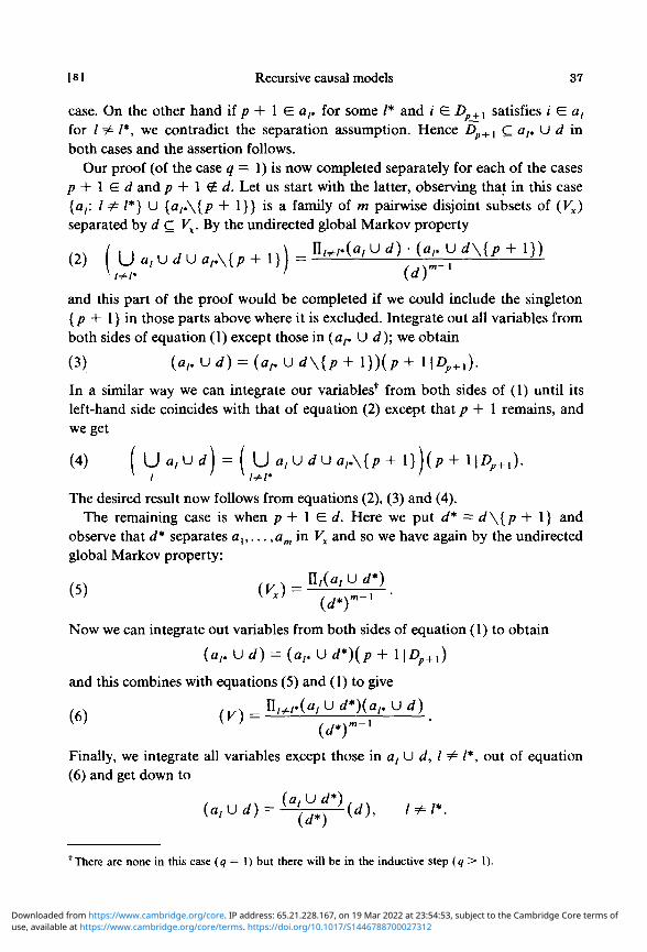
Our proof (of the case q — 1) is now completed separately for each of the casesp + 1 £ d and p + \ & d. Let us start with the latter, observing that in this case{a,: / ¥= I*} U {ar\{p + 1}} is a family of m pairwise disjoint subsets of (Vx)separated by d C Vx. By the undirected global Markov property

. . / . . i \ \ — n/=*=/•(fl/ U d) • (a/. U d\{p + 1})x I^I* (.«)

and this part of the proof would be completed if we could include the singleton{p + 1} in those parts above where it is excluded. Integrate out all variables fromboth sides of equation (1) except those in {ar U </); we obtain

(3) (a , . Ur f ) = ( a P U d\{p+ l})(p+l\Dp+l).

In a similar way we can integrate our variables* from both sides of (1) until itsleft-hand side coincides with that of equation (2) except that p + 1 remains, andwe get

(4) ( U « ( U i ) = ( \J a,U dU a,.\{p + ityp + l\Dp+x).

The desired result now follows from equations (2), (3) and (4).The remaining case is when p + 1 £ d. Here we put d* = d\{p + 1} and

observe that d* separates a,,... ,am in Vx and so we have again by the undirectedglobal Markov property:

(5) (Vx) = I['("a'Um

dP •

Now we can integrate out variables from both sides of equation (1) to obtain

(ai.Ud) = (arUd*)(p+l\Dp+l)

and this combines with equations (5) and (1) to give

nMa,^d*)(al.Ud)

(d*rl

Finally, we integrate all variables except those in a, U d, I ¥= /*, out of equation(6) and get down to

+ There are none in this case (q = 1) but there will be in the inductive step (q > 1).



https://doi.org/10.1017/S1446788700027312


38 Hani Kiiveri, T. P. Speed and J. B. Carlin [91

This, together with equation (5), gives us what we want. Thus the inductionargument has begun.

Suppose now that the implication has been proved for all recursive causalgraphs © having | Vn\< q vertices, q > 1, and let us consider such a graph with| Vn | = q. Take an extreme endogenous vertexy* £ V{%) and consider the smallergraph ©* with j * and its incident edges removed from %. This satisfies ourinduction hypothesis, and we now prove the induction step in much the same waythat the induction argument was begun. For this reason we present the argumentonly in outline.

Given a system ax,...,am, d satisfying (i) and (ii) of (2) in the statement withU, a, U d — Aj, we first note that if j * £ Aj, then the result follows from ourinductive hypothesis. Thus we need only consider the casey* £ Aj, and here wereadily observe that / £ Aj also holds for all i £ Dj, that is, that D}, C Aj. Anearlier argument now proves that Dj. c a,» U d for a unique /*, and the first partof this proof is indicated.

The remainder of the proof of the induction step goes as before. If j * £ d thenthe {a,, I ¥= / * } , fl/«\{./*} a n d d satisfy the conditions (i) and (ii) of (2) in ©* andthe induction hypothesis together with the earlier argument completes the proof.On the other hand, if j * £ d, then {at: I ~ 1 , . . . ,m) and d* = d\{j*} can beused; again the details are the same as in the earlier argument. Thus the inductionstep and so the whole implication is proved.

(2) implies (3). This implication will be proved if we can extend any system{ a , , . . . , am} and d satisfying 2(i) and (ii) with only C in 2(i), to a system{a*,...,a^} and dwithaf D a,, I = l,...,m satisfying 2(i) and (ii) but with = in2(i). For then the variables in af\a,, I = l,...,m may be integrated out to provethat the desired factorisation for the original sets is a consequence of that for theenlarged sets.

The desired extension is a purely graph-theoretic matter. We begin with asystem {a , , . . . ,am} and d satisfying 2(i) and (ii), but with U,a, U d C Aj say.Consider the class of all systems {bu... ,bm) and d which satisfy all the relevantseparation properties of 2(i) and (ii), and further, b,D a,, I = \,...,m. This isclearly a finite non-empty class and so must possess elements maximal in thecomponentwise ordering. Let £: {a*, . . . ,a£} and d, be such a maximal system,and suppose that U,af U d C Aj. Then there exists j * belonging to Aj but not to

U,af U d, and for each /, 1 < / < m, the system 6,: {a*,...,af U {j*},...,a*m}and d, must violate one or the other of the restrictions of 2(ii). Let us consider £, .Then there exists k G {2,...,m} and a chain j0 = j * , . . .,jp £ a* which either failsto intersect d, and so violates the separation requirement of 2(ii), or meets d inconfiguration [ > ] , thereby violating the other requirement of 2(ii). In a similarway we may consider £,k; there will exist / £ {!,.. .,m}\{k) and a chain



https://doi.org/10.1017/S1446788700027312


[iol Recursive causal models 39

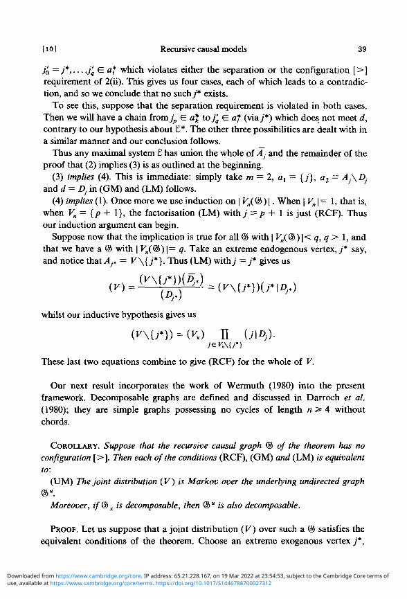
JQ=j*,...,jqGaf which violates either the separation or the configuration [>]requirement of 2(ii). This gives us four cases, each of which leads to a contradic-tion, and so we conclude that no such j * exists.

To see this, suppose that the separation requirement is violated in both cases.Then we will have a chain from jp G a£ toj^ G af (via>*) which does not meet d,contrary to our hypothesis about £*. The other three possibilities are dealt with ina similar manner and our conclusion follows.

Thus any maximal system £ has union the whole of Aj and the remainder of theproof that (2) implies (3) is as outlined at the beginning.

(3) implies (4). This is immediate: simply take m = 2, a, = {j}, a2 = AJ\DJ

and d = Dj in (GM) and (LM) follows.(4) implies (1). Once more we use induction on | Vn{%) \. When | Vn |= 1, that is,

when Vn = {p + 1}, the factorisation (LM) withy - p + 1 is just (RCF). Thusour induction argument can begin.

Suppose now that the implication is true for all ® with | Vn{%) |< q, q > 1, andthat we have a © with \Vn{%)\= q. Take an extreme endogenous vertex, j * say,and notice t h a t ^ . = K\{y*}. Thus (LM) withy =j* gives us

whilst our inductive hypothesis gives us

nThese last two equations combine to give (RCF) for the whole of V.

Our next result incorporates the work of Wermuth (1980) into the presentframework. Decomposable graphs are defined and discussed in Darroch et al.(1980); they are simple graphs possessing no cycles of length n > 4 withoutchords.

COROLLARY. Suppose that the recursive causal graph % of the theorem has noconfiguration [>]. Then each of the conditions (RCF), (GM) and (LM) is equivalentto:

(UM) The joint distribution (V) is Markov over the underlying undirected graph©".

Moreover, if®x is decomposable, then ®" is also decomposable.

PROOF. Let us suppose that a joint distribution (V) over such a © satisfies theequivalent conditions of the theorem. Choose an extreme exogenous vertex j * ,



https://doi.org/10.1017/S1446788700027312


40 Hani Kiiveri, T. P. Speed and J. B. Carlin [n]

noting once more that Aj. = V. Then for any system ax,...,am and d for which ak

and a, are separated byrf in®", l < A : < / < m , we conclude that ax,...,am aremutually conditionally independent given d under (V). But this is just theMarkov property of (F) over @".

To prove the converse we need to check that there are no additional independen-cies arising from a system a,,... ,am and d whose union is contained in AJfj notextreme. Suppose that d separates these (pairwise) in (Aj)@« but not in @". Thenthere is a chain ak 3 jo,...,jp_i,jp,jp+u.. .,jq G a, connecting some pair ak andat from the system which involves &jp$ Aj, that is, jp G Ej. Supposing, as wemay, that the chain under discussion is a minimal length one having this property,we will derive a contradiction.

Since © has no instance of configuration [>] we cannot havey^, -+jp*-jp+\,and so jp-*jp_v say, holds. Theny/,_1 -»./),_2

m u s t a l s o nold> f o r ^JP-2^JP-\then we would need to havejp_2 -*jp or jp -+jp-2 to avoid a configuration [>],but this would contradict minimality of the length of the path. This argumentcontinues down toy", ->j0. At no stage can j r , 0 «£ r «£/?, belong to Vx, for everyone of them belongs to Ej by construction. But this is just our contradiction, for

j0 G ak C Aj was part of our assumptions. Thus separation in (Aj) coincides withseparation in ©" and the first part of the corollary is proved.

The decomposability of ©" is proved by induction on | Fn(©)|. Suppose that| Vn | = 1. By assumption the graph ©" without p + 1 and its incident edgescontains no /"-cycles, r > 4. This must continue to be the case when p + 1 and itsincident edges are included, for an r-cycle, r > 4, involving p + 1 must include aconfiguration [>] with/? + 1 at its apex. The inductive step is proved in a similarway with the role of p + 1 in the foregoing taken by an extreme endogenousvertex. This completes the proof of the corollary.

EXAMPLE 2. Let Fx(©2) = {1,2,3} and Fn(©2) = (4,5), with ©2 being asdepicted in Figure 2(i) below.



https://doi.org/10.1017/S1446788700027312


1121 Recursive causal models 41

1 3

FIGURE 2(ii)

Then any joint distribution (12345) satisfying the causal Markov constraints of© 2 also satisfies those of © ", and conversely.

EXAMPLE 3. The graph Figure 3(i) below arises as part of the causal systemdescribed as two-wave two-variables, see Kiiveri and Speed (1982).

FIGURE 3(i) FIGURE 3(ii)

The associated causal factorisation is (1234) = (1)(2| 1)(3| 1)(4| 123) and thiscorresponds to the single conditional independence constraint 2 and 3 indepen-dent given 1. It is clear that there is one instance of configuration [>], involving4, and so the Markov constraint of the underlying undirected graph Figure 3(ii),namely 2 and 3 independent given 1 and 4, do not coincide with the causalMarkov constraints. To see this directly we note that Gaussian random variableswith covariance matrix 2 of the form given below satisfy the causal constraints ofFigure 3(i) but not those of Figure 3(ii).

2 =

3. Gaussian distribution

The most thoroughly studied causal systems or causal models are those inwhich the underlying distributions are Gaussian, see Joreskog (1977) and Wermuth(1980), although many people treat the subject as an aspect of regression and

44

-2-2

1

3-2

21

-1

2-2

12

-1

1

f-1-1

1

43 , 2 - ' =21

41111

31212

21122

1r224

4321



https://doi.org/10.1017/S1446788700027312


42 Hani Kiiveri, T. P. Speed and J. B. Carlin [ 13]

correlation analysis, not requiring a complete specification of the joint distribu-tion of the random variables under study, see Kang and Seneta (1980) andreferences therein. It is not hard to see that all the (conditional) independencestatements concerning our variables can be interpreted on terms of zero {partial)correlations, if we assume only that the random variables have a finite covariancematrix. The structure of 2~' in 3.1 also lends itself to deriving recursive systems oflinear equations, and it is to this topic which we now turn. A byproduct of ouranalysis is a proof of one form of the familiar path analysis rules. Generalreferences in this area include Boudon (1965), Duncan (1966, 1975), Goldbergerand Duncan (1973), Moran (1963) and Simon (1953, 1954).

Throughout this section 2 = (aAl) will denote the covariance matrix of therandom variables (X; Y), arranged in some order beginning with the p exogenous(X-) variables followed by the q endogenous (Y-) variables. The matrix 2 will bepartitioned in a way compatible with (X; Y) but we place its elements in thereverse of the usual order, that is, with au in the bottom right-hand corner. Allmean values will be taken to be zero.

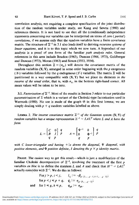
3.1. Factorisation o / 2 " ' . Most of the results in Section 3 relate to our particularparametrisation of 2 which is a variant of the Choleski-type factorisation used inWermuth (1980). No use is made of the graph @ in this first lemma; we aresimply dealing with p + q random variables labelled as above.

LEMMA 2. The inverse covariance matrix 2" 1 o/ the Gaussian system (X; Y) ofrandom variables has a unique representation 2" 1 = LALT where L and A have theform

\C 0 ] Q I"*"1 0L = [B l\ P A = [O $-'

1 P q p

with C lower-triangular and having + Is downs the diagonal, ty diagonal, withpositive elements, and 4> positive definite, I denoting the p X p identity matrix.

PROOF. The easiest way to get this result—which is just a modification of thefamiliar Choleski decomposition of 2"1 , involving the treatment of the first pvariables en bloc is to define the matrices L and A and check that H'1 = LALT

actually coincides with 2"1 . We do this as follows:

Forj>p,i<j, hj'-~ ~Pji{\ i - i i + i j - \ ) \

forp <~j^*p~^~q, \p •=z o .n — i)>

and for 1 < g, h < /> , <j>gh:= agh.



https://doi.org/10.1017/S1446788700027312


[14] " Recursive causal models 43

Here /?,•,-.fl is the partial regression coefficient of the yth variable on the ith,eliminating the variables with indices in the set a, and Ojj.a is the residual varianceof theyth variable after eliminating those with indices in a.

Writing L = (Ijj), $ = (<t>gh) and ¥ = diag(«^) (where we have added in Os andIs to the definition of L) we readily see that if H'x = LALT, then HL = L~TA'\Beginning with the bottom right-hand p X p-b\ock and continuing recursively wecan check easily from this equation that 2 = H. We omit the details.

Uniqueness is easily proved and again the details are omitted.

It is worthwhile gathering up some formulae associated with this decompositionof 2"1; they are all easily checked.

C Olf*"1 0i f IT* IT* 1

nT I I Cty~ C C^~ 8 I

Forj>p,

0 i f*<y .

The factorisation described in the preceding lemma will be called the (L; A) or(L; *, $) or (C, 5; ¥, O) decomposition of 2"1 in what follows. Notice that itdoes depend on the ordering of the random variables.

For our main result in this section we need the notion of a strict ordering of thevertices of a recursive causal graph ® compatible with the graph structure, which isan ordering <p: V -* {1,2,... ,| V\) such that

®<P(VX) = {1,2,...,| Fx |}, (u)(p(O<<Ky) whenever./E K B a n d i - j .It is not hard to see that for any recursive causal graph © there is always at

least one compatible strict ordering of V{ %).The following result concerns random variables (X; Y) indexed by the vertices

of a recursive causal graph ($ and ordered in the same way as these vertices. Theirjoint Gaussian distribution has density p%, corresponding to mean 0 and covari-ance matrix 2.

PROPOSITION 1. The distribution p% satisfies the equivalent conditions of thetheorem if and only if for all strict orderings of F(@) compatible with ©, the



https://doi.org/10.1017/S1446788700027312


44 Harri Kiiveri, T. P. Speed and J. B. Carlin [ is ]

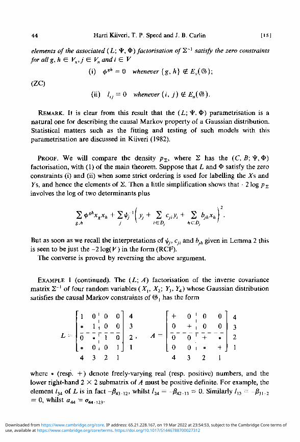
elements of the associated (L; ty, <$>) factorisation of I,'1 satisfy the zero constraintsfor all g,heVxJEVn and i £ V

(i) 4>gh = 0 whenever {g, h) <£ Ex(®);

(ZC)

(ii) lu = 0 whenever (i, j)«£„(©).

REMARK. It is clear from this result that the (L; ^ , $) parametrisation is anatural one for describing the causal Markov property of a Gaussian distribution.Statistical matters such as the fitting and testing of such models with thisparametrisation are discussed in Kiiveri (1982).

PROOF. We will compare the density />2, where 2 has the (C, B;^, $)factorisation, with (1) of the main theorem. Suppose that L and $ satisfy the zeroconstraints (i) and (ii) when some strict ordering is used for labelling the Xs andYs, and hence the elements of 2. Then a little simplification shows that -2 log p?involves the log of two determinants plus

g.h

bjhxh

But as soon as we recall the interpretations of ^ , cJi and bjh given in Lemma 2 thisis seen to be just the -2 log(F) in the form (RCF).

The converse is proved by reversing the above argument.

EXAMPLE 1 (continued). The (L; A) factorisation of the inverse covariancematrix 2"' of four random variables (A",, X2; ^3,^4) whose Gaussian distributionsatisfies the causal Markov constraints of ©, has the form

L =

1 0 ' 0 01 J 0 0

r* 1* 0 1 04 3 2

4

3

21

A =

+0

0

0

4

0+0

0

3

I

1I

1

Ii1

00

+*2

00

*

+1

4

3

2

1

where * (resp. + ) denote freely-varying real (resp. positive) numbers, and thelower right-hand 2 X 2 submatrix of A must be positive definite. For example, theelement /34 of L is in fact -/?43.12, whilst l24 — -/642.13 = 0. Similarly /13 = -/?31.2

= 0, whilst a^ = 044.123.



https://doi.org/10.1017/S1446788700027312


[161 Recursive causal models

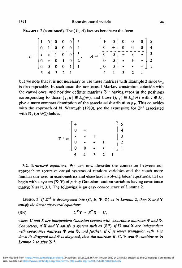
EXAMPLE 2 (continued). The (L; A) factors here have the form

45

1

0

*

0

0

0

1

*

*

0

0

0

1

0

0

00

0

1

0

0

0

0

0

1

54

3

21

A -

+0

o"0

L 05

0+

"6"0

0

4

i

ii -i

i11

i

00

+**3

00

*

+*2

00*

*+1

54

3

21

L =

5 4 3 2 1

but we note that it is not necessary to use these matrices with Example 2 since © 2

is decomposable. In such cases the non-causal Markov constraints coincide withthe causal ones, and positive definite matrices 2~' having zeros in the positionscorresponding to those {g, h) £ Ex((&), and those ( j , j) £ £„(©) with / £ Dj,give a more compact description of the associated distribution /?2 . This coincideswith the approach of N. Wermuth (1980), see the expression for 2" 1 associatedwi th®. Su

2) below.

+0*

0

0

5

+* +* * +0 * * +4 3 2 1

54

3

2

1

3.2. Structural equations. We can now describe the connexion between ourapproach to recursive causal systems of random variables and the much morefamiliar one used in econometrics and elsewhere involving linear equations. Let usbegin with a system (X; Y) of p + q Gaussian random variables having covariancematrix 2 as in 3.1. The following is an easy consequence of Lemma 2.

LEMMA 3. 7 /2" 1 is decomposed into (C, B; ¥ , $ ) as in Lemma 2, then X and Ysatisfy the linear structural equations

(SE) CT\ + Br\ = U,

where U and X are independent Gaussian vectors with covariance matrices ty and 0.Conversely, if X and Y satisfy a system such as (SE), if U and X are independentwith covariance matrices ^ and 4>, and further, if C is lower triangular with +\sdown its diagonal and ¥ is diagonal, then the matrices B, C, ¥ and 4> combine as inLemma 2 to give 2"1.



https://doi.org/10.1017/S1446788700027312


46 Hard Kiiveri, T. P. Speed and J. B. Carlin [ 17]

PROOF. This result is an immediate consequence of Lemma 2 and the formulaewhich follow it.

REMARKS, (i) It is perhaps more usual with structural equations to specify that(SE) hold with C, ty having the properties stated, and that only the conditionaldistribution of U given X be Gaussian (with mean zero and covariance matrix ty).In other words, either X is not regarded as a random vector, or it is, but noassumptions are made about its distribution. In the latter case such a specificationstill corresponds to 2" 1 having the form LALT with L and A having their usualstructure. For if CTY + BTX is normal with zero mean and covariance matrix ¥ ,given X, then Y has mean -C~TBTX and covariance matrix C'T^C'^ given X,whence Var(y) = CT*Cl + CTBTQ>BCl and Cov(7, X) = - C " r f i r $ , where$ = E(XXT) is assumed to be finite. These formulas may be compared with thosefollowing Lemma 2 and the assertion will then be evident.

A consequence of the remarks just made is the following: any conditionalindependence statements concerning (X; Y) involving A'-variables only in theconditioning which are valid when the whole system is jointly Gaussian are alsovalid if we assume only that Y given X (equivalently, U given X in the above)Gaussian.

(ii) All of the foregoing extends to the case in which only second-orderassumptions concerning U given X are made; simply replace conditional indepen-dence statements by the corresponding zero partial correlation ones.

Turning now to the Markov properties enjoyed by (X; Y) when they satisfy aset of equations such as (SE) under the further assumptions stated in Lemma 3,we have the following immediate consequence of Proposition 1.

PROPOSITION 2. A Gaussian system (X; Y) satisfying the equations (SE) with Uindependent ofX and having covariance matrices ¥ , $ respectively, C lower-triangu-lar with + ls down the diagonal and ty diagonal, also satisfies the equivalentconditions of the theorem if and only if L = (£ °t) and O satisfy the zero constraints(ZC) of Proposition 1.

In other words, we can use the theorem to draw causal graph associated withany system of structural equations such as (SE) having zeros in the lower-triangu-lar matrix C (and also in the inverse of the covariance matrix of the exogenousvariables), and then make direct conditional independence statements concerningthe endogenous variables (and also the exogenous variables) valid under thefurther assumption that Y | X [(X; Y)] is Gaussian. Once more we remark that thesame argument yield zero partial correlation statements which are generally valid.



https://doi.org/10.1017/S1446788700027312



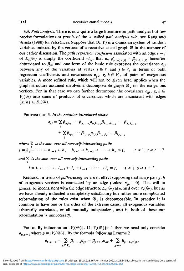
3.3. Path analysis. There is now quite a large literature on path analysis but fewprecise formulations or proofs of the so-called path analysis rule, see Kang andSeneta (1980) for references. Suppose that (X; Y) is a Gaussian system of randomvariables indexed by the vertices of a recursive causal graph © in the manner ofour earlier discussion. The path regression coefficient associated with an edge / -> jof £„(©) is simply the coefficient -lijy that is, ^ .p .^ , . ) = pJiA x ( l ) hereafterabbreviated to fijt, and one form of the basic rule expresses the covariance atJ

between any of the variables at vertex i G V and j £ Vn in terms of pathregression coefficients and covariances ogh, g, h e Vx, of pairs of exogenousvariables. A more refined rule, which will not be given here, applies when thegraph structure assumed involves a decomposable graph %x on the exogenousvertices. For in that case we can further decompose the covariance ogh, g, h GFx(@) into sums of products of covariances which are associated with edges{g, h) G Ex(®).

PROPOSITION 3. In the notation introduced above

2

where 2 is the sum over all non-self-intersecting paths

i = hx *- • • • «- hr_x «- hr - hr+x -» hr+2 -» • • • -> hu =j, r 3= 1, u > r + 2,

and 2 is the sum over all non-self-intersecting paths

/ = / , « - • • • • - / ,_, «-»,-»/ ,+ ! - • • • • -» '„ =j, s > 1, v> s + 2.

REMARK. In terms of path-tracing we are in effect supposing that every pair g, hof exogenous vertices is connected by an edge (unless ogh = 0). This will ingeneral be inconsistent with the edge structure Ex(<&) assumed over Vx(@), but aswe have already indicated a completely satisfactory but rather more complicatedreformulation of the rules exist when ©x is decomposable. In practice it iscommon to have one or the other of the extreme cases: all exogenous variablesarbitrarily correlated, or all mutually independent, and in both of these ourreformulation is unnecessary.

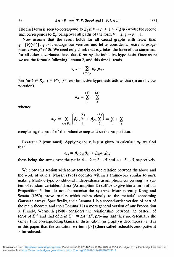
PROOF. By induction on | Vn(®)\. If | Vn(®)\— 1 then we need only considerah P+1 where/> = | Vx(<§>) \. By the formula following Lemma 2



https://doi.org/10.1017/S1446788700027312


48 Han i Kiiveri, T. P. Speed and J. B. Carlin [ 19 ]

The first term is seen to correspond to 22 if h -»p + 1 G £„(©) whilst the secondsum corresponds to 2|, being over all paths of the form h — g,g -»p + 1.

Now assume that the result holds for all causal graphs with fewer thanq —\Vn(®)\, q> 1, endogenous vertices, and let us consider an extreme exoge-nous vertex,/* of ©. We need only check that a,y, takes the form of our statement,for all other covariances have that form by the inductive hypothesis. Once morewe use the formula following Lemma 2, and this time it reads

aij*= 2 fy'iPik-

But for k £ Dj,, i e V\{j*} our inductive hypothesis tells us that (in an obviousnotation)

°,k = 2 + 21

whence

completing the proof of the inductive step and so the proposition.

EXAMPLE 2 (continued). Applying the rule just given to calculate a45 we findthat

a45 = &2a23&3 + ^43a33^53

these being the sums over the paths 4 *- 2 — 3 -> 5 and 4 «- 3 -> 5 respectively.

We close this section with some remarks on the relation between the above andthe work of others. Moran (1961) operates within a framework similar to ours,making Markov-type conditional independence assumptions concerning his sys-tem of random variables. These (Assumption II) suffice to give him a form of ourProposition 3, but do not characterise the systems. More recently Kang andSeneta (1980) prove results which relate closely to the material concerningGaussian arrays. Specifically, their Lemma 1 is a second-order version of part ofthe main theorem and their Lemma 3 is a more general version of our Proposition3. Finally, Wermuth (1980) considers the relationship between the pattern ofzeros of 2"1 and that of L in 2~' = LA~xl7, proving that they are essentially thesame iff the corresponding Gaussian distribution (or graph) is decomposable. It isin this paper that the condition we term [>] (there called reducible zero pattern)is introduced.



https://doi.org/10.1017/S1446788700027312



4. Discrete distributions

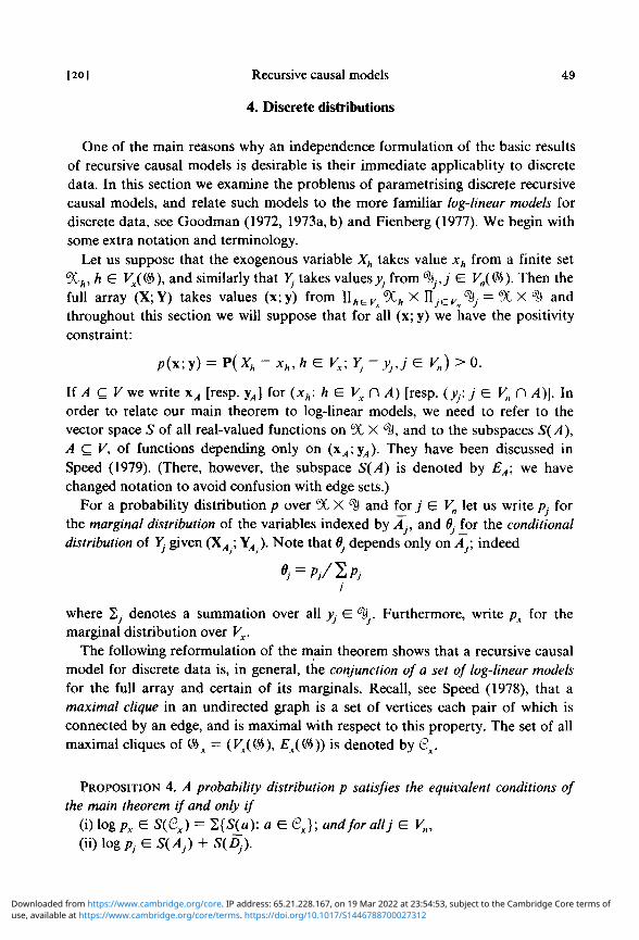
One of the main reasons why an independence formulation of the basic resultsof recursive causal models is desirable is their immediate applicablity to discretedata. In this section we examine the problems of parametrising discrete recursivecausal models, and relate such models to the more familiar log-linear models fordiscrete data, see Goodman (1972, 1973a, b) and Fienberg (1977). We begin withsome extra notation and terminology.

Let us suppose that the exogenous variable Xh takes value xh from a finite set%h,he Vx(@>), and similarly that Yj takes valuesj, from ^J G Fn(@). Then thefull array (X;Y) takes values (x;y) from Uheyx%h X RJIEyn% = % X ^ andthroughout this section we will suppose that for all (x; y) we have the positivityconstraint:

/>(x; y) = P(Xh = xh,hG Vx; Y} = Vj,j G Vn) > 0.

If A C V we write xA [resp. y j for (xh: h G Vx D A) [resp. (yy. j G Vn Pi A)]. Inorder to relate our main theorem to log-linear models, we need to refer to thevector space S of all real-valued functions on % X ty, and to the subspaces S(A),A C V, of functions depending only on (x^y^). They have been discussed inSpeed (1979). (There, however, the subspace S(A) is denoted by EA; we havechanged notation to avoid confusion with edge sets.)

For a probability distribution p over % X ^ and for j G Vn let us write D forthe marginal distribution of the variables indexed by Aj, and 0- for the conditionaldistribution of Yj given (X^ ; Y^.). Note that 0, depends only on Ay, indeed

«J = PJ/2PJj

where 1j denotes a summation over all yi G %.. Furthermore, write px for themarginal distribution over Vx.

The following reformulation of the main theorem shows that a recursive causalmodel for discrete data is, in general, the conjunction of a set of log-linear modelsfor the full array and certain of its marginals. Recall, see Speed (1978), that amaximal clique in an undirected graph is a set of vertices each pair of which isconnected by an edge, and is maximal with respect to this property. The set of allmaximal cliques of %x = (Vx(®), Ex(®)) is denoted by Qx.

PROPOSITION 4. A probability distribution p satisfies the equivalent conditions ofthe main theorem if and only if

(i) log px G S(GX) = 2{S(a): a G e,}; and for allj G Vn,



https://doi.org/10.1017/S1446788700027312


50 Harri Kiiveri, T. P. Speed and J. B. Carlin [21 ]

PROOF. These conditions are just a reformulation of (4) from the main theoremusing the Hammersley-Clifford theorem, see for example the main result of Speed(1979) for a proof in the present spirit.

Many instances of this result, with a different parametrisation, can be found inthe papers of Goodman (1972, 1973a, b; 1974a, b).

The subspace sum S(Aj) + S(Dj) may be written as

S(Aj) +[s(Dj) eS(Aj)] = S{Aj) +[S(DJ) es(Dj)],

where 0 denotes orthogonal complement in the usual inner product. This fact is aconsequence of the fact that the projections onto the various subspaces S(A) C Sall commute, and that Aj D Dj = Dj. Thus we see that if pj = exp(£y + i)j),ij e S(Aj), i\j G S(Dj)Q S(Dj), then 0, may be represented as

0, = expi j y /2 exprj7,j

and furthermore, the i\j G S(Dj) © S(Dj) is unique. Putting this into (1) of themain theorem we see that a probability p over 9C X ^ which satisfies the causalMarkov constraints has a unique representation

p =p* n T~V' whereT», e S(»J) e

S(DJ)J e vn.

Further, one can easily prove that the {r\j} are pairwise orthogonal. With prepresented in this form we see that it is possible to restrict even further thehigher-order interactions between an endogenous variable and its direct causeswithout disturbing the causal Markov constraints. Thus causal modelling withdiscrete data has two aspects: the underlying causal model, and the higher-orderinteractions just mentioned.

In closing this section we remark that when © contains no configurations [>]the causal Markov constraints collapse into a single set of log-linear constraints,those associated with what Darroch et al. (1980) call a graphical log-linear model.

5. Acknowledgements

This paper began as an honours dissertation, Carlin (1977), by one of theauthors. Its further development was greatly assisted by access to then unpub-lished work of Kang and Seneta (1980) and Wermuth (1980), and many thanksare due to these authors for their kindness. The ideas were discussed in a seminarSpeed (1978a) at the University of Copenhagen, and further thanks are due to allof the active participants in that seminar, especially Steffen Lauritzen.



https://doi.org/10.1017/S1446788700027312



Its final form is the basis for the approach adopted in a thesis, Kiiveri (1982),on causal models, and the author gratefully acknowledges the CommonwealthPostgraduate Research Scholarship held during the preparation of that thesis.

References

H. M. Blalock, Jr. (1962), 'Four-variable causal models and partial correlations', Amer. J. Sociology68, 182-194. Reprinted as Chapter 2 in Blalock (1971).

H. M. Blalock, Jr. (1971), Causal models in the social sciences (Macmillan Press Ltd., London).R. Boudon (1965), 'A method of linear causal analysis: dependence analysis', Amer. Sociological Rev.

30, 365-374.J. B. Carlin (1977), Causal models: an attempt at a unified approach (Honours thesis, Department of

Mathematics, University of Western Australia).J. N. Darroch, S. L. Lauritzen and T. P. Speed (1980), 'Log-linear models for contingency tables and

Markov fields over graphs', Ann. Statist. 8, 522-539.O. D. Duncan (1966), 'Path analysis: sociological examples', Amer. J. Sociology 72, ly 16. Reprinted as

Chapter 7 in Blalock (1971).O. D. Duncan (1975), Introduction to structural equation models (Academic Press, New York).S. E. Fienberg (1977), The analysis of cross classified categorical data (MIT Press, Cambridge,

Massachusetts).A. S. Goldberger and O. D. Duncan (1973), Structural equation models in the social sciences (Seminar

Press, New York).L. A. Goodman (1972), 'A general model for the analysis of surveys', Amer. J. Sociology 77,

1035-1086.L. A. Goodman (1973a), "The analysis of multidimensional contingency tables when some variables

are posterior to others: a modified path analysis approach', Biometrika 60, 179-192.L. A. Goodman (1973b), 'Causal analysis of data from panel studies and other kinds of surveys',

Amer.J. Sociology 78, 1135-1191.L. A. Goodman (1974a), 'Exploratory latent structure analysis using both identifiable and unidentifia-

ble models', Biometrika 61, 215-231.L. A. Goodman (1974b), 'The analysis of systems of qualitative variables when some of the variables

are unobservable, Part I—a modified latent structure approach', Amer. J. Sociology 79, 1179-1259.D. R. Heise (1975), Causal analysis (John Wiley & Sons, New York).K. G. Joreskog (1977), 'Structural equation models in the social sciences: Specification, estimation and

testing', Applications of statistics, pp. 265-287, edited by P. R. Krishnaiah (North-Holland Pub-lishing Co.).

K. M. Kang and E. Seneta (1980), 'Path analysis: an exposition', Developments in statistics 3, pp.217-246, edited by P. R. Krishnaiah (Academic Press).

H. Kiiveri (1982), A unified theory of causal models (Ph.D. thesis, in preparation).H. Kiiveri and T. P. Speed (1982), "The structural analysis of multivariate data: a review', Sociological

Methodology, to appear.P. A. P. Moran (1961), 'Path coefficients reconsidered', Austral. J. Statist. 3, 87-93.H. A. Simon (1953), 'Causal ordering and identifiability', Studies in econometric method. Chapter 3,

edited by William C. Hood and Tjalling C. Koupmans. Cowles Commission for Research inEconomics (John Wiley & Sons, New York). Reprinted in Simon (1957).

H. A. Simon (1954), 'Spurious correlation: a causal interpretation', J. Amer. Statist. Assoc. 49,467-479. Reprinted in Simon (1957).



https://doi.org/10.1017/S1446788700027312


52 Harri Kiiveri, T. P. Speed and J. B. Carlin [23]

T. P. Speed (1978), 'Relations between models for spatial data, contingency tables and Markov fieldson graphs', Proceedings of the conference on spatial patterns and processes, edited by R. L. Tweedie,Supplement to Advances in Applied Probability.

T. P. Speed (1978a), Graphical methods in the analysis of data (Lecture notes issued at the University ofCopenhagen Institute of Mathematical Statistics, 111 pp.).

T. P. Speed (1979), 'A note on nearest-neighbour Gibbs and Markov probability', Sankhya Ser. A 41,184-197.

N. Wermuth (1980), 'Linear recursive equations, covariance selection and path analysis', J. Amer.Statist. Assoc. 75, 963-972.

S. Wright (1921), 'Correlation and causation',7. Agric. Research 20, 557-585.S. Wright (1934), 'The method of path coefficients', Ann. Math. Statist. 5, 161-215.

Department of Mathematics CSIROUniversity of Western Australia Division of Mathematics and StatisticsNedlands, W.A. 6009 P.O. Box 1965, Canberra CityAustralia ACT 2601

AustraliaDepartment of Statistics1 Oxford StreetHarvard UniversityCambridge, Massachusetts 02138U.S.A.



https://doi.org/10.1017/S1446788700027312


Documents

Recursive causal models