Recursive Bayes Filtering

Advanced AI

Wolfram Burgard

Tutorial Goal

To familiarize you with probabilistic paradigm in robotics

! Basic techniques• Advantages• Pitfalls and limitations

! Successful Applications! Open research issues

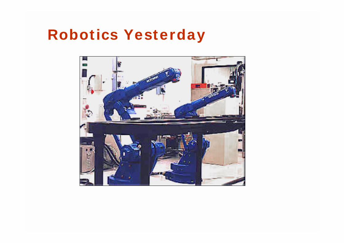
Robotics Yesterday

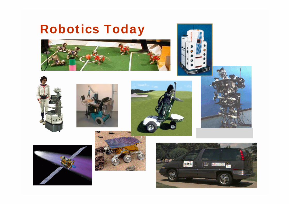
Robotics Today

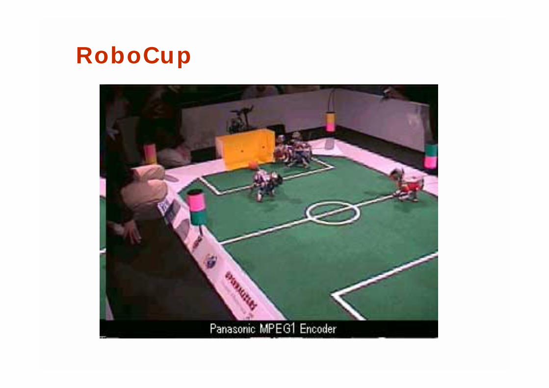
RoboCup

Physical Agents are Inherently Uncertain

! Uncertainty arises from four major factors:! Environment stochastic, unpredictable! Robot stochastic! Sensor limited, noisy! Models inaccurate

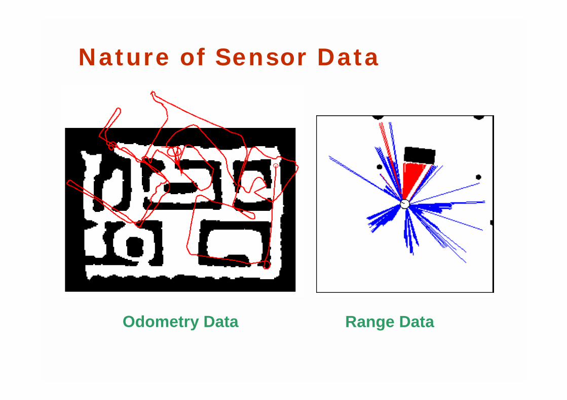
Nature of Sensor Data

Odometry Data Range Data

Probabilistic Techniques for Physical Agents

Key idea: Explicit representation of uncertainty using the calculus of probability theory

Perception = state estimationAction = utility optimization

Advantages of Probabilistic Paradigm

! Can accommodate inaccurate models! Can accommodate imperfect sensors! Robust in real-world applications! Best known approach to many hard

robotics problems

Pitfalls

! Computationally demanding! False assumptions! Approximate

Outline

! Introduction! Probabilistic State Estimation! Robot Localization! Probabilistic Decision Making

! Planning! Between MDPs and POMDPs! Exploration

! Conclusions

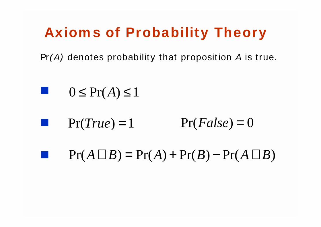
Pr(A) denotes probability that proposition A is true.

!

!

!

Axioms of Probability Theory

1)Pr(0 ≤≤ A

1)Pr( =True

)Pr()Pr()Pr()Pr( BABABA ∧−+=∨

0)Pr( =False

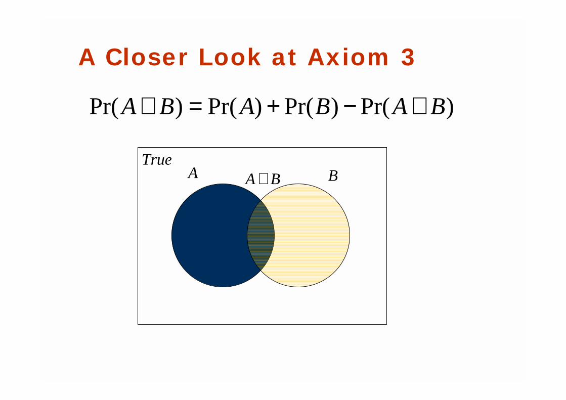
A Closer Look at Axiom 3

B

BA ∧A BTrue

)Pr()Pr()Pr()Pr( BABABA ∧−+=∨

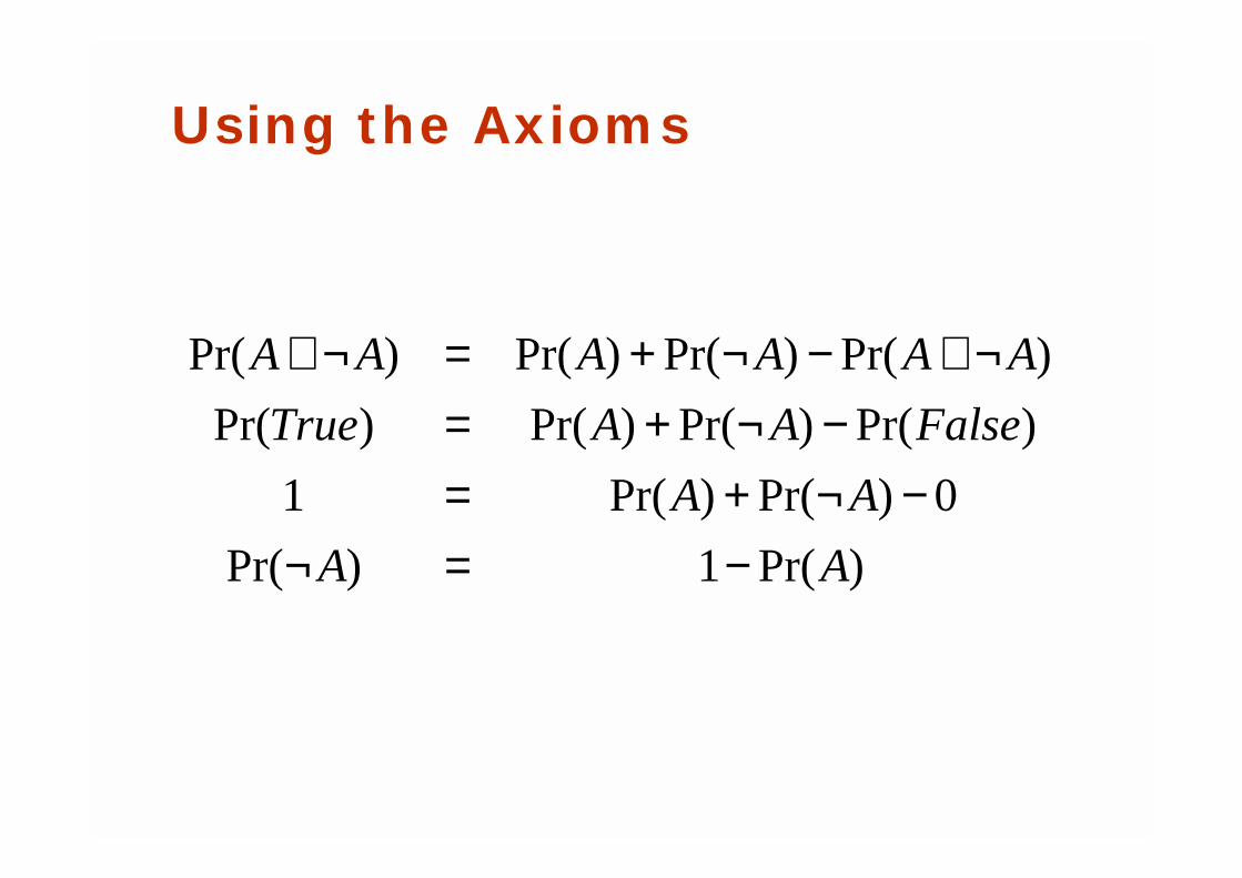
Using the Axioms

)Pr(1)Pr(

0)Pr()Pr(1

)Pr()Pr()Pr()Pr(

)Pr()Pr()Pr()Pr(

AA

AA

FalseAATrue

AAAAAA

−=¬−¬+=

−¬+=¬∧−¬+=¬∨

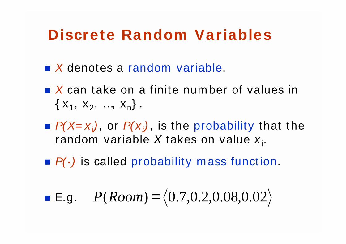
Discrete Random Variables

! X denotes a random variable.

! X can take on a finite number of values in {x1, x2, …, xn}.

! P(X=xi), or P(xi), is the probability that the random variable X takes on value xi.

! P( ) is called probability mass function.

! E.g. 02.0,08.0,2.0,7.0)( =RoomP

.

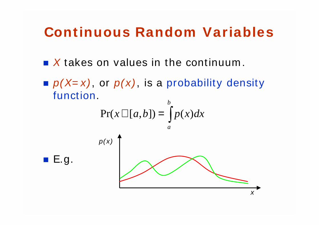
Continuous Random Variables

! X takes on values in the continuum.

! p(X=x), or p(x), is a probability density function.

! E.g.

∫=∈b

a

dxxpbax )(]),[Pr(

x

p(x)

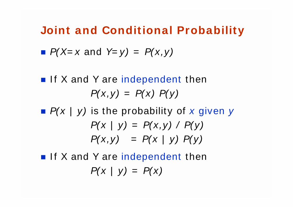
Joint and Conditional Probability

! P(X=x and Y=y) = P(x,y)

! If X and Y are independent then P(x,y) = P(x) P(y)

! P(x | y) is the probability of x given yP(x | y) = P(x,y) / P(y)P(x,y) = P(x | y) P(y)

! If X and Y are independent thenP(x | y) = P(x)

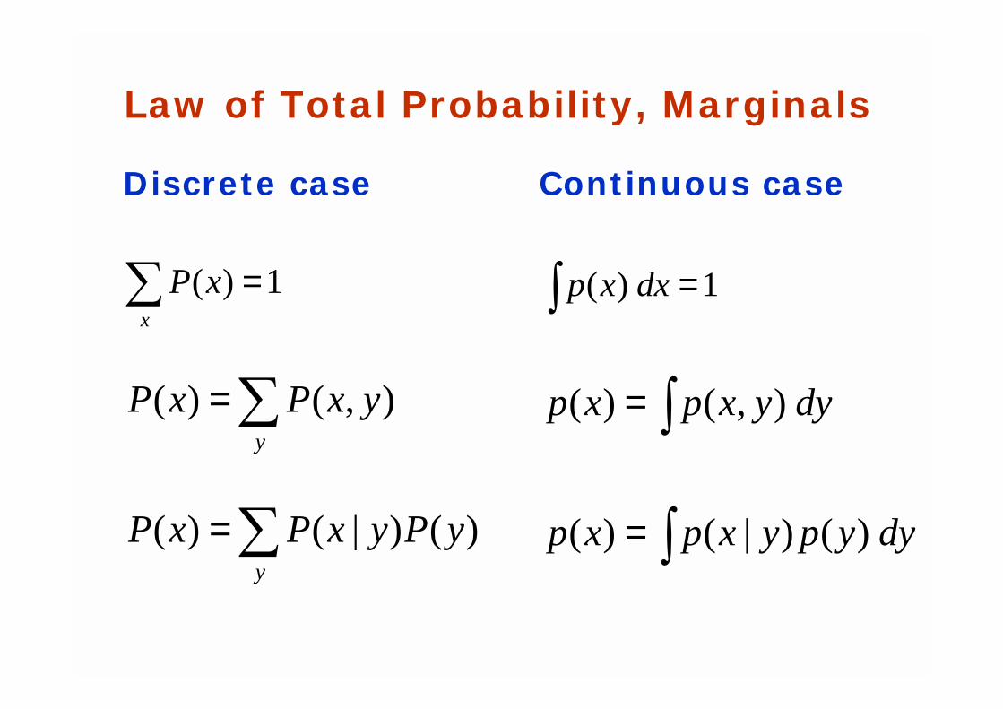
Law of Total Probability, Marginals

∑=y

yxPxP ),()(

∑=y

yPyxPxP )()|()(

∑ =x

xP 1)(

Discrete case

∫ =1)( dxxp

Continuous case

∫= dyypyxpxp )()|()(

∫= dyyxpxp ),()(

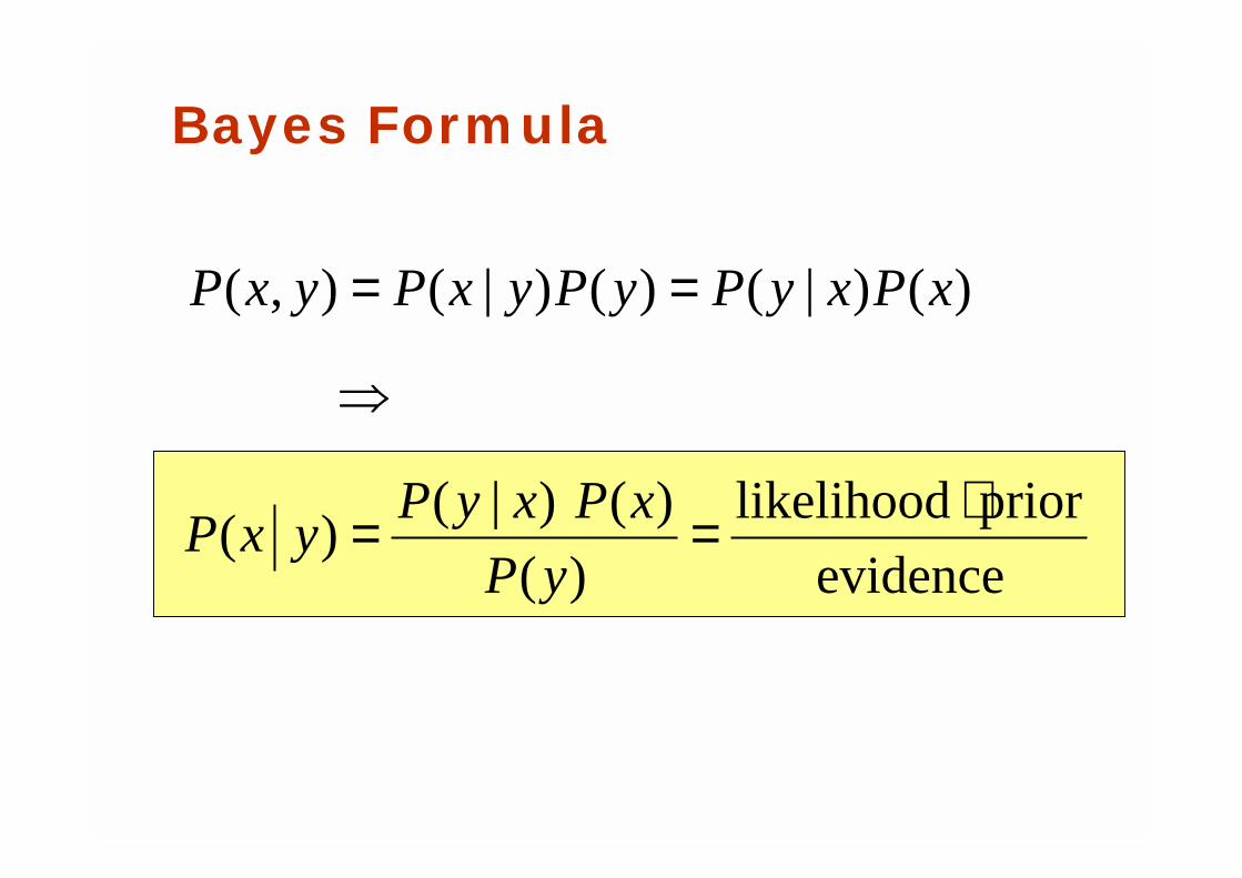
Bayes Formula

evidence

prior likelihood

)(

)()|()(

)()|()()|(),(

⋅==

⇒

==

yP

xPxyPyxP

xPxyPyPyxPyxP

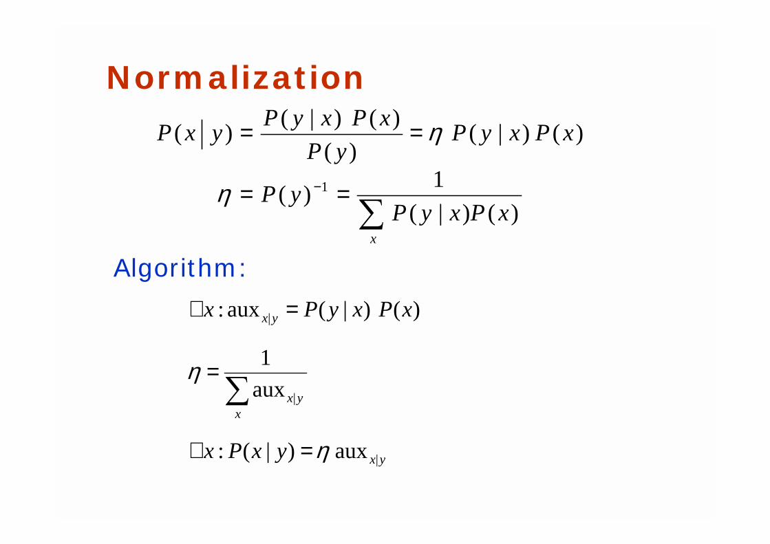
Normalization

)()|(

1)(

)()|()(

)()|()(

1

xPxyPyP

xPxyPyP

xPxyPyxP

x∑

==

==

−η

η

yx

xyx

yx

yxPx

xPxyPx

|

|

|

aux)|(:

aux

1

)()|(aux:

η

η

=∀

=

=∀

∑

Algorithm:

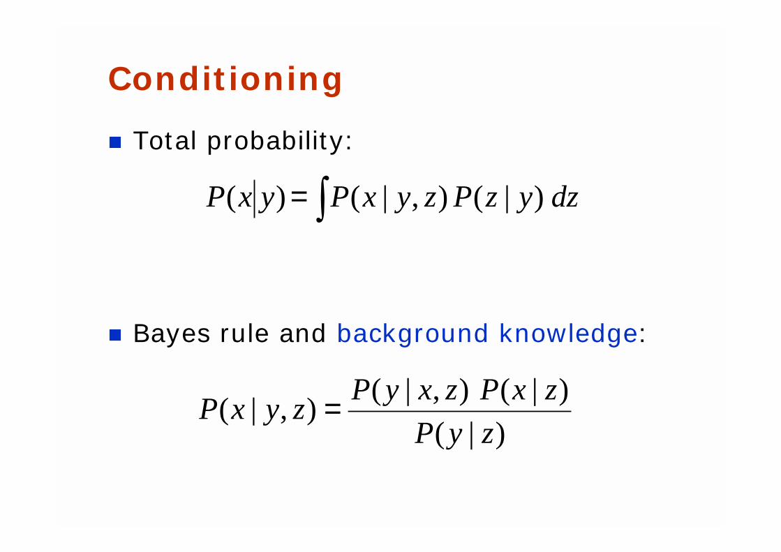
Conditioning

! Total probability:

! Bayes rule and background knowledge:

)|(

)|(),|(),|(

zyP

zxPzxyPzyxP =

∫= dzyzPzyxPyxP )|(),|()(

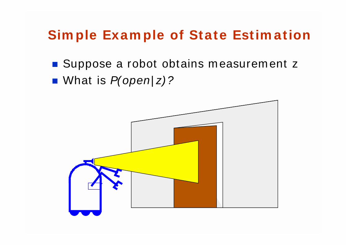
Simple Example of State Estimation

! Suppose a robot obtains measurement z! What is P(open|z)?

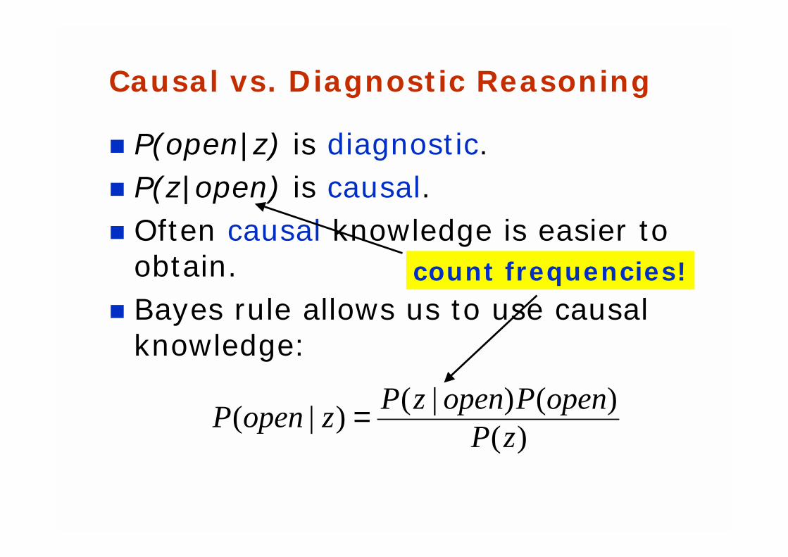
Causal vs. Diagnostic Reasoning

! P(open|z) is diagnostic.! P(z|open) is causal.! Often causal knowledge is easier to

obtain.! Bayes rule allows us to use causal

knowledge:

)()()|(

)|(zP

openPopenzPzopenP =

count frequencies!

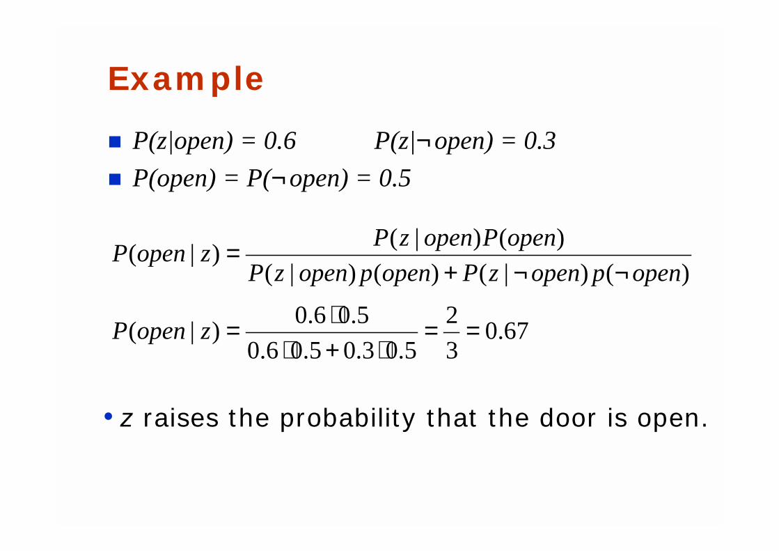
Example

! P(z|open) = 0.6 P(z|¬open) = 0.3

! P(open) = P(¬open) = 0.5

67.03

2

5.03.05.06.0

5.06.0)|(

)()|()()|(

)()|()|(

==⋅+⋅

⋅=

¬¬+=

zopenP

openpopenzPopenpopenzP

openPopenzPzopenP

• z raises the probability that the door is open.

Combining Evidence

! Suppose our robot obtains another observation z2.

! How can we integrate this new information?

! More generally, how can we estimateP(x| z1...zn )?

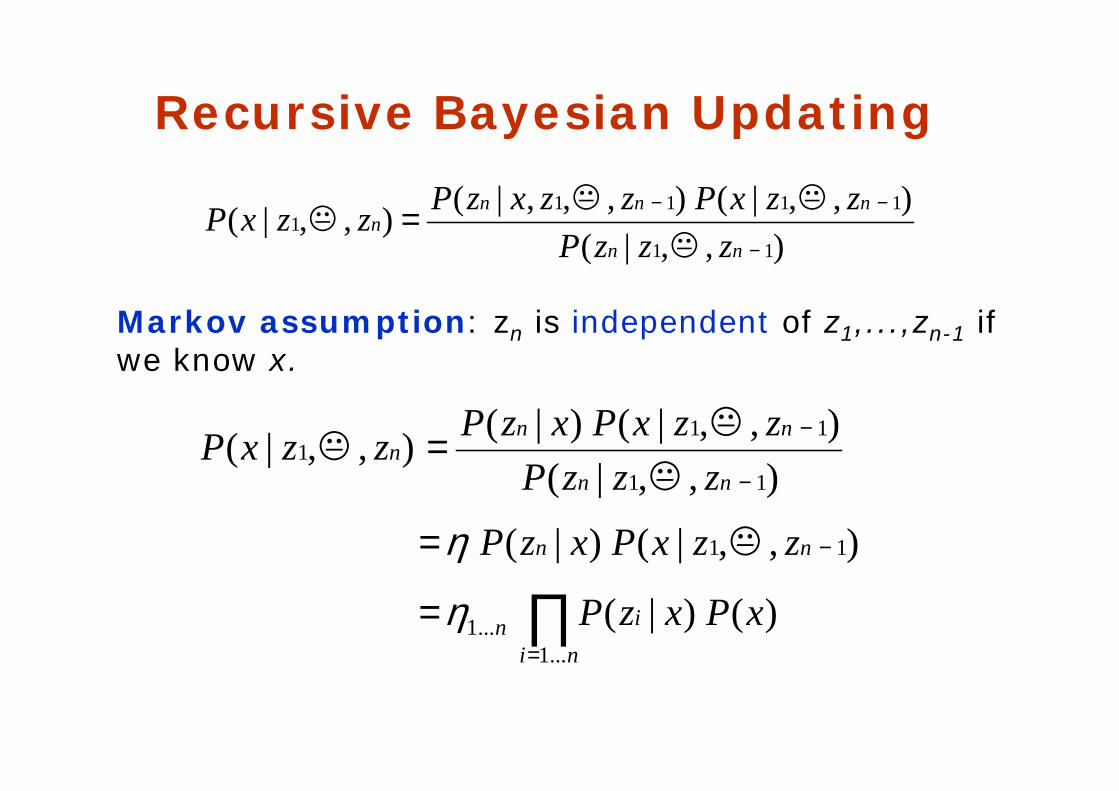
Recursive Bayesian Updating

),,|(

),,|(),,,|(),,|(

11

11111

−

−−=nn

nnnn

zzzP

zzxPzzxzPzzxP

"

"""

Markov assumption: zn is independent of z1,...,zn-1 if we know x.

)()|(

),,|()|(

),,|(

),,|()|(),,|(

...1...1

11

11

111

xPxzP

zzxPxzP

zzzP

zzxPxzPzzxP

ni

in

nn

nn

nnn

∏=

−

−

−

=

=

=

η

η "

"

""

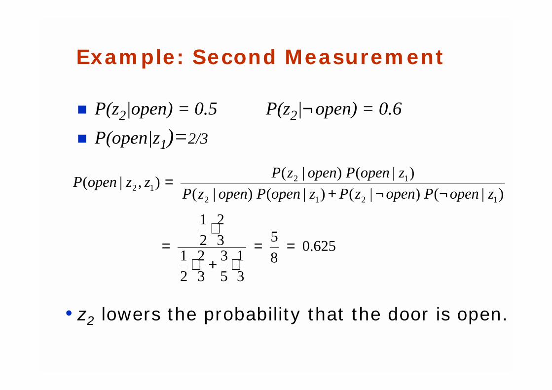
Example: Second Measurement

! P(z2|open) = 0.5 P(z2|¬open) = 0.6

! P(open|z1)=2/3

625.08

5

31

53

32

21

32

21

)|()|()|()|(

)|()|(),|(

1212

1212

==⋅+⋅

⋅=

¬¬+=

zopenPopenzPzopenPopenzP

zopenPopenzPzzopenP

• z2 lowers the probability that the door is open.

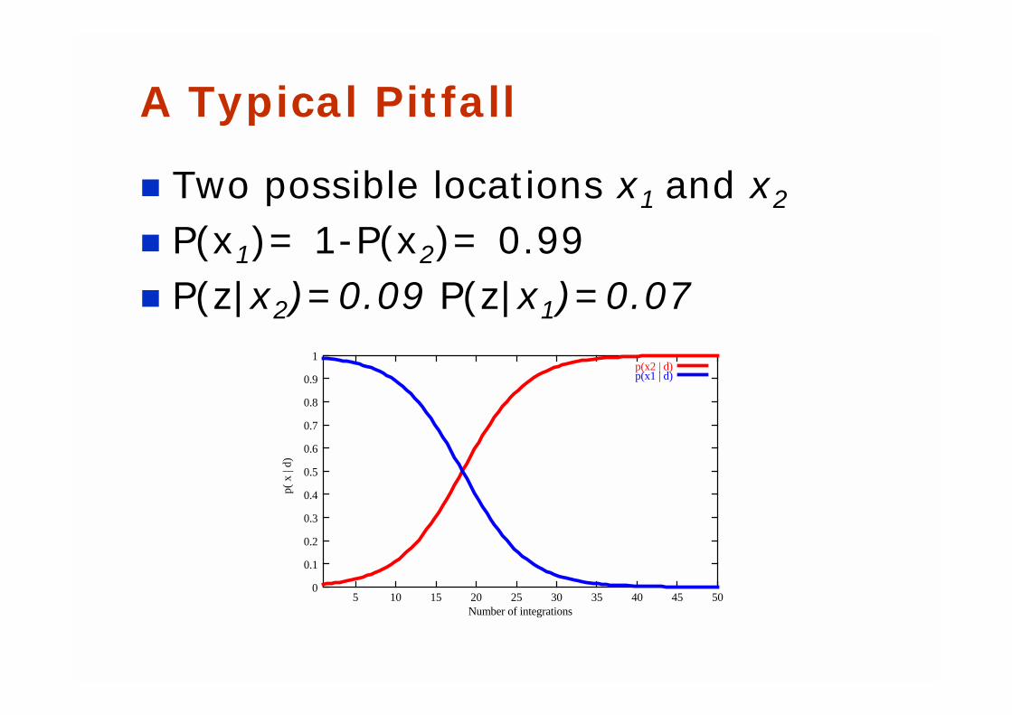
A Typical Pitfall

! Two possible locations x1 and x2

! P(x1)= 1-P(x2)= 0.99 ! P(z|x2)=0.09 P(z|x1)=0.07

0

0.1

0.2

0.3

0.4

0.5

0.6

0.7

0.8

0.9

1

5 10 15 20 25 30 35 40 45 50

p( x

| d)

Number of integrations

p(x2 | d)p(x1 | d)

Actions

! Often the world is dynamic since! actions carried out by the robot,! actions carried out by other agents,! or just the time passing by

change the world.

! How can we incorporate such actions?

Typical Actions

! The robot turns its wheels to move! The robot uses its manipulator to grasp

an object! Plants grow over time…

! Actions are never carried out with absolute certainty.

! In contrast to measurements, actions generally increase the uncertainty.

Modeling Actions

! To incorporate the outcome of an action u into the current “belief”, we use the conditional pdf

P(x|u,x’)

! This term specifies the pdf that executing u changes the state from x’ to x.

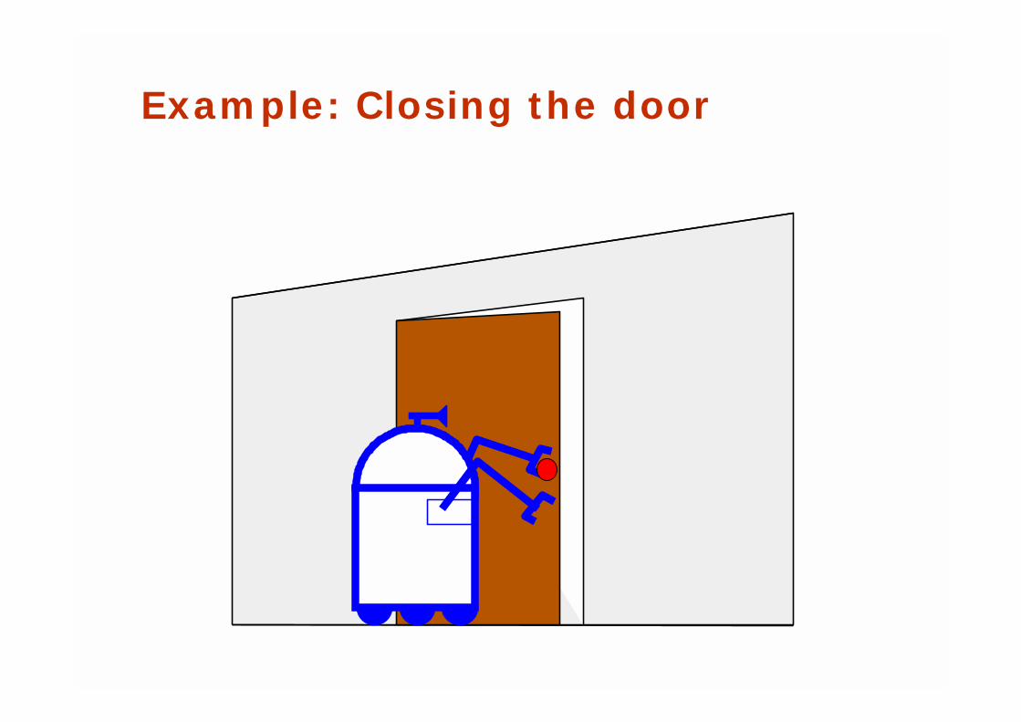
Example: Closing the door

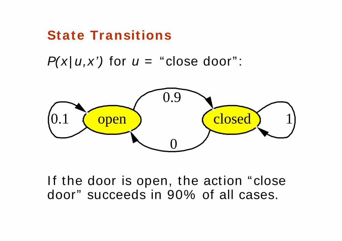
State Transitions

P(x|u,x’) for u = “close door”:

If the door is open, the action “close door” succeeds in 90% of all cases.

open closed0.1 1

0.9

0

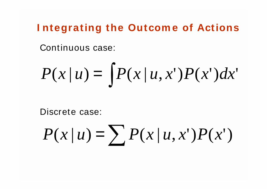
Integrating the Outcome of Actions

∫= ')'()',|()|( dxxPxuxPuxP

∑= )'()',|()|( xPxuxPuxP

Continuous case:

Discrete case:

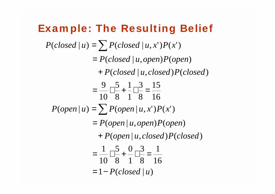
Example: The Resulting Belief

)|(1161

83

10

85

101

)(),|(

)(),|(

)'()',|()|(1615

83

11

85

109

)(),|(

)(),|(

)'()',|()|(

uclosedP

closedPcloseduopenP

openPopenuopenP

xPxuopenPuopenP

closedPcloseduclosedP

openPopenuclosedP

xPxuclosedPuclosedP

−=

=∗+∗=

+=

=

=∗+∗=

+=

=

∑

∑

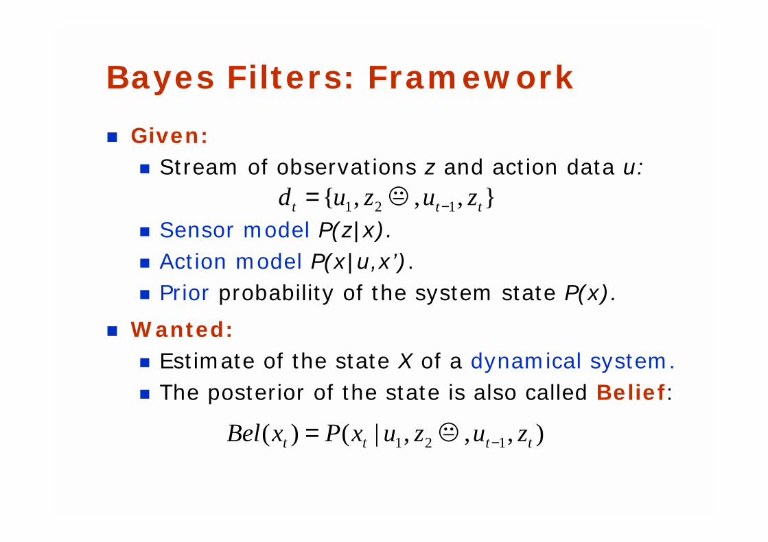
Bayes Filters: Framework

! Given:! Stream of observations z and action data u:

! Sensor model P(z|x).! Action model P(x|u,x’).! Prior probability of the system state P(x).

! Wanted: ! Estimate of the state X of a dynamical system.! The posterior of the state is also called Belief:

),,,|()( 121 tttt zuzuxPxBel −= "

},,,{ 121 ttt zuzud −= "

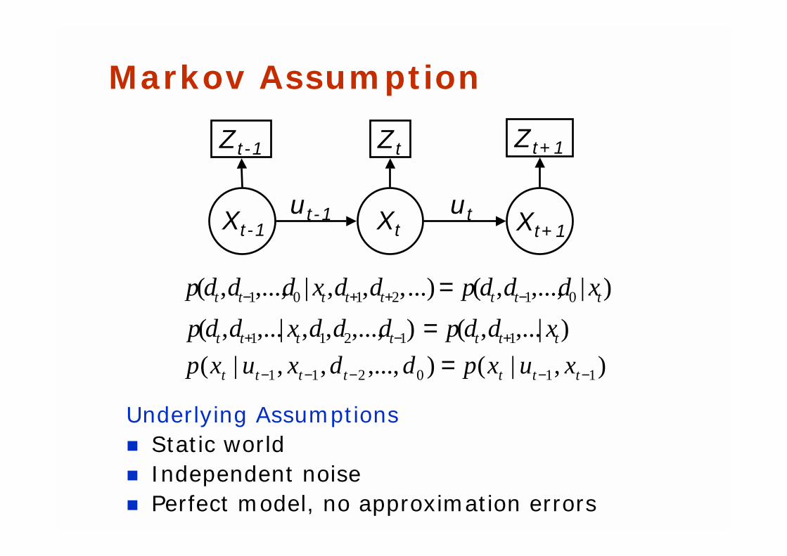
Markov Assumption

Underlying Assumptions! Static world! Independent noise! Perfect model, no approximation errors

)|,...,(),...,,,|,...,( 11211 ttttttt xddpdddxddp +−+ =)|,...,,(...),,,|,...,,( 012101 tttttttt xdddpddxdddp −++− =

Xt-1 Xt Xt+1

Zt-1 Zt Zt+1

ut-1 ut

),|(),...,,,|( 110211 −−−−− = ttttttt xuxpddxuxp

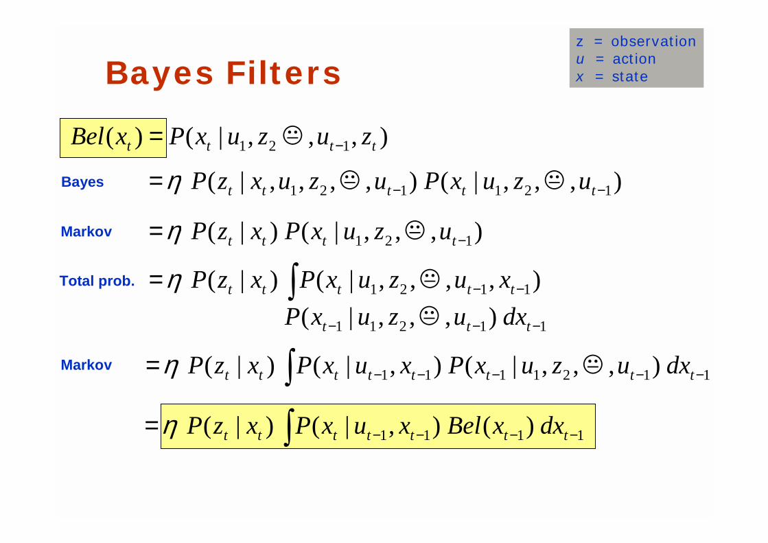
Bayes Filters

),,,|(),,,,|( 121121 −−= ttttt uzuxPuzuxzP ""ηBayes

z = observationu = actionx = state

),,,|()( 121 tttt zuzuxPxBel −= "

Markov ),,,|()|( 121 −= tttt uzuxPxzP "η

1111 )(),|()|( −−−−∫= ttttttt dxxBelxuxPxzPη

Markov1121111 ),,,|(),|()|( −−−−−∫= tttttttt dxuzuxPxuxPxzP "η

11211

1121

),,,|(

),,,,|()|(

−−−

−−∫=

ttt

ttttt

dxuzuxP

xuzuxPxzP

"

"ηTotal prob.

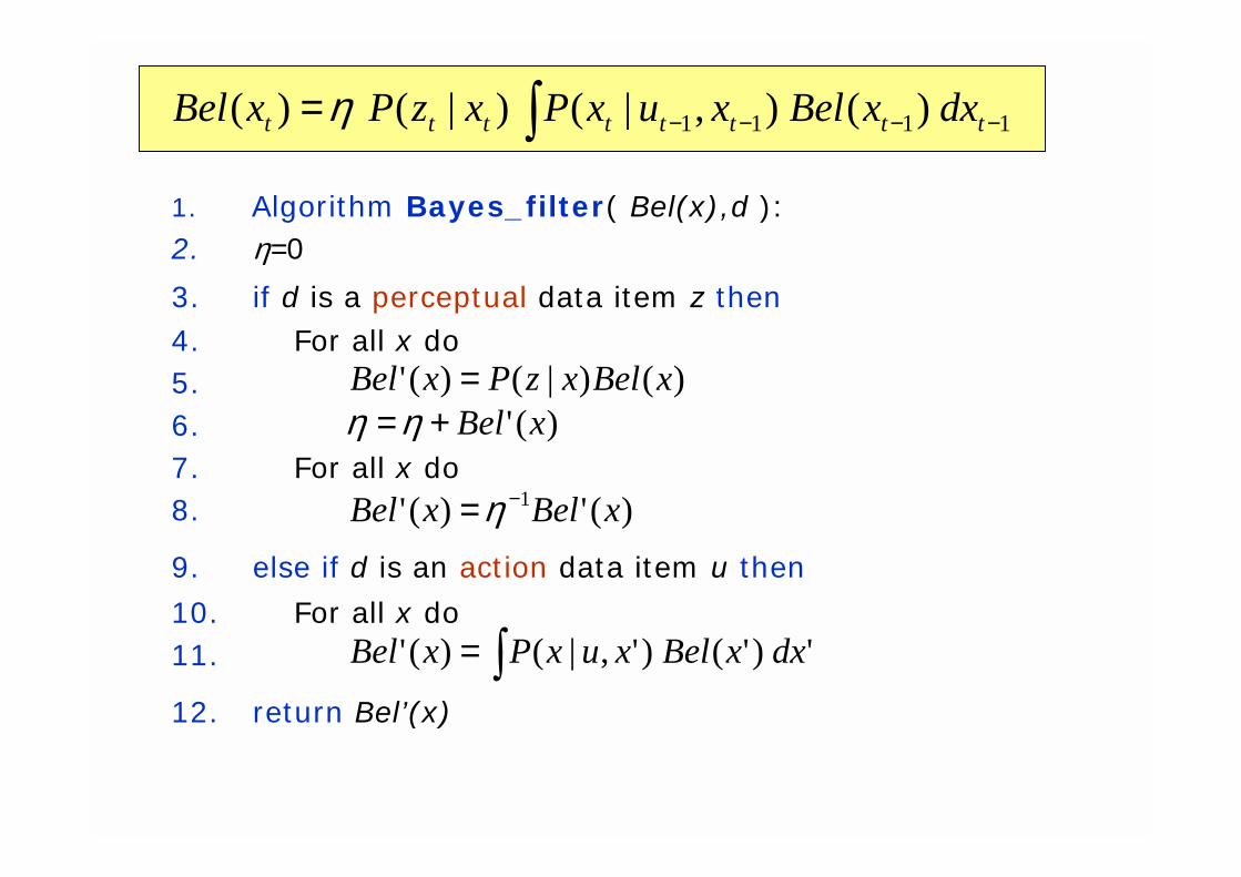
Bayes Filter Algorithm

1. Algorithm Bayes_filter( Bel(x),d ):2. η=0

3. if d is a perceptual data item z then4. For all x do5.6.7. For all x do8.

9. else if d is an action data item u then

10. For all x do11.

12. return Bel’(x)

)()|()(' xBelxzPxBel =)(' xBel+=ηη

)(')(' 1 xBelxBel −=η

')'()',|()(' dxxBelxuxPxBel ∫=

1111 )(),|()|()( −−−−∫= tttttttt dxxBelxuxPxzPxBel η

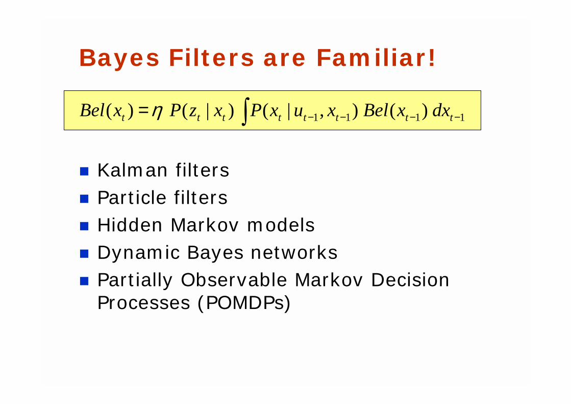
Bayes Filters are Familiar!

! Kalman filters! Particle filters! Hidden Markov models! Dynamic Bayes networks! Partially Observable Markov Decision

Processes (POMDPs)

1111 )(),|()|()( −−−−∫= tttttttt dxxBelxuxPxzPxBel η

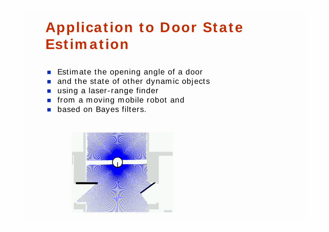
Application to Door State Estimation

! Estimate the opening angle of a door! and the state of other dynamic objects! using a laser-range finder! from a moving mobile robot and! based on Bayes filters.

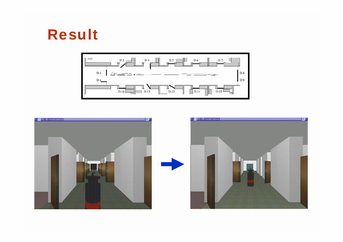
Result

Lessons Learned

! Bayes rule allows us to compute probabilities that are hard to assess otherwise.

! Under the Markov assumption, recursive Bayesian updating can be used to efficiently combine evidence.

! Bayes filters are a probabilistic tool for estimating the state of dynamic systems.

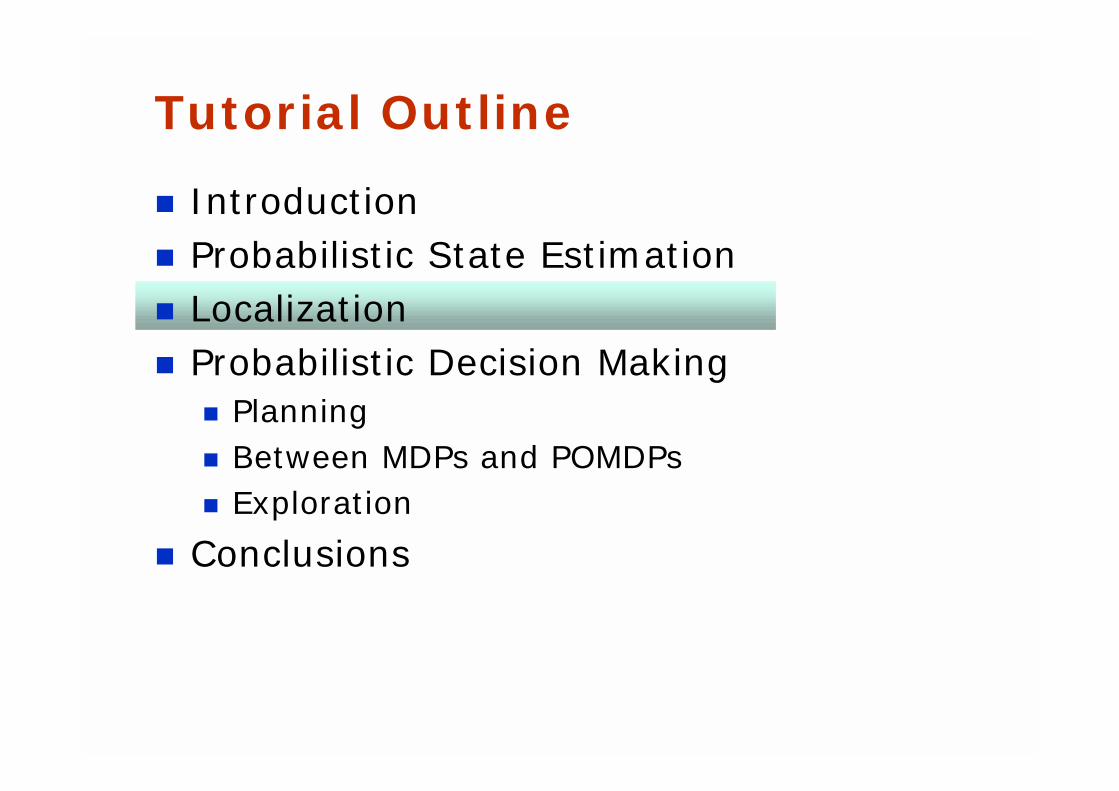
Tutorial Outline

! Introduction! Probabilistic State Estimation! Localization! Probabilistic Decision Making

! Planning! Between MDPs and POMDPs! Exploration

! Conclusions

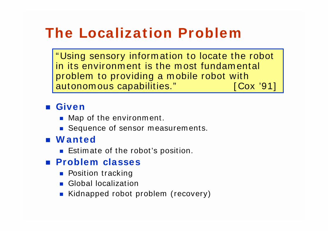
The Localization Problem

! Given! Map of the environment.! Sequence of sensor measurements.

! Wanted! Estimate of the robot’s position.

! Problem classes! Position tracking! Global localization! Kidnapped robot problem (recovery)

“Using sensory information to locate the robot in its environment is the most fundamental problem to providing a mobile robot with autonomous capabilities.” [Cox ’91]

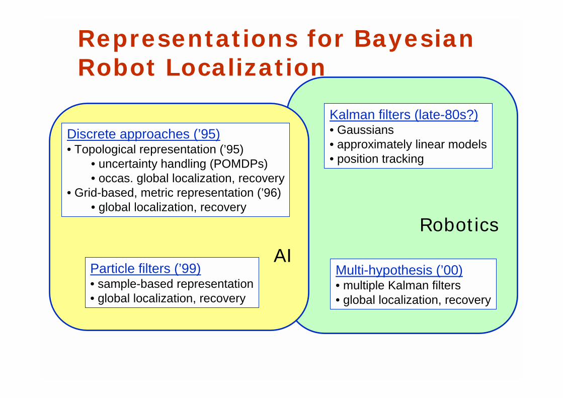
Representations for Bayesian Robot Localization

Discrete approaches (’95)• Topological representation (’95)

• uncertainty handling (POMDPs)• occas. global localization, recovery

• Grid-based, metric representation (’96)• global localization, recovery

Multi-hypothesis (’00)• multiple Kalman filters• global localization, recovery

Particle filters (’99)• sample-based representation• global localization, recovery

Kalman filters (late-80s?)• Gaussians• approximately linear models• position tracking

AI

Robotics

What is the Right Representation?

! Kalman filters

! Multi-hypothesis tracking

! Grid-based representations

! Topological approaches

! Particle filters

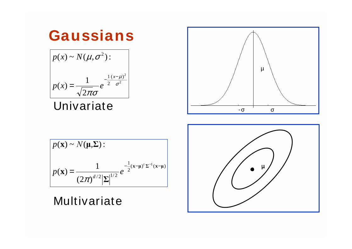
Gaussians

2

2)(

2

1

2

2

1)(

:),(~)(

σµ

σπ

σµ

−−=

x

exp

Nxp

-σ σ

µ

Univariate

)()(2

1

2/12/

1

)2(

1)(

:)(~)(

µxΣµx

Σx

Σµx

−−− −

=t

ep

,Νp

dπµµµµ

Multivariate

49

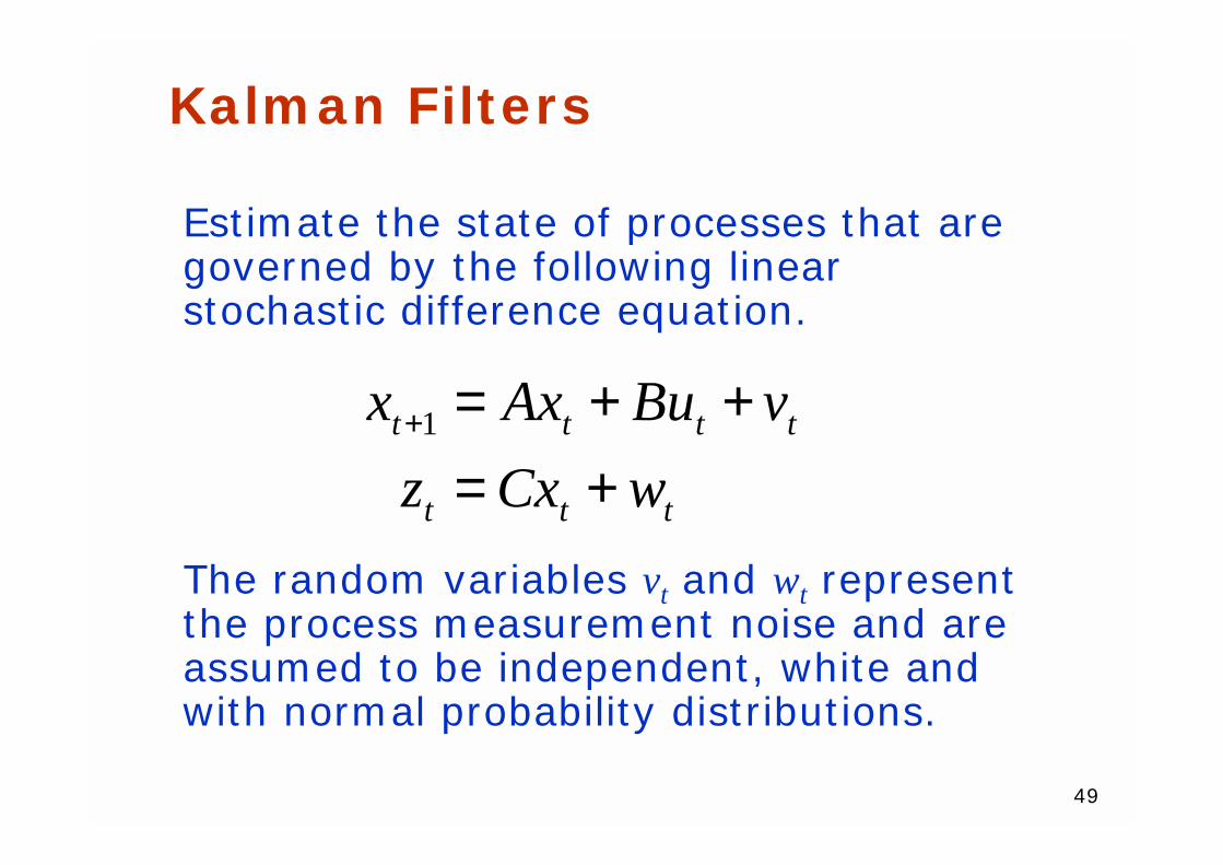
Kalman Filters

Estimate the state of processes that are governed by the following linear stochastic difference equation.

The random variables vt and wt represent the process measurement noise and are assumed to be independent, white and with normal probability distributions.

ttt

tttt

wCxz

vBuAxx

+=++=+1

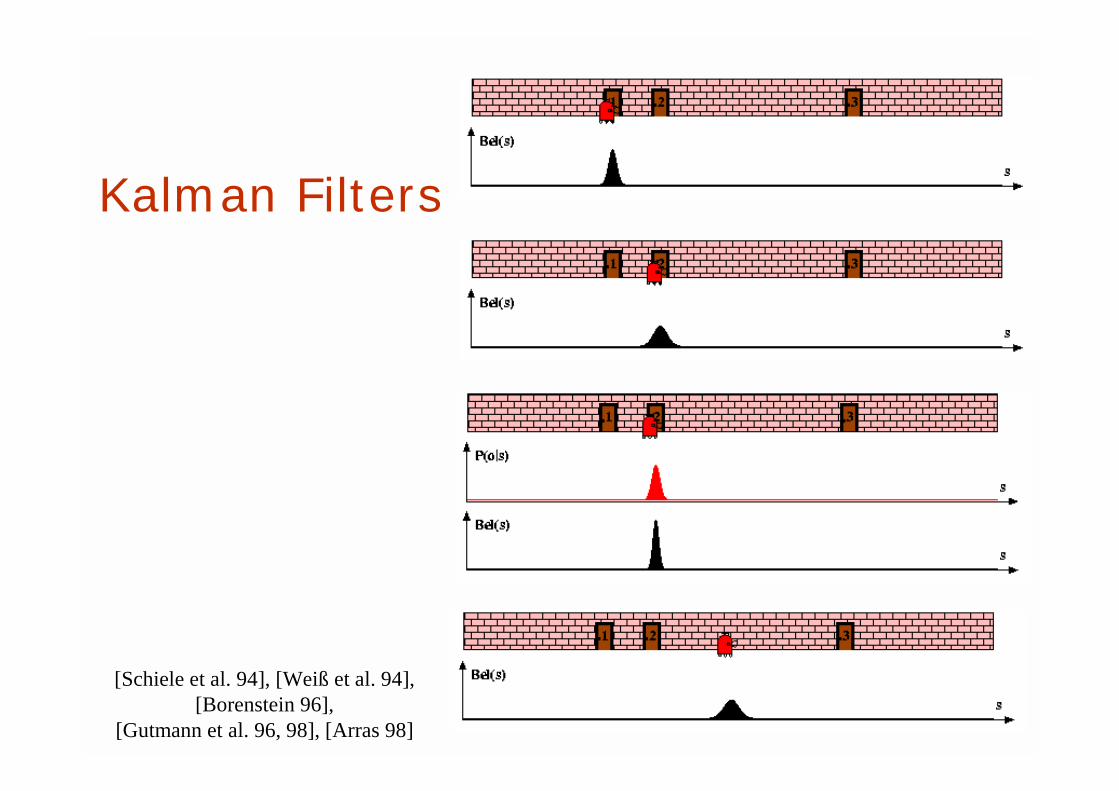
[Schiele et al. 94], [Weiß et al. 94], [Borenstein 96],

[Gutmann et al. 96, 98], [Arras 98]

Kalman Filters

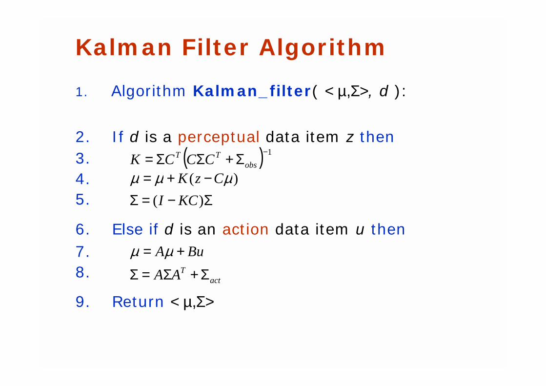
Kalman Filter Algorithm

1. Algorithm Kalman_filter( <µ,Σ>, d ):

2. If d is a perceptual data item z then3.4.5.

6. Else if d is an action data item u then7.8.

9. Return <µ,Σ>

Σ−=Σ )( KCI

( ) 1−Σ+ΣΣ= obsTT CCCK

)( µµµ CzK −+=

actTAA Σ+Σ=ΣBuA += µµ

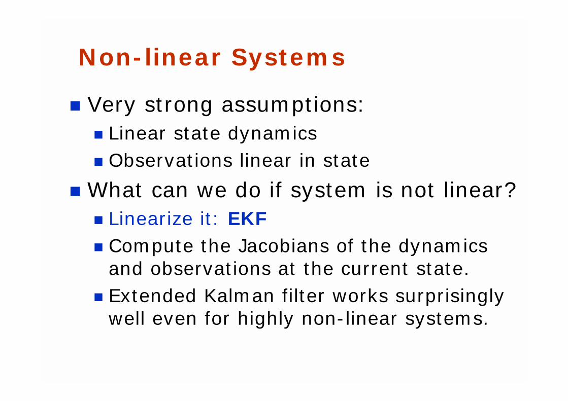
Non-linear Systems

! Very strong assumptions:! Linear state dynamics! Observations linear in state

! What can we do if system is not linear?! Linearize it: EKF! Compute the Jacobians of the dynamics

and observations at the current state.! Extended Kalman filter works surprisingly

well even for highly non-linear systems.

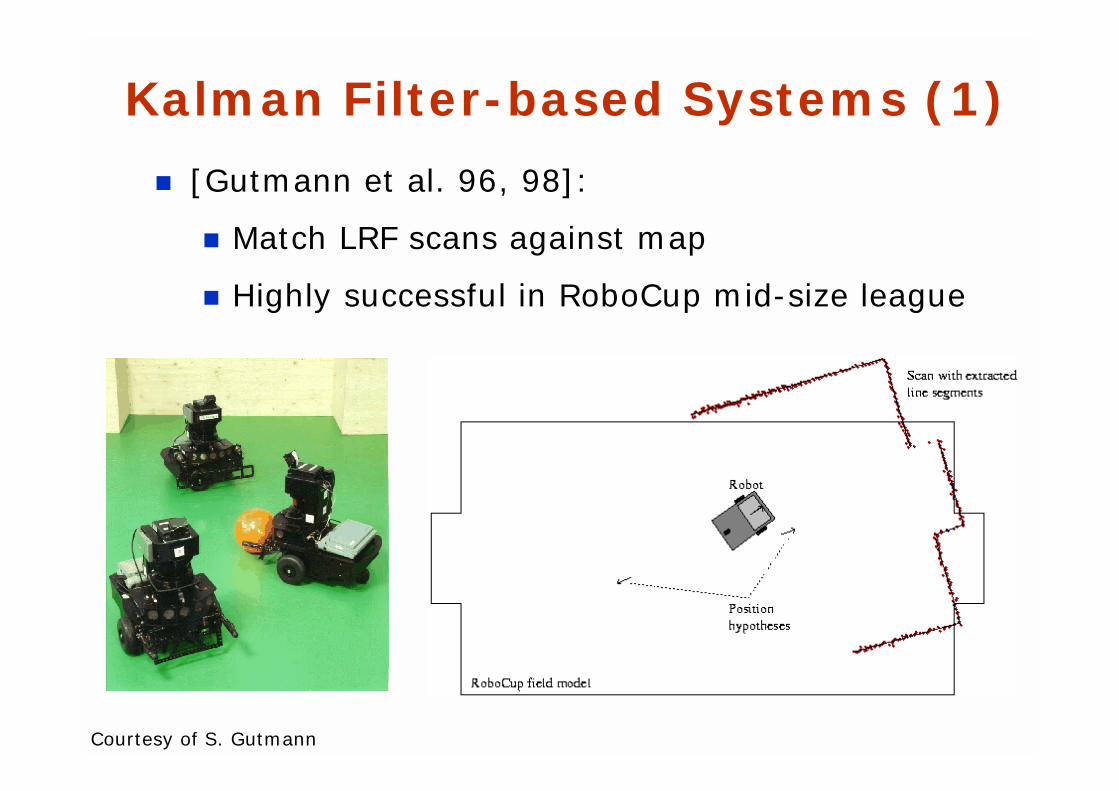
! [Gutmann et al. 96, 98]:

! Match LRF scans against map

! Highly successful in RoboCup mid-size league

Kalman Filter-based Systems (1)

Courtesy of S. Gutmann

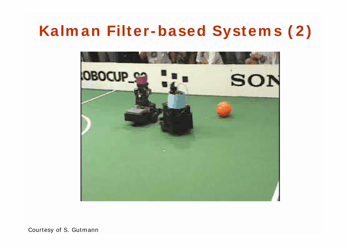
Kalman Filter-based Systems (2)

Courtesy of S. Gutmann

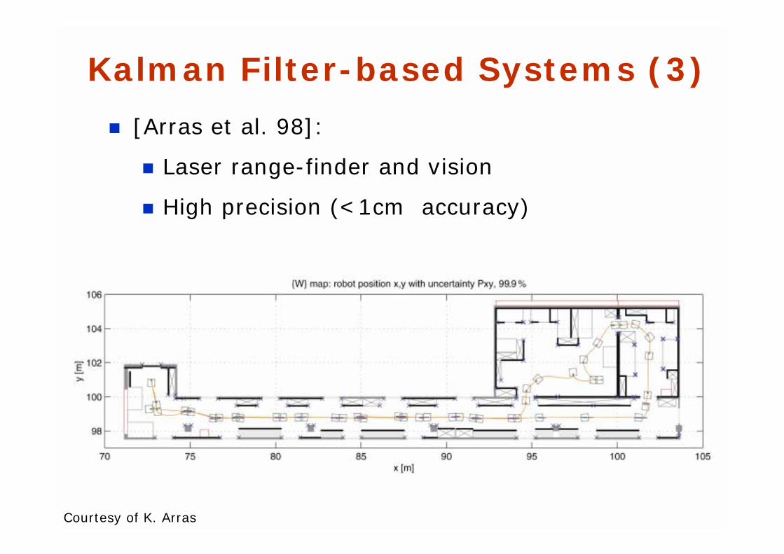
! [Arras et al. 98]:

! Laser range-finder and vision

! High precision (<1cm accuracy)

Kalman Filter-based Systems (3)

Courtesy of K. Arras

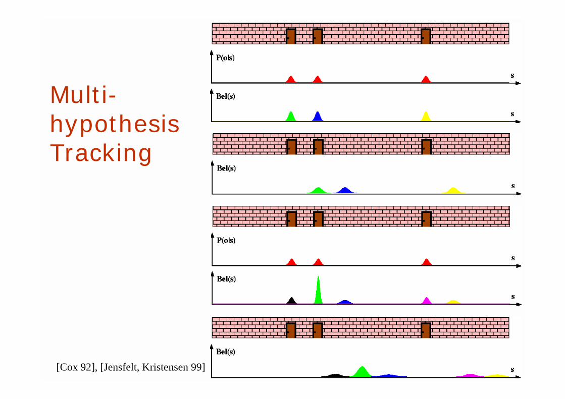
[Cox 92], [Jensfelt, Kristensen 99]

Multi-hypothesisTracking

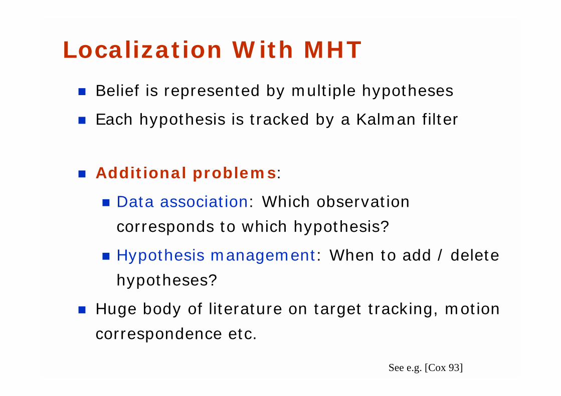
! Belief is represented by multiple hypotheses

! Each hypothesis is tracked by a Kalman filter

! Additional problems:

! Data association: Which observation

corresponds to which hypothesis?

! Hypothesis management: When to add / delete

hypotheses?

! Huge body of literature on target tracking, motion

correspondence etc.

Localization With MHT

See e.g. [Cox 93]

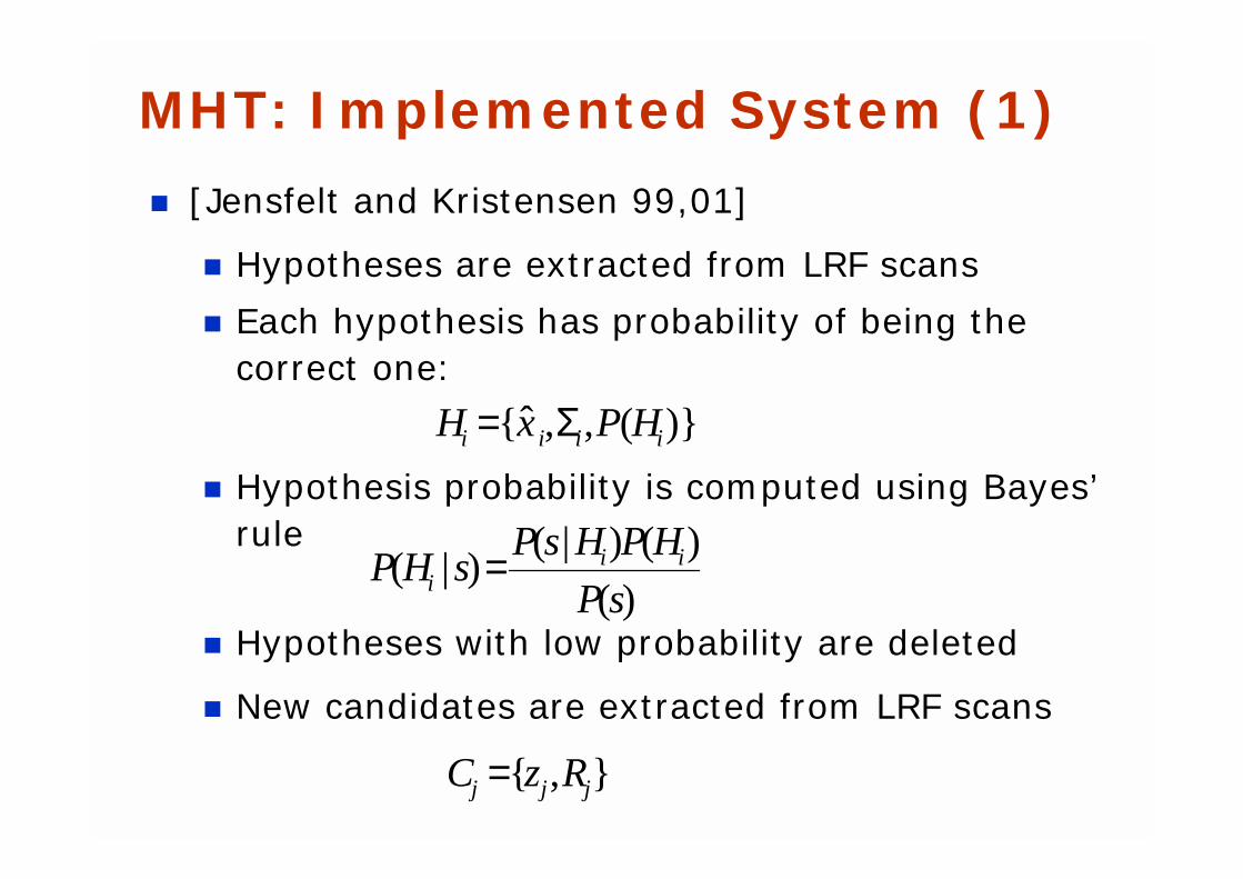
! [Jensfelt and Kristensen 99,01]

! Hypotheses are extracted from LRF scans

! Each hypothesis has probability of being the correct one:

! Hypothesis probability is computed using Bayes’ rule

! Hypotheses with low probability are deleted

! New candidates are extracted from LRF scans

MHT: Implemented System (1)

)}(,,ˆ{ iiii HPxH Σ=

},{ jjj RzC =

)(

)()|()|(

sP

HPHsPsHP ii

i =

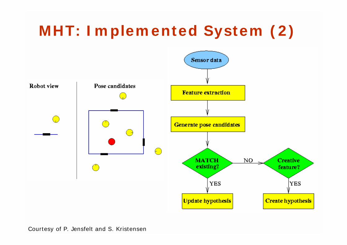
MHT: Implemented System (2)

Courtesy of P. Jensfelt and S. Kristensen

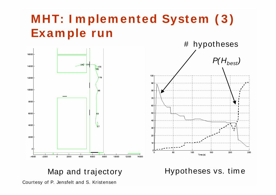
MHT: Implemented System (3)Example run

Map and trajectory

# hypotheses

Hypotheses vs. time

P(Hbest)

Courtesy of P. Jensfelt and S. Kristensen

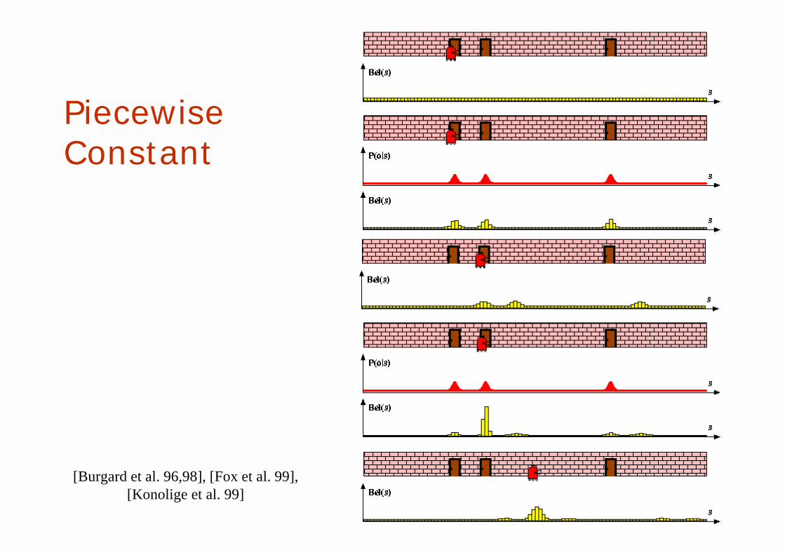
[Burgard et al. 96,98], [Fox et al. 99], [Konolige et al. 99]

Piecewise Constant

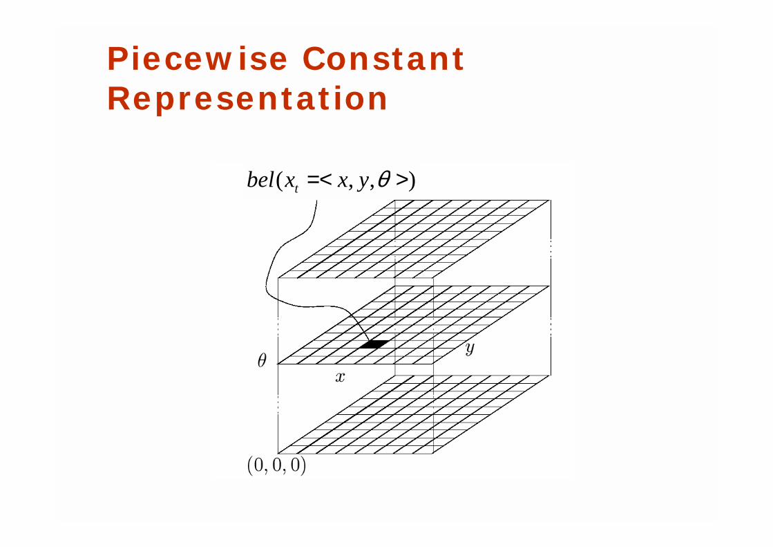
Piecewise Constant Representation

),,( >=< θyxxbel t

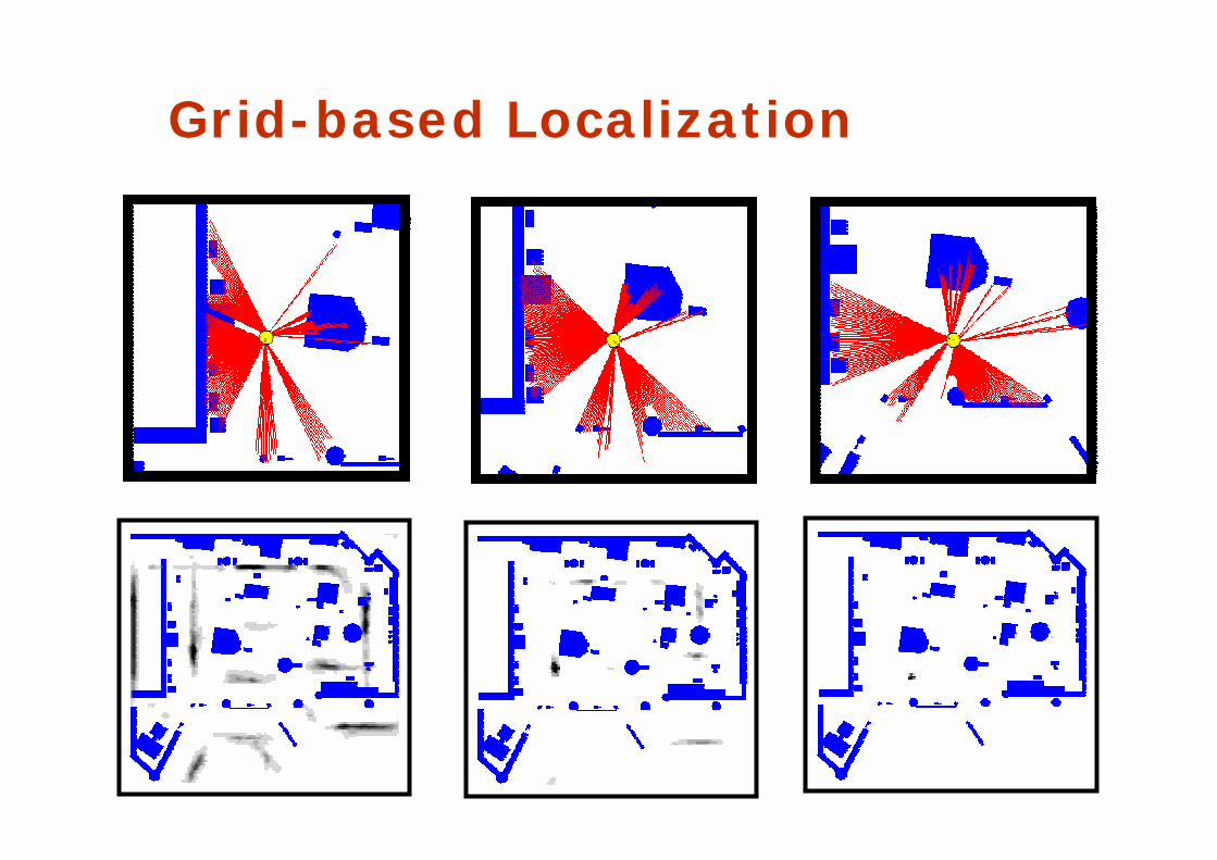
Grid-based Localization

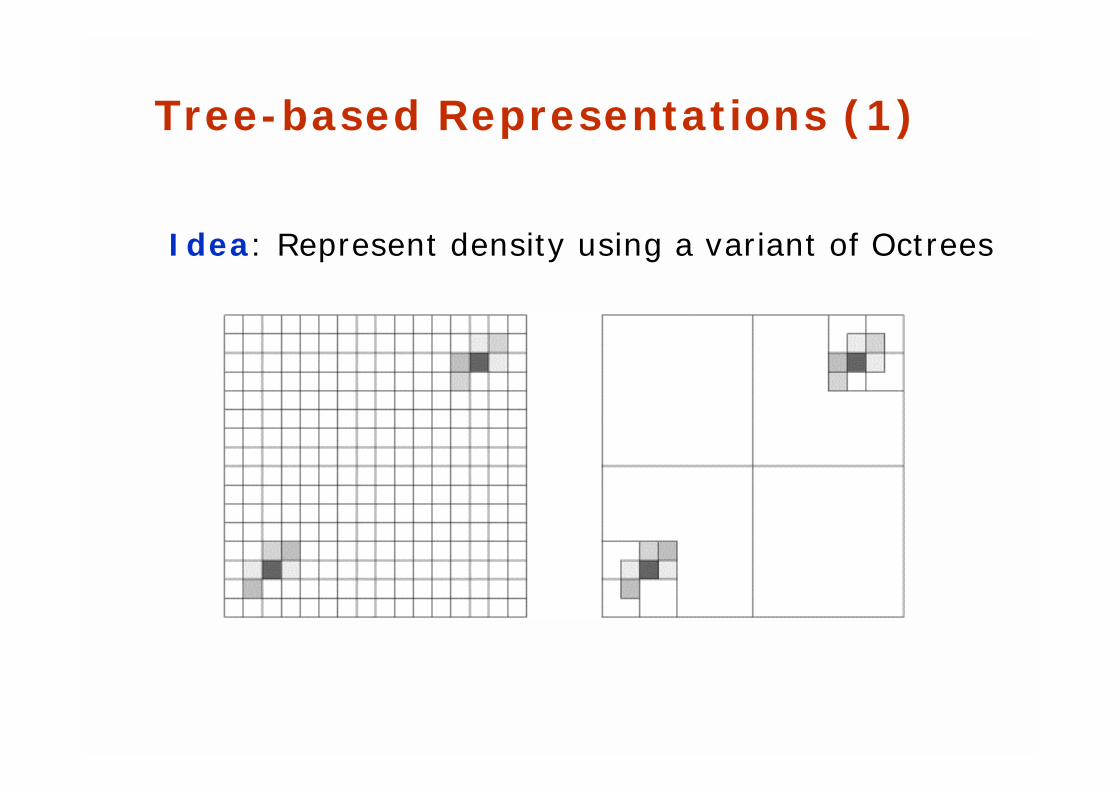
Tree-based Representations (1)

Idea: Represent density using a variant of Octrees

Xavier:Localization in a Topological Map

[Simmons and Koenig 96]

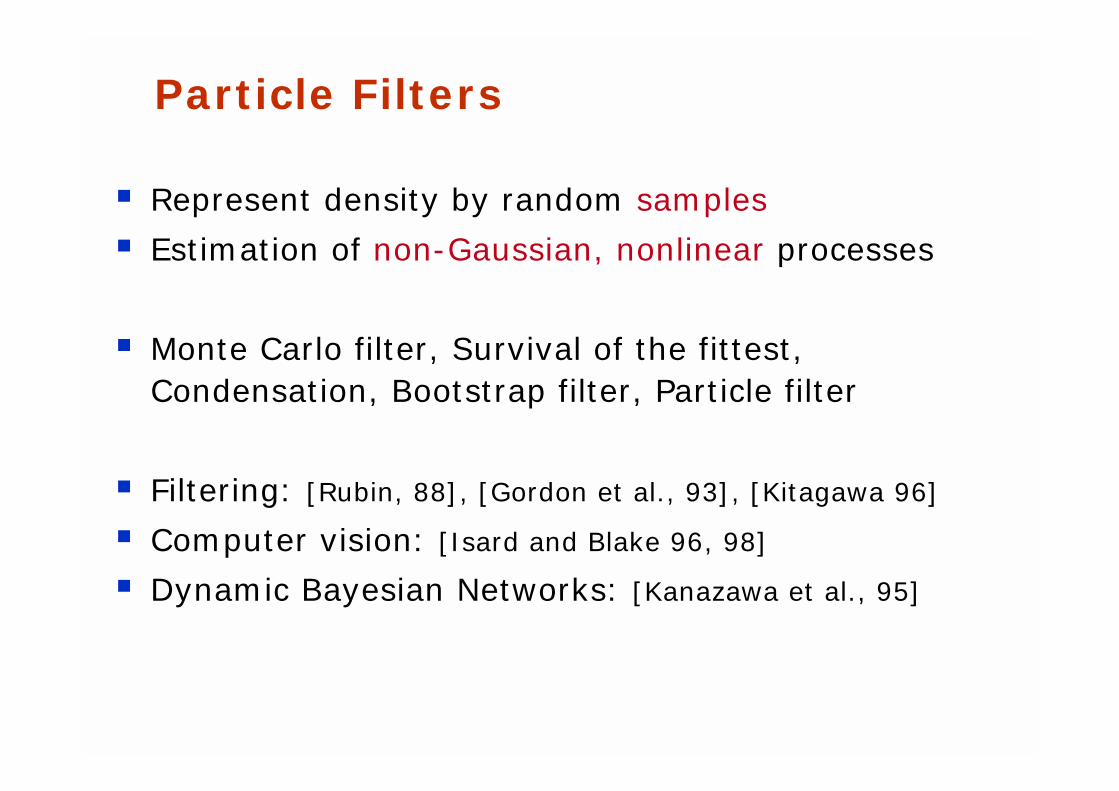
# Represent density by random samples

# Estimation of non-Gaussian, nonlinear processes

# Monte Carlo filter, Survival of the fittest, Condensation, Bootstrap filter, Particle filter

# Filtering: [Rubin, 88], [Gordon et al., 93], [Kitagawa 96]

# Computer vision: [Isard and Blake 96, 98]

# Dynamic Bayesian Networks: [Kanazawa et al., 95]

Particle Filters

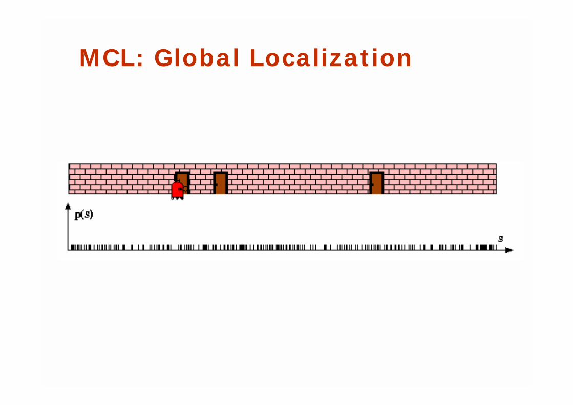
MCL: Global Localization

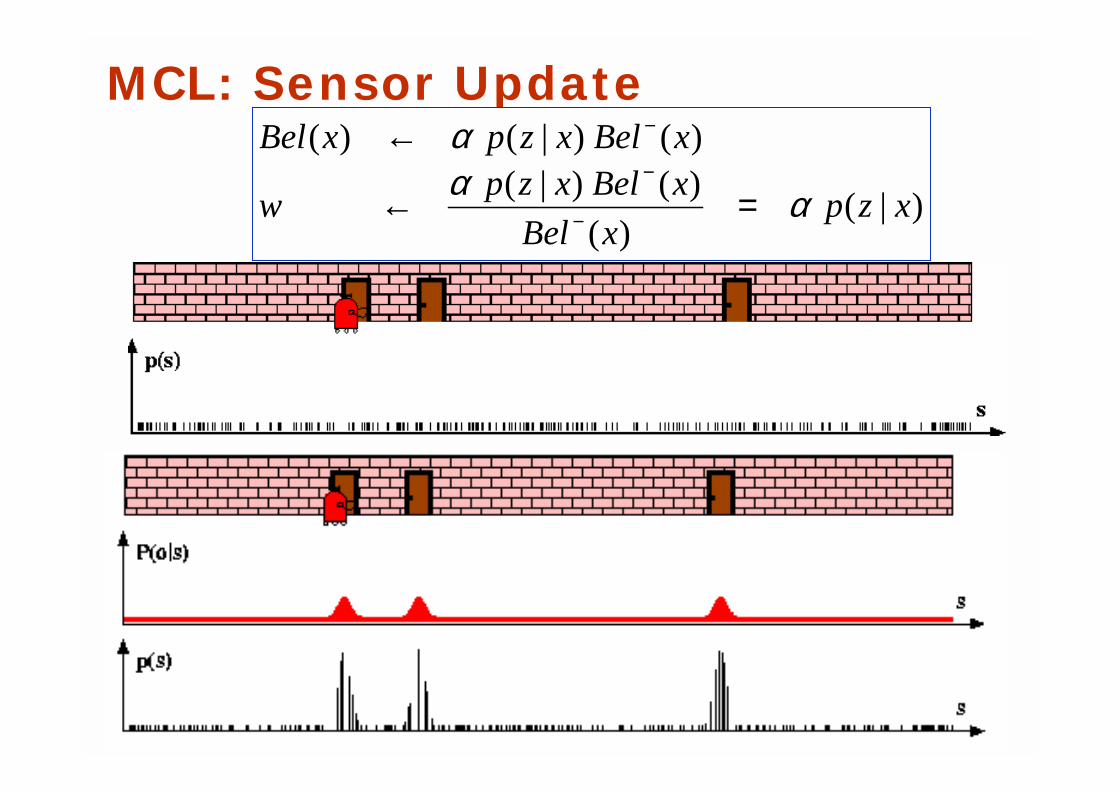
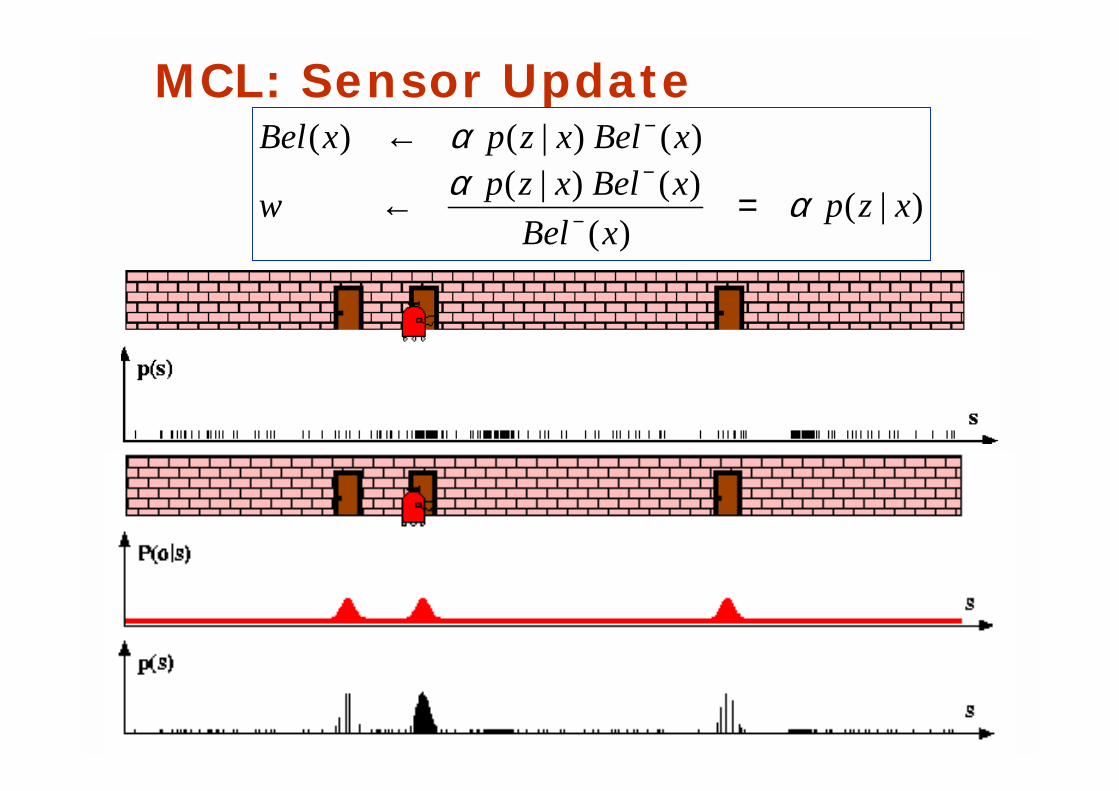
MCL: Sensor Update

)|()(

)()|()()|()(

xzpxBel

xBelxzpw

xBelxzpxBel

ααα

=←

←

−

−

−

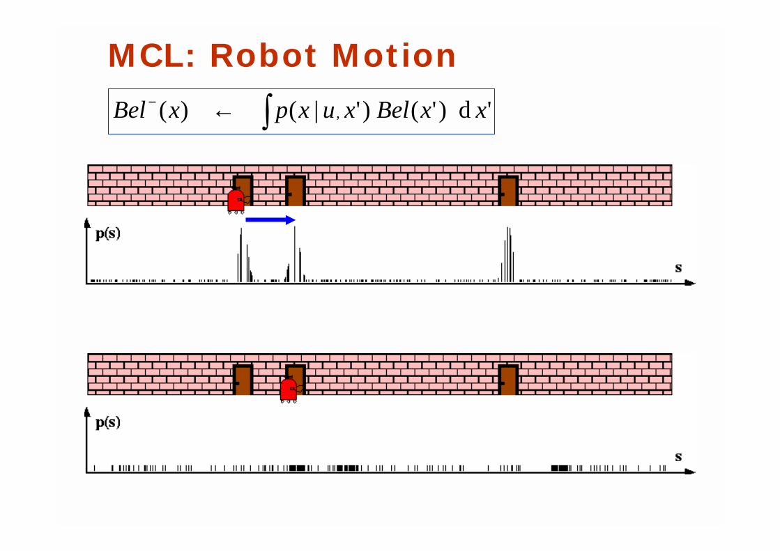
MCL: Robot Motion

∫←− 'd)'()'|()( , xxBelxuxpxBel

)|()(

)()|()()|()(

xzpxBel

xBelxzpw

xBelxzpxBel

ααα

=←

←

−

−

−

MCL: Sensor Update

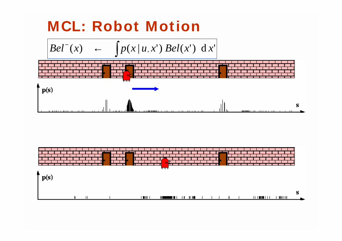
MCL: Robot Motion

∫←− 'd)'()'|()( , xxBelxuxpxBel

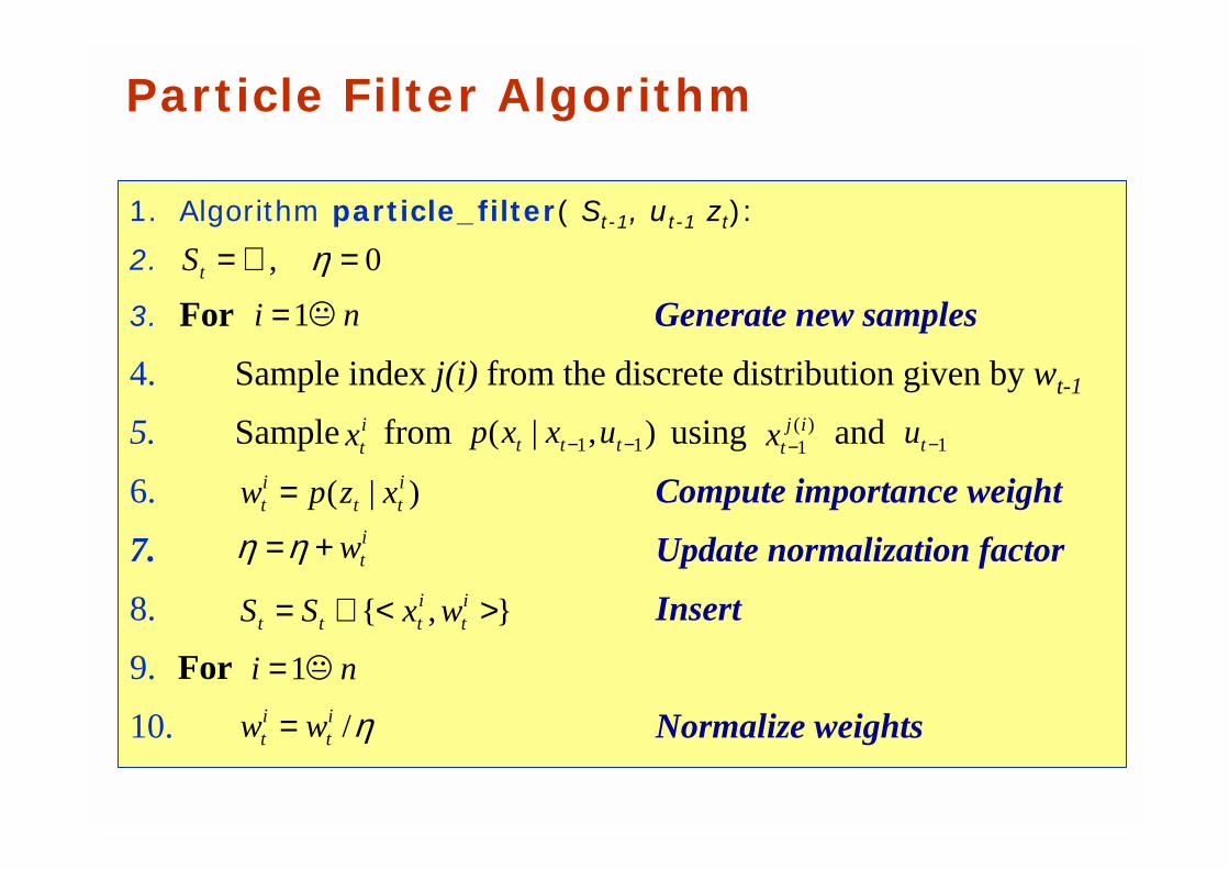
1. Algorithm particle_filter( St-1, ut-1 zt):

2.

3. For Generate new samples

4. Sample index j(i) from the discrete distribution given by wt-1

5. Sample from using and

6. Compute importance weight

7. Update normalization factor

8. Insert

9. For

10. Normalize weights

Particle Filter Algorithm

0, =∅= ηtS

ni "1=

},{ ><∪= it

ittt wxSS

itw+=ηη

itx ),|( 11 −− ttt uxxp )(

1ij

tx − 1−tu

)|( itt

it xzpw =

ni "1=

η/it

it ww =

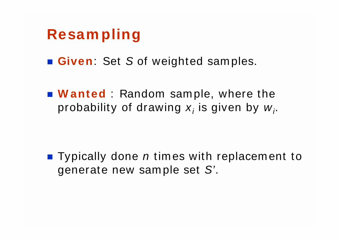
Resampling

! Given: Set S of weighted samples.

! Wanted : Random sample, where the probability of drawing xi is given by wi.

! Typically done n times with replacement to generate new sample set S’.

w2

w3

w1wn

Wn-1

Resampling

w2

w3

w1wn

Wn-1

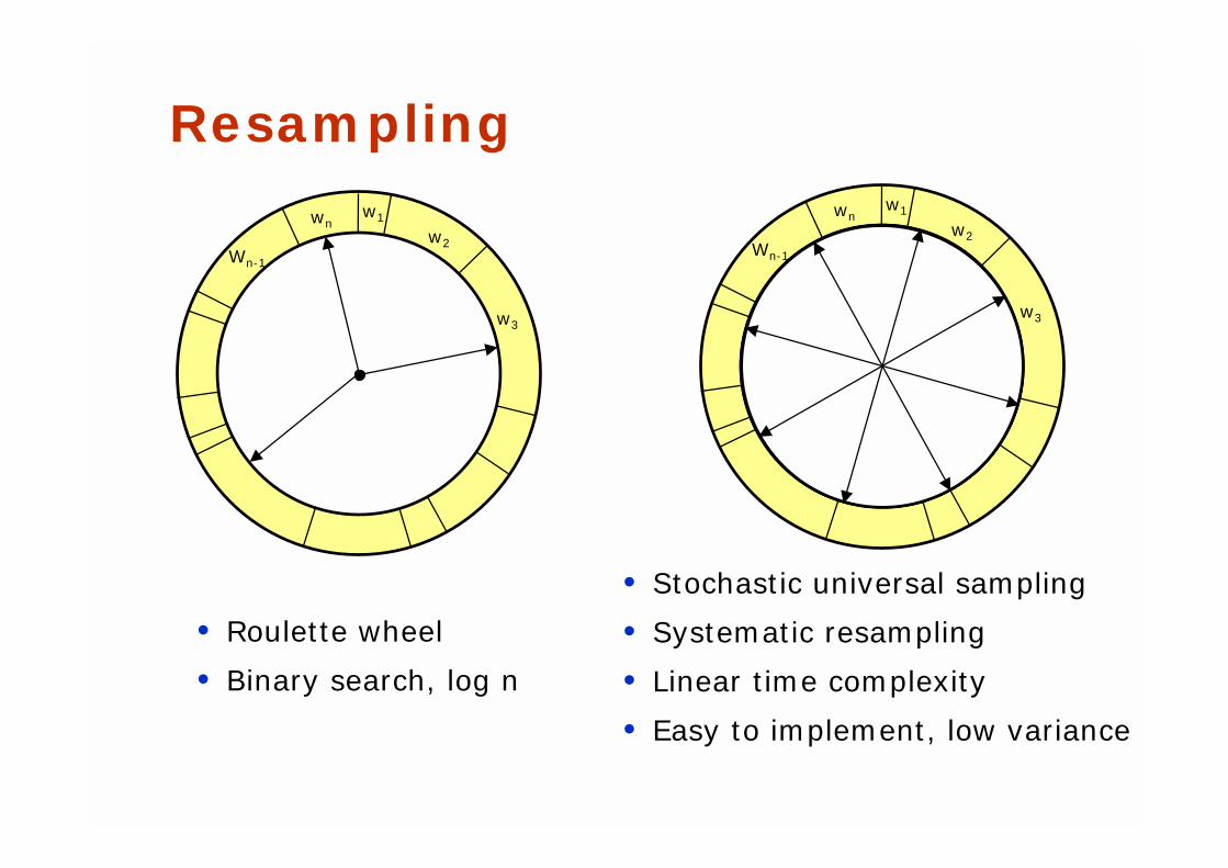
• Roulette wheel

• Binary search, log n

• Stochastic universal sampling

• Systematic resampling

• Linear time complexity

• Easy to implement, low variance

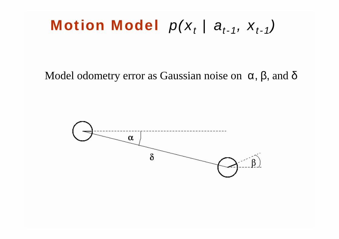
Motion Model p(xt | at-1, xt-1)

Model odometry error as Gaussian noise on α, β, and δ

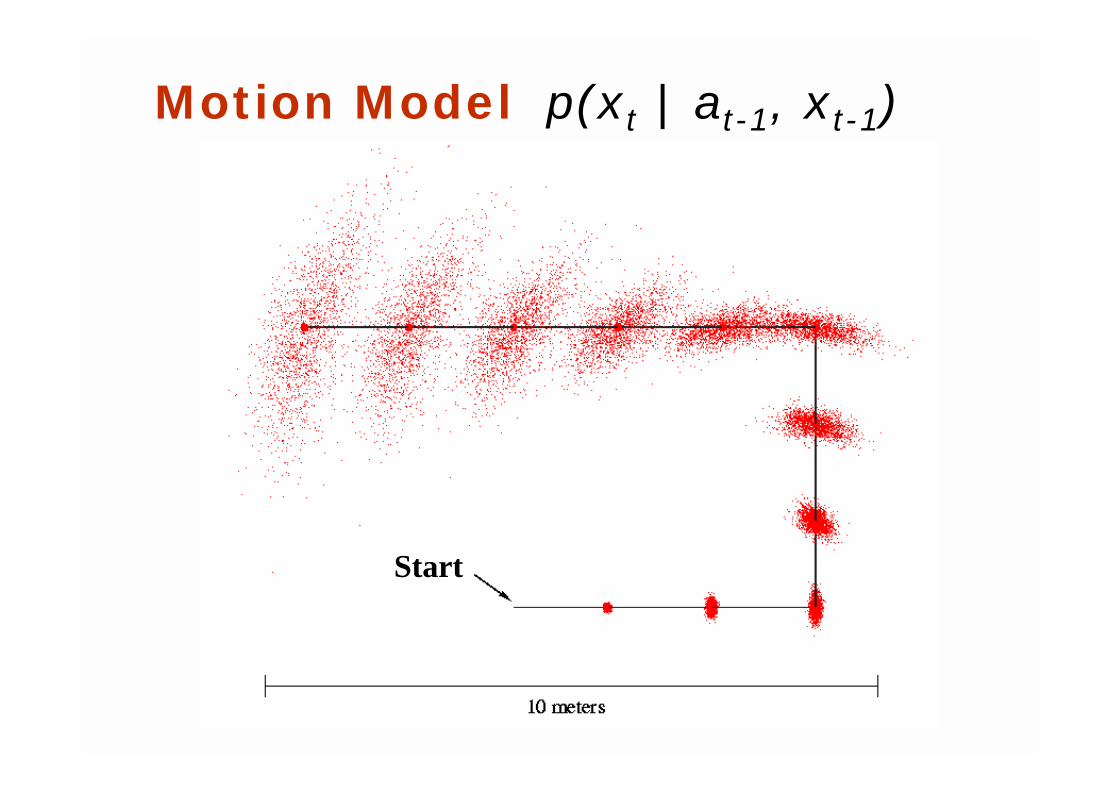
Start

Motion Model p(xt | at-1, xt-1)

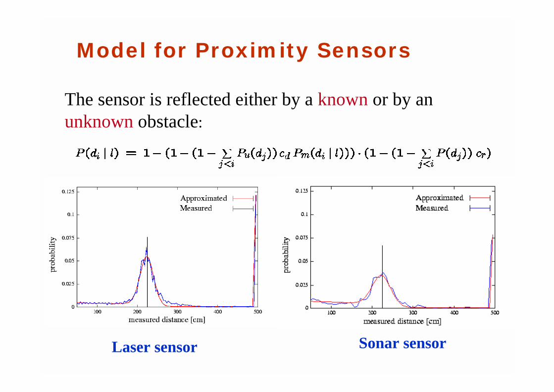
Model for Proximity Sensors

The sensor is reflected either by a known or by anunknown obstacle:

Laser sensor Sonar sensor

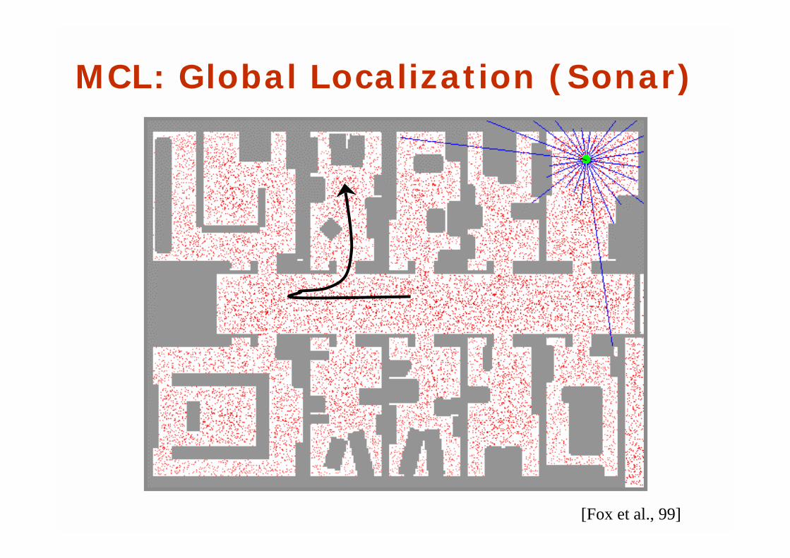
[Fox et al., 99]

MCL: Global Localization (Sonar)

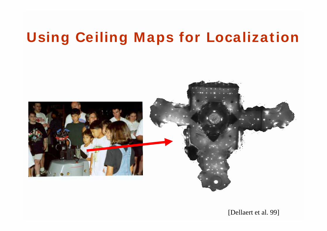
Using Ceiling Maps for Localization

[Dellaert et al. 99]

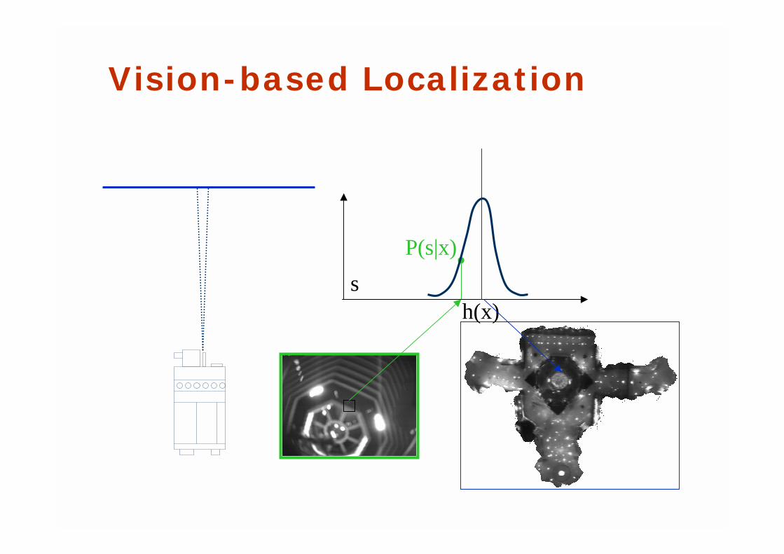
Vision-based Localization

P(s|x)

h(x)s

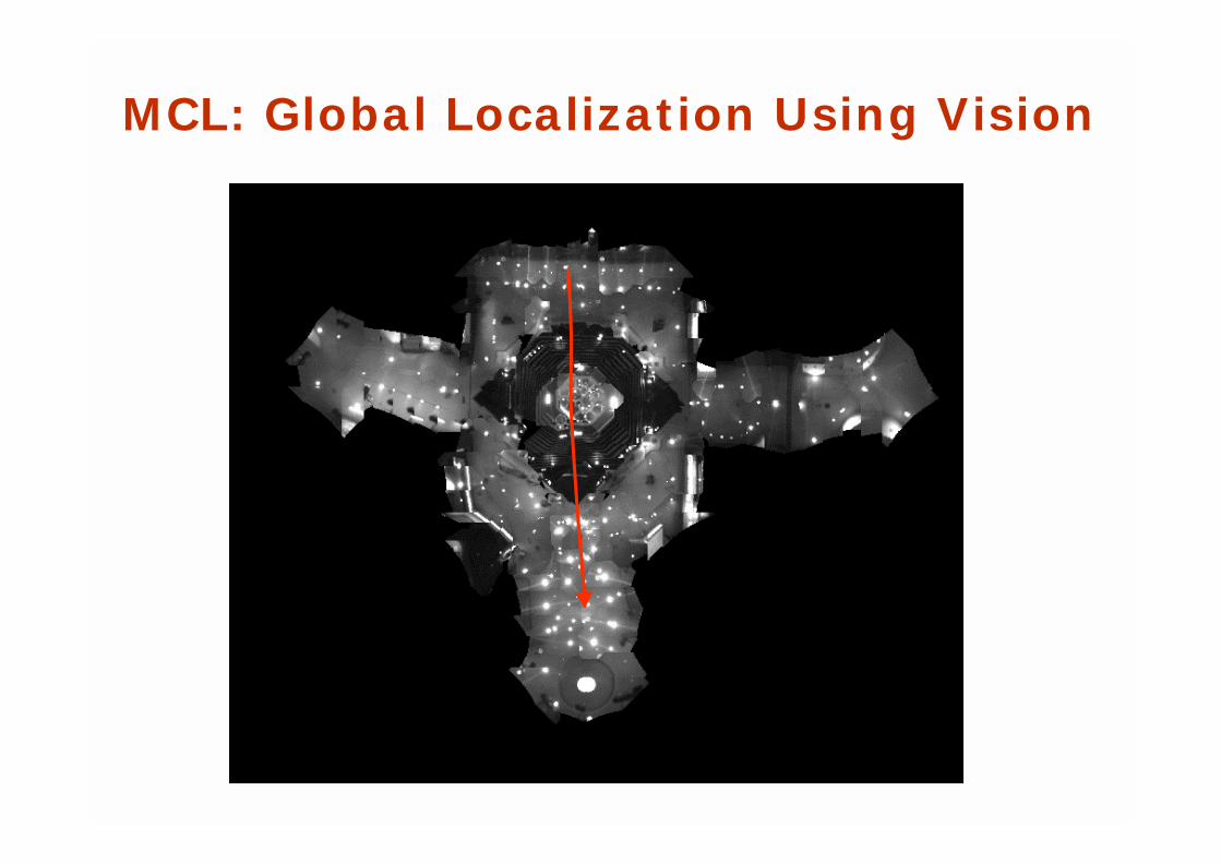
MCL: Global Localization Using Vision

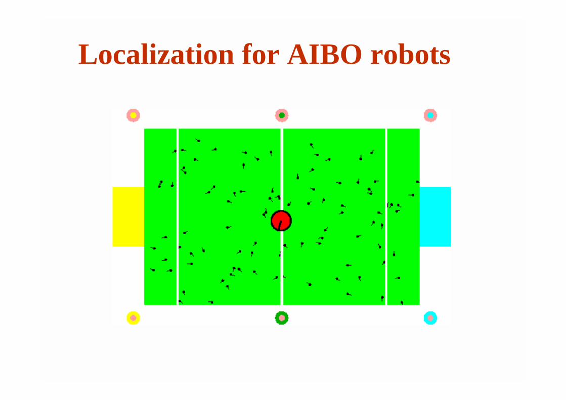
Localization for AIBO robots

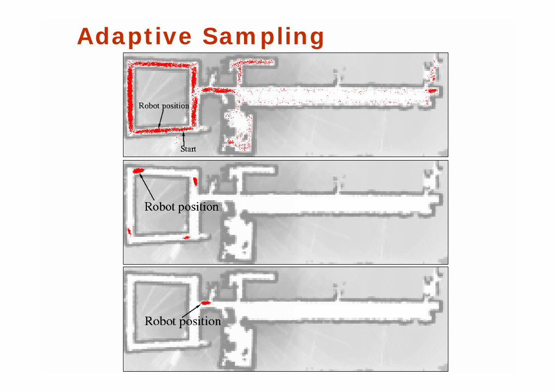
Adaptive Sampling

• Idea: • Assume we know the true belief.

• Represent this belief as a multinomial distribution.

• Determine number of samples such that we can guarantee that, with probability (1- δ), the KL-distance between the true posterior and the sample-based approximation is less than ε.

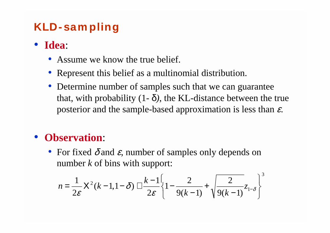
• Observation: • For fixed δ and ε, number of samples only depends on

number k of bins with support:

KLD-sampling

3

12

)1(9

2

)1(9

21

2

1)1,1(

2

1

−+

−−−≅−−Χ= −δε

δε

zkk

kkn

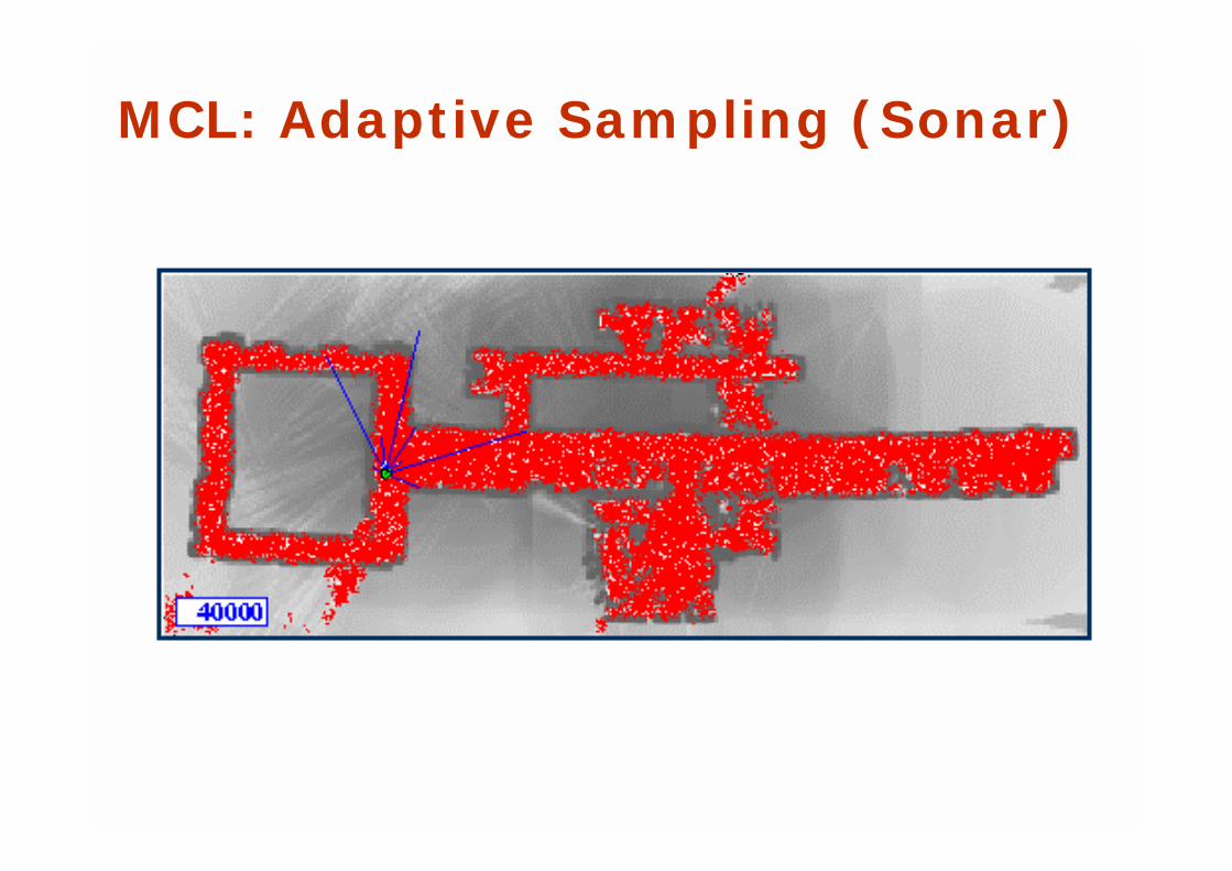
MCL: Adaptive Sampling (Sonar)

Particle Filters for Robot Localization (Summary)

! Approximate Bayes Estimation/Filtering! Full posterior estimation

! Converges in O(1/√#samples) [Tanner’93]

! Robust: multiple hypotheses with degree of belief

! Efficient in low-dimensional spaces: focuses computation where needed

! Any-time: by varying number of samples

! Easy to implement

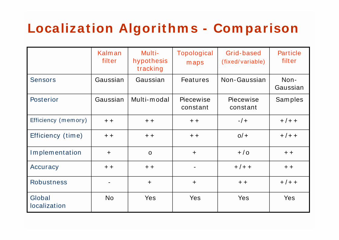
Localization Algorithms - Comparison

Non-Gaussian

Non-GaussianFeaturesGaussianGaussianSensors

+/++++++-Robustness

+++/++-++++Accuracy

+/++-/+++++++Efficiency (memory)

Yes

+/o

o/+

Piecewise constant

Grid-based(fixed/variable)

+/++++++++Efficiency (time)

+++o+Implementation

SamplesPiecewise constant

Multi-modalGaussianPosterior

YesYesYesNoGlobal localization

Multi-hypothesis tracking

Particle filter

Topologicalmaps

Kalman filter

Localization: Lessons Learned

! Probabilistic Localization = Bayes filters! Particle filters: Approximate posterior

by random samples! Extensions:

! Filter for dynamic environments! Safe avoidance of invisible hazards! People tracking! Recovery from total failures! Active Localization! Multi-robot localization