Revision of JN-RM-3106-07

Recurrent neural networks trained in the presence of noisegive rise to mixed muscle-movement representations

Emanuel Todorov

Department of Cognitive Science

University of California San Diego

La Jolla, CA 92093-0515

todorov@cogsci.ucsd.edu

Section: Behavioral/Systems/Cognitive

Number of figures: 6

Number of tables: 1

Number of pages: 30

Keywords: primary motor cortex, mixed muscle-movement representation, recurrent neural

network, stochastic optimal control, backpropagation-through-time, motor redundancy

Acknowledgements

This work was supported by the US National Institutes of Health. Thanks to Shinji Kakei, Donna

Hoffman and Peter Strick for making their data available.

1

Abstract

Primary motor cortex was found to use a mixed muscle-movement representation, further compli-

cating the debates regarding its role in movement production. Here we show that such a mixed

representation corresponds to the optimal way of computing muscle activity given reach targets

and arm postures. The key determinant of what representation is optimal turns out to be neural

noise, and in particular the diversity of neural noise. The model is a stochastic recurrent network

trained on a cost function which is defined in terms of muscle activity rather than neural activity.

Since there are more neurons than muscles, the computation involves a large amount of redundancy.

However this redundancy can be resolved because few of the networks capable of such computation

are robust to noise. Although these networks differ in their detail, they all use a similar representa-

tion. We have previously combined the ideas of optimality and noise to address redundancy on the

biomechanical level. The present work extends this approach to the neural level, where redundancy

is much larger and yet has rarely been addressed in a principled manner.

2

Introduction

While the critical role of primary motor cortex (M1) in the production of voluntary movement is

well established, precisely what that role is remains a matter of debate. Early studies in awake

behaving monkeys performing single-joint tasks suggested that M1 activity is closely related to

muscle activity [Evarts, 1981]. Later observations from multi-joint tasks challenged this view and

led to the alternative notion that M1 represents more abstract movement features, in particular

movement direction [Georgopoulos et al., 1982]. A number of subsequent studies showed that

pretty much anything related to movement appears to be represented in M1, begging the question

of whether the search for such representations is a worthwhile endeavor [Fetz, 1992]. Worthwhile

or not, the resulting debates tend to be heated [Moran et al., 2000,Krutzer et al., 2007].

One of these debates was triggered by our attempt [Todorov, 2000] to explain many disparate

findings by assuming that M1 controls muscles while compensating for the position- and velocity-

dependence in muscle force production. The present paper extends this earlier model while ad-

dressing a general shortcoming of many studies in systems neuroscience — which is that they focus

on neural representations and largely ignore the underlying computations. Such focus is partly

understandable given that representations are more directly accessible experimentally. Yet it has

the flavor of seeking the key in the wrong place just because the wrong place is better illuminated.

The above criticism also applies to our earlier work where we focused on the relation between M1

output and muscle activity but said little about how M1 computes its output given its input. Here

we fill this gap: we specify the input to our M1 model together with the desired pattern of muscle

activity, and let the computational mechanisms as well as the associated neural representations

emerge from optimization of stochastic recurrent networks.

The specific motivation behind the new model is the qualitative difference between M1 and

muscle activity observed in experiments where monkeys made wrist movements in different fore-

arm postures [Kakei et al., 1999, Yanai et al., 2007]. These studies are important because they

were perfectly designed to resolve the long-standing controversy about muscle versus movement

representations in M1, but instead of resolving the controversy the data seemed to contradict both

views. Muscle preferred directions (PDs) were substantially affected by posture and shifted as

much as muscle pulling directions, as one would expect from biomechanics and energy minimiza-

tion [Todorov, 2002]. In contrast, PDs in M1 shifted only about half as much. The directional

coding hypothesis [Georgopoulos et al., 1983] predicts an absence of a systematic PD shift, while

3

the muscle control hypothesis seems more consistent with an equal amount of shift in M1 and

muscles. Posture also affected the gains in both M1 and muscles [Kakei et al., 1999]. Technically

these gain changes are sufficient to rescue the muscle control hypothesis [Todorov, 2000,Todorov,

2003, Kakei et al., 2003, Shah et al., 2004], using a mechanism we call "projection" (see below).

Conceptually, however, this dataset presents a challenge: if M1 controls muscles then why does it

behave differently from muscles? The general answer we propose is "redundancy + optimality".

Any pattern of muscle activity can be elicited by an infinite variety of M1 representations, and

the representation "chosen" through learning is optimized to get a job done rather than be intu-

itive [Fetz, 1992]. We show that optimizing recurrent networks to transform reach targets and arm

postures into muscle activations gives rise to a mixed muscle-movement representation similar to

the one observed experimentally. Extensive simulations indicate that this solution corresponds to

the global minimum and is robust with respect to a wide range of parameter changes.

The notion of redundancy has played a key role in motor control since Bernstein [Bernstein,

1967]. It has usually been applied to the level of biomechanics, leading to questions such as how do

we select one out of the many combinations of arm joint angles bringing the fingertip to the same

location in space [Scholz and Schoner, 1999]. Optimality principles have been very successful in

explaining how the brain deals with biomechanical redundancy [Todorov, 2004]. Taking noise into

account has proven essential in such models [Harris and Wolpert, 1998,Todorov and Jordan, 2002].

For example, we showed that stochastic optimal control leads to a minimal intervention strategy

suppressing task-relevant disturbances while leaving task-irrelevant ones uncorrected. This enabled

us to get away from the notion of desired trajectories and account for the patterns of movement

variability observed in redundant tasks [Scholz and Schoner, 1999,Todorov and Jordan, 2002]. Here

we extend optimality principles to the neural level and use them to resolve neural redundancy.

Perhaps the most interesting finding is that noise turns out to be equally essential on the neural

level, although the specific reasons appear to be different. When we train networks in the presence

of heterogeneous neural noise, training gives rise to the mixed muscle-movement representation

found in M1 and leads to a number of additional desirable properties. In contrast, when we

train the same networks under deterministic conditions, the results are qualitatively different and

biologically implausible. To solve the challenging optimization problems arising in this study, we

extend the backpropagation-through-time algorithm [Hertz et al., 1991] in a way which makes

training stochastic recurrent networks almost as efficient as training deterministic ones.

4

Methods

The Methods section appears before Results to comply with the journal style. However this ordering

is geared towards experimental studies and tends to be unsuitable for presenting theoretical work.

The reader may want to skip to Results and refer to Methods for details when necessary.

Network architecture

A stochastic recurrent network is given two external inputs coding the reach target in extrinsic space

and the forearm posture, and is trained to produce the muscle activity needed to initiate movement.

The network hasN neurons each labeled with an input preferred direction yn ∈ [−180◦, 180◦] and an

input postural gradient xn ∈ {−1,+1}. The values of yn are uniformly distributed and uncorrelated

with xn. Together yn and xn determine the external input to neuron n as follows. Let x ∈ [−1, 1]

denote the forearm posture on a given trial, while y ∈ [−180◦, 180◦] and m ∈ [0,mmax] denote

the extrinsic direction and amplitude of movement to the desired target. Then the (deterministic

component of the) external input to neuron n is

wYm (1 + cos (yn − y)) + wXmmax (1 + xnx)

wY and wX are shared weights which are the same for all neurons. Adding 1 to the terms

cos (yn − y) and xnx makes all external inputs non-negative. Scaling the postural term by mmax

makes the influence of the posture and target inputs comparable. The task variables m, y, x vary

between trials (uniformly in their respective range) but remain constant within a trial. In addition

to the external input, each neuron n also receives bias input wBn as well as time-varying recurrent

input wRn,kok (t) from every other neuron k. The output of neuron k at time step t is denoted ok (t)

and the recurrent weight from k to n is denoted wRn,k. Keep in mind that the network dynamics

can give rise to recurrent inputs which are different from the external inputs, thus the tuning of a

neuron’s response may be different from the tuning of its external inputs.

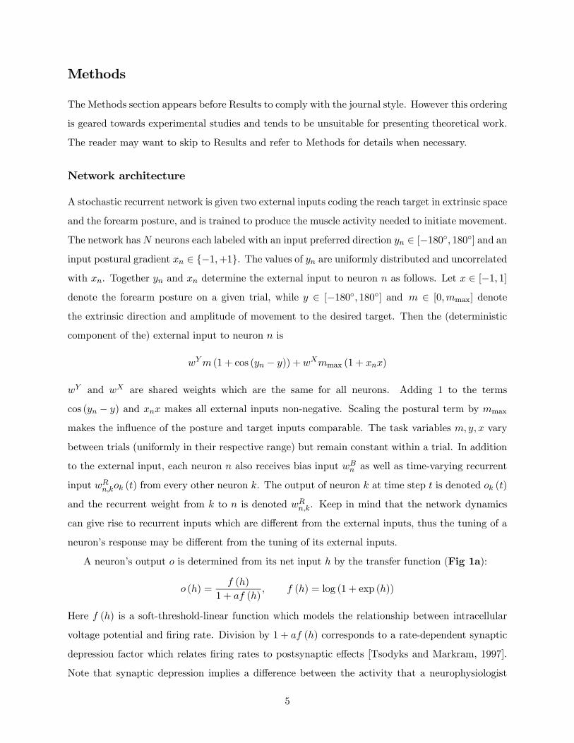
A neuron’s output o is determined from its net input h by the transfer function (Fig 1a):

o (h) =f (h)

1 + af (h), f (h) = log (1 + exp (h))

Here f (h) is a soft-threshold-linear function which models the relationship between intracellular

voltage potential and firing rate. Division by 1 + af (h) corresponds to a rate-dependent synaptic

depression factor which relates firing rates to postsynaptic effects [Tsodyks and Markram, 1997].

Note that synaptic depression implies a difference between the activity that a neurophysiologist

5

records extracellularly and the activity that postsynaptic neurons receive from the same neuron.

In the text h is called input, f (h) is called firing rate, and o (h) is called output. The reason for

using the above transfer function instead of a more standard sigmoid is because it adds biological

realism without complicating the model.

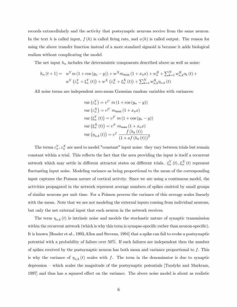
The net input hn includes the deterministic components described above as well as noise:

hn (t+ 1) = wYm (1 + cos (yn − y)) + wXmmax (1 + xnx) + wBn +

PNk=1w

Rn,kok (t)+

wY¡εYn + ξYn (t)

¢+ wX

¡εXn + ξXn (t)

¢+PN

k=1wRn,kηn,k (t)

All noise terms are independent zero-mean Gaussian random variables with variances:

var¡εYn¢= υC m (1 + cos (yn − y))

var¡εXn¢= υC mmax (1 + xnx)

var¡ξYn (t)

¢= υF m (1 + cos (yn − y))

var¡ξXn (t)

¢= υF mmax (1 + xnx)

var¡ηn,k (t)

¢= υI

f (hk (t))

(1 + af (hk (t)))2

The terms εYn , εXn are used to model "constant" input noise: they vary between trials but remain

constant within a trial. This reflects the fact that the area providing the input is itself a recurrent

network which may settle in different attractor states on different trials. ξYn (t) , ξXn (t) represent

fluctuating input noise. Modeling variance as being proportional to the mean of the corresponding

input captures the Poisson nature of cortical activity. Since we are using a continuous model, the

activities propagated in the network represent average numbers of spikes emitted by small groups

of similar neurons per unit time. For a Poisson process the variance of this average scales linearly

with the mean. Note that we are not modeling the external inputs coming from individual neurons,

but only the net external input that each neuron in the network receives.

The term ηn,k (t) is intrinsic noise and models the stochastic nature of synaptic transmission

within the recurrent network (which is why this term is synapse-specific rather than neuron-specific).

It is known [Hessler et al., 1993,Allen and Stevens, 1994] that a spike can fail to evoke a postsynaptic

potential with a probability of failure over 50%. If such failures are independent then the number

of spikes received by the postsynaptic neuron has both mean and variance proportional to f . This

is why the variance of ηn,k (t) scales with f . The term in the denominator is due to synaptic

depression — which scales the magnitude of the postsynaptic potentials [Tsodyks and Markram,

1997] and thus has a squared effect on the variance. The above noise model is about as realistic

6

as it can be given the continuous neuronal dynamics. A spiking network would allow even more

realistic noise but would be very hard to train.

In the absence of task-related input (that is, when wY = wX = 0) the neurons have neuron-

specific baselines due to the different biases wBn . To avoid initial transients, this baseline activity

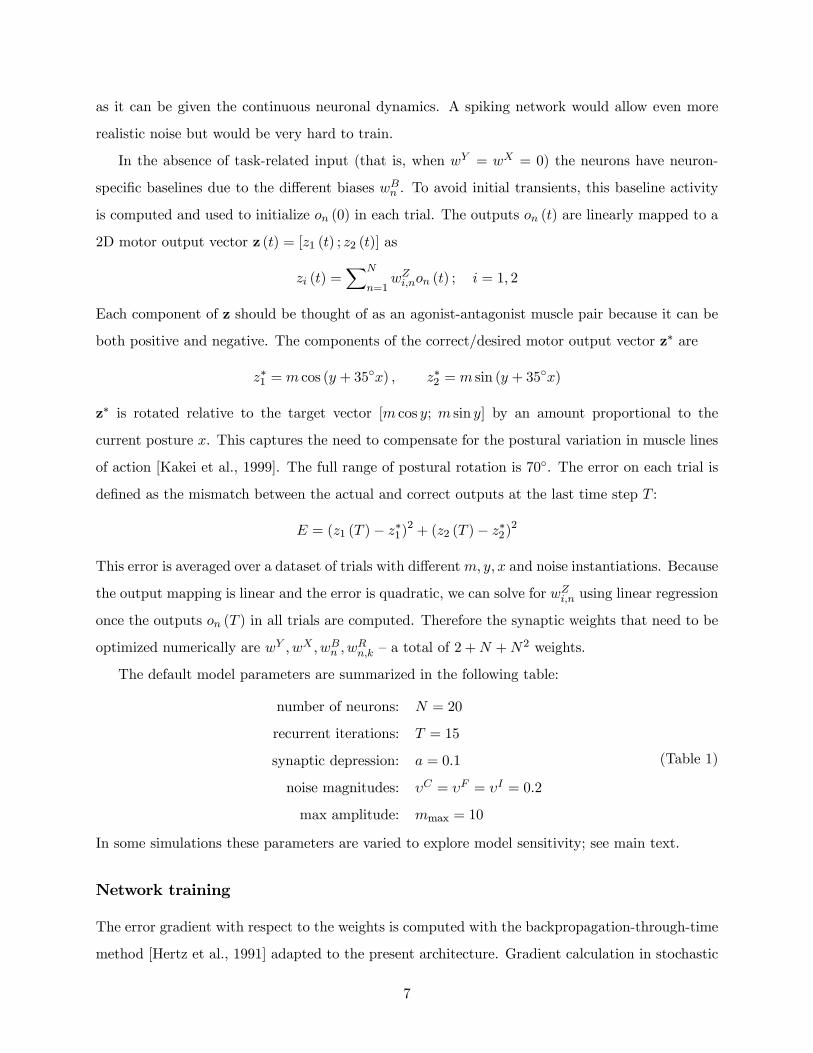
is computed and used to initialize on (0) in each trial. The outputs on (t) are linearly mapped to a

2D motor output vector z (t) = [z1 (t) ; z2 (t)] as

zi (t) =XN

n=1wZi,non (t) ; i = 1, 2

Each component of z should be thought of as an agonist-antagonist muscle pair because it can be

both positive and negative. The components of the correct/desired motor output vector z∗ are

z∗1 = m cos (y + 35◦x) , z∗2 = m sin (y + 35◦x)

z∗ is rotated relative to the target vector [m cos y; m sin y] by an amount proportional to the

current posture x. This captures the need to compensate for the postural variation in muscle lines

of action [Kakei et al., 1999]. The full range of postural rotation is 70◦. The error on each trial is

defined as the mismatch between the actual and correct outputs at the last time step T :

E = (z1 (T )− z∗1)2 + (z2 (T )− z∗2)

2

This error is averaged over a dataset of trials with differentm, y, x and noise instantiations. Because

the output mapping is linear and the error is quadratic, we can solve for wZi,n using linear regression

once the outputs on (T ) in all trials are computed. Therefore the synaptic weights that need to be

optimized numerically are wY , wX , wBn , w

Rn,k — a total of 2 +N +N2 weights.

The default model parameters are summarized in the following table:

number of neurons: N = 20

recurrent iterations: T = 15

synaptic depression: a = 0.1

noise magnitudes: υC = υF = υI = 0.2

max amplitude: mmax = 10

(Table 1)

In some simulations these parameters are varied to explore model sensitivity; see main text.

Network training

The error gradient with respect to the weights is computed with the backpropagation-through-time

method [Hertz et al., 1991] adapted to the present architecture. Gradient calculation in stochastic

7

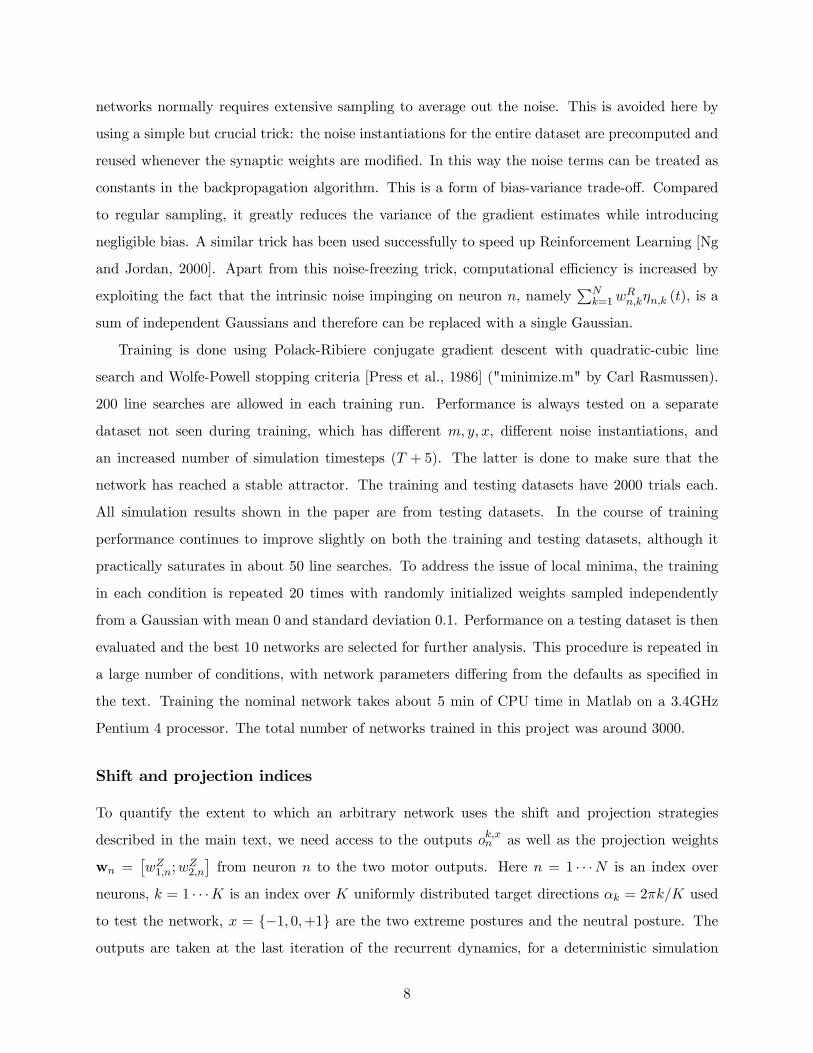
networks normally requires extensive sampling to average out the noise. This is avoided here by

using a simple but crucial trick: the noise instantiations for the entire dataset are precomputed and

reused whenever the synaptic weights are modified. In this way the noise terms can be treated as

constants in the backpropagation algorithm. This is a form of bias-variance trade-off. Compared

to regular sampling, it greatly reduces the variance of the gradient estimates while introducing

negligible bias. A similar trick has been used successfully to speed up Reinforcement Learning [Ng

and Jordan, 2000]. Apart from this noise-freezing trick, computational efficiency is increased by

exploiting the fact that the intrinsic noise impinging on neuron n, namelyPN

k=1wRn,kηn,k (t), is a

sum of independent Gaussians and therefore can be replaced with a single Gaussian.

Training is done using Polack-Ribiere conjugate gradient descent with quadratic-cubic line

search and Wolfe-Powell stopping criteria [Press et al., 1986] ("minimize.m" by Carl Rasmussen).

200 line searches are allowed in each training run. Performance is always tested on a separate

dataset not seen during training, which has different m, y, x, different noise instantiations, and

an increased number of simulation timesteps (T + 5). The latter is done to make sure that the

network has reached a stable attractor. The training and testing datasets have 2000 trials each.

All simulation results shown in the paper are from testing datasets. In the course of training

performance continues to improve slightly on both the training and testing datasets, although it

practically saturates in about 50 line searches. To address the issue of local minima, the training

in each condition is repeated 20 times with randomly initialized weights sampled independently

from a Gaussian with mean 0 and standard deviation 0.1. Performance on a testing dataset is then

evaluated and the best 10 networks are selected for further analysis. This procedure is repeated in

a large number of conditions, with network parameters differing from the defaults as specified in

the text. Training the nominal network takes about 5 min of CPU time in Matlab on a 3.4GHz

Pentium 4 processor. The total number of networks trained in this project was around 3000.

Shift and projection indices

To quantify the extent to which an arbitrary network uses the shift and projection strategies

described in the main text, we need access to the outputs ok,xn as well as the projection weights

wn =£wZ1,n;w

Z2,n

¤from neuron n to the two motor outputs. Here n = 1 · · ·N is an index over

neurons, k = 1 · · ·K is an index over K uniformly distributed target directions αk = 2πk/K used

to test the network, x = {−1, 0,+1} are the two extreme postures and the neutral posture. The

outputs are taken at the last iteration of the recurrent dynamics, for a deterministic simulation

8

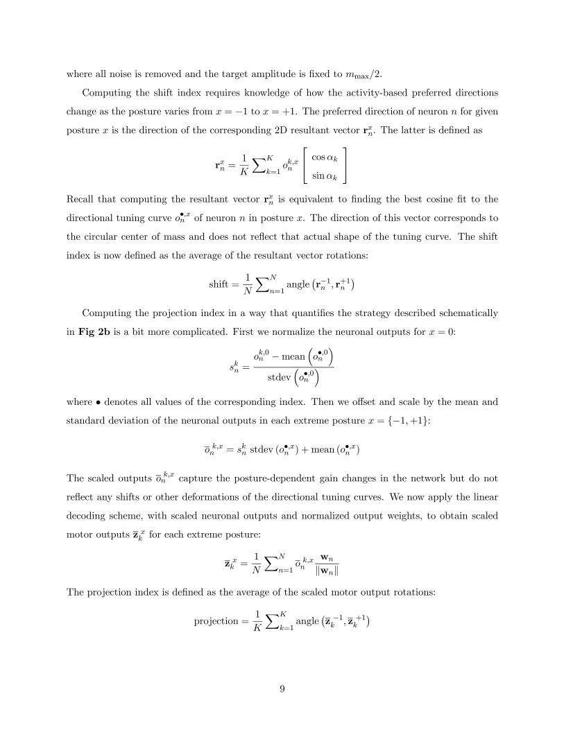
where all noise is removed and the target amplitude is fixed to mmax/2.

Computing the shift index requires knowledge of how the activity-based preferred directions

change as the posture varies from x = −1 to x = +1. The preferred direction of neuron n for given

posture x is the direction of the corresponding 2D resultant vector rxn. The latter is defined as

rxn =1

K

XK

k=1ok,xn

⎡⎣ cosαksinαk

⎤⎦Recall that computing the resultant vector rxn is equivalent to finding the best cosine fit to the

directional tuning curve o•,xn of neuron n in posture x. The direction of this vector corresponds to

the circular center of mass and does not reflect that actual shape of the tuning curve. The shift

index is now defined as the average of the resultant vector rotations:

shift =1

N

XN

n=1angle

¡r−1n , r+1n

¢Computing the projection index in a way that quantifies the strategy described schematically

in Fig 2b is a bit more complicated. First we normalize the neuronal outputs for x = 0:

skn =ok,0n −mean

³o•,0n

´stdev

³o•,0n

´where • denotes all values of the corresponding index. Then we offset and scale by the mean and

standard deviation of the neuronal outputs in each extreme posture x = {−1,+1}:

o k,xn = skn stdev (o

•,xn ) + mean (o•,xn )

The scaled outputs o k,xn capture the posture-dependent gain changes in the network but do not

reflect any shifts or other deformations of the directional tuning curves. We now apply the linear

decoding scheme, with scaled neuronal outputs and normalized output weights, to obtain scaled

motor outputs z xk for each extreme posture:

z xk =

1

N

XN

n=1o k,xn

wn

kwnk

The projection index is defined as the average of the scaled motor output rotations:

projection =1

K

XK

k=1angle

¡z −1k , z +1k

¢

9

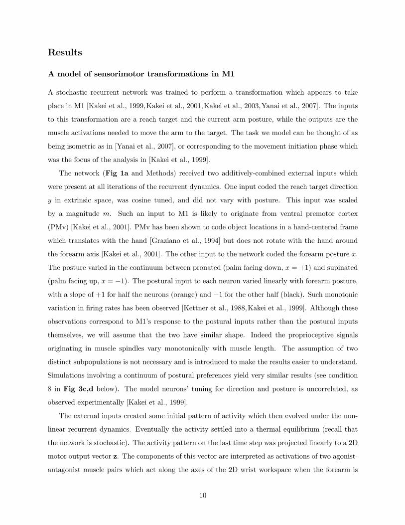
Results

A model of sensorimotor transformations in M1

A stochastic recurrent network was trained to perform a transformation which appears to take

place in M1 [Kakei et al., 1999,Kakei et al., 2001,Kakei et al., 2003,Yanai et al., 2007]. The inputs

to this transformation are a reach target and the current arm posture, while the outputs are the

muscle activations needed to move the arm to the target. The task we model can be thought of as

being isometric as in [Yanai et al., 2007], or corresponding to the movement initiation phase which

was the focus of the analysis in [Kakei et al., 1999].

The network (Fig 1a and Methods) received two additively-combined external inputs which

were present at all iterations of the recurrent dynamics. One input coded the reach target direction

y in extrinsic space, was cosine tuned, and did not vary with posture. This input was scaled

by a magnitude m. Such an input to M1 is likely to originate from ventral premotor cortex

(PMv) [Kakei et al., 2001]. PMv has been shown to code object locations in a hand-centered frame

which translates with the hand [Graziano et al., 1994] but does not rotate with the hand around

the forearm axis [Kakei et al., 2001]. The other input to the network coded the forearm posture x.

The posture varied in the continuum between pronated (palm facing down, x = +1) and supinated

(palm facing up, x = −1). The postural input to each neuron varied linearly with forearm posture,

with a slope of +1 for half the neurons (orange) and −1 for the other half (black). Such monotonic

variation in firing rates has been observed [Kettner et al., 1988,Kakei et al., 1999]. Although these

observations correspond to M1’s response to the postural inputs rather than the postural inputs

themselves, we will assume that the two have similar shape. Indeed the proprioceptive signals

originating in muscle spindles vary monotonically with muscle length. The assumption of two

distinct subpopulations is not necessary and is introduced to make the results easier to understand.

Simulations involving a continuum of postural preferences yield very similar results (see condition

8 in Fig 3c,d below). The model neurons’ tuning for direction and posture is uncorrelated, as

observed experimentally [Kakei et al., 1999].

The external inputs created some initial pattern of activity which then evolved under the non-

linear recurrent dynamics. Eventually the activity settled into a thermal equilibrium (recall that

the network is stochastic). The activity pattern on the last time step was projected linearly to a 2D

motor output vector z. The components of this vector are interpreted as activations of two agonist-

antagonist muscle pairs which act along the axes of the 2D wrist workspace when the forearm is

10

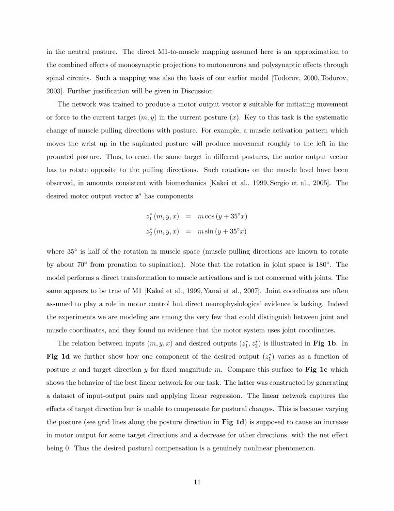
in the neutral posture. The direct M1-to-muscle mapping assumed here is an approximation to

the combined effects of monosynaptic projections to motoneurons and polysynaptic effects through

spinal circuits. Such a mapping was also the basis of our earlier model [Todorov, 2000,Todorov,

2003]. Further justification will be given in Discussion.

The network was trained to produce a motor output vector z suitable for initiating movement

or force to the current target (m, y) in the current posture (x). Key to this task is the systematic

change of muscle pulling directions with posture. For example, a muscle activation pattern which

moves the wrist up in the supinated posture will produce movement roughly to the left in the

pronated posture. Thus, to reach the same target in different postures, the motor output vector

has to rotate opposite to the pulling directions. Such rotations on the muscle level have been

observed, in amounts consistent with biomechanics [Kakei et al., 1999, Sergio et al., 2005]. The

desired motor output vector z∗ has components

z∗1 (m, y, x) = m cos (y + 35◦x)

z∗2 (m, y, x) = m sin (y + 35◦x)

where 35◦ is half of the rotation in muscle space (muscle pulling directions are known to rotate

by about 70◦ from pronation to supination). Note that the rotation in joint space is 180◦. The

model performs a direct transformation to muscle activations and is not concerned with joints. The

same appears to be true of M1 [Kakei et al., 1999,Yanai et al., 2007]. Joint coordinates are often

assumed to play a role in motor control but direct neurophysiological evidence is lacking. Indeed

the experiments we are modeling are among the very few that could distinguish between joint and

muscle coordinates, and they found no evidence that the motor system uses joint coordinates.

The relation between inputs (m,y, x) and desired outputs (z∗1 , z∗2) is illustrated in Fig 1b. In

Fig 1d we further show how one component of the desired output (z∗1) varies as a function of

posture x and target direction y for fixed magnitude m. Compare this surface to Fig 1c which

shows the behavior of the best linear network for our task. The latter was constructed by generating

a dataset of input-output pairs and applying linear regression. The linear network captures the

effects of target direction but is unable to compensate for postural changes. This is because varying

the posture (see grid lines along the posture direction in Fig 1d) is supposed to cause an increase

in motor output for some target directions and a decrease for other directions, with the net effect

being 0. Thus the desired postural compensation is a genuinely nonlinear phenomenon.

11

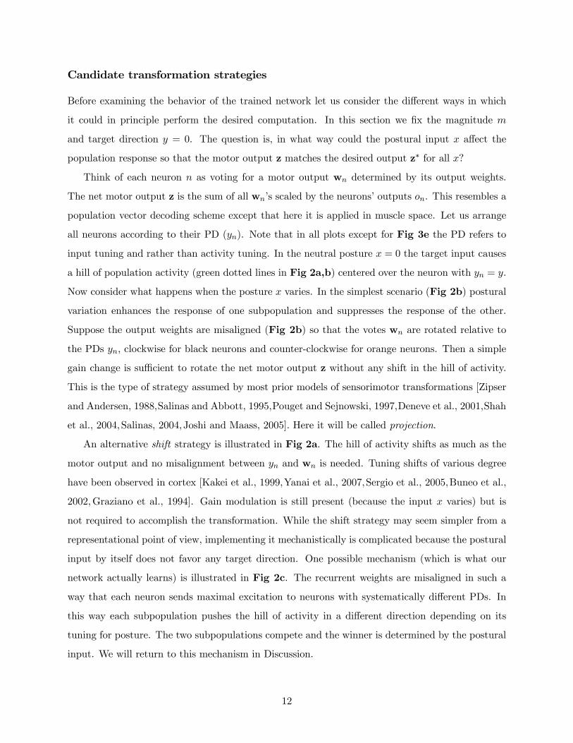
Candidate transformation strategies

Before examining the behavior of the trained network let us consider the different ways in which

it could in principle perform the desired computation. In this section we fix the magnitude m

and target direction y = 0. The question is, in what way could the postural input x affect the

population response so that the motor output z matches the desired output z∗ for all x?

Think of each neuron n as voting for a motor output wn determined by its output weights.

The net motor output z is the sum of all wn’s scaled by the neurons’ outputs on. This resembles a

population vector decoding scheme except that here it is applied in muscle space. Let us arrange

all neurons according to their PD (yn). Note that in all plots except for Fig 3e the PD refers to

input tuning and rather than activity tuning. In the neutral posture x = 0 the target input causes

a hill of population activity (green dotted lines in Fig 2a,b) centered over the neuron with yn = y.

Now consider what happens when the posture x varies. In the simplest scenario (Fig 2b) postural

variation enhances the response of one subpopulation and suppresses the response of the other.

Suppose the output weights are misaligned (Fig 2b) so that the votes wn are rotated relative to

the PDs yn, clockwise for black neurons and counter-clockwise for orange neurons. Then a simple

gain change is sufficient to rotate the net motor output z without any shift in the hill of activity.

This is the type of strategy assumed by most prior models of sensorimotor transformations [Zipser

and Andersen, 1988,Salinas and Abbott, 1995,Pouget and Sejnowski, 1997,Deneve et al., 2001,Shah

et al., 2004,Salinas, 2004,Joshi and Maass, 2005]. Here it will be called projection.

An alternative shift strategy is illustrated in Fig 2a. The hill of activity shifts as much as the

motor output and no misalignment between yn and wn is needed. Tuning shifts of various degree

have been observed in cortex [Kakei et al., 1999,Yanai et al., 2007,Sergio et al., 2005,Buneo et al.,

2002,Graziano et al., 1994]. Gain modulation is still present (because the input x varies) but is

not required to accomplish the transformation. While the shift strategy may seem simpler from a

representational point of view, implementing it mechanistically is complicated because the postural

input by itself does not favor any target direction. One possible mechanism (which is what our

network actually learns) is illustrated in Fig 2c. The recurrent weights are misaligned in such a

way that each neuron sends maximal excitation to neurons with systematically different PDs. In

this way each subpopulation pushes the hill of activity in a different direction depending on its

tuning for posture. The two subpopulations compete and the winner is determined by the postural

input. We will return to this mechanism in Discussion.

12

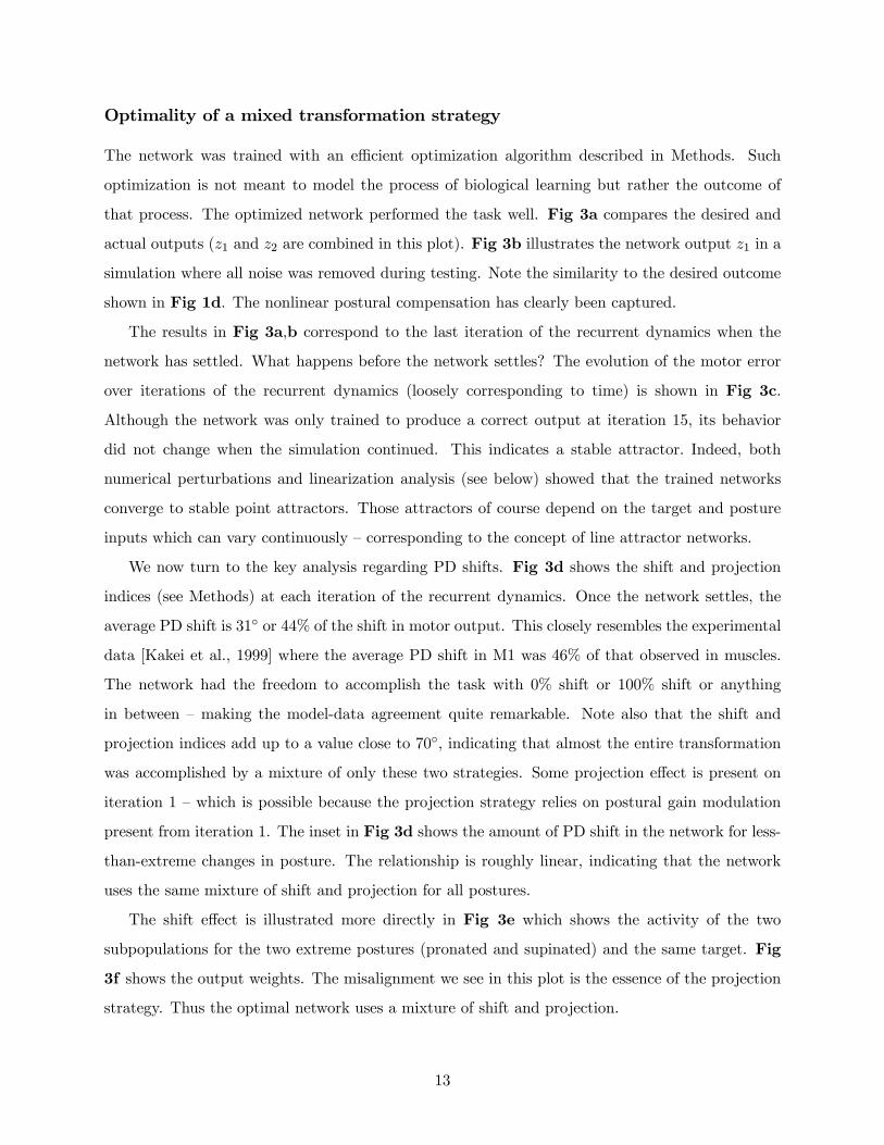
Optimality of a mixed transformation strategy

The network was trained with an efficient optimization algorithm described in Methods. Such

optimization is not meant to model the process of biological learning but rather the outcome of

that process. The optimized network performed the task well. Fig 3a compares the desired and

actual outputs (z1 and z2 are combined in this plot). Fig 3b illustrates the network output z1 in a

simulation where all noise was removed during testing. Note the similarity to the desired outcome

shown in Fig 1d. The nonlinear postural compensation has clearly been captured.

The results in Fig 3a,b correspond to the last iteration of the recurrent dynamics when the

network has settled. What happens before the network settles? The evolution of the motor error

over iterations of the recurrent dynamics (loosely corresponding to time) is shown in Fig 3c.

Although the network was only trained to produce a correct output at iteration 15, its behavior

did not change when the simulation continued. This indicates a stable attractor. Indeed, both

numerical perturbations and linearization analysis (see below) showed that the trained networks

converge to stable point attractors. Those attractors of course depend on the target and posture

inputs which can vary continuously — corresponding to the concept of line attractor networks.

We now turn to the key analysis regarding PD shifts. Fig 3d shows the shift and projection

indices (see Methods) at each iteration of the recurrent dynamics. Once the network settles, the

average PD shift is 31◦ or 44% of the shift in motor output. This closely resembles the experimental

data [Kakei et al., 1999] where the average PD shift in M1 was 46% of that observed in muscles.

The network had the freedom to accomplish the task with 0% shift or 100% shift or anything

in between — making the model-data agreement quite remarkable. Note also that the shift and

projection indices add up to a value close to 70◦, indicating that almost the entire transformation

was accomplished by a mixture of only these two strategies. Some projection effect is present on

iteration 1 — which is possible because the projection strategy relies on postural gain modulation

present from iteration 1. The inset in Fig 3d shows the amount of PD shift in the network for less-

than-extreme changes in posture. The relationship is roughly linear, indicating that the network

uses the same mixture of shift and projection for all postures.

The shift effect is illustrated more directly in Fig 3e which shows the activity of the two

subpopulations for the two extreme postures (pronated and supinated) and the same target. Fig

3f shows the output weights. The misalignment we see in this plot is the essence of the projection

strategy. Thus the optimal network uses a mixture of shift and projection.

13

Sensitivity analysis

Does the solution we found correspond to the global minimum? Three lines of evidence suggest a

positive answer. First, training was repeated many times with different initial weights. Although

every trained network was unique in its detail, the shift and projection indices were similar — see

standard deviations in Fig 4c,d. Second, in some simulations (Fig 5) certain model parameters

were varied continuously and the outcome changed smoothly. Such regularity would be unlikely

if the solutions corresponded to spurious local minima. Finally, we performed an additional set

of simulations where the network was forced to use a specified amount of shift for the first 150

iterations of gradient descent. This forcing was implemented via additional terms in the cost

function. After the first 150 iterations the extra cost terms were removed and the network was

allowed to solve the original problem. Regardless of the initial forcing the network quickly learned

the same mixture of strategies as the nominal network (Fig 4a,b), indicating a global minimum.

How does the global minimum depend on model parameters? To address this question we

trained 20 networks in each of 11 conditions, which differed from the nominal model as follows:

(1) The number of recurrent iterations was increased from 15 to 30. (2) The number of neurons

was increased from 20 to 40. (3) All noise magnitudes were reduced from 0.2 to 0.1. (4) All

noise magnitudes were increased from 0.2 to 0.4. (5) The strength of synaptic depression was

decreased from 0.1 to 0.05. (6) The strength of synaptic depression was increased from 0.1 to 0.2.

(7) All signal-dependent noise terms were replaced with additive Gaussian noise whose magnitude

matched the nominal network. (8) Instead of having two discrete subpopulations, with postural

input gradients xn either −1 or +1, here xn were sampled uniformly between −1 and +1. (9)

Another auxiliary input ex ∈ [−1,+1] was added. Its effect on the desired motor output was anonlinear scaling by a factor of 2x. The shift and projection indices were still computed with

respect to the posture x. (10) The external inputs were centered at 0 instead of being positive,

and the input noise was additive instead of being signal-dependent. (11) The conjugate gradient

descent algorithm described in Methods was replaced with the BFGS quasi-Newton algorithm as

implemented in the Matlab optimization toolbox (function "fminunc").

The shift (Fig 4c) and projection (Fig 4d) indices of the top 10 networks in each of the 11 condi-

tions were computed. Although there were some variations among conditions, the optimal solution

always involved comparable amounts of shift and projection and neither index ever approached 0.

These results indicate a general lack of sensitivity to model parameters.

14

Noise determines which transformation strategy is optimal

There was one feature of the model which greatly affected the results — namely the noise. We

already knew this from preliminary attempts to model the mixed M1 representation using deter-

ministic networks. These attempts failed in the following ways: (1) the PD half-shift observed

experimentally was never predicted by the model; (2) learning converged to multiple local minima

which did not appear to have common structure; (3) the trained networks were unstable: if we

trained them to produce a correct output on a given iteration, they produced the correct output

on that iteration but diverged immediately afterwards. This initial failure prompted us to switch

to the stochastic networks described here. Once we made the transition all of the above problems

vanished, indicating that noise makes a qualitative difference.

How can these preliminary observations be reconciled with the finding that increasing or de-

creasing all noise magnitudes by a factor of 2 has negligible effects (conditions 3 and 4 in Fig 4c,d)?

Our hypothesis was that what matters is not so much the noise magnitude, but rather the presence

or absence of different noise terms. To explore this idea quantitatively we performed another set of

sensitivity analyses focusing on the effects of noise. Fig 4e,f show seven curves each, corresponding

to varying all three noise magnitudes¡υC , υF , υI

¢together, or varying any two, or any one. The

noise magnitudes that were not varied remained fixed to their nominal value of 20%. Those that

varied were set to 0, 1, 5, 10, 30, 40, 50%. As we expected, there were abrupt changes in the shift

and projection indices between 0% and 1% noise, and little further change all the way up to 50%.

Removing all three noise terms, or the constant and fluctuating input noise terms, leads to an

optimal solution which no longer uses the shift strategy (projection is also reduced substantially).

The network still solves the problem — very accurately in fact, because noise is removed — but uses

strategies which no longer fit in our taxonomy. Removing the constant and intrinsic noise terms,

or the fluctuating and intrinsic ones, yields another interesting effect. Although the corresponding

shift and projection indices seem normal, these networks were the only ones that did not reach a

stable attractor by iteration 15. Instead their neuronal activities continued to change indefinitely.

In summary, removing any two or all three noise terms changed the outcome qualitatively, albeit

in different ways, while removing any one noise term made little difference. As long as a given noise

term was present, its exact magnitude had little effect on the shift and projection indices.

15

Noise affects multiple network properties

Since noise turned out to be the key determinant of which transformation strategy is optimal,

one would expect it to affect other network properties as well. Here we analyze these effects by

comparing training conditions in which all three noise terms were varied together (corresponding

to the thick gray lines in Fig 4e,f).

Fig 5a shows how the networks trained at every noise level performed when tested at every

other noise level. In each testing condition (row) we subtracted the minimal motor error achieved

by any network. The minima (marked with stars) are close to the diagonal, meaning that in order to

achieve optimal performance at a certain noise level the network should be trained at a similar noise

level. This finding has somewhat different flavor from our earlier finding that shift and projection

are insensitive to the exact amount of noise. The vertical rectangle in Fig 5a encloses large errors

which had to be scaled by a factor of 0.00002 to fit in our color scheme. The 0% network (i.e.

the network trained with 0% noise) performed better than any other network when tested with

0% noise, but as soon as the noise level in testing increased to even 1%, performance broke down.

The 0% network also had a very different pattern of recurrent weights when compared to all other

networks. Fig 5b shows the average recurrent weights in the best 10 networks trained in the 0%

and 1% conditions, plotted as a function of PD difference between neurons. The 1% networks (as

well as all other networks trained with noise) exhibited a clear pattern while the 0% networks did

not seem to have any common structure. This does not mean that the recurrent weights were

unimportant; on the contrary, when we tested the 0% networks with their recurrent weights either

reshuffled or set to 0, performance broke down even in the absence of noise.

The recurrent weight patterns are further analyzed in Fig 5c. We correlated the weight patterns

of each pair of networks trained in a given condition. The average R2 value (red line) was almost

zero for the 0% network, confirming that in the absence of noise different training runs converge

to solutions which lack common structure. Higher amounts of noise during training caused more

similar solutions to be found on different training runs. We also performed linear stability analysis

around the attractor states into which the recurrent dynamics settled. Ignoring the noise terms for

clarity, the recurrent dynamics can be expressed in vector notation as h (t+ 1) =WRo (h (t)) + i,

where i is the vector of external inputs, h (t) is the net input to the neurons at iteration t, o is

the transfer function and WR is the matrix of recurrent weights. The network is locally stable if

all eigenvalues of the matrix WR ∂o

∂hare smaller than 1 in absolute value. The blue line in Fig 5c

16

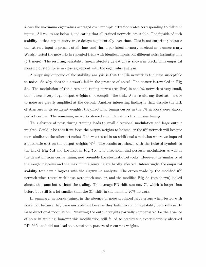
shows the maximum eigenvalues averaged over multiple attractor states corresponding to different

inputs. All values are below 1, indicating that all trained networks are stable. The flipside of such

stability is that any memory trace decays exponentially over time. This is not surprising because

the external input is present at all times and thus a persistent memory mechanism is unnecessary.

We also tested the networks in repeated trials with identical inputs but different noise instantiations

(5% noise). The resulting variability (mean absolute deviation) is shown in black. This empirical

measure of stability is in close agreement with the eigenvalue analysis.

A surprising outcome of the stability analysis is that the 0% network is the least susceptible

to noise. So why does this network fail in the presence of noise? The answer is revealed in Fig

5d. The modulation of the directional tuning curves (red line) in the 0% network is very small,

thus it needs very large output weights to accomplish the task. As a result, any fluctuations due

to noise are greatly amplified at the output. Another interesting finding is that, despite the lack

of structure in its recurrent weights, the directional tuning curves in the 0% network were almost

perfect cosines. The remaining networks showed small deviations from cosine tuning.

Thus absence of noise during training leads to small directional modulation and large output

weights. Could it be that if we force the output weights to be smaller the 0% network will become

more similar to the other networks? This was tested in an additional simulation where we imposed

a quadratic cost on the output weights WZ . The results are shown with the isolated symbols to

the left of Fig 5,d and the inset in Fig 5b. The directional and postural modulation as well as

the deviation from cosine tuning now resemble the stochastic networks. However the similarity of

the weight patterns and the maximum eigenvalue are hardly affected. Interestingly, the empirical

stability test now disagrees with the eigenvalue analysis. The errors made by the modified 0%

network when tested with noise were much smaller, and the modified Fig 5a (not shown) looked

almost the same but without the scaling. The average PD shift was now 7◦, which is larger than

before but still is a lot smaller than the 31◦ shift in the nominal 20% network.

In summary, networks trained in the absence of noise produced large errors when tested with

noise, not because they were unstable but because they failed to combine stability with sufficiently

large directional modulation. Penalizing the output weights partially compensated for the absence

of noise in training, however this modification still failed to predict the experimentally observed

PD shifts and did not lead to a consistent pattern of recurrent weights.

17

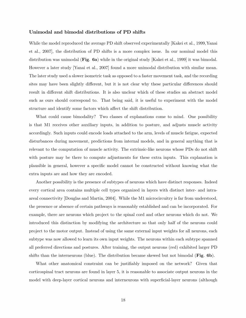
Unimodal and bimodal distributions of PD shifts

While the model reproduced the average PD shift observed experimentally [Kakei et al., 1999,Yanai

et al., 2007], the distribution of PD shifts is a more complex issue. In our nominal model this

distribution was unimodal (Fig. 6a) while in the original study [Kakei et al., 1999] it was bimodal.

However a later study [Yanai et al., 2007] found a more unimodal distribution with similar mean.

The later study used a slower isometric task as opposed to a faster movement task, and the recording

sites may have been slightly different, but it is not clear why these particular differences should

result in different shift distributions. It is also unclear which of these studies an abstract model

such as ours should correspond to. That being said, it is useful to experiment with the model

structure and identify some factors which affect the shift distribution.

What could cause bimodality? Two classes of explanations come to mind. One possibility

is that M1 receives other auxiliary inputs, in addition to posture, and adjusts muscle activity

accordingly. Such inputs could encode loads attached to the arm, levels of muscle fatigue, expected

disturbances during movement, predictions from internal models, and in general anything that is

relevant to the computation of muscle activity. The extrinsic-like neurons whose PDs do not shift

with posture may be there to compute adjustments for these extra inputs. This explanation is

plausible in general, however a specific model cannot be constructed without knowing what the

extra inputs are and how they are encoded.

Another possibility is the presence of subtypes of neurons which have distinct responses. Indeed

every cortical area contains multiple cell types organized in layers with distinct inter- and intra-

areal connectivity [Douglas and Martin, 2004]. While the M1 microcircuitry is far from understood,

the presence or absence of certain pathways is reasonably established and can be incorporated. For

example, there are neurons which project to the spinal cord and other neurons which do not. We

introduced this distinction by modifying the architecture so that only half of the neurons could

project to the motor output. Instead of using the same external input weights for all neurons, each

subtype was now allowed to learn its own input weights. The neurons within each subtype spanned

all preferred directions and postures. After training, the output neurons (red) exhibited larger PD

shifts than the interneurons (blue). The distribution became skewed but not bimodal (Fig. 6b).

What other anatomical constraint can be justifiably imposed on the network? Given that

corticospinal tract neurons are found in layer 5, it is reasonable to associate output neurons in the

model with deep-layer cortical neurons and interneurons with superficial-layer neurons (although

18

a caudal-rostral distinction is also plausible). Canonical microcircuit models [Douglas and Martin,

2004] suggest that superficial and deep layers (3 and 5 in particular) are fully interconnected, but

this is mostly based on data from sensory cortices. Motor cortex has the interesting feature that

deep-layer pyramidal neurons do not appear to project to the superficial layers [Ghosh and Porter,

1988]. This was incorporated in a further modification where the projection from output neurons to

interneurons was removed. Thus interneurons could project to themselves and to output neurons,

while output neurons could project to themselves and to muscles. The distribution of PD shifts after

training was now clearly bimodal (Fig. 6c). Despite the large difference in directional tuning, the

two subpopulations exhibited comparable amounts of postural gain modulation. This was tested by

defining a gain-modulation index as the absolute difference between firing rates in the two extreme

postures divided by the neuron’s overall firing rate. The shift index accounted for less than 5% of

the variance of this gain-modulation index in all models. We also applied this analysis to the raw

M1 data kindly provided by Kakei et al. As in the model, PD shifts in M1 accounted for less than

5% of the variance in the gain-modulation index.

A complication with subpopulation modeling is that on one hand output neurons are a minority,

while on the other hand M1 recordings are biased towards them. Another complication is that not

all output neurons project to the spinal cord, raising the possibility of further subdivision. For

example, layer 5 M1 neurons projecting to the striatum have more extrinsic-like responses that

corticospinal neurons [Turner and DeLong, 2000]. A model cannot be expected to fully resolve

these issues without additional data. To remain agnostic, the present subpopulation model assumed

equal numbers of interneurons and output neurons.

19

Discussion

We presented a recurrent neural network model of M1 which transforms reach targets and arm

postures into muscle activations. When trained in the presence of noise, the network reproduced

the mixed muscle-movement representation observed experimentally [Kakei et al., 1999,Yanai et al.,

2007]. Thus, even if M1 is a muscle controller, its activity would be more extrinsic-like than

muscle activity because such a representation reflects the optimal way to perform the sensorimotor

transformation. Our work provides a rare example of resolving redundancy on the neural level —

by showing not only that a given network mechanism fits data, but furthermore that the brain has

good reasons to select this particular mechanism over all alternatives.

We did not explain why noise has the effects it has on the optimal solution, and indeed at this

point we do not have a satisfying explanation. Ideally we would derive a formula showing how the

optimal solution depends on model parameters. However there are no available mathematical tools

that could yield such results for nonlinear stochastic dynamics. Instead we provided extensive sim-

ulations which illustrated the effects of noise on multiple network properties. All existing neuronal

models (including ours) are likely to underestimate the true diversity of noise sources in the brain.

Thus the fact that increasing noise diversity leads to better model-data agreement is encouraging.

Although we focused on one sensorimotor transformation, our model may reflect the general role

that M1 plays in movement production. We believe M1’s role is to translate goal-related signals into

muscle activations while compensating for the state of the musculo-skeletal apparatus. In everyday

tasks involving many degrees of freedom (especially hand manipulation), such compensation is

likely to be a very challenging computational problem which requires an entire cortical area. The

postural rotation studied here is a good start but it does not do justice to this general problem.

Further progress would require data from more complex tasks performed in multiple postures.

On the role of the spinal cord

As in our previous work [Todorov, 2000,Todorov, 2003], here we assumed that the M1 population

output is related to the pattern of muscle activity through a linear mapping. This is an approxima-

tion to the combined effect of direct corticomotoneuronal projections and indirect pathways through

spinal interneurons. Linearity is not a particularly restrictive assumption because any smooth map-

ping can be locally approximated as being linear. Our assumption however has a deeper implication

— which is that muscle activity is determined by the descending drive and does not depend on ad-

20

ditional signals available to the spinal cord. This cannot be true in general, because the spinal cord

acts as a fast feedback controller and uses proprioceptive information to modulate muscle activity

before cortex has received that information. Such a low-level sensorimotor loop can be very useful

for counteracting unexpected disturbances. Anything that is expected, however, is more likely to

be incorporated in the descending drive. In the unperturbed and overtrained movements studied

in the M1 literature unexpected disturbances are negligible — which may be the reason why our

models can do such a good job explaining M1 data while ignoring the spinal cord. A further reason

is that here we focused on movement initiation where spinal feedback is unlikely to play a role.

One possible criticism of the model is that we asked our network to perform the entire trans-

formation from extrinsic to muscle space. What if M1 performs only part of the transformation

and the circuits in the spinal cord perform the remaining part? While this is in principle possible,

recent recordings in the spinal cord [Yanai et al., 2007] contradict this hypothesis and show that

even the earliest directionally-tuned activity of spinal interneurons is muscle-like.

Modeling additional sensorimotor transformations

The M1 datasets [Kakei et al., 1999,Yanai et al., 2007] are not the only known examples of mixed

representations. In parietal area 5, the representation of reach targets was found to be neither

eye-centered nor hand-centered but somewhere in between — suggesting a "direct visuomotor trans-

formation" [Buneo et al., 2002]. In that case the half-shift effect was observed in positional tuning

curves rather than directional tuning curves, and the auxiliary input was hand position rather than

forearm orientation. An extension of our model to this dataset should be straightforward. The

model could also be extended to a more complex setting where monkeys made reaching movements

while their arm was in the natural versus abducted posture [Scott and Kalaska, 1997]. Posture

affected both the mean firing rates and preferred directions of M1 neurons. A specific model of

this experiment would require a 4-degree-of-freedom arm with a substantial number of muscles

whose pulling directions have realistic dependence on posture. Once such a biomechanical model is

available, the methods developed here should be directly applicable although training the network

will probably be slower.

Another well-known postural effect in M1 is the horizontal PD shift caused by rotating the

workspace around the shoulder [Caminiti et al., 1991,Sergio et al., 2005]. However that phenomenon

may have a different origin. Horizontal hand-target vectors are likely to be encoded in an intrinsic

frame even in higher-level areas because such a frame better reflects the properties of the sensory

21

periphery (radial distance to a fixated object is extracted from visual depth cues while azimuth and

elevation are extracted from extraretinal signals). More generally, we suspect that 3D hand-target

vectors in premotor as well as parietal cortex are represented in a cylindrical frame, where "down"

is towards the feet, "forward" is away from the body, and "left-right" is around the body. If such

a 3D frame is examined in different 2D sections, the horizontal (transversal) section will appear

intrinsic while the vertical (sagittal and coronal) sections will appear extrinsic.

Mechanisms for shifting tuning curves

Apart from the illustration in Fig 2c, we did not discuss the recurrent mechanisms which al-

lowed the network to shift its hill of activity in response to a diffuse postural signal. We have

performed extensive analysis of these mechanisms which will be presented elsewhere. Briefly, when

the between- and within-subpopulation recurrent weights follow cosine patterns, networks with

arbitrary numbers of neurons can be reduced to nonlinear dynamical systems with only 6 state

variables. This is because the hill of activity over each subpopulation is a cosine, and a cosine

can be described by three variables (phase, offset, gain). Such analysis clarifies the deterministic

aspects of the network, however we found that it does not shed light on the effects of noise. When

we projected the noise and optimized the low-dimensional model, the solution did not correspond

well to the optimal solution in the full model. This, along with the considerable length of the

manuscript, is the reason for leaving the analysis of network mechanisms for another paper.

Shifting of tuning curves under the influence of auxiliary or contextual signals is a general

problem which has been studied in computational neuroscience [Droulez and Berthoz, 1991,Zhang,

1996,Burnod et al., 1992,Zhang and Abbott, 2000,Hahnloser et al., 1999,Deneve et al., 2001]. While

a detailed comparison to these prior models will be given elsewhere, here we make a couple of points

relevant to the present study. Prior models of shifting require neuronal interactions which are more

complex than the additive synapses we used. Some models [Droulez and Berthoz, 1991, Zhang,

1996,Burnod et al., 1992,Zhang and Abbott, 2000] rely on multiplicative synapses. Others assume

that all recurrent interactions are channeled through a few specialized "pointer" neurons [Hahnloser

et al., 1999, Zhang and Abbott, 2000], or that the network performs divisive normalization via

unspecified synaptic interactions [Deneve et al., 2001]. Another important difference here is that

we addressed the issue of optimality (in particular optimality under noise), and constructed our

networks through learning instead of manually.

22

References

[Allen and Stevens, 1994] Allen, C. and Stevens, C. (1994). An evaluation of causes for unreliability

of synaptic transmission. Proc Natl Acad Sci, 91:10380—10383.

[Bernstein, 1967] Bernstein, N. (1967). The Coordination and Regulation of Movements. Pergamon

Press.

[Buneo et al., 2002] Buneo, C., Jarvis, M., Batista, A., and Andersen, R. (2002). Direct visuomotor

transformations for reaching. Nature, 416:632—636.

[Burnod et al., 1992] Burnod, Y., Grandguillaume, P., Ferraina, S., Johnson, P., and Caminiti, R.

(1992). Visuomotor tranformations underlying arm movements toward visual targets: a neural

network model of cerebral cortical operations. J.Neuroscience, 12(4):1435—1453.

[Caminiti et al., 1991] Caminiti, R., Johnson, P., Galli, C., Ferraina, S., and Burnod, Y. (1991).

Making arm movements within different parts of space: The premotor and motor cortical repre-

sentation of a coordinate system for reaching to visual targets. J Neurosci, 11(5):1182—97.

[Deneve et al., 2001] Deneve, S., Latham, P., and Pouget, A. (2001). Efficient computation and

cue integration with noisy population codes. Nat.Neurosci., 4(8):826—831.

[Douglas and Martin, 2004] Douglas, R. and Martin, K. (2004). Neuronal circuits of the neocortex.

Annu Rev Neurosci, 27:419—451.

[Droulez and Berthoz, 1991] Droulez, J. and Berthoz, A. (1991). A neural network model of sensori-

topic maps with predictive short-term memory properties. Proc. Natl. Acad. Sci., 88:9653—9657.

[Evarts, 1981] Evarts, E. (1981). Role of motor cortex in voluntary movements in primates. In

Brooks, V., editor, Handbook of Physiology, volume 2, pages 1083—1120. Williams and Wilkins,

Baltimore.

[Fetz, 1992] Fetz, E. (1992). Are movement parameters recognizably coded in the activity of single

neurons? Behav Brain Sci, 15:679—690.

[Georgopoulos et al., 1983] Georgopoulos, A., Caminiti, R., Kalaska, J., and Massey, J. (1983).

Spatial coding of movement: a hypothesis concerning the coding of movement direction by motor

cortical populations. Experimental Brain Research, Supplement 7:327—336.

23

[Georgopoulos et al., 1982] Georgopoulos, A., Kalaska, J., Caminiti, R., and Massey, J. (1982).

On the relations between the direction of two-dimensional arm movements and cell discharge in

primate motor cortex. J.Neurosci., 2(11):1527—1537.

[Ghosh and Porter, 1988] Ghosh, S. and Porter, R. (1988). Morphology of pyramidal neurones in

monkey motor cortex and the synaptic actions of their intracortical axon collaterals. Journal of

Physiology, 400:593—615.

[Graziano et al., 1994] Graziano, M., Yap, G., and Gross, C. (1994). Coding of visual space by

premotor neurons. Science, 266:1054—1057.

[Hahnloser et al., 1999] Hahnloser, R., Douglas, R., Mahowald, M., and Hepp, K. (1999). Feedback

interactions between neuronal pointers and maps for attentional processing. Nat Neurosci, 2:746—

752.

[Harris and Wolpert, 1998] Harris, C. and Wolpert, D. (1998). Signal-dependent noise determines

motor planning. Nature, 394:780—784.

[Hertz et al., 1991] Hertz, J., Krogh, A., and Palmer, R. (1991). Introduction to the Theory of

Neural Computation. Addison-Wesley, Redwood City, CA.

[Hessler et al., 1993] Hessler, N., Shirke, A., and Malinow, R. (1993). The probability of transmitter

release at a mammalian central synapse. Nature, 366:569—572.

[Joshi and Maass, 2005] Joshi, P. and Maass, W. (2005). Movement generation with networks of

spiking neurons. Neural computation, 17:1715—1738.

[Kakei et al., 1999] Kakei, S., Hoffman, D., and Strick, P. (1999). Muscle and movement represen-

tations in the primary motor cortex. Science, 285:2136—2139.

[Kakei et al., 2001] Kakei, S., Hoffman, D., and Strick, P. (2001). Direction of action is represented

in the ventral premotor cortex. Nat.Neurosci., 4(10):1020—1025.

[Kakei et al., 2003] Kakei, S., Hoffman, D., and Strick, P. (2003). Sensorimotor transformations in

cortical motor areas. Neuroscience Research, 46:1—10.

[Kettner et al., 1988] Kettner, R. E., Schwartz, A. B., and Georgopoulos, A. P. (1988). Primate

motor cortex and free arm movements to visual targets in three-dimensional space. J Neurosci,

8(8):2938—2947.

24

[Krutzer et al., 2007] Krutzer, I., Herter, T., Georgopoulos, A., Naseralis, T., Merchant, H., and

Amirikian, B. (2007). Contrasting interpretations of the nonunifrm distribution of preferred

directions within primary motor cortex. Journal of Neurophysiology, 97:4390—4392.

[Moran et al., 2000] Moran, D., Schwartz, A., Georgopoulos, A., Ashe, J., Todorov, E., and Scott,

S. (2000). One motor cortex, two different views. Nature Neuroscience, 3(10):963—965.

[Ng and Jordan, 2000] Ng, A. and Jordan, M. (2000). Pegasus: A policy search method for large

mdps and pomdps. Uncertainty in artificial intelligence, 16.

[Pouget and Sejnowski, 1997] Pouget, A. and Sejnowski, T. (1997). Spatial transformation in the

parietal cortex using basis functions. J Cogn Neurosci, 9:222—237.

[Press et al., 1986] Press, W., Flannery, B., Teukolsky, S., and Vetterling, W. (1986). Numerical

recipes in C. Cambridge University Press, Cambrdige, MA.

[Salinas, 2004] Salinas, E. (2004). Fast remapping of sensory stimuli onto motor actions on the

basis of contextual modulation. J Neurosci, 24:1113—1118.

[Salinas and Abbott, 1995] Salinas, E. and Abbott, L. (1995). Transfer of coded information from

sensory to motor networks. J Neurosci, 15:6461—6467.

[Scholz and Schoner, 1999] Scholz, J. and Schoner, G. (1999). The uncontrolled manifold concept:

identifying control variables for a functional task. Exp Brain Res, 126(3):289—306.

[Scott and Kalaska, 1997] Scott, S. and Kalaska, J. (1997). Reaching movements with similar hand

paths but different arm orientation. J Neurophys, 77:826—852.

[Sergio et al., 2005] Sergio, L., Hamel-Paquet, C., and Kalaska, J. (2005). Motor cortex neural cor-

relates of output kinematics and kinetics during isometric-force and arm-reaching tasks. Journal

of Neurophysiology, 94:2353—2378.

[Shah et al., 2004] Shah, A., Fagg, A., and Barto, A. (2004). Cortical involvement in the recruit-

ment of wrist muscles. J Neurophys, 91:2445—2456.

[Todorov, 2000] Todorov, E. (2000). Direct cortical control of muscle activation in voluntary arm

movements: a model. Nature Neuroscience, 3(4):391—398.

25

[Todorov, 2002] Todorov, E. (2002). Cosine tuning minimizes motor errors. Neural Computation,

14(6):1233—1260.

[Todorov, 2003] Todorov, E. (2003). On the role of primary motor cortex in arm movement control.

In Latash, M. and Levin, M., editors, Progress in Motor Control III, pages 125—166. Human

Kinetics.

[Todorov, 2004] Todorov, E. (2004). Optimality principles in sensorimotor control. Nature Neuro-

science, 7(9):907—915.

[Todorov and Jordan, 2002] Todorov, E. and Jordan, M. (2002). Optimal feedback control as a

theory of motor coordination. Nature Neuroscience, 5(11):1226—1235.

[Tsodyks and Markram, 1997] Tsodyks, M. and Markram, H. (1997). The neural code between

neocortical pyramidal neurons depends on neurotransmitter release probability. Proc Natl Acad

Sci, 94:719—723.

[Turner and DeLong, 2000] Turner, R. and DeLong, M. (2000). Corticostriatal activity in primary

motor cortex of the macaque. Journal of Neuroscience, 20:7096—7108.

[Yanai et al., 2007] Yanai, Y., Adamit, N. Israel, Z., Harel, R., and Prut, Y. (2007). Coordinate

transformation is first completed downstream of primary motor cortex. Journal of Neuroscience,

28:1728—1732.

[Zhang and Abbott, 2000] Zhang, J. and Abbott, L. (2000). Gain modulation of recurrent net-

works. Neurocomputing, 32-33:623—628.

[Zhang, 1996] Zhang, K. (1996). Representation of spatial orientation by the intrinsic dynamics of

the head-direction cell ensemble: A theory. J Neurosci, 16:2112—2126.

[Zipser and Andersen, 1988] Zipser, D. and Andersen, R. (1988). A back-propagation programmed

network that simulates response properties of a subset of posterior parietal neurons. Nature,

331:679—684.

26

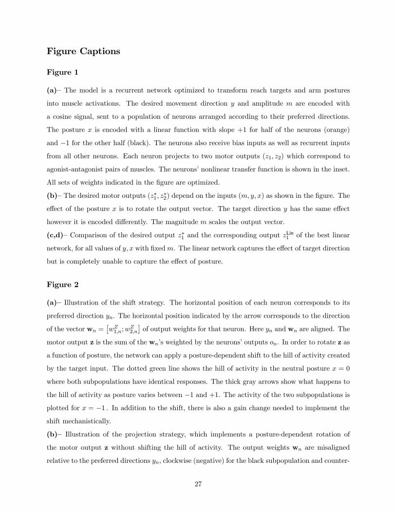
Figure Captions

Figure 1

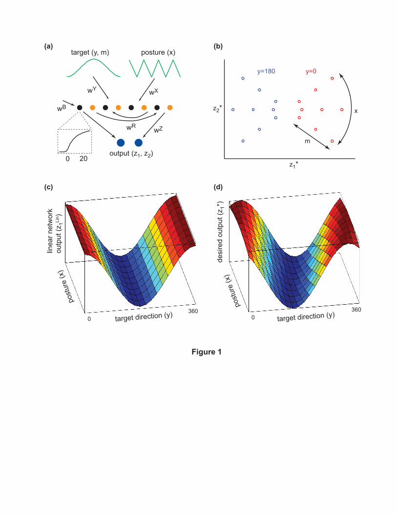
(a)— The model is a recurrent network optimized to transform reach targets and arm postures

into muscle activations. The desired movement direction y and amplitude m are encoded with

a cosine signal, sent to a population of neurons arranged according to their preferred directions.

The posture x is encoded with a linear function with slope +1 for half of the neurons (orange)

and −1 for the other half (black). The neurons also receive bias inputs as well as recurrent inputs

from all other neurons. Each neuron projects to two motor outputs (z1, z2) which correspond to

agonist-antagonist pairs of muscles. The neurons’ nonlinear transfer function is shown in the inset.

All sets of weights indicated in the figure are optimized.

(b)— The desired motor outputs (z∗1, z∗2) depend on the inputs (m, y, x) as shown in the figure. The

effect of the posture x is to rotate the output vector. The target direction y has the same effect

however it is encoded differently. The magnitude m scales the output vector.

(c,d)— Comparison of the desired output z∗1 and the corresponding output zLin1 of the best linear

network, for all values of y, x with fixedm. The linear network captures the effect of target direction

but is completely unable to capture the effect of posture.

Figure 2

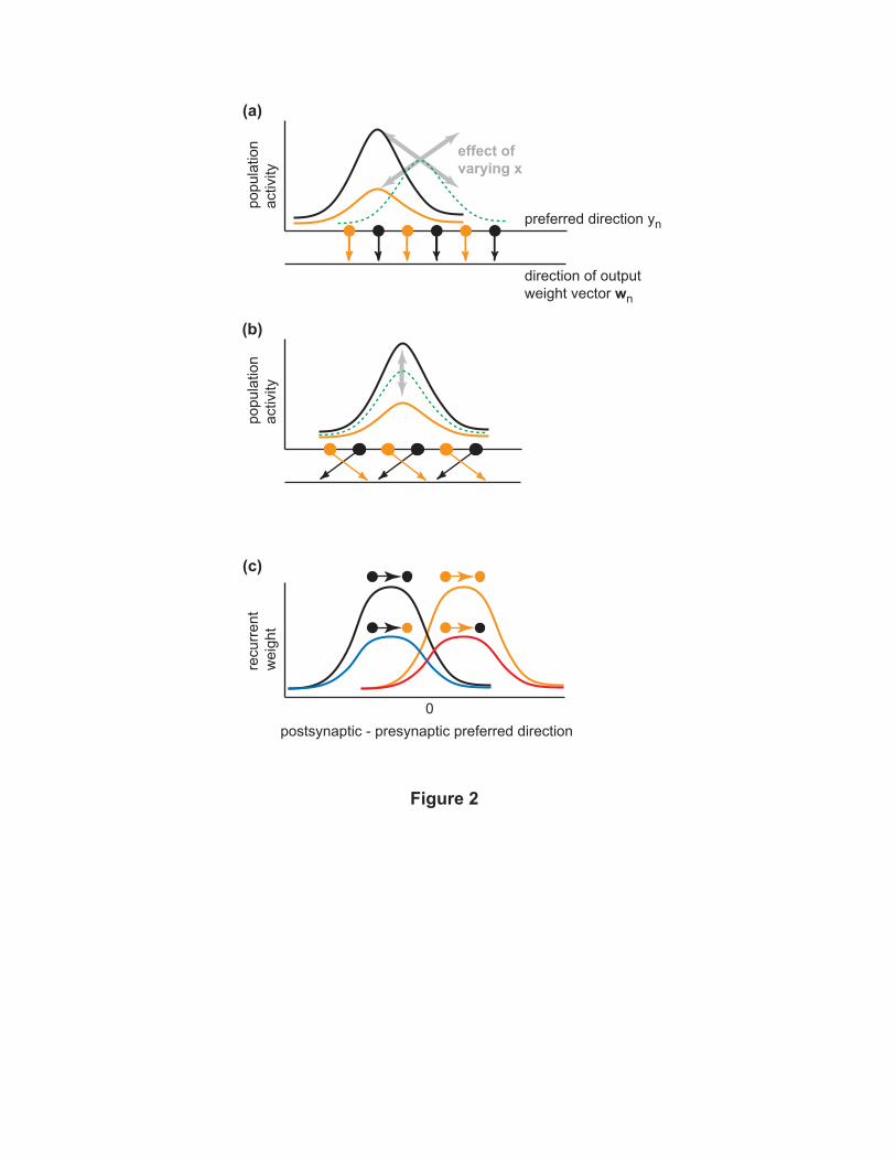
(a)— Illustration of the shift strategy. The horizontal position of each neuron corresponds to its

preferred direction yn. The horizontal position indicated by the arrow corresponds to the direction

of the vector wn =£wZ1,n;w

Z2,n

¤of output weights for that neuron. Here yn and wn are aligned. The

motor output z is the sum of the wn’s weighted by the neurons’ outputs on. In order to rotate z as

a function of posture, the network can apply a posture-dependent shift to the hill of activity created

by the target input. The dotted green line shows the hill of activity in the neutral posture x = 0

where both subpopulations have identical responses. The thick gray arrows show what happens to

the hill of activity as posture varies between −1 and +1. The activity of the two subpopulations is

plotted for x = −1 . In addition to the shift, there is also a gain change needed to implement the

shift mechanistically.

(b)— Illustration of the projection strategy, which implements a posture-dependent rotation of

the motor output z without shifting the hill of activity. The output weights wn are misaligned

relative to the preferred directions yn, clockwise (negative) for the black subpopulation and counter-

27

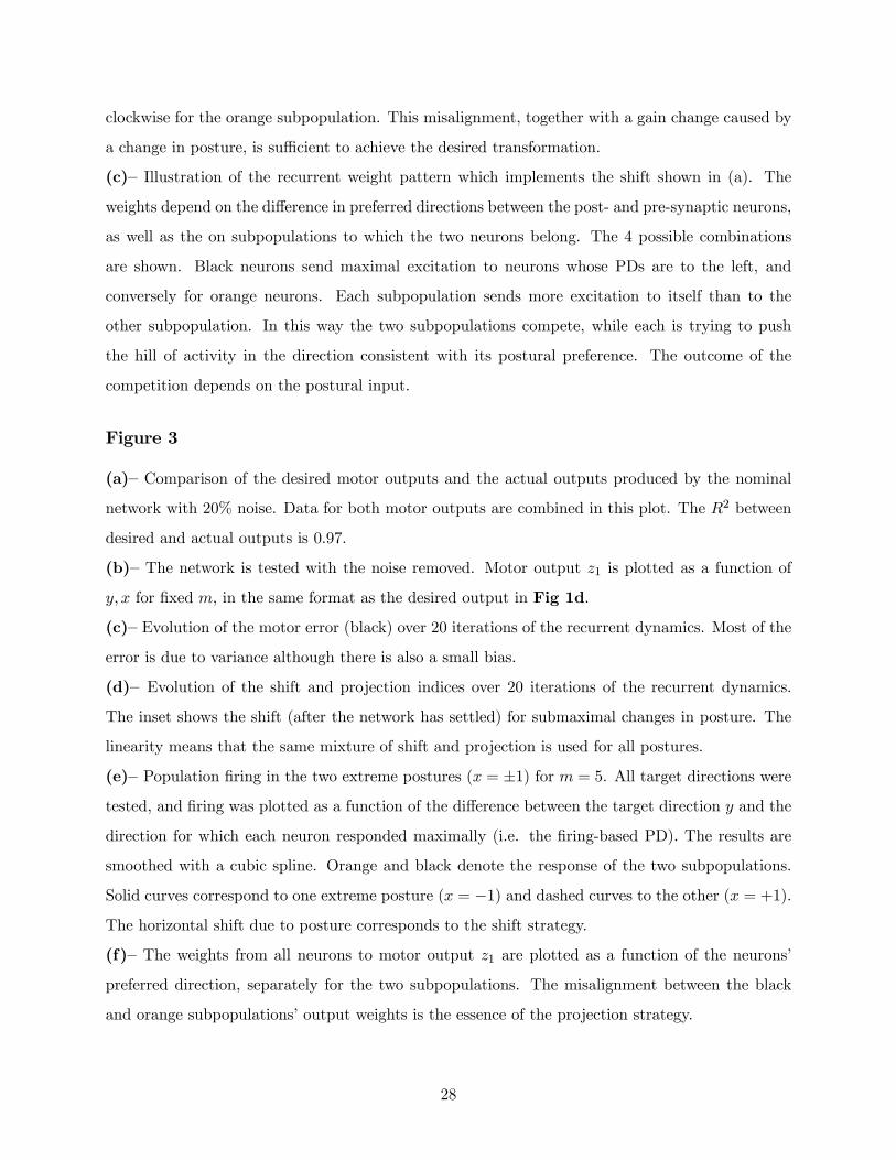
clockwise for the orange subpopulation. This misalignment, together with a gain change caused by

a change in posture, is sufficient to achieve the desired transformation.

(c)— Illustration of the recurrent weight pattern which implements the shift shown in (a). The

weights depend on the difference in preferred directions between the post- and pre-synaptic neurons,

as well as the on subpopulations to which the two neurons belong. The 4 possible combinations

are shown. Black neurons send maximal excitation to neurons whose PDs are to the left, and

conversely for orange neurons. Each subpopulation sends more excitation to itself than to the

other subpopulation. In this way the two subpopulations compete, while each is trying to push

the hill of activity in the direction consistent with its postural preference. The outcome of the

competition depends on the postural input.

Figure 3

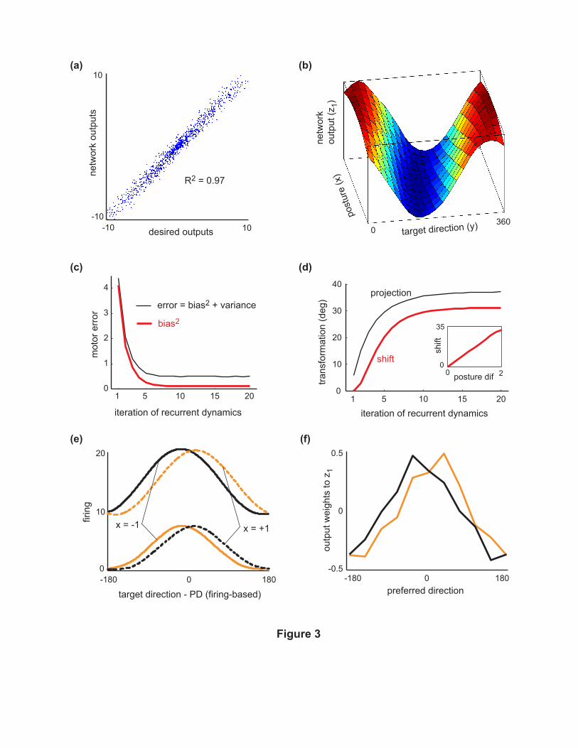
(a)— Comparison of the desired motor outputs and the actual outputs produced by the nominal

network with 20% noise. Data for both motor outputs are combined in this plot. The R2 between

desired and actual outputs is 0.97.

(b)— The network is tested with the noise removed. Motor output z1 is plotted as a function of

y, x for fixed m, in the same format as the desired output in Fig 1d.

(c)— Evolution of the motor error (black) over 20 iterations of the recurrent dynamics. Most of the

error is due to variance although there is also a small bias.

(d)— Evolution of the shift and projection indices over 20 iterations of the recurrent dynamics.

The inset shows the shift (after the network has settled) for submaximal changes in posture. The

linearity means that the same mixture of shift and projection is used for all postures.

(e)— Population firing in the two extreme postures (x = ±1) for m = 5. All target directions were

tested, and firing was plotted as a function of the difference between the target direction y and the

direction for which each neuron responded maximally (i.e. the firing-based PD). The results are

smoothed with a cubic spline. Orange and black denote the response of the two subpopulations.

Solid curves correspond to one extreme posture (x = −1) and dashed curves to the other (x = +1).

The horizontal shift due to posture corresponds to the shift strategy.

(f)— The weights from all neurons to motor output z1 are plotted as a function of the neurons’

preferred direction, separately for the two subpopulations. The misalignment between the black

and orange subpopulations’ output weights is the essence of the projection strategy.

28

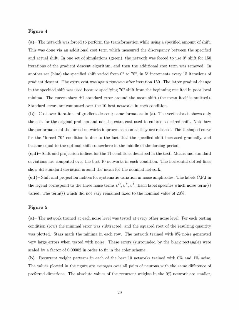
Figure 4

(a)— The network was forced to perform the transformation while using a specified amount of shift.

This was done via an additional cost term which measured the discrepancy between the specified

and actual shift. In one set of simulations (green), the network was forced to use 0◦ shift for 150

iterations of the gradient descent algorithm, and then the additional cost term was removed. In

another set (blue) the specified shift varied from 0◦ to 70◦, in 5◦ increments every 15 iterations of

gradient descent. The extra cost was again removed after iteration 150. The latter gradual change

in the specified shift was used because specifying 70◦ shift from the beginning resulted in poor local

minima. The curves show ±1 standard error around the mean shift (the mean itself is omitted).

Standard errors are computed over the 10 best networks in each condition.

(b)— Cost over iterations of gradient descent; same format as in (a). The vertical axis shows only

the cost for the original problem and not the extra cost used to enforce a desired shift. Note how

the performance of the forced networks improves as soon as they are released. The U-shaped curve

for the "forced 70" condition is due to the fact that the specified shift increased gradually, and

became equal to the optimal shift somewhere in the middle of the forcing period.

(c,d)— Shift and projection indices for the 11 conditions described in the text. Means and standard

deviations are computed over the best 10 networks in each condition. The horizontal dotted lines

show ±1 standard deviation around the mean for the nominal network.

(e,f)— Shift and projection indices for systematic variation in noise amplitudes. The labels C,F,I in

the legend correspond to the three noise terms υC , υF , υI . Each label specifies which noise term(s)

varied. The term(s) which did not vary remained fixed to the nominal value of 20%.

Figure 5

(a)— The network trained at each noise level was tested at every other noise level. For each testing

condition (row) the minimal error was subtracted, and the squared root of the resulting quantity

was plotted. Stars mark the minima in each row. The network trained with 0% noise generated

very large errors when tested with noise. These errors (surrounded by the black rectangle) were

scaled by a factor of 0.00002 in order to fit in the color scheme.

(b)— Recurrent weight patterns in each of the best 10 networks trained with 0% and 1% noise.

The values plotted in the figure are averages over all pairs of neurons with the same difference of

preferred directions. The absolute values of the recurrent weights in the 0% network are smaller,

29

but not as small as they appear in the figure. Since these weights lack a systematic pattern,

averaging over pairs of neurons makes them look smaller. The inset shows the recurrent weights

for a modified 0% network whose output weights are penalized in the cost function.

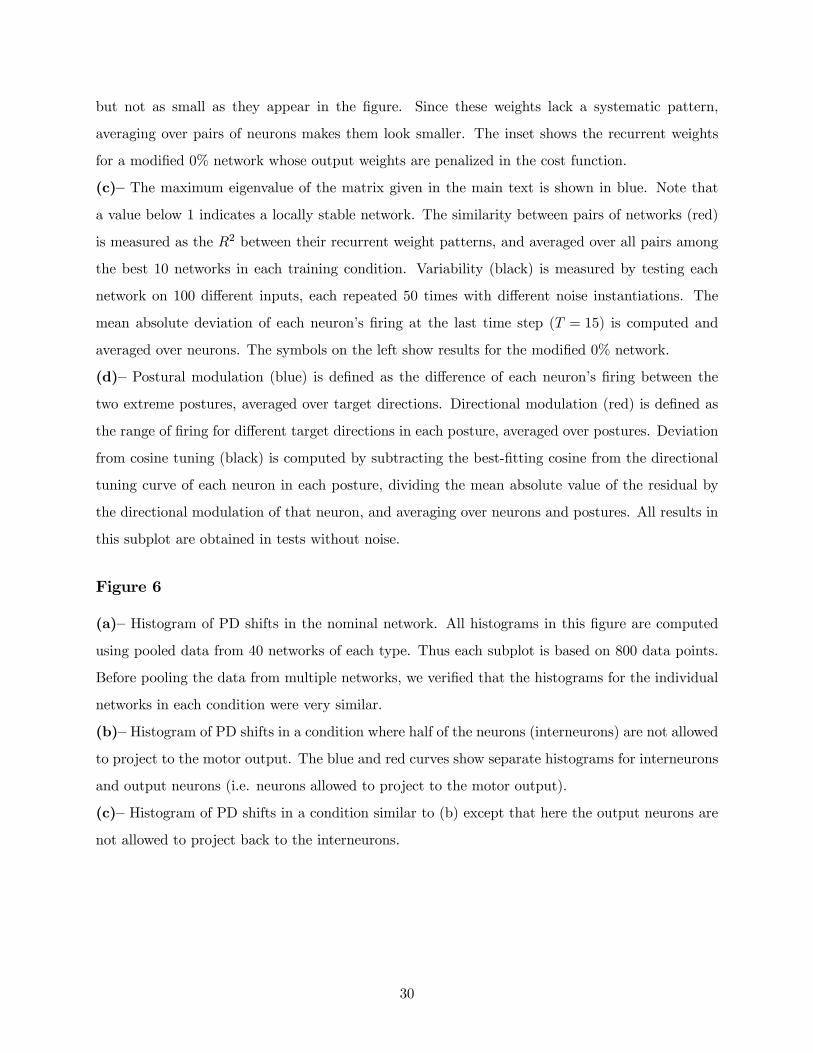
(c)— The maximum eigenvalue of the matrix given in the main text is shown in blue. Note that

a value below 1 indicates a locally stable network. The similarity between pairs of networks (red)

is measured as the R2 between their recurrent weight patterns, and averaged over all pairs among

the best 10 networks in each training condition. Variability (black) is measured by testing each

network on 100 different inputs, each repeated 50 times with different noise instantiations. The

mean absolute deviation of each neuron’s firing at the last time step (T = 15) is computed and

averaged over neurons. The symbols on the left show results for the modified 0% network.

(d)— Postural modulation (blue) is defined as the difference of each neuron’s firing between the

two extreme postures, averaged over target directions. Directional modulation (red) is defined as

the range of firing for different target directions in each posture, averaged over postures. Deviation

from cosine tuning (black) is computed by subtracting the best-fitting cosine from the directional

tuning curve of each neuron in each posture, dividing the mean absolute value of the residual by

the directional modulation of that neuron, and averaging over neurons and postures. All results in

this subplot are obtained in tests without noise.

Figure 6

(a)— Histogram of PD shifts in the nominal network. All histograms in this figure are computed

using pooled data from 40 networks of each type. Thus each subplot is based on 800 data points.

Before pooling the data from multiple networks, we verified that the histograms for the individual

networks in each condition were very similar.

(b)— Histogram of PD shifts in a condition where half of the neurons (interneurons) are not allowed

to project to the motor output. The blue and red curves show separate histograms for interneurons

and output neurons (i.e. neurons allowed to project to the motor output).

(c)— Histogram of PD shifts in a condition similar to (b) except that here the output neurons are

not allowed to project back to the interneurons.

30

wY wX

wR wZ

output (z1, z2)

wB

0 20

posture (x)target (y, m)

Figure 1

m

x

y=0y=180

z1*

z2*

(a) (b)

(d)(c)

post

ure

(x)

target direction (y)

desi

red

outp

ut (z

1*)

linea

r net

wor

kou

tput

(z1Li

n )

target direction (y)

post

ure

(x)

0360

0360

(a)

(b)

preferred direction yn

direction of outputweight vector wn

effect ofvarying x

Figure 2

(c)

postsynaptic - presynaptic preferred direction0

popu

latio

nac

tivity

popu

latio

nac

tivity

recu

rren

tw

eigh

t

(c)

iteration of recurrent dynamics

1 5 10 15 200

1

2

3

4

mot

or e

rror

error = bias2 + variance

bias2

Figure 3

target direction - PD (firing-based)

firin

g

-180 0 1800

10

20

0 20

35

posture dif

shift

1 5 10 15 200

10

20

30

40

iteration of recurrent dynamics

trans

form

atio

n (d

eg)

projection

shift

(e)

(d)

-180 0 180-0.5

0

0.5

outp

ut w

eigh

ts to

z1

(a) (b)

(f)

-10 10

10

-10

desired outputs

netw

ork

outp

uts

post

ure

(x)

target direction (y)

netw

ork

outp

ut (z

1)

x = -1 x = +1

preferred direction

0360

R2 = 0.97

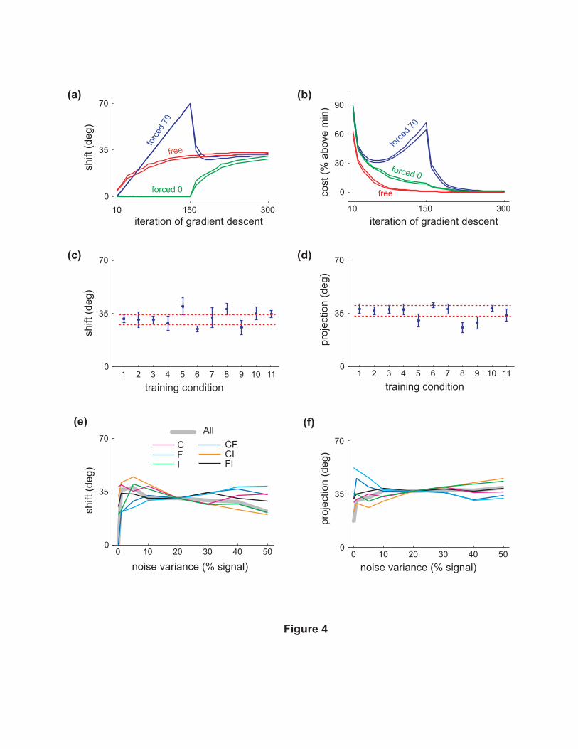
(a)

(c)

(b)

(d)

proj

ectio

n (d

eg)

training condition1 2 3 4 5 6 7 8 9 10

0

35

70

shift

(deg

)

iteration of gradient descent

forc

ed 7

0

forced 0

free

10 150 3000

35

70

cost

(% a

bove

min

)

10 150 300

0

30

60

90

force

d 70

forced 0

free

iteration of gradient descent

shift

(deg

)

1 2 3 4 5 6 7 8 9 100

35

70

training condition

Figure 4

11 11

(e) (f)

proj

ectio

n (d

eg)

noise variance (% signal)0 10 20 30 40 50

0

35

70All

CFI

CFCIFI

shift

(deg

)

0 10 20 30 40 500

35

70

noise variance (% signal)

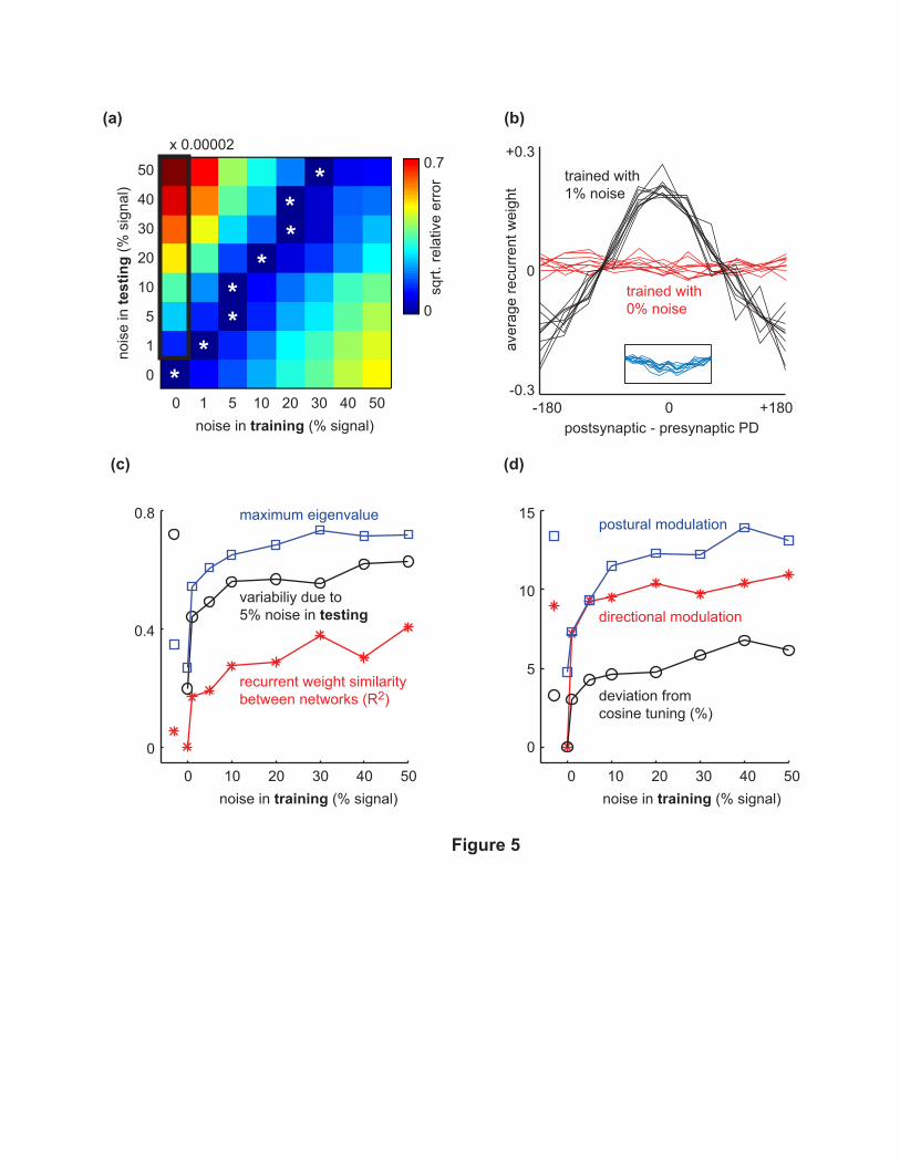
0-180 +180-0.3

+0.3

0

0

0.8

0 20 50noise in training (% signal)

postsynaptic - presynaptic PD

trained with0% noise

trained with1% noise

recurrent weight similaritybetween networks (R2)

variabiliy due to5% noise in testing

10 30 40

ave

rage

recu

rren

t wei

ght

(a) (b)

(c)

Figure 5

0

15

(d)

0 50noise in training (% signal)

2010 30 40

sqrt.

rela

tive

erro

r

maximum eigenvalue postural modulation

deviation fromcosine tuning (%)

directional modulation

1 5

0

50

20

10

30

40

1

5

nois

e in

test

ing

(% s

igna

l)

0.7

0

x 0.00002

**

**

***

*

0 20 50noise in training (% signal)10 30 40

0.4

10

5

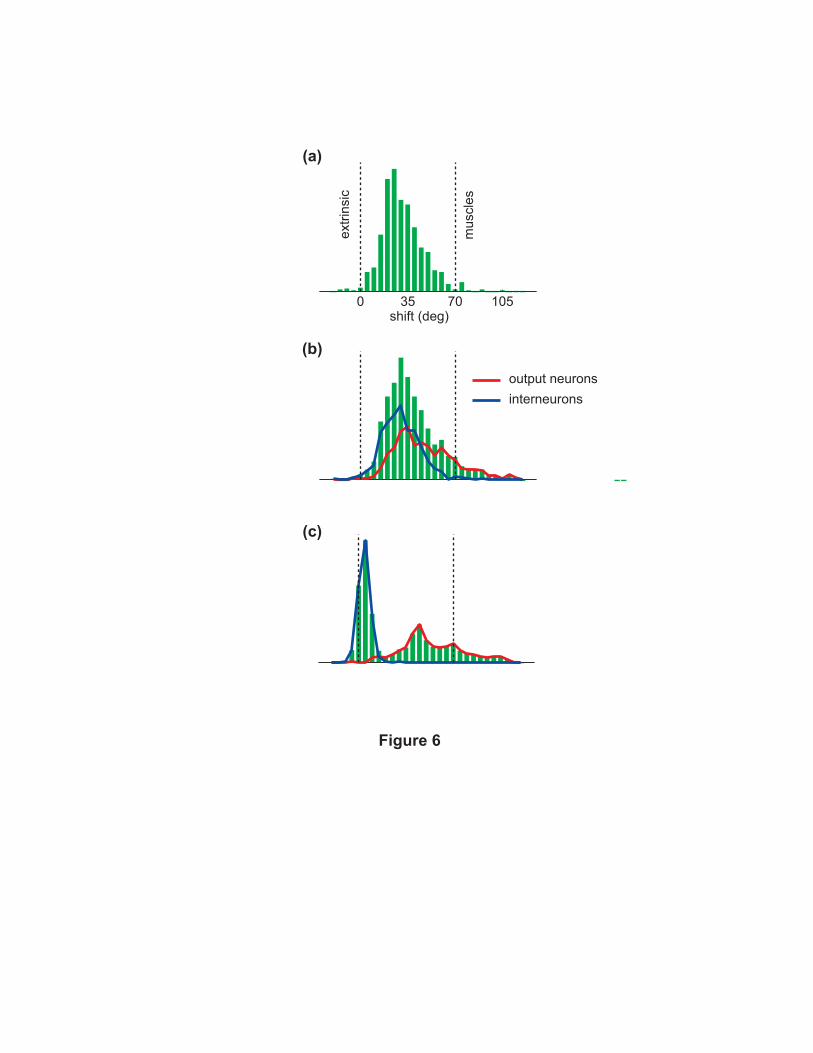
(a)

(c)

(b)

shift (deg)

extri

nsic

mus

cles

0 35 70 105

output neuronsinterneurons

Figure 6