Recruitment, training and career concerns�

Heski Bar-Isaac and Juan-José Ganuzay

NYU and UPF

April 2008

Abstract

We examine training and recruitment policies in a two-period model that nests

two forms of production, "routine" work where ability and e¤ort are substitutes and

"creative" work where they are complements. Alternative ways of improving average

ability have opposite implications for agents�career concerns. While teaching to the

top (training complementary to ability) or identifying star performers increases agents�

career concerns, teaching to the bottom has the opposite e¤ect. The paper also makes

more general comments relating to models of reputation.

Keywords: recruitment, training, career concerns, reputation

JEL Codes: M51, M53, D83, L14

�This paper has circulated under too many titles: "Teaching to the Top and Searching for Superstars","Static E¢ ciency and Dynamic Incentives" and "Reputation for Excellence and Ineptitude". We thankthe Co-editor and two anonymous referees for useful comments that substantially improved the paper andMariagiovanna Baccara, Jordi Blanes, Patrick Bolton, Luis Cabral, Guillermo Caruana, Pablo Casas, An-toine Faure-Grimaud, Leonardo Felli, Esther Hauk, Hugo Hopenhayn, Ian Jewitt, Clare Leaver, AlessandroPavan, Larry Samuelson, Lucy White and audiences at ESSET 2004, IIOC 2004, Università Boconni, ESWC2005, Universitat Autonoma de Barcelona, UCLA and USC for comments and helpful conversations relatingto this work. The �rst author thanks Rutgers University and CEMFI for their hospitality.

yDepartment of Economics, Stern School of Business, NYU, 44 West 4th Street, New York, NY 10012,USA. Tel: 212 998 0533; Fax: 212 995 4218; email heski@nyu.edu and Department of Economics andBusiness, Universitat Pompeu Fabra, Jaume I, 2E82 , Ramon Trias Fargas, 25-27, 08005-Barcelona (Spain)Tel (+34) 93 542 2719; fax (+34) 93 542 1746; email juanjo.ganuza@upf.edu.

1

In the next decade and beyond, the ability to attract, develop, retain and

deploy sta¤ will be the single biggest determinant of a professional service

�rm�s success.

Maister [1997] p.189

1 Introduction

Popular press and academic literature have come to stress the importance of recruitment

and development of sta¤ in industries where human capital plays a critical role.1 This

popular literature tends to recommend recruiting the �best� and training them. There

are, of course, costs as well as bene�ts to recruitment and training. In this paper, we

highlight that there may be indirect costs and bene�ts through the e¤ect on employees�

incentives. Thus, the central contribution of this paper is to highlight that in addition to

a¤ecting the quality of sta¤, training and recruitment policies also play a role in a¤ecting

the behaviour of employees through their career concern incentives.

In human capital intensive industries including professional services such as the law,

audit, consulting, and architecture, career concern incentives are of paramount importance.

As discussed in Fama [1980] and Holmström [1982/99], agents may exert e¤ort in trying

to persuade future employers that they are of high ability, that is, they may be motivated

by career concerns.2 It is clear that their motivation will depend on the beliefs of potential

future employers; and a principal contribution of this paper is to note that recruitment

1This literature includes Michaels et al. [2001], Maister [1997], Smart [1999], Hacker [2001] and no doubtmany others.

2A wide literature has extended and considered applications of the career concerns framework. Mostrelevant to this paper, Dewatripont, Jewitt and Tirole [1999] provide a thorough analysis characterizingthe impact of di¤erent information structures (mappings from ability and e¤ort into observable outcomes).Others have focused on speci�c applications, whose primary e¤ect is to alter such information structures, inparticular through teamwork (Meyer [1994] and Jeon [1996]) and delegation of power (Ortega [2003], Blanes-i-Vidal [2007]). More recently Harstad [2007], Casas-Arce [2005] and Martinez [2005] consider di¤erentmicro-foundations for career concerns models with non-linear returns functions and their implications.

2

and training policies will change these.

In particular, we highlight that while many di¤erent training and recruitment policies

might have the same e¤ect on the average level of ability of employees, they can have very

di¤erent (and indeed exactly opposite) implications for incentives.

Our model allows us to present and discuss two di¤erent kinds of training or produc-

tivity enhancement. One that a¤ects an employee�s �core knowledge�that is valuable for

tasks which do not require e¤ort, and another that raises productivity for work that does

require e¤ort. We show that whichever policy is most e¤ective in raising the overall pro-

ductivity of those workers who are already most productive will lead to higher incentives

for employees. Similarly, recruitment policies that are more focused on �nding the very

best workers lead to higher incentives for employees and recruitment policies that ensure

that the least able are seldom recruited reduce employees�incentives.

There are two channels through which training can have an e¤ect. First, training

that is geared towards the most able increases the dispersion of the possible types of an

employee so that observations are more informative. Second, training the top implies there

is a greater pecuniary payo¤ to revealing yourself to be there. Recruitment policies that

focus on identifying superstars rather than identifying inept performers have similar e¤ects

through both channels.

We can distinguish between di¤erent training policies and highlight that the key is the

e¤ect on the most productive since our model nests two models of production. One in

which ability substitutes for e¤ort (one might think in this case of ability as signifying

knowledge of a routine task) and another in which ability and e¤ort are complements (one

might think of more able agents in this case as more likely to have the inspiration which

allows hard work to reap rewards).

The career concerns literature and most of the reputation literature has viewed e¤ort

3

and ability as substitutes. However, more recent literature on reputational concerns in

e¤ect takes the opposite view and suggests that this view of reputation might lead to

somewhat di¤erent e¤ects.3 In particular Mailath and Samuelson [2001] show that when

reputation is a concern to avoid appearing inept then in a �nite-horizon model reputation

e¤ects cannot arise. Further, Moav and Neeman [2005] suggest that more precise infor-

mation can reduce incentives. We discuss at some length how our di¤erent views of the

production process relate to this recent literature on reputation. Further, we make the

methodological point that when e¤ort and ability are not perfect complements, reputation

e¤ects do arise and are similar to the substitutes case.

2 Model

We introduce a two period model with a continuum of types of agents parameterized by

t 2 [0; 1]. Speci�cally in Period 1 a type t agent will have no strategic decision to make

with probability t and in this case will succeed (for example by producing a high quality

product) with probability � and fail with probability 1 � �. Otherwise (with probability

1� t) the agent must make an e¤ort decision. Note that she only gets to make a strategic

decision when her e¤ort has an e¤ect; or, equivalently, she knows which kind of task she is

performing before she takes her e¤ort decision.4 In this latter case, when she chooses e¤ort

e, she succeeds with probability � + e. Thus overall a t-type agent exerting e¤ort e when

given the opportunity to exert e¤ort would succeed with probability t�+(1� t)(�+e) and

fail otherwise. E¤ort is costly and, speci�cally, exerting e¤ort e costs the agent e2

2 , where

< 1� �.3See, in particular, Tadelis [2002], Mailath and Samuelson [2001] and Bar-Isaac [2007].4Similar results can be obtained when the agent does not know her own type and does not know which

kind of task she faces. If she knows her own type but does not know the kind of task that she faces thendi¤erent types would make di¤erent e¤ort decisions.

4

Let g(t) denote the distribution function for the types of agent and let T denote the

average type (according to the ex-ante beliefs) T =R 10 tg(t)dt and let V =

R 10 (t�T )

2g(t)dt

denote the variance of this prior distribution. This distribution function of types is common

knowledge among the agent and employers.

Employers are risk neutral, value a success at 1 and a failure at 0 and they Bertrand

compete for the agent�s service in each period.5 Moreover, outcomes are observable but

e¤ort is not observable and contracts are incomplete, so that in e¤ect an agent is paid

in advance at a wage which is simply the employers� common belief that the agent will

produce a success.

There are two periods of trade, and outcomes are observed (and beliefs revised) in

between the two periods.6 Speci�cally, timing is as follows:

1. Period 1

(a) employers Bertrand compete for the agent�s service

(b) the agent decides the level of e¤ort if appropriate (that is if it is a task where

e¤ort will make a di¤erence)

(c) success/failure commonly observed

(d) employers update beliefs according to Bayes rule

2. Period 2: employers Bertrand compete for the agent�s service

Notice that in period 2, we could allow the agents the opportunity to exert e¤ort but

no agent would do so. Note that whether the agent knows her type or not would have

5 It is su¢ cient to consider two employers bidding for the services of a single employee. More generally,the assumption that employers Bertrand compete for the product is not crucial, similar results would hold solong as the price paid was increasing in the customers�expected likelihood that the agent will be successful.

6One need not take the two periods of the model literally, rather the second period can be thought ofas a reduced form payo¤ for a given reputation level, albeit one that is linear in the reputation.

5

no e¤ect on this model since she has no ability to signal her type (we rule out long-term

and outcome contingent contracts) and at the point where an agent has to make an e¤ort

decision then the problem is identical for all types.

We suppose that the agent weighs the two periods equally and maximizes the sum

of pro�ts for the two periods. We solve for the e¤ort exerted in the Perfect Bayesian

equilibrium.

2.1 Interpreting the model

It is worth highlighting that type t captures the agent�s likelihood of getting an opportunity

to engage in strategic behaviour. One cannot interpret a high t as low or high ability until

all the parameters of the model are speci�ed

The model is intended to re�ect that agents might be confronted with a variety of

di¤erent tasks, and the nature of the particular task undertaken is unobserved by employers.

For example, employers hiring consultants �nd it di¢ cult to determine the extent to which

the project that they are assigning is a complex one or a simple one. Similarly, the di¢ culty

of the project depends on the consultant�s ability and experience. Depending on the value

of �, the model allows for somewhat di¤erent interpretations of the productive process and

of the interpretation of high values of t as re�ecting high or low ability.

Speci�cally, when � is su¢ ciently high, high t re�ects high ability; an agent with a high

value of t �nds it costless to succeed in a wide range of tasks, in this case ability and e¤ort

are substitutes and an agent would like employers to believe that she has a high value of t.

One could think of this case as representing �routine�work, where more able workers know

how to do more things and if they know how to perform the task that they are assigned

they will succeed with high probability.7 If they do not have the requisite knowledge they

7Another interpretation for the high � case is that agents with a high t get it �right �rst time�, but forall agents when they do not, there is the opportunity of exerting e¤ort to try to ��x mistakes�.

6

could exert e¤ort to acquire it, by reading the appropriate manuals for example. Examples

include translation work, mechanics, and routine work in low levels of management in an

organizational hierarchy.

In contrast, when � is su¢ ciently low, then one can think of agents for whom (1� t) is

higher as being more able, and e¤ort and ability as complements. In this case even if the

agent has some understanding of the task, exerting e¤ort will still improve the outcome,

however if she has no understanding of the task then she will surely fail. Here, one needs

some ability in order to have any chance of success (one needs ability to have the �ash of

inspiration) but this in itself will not guarantee success, hard work is also required. This

may be more appropriate for creative work, such as writing a Ph.D., writing advertisements

or high level management which is not routine.

Note, that in the case that � = 0, the agent would prefer employers to believe that she

is a type with a low value of t and so when � = 0, one should think of agents with low

values of t as more able.

In application, of course many jobs will include elements of both creative and routine

work, however for di¤erent jobs or at di¤erent times in an individual�s career (or within an

organizational hierarchy) it will be more appropriate to think of work as primarily of one

or other of these two production types.

In both these cases we can think of more able agents as having facility in some tasks

but not in others. The di¤erence in productivity for a task in which one has facility and in

which one does not when exerting no e¤ort (which is the case in period 2) is simply given

by j�� �j.

7

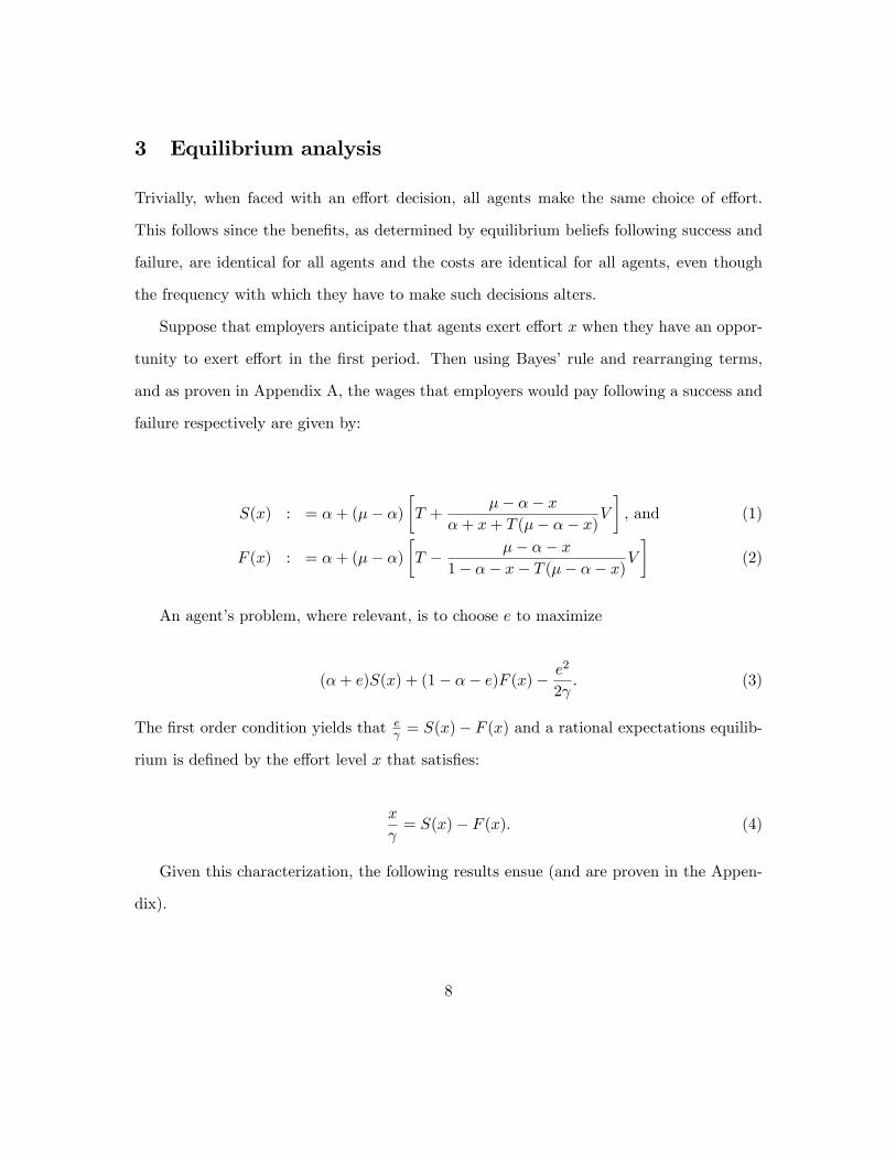
3 Equilibrium analysis

Trivially, when faced with an e¤ort decision, all agents make the same choice of e¤ort.

This follows since the bene�ts, as determined by equilibrium beliefs following success and

failure, are identical for all agents and the costs are identical for all agents, even though

the frequency with which they have to make such decisions alters.

Suppose that employers anticipate that agents exert e¤ort x when they have an oppor-

tunity to exert e¤ort in the �rst period. Then using Bayes�rule and rearranging terms,

and as proven in Appendix A, the wages that employers would pay following a success and

failure respectively are given by:

S(x) : = �+ (�� �)�T +

�� �� x�+ x+ T (�� �� x)V

�, and (1)

F (x) : = �+ (�� �)�T � �� �� x

1� �� x� T (�� �� x)V�

(2)

An agent�s problem, where relevant, is to choose e to maximize

(�+ e)S(x) + (1� �� e)F (x)� e2

2 . (3)

The �rst order condition yields that e = S(x)� F (x) and a rational expectations equilib-

rium is de�ned by the e¤ort level x that satis�es:

x

= S(x)� F (x). (4)

Given this characterization, the following results ensue (and are proven in the Appen-

dix).

8

Proposition 1 Equilibrium e¤ort is well-de�ned and unique. Further (i) The equilibrium

e¤ort e� is lower than the e¢ cient solution efb = . (ii) If � > � then � > �+ e�.

Note in particular that since equilibrium e¤ort is unique, comparative statics exercises

are well de�ned and can be explored. Note, further, as discussed at some length in Section

2.1, that in the case where � is high (� > �) or � is low (� < �) the model has natural

interpretations as capturing �routine�and �creative�production respectively. Finally, note

that when conducting these comparative statics results, we assume that parameters remain

common knowledge among all agents, employers and potential employers; in particular, in

the context of Sections 5.1 and 5.2, when we consider a �rm choosing a recruitment or

training strategy, it is assumed that these choices are known and understood by all market

participants.

4 Comparative Static Results

The �rst result is a very intuitive one, if e¤ort is less costly then the agent will exert more

e¤ort (when relevant) in equilibrium.

Proposition 2 The equilibrium e¤ort e� is increasing in

Proof. It is convenient to de�ne h(x) := S(x)� F (x)� x .

Note that by the arguments of the proof of Proposition 1, h(x) is decreasing in the

range (0; ). Using the Implicit Function Theorem de�

da = �@h(a)@a

@h(e)@e

and since @h(e)@e < 0, the

sign of de�

da is simply the sign of@h(x;a)@a and so it is su¢ cient to consider that expression for

a = , that is to consider @h(x; )@ . Recall

h(x) = �x + S(x)� F (x). (5)

9

and so taking the derivative with respect to , we obtain

@h(x; )

@ =x

2> 0 (6)

Therefore, we conclude that the optimal e¤ort e� is increasing in :

Next we turn to comparative statics with respect to V . The intuition here is clear, the

greater the variance in the distribution of types, the more scope that the observation of a

success or failure has to shift beliefs and the associated rewards. This is a familiar intuition

(from Holmström [1982/99] for example). Here we highlight that the result depends on V

and no other characteristics of the distribution (in particular, we do not restrict that g(:)

be Normal).

Proposition 3 The optimal e¤ort e� is increasing in V .

Proof. As in the proof of Proposition 2, the sign of de�

dV is simply the sign of @h(x;V )@V .

Taking the derivative with respect to V yields:

@h

@V=@(S � F )@V

=(�� �)(�� �� x)

[(�� �� x)T + (�+ x)] [(1� �� x)� (�� �� x)T ] > 0. (7)

Notice that while increasing V or has a clear monotonic e¤ect on e¤ort, the compar-

ative statics with respect to other parameters depend on which of the two interpretations

alluded to in the description of the model in Section 2 applies, that is, whether an agent�s

reputational concern is to try to convince employers that she is a �high t�type or a �low

t�type.

First, we consider comparative statics with respect to �. Underlying the following result

are two e¤ects, �rst that it is more important to show oneself to be at the top of the ability

10

distribution (or having facility in a greater range of tasks that is high t in the case when �

is high, low t in the case when � is low) the greater the di¤erence between the productivity

of an agent in a task in which she has facility and her productivity in one which she does

not, regardless of her level of e¤ort (that is the greater is j�� �� xj for all e¤ort levels x).

Secondly as j�� �� xj increases then an observation of success or failure becomes more

informative. We distinguish explicitly between these two e¤ects in the discussion in Section

5.3. In particular therefore when � is high, one would expect that an increase in � should

reduce e¤ort, but when � is low, it would increase equilibrium e¤ort. Note however that in

all cases, increasing � raises the average productivity of the agent. Similar considerations

apply with regard to comparative statics in �. The proposition below demonstrates that

these intuitions are borne out.

Proposition 4 Equilibrium e¤ort is increasing in � but decreasing in � when � < � but

decreasing in � and increasing in � when � > �.

Proof. As in the proof of Proposition 2, it is su¢ cient to consider @h@� , and@h@� .

@h(x;�)@� = @(S�F )

@� =h

(����x)V(����x)T+�+x +

(����x)V1���x�(����x)T

i+(�� �)

h(�+x)V

((����x)T+�+x)2 +(1���x)V

(1���x�(����x)T )2i (8)

Notice that the denominators are always positive. Since, by Proposition 1(ii) when � > �

then also � > � + x, it follows that in this case @(S�F )@� > 0. If instead, � < �, since by

Proposition 1 x > 0 then @(S�F )@� < 0.

Similarly

@h(x;�)@� = @(S�F )

@� = �h

(����x)V(����x)T+�+x +

(����x)V1���x�(����x)T

i+(�� �)

h�V �

((����x)T+�+x)2 +�V (1��)

(1���x�(����x)T )2i (9)

11

Again the denominators are always positive and if � > �, then @(S�F )@� < 0 since (����x)

and (�� �) are positive, similarly if � < �, then @(S�F )@� > 0.

5 Discussion

5.1 Targeted training or productivity enhancement

Our model allows for di¤erent kinds of training, or productivity enhancing technology. In

the model, increasing � and increasing � can both increase the ability of agents, and can

readily be interpreted as the result of training directed towards di¤erent types of agents or

di¤erent kinds of productivity-enhancing technologies. A �rm may wonder whether there

is much di¤erence, for example, in giving employees access to a database that expands

their core knowledge (increasing �) or giving them access to software that allows for more

e¤ective work (increasing �).

As demonstrated in Proposition 4, these two means of increasing average ability have

exactly opposite e¤ects for equilibrium e¤ort. In particular for low values of � when an

agent would like employers to believe that she is a �low t�type then raising the ability of a

�low t�type relatively more than raising the ability of a �high t�type (either by decreasing

� or by increasing �) heightens this reputational concern. As discussed below, it does so

through two channels, by raising the pecuniary value of showing oneself to be a higher type

and by making the outcome more informative about the agent�s type.

Similarly in the case where � is high, then agents with high t are the most productive

and a greater distinction between the most able and the least able (here by increasing

� or decreasing �) will heighten the reputational concern for agents seeking to convince

consumers that they are the most able.

Thus in all cases raising the productivity of the most able agents (or reducing the

12

productivity of the least able) increases the equilibrium e¤ort.

5.2 Recruitment policies and searching for superstars

While training as described above a¤ects the productivity of a given type and thereby

a¤ects the prior beliefs about an agent�s productivity, interviewing and recruitment policies

directly a¤ect the initial belief about the distribution of types g(t). When employers seek

recruitment policies which select better agents, there are various ways in which this can

be achieved. Consider the case when � is high (so that types with high values of t are the

better agents); a recruitment policy that selects better agents will lead to a shift in the

prior distribution from g(t) with associated T and V , to a di¤erent prior distribution g0(t)

with associated T 0 > T and V 0. Following Proposition 2, among all policies with the same

e¤ect on average ability (that generate the same T 0), an employer would prefer to choose

a policy that raised rather than reduced the variance of the distribution. When superstars

and disastrous potential recruits are rare, then it follows that employers concerned with

employees�e¤orts would be better using recruitment policies that concentrated more on

ensuring that any potential superstars were recruited than ruling out the worst of the

applicants.8

8For example, suppose that with no recruitment policy, types are distributed according to the degeneratedistribution g(0) = 1

10; g( 1

2) = 4

5and g(1) = 1

10so that T = 1

2and V = 1

20. Now consider, two recruitment

policies which raise the average ability, one does so by reducing the probability of recruiting disasters.Speci�cally Policy A leads to the distribution gA(0) = 1

20, gA( 12 ) =

1720, and gA(1) = 1

10so that TA =

2140and VA = 1

20( 2140)2 + 17

20( 140)2 + 1

10( 1940)2 = 59

1600. Policy B increases the probability of identifying

superstars and leads to the distribution gB(0) = 110, gB( 12 ) =

34, and gB(1) = 3

20, then TB = 21

40and

VB = 110( 2140)2 + 3

4( 140)2 + 3

20( 1940)2 = 99

1600. Since VB > VA it follows by Proposition 2 that, while both

policies raise average ability equally, the latter policy would lead to greater equilibrium e¤ort compared tothe �rst and so would be preferred.

13

5.3 The information and value e¤ects

By adapting the model slightly to suppose that in period 2 a type t agent succeeds with

probability t�0+(1� t)�0, we can distinguish between two channels through which changes

in ability as discussed in Proposition 4 and Section 5.1 a¤ect incentives. Speci�cally, in

this modi�ed model S � F = (�0 � �0)h

(����x)V(����x)T+�+x +

(����x)V1���x�(����x)T

iand similar

qualitative results apply.

Proposition 5 Equilibrium e¤ort is increasing in � and �0 but decreasing in � and �0

when �; �0 < � but decreasing in � and �0 and increasing in � and �0 when �; �0 > �.

Proof. Similar to the proof of Proposition 4, it is su¢ cient to consider @(S�F )@� , @(S�F )@�0 ,

@(S�F )@� ,and @(S�F )

@�0 .

First@(S � F )@�0

=(�� �� x)V

(�� �� x)T + �+ x +(�� �� x)V

1� �� x� (�� �� x)T (10)

which is negative when � < � but positive when � > �. Similarly,

@(S � F )@�0

= � (�� �� x)V(�� �� x)T + �+ x �

(�� �� x)V1� �� x� (�� �� x)T (11)

which is positive when � < � but negative when � > �.

Next

@(S � F )@�

= (�0 � �0)�

(�+ x)V

((�� �� x)T + �+ x)2+

(1� �� x)V(1� �� x� (�� �� x)T )2

�, and

(12)@(S � F )@�

= (�0 � �0)�

�V T((�� �� x)T + �+ x)2

+�V (1� �)

(1� �� x� (�� �� x)T )2

�. (13)

Similarly to the proof of Proposition 4, the derivatives have the signs claimed in the

relevant parameter ranges.

14

Thus Proposition 5 demonstrates that the overall e¤ect of changing the abilities of

types through changes to � and � described in Proposition 4 can be decomposed into two

distinct mechanisms.

First consider the comparative statics with respect to the second period productivities

�0, and �0. Fixing some e¤ort level, then the beliefs about the type of an agent following

either a success or a failure do not change as �0 or �0 changes. However, since the belief

that the agent is excellent following a success is higher than it is following a failure, raising

(lowering) �0 in the case where �0 > � (where �0 < �) increases S� the agent�s wage fol-

lowing a success� by more than it increases F , the wage following failure. Since incentives

are stronger the greater the di¤erence between S and F , an increase in �0 therefore raises

incentives. A similar argument applies for �0. Notice that changing �0, and �0 does not

a¤ect the inferences that employers draw from the outcomes (in equilibrium when they

correctly anticipate x) but they a¤ect the value to the agent of being thought of as a par-

ticular type. We therefore term this channel for in�uencing an agent�s incentives a �value

e¤ect�.

We now turn to the comparative statics with respect to the �rst period productivities

through changes in �, and �. If the beliefs about the type of the agent are �xed, then

increasing �, and � has no e¤ect whatsoever on the value of the agent in Period 2. Changing

� and �, however, can a¤ect the inferences that employers draw from an observation of

success or failure, we therefore term such changes as having an �information e¤ect�. In

particular, intuition can be drawn from the observation that for a �xed level of e¤ort,

increasing (reducing) � in the case where � > � (where � < �) increases the probability that

�better types� generate success and decreases the probability that they generate failure.

Therefore, conditional on observing on a success, employers believe that the agent is more

likely to be at the top of the ability distribution and so S is higher, while conditional

15

on observing a failure, employers believe that the agent is less likely to be at the top of

the distribution and so F is lower. In particular, therefore, (S � F ) increases. Similar

arguments apply with regard to changes in �.

5.4 Reputation for excellence or ineptitude

This paper relates to a wider literature on reputation. Much of the economic literature

on reputation has focused on a reputation for excellence (trying to show that you are a

type who always does well, or where reputation is about �who you�d like to be�).9 In

these models, the �most able� are non strategic and implicitly, they are assumed to be

somewhat unusual or scarce, so for example with that view of the world, one might expect

general �untargeted� training to have little e¤ect on them. Such training would reduce

career concern incentives.

More recent literature (Mailath and Samuelson [2001], Tadelis [2002], Bar-Isaac [2007])

and common intuition suggests that often reputational concerns might also relate to avoid-

ing a reputation for ineptitude (trying to show that you are not an inept type who always

does badly or where reputation is about �who you�re not�) where the top of the distribu-

tion is the strategic type, and the bottom of the distribution is an inept types whom one

might expect to be little a¤ected by training.

The distinction between these two approaches to reputation has been forcibly made

by Mailath and Samuelson [1998] who highlight, in particular, that the latter view of

9Following Kreps and Wilson [1982] and Milgrom and Roberts [1982] and later Fudenberg and Levine[1989], the formal economic literature on reputation has been used primarily to discuss beliefs about thetype of the agent. Previous literature (Klein and Le­ er [1981] for example) and a great deal of intuition hasalso used the term in a somewhat looser fashion to consider sustaining certain actions in in�nitely repeatedgames. As highlighted in Fudenberg and Levine [1989] this corresponds closely to the notion of reputationwhere reputation is a concern to show that you�re a �Stackelberg� type� that is a type whose behavior astrategic agent would like to promise to commit to� similar to what we term later in this note a reputationfor excellence. See Bar-Isaac and Tadelis [2007] for a review of this literature and alternative approachesto reputation.

16

reputation leads to increasing certainty about the agent�s type over time and so reputational

incentives disappear over time unless type uncertainty is continually introduced.10

In practice, it is far from obvious whether it is more appropriate to think of agents as

particularly concerned that others should think them to be excellent or that they should

not think them to be inept. However, as we illustrate, modelling reputational concerns in

these two ways can lead to opposite conclusions.

This paper highlights an important distinction between the two approaches in a simple

two-period model. Speci�cally, following the intuition of the paragraphs above, making

the strategic agent more e¢ cient diminishes reputational concerns (reducing e¤ort) when

reputation is about excellence but increases reputational concerns when reputation is about

ineptitude.

To see this more clearly consider setting � = 1 and the degenerate distribution g(0) =

1�p and g(1) = p. This corresponds to a fairly typical model where type t = 0 corresponds

to the strategic type whose reputational concern is to try to convince customers that she

is the �excellent�or Stackelberg type. Following Proposition 2, in this case improving the

strategic agent by raising � would reduce e¤ort.

In contrast suppose that a strategic agent�s reputational concern is to avoid a reputation

for ineptitude. This corresponds to the model where � = 0 with g(0) = 1� p and g(1) = p

and in this case improving the strategic agent by raising � would increase equilibrium

e¤ort.10Further in Mailath and Samuelson [1998], the model is constructed in such a way that there is unravelling

so that if there are no reputational incentives at some point, there are no such incentives throughout.The more general point on reputational incentives disappearing over time without some kind of replen-

ishment of type uncertainty applies more widely. Indeed, Cripps, Mailath and Samuelson [2004] show thisto be the case unless actions are perfectly observable, even in the case when reputation is about excellenceand a competent agent can perfectly mimic an excellent agent (though incentives may disappear only inthe very long run).Bar-Isaac [2007] suggests an endogenous mechanism to maintain type uncertainty by allowing agents to

choose to work in teams. Liu [2007] supposes that receivers must pay to observe history. This also providesan endogenous mechanism which limits an audience�s certainty about type.

17

It is worth noting that in those papers that have considered something akin to the inept

type we consider in this paper (in particular Diamond [1989], Mailath and Samuelson [1998],

Tadelis [2002] and Bar-Isaac [2007]), there are no reputational incentives from trying to

avoid a reputation for ineptitude or gain a reputation for competence per se.11 Essentially

this is because in the notation of this paper they have taken � = 0.

5.5 Many periods

Extending the model beyond two periods is not straightforward. First, in a multi-period

model, the agent�s belief about herself (and in particular whether she knows her type)

will make a di¤erence. This belief will a¤ect her expectations of continuation values in

all periods up until the last one, and so a modeler must take a stance on this belief.12

Second, with many time periods and di¤erent types, there are many equilibrium conditions

that need to be simultaneously satis�ed. For example, a decision on how much e¤ort

to exert with two periods remaining must take into account not only the agent�s type

but also expectations of what e¤orts she will take (and what e¤orts the public would

anticipate and so compensate) in subsequent periods. Similarly, e¤orts in later periods

depend on reputations that arise as a result of e¤orts in earlier periods. In contrast to the

single equilibrium condition (4) that appears in this model, in a multi-period extension one

needs to solve a system of non-linear equations. This makes an analytical characterization

challenging, though for a �nite-period (if not an in�nite horizon) model one can proceed

by backwards induction, where the analysis of the penultimate period would be identical

11 In those papers, it is only useful to be thought of as a competent type if you can somehow also committo exerting e¤ort. Diamond also allows for an inept type that always fails, but has a strategic type forwhom � = 0, Cabral and Hortacsu [2004] is an exception in supposing that � 6= 0.12Note also that if the agent does not know her type initially, she will learn it at a di¤erent rate to

customers, as she observes whether or not she has made a strategic decision and the level of e¤ort (whichwould be relevant for considering o¤-equilibrium deviations) and not just the outcome, which is all that thepublic observes.

18

to our two-period model.

We numerically analyze a three period version of our model in a Appendix B, in which

all the qualitative results of the two period model appear to be robust.13 Nevertheless,

although a number of forces operate in the same way and dominate in the many numerical

parametrizations we have explored, there are some subtle and potentially counter-acting

mechanisms. These can be understood by distinguishing between information and value

e¤ects,as we did in Section 5.3.

The information e¤ect works as described above: increasing � in the case that e¤ort and

ability are complements or � when they are substitutes suggests that, all else equal, out-

comes are more informative signals on ability. As long as the value of entering the second

period with a given reputation is non-decreasing, then since outcomes are more informa-

tive, the agent will be induced to exert more e¤ort. In the case where e¤ort and ability

are substitutes, then following Proposition 1(ii) the agent always prefers that potential

employers think she is better (and so more likely to be succeeding with probability �) than

exerting e¤ort (in particular the very best agent t = 1 has no opportunity to exert e¤ort).

In this case therefore, the value with two remaining periods is indeed non-decreasing in

reputation. It is theoretically possible however, that it can be non-monotonic when e¤ort

and ability are complements. In this case, even the best possible agent (that is one of type

t = 0) would prefer to commit to exerting e¤ort. With no means to do so, the agent may

13Note that there is an additional complication: it is not clear what would constitute an analogous resultin the case of a mutli-period extension. There are a number of di¤erent e¤orts that characterize equilibrium(speci�cally equilibrium e¤ort would be a function of the agent�s belief about her type, the public�s beliefabout the agent�s type and the number of periods remaining). In considering comparative statics, it isnot clear what the appropriate multi-period analogue of our results should be: e¤ort in the �rst periodgiven an initial reputation (prior distrinution), e¤orts in any period, given an initial reputation, or perhapsof greater interest might be the overall lifetime expected e¤ort. Although we have not included it in themodel, this would be particularly relevant in an environment where the initial employers competed bothwith respect to wages and recruitment/training policies. Employees would compete by o¤ering workersrecruitment/training policies that led to more e¢ cient decisions for lifetime earnings.Our results appear to be robust with respect to all of these measures.

19

bene�t more from uncertainty about her ability which induces her to exert e¢ cient e¤ort

than from having potential employers certain that she is excellent (and thereby dampening

her incentives for e¤ort). Although, this is a theoretical possibility, we have been unable

to �nd numerical examples.14

In both cases, where e¤ort and ability are substitutes or complements, the value e¤ect

can be decomposed into two e¤ects. Consider, increasing � in the complements case for

the second and third periods but not for the �rst period. First, one can think of a �direct�

value e¤ect, �better�agents are more productive as in the main model and so agents should

seek to prove themselves to better, leading to similar comparative statics. However, there

is an additional �indirect� value e¤ect, which is that second period e¤orts are altered,

as described in the main model. Speci�cally, these increase at all reputation levels. It

is theoretically conceivable that second period e¤orts might increase so much more for

a second period reputation that arises following a �rst period failure than a �rst period

success that it dampens �rst period incentives.

Overall, therefore the �direct�value e¤ect boost e¤orts, as will the information e¤ect

in the case where e¤ort and ability are substitutes. Although, the �indirect�value e¤ects

(in both cases) and the information e¤ect when e¤ort and ability are complements might

possibly work in the opposite direction, we have been unable to �nd examples in which our

qualitative results on comparative statics are overturned in a three period extension of the

model.15

14Further, there is intuition to suggest that this cannot arise. Such a result requires that the e¤ortgenerated in equilibrium is valuable as compared to �raw ablity� (�). However, raw ability must besigni�cant enough to generate equilibrium e¤ort in the �rst place.15Given the intuitions in this section, we have searched in particular in the e¤ort and abilities as com-

plements case (where the information e¤ect is ambiguous) and in the case where the initial reputation ishigh (that is where the agent is very likely to be strategic) since here following �rst period success there islikely to be much less uncertainty (and so relatively low e¤ort) as compared to failure.

20

6 Summary

At heart this paper highlights the simple observation that the distribution of prior beliefs

is a crucial determinant of reputational incentives. There are numerous considerations

which a¤ect such prior beliefs, including for example contemporaries and social peers.

Further, there are many policies that �rms undertake (in particular, we have focused on

training and recruitment policies) which a¤ect the shape of the distribution of these priors.

Di¤erent policies which a¤ect the mean ability in the same way can have exactly opposite

implications for reputational concerns.

References

[1] Bar-Isaac, Heski (2007) �Something to prove: Reputation in teams,�RAND Journal of Eco-

nomics, forthcoming

[2] Bar-Isaac, Heski and Steven Tadelis (2007) �Seller Reputation,�working paper

[3] Blanes-i-Vidal, Jordi (2007) �Delegation of decision rights and the winner�s curse,�Economics

Letters, 94(2), 163-9.

[4] Cabral, Luís and Ali Hortaçsu (2004) �The Dynamics of Seller Reputation: Theory and Evi-

dence from eBay,�working paper, NYU

[5] Casas-Arce, Pablo (2005): �Career Tournaments,�working paper, Oxford University

[6] Cripps, Martin W., George J. Mailath and Larry Samuelson (2004) �Imperfect Monitoring

and Impermanent Reputation,�Econometrica, 72, 407-432

21

[7] Dewatripont, Mathias, Ian Jewitt; Jean Tirole (1999) �The Economics of Career Concerns,

Part I: Comparing Information Structures,�The Review of Economic Studies, Vol. 66, No. 1,

Special Issue: Contracts, 183-198

[8] Diamond, Douglas W. (1989) �Reputation Acquisition in Debt Markets,� The Journal of

Political Economy, 97, 828-862

[9] Fama, Eugene F. (1980) �Agency Problems and the Theory of the Firm,� The Journal of

Political Economy, 88 (2), 288-307

[10] Fudenberg, Drew and David K. Levine (1989) �Reputation and Equilibrium Selection in Games

with a Patient Player,�Econometrica, 57, 759-778

[11] Hacker, Carol A. (2001) How to Compete in the War for Talent : A Guide to Hiring the Best,

DC Press

[12] Harstad, Bard (2007) �Organizational Form and the Market for Talent,� Journal of Labor

Economics, forthcoming

[13] Holmström, Bengt (1999) �Managerial Incentive Problems� A Dynamic Perspective,� The

Review of Economic Studies, 66, 169-182; (originally appeared (1982) in Essays in Honor of

Professor Lars Wahlback).

[14] Jeon, Seonghoon (1996) �Moral Hazard and Reputational Concerns in Teams: Implications

for Organizational Choice,�International Journal of Industrial Organization, 14, 297-315

[15] Klein, Benjamin, and Keith B. Le­ er (1981) �The Role of Market Forces in Assuring Con-

tractual Performance,�Journal of Political Economy, 89, 615-641

[16] Kreps, David and Robert Wilson (1982) �Reputation and Imperfect Information,�Journal of

Economic Theory, 27, 253-279

22

[17] Liu, Qingmin �Information Acquisition and Reputation Dynamics,�working paper

[18] Mailath, George J. and Larry Samuelson (1998) �Your Reputation Is Who You�re Not, Not

Who You�d Like To Be,�CARESS working paper 98-11, University of Pennsylvania

[19] Mailath, George J. and Larry Samuelson (2001) �Who Wants a Good Reputation?� The

Review of Economic Studies, 68, 415-441

[20] Maister, David H. (1997): Managing The Professional Service Firm, Free Press; Reprint

edition

[21] Martinez, Leonardo (2005): �Reputation and Career Concerns,�working paper, Federal Re-

serve Bank of Richmond

[22] Meyer, Margaret A. (1994): �The Dynamics of Learning with Team Production: Implications

for Task Assignment,�The Quarterly Journal of Economics, 109 (4), 1157-1184

[23] Michaels, Ed, Helen Hand�eld-Jones, Beth Axelrod (2001) The War for Talent, Harvard

Business School Press

[24] Milgrom, Paul and John Roberts (1982) �Predation, Reputation and Entry Deterrence,�Jour-

nal of Economic Theory, 27, 280-312

[25] Moav, Omer and Zvika Neeman (2005) �The Quality of Information and Incentives for E¤ort,�

Hebrew University Working Paper No. 2005-01

[26] Ortega, Jaime (2003) �Power in the Firm and Managerial Career Concerns,�Journal of Eco-

nomics and Management Strategy, Vol. 12 (1), 1-29

[27] Smart, Bradford D. (1999): Topgrading: How Leading Companies Win by Hiring, Coaching

and Keeping the Best People, Prentice Hall Art

23

[28] Tadelis, Steven (2002) �The Market for Reputations as an Incentive Mechanism,�The Journal

of Political Economy, 110, 854-82

[29] Tirole, Jean (1996) �A Theory of Collective Reputations (with Applications to the Persistence

of Corruption and to Firm Quality),�The Review of Economic Studies, 63, 1-22

A Derivation of S(x) and F (x)

Suppose that the equilibrium e¤ort level is given by x. Then a type t agent generates success inthe �rst period with probability

�t+ (1� t)(�+ x) = (�� �� x)t+ (�+ x), (14)

and generates a failure with probability

1� �t� (1� t)(�+ x) = 1� �� x� t(�� �� x). (15)

By Bayes rule, the probability density function given a success and given the belief that agentsexert e¤ort x in the �rst period can be written down as

s(t; x) =(�� �� x)t+ �+ xR 1

0[(�� �� x)t+ �+ x] g(t)dt

g(t) =(�� �� x)t+ �+ x(�� �� x)T + (�+ x)g(t), (16)

and the probability density function given a failure in the �rst period is

f(t; x) =1� (�� �� x)t� (�+ x)R 1

0[1� (�� �� x)t� (�+ x)] g(t)dt

g(t) =1� (�� �� x)t� (�+ x)1� (�� �� x)T � (�+ x)g(t). (17)

In the second period, an agent of type t will exert no e¤ort and so succeed with probability�t + (1 � t)� = t(� � �) + �. In particular it follows, that if employers believed that the typeswere distributed according to h(:) going into period 2 then they would be willing to pay the agentR 10(t(�� �) + �)h(t)dt.It follows that the wage that employers would pay following success and failure respectively are

given by:

S(x) =

Z 1

0

(t(�� �) + �)s(t; x)dt = (�� �)E [tjS; x] + �, and (18)

F (x) =

Z 1

0

(t(�� �) + �)f(t; x)dt = (�� �)E [tjF; x] + �, (19)

24

where

E [tjS; x] =

Z 1

0

ts(t; x)dt = T +(�� �� x)V

(�� �� x)T + (�+ x) , and (20)

E [tjF; x] =

Z 1

0

tf(t; x)dt = T � (�� �� x)V(1� �� x)� (�� �� x)T . (21)

Proof. of Proposition 1We begin by proving (i) and (ii) for any equilibirium e¤ort e�.(i) Notice that S(x) < 1 for all x and F (x) > 0 for all x; so in particular S( )�F ( ) < 1, then

the equilibrium e¤ort levele�

= S(e�)� F (e�) < 1 =) e� < (22)

(ii) For contradiction suppose that �� �� e� < 0; then consider

S(e�)� F (e�) = (�� �)(�� �� e�)V[�T + (�+ e�)(1� T )] [1� �� e� � (�� �� e�)T ] (23)

Note that 1 � � � e� > T (� � � � e�) since T < 1 and 1 > � so the denominator is positiveand since � > � and ���� e� < 0 it follows that S(e�)�F (e�) < 0 but then it is impossible thatS(e�)� F (e�) = e�

> 0, which is our desired contradiction.It su¢ ces to show that there exists a unique solution for the equation (4), which is in the range

(0; ).Let h(x) = �x

+S(x)�F (x). The equilibrium e¤ort is then given by the solution of h(e�) = 0for e� 2 (0; ):

Note that h(0) = S(0)�F (0) > 0 and given (i) and (ii), h(0) > 0 and h( ) < 0: Moreover, h(x)is continuous, and thus there exists at least one solution in the range (0; ).

In order to demonstrate uniqueness, �rst take the derivative of (S � F ):

d(S � F )dx

= �(�� �)V [ �

[(�� �� x)T + (�+ x)]2+

(1� �)[(1� �� x)� (�� �� x)T ]2

] (24)

Then if � > �, d(S�F )dx < 0 and so h(x) is monotonically decreasing in the range (0; ) and sothe solution must be unique.

If � < � then d(S�F )dx > 0 and so potentially, h(x) could be increasing in some subset of (0; )

(note that since h(0) > 0 and h( ) < 0 at must be decreasing in some of the range). However, we

know that, when � < �, d3h(x)dx3 > 0 since

d3h(x)

d3x= (�� �)V [ �6(1� T )2

[(�� �� x)T + �+ x]4+

(1� �)6(1� T )2

[1� �� x� (�� �� x)T ]2] > 0 (25)

Suppose for a contradiction that h(e�) = 0 has a number of solutions 0 < e1 < : : : < eN < .Then �rst note that since h(0) > 0 and h( ) < 0 then N must be an odd number. In particulartherefore if there are multiple solutions to h(e�) in the range then there must be at least three.However h(0) > 0 and 0 < e1 < e2 < e3 with h(e1) = h(e2) = h(e3) = 0 requires dh(e1)

dx < 0,

25

dh(e2)dx > 0 and dh(e3)

dx < 0 which contradicts d3h(x)d3x > 0.

B Three period, two type model

There are two types of agents parameterized by 0 � t � T � 1.Production is as in the main model. Speci�cally in each period, a type i agent will have

no strategic decision to make with probability i and in this case will succeed (for example byproducing a high quality product) with probability � and fails with probability 1 � �. Otherwise(with probability 1�i) the agent must make an e¤ort decision. In this latter case, when she choosese¤ort e, she succeeds with probability � + e. Thus overall an i-type agent exerting e¤ort e whengiven the opportunity to exert e¤ort would succeed with probability i� + (1 � i)(� + e) and failotherwise. E¤ort is costly and, speci�cally, exerting e¤ort e costs the agent e2

2 .Let rj denote the public�s belief that the agent is of type t at time j. Note that in contrast to

the two period case, for multiple periods, it will make a di¤erence whether we assume that agentsknow their own types or not. Here we assume that agents do not know their own types initially.Therefore if they observe that they have an e¤ort decision to make they gain some informationabout their type. We can write the private, intermediate belief after observing an opportunity toexert e¤ort as p1 =

r1(1�T )r1(1�T )+(1�r1)(1�t) .

As before, employers are risk neutral, value a success at 1 and a failure at 0 and they Bertrandcompete for the agent�s service in each period. Moreover, outcomes are observable but e¤ort is notobservable and contracts are incomplete, so that in e¤ect an agent is paid in advance at a wagewhich is simply the employers�common belief that the agent will produce a success.

There are three periods of trade, and outcomes are observed (and beliefs revised) at the end ofeach period. Speci�cally timing is as follows:

1. Period 1

(a) employers Bertrand compete for the agent�s service

(b) the agent observes whether or not a task where she has an opportunity to exert e¤ortarises, and updates her belief about her ability and then decides the level of e¤ort ifappropriate (that is if it is a task where e¤ort will make a di¤erence)

(c) success/failure commonly observed

(d) employers update beliefs according to Bayes rule

2. Period 2

(a) employers Bertrand compete for the agent�s service

(b) the agent decides the level of e¤ort if appropriate (that is if it is a task where e¤ort willmake a di¤erence)

(c) success/failure commonly observed

(d) employers update beliefs according to Bayes rule

3. Period 3: employers Bertrand compete for the agent�s service

We suppose that agents weigh the periods equally and that agents maximize the sum of pro�tsfor the three periods and we solve for the e¤ort exerted in the Perfect Bayesian equilibrium.

26

B.1 Solving the model

Work by backwards induction.

B.1.1 Period 3

In the �nal period neither type exerts e¤ort.Suppose that an agent enters this last period L with reputation r3 (probability of being T type)

then regardless of his type, he earnsr3(T�+ (1� T )�) + (1� r3)(t�+ (1� t)�) = �+ (�� �)t+ (T � t)(�� �)r3So we can write the values for type t and T to entering the third period with reputation r3

respectively as

V t3 (r3) = VT3 (r3) = V3(r3) = �+ (�� �)t+ (T � t)(�� �)r3. (26)

B.1.2 Period 2

Following the analysis in the two-period model, then both types of agent will exert the same e¤ort(that is xt2 = x

T2 = x2) which will be a function of r2 the reputation at the start of period 2, which

will in turn determine the equilibrium expectation of e¤ort xe2 (so that this is a function of r2,though we often suppress this argument to avoid burdensome notation) and in particular this e¤ortis

x2(r2)

= (T � t)(�� �)(rS3 (xe2; r2)� rF3 (xe2; r2)),

where

rS3 (r2) =r2(T�+ (1� T )(�+ xe2(r2)))

r2(T�+ (1� T )(�+ xe2(r2))) + (1� r2)(t�+ (1� t)(�+ xe2(r2))), and

rF3 (r2) =r2(1� T�� (1� T )(�+ xe2(r2)))

r2(1� T�� (1� T )(�+ xe2(r2))) + (1� r2)(1� t�� (1� t)(�+ xe2(r2))).

Of course, as in the paper, one must worry about interiority and the existence and uniqueness ofthe solution, though for now we take these for granted and return later to verify them numerically.

We can then write down the second period value as a function of both the public belief r2 andthe agent�s private belief, p1

V t2 (r2) =

r2(T�+ (1� T )(�+ xe2(r2)) + (1� r2)(t�+ (1� t)(�+ xe2(r2)))+p1((T�+ (1� T )(�+ xe2(r2)))V3(rs3) + (1� T�� (1� T )(�+ xe2(r2)))V3(r3f )� (1� T )

(xe2(r2))2

2 )+

(1� p1)((t�+ (1� t)(�+ xe2(r2)))V3(rs3) + (1� t�� (1� t)(�+ xe2(r2)))V3(r3f )� (1� t)(xe2(r2))

2

2 )

B.1.3 Period 1

Finally, if the initial reputation is r1 and the public anticipates e¤orts xe1 then we can write

27

rs2 =r1(T�+ (1� T )(�+ xe1))

r1(T�+ (1� T )(�+ xe1)) + (1� r1)(t�+ (1� t)(�+ xe1)); and

rf2 =r1(1� T�� (1� T )(�+ xe1))

r1(1� T�� (1� T )(�+ xe1)) + (1� r1)(1� t�� (1� t)(�+ xe1))

Then �rst period e¤ort would solve16 :

x1 = V2(r

s2)� V T2 (r

f2 ) (27)

B.1.4 Equilibrium conditions

The conditions for equilibrium are

x1 = xe1

x2(rs2) = xe2(r

s2)

x2(rf2 ) = xe2(r

f2 )

Note in particular, that while the two-period model had a single (non-linear) equation to besatis�ed. Here with two types and three periods, there are three non-linear equations which mustbe simultaneously satis�ed. We were unable to solve that model analytically but it can be solvednumerically..

B.2 Numerical Calculations

We have conducted many simulations by setting all parameters values of the model but one or twothat we allow to vary over a speci�c range. For those speci�c values of the parameters we solvedthe previous system of non-linear equations and we have computed the exerted e¤orts levels thatare the endogenous variables of the model. Finally, we have successfully checked the comparativestatics results of the paper.17 In doing so, it is important to notice that in the two period modelof the paper there was only one level of exerted e¤ort. However, in this extended version of themodel we have to compute three e¤ort levels: e¤ort exerted in period one, e¤ort exerted in periodtwo after a success and e¤ort exerted in period two after a failure. In order to be able to compareboth models, we take an ex-ante point of view and we aggregate these three e¤ort levels into a newvariable �lifetime expected e¤ort�. This variable is the expected exerted e¤ort in the three period,which is a weighted average of the three e¤ort levels (weighted by the prior belief and probabilitiesof �rst period success and failure).

16Note that the agent�s choice of action does not a¤ect her private belief about herself p1, rather heraction in the second period is a function only of her public reputation. Therefore there is no gain fromdeviating in �rst period to try to generate private information or distort in that way, so we not need toconsider such e¤ects.

17Our Matlab code and instructions for the numerical calculations are available online athttp://pages.stern.nyu.edu/~hbar-isa

28

In the following, we will provide two scenarios that illustrate two of the main results of thepaper. Let t = 0:2 and T = 0:8 be the two types, meaning that type t (T )will have no strategicdecision to make with probability 0:2 (0:8).

We consider �rst the case of �creative�work where e¤ort and ability are complements. Supposethat when having no opportunity to exert e¤ort then both types will succeed with probability� = 0. In case that the agent will have to exert e¤ort, then an agent succeeds with probability� + e, where � varies in this simulation between 0:1 and 0:4, and the inverse of the marginal costof e¤ort, , varies between 0:04 and 0:3. Finally, the public�s belief that the agent is of type t attime 1 is r1 = 0:5. Given this set of parameters, we solve the non-linear system numerically and wecompute e¤orts for di¤erent values of and �. The �gure below shows a two dimensional surfaceto illustrate how lifetime expected e¤ort varies with the probability of success � and the inverse ofthe marginal cost

The mu=0 case

The �gure above shows the lifetime e¤ort jointly increases in both � and , as predicted inPropositions 2 and 4. Notice, that the relationship between lifetime e¤ort and �; depends onwhether or not, � is larger than �: The previous �gure illustrate the case in which � > � = 0.

We analyze the opposite case (routine work or where e¤ort and ability are substitutes) bykeeping the same parameter values but for changing � to � = 1. The theoretical prediction is that,the e¤ort must be decreasing in �.

29

The mu=1 case

The �gure above shows that in this case (that is when � < � = 1) the lifetime e¤ort decreaseson � as is predicted in Proposition 4.

Our purpose with these examples is to show that the driving forces in the two period modelplay an important role in the extended model, and hence it is easy to �nd regular examples that areconsistent with our predicted results. However, we have to acknowledge that there several caveats:i) We rely on the numerical Matlab procedure to solve our non-linear system, this procedure workswell with interior solutions but not as well with extreme values of the parameters. ii) The numericalsolutions are regular, and they behave smoothly with small changes in the parameters. Hence, wethink that the solution is unique and hence our comparative static argument holds, however we donot have a formal proof of this uniqueness.

30