MARINE ECOLOGY PROGRESS SERIESMar Ecol Prog Ser

Vol. 417: 237–248, 2010doi: 10.3354/meps08817

Published November 4

INTRODUCTION

Marine scientists have searched for ways to forecastthe abundance of commercial fish stocks since theearly 1900s (Hjort 1914, p. 227, NOAA 2008), espe-cially for stocks where harvests rely heavily on recruit-ment of young fish due to depletion of older agegroups. However, forecasting recruitment from envi-ronmental conditions (Walters & Collie 1988) or fromabundances of early life stages (Mukhina et al. 2003)has proven difficult due to the complexity of multipleinteracting factors (Bailey et al. 2005, Houde 2008).Forecasting the abundance of walleye pollock Thera-gra chalcogramma in the Gulf of Alaska (GOA) wouldbe especially useful because the fishery is largelydependent on the recruitment of strong year classes

and has recently been near collapse, having declinedto about 22% of its estimated unfished biomass in 2003(Dorn et al. 2009).

Walleye pollock is an important component of NorthPacific ecosystems, both as a predator and competitorof other fishes, and as prey to seabirds and marinemammals, and it is currently the world’s second largestfishery. Walleye pollock abundance in the GOA in-creased dramatically in the late 1970s with a series ofstrong year classes and began a long downward trendin the late 1980s; both periods coincided with changesin ocean conditions. However, community structure inthe GOA has also changed (Anderson & Piatt 1999,Litzow & Ciannelli 2007), and an important source ofpredation mortality of juvenile pollock, the arrowtoothflounder Atheresthes stomias, has dramatically in-

© Inter-Research 2010 · www.int-res.com*Corresponding author. Email: kchan@stat.uiowa.edu

Recruitment forecast models for walleye pollockTheragra chalcogramma fine-tuned from juvenile

survey data, predator abundance andenvironmental phase shifts

Tianyang Zhang1, Kevin M. Bailey2, Kung-sik Chan1,*

1Department of Statistics and Actuarial Science, University of Iowa, 263 Schaeffer Hall, Iowa City, Iowa 52242, USA2Alaska Fisheries Science Center, National Marine Fisheries Service, NOAA, 7600 Sand Point Way NE, Seattle,

Washington 98115, USA

ABSTRACT: Forecasting recruitment of marine fishes from environmental effects acting upon larvaehas proven difficult due to multiple, nonlinear, interacting factors influencing larval survival. Weused another approach, which circumvents the period of high egg and larval mortality, and insteadimproves forecasts from juvenile abundance indices. We compared several statistical recruitmentforecast models and demonstrate that an increasing abundance of predators on juvenile walleye pol-lock Theragra chalcogramma, particularly the arrowtooth flounder Atheresthes stomias, which nowdominates the groundfish biomass in the Gulf of Alaska, and autocorrelation caused by intercohortinteractions strongly affect pollock recruitment during the juvenile phase. Furthermore, the weight ofpredictor variables changes with threshold criteria, which are linked to phase shifts in the marineenvironment. Our results indicate that forecasting recruitment of marine fishes can be improved byconsidering factors that influence survival after the juvenile period, but also needs to account forchanges in community structure and phase shifts in the environment, as opposed to only environ-mental correlates. Inclusion of these factors is consonant with biological knowledge of the species.

KEY WORDS: Population dynamics · Fisheries · Environment · Ocean research · Regime shift ·Ecological community · Fish recruitment · Forecast

Resale or republication not permitted without written consent of the publisher

Mar Ecol Prog Ser 417: 237–248, 2010

creased in abundance over the past 2decades. In fact, in the 1990s arrowtoothflounder surpassed walleye pollock asthe dominant groundfish species (by bio-mass) in the GOA.

Numerous attempts have been madeto forecast walleye pollock recruitmentfrom environmental effects on eggs andlarvae (e.g. Lee et al. 2009). In this studywe examine juvenile pollock because,generally speaking, recruitment predic-tion from the abundance of older stagesshould be more accurate than that fromegg or larval abundances (Bradford1992, Helle et al. 2000) or environmentalfactors alone (Axenrot & Hansson 2003).Here we use statistical models to linkjuvenile survey data to predictor vari-ables that influence their later survival toforecast the recruitment of walleye pol-lock to the fishery. By testing and com-paring several statistical models weexamine whether (1) an increasing abun-dance of predators, specifically arrowtooth flounder, inthe GOA strongly affects pollock recruitment, (2) theweight of predictor variables shift with phase (orregime) shifts in the marine environment and (3) inter-cohort interactions are important. The results pre-sented here indicate that forecasting recruitment ofmarine fishes needs to account for changes in commu-nity structure, rather than just environmental corre-lates with egg and larval survival.

METHODS

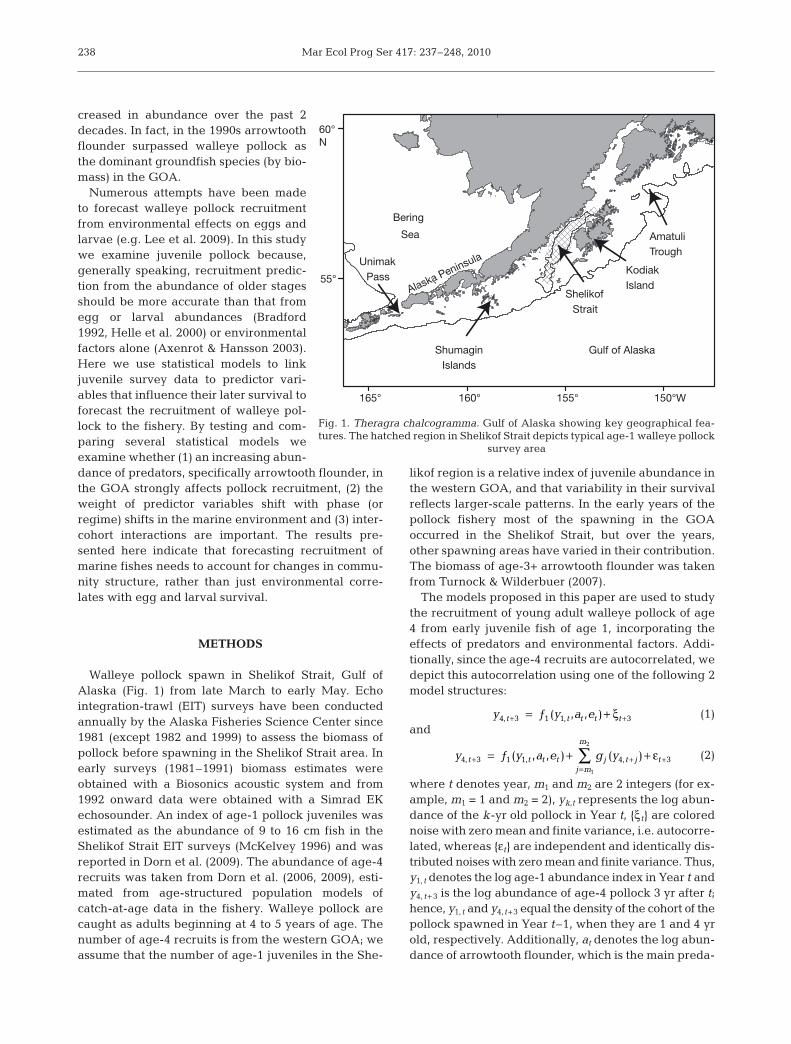
Walleye pollock spawn in Shelikof Strait, Gulf ofAlaska (Fig. 1) from late March to early May. Echointegration-trawl (EIT) surveys have been conductedannually by the Alaska Fisheries Science Center since1981 (except 1982 and 1999) to assess the biomass ofpollock before spawning in the Shelikof Strait area. Inearly surveys (1981–1991) biomass estimates wereobtained with a Biosonics acoustic system and from1992 onward data were obtained with a Simrad EKechosounder. An index of age-1 pollock juveniles wasestimated as the abundance of 9 to 16 cm fish in theShelikof Strait EIT surveys (McKelvey 1996) and wasreported in Dorn et al. (2009). The abundance of age-4recruits was taken from Dorn et al. (2006, 2009), esti-mated from age-structured population models ofcatch-at-age data in the fishery. Walleye pollock arecaught as adults beginning at 4 to 5 years of age. Thenumber of age-4 recruits is from the western GOA; weassume that the number of age-1 juveniles in the She-

likof region is a relative index of juvenile abundance inthe western GOA, and that variability in their survivalreflects larger-scale patterns. In the early years of thepollock fishery most of the spawning in the GOAoccurred in the Shelikof Strait, but over the years,other spawning areas have varied in their contribution.The biomass of age-3+ arrowtooth flounder was takenfrom Turnock & Wilderbuer (2007).

The models proposed in this paper are used to studythe recruitment of young adult walleye pollock of age4 from early juvenile fish of age 1, incorporating theeffects of predators and environmental factors. Addi-tionally, since the age-4 recruits are autocorrelated, wedepict this autocorrelation using one of the following 2model structures:

(1)and

(2)

where t denotes year, m1 and m2 are 2 integers (for ex-ample, m1 = 1 and m2 = 2), yk,t represents the log abun-dance of the k-yr old pollock in Year t, {ξt} are colorednoise with zero mean and finite variance, i.e. autocorre-lated, whereas {εt} are independent and identically dis-tributed noises with zero mean and finite variance. Thus,y1, t denotes the log age-1 abundance index in Year t andy4, t+3 is the log abundance of age-4 pollock 3 yr after t;hence, y1,t and y4,t+3 equal the density of the cohort of thepollock spawned in Year t–1, when they are 1 and 4 yrold, respectively. Additionally, at denotes the log abun-dance of arrowtooth flounder, which is the main preda-

y y a e g yt t t t j t jj m

m

t4 3 1 1 4 3

1

2

, , ,ƒ ( , , ) ( )+ +=

+= + +∑ ε

y y a et t t t t4 3 1 1 3, ,ƒ ( , , )+ += + ξ

238

150°W155°160°165°

60°N

55°

Shelikof

Strait

Bering

Sea

Gulf of AlaskaShumagin

Islands

Amatuli

TroughUnimak

PassKodiak

IslandAlaska Peninsula

Fig. 1. Theragra chalcogramma. Gulf of Alaska showing key geographical fea-tures. The hatched region in Shelikof Strait depicts typical age-1 walleye pollock

survey area

Zhang et al.: Pollock recruitment forecast models

tor of the juvenile pollock in the western GOA, and et

represents a vector of environmental factors in year t,which includes the spring sea surface temperature (SST,i.e. the average SST from April to June), the fall SST (theaverage SST from July to September), the spring sea sur-face wind speed, the fall wind speed and the mean an-nual wind speed. The SST variables were derived fromaverage monthly SST interpolated across a longitudeband in the GOA from 155.6° W to 157.5° W and cen-tered at latitude 56.2° N (data source: A. Macklin, PacificMarine Environmental Laboratory pers. comm., www.cdc.noaa.gov/cdc/reanalysis/). The wind speed covari-ates were computed from sea level pressure data col-lected twice per day in Shelikof Strait (56° N, 156° W)(data source: A. Macklin & M. Spillane, Pacific MarineEnvironmental Laboratory pers. comm.). The termƒ1(y1, t,at,et) summarizes the main effects on the recruit-ment of age-4 pollock. We tried several systems of nota-tion and the preceding format was easiest to follow. Anotation system formed around pollock year classes wascomplicated because of the 2 time sequences for pollockand arrowtooth flounder, and it was difficult to use pol-lock year class to indicate the time subscript of the floun-der. In the model comparison and selection, we em-ployed Akaike’s information criterion (AIC) for modelcomparison and selection. We also used model diagnos-tic checks such as the residuals’ normality test, constantvariance and autocorrelation checks among the residu-als (ACF and Ljung-Box tests) (see Chapter 8 in Cryer &Chan 2008) and outlier detection methods.

For Model (1), any autocorrelation in the age-4recruits beyond that induced by the main regressioneffects ƒ1(y1, t,at,et) is modeled by the autocorrelatederror, {ξt+3}, which, in practice, is specified as someautoregressive (AR) error process. On the other hand,Model (2) uses the lagged recruitment (y4, t+j, j = 2,1,0)to account for any such autocorrelation in the recruit-ment data. Below, we refer to the autocorrelation in therecruitment beyond that induced by the main effectsƒ1(y1, t,at,et) as the extra autocorrelation. Because theresponse variable, y4, t+3, is the recruitment of age-4pollock in Year t+3, its lag-1, i.e. the recruitment ofage-4 in the previous year, equals y4, t+ 2. Similarly, y4, t+j

in the term gj (y4, t+j) is the lag-(3–j) recruitment.The autocorrelation patterns in the recruitment mod-

els may result from intercohort interactions in the wall-eye pollock population. Specifically, we demonstrate 3such mechanisms in the simple case of linear andnoise-free dynamics. One mechanism results in the ARerror process as specified in Model (1), and the other 2mechanisms introduce different lagged recruitmentinto Model (2).

First, the autocorrelation structure in Model (1) canbe justified by cannibalism and/or competition fromadult pollock, specified as the age-4+ (age 4 and older)

group, in which case the (linear) recruitment dynamicsis driven by the following system of equations:

(3a)

(3b)

(3c)

Eq. (3a) models the recruitment from age-1 pollock toage 4; the term β1at models the effects of the arrowtoothflounder on the recruitment and ωy4+,t represent the ef-fects of cannibalism of the age-4+ group on the juvenilepollock and/or competition effects from the older pol-lock in the recruitment process. It is expected that ω isnegative. (We generally use greek letters to denote un-known model parameters to be estimated from thedata.) Eq. (3b) accounts for the survival of the age-4+group from the previous year given by δy4+,t and newmembers from the age-3 group represented by y4y3,t.Eq. (3c) accounts for the survival of age-2 fish to age 3given by y3y2,t and competition from age-4+ pollockmodeled by τ3y4+,t. Note that the γ’s are expected to bebetween 0 and 1, and so is δ. Eq. (3a) is a special case ofEq. (1) where ƒ1 is a linear function and the error termξt + 3 equals ωy4+,t, which we now show to be an autore-gressive process; hence, the error term in Eq. (1) is au-tocorrelated. Indeed, Eqs. (3b) & (3c) imply that:

(3d)

Since the γ’s are expected to be between 0 and 1, thecoefficient γ4γ3 is probably negligible; therefore, thepreceding equation can be approximated by:

(3e)

In practice, the preceding relationship holds only onthe average, so that a stochastic error term has to beadded to the right side of the equation; hence, {y4+,t} isapproximately an AR(2) process, with δ being theAR(1) coefficient and γ4τ3 being the AR(2) coefficient.In particular, δ can be interpreted as the survival rateof the age-4+ pollock. The interpretation of the AR(2)coefficient estimate is more complex as it equals theproduct γ4τ3, which is expected to be negative becauseof the assumed positivity of γ4 and the negativity of τ3.As for Model (2), the extra autocorrelation is assumed tobe captured by the lagged recruits. Such an autocorre-lation structure can be attributed to interactions be-tween the young adult pollock (age 4) and the juvenilepollock, in which case the walleye pollock populationdynamics follow the following system of equations:

(4a)

(4b)

(4c)

(4d)a a yt t t+ = +1 1ϕ ϑ ,

y a y yt t t t2 1 0 2 1 2 2 2 1 2 4, , , , , ,+ = + + +β β β τ

y a y yt t t t3 2 0 3 1 3 1 2 3 2 1 3 4 1, , , , , ,+ + + += + + +β β β τ

y y yt t t4 3 0 4 2 4 3 2 4 4 2, , , , ,+ + += + +β β τ*

y y yt t t4 1 4 4 3 4 1+ + + + −= +, , ,δ γ τ

y y y yt t t t4 1 4 4 3 4 1 4 3 2 1+ + + + − −= + +, , , ,δ γ τ γ γ

y y yt t t3 1 3 2 3 4, , ,+ += +γ τ

y y yt t t4 1 4 3 4+ + += +, , ,γ δ

y a y yt t t t4 3 0 1 2 1 4, , ,+ += + + +β β β ω

239

Mar Ecol Prog Ser 417: 237–248, 2010

Eq. (4a) shows the recruiting process of age-4 wall-eye pollock from age 3, which includes the survival ofage-3 fish given by β2,4y3,t+ 2 and the interactionsbetween the age-4 pollock and the age-3 fish in yeart+2 in terms of τ*

4,y4,t+ 2. The coefficient τ*

4 reflects theintergroup interactions in 2 aspects: (1) it measures thecompetition and/or cannibalism between age-4 andage-3 pollock, and (2) it accounts for misclassificationbetween the age-4 group and its neighboring agegroups, which commonly occurs when a certain por-tion of a strong year class are incorrectly aged andoverflow into adjacent year classes. The competitionand/or cannibalistic effects tend to reduce the recruit-ment of age-4 pollock, and misclassification probablyresults in a positive association between the age-4recruitment and its lag-1. Since these 2 interactions areopposite in direction, the sign of τ*

4 is undetermined inEq. (4a), which is also the reason for adding an asteriskto this coefficient. Eq. (4b) accounts for the survival ofage-3 pollock from the previous year’s age-2 fish in theterm β2,3y2,t+1, the predation from arrowtooth flounderrepresented by β1,3at+1 and the competition and/orcannibalism between the age-4 and age-2 pollockdenoted by τ3y4,t+1. In Eq. (4b), τ3 is expected to be <0,because it mainly assesses the intergroup competitionand/or cannibalism. Similarly, the coefficient τ2 in Eq.(4c) is expected to be negative. Eq. (4d) indicates thatthe abundance of the flounder predators is related totheir last year’s abundance and the corresponding age-1 pollock abundance, as arrowtooth flounder mainlyeats age-0 and age-1 pollock, as well as some age-2fish. The coefficients ϕ and υ are expected to be posi-tive. Substituting Eqs. (4b–d) into Eq. (4a) yields:

(4e)

The model represented by Eq. (4e) contains the lag-1to lag-3 of the recruitment that generates the extra au-tocorrelation in the recruits of age-4 walleye pollock.The parameters β2,j, j = 2,3,4 are survival rates that arelikely to fall between 0 and 1. If we further assumeweak competition and/or cannibalism between theage-4 and the age-1 pollock (small τ2 in magnitude),the coefficient of y4,t in Eq. (4e) is negligible comparedwith the coefficients of y4,t+ 2 and y4,t+1. Therefore, therecruitment equation can be simplified as:

(4f)

The terms within the square brackets of Eq. (4f) mea-sures the lagged recruitment effects on the recruit-ment of age-4 pollock. Since the sign of the parameterτ*

4 is unclear, we cannot determine the sign of the lag-1

recruitment effect. However, we expect a negative lag-2 effect in the recruiting model with the negative τ3

and positive β2,4. We can further generalize Eq. (4f) byreplacing the linear lagged recruitment by nonlinearlag-1 and lag-2 effects in terms of gj(y4,t +j), j = 1,2. Sim-ilarly, we constructed a mechanistic model that resultsin explaining the extra autocorrelation in terms of thelag-2 and lag-3 recruitment effects. However, as thatmodel is discredited by the data (see ‘Results’), for sim-plicity we do not elaborate on the third model.

Although we mainly assume linear effects in theabove derivation, the models may be rendered moreflexible by allowing nonlinear effects in terms of someunknown smooth functions and by including stochasticerrors in the models. Indeed, these models then fallinto the general framework of the generalized additivemixed models (GAMMs) (Lin & Zhang 1999, Wood2006). The recruitment models in the form of Eqs. (1) &(2) can be represented as a GAMM. For the simplecase of single covariate and Gaussian errors, theGAMM takes the following form:

(5)

where the response wt bears a nonlinear relationshipwith the covariate ut and the noise terms {ξt} are auto-correlated. For the simple case that {ξt} has a multivari-ate normal distribution with zero mean vector and co-variance matrix Λ, the log-likelihood of model (5) isgiven by –0.5 × log⏐Λ⏐–{W– s(U)}’Λ–1–{W–s (U)}/2, upto some additive constant, where W is the vector of re-sponse values, s(U) the vector of the smooth function sevaluated at the covariate values, ⏐Λ⏐ is the determi-nant of the covariance matrix Λ. For estimating the un-known smooth function, we use the penalized likeli-hood approach, which tries to find the function estimatethat provides good fit to the data and yet assures thatthe function is not too rough. The penalty term is a mul-tiple of the integrated squared second derivative of thesmooth function, i.e. λ∫{s (u)}2du where the non-nega-tive parameter λ is known as the smoothing parameterthat describes the trade-off between goodness of fit andsmoothness of the function estimate, and s denotes thesecond derivate of s. Altogether, the GAMM can be es-timated by maximizing the penalized log-likelihood:–0.5 × log⏐Λ⏐–{W– s(U)}’Λ–1–{W– s (U)}/2 – λ∫{s (u)}2du.

It should be noted that if the noise terms are uncorre-lated over time, then the GAMM becomes the general-ized additive model (GAM); see Wood (2006) fordetails and other estimation methods.

Since a threshold structure was introduced for fittingthe main effects in ƒ1(y1, t,at,et), we needed to develop atest for the validity of the proposed threshold structure.Considering a possible shift of the arrowtooth flounderspatial distribution from the late 1980s to early 1990sand the occurrence of an environmental regime shift

w s u t nt t t= + =( ) , , ,...ξ 1 2

y a y y yt t t t t4 3 0 1 2 1 4 4 2 2 4 3 4 1, , , , ,[ ]+ + += + + + +β β β τ β τ*

y t4 3 0 4 2 4 0 3 2 4 2 3 0 2 2 4 1 3, , , , , , , , ,[ ] [+ = + + + +β β β β β β β β ϕ ββ β β

β β ϑ β β β2 4 2 3 1 2

2 4 1 3 2 4 2 3 2 2 1

, , ,

, , , , , ,

]

[ ] [

a

y

t

t+ + + ττ β τ β β τ

β β4 4 2 2 4 3 4 1 2 4 2 3 2 4

0 1

*y y y

a

t t t

t

, , , , , , ]+ ++ +

= + ++ + + ++ +β τ β τ β β τ2 1 4 4 2 2 4 3 4 1 2 4 2 3 2 4y y y yt t t t, , , , , , ,[ * ]]

240

Zhang et al.: Pollock recruitment forecast models

about the same time (see below), we further proposeddifferent arrowtooth flounder predation effects beforeand after a threshold year during that period. A thresh-old year effect in the models was assessed by testingthe null hypothesis (H0) that the arrowtooth flounderpredation effect was present for all years versus thealternative hypothesis (Ha) that it started to becomeimportant to walleye pollock survival after a thresholdyear. A likelihood ratio test was employed to justify thethreshold structure in arrowtooth flounder predation.Let θ be the parameter vector, including the thresholdyear, logL(θ0,n) be the log-likelihood function evalu-ated at the maximum likelihood estimators under thenull hypothesis, and logL(θn) be the maximum log-like-lihood function under the general hypotheses. The log-likelihood ratio, lr, can be written as lr = logL(θn) –logL(θ0,n), which is used as the test statistic. ForModel (1) with stochastic error process, the empiricaldistribution of the test statistic under the null hypothe-sis is obtained by the following bootstrap approach.Based on the residual vector (ξ) and the correlationmatrix (Λ) estimated under the null hypothesis, we

calculate the normalized residuals, ε = Λ–1/2 ξ0. For each k = 1, … K, we randomly permute the elements in

ε0 to get ε0(k). Using the parameter estimator θ0,n and the

residuals ξ0(k) = Λ–1/2 ε0

(k), we generate the new recruit-

ment level data . Based

on the generated data, y4,t+ 3(k), we calculate lr (k).

The empirical distribution of the test statistic is formedfrom the lr (k) values. Additionally, to form such anempirical distribution based on Model (2), whose errorterms are independent and identically distributed, wecan generate the new data by bootstrapping the resid-uals directly. Finally, the p-value of the likelihood ratiotest is calculated as the proportion of lr (k) values thatare higher than the observed lr .

RESULTS

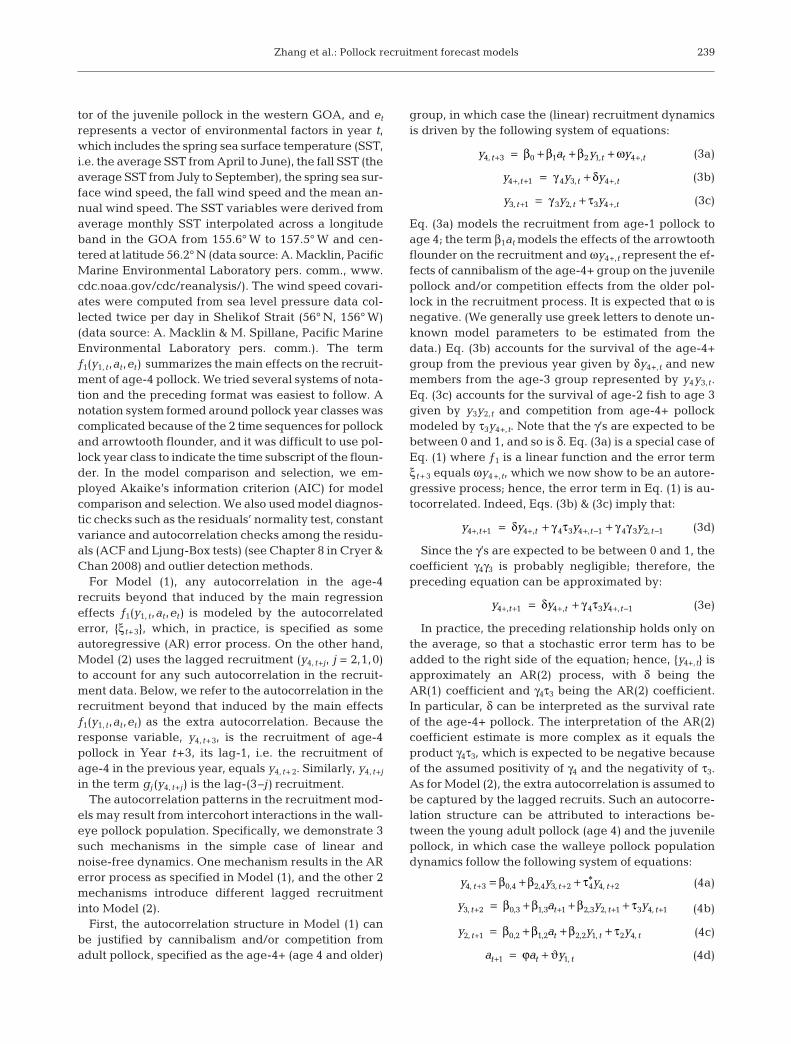
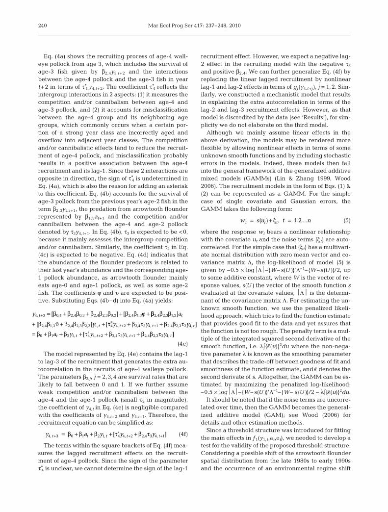
There was generally a positive relationship betweenthe age-1 abundance index and the recruitment ofwalleye pollock to the fishery 3 yr later (Fig. 2). How-ever, the relationship appeared to have shifted down-ward after 1991, suggesting the presence of emergingfactors on age-1 pollock survival. At around the sametime, arrowtooth flounder abundance was increasingand surpassed pollock to become the dominantgroundfish species in the GOA (Fig. 3). We thereforeselected these factors (age-1 pollock abundance,arrowtooth flounder abundance, a threshold effect)and some environmental factors (e.g. temperature) totest and compare in the statistical recruitment predic-tion models.

In the ‘Methods’, we discussed 3 mechanisms toderive the autocorrelation structures in recruitmentmodels. For each of the 3 autocorrelation structures,we selected one fitted model based on AIC and per-formed model diagnostic results. As shown in Table 1,the selected model with the AR(2) error process has aslightly better AIC score (22.5) and adjusted R2 (81.5%)than the model including lag-1 and lag-2 recruitmenteffects, with AIC = 24.0 and adjusted R2 = 80.7%; themodel-fitting results from both models are discussed indetail below. The AIC of the model containing lag-2and lag-3 recruitment (28.3) is much higher than theAICs from the other 2 selected models (Table 1), whichindicates that this model is discredited by the data.Temperature was not significant in any of the modelsand was dropped from consideration. Including springSST as an additive covariate results in an increase inthe AIC for each of the 3 models reported in Table 1,

ˆ ƒ ( , , ) ˆ,

( ), ˆ , ( ),

(

,y y a et

kt t t t

k

n4 3 1 1 3 00+ += +θ ξ ))

241

−6 −4 −2 0

21.0

20.5

20.0

19.5

19.0

18.5

18.0

17.5

2

Log age-1 abundance index

Lo

g a

ge-4

recru

itm

en

t

Fig. 2. Theragra chalcogramma. Scatter plot of (log) cohort-specific age-1 walleye pollock abundance versus (log) age-4recruitment. (s) observations before 1992; (J) observations

since 1992

1980 1985 1990 1995 2000 2005

Year

Lo

g b

iom

ass (p

ollo

ck a

nd

AT

F)

15.5

15.0

14.5

14.0

13.5

13.0

Fig. 3. Theragra chalcogramma. Time plot of (log) walleyepollock biomass and (log) arrowtooth flounder biomass. (s)

(log) biomass of age 3+ pollock; (J) (log) flounder biomass

Mar Ecol Prog Ser 417: 237–248, 2010

e.g. an increase in AIC from 22.5 to 24.2 for Model (6)with AR(2) error structure; similarly, other environ-mental factors, including fall SST and various windspeeds, were found to be inconsequential. We also fit-ted Model (6) with SST as the threshold variable, butthat fitted model was deemed unacceptable based onmodel diagnostics and interpretation. Consequently,we shall confine our discussion to the first 2 models.

The first fitted model contains an autocorrelatederror process {ξt}. Fitting results with different autore-gressive structures in {ξt} suggested that an AR(2) errorprocess provided the best fit for the data with the low-est AIC values (Table 2). The mechanism for this AR(2)error process is shown by Eqs. (3a)–(3c). A preliminaryanalysis indicated that the log age-1 abundance (y1,t)and log arrowtooth flounder abundance (at) after thethreshold year (tc) were linearly correlated with therecruitment level (y4,t+ 3). Additionally, no environmen-tal factors enter into the model, probably because anychange in environmental factors that strongly influ-enced juvenile survival was incorporated in the thresh-old shift term. Therefore, the fitted model with theAR(2) error process has the following structure:

(6)

where the dummy variable 1(t>tc) equals 1 in the yearsafter the threshold year tc, and 0 otherwise, so β1at1(t>tc)

accounts for the threshold arrowtooth flounder preda-

tion effect on pollock recruitment after year tc. Theerrors form a stationary Gaussian AR(2) process:

, where φ1 and φ2 are the autore-gressive parameters and the εt are independent andidentically normally distributed errors, so that

follows a multivariate normaldistribution N(0,σ2Λ), where (t0+3) and (tL+3) denotethe first and last recruiting years of age-4 pollock in thestudy period, respectively, and Λ is the correlationmatrix with an AR(2) structure. More specifically, ρj =φ1ρj–1 + φ2ρj–2, j ≥ 2, where ρj is the correlation betweenξt and ξt–j, with the initial conditions ρ0 = 1, ρ1 = φ1/(1 – φ2) and σ2 is the stationary variance of ξt.

To check whether the threshold structure of thearrowtooth flounder predation effect in Model (6) wasappropriate for the data, we employed the likelihoodratio test discussed in the ‘Methods’. The p-value of thelikelihood ratio test for the threshold structure inModel (6) is 0.024. Thus, there is strong evidence thatthe flounder predation affected pollock recruitmentafter a threshold year tc.

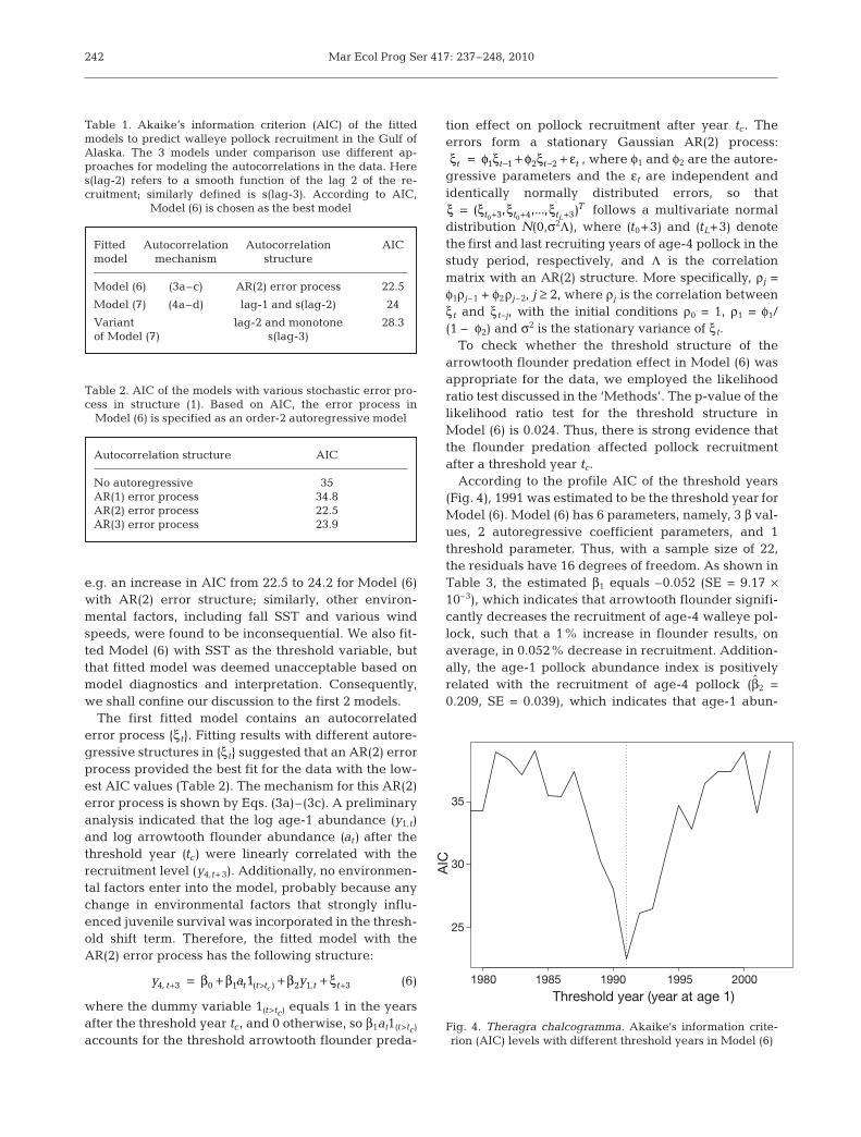
According to the profile AIC of the threshold years(Fig. 4), 1991 was estimated to be the threshold year forModel (6). Model (6) has 6 parameters, namely, 3 β val-ues, 2 autoregressive coefficient parameters, and 1threshold parameter. Thus, with a sample size of 22,the residuals have 16 degrees of freedom. As shown inTable 3, the estimated β1 equals –0.052 (SE = 9.17 ×10–3), which indicates that arrowtooth flounder signifi-cantly decreases the recruitment of age-4 walleye pol-lock, such that a 1% increase in flounder results, onaverage, in 0.052% decrease in recruitment. Addition-ally, the age-1 pollock abundance index is positivelyrelated with the recruitment of age-4 pollock (β2 =0.209, SE = 0.039), which indicates that age-1 abun-

ξ ξ ξ ξ= + + +( , ,..., )t t tT

L0 03 4 3

ξ φ ξ φ ξ εt t t t= + +− −1 1 2 2

y a yt t t t t tc4 3 0 1 2 1 31, ( ) ,+ > += + + +β β β ξ

242

Fitted Autocorrelation Autocorrelation AICmodel mechanism structure

Model (6) (3a–c) AR(2) error process 22.5

Model (7) (4a–d) lag-1 and s(lag-2) 24

Variant lag-2 and monotone 28.3of Model (7) s(lag-3)

Table 1. Akaike’s information criterion (AIC) of the fittedmodels to predict walleye pollock recruitment in the Gulf ofAlaska. The 3 models under comparison use different ap-proaches for modeling the autocorrelations in the data. Heres(lag-2) refers to a smooth function of the lag 2 of the re-cruitment; similarly defined is s(lag-3). According to AIC,

Model (6) is chosen as the best model

Autocorrelation structure AIC

No autoregressive 35AR(1) error process 34.8AR(2) error process 22.5AR(3) error process 23.9

Table 2. AIC of the models with various stochastic error pro-cess in structure (1). Based on AIC, the error process in

Model (6) is specified as an order-2 autoregressive model

Threshold year (year at age 1)

AIC

1980

35

30

25

1985 1990 1995 2000

Fig. 4. Theragra chalcogramma. Akaike’s information crite-rion (AIC) levels with different threshold years in Model (6)

Zhang et al.: Pollock recruitment forecast models

dance is an important factor explaining the variabilityin the recruitment of age-4 pollock.

Based on the estimated autoregressive parameters,φ1 = 0.546 and φ2 = –0.719 (Table 3), the error process{ξt} is, indeed, stationary (see Cryer & Chan 2008,

p. 72). The average length of the stochastic cycle,, is approximately 5 yr (Fig. 5).

The competition and cannibalism between the cohortsof different ages, especially the cannibalism of theadult pollock on the juveniles as detailed inEqs. (3a)–(3c), are instrumental for the 5 yr quasi-periodicity. Additionally, according to the discussion ofthe stochastic mechanism for this model in the previ-ous section, the AR(1) parameter φ1 can be interpretedas the average survival rate of pollock of ages 4+,which is estimated to be 0.546 (= 54.6%), althoughwith considerable uncertainty as the 95% confidenceinterval ranges from 28.5 to 63.5%.

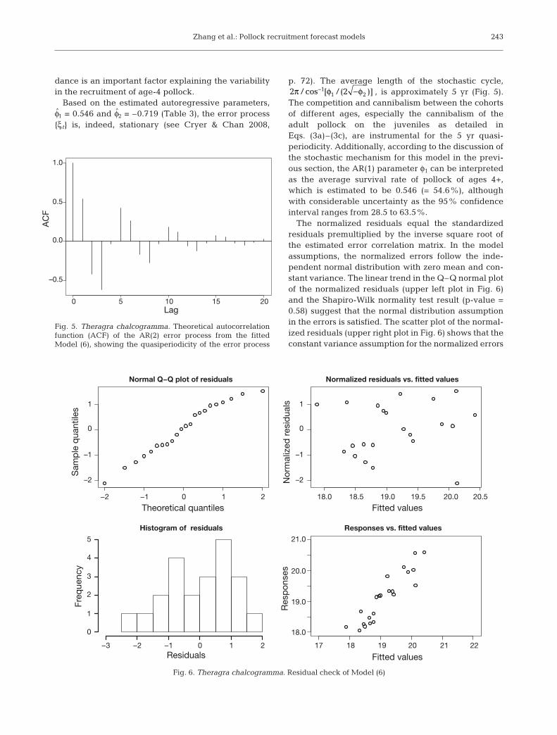
The normalized residuals equal the standardizedresiduals premultiplied by the inverse square root ofthe estimated error correlation matrix. In the modelassumptions, the normalized errors follow the inde-pendent normal distribution with zero mean and con-stant variance. The linear trend in the Q–Q normal plotof the normalized residuals (upper left plot in Fig. 6)and the Shapiro-Wilk normality test result (p-value =0.58) suggest that the normal distribution assumptionin the errors is satisfied. The scatter plot of the normal-ized residuals (upper right plot in Fig. 6) shows that theconstant variance assumption for the normalized errors

2 211 2π φ φ/ cos [ / ( )]− −

243

Lag

AC

F

0 5 10 15

1.0

0.5

0.0

–0.5

20

Fig. 5. Theragra chalcogramma. Theoretical autocorrelationfunction (ACF) of the AR(2) error process from the fitted Model (6), showing the quasiperiodicity of the error process

−2 −1 0

1

0

–1

–2

1

0

–1

–2

1 2

Normal Q−Q plot of residuals

Theoretical quantiles

Sam

ple

qu

an

tile

s

18.0 18.5 19.0 19.5 20.0 20.5

Normalized residuals vs. fitted values

Fitted values

No

rmaliz

ed

resid

uals

Histogram of residuals

Residuals

Fre

quency

5

4

3

2

1

0

17

21.0

20.0

19.0

18.0

18 19 20 21 22

Responses vs. fitted values

Fitted values

Resp

onses

−2−3 −1 0 1 2

Fig. 6. Theragra chalcogramma. Residual check of Model (6)

Mar Ecol Prog Ser 417: 237–248, 2010

appears appropriate. The normalized residuals appearto be uncorrelated over time, which is supported by theACF and Ljung-Box test. Therefore, the assumptions ofthe error terms are satisfied approximately for the fit-ted Model (6), suggesting that it provides a good fit tothe data.

Owing to the AR(2) correlation structure in the errorterm, {ξt} and that the covariates in Model (6) lagthe recruitment by 3 yr, we can compute out-of-samplek years ahead forecasts for k = 1, 2 and 3 yr into thefuture by the following formula:

where n is the last year of the study period, being 2006,and ξ n+k are computed recursively by the formula:

with being the re-gression residuals from Model (6) for t ≤ n. For formu-lae to compute 95% prediction intervals see Chapter 9in Cryer & Chan (2008). For computing forecasts for4 yr or longer, we needed to compute out-of-sampleforecasts for arrowtooth flounder abundance and thatof 1 yr old walleye pollock, which required the devel-opment of joint modeling for these covariate processeswith the recruitment. Note that y1,t in year 1999 was amissing value, and we used the naïve scheme ofaveraging the y1, t values in 1998 and 2000 to imput thismissing log age-1 abundance index. The fitted re-cruitment of age-4 pollock in 2002 was calculatedbased on the imputed age-1 abundance in 1999.

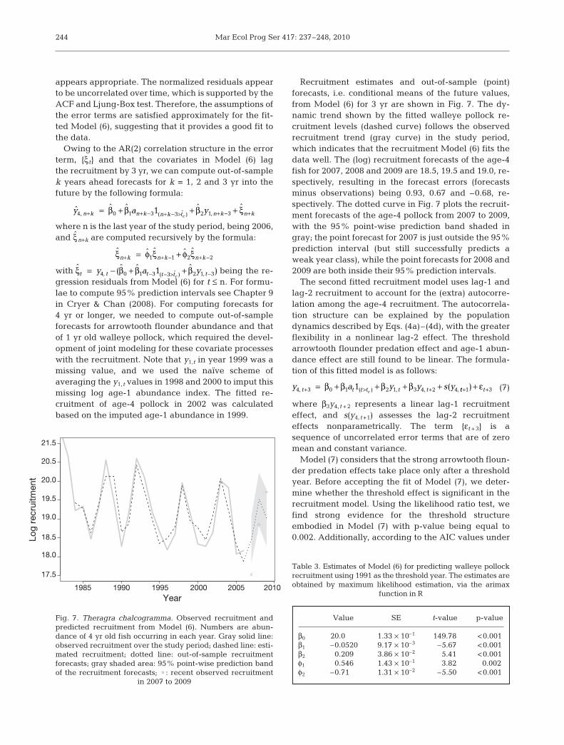
Recruitment estimates and out-of-sample (point)forecasts, i.e. conditional means of the future values,from Model (6) for 3 yr are shown in Fig. 7. The dy-namic trend shown by the fitted walleye pollock re-cruitment levels (dashed curve) follows the observedrecruitment trend (gray curve) in the study period,which indicates that the recruitment Model (6) fits thedata well. The (log) recruitment forecasts of the age-4fish for 2007, 2008 and 2009 are 18.5, 19.5 and 19.0, re-spectively, resulting in the forecast errors (forecastsminus observations) being 0.93, 0.67 and –0.68, re-spectively. The dotted curve in Fig. 7 plots the recruit-ment forecasts of the age-4 pollock from 2007 to 2009,with the 95% point-wise prediction band shaded ingray; the point forecast for 2007 is just outside the 95%prediction interval (but still successfully predicts aweak year class), while the point forecasts for 2008 and2009 are both inside their 95% prediction intervals.

The second fitted recruitment model uses lag-1 andlag-2 recruitment to account for the (extra) autocorre-lation among the age-4 recruitment. The autocorrela-tion structure can be explained by the populationdynamics described by Eqs. (4a)–(4d), with the greaterflexibility in a nonlinear lag-2 effect. The thresholdarrowtooth flounder predation effect and age-1 abun-dance effect are still found to be linear. The formula-tion of this fitted model is as follows:

(7)

where β3y4, t + 2 represents a linear lag-1 recruitmenteffect, and s(y4, t +1) assesses the lag-2 recruitmenteffects nonparametrically. The term {εt + 3} is asequence of uncorrelated error terms that are of zeromean and constant variance.

Model (7) considers that the strong arrowtooth floun-der predation effects take place only after a thresholdyear. Before accepting the fit of Model (7), we deter-mine whether the threshold effect is significant in therecruitment model. Using the likelihood ratio test, wefind strong evidence for the threshold structureembodied in Model (7) with p-value being equal to0.002. Additionally, according to the AIC values under

y a y y s yt t t t t tc4 3 0 1 2 1 3 4 2 41, ( ) , , ,(+ > += + + + +β β β β tt t+ ++1 3) ε

ˆ ( ˆ ˆ ˆ ), ( ˆ ) ,ξ β β βt t t t t ty a yc

= − + +− − > −4 0 1 3 3 2 1 31

ˆ ˆ ˆ ˆ ˆξ φ ξ φ ξn k n k n k+ + − + −= +1 1 2 2

ˆ ˆ ˆ ˆ, ( ˆ ) ,y a yn k n k n k t n kc4 0 1 3 3 2 11+ + − + − > += + +β β β −− ++3 ξn k

244

1985 1990

20.5

20.0

19.5

19.0

18.5

18.0

17.5

21.5

1995 2000 2005 2010

Year

Lo

g r

ecru

itm

en

t

Fig. 7. Theragra chalcogramma. Observed recruitment andpredicted recruitment from Model (6). Numbers are abun-dance of 4 yr old fish occurring in each year. Gray solid line:observed recruitment over the study period; dashed line: esti-mated recruitment; dotted line: out-of-sample recruitmentforecasts; gray shaded area: 95% point-wise prediction bandof the recruitment forecasts; : recent observed recruitment

in 2007 to 2009

Value SE t-value p-value

β0 20.0 1.33 × 10–1 149.78 <0.001β1 –0.0520 9.17 × 10–3 –5.67 <0.001β2 0.209 3.86 × 10–2 5.41 <0.001φ1 0.546 1.43 × 10–1 3.82 0.002φ2 –0.71 1.31 × 10–2 –5.50 <0.001

Table 3. Estimates of Model (6) for predicting walleye pollockrecruitment using 1991 as the threshold year. The estimates areobtained by maximum likelihood estimation, via the arimax

function in R

Zhang et al.: Pollock recruitment forecast models

different threshold choices, the estimated thresholdyear is 1991.

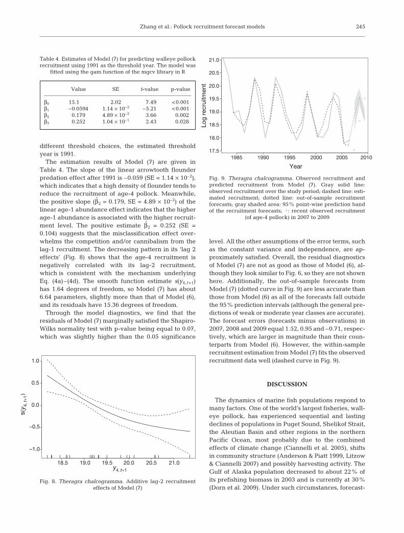
The estimation results of Model (7) are given inTable 4. The slope of the linear arrowtooth flounderpredation effect after 1991 is –0.059 (SE = 1.14 × 10–2),which indicates that a high density of flounder tends toreduce the recruitment of age-4 pollock. Meanwhile,the positive slope (β2 = 0.179, SE = 4.89 × 10–2) of thelinear age-1 abundance effect indicates that the higherage-1 abundance is associated with the higher recruit-ment level. The positive estimate β2 = 0.252 (SE =0.104) suggests that the misclassification effect over-whelms the competition and/or cannibalism from thelag-1 recruitment. The decreasing pattern in its ‘lag 2effects’ (Fig. 8) shows that the age-4 recruitment isnegatively correlated with its lag-2 recruitment,which is consistent with the mechanism underlyingEq. (4a)–(4d). The smooth function estimate s(y4, t +1)has 1.64 degrees of freedom, so Model (7) has about6.64 parameters, slightly more than that of Model (6),and its residuals have 15.36 degrees of freedom.

Through the model diagnostics, we find that theresiduals of Model (7) marginally satisfied the Shapiro-Wilks normality test with p-value being equal to 0.07,which was slightly higher than the 0.05 significance

level. All the other assumptions of the error terms, suchas the constant variance and independence, are ap-proximately satisfied. Overall, the residual diagnosticsof Model (7) are not as good as those of Model (6), al-though they look similar to Fig. 6, so they are not shownhere. Additionally, the out-of-sample forecasts fromModel (7) (dotted curve in Fig. 9) are less accurate thanthose from Model (6) as all of the forecasts fall outsidethe 95% prediction intervals (although the general pre-dictions of weak or moderate year classes are accurate).The forecast errors (forecasts minus observations) in2007, 2008 and 2009 equal 1.52, 0.95 and –0.71, respec-tively, which are larger in magnitude than their coun-terparts from Model (6). However, the within-samplerecruitment estimation from Model (7) fits the observedrecruitment data well (dashed curve in Fig. 9).

DISCUSSION

The dynamics of marine fish populations respond tomany factors. One of the world’s largest fisheries, wall-eye pollock, has experienced sequential and lastingdeclines of populations in Puget Sound, Shelikof Strait,the Aleutian Basin and other regions in the northernPacific Ocean, most probably due to the combinedeffects of climate change (Ciannelli et al. 2005), shiftsin community structure (Anderson & Piatt 1999, Litzow& Ciannelli 2007) and possibly harvesting activity. TheGulf of Alaska population decreased to about 22% ofits prefishing biomass in 2003 and is currently at 30%(Dorn et al. 2009). Under such circumstances, forecast-

245

Value SE t-value p-value

β0 15.1000 2.02 7.49 <0.001β1 –0.0594 1.14 × 10–2 –5.21 <0.001β2 0.179 4.89 × 10–2 3.66 0.002β3 0.252 1.04 × 10–1 2.43 0.028

Table 4. Estimates of Model (7) for predicting walleye pollockrecruitment using 1991 as the threshold year. The model was

fitted using the gam function of the mgcv library in R

18.5

1.0

0.5

0.0

–0.5

–1.0

19.0 19.5 20.0 20.5 21.0y4, t+1

s(y

4, t

+1)

Fig. 8. Theragra chalcogramma. Additive lag-2 recruitment effects of Model (7)

1985 1990 1995 2000 2005 2010

Year

20.5

20.0

19.5

19.0

18.5

18.0

17.5

21.0

Lo

g r

ecru

itm

ent

Fig. 9. Theragra chalcogramma. Observed recruitment andpredicted recruitment from Model (7). Gray solid line:observed recruitment over the study period; dashed line: esti-mated recruitment; dotted line: out-of-sample recruitmentforecasts; gray shaded area: 95% point-wise prediction bandof the recruitment forecasts; : recent observed recruitment

(of age-4 pollock) in 2007 to 2009

Mar Ecol Prog Ser 417: 237–248, 2010

ing recruitment to the population is important as thecommercial harvest takes increasingly younger mem-bers of the population. The traditional methods of fore-casting marine fisheries recruitment from environmen-tal conditions during egg and larval stages have beenmarginally successful due to the complexity of inter-acting biological and environmental conditions cou-pled with the high and variable mortality of these earlylife history stages (Bailey et al. 2005, Houde 2008),although there are exceptions (Svendsen et al. 2007).Here we demonstrate some novel forecasting modelsthat are fairly successful. In our forecasting models westart with 1 yr old juvenile walleye pollock abundancein survey catches and examine factors that may in-fluence their survival over the next 3 to 4 yr untilrecruitment. We find that a change in the predatorcommunity favoring an increase in the abundance ofarrowtooth flounder (a voracious predator of juvenilepollock that has come to dominate the groundfish bio-mass in the Gulf of Alaska in the past decade, Turnock& Wilderbuer 2007), a strong autocorrelation effectprobably caused by year class interactions and athreshold effect in predation that is linked with a phaseshift in environmental factors are closely coupled withrecruitment predictability. These findings represent anew approach in forecasting recruitment success ofmarine fisheries and further demonstrate the impor-tance of predation during the juvenile stage influenc-ing the dynamics of marine fish populations.

Recruitment of walleye pollock became decoupledfrom larval mortality in the early 1990s and controlshifted to juvenile survival (Bailey 2000); a shift in com-munity structure also occurred around the same timethat included a marked increase in the abundance offlatfishes (Anderson & Piatt 1999), particularly arrow-tooth flounder. In general, larval dynamics are thoughtto activate variability in year class strength, whereaspredation on juveniles is thought to dampen variability(van der Veer 1986, Bailey et al. 2005). However,arrowtooth flounder has become an important force inthe recruitment of pollock, as this flounder is currentlythe dominant groundfish species and predator in theGulf of Alaska ecosystem. Arrowtooth flounder bio-mass dwarfs that of other potential predators, such asPacific cod Gadus macrocephalus, by about an order ofmagnitude (NPFMC 2009). Generally about 40 to 50%of the diet of adult arrowtooth flounder comprises juve-nile walleye pollock although the exact compositionand lengths of fish preyed upon depends on availabil-ity (Yang 1993, Yang et al. 2006, Knoth & Foy 2008).Shifts in community structure resulting in changes inabundance of top predators are recognized to havemajor cascading effects on lower trophic levels (Huntet al. 2002, Frank et al. 2005). We perceive that ifand/or when arrowtooth flounder abundance in the

GOA declines, other predators may become importantfactors in juvenile pollock survival, leading to a fore-casting strategy that includes adaptable models.

A threshold effect on the importance of arrowtoothflounder predation on walleye pollock seems to haveoccurred around the same time that control of pollockrecruitment shifted to juvenile survival. In this senseinclusion of the threshold in the model is consonantwith the known biology. We suggest the possibility thatan increasing arrowtooth flounder population mayhave been conditioned over time to locate predictable‘hotspots’ on age-1 juvenile pollock resulting in aphase transition, or their distribution otherwise ex-panded at that time to overlap more with juvenile pol-lock. Recent studies have shown that whereas age-0pollock distributions are variable from year to year,age-1 (Wilson 2009) and older fish distributions (Shimaet al. 2002) are relatively consistent. Alternatively anenvironmental phase shift occurring around the sametime (i.e. 1989, Hollowed et al. 2001), potentially caus-ing a shift in the overlapping distributions of predatorand prey, could be a factor (Ciannelli et al. 2005). Anenvironmental shift that started around 1989 was asso-ciated with changes in a broad array of biological andclimate factors, including enhanced summer warmingin the coastal waters of the GOA (Hare & Mantua2000). Yet another alternative is that the acoustic gearchanged in 1992, near our threshold year, and this gearchange may have altered the log-transformed data bysome additive constant after 1992, resulting in a jumpin the intercept term; however, this effect cannot pro-duce the piece-wise linear threshold effects describedin Models (6) and (7).

Our initial modeling efforts included an interactioneffect of temperature and arrowtooth flounder abun-dance on walleye pollock recruitment. Although the fi-nal model dropped the temperature interaction, it islikely to be an important consideration in the overlap ofpredators and prey; in our case its precision may havebeen affected by using SST as a proxy for bottom tem-perature (BT). In the Bering Sea arrowtooth flounderavoid cold water (Spencer 2008). In the GOA, there issome support that arrowtooth flounder tend to avoidcold water; for example in colder La Niña years they arefound in warmer areas (Speckman et al. 2005). We sug-gest that in some years arrowtooth flounder may avoidcold water over the shelf, influencing their overlap withjuvenile pollock prey. More studies, better understand-ing of temperature interactions and availability of bot-tom temperature data may indicate whether tempera-ture effects should be included in future models.

The autocorrelation among the walleye pollockrecruits included in our models reflects the pollock’spopulation dynamics, which is difficult to explain but isbiologically plausible. The sometimes cyclic nature of

246

Zhang et al.: Pollock recruitment forecast models

population dynamics is well established (e.g. Kendallet al. 1999, Stenseth et al. 2003). Cyclic variations inrecruitment of marine fishes can occur on many scales,from lunar (Meekan et al. 1993) to decadal and longercycles (Southward et al. 1988, Ravier & Fromentin2001). Marine fish recruitment cycles with a periodapproximating a generation time (4 to 5 yr for walleyepollock) may result from intrapopulation interactions(Bjornstad et al. 1999, Bailey et al. 2003). In the fittedmodels with stochastic error terms, the dynamic cyclemay be due to the competition or cannibalism effectsfrom older pollock groups (Bjornstad et al. 1999). Wall-eye pollock in the Bering Sea are highly cannibalisticand there is a strong seasonality in the process (Dwyeret al. 1987) with up to 50 to 90% of the diet of adults inautumn and winter comprised of juveniles, mainlyage-0 fish. There is also a high degree of cannibalismon age-1 pollock in the eastern Hokkaido Island stockof pollock (Yamamura et al. 2001). In the GOA there islittle published information on seasonal changes in thediet of pollock, but in summer around 10% of the dietof adults consisted of juvenile pollock (Yang 1993,Yang et al. 2006). Competition between year classesand between adults and juveniles is also viable since alarge component of the diet of both age-1 pollock andadults is comprised of copepods and euphausids. Com-petition between year classes is also thought to beimportant in recruitment of pollock off easternHokkaido Island (Shida et al. 2007). Autocorrelation injuvenile survival rates may also be linked to autocorre-lation in environmental variables, such as zooplanktonbiomass in the GOA and/or competitor effects on prey(Brodeur et al. 1996, Shiomoto et al. 1997). Conse-quently, we believe that the autocorrelation in pollockdynamics is important to capture in forecasting mod-els, and a better understanding of this phenomenon isneeded.

The models we propose for walleye pollock recruit-ment forecasting are novel in the sense that they arebased on indices that come after the complex egg andlarval period, starting with survey estimates of age-1juveniles. The models account for changes in commu-nity structure, such as an increasing trend in thepredatory capacity of the community, and for biologi-cal causes of the observed periodicity in recruitment.In the hindcast mode, Model (6) in particular providesa very close fit to observed recruitment levels, and theforecasts for 4 yr old fish recruiting in 2007–2009appear to be relatively accurate. This model, which hasa slightly better fit than Model (7) based on AIC andadjusted R2 as well as model diagnostics, accounts forthe effects of age-1 abundance, the threshold effect ofarrowtooth flounder abundance and autocorrelatederror terms due to as yet unidentified covariates onrecruitment 3 yr later. Furthermore, Model (6) provides

a far superior fit (adjusted R2 = 81.5%) than the simplelinear regression with the log age-1 abundance as theonly covariate (adjusted R2 = 31.2%). Model (7) is morespecific and provided insight to the possible missingcovariates, including potential misclassifying ages ofadult pollock (especially spillover effects of strong yearclasses) and predation/competition interactions amongcohorts. There may be other covariates involving stockstructure and spawning behavior, or competition andcannibalism (and their representation), underlying theAR(2) error structure that are not presently recognized.

LITERATURE CITED

Anderson P, Piatt JF (1999) Community reorganization in theGulf of Alaska following ocean climate regime shift. MarEcol Prog Ser 189:117–123

Axenrot T, Hansson S (2003) Predicting herring recruitmentfrom young-of-the-year densities, spawning stock bio-mass, and climate. Limnol Oceanogr 48:1716–1720

Bailey KM (2000) Shifting control of recruitment of walleyepollock (Theragra chalcogramma) after a major climateand ecosystem change. Mar Ecol Prog Ser 198:215–224

Bailey KM, Ciannelli L, Agostini V (2003) Complexity andconstraints combined in simple models of recruitment. In:Browman HI, Skiftesvik AB (eds) The big fish bang. Proc26th Annu Larval Fish Conf. Institute of Marine Research,Bergen, Norway, p 293–301. Also available at: www.fish-larvae.com/e/BigBang/Bailey.pdf

Bailey KM, Ciannelli L, Bond N, Belgrano A, Stenseth NC(2005) Recruitment of walleye pollock in a complex physi-cal and biological ecosystem. Prog Oceanogr 67:24–42

Bjørnstad ON, Fromentin JM, Stenseth NC, Gjøsætter J(1999) Cycles and trends in cod populations. Proc NatlAcad Sci USA 96:5066–5071

Bradford MJ (1992) Precision of recruitment predictions fromearly life stages of marine fishes. Fish Bull 90:439–453

Brodeur RD, Frost BW, Hare SR, Francis RC, Ingraham WJ(1996) Interannual variations in zooplankton biomass inthe Gulf of Alaska, and covariation with California Cur-rent zooplankton biomass. CCOFI Rep 37:80–98

Ciannelli L, Bailey KM, Stenseth NC, Chan KS, Belgrano A(2005) Climate change causing phase transition of walleyepollock (Theragra chalcogramma) recruitment dynamics.Proc Biol Sci 272:1735–1743

Cryer DJ, Chan KS (2008) Time series analysis with applica-tions in R. Springer Verlag, New York

Dorn M, Aydin K, Barbeaux S, Guttormsen M, Megrey B,Spalinger K, Wilkins M (2006) Stock assessment and fish-ery evaluation report: assessment of walleye pollock in theGulf of Alaska. North Pacific Fishery Management Coun-cil,Anchorage, AK. Also available at: www.afsc.noaa.gov/refm/docs/2006/GOApollock.pdf

Dorn M, Aydin K, Barbeaux S, Guttormsen M, Megrey B,Spalinger K, Wilkins M (2009) Stock assessment and fish-ery evaluation report: Gulf of Alaska walleye pollock.North Pacific Fishery Management Council, Anchorage,AK. Also available at: www.afsc.noaa.gov/REFM/docs/2009/GOApollock.pdf

Dwyer DA, Bailey KM, Livingston PA (1987) Feeding habitsand daily ration of walleye pollock (Theragra chalco-gramma) in the eastern Bering Sea, with special referenceto cannibalism. Can J Fish Aquat Sci 44:1972–1984

247

Mar Ecol Prog Ser 417: 237–248, 2010

Frank KT, Petrie B, Choi JS, Leggett WC (2005) Trophic cas-cades in a formerly cod-dominated ecosystem. Science308:1621–1623

Hare SR, Mantua NJ (2000) Empirical evidence for NorthPacific regime shifts in 1977 and 1989. Prog Oceanogr 47:103–145

Helle K, Bogstad B, Marshall TT, Michalsen K, Ottersen G,Pennington M (2000) An evaluation of recruitment indicesfor Arcto-Norwegian cod (Gadus morhua L.). Fish Res 48:55–67

Hjort J (1914) Fluctuations in the great fisheries of northernEurope, viewed in the light of biological research. RappP-V Reun Conseil Int Explor Mer 20:1–228

Hollowed AB, Hare SR, Wooster WS (2001) Pacific basin cli-mate variability and patterns of Northeast Pacific marinefish production. Prog Oceanogr 49:257–282

Houde ED (2008) Emerging from Hjort’s shadow. J NorthwestAtl Fish Sci 41:53–70

Hunt GL Jr, Stabeno P, Walters G, Sinclair E, Brodeur RD,Napp JM, Bond NA (2002) Climate change and control ofthe southeastern Bering Sea pelagic ecosystem. Deep-SeaRes II 49:5821–5854

Kendall BE, Briggs CJ, Murdoch WW, Turchin P and others(1999) Why do populations cycle? A synthesis of statisticaland mechanistic modeling approaches. Ecology 80:1789–1805

Knoth BA, Foy RJ (2008) Temporal variability in the foodhabits of arrowtooth flounder (Atheresthes stomias) in thewestern Gulf of Alaska. NOAA Tech Memo NMFS-AFSC-184

Lee YW, Megrey BA, Mackin SA (2009) Evaluating the per-formance of Gulf of Alaska walleye pollock (Theragrachalcogramma) recruitment forecasting models using aMonte Carlo resampling strategy. Can J Fish Aquat Sci 66:367–381

Lin X, Zhang D (1999) Inference in generalized additivemixed models using smoothing splines. J R Stat Soc B 61:381–400

Litzow MA, Ciannelli L (2007) Oscillating trophic controlinduces community reorganization in a marine ecosystem.Ecol Lett 10:1124–1134

McKelvey DR (1996) Juvenile pollock distribution and abun-dance in Shelikof Strait. What can we learn from acousticsurvey results? NOAA Tech Rep 126:25–34

Meekan MG, Milicich MJ, Doherty PJ (1993) Larval produc-tion drives temporal patterns of larval supply and recruit-ment of a coral reef damselfish. Mar Ecol Prog Ser 93:217–225

Mukhina NV, Marshall CT, Yaragina NA (2003) Tracking thesignal in year-class strength of northeast Arctic codthrough multiple survey estimates of egg, larval and juve-nile abundance. J Sea Res 50:57–75

NOAA (2008) NOAA 200th visions: ocean research. Available at:celebrating200years.noaa.gov/visions/ocean_research/welcome.html

NPFMC (North Pacific Fishery Management Council) (2009)Stock assessment and fishery evaluation report for thegroundfish resources of the Gulf of Alaska. North PacificFishery Management Council, Anchorage, AK. Also avail-able at: www.afsc.noaa.gov/REFM/Docs/2009/GOASafe.pdf

Ravier C, Fromentin JM (2001) Long-term fluctuations in theeastern Atlantic and Mediterranean bluefin tuna popula-tion. ICES J Mar Sci 58:1299–1317

Shida O, Hamatsu T, Nishimura A, Suzaki A, Yamamoto J,Miyashita K, Sakurai Y (2007) Interannual fluctuations inrecruitment of walleye pollock in the Oyashio regionrelated to environmental changes. Deep-Sea Res II 54:2822–2831

Shima M, Hollowed AB, VanBlaricom GR (2002) Changesover time in the sptial distribution of walleye pollock(Theragra chalcogramma) in the Gulf of Alaska,1984–1996. Fish Bull 100:307–323

Shiomoto A, Tadokoro K, Nagasawa K, Ishida Y (1997)Trophic relations in the subarctic North Pacific ecosystem:possible feeding effect from pink salmon. Mar Ecol ProgSer 150:75–85

Southward AJ, Boalch GT, Maddock L (1988) Fluctuations inthe herring and pilchard fisheries of Devon and Cornwalllinked to change in climate since the 16th century. J MarBiol Assoc UK 68:423–445

Speckman SG, Piatt JF, Minte-Vera CV, Parrish JK (2005) Paral-lel structure among environmental gradients and threetrophic levels in a subarctic estuary. Prog Oceanogr 66:25–65

Spencer PD (2008) Density-independent and density-dependentfactors affecting temporal changes in spatial distributionsof eastern Bering Sea flatfish. Fish Oceanogr 17:396–410

Stenseth NC, Viljugrein H, Saitoh T, Hansen TF, KittilsenMO, Bolviken E, Glockner F (2003) Seasonality, densitydependence, and population cycles in Hokkaido voles.Proc Natl Acad Sci USA 100:11478–11483

Svendsen E, Skogen M, Budgell P, Huse G and others (2007)An ecosystem modeling approach to predicting codrecruitment. Deep-Sea Res II 54:2810–2821

Turnock BJ, Wilderbuer TK (2007) Stock assessment and fish-ery evaluation report: Gulf of Alaska arrowtooth flounderstock assessment. North Pacific Fishery ManagementCouncil, Anchorage, AK. Also available at: www.afsc.noaa.gov/refm/docs/2007/GOAatf.pdf

van der Veer HW (1986) Immigration, settlement, and den-sity-dependent mortality of a larval and early postlarval 0-group plaice (Pleuronectes platessa) population in thewestern Wadden Sea. Mar Ecol Prog Ser 29:223–236

Walters CJ, Collie JS (1988) Is research on environmental fac-tors useful to fisheries management? Can J Fish Aquat Sci45:1848–1854

Wilson MT (2009) Ecology of small neritic fishes in the west-ern Gulf of Alaska. I. Geographic distribution in relation toprey density and the physical environment. Mar Ecol ProgSer 392:223–237

Wood SN (2006). Generalized additive models: an introduc-tion with R. Chapman & Hall/CRC Press, Boca Raton, FL

Yamamura O, Yabuki K, Shida O, Watanabe K, Honda S(2001) Spring cannibalism on 1 year walleye pollock in theDoto area, northern Japan: Is it density dependent? J FishBiol 59:645–656

Yang M (1993) Food habits of the commercially importantgroundfishes in the Gulf of Alaska in 1990. NOAA TechMemo NMFS-AFSC-22:1–150

Yang MS, Dodd K, Hibpshman R, Whitehouse A (2006) Foodhabits of groundfishes in the Gulf of Alaska in 1999 and2001. NOAA Tech Memo NMFS-AFSC-164:1–199

248

Editorial responsibility: Alejandro Gallego,Aberdeen, UK

Submitted: April 30, 2010; Accepted: September 8, 2010Proofs received from author(s): October 18, 2010