Recovery from financial crises in peripheraleconomies, 1870-1913∗

Peter H. Bent†

September 11, 2017

Abstract

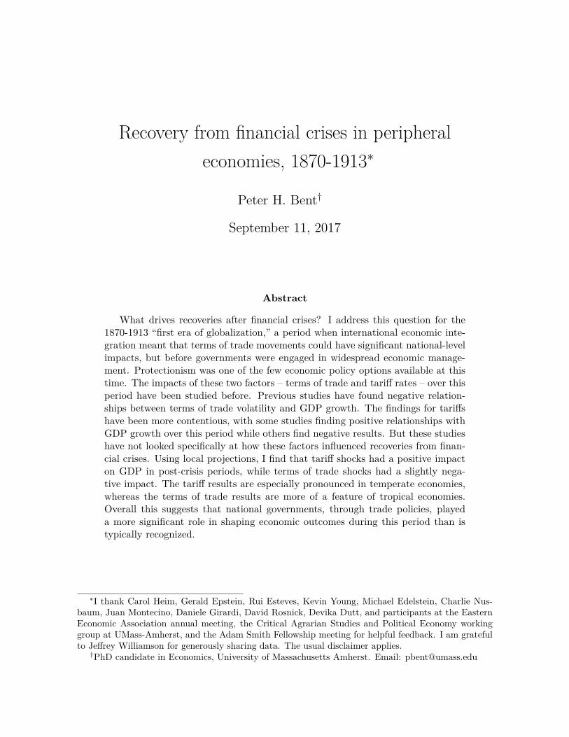
What drives recoveries after financial crises? I address this question for the1870-1913 “first era of globalization,” a period when international economic inte-gration meant that terms of trade movements could have significant national-levelimpacts, but before governments were engaged in widespread economic manage-ment. Protectionism was one of the few economic policy options available at thistime. The impacts of these two factors – terms of trade and tariff rates – over thisperiod have been studied before. Previous studies have found negative relation-ships between terms of trade volatility and GDP growth. The findings for tariffshave been more contentious, with some studies finding positive relationships withGDP growth over this period while others find negative results. But these studieshave not looked specifically at how these factors influenced recoveries from finan-cial crises. Using local projections, I find that tariff shocks had a positive impacton GDP in post-crisis periods, while terms of trade shocks had a slightly nega-tive impact. The tariff results are especially pronounced in temperate economies,whereas the terms of trade results are more of a feature of tropical economies.Overall this suggests that national governments, through trade policies, playeda more significant role in shaping economic outcomes during this period than istypically recognized.

∗I thank Carol Heim, Gerald Epstein, Rui Esteves, Kevin Young, Michael Edelstein, Charlie Nus-baum, Juan Montecino, Daniele Girardi, David Rosnick, Devika Dutt, and participants at the EasternEconomic Association annual meeting, the Critical Agrarian Studies and Political Economy workinggroup at UMass-Amherst, and the Adam Smith Fellowship meeting for helpful feedback. I am gratefulto Jeffrey Williamson for generously sharing data. The usual disclaimer applies.†PhD candidate in Economics, University of Massachusetts Amherst. Email: pbent@umass.edu

“To excuse an indifference towards the control of depressions because the latter are alwaysfollowed by revival is, indeed, tantamount to saying that we should not seek to abolish orlessen wars because they, too, are always followed by a period of peace.” Paul Douglas(U.S. Senator and economist) (1935, pp. 80-81)

1 Introduction

The 2007-08 financial crisis generated renewed interest in the factors that cause financialcrises. But as more time has passed, attention has turned toward recoveries from crises.Since developed countries did not experience many crises over the second half of thetwentieth century, this line of research has had to reach further back into history totimes of greater macroeconomic turbulence to investigate a larger sample of recoveryperiods.

Reinhart and Rogoff (2014), for example, present a comprehensive overview of theavailable historical data on recoveries from financial crises. They measure the number ofyears for business cycle peaks-to-troughs and peaks-to-recoveries over 100 crisis periodsfrom 1857-2013.1 Other long-run and historical studies of recoveries from financial crisestend to be more narrowly focused on specific periods, especially the Great Depression.2

In this paper I focus on the 1870-1913 period, which saw an especially large number ofcrises. Several previous studies are particularly relevant for the task at hand. Empiri-cally, I follow Rocha and Solomou (2015) and Romer and Romer (2016) by using Jordà’s(2005) local projection method to analyze post-crisis recovery periods. Specifically, I testthe impact that terms of trade3 and tariff4 shocks have on economic output in post-crisisperiods.

Improving terms of trade have been connected with higher GDP levels and growth1Related studies of the recoveries from financial crises include Baldacci, Gupta, and Mulas-Granados

(2009), Fatás and Mihov (2013), Ha and Kang (2015), Reinhart and Rogoff (2009a, 2009b). Also seethe research on whether recoveries occur as “Phoenix Miracles” (when recoveries happen without areliance on credit): Calvo, Izquierdo, and Talvi (2006), Biggs, Mayer, and Pick (2010). Additionally,Brunnermeier and Schabel (2016) study 400 years of bubbles, crises, and recoveries, looking at centralbanks’ roles through each of these business cycle phases.

2Economic studies of the interwar period are too numerous to cite here in full, but several recentstudies that focus on recovery during the 1930s include Eggertsson (2012), Payne and Uren (2014), Jaliland Rua (2016), Taylor and Neumann (2016), Chouliarakis and Gwiazdowski (2017), and Hausman,Rhode, and Wieland (2017). A contemporary study focusing on the question of recovery at this timeis Brown et al. (1968 [1934]).

3Terms of trade is the ratio of export to import prices. See Section 4 for details.4Tariff rates are measured as total government revenue from imports over the value of imports to a

given country in a given year. See Section 4 for details.

1

rates.5 This could occur through a capital accumulation channel (Blattman, Hwang,and Williamson, 2007), or through productivity improvements due to the ability toimport more productivity-enhancing capital goods (Basu and McLeod, 1992). In thelong run, however, investment could be tempered by a “resource curse” effect (Sachsand Warner, 1995, 2001), or rent-seeking behavior among resource rich elites (Krueger,1974). Blattman et al. (2007) contribute to this research by distinguishing between termsof trade growth and volatility.6 They find a significant negative relationship betweenterms of trade volatility and economic growth in peripheral countries from 1870-1939,versus no significant relationship between terms of trade growth and income growth.Their approach is based on medium to long-run time frames (2007, p. 168). Researchlooking at the relationship between terms of trade movements and economic growth inrecent decades also takes a longer-run approach (Easterly, Kremer, Pritchett, Summers,1993; Rodrik, 1999; Berg, Ostry, and Zettelmeyer, 2012). In contrast, I focus on themore immediate effects that terms of trade movements can have on output, particularlyduring the several years after financial crises.7

The 1870-1913 period is known as the “first era of globalization” for its high lev-els of international capital, labor, and trade movements. This period is also notablefor the numerous and severe financial crises that occurred. While the interwar periodbrought increased government involvement in directing economic activity, the pre-WorldWar I period was much more laissez-faire. Overt management of economies by nationalgovernments was negligible, with tariff policies being one of the few government inter-ventions in peripheral economies.8 To address the question of which factors played amore significant role in helping economies recover from crises, terms of trade measuresand tariff rates are the best available data we have for comparing whether changes inmarket conditions (commodity prices accounted for by terms of trade measures) or gov-ernment actions (specifically tariff policies) had more of an impact on GDP growth inthe wake of financial crises.

One of the few measurable factors that affected the severity of economic downturns5Blattman et al. (2007, p. 160) present a useful overview of this literature.6Blattman et al. (2007, p. 166) use the Hodrick-Prescott (HP) filter to calculate these two factors,

terms of trade growth (a smooth trend) and volatility (stationary deviations).7Some other studies, such as Funke, Granziera, and Imam (2008), use annual data in their analysis

of how terms of trade shocks impacted economic growth from 1970-2006, but as far as I know this isthe first paper to use annual data to specifically focus on post-crisis periods for the 1870-1913 period.

8This “laissez-faire” narrative is challenged by recent research looking at the scale of both nationaland local government involvement in shaping economic outcomes during this period (Novak, 1996, 2008;Palen, 2015).

2

at this time was a country’s terms of trade. This was noted in early studies of thisperiod. Argentina’s recovery after the 1890 Baring Crisis, for example, was prolongedin part because of depressed commodity prices (Ford, 1956), and recovery in the UnitedStates after the 1893 panic was boosted when commodity prices increased in 1897 (aftera double-dip recession occurred in 1896) (White, 1939). Terms of trade data allow theserelationships between commodity price movements and broader economic recovery aftercrises to be tested across peripheral economies over this period.

Tariff policy was one of the main avenues through which national governments couldimpact economic outcomes at this time. In the United States, for example, one of themain protectionist arguments in the 1890s was that higher tariff rates would promoterecovery from the 1893 panic and subsequent depression by assuring producers of bothagricultural and manufactured goods that they would benefit under a newly protectionistregime (Bent 2015a, 2015b). There is an extensive literature on tariff rates and economicgrowth more broadly for this period, with the general finding that higher tariffs wereassociated with higher economic growth rates, at least before the mid-twentieth cen-tury (O’Rourke, 2000; Clemens and Williamson, 2004b; Lehmann and O’Rourke, 2011;Lampe and Sharpe, 2013), though the direction of causation is not always clear (Irwin,2002a, 2002b). This paper contributes to this literature by focusing on the relationshipbetween tariffs and growth specifically during post-crisis periods, to test protectionists’claims that higher tariff rates would stabilize expectations and promote investment andgrowth after crises.

The cross-country analysis in this paper tests for the impact that terms of changemovements and tariff rates had on economic growth during the globally interconnectedand macroeconomically volatile 1870-1913 period. The main empirical finding is thattariff rate shocks had a significant positive impact on GDP growth in post-crisis periods,whereas terms of trade shocks had a slightly negative impact. The tariff results areespecially pronounced in temperate economies, whereas the terms of trade results aremore of a feature of tropical economies. Altogether this adds to our understandingof how economies recover from financial crises. I conclude that recoveries, especiallyin the more developed peripheral economies, were due more to government action (atleast partly intended to improve macroeconomic performance) than to exogenous marketforces.

3

2 Terms of trade and economic growth

The countries included in this study had largely agricultural economies, which tendedto be dominated by a few commodities whose price movements could have broadermacroeconomic effects. Describing these trends for the United States at the turn of thetwentieth century, the economist A. Piatt Andrew made the following remarks:

An unusually large harvest in this country, if accompanied by small har-vests abroad, obviously means prosperity for the American farmers, meanslarge exports and high prices, tends to mean incoming gold and expand-ing credit. But, if accompanied by excessive crops abroad and flagging de-mand, it means, on the other hand, extraordinarily low prices, diminishedexports, and depression in agriculture, if not in general trade (1906, p. 329).. . . [T]he beginnings of every movement toward business prosperity and theturning-points toward every business decline . . . were closely connected withthe out-turn of crops (ibid., p. 351).

What was true for the United States and other developing economies a hundredyears ago remains relevant for developing countries today. The long-run connectionsbetween commodity price fluctuations and sovereign defaults are illustrated in Reinhart,Reinhart, and Trebesch (2016), with data on boom-bust cycles over the past 200 years.These relationships were relevant during the 2007-08 crisis (Shelburne, 2010; Bloch andSapsford, 2011) just as they were for crises at the turn of the last century (Andrew,1906; Davis, Hanes, and Rhode, 2009).

Terms of trade movements have been associated with changes in economic outputand growth more generally. Basu and McLeod (1992), for example, find long-run effectson output for even short-term export price shocks. Similarly, terms of trade shocks helpexplain differences in growth trajectories across countries, beyond what can be deter-mined by country characteristics such as education levels (Easterly, Kremer, Pritchett,and Summers, 1993).9 That such shocks have different effects in different countries hasalso been documented in specific African cases by Deaton (1999), Imam and Salinas(2008), and Fosu (2011).

9Hadass and Williamson (2003, p. 651) suggest otherwise, in their long-run empirical analysis ofthe Prebisch-Singer hypothesis: “It appears that the great terms-of-trade debate was about an eventthat was pretty minor for most participants in the center and the periphery. The fundamentals insidethese countries mattered most to growth, just as they do today.” While that accounts for the long-run relationship between terms of trade and economic growth, the analysis in this paper focuses morenarrowly on terms of trade changes in the aftermath of financial crises.

4

Methodologically, it has been found that analyzing the impact of terms of tradegrowth and volatility separately makes a difference for explaining the impact of termsof trade movements on economic growth. Blattman, Hwang, and Williamson (2007), forexample, find a negative relationship between terms of trade volatility and output from1870-1939, but no significant relationship between terms of trade growth and economicoutput. Turnovsky and Chattopadhyay (2003) find similar results for the last quarterof the twentieth century. Relatedly, Basu and McLeod (1992) find that export pricevolatility decreases domestic investment. More narrowly, Bidarkota and Crucini (2000)highlight the importance of accounting for particular commodities when studying termsof trade volatility in developing countries.

Of the different types of shocks developing countries can experience, Becker andMauro (2006) find negative terms of trade shocks to have the most severe impact on eco-nomic output. Rodrik (1999) and Jerzmanowski (2006) argue that institutions explainmuch of a country’s ability to recover from such shocks.10 Similarly, Funke, Granziera,and Imam (2008) study the role that particular institutional variables play in recoveryperiods from 1970-2006. The same range of variables is not available for the 1870-1913period, but they would be less relevant, since national governments in general did nottake as active a role in shaping their country’s economies, and estimates of institu-tional quality would be less informative. My approach is to assess the overall impactthat terms of trade shocks had on economies in post-crisis periods in order to see whatfactors contributed to, or hindered, recoveries from financial crises at this time.

3 Tariffs and economic growth

While national governments in developing countries mostly took a hands-off approachto their economies over the late nineteenth and early twentieth centuries, tariff policieswere one of the few ways they directly impacted economic activity. Tariffs can spureconomic growth by supporting development through infant industry protection (List,1909[1841]; Amsden, 1989).11 In the late nineteenth century, tariffs were also a mainsource of government revenue, and balancing the budget was a stated aim of protection-

10Rodrik (1999) uses indicators of the quality of governmental institutions, rule of law, democraticrights, and social safety nets as proxies for institutions of conflict management. Jerzmanowski (2006, p.366) measures institutional quality with an index based on measures of rule of law, risk of expropriation,corruption, bureaucratic quality, and government repudiation contracts.

11Allen (2011) presents a useful overview of different countries’ experiences with protectionismthrough the nineteenth and twentieth centuries.

5

ists.12 Additionally, the case of the United States during the 1890s depression suggeststhat decisive increases in tariff rates in the wake of financial crises can signal that thegovernment is willing to protect the domestic economy from foreign competition.13

Rodríguez and Rodrik (2000, pp. 267-68) summarize contemporary theories aboutthe impact trade restrictions have on real GDP. Accounting for static models with nomarket imperfections, neoclassical growth models, and endogenous growth models, theynote that “there should be no theoretical presumption in favor of finding an unam-biguous, negative relationship between trade barriers and growth rates in the types ofcross-national data sets typically analyzed” (ibid., p. 268). These theories also allowfor short and long term positive connections between protectionist policies and GDPgrowth, such as when import-competing sectors have positive production externalities,or when technologically dynamic industries are promoted more strongly in endogenousgrowth models (ibid).

Empirical studies spanning the 1870-1913 period have analyzed the connections be-tween average measures of protection and economic growth (O’Rourke, 2000; Vam-vakidis, 2002; Clemens and Williamson, 2004b; Schularick and Solomou, 2011, Jacks,2013). A more extensive literature addresses this issue for recent decades.14 Whileearly studies (O’Rourke, 2000; Clemens and Williamson, 2004b) found that the over-all relationship between tariffs and growth was positive for the late nineteenth century,increasingly the evidence suggests that this relationship is “complex, time-varying andmay display significant heterogeneity” (Schularick and Solomou, 2011, p. 35). Lehmannand O’Rourke (2011) build on this research by exploring the connections between vari-ous types of tariffs – agricultural, industrial, or revenue (luxury goods) – based on thepremise that different countries imported different commodities, and that average tariffrates hide important differences across sectors.

These studies use panel data to analyze broad trends across countries. In contrast,Lampe and Sharp (2013) use time series methods to explore the connections betweenchanges in tariff rates and economic growth on a country-by-country basis, addressingthe importance of cross-country heterogeneity as highlighted by Schularick and Solomou(2011). In contrast to earlier panel data studies, Lampe and Sharp (2013) find that while

12E.g., for Republicans in the United States.13Disentangling the stated goal of promoting national prosperity from unstated goals of aiding specific

interest groups through tariff policies is difficult (Stern, 1971, p. viii; Bent, 2015a).14There are many overviews of this literature available. Rodríguez and Rodrik (2000) is a useful, if

slightly dated, starting point. Schularick and Solomou (2011) present a more recent discussion of thisliterature, covering both historical and more recent periods.

6

the relationship between tariffs and income differed by country, for most countries theoverall relationship between tariffs and income was negative. Other research has focusedon individual countries, such as a recent study of turn of the century Switzerland. Forthe Swiss case, Charles (2017) finds that “moderate and selective” protectionism from1886-1913 “Granger-causes” increased exports from new industries.

Supporting the use of such case studies is Irwin’s (2002b) argument that cross-countryanalyses of tariffs and growth have significant limitations. Irwin argues that for cross-country studies focused on this period, results showing positive correlation between hightariffs and high growth can be driven by countries such as Argentina and Canada, whichhad economies based on export crops rather than import-substitution industrialization.Irwin concludes that “[r]ather than higher tariffs causing higher growth, the relationshipcould be spurious: land-abundant countries relied on customs duties to raise governmentrevenue and also enjoyed favorable growth prospects, with little link between the two”(Irwin, 2002b, p. 169). This is a useful critique of the existing literature, and one that Iaddress in another paper, employing detailed case studies to complement cross-countryempirical analyses. Also, it is important to note that by focusing here on post-crisisperiods, I do not address long-run trends, but rather look more narrowly at the short-run impact of tariff shocks in the context of post-crisis economic downturns.

The goal of this paper is not to make new claims about the overall connectionsbetween trade openness and economic growth across this whole period, whether mostlypositive, negative, or heterogeneous in different countries. Instead I address the observa-tion that this relationship could be time-varying (Schularick and Solomou, 2011), which,I argue, is especially important to recognize with regard to how tariff policy impactedeconomies in the aftermath of financial crises.

A final question about tariffs is whether tariff rate changes can be accurately de-scribed as exogenous shocks. Terms of trade shocks, for example, can occur when a nat-ural disaster significantly impacts the price of an export commodity. In contrast, tariffchanges are more likely to be anticipated, as they are determined politically (Williamson,2006, p. 199). Still, the empirical literature on trade restrictions accounts for tar-iff “shocks” as well as gradual changes in tariff rates (Auernheimer and George, 1997;Malakellis, 1998). Sometimes governments deliberately phase in tariffs gradually in or-der to reduce the shock effect (Irwin, 2014, p. 8). While some tariff policy changes areanticipated and/or gradual, treating tariffs changes as shocks is common practice in theempirical trade literature (Lanclos and Hertel, 1995; Spearot, 2016).

7

4 Data and framework

The main variables used in this study are terms of trade, tariff rates, and GDP estimatescovering 35 countries for the years 1870-1913. The terms of trade data come fromBlattman, Hwang, and Williamson’s (2007) database15 and the tariff rate data are fromClemens and Williamson (2004b). Terms of trade is the ratio of export to import prices,and tariff rates are calculated as total government revenue from imports over the valueof imports to that country in that year. The GDP series from the Blattman et al.database are mostly from Maddison (1995) but are supplemented with other data serieswhen available.

The other main variables of interest are financial crisis indicators. For this timeperiod, the available measures of financial crises are binary variables, equaling one if acrisis occurred in a particular country in a given year, and zero otherwise. There are datafor banking crises (Reinhart and Rogoff, 2009b), currency crises (Bordo and Meissner,2011), and sovereign defaults (Suter, 1990) (see table A.1 in the data appendix).16 Forthe sovereign default data, I focus on the first year of default periods in order to isolatethe onset of an actual crisis rather than accounting for prolonged default episodes. Inorder to have a sufficiently large sample of recovery periods, I focus on recoveries fromeach of these crisis types together. That is, I code the crisis data as an encompassingmeasure of whether any type of crisis – banking, currency, or default – occurred in acountry-year observation, and then test how terms of trade and tariff shocks impactedGDP in those post-crisis periods.17

Previous studies of the relationship between terms of trade measures and economicgrowth use five- or ten-year averages in order to account for long-run trends (Hadassand Williamson, 2003; Blattman, Hwang, and Williamson, 2007). The same is true forstudies of connections between tariff rates and GDP growth over this period (Lehmannand O’Rourke, 2011; O’Rourke, 2000; Lampe and Sharpe, 2013). In contrast, I aminterested in the short-run impact of terms of trade and tariff shocks specifically in post-crisis contexts. I thus use annual data. There are shortcomings to this approach, dueto the imprecision of the data. The export and import data that are used to constructthe terms of trade ratio are difficult to find for all countries and years in this sample.

15The terms of trade data are constructed by Blattman et al. (2007, p. 163) from commodity priceseries. I am grateful to Jeffrey Williamson for sharing an updated version of this database with me(September 2016).

16The currency crisis data begin in 1880. An updated version of Suter’s book was published in Englishin 1992.

17In the robustness section I focus on specific types of crises separately.

8

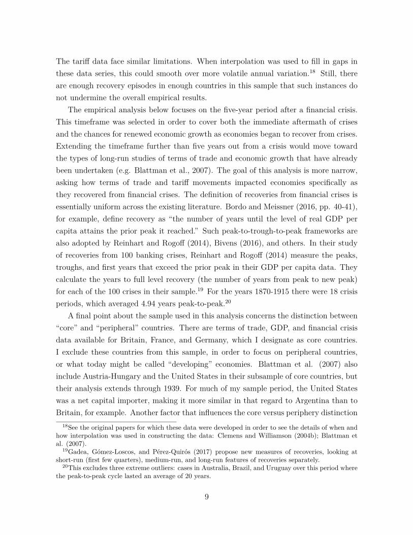
The tariff data face similar limitations. When interpolation was used to fill in gaps inthese data series, this could smooth over more volatile annual variation.18 Still, thereare enough recovery episodes in enough countries in this sample that such instances donot undermine the overall empirical results.

The empirical analysis below focuses on the five-year period after a financial crisis.This timeframe was selected in order to cover both the immediate aftermath of crisesand the chances for renewed economic growth as economies began to recover from crises.Extending the timeframe further than five years out from a crisis would move towardthe types of long-run studies of terms of trade and economic growth that have alreadybeen undertaken (e.g. Blattman et al., 2007). The goal of this analysis is more narrow,asking how terms of trade and tariff movements impacted economies specifically asthey recovered from financial crises. The definition of recoveries from financial crises isessentially uniform across the existing literature. Bordo and Meissner (2016, pp. 40-41),for example, define recovery as “the number of years until the level of real GDP percapita attains the prior peak it reached.” Such peak-to-trough-to-peak frameworks arealso adopted by Reinhart and Rogoff (2014), Bivens (2016), and others. In their studyof recoveries from 100 banking crises, Reinhart and Rogoff (2014) measure the peaks,troughs, and first years that exceed the prior peak in their GDP per capita data. Theycalculate the years to full level recovery (the number of years from peak to new peak)for each of the 100 crises in their sample.19 For the years 1870-1915 there were 18 crisisperiods, which averaged 4.94 years peak-to-peak.20

A final point about the sample used in this analysis concerns the distinction between“core” and “peripheral” countries. There are terms of trade, GDP, and financial crisisdata available for Britain, France, and Germany, which I designate as core countries.I exclude these countries from this sample, in order to focus on peripheral countries,or what today might be called “developing” economies. Blattman et al. (2007) alsoinclude Austria-Hungary and the United States in their subsample of core countries, buttheir analysis extends through 1939. For much of my sample period, the United Stateswas a net capital importer, making it more similar in that regard to Argentina than toBritain, for example. Another factor that influences the core versus periphery distinction

18See the original papers for which these data were developed in order to see the details of when andhow interpolation was used in constructing the data: Clemens and Williamson (2004b); Blattman etal. (2007).

19Gadea, Gómez-Loscos, and Pérez-Quirós (2017) propose new measures of recoveries, looking atshort-run (first few quarters), medium-run, and long-run features of recoveries separately.

20This excludes three extreme outliers: cases in Australia, Brazil, and Uruguay over this period wherethe peak-to-peak cycle lasted an average of 20 years.

9

for Blattman et al. (2007) is whether an economy was large enough to influence globalprices for a particular commodity, and whether a country exported manufactures. TheUnited States poses a problem on both these counts, so it is excluded from some of theeconometric tests below to check that it is not unduly influencing the main results.

5 Empirical analysis

5.1 General trends

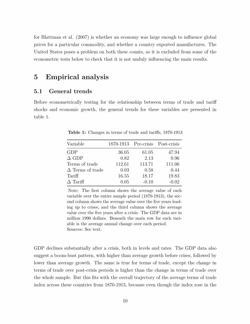
Before econometrically testing for the relationship between terms of trade and tariffshocks and economic growth, the general trends for these variables are presented intable 1.

Table 1: Changes in terms of trade and tariffs, 1870-1913

Variable 1870-1913 Pre-crisis Post-crisisGDP 36.05 61.05 47.94∆ GDP 0.82 2.13 0.96Terms of trade 112.61 113.71 111.06∆ Terms of trade 0.03 0.58 0.44Tariff 16.55 18.17 19.83∆ Tariff 0.05 -0.10 -0.02Note: The first column shows the average value of eachvariable over the entire sample period (1870-1913), the sec-ond column shows the average value over the five years lead-ing up to crises, and the third column shows the averagevalue over the five years after a crisis. The GDP data are inmillion 1990 dollars. Beneath the main row for each vari-able is the average annual change over each period.Sources: See text.

GDP declines substantially after a crisis, both in levels and rates. The GDP data alsosuggest a boom-bust pattern, with higher than average growth before crises, followed bylower than average growth. The same is true for terms of trade, except the change interms of trade over post-crisis periods is higher than the change in terms of trade overthe whole sample. But this fits with the overall trajectory of the average terms of tradeindex across these countries from 1870-1913, because even though the index rose in the

10

1880s and fell in the 1890s, these peaks and troughs average out to little change overthe whole period. In contrast, tariff rates were on average higher in post-crisis periodscompared to pre-crisis periods and the sample average.

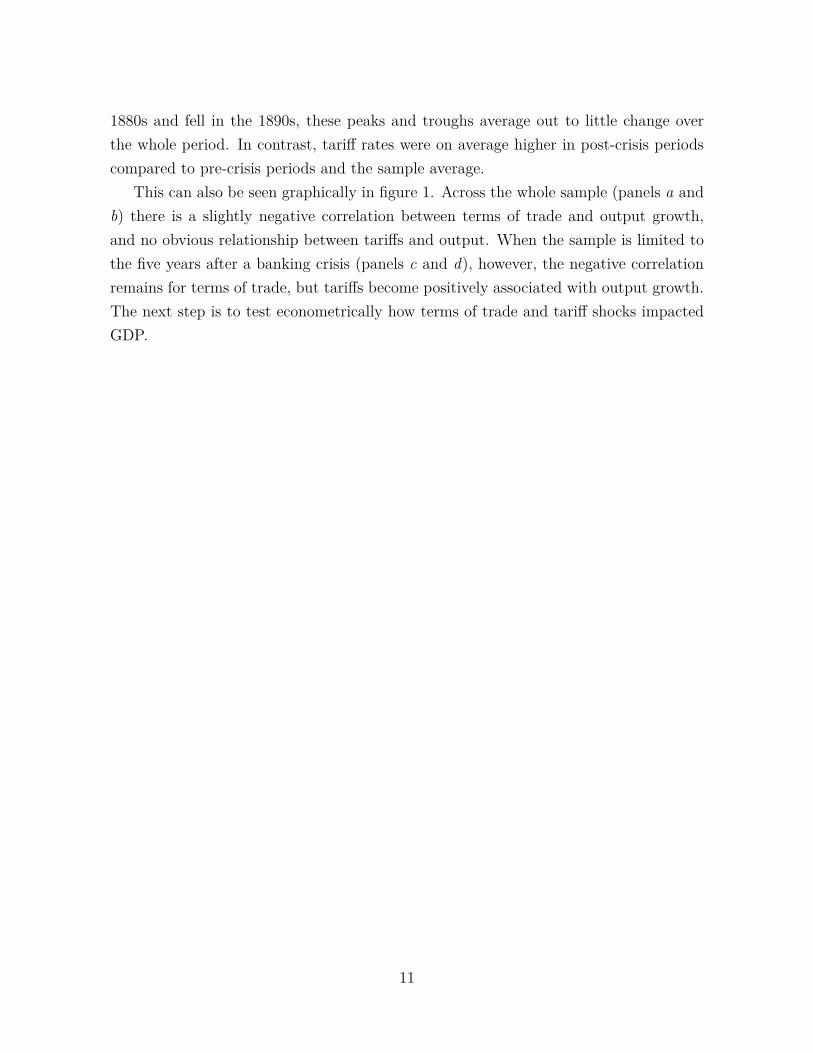
This can also be seen graphically in figure 1. Across the whole sample (panels a andb) there is a slightly negative correlation between terms of trade and output growth,and no obvious relationship between tariffs and output. When the sample is limited tothe five years after a banking crisis (panels c and d), however, the negative correlationremains for terms of trade, but tariffs become positively associated with output growth.The next step is to test econometrically how terms of trade and tariff shocks impactedGDP.

11

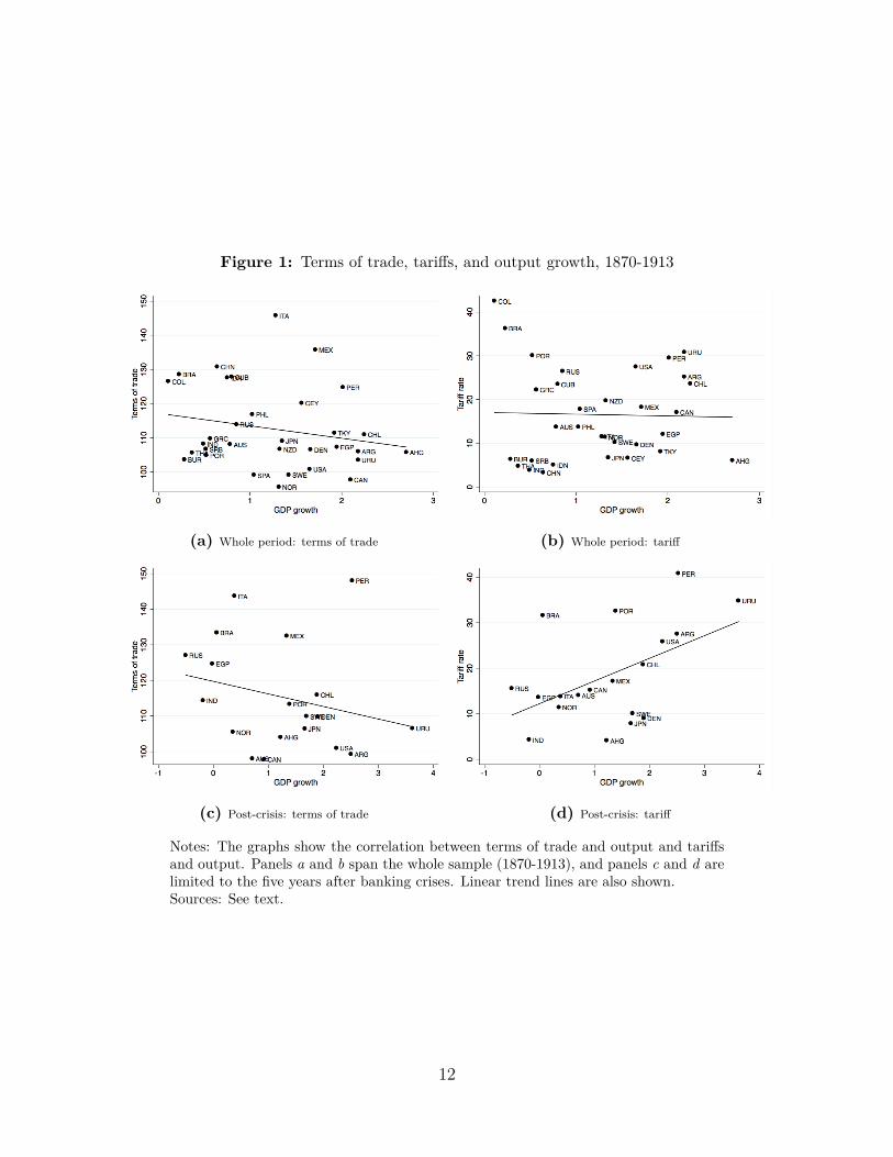
Figure 1: Terms of trade, tariffs, and output growth, 1870-1913

(a) Whole period: terms of trade (b) Whole period: tariff

(c) Post-crisis: terms of trade (d) Post-crisis: tariff

Notes: The graphs show the correlation between terms of trade and output and tariffsand output. Panels a and b span the whole sample (1870-1913), and panels c and d arelimited to the five years after banking crises. Linear trend lines are also shown.Sources: See text.

12

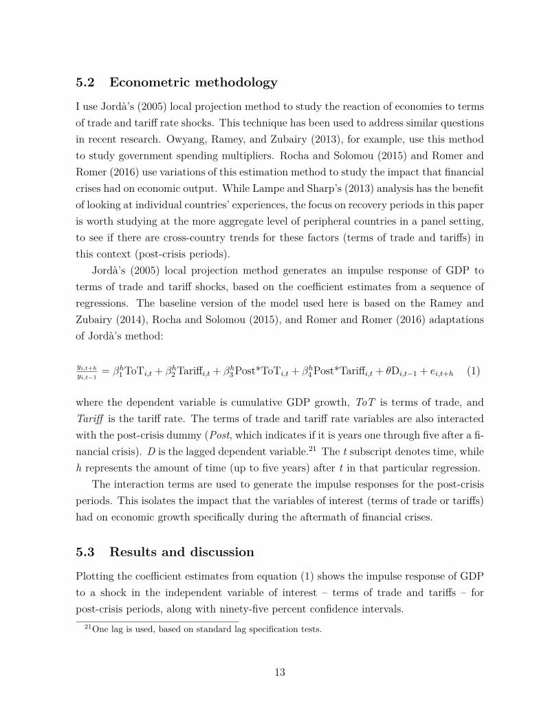
5.2 Econometric methodology

I use Jordà’s (2005) local projection method to study the reaction of economies to termsof trade and tariff rate shocks. This technique has been used to address similar questionsin recent research. Owyang, Ramey, and Zubairy (2013), for example, use this methodto study government spending multipliers. Rocha and Solomou (2015) and Romer andRomer (2016) use variations of this estimation method to study the impact that financialcrises had on economic output. While Lampe and Sharp’s (2013) analysis has the benefitof looking at individual countries’ experiences, the focus on recovery periods in this paperis worth studying at the more aggregate level of peripheral countries in a panel setting,to see if there are cross-country trends for these factors (terms of trade and tariffs) inthis context (post-crisis periods).

Jordà’s (2005) local projection method generates an impulse response of GDP toterms of trade and tariff shocks, based on the coefficient estimates from a sequence ofregressions. The baseline version of the model used here is based on the Ramey andZubairy (2014), Rocha and Solomou (2015), and Romer and Romer (2016) adaptationsof Jordà’s method:

yi,t+h

yi,t−1= βh

1ToTi,t + βh2Tariffi,t + βh

3Post*ToTi,t + βh4Post*Tariffi,t + θDi,t−1 + ei,t+h (1)

where the dependent variable is cumulative GDP growth, ToT is terms of trade, andTariff is the tariff rate. The terms of trade and tariff rate variables are also interactedwith the post-crisis dummy (Post, which indicates if it is years one through five after a fi-nancial crisis). D is the lagged dependent variable.21 The t subscript denotes time, whileh represents the amount of time (up to five years) after t in that particular regression.

The interaction terms are used to generate the impulse responses for the post-crisisperiods. This isolates the impact that the variables of interest (terms of trade or tariffs)had on economic growth specifically during the aftermath of financial crises.

5.3 Results and discussion

Plotting the coefficient estimates from equation (1) shows the impulse response of GDPto a shock in the independent variable of interest – terms of trade and tariffs – forpost-crisis periods, along with ninety-five percent confidence intervals.

21One lag is used, based on standard lag specification tests.

13

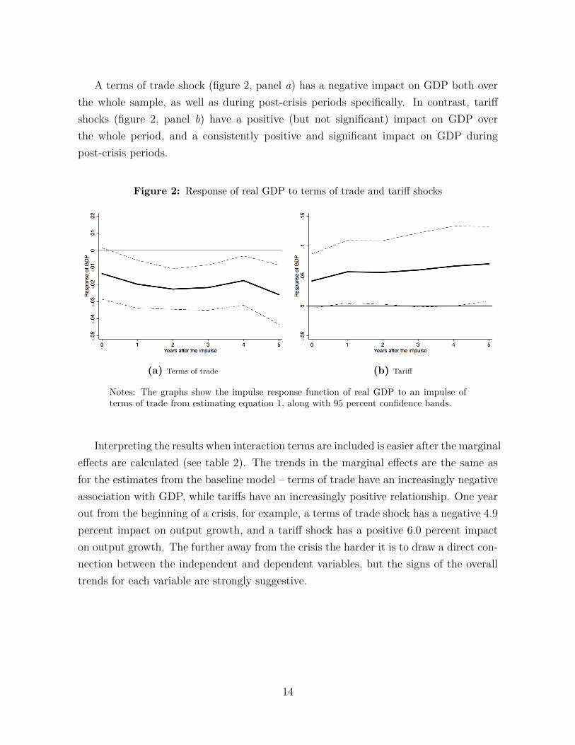
A terms of trade shock (figure 2, panel a) has a negative impact on GDP both overthe whole sample, as well as during post-crisis periods specifically. In contrast, tariffshocks (figure 2, panel b) have a positive (but not significant) impact on GDP overthe whole period, and a consistently positive and significant impact on GDP duringpost-crisis periods.

Figure 2: Response of real GDP to terms of trade and tariff shocks

(a) Terms of trade (b) Tariff

Notes: The graphs show the impulse response function of real GDP to an impulse ofterms of trade from estimating equation 1, along with 95 percent confidence bands.

Interpreting the results when interaction terms are included is easier after the marginaleffects are calculated (see table 2). The trends in the marginal effects are the same asfor the estimates from the baseline model – terms of trade have an increasingly negativeassociation with GDP, while tariffs have an increasingly positive relationship. One yearout from the beginning of a crisis, for example, a terms of trade shock has a negative 4.9percent impact on output growth, and a tariff shock has a positive 6.0 percent impacton output growth. The further away from the crisis the harder it is to draw a direct con-nection between the independent and dependent variables, but the signs of the overalltrends for each variable are strongly suggestive.

14

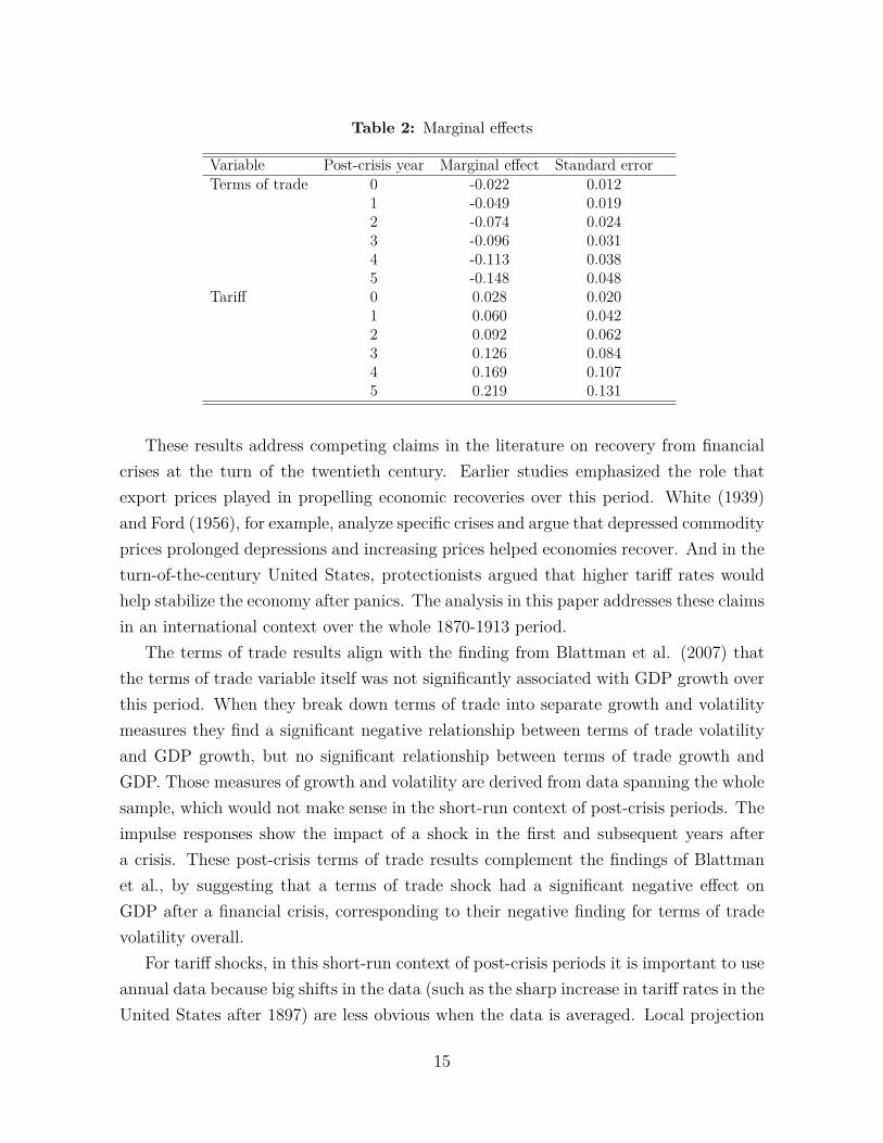
Table 2: Marginal effects

Variable Post-crisis year Marginal effect Standard errorTerms of trade 0 -0.022 0.012

1 -0.049 0.0192 -0.074 0.0243 -0.096 0.0314 -0.113 0.0385 -0.148 0.048

Tariff 0 0.028 0.0201 0.060 0.0422 0.092 0.0623 0.126 0.0844 0.169 0.1075 0.219 0.131

These results address competing claims in the literature on recovery from financialcrises at the turn of the twentieth century. Earlier studies emphasized the role thatexport prices played in propelling economic recoveries over this period. White (1939)and Ford (1956), for example, analyze specific crises and argue that depressed commodityprices prolonged depressions and increasing prices helped economies recover. And in theturn-of-the-century United States, protectionists argued that higher tariff rates wouldhelp stabilize the economy after panics. The analysis in this paper addresses these claimsin an international context over the whole 1870-1913 period.

The terms of trade results align with the finding from Blattman et al. (2007) thatthe terms of trade variable itself was not significantly associated with GDP growth overthis period. When they break down terms of trade into separate growth and volatilitymeasures they find a significant negative relationship between terms of trade volatilityand GDP growth, but no significant relationship between terms of trade growth andGDP. Those measures of growth and volatility are derived from data spanning the wholesample, which would not make sense in the short-run context of post-crisis periods. Theimpulse responses show the impact of a shock in the first and subsequent years aftera crisis. These post-crisis terms of trade results complement the findings of Blattmanet al., by suggesting that a terms of trade shock had a significant negative effect onGDP after a financial crisis, corresponding to their negative finding for terms of tradevolatility overall.

For tariff shocks, in this short-run context of post-crisis periods it is important to useannual data because big shifts in the data (such as the sharp increase in tariff rates in theUnited States after 1897) are less obvious when the data is averaged. Local projection

15

results for the whole sample22 show that tariff shocks did not have significant impactson GDP growth. However, when the sample is limited to the aftermath of financialcrises (figure 2, panel b), higher tariff rates positively impact GDP. This highlights theimportance of not simply taking consecutive five-year averages of the data, but ratherfocusing on the context in which tariff rate changes occurred (e.g., whether or not therewas a financial crisis). This does not necessarily call into the question the results othershave found for this period, but it does highlight the particularly strong impact that tariffpolicies could have in the wake of financial crises.

These findings also align with theories that suggest the short-term impact of tariffswould be positive (by protecting domestic industry and encouraging investment) butthat the long-run impact would be negative (as firms grew complacent and inefficient asa result of being protected from competition, for example, and/or through deadweightlosses).23 Additionally, there are particular short-run concerns that are heightened in theaftermath of crises, namely the desire to promote stability and manage expectations byassuring firms and investors that the government has a plan for what trade policies willbe implemented. As the mayor of New York City complained in 1897, it is “constant andrepeated changes [in tariff rates] that unsettle the business of this country” (“DingleyBill Discussed”). Tariff policies were one of the few options available for governments inthese developing countries to intervene in their economies at this time, and this evidencesuggests that such policies were associated with renewed output growth after financialcrises.

5.4 Robustness

One potential issue with this empirical strategy is that the results found for the post-crisisperiods could simply be a consequence of looking at five-year periods rather than all theyears in the sample. To be assured that this is not the case, I run the main regressionsagain but replace the post-crisis indicator in equation 1 with a dummy variable for thefive years preceding a crisis. The results are for the pre-crisis period are very different,with the tariff interaction results negative and insignificant. This suggests that therelationships between terms of trade and output growth and between tariffs and outputgrowth were different during the pre- versus post-crisis periods, with tariffs having anespecially strong impact on crises in the post-crisis periods.

22These graphs are omitted here but are available upon request.23See Bastiat (2007 [1850], pp. 24-29) for a useful historical illustration of the longer-run negative

effects of tariffs.

16

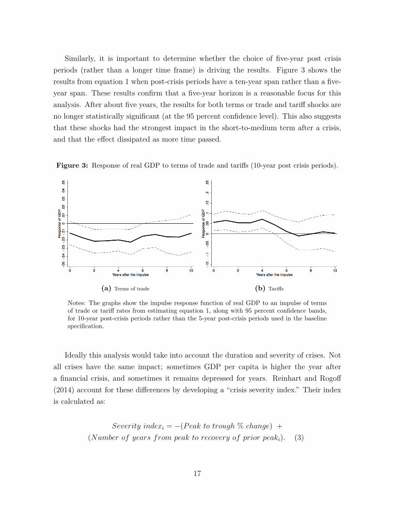
Similarly, it is important to determine whether the choice of five-year post crisisperiods (rather than a longer time frame) is driving the results. Figure 3 shows theresults from equation 1 when post-crisis periods have a ten-year span rather than a five-year span. These results confirm that a five-year horizon is a reasonable focus for thisanalysis. After about five years, the results for both terms or trade and tariff shocks areno longer statistically significant (at the 95 percent confidence level). This also suggeststhat these shocks had the strongest impact in the short-to-medium term after a crisis,and that the effect dissipated as more time passed.

Figure 3: Response of real GDP to terms of trade and tariffs (10-year post crisis periods).

(a) Terms of trade (b) Tariffs

Notes: The graphs show the impulse response function of real GDP to an impulse of termsof trade or tariff rates from estimating equation 1, along with 95 percent confidence bands,for 10-year post-crisis periods rather than the 5-year post-crisis periods used in the baselinespecification.

Ideally this analysis would take into account the duration and severity of crises. Notall crises have the same impact; sometimes GDP per capita is higher the year aftera financial crisis, and sometimes it remains depressed for years. Reinhart and Rogoff(2014) account for these differences by developing a “crisis severity index.” Their indexis calculated as:

Severity indexi = −(Peak to trough % change) +(Number of years from peak to recovery of prior peaki). (3)

17

That index accounts for 100 crisis episodes, each denoted by the i subscript in equation3, over more than 150 years and a wide range of countries. Combined with peak-to-trough and peak-to-recovery timelines and an indicator of whether or not there was adouble-dip, the index offers a way to compare recovery periods across different countriesand times. Incorporating such an index into the analysis in this paper would be usefulbecause, for example, it would provide information about whether terms of trade or tariffshocks coincided with mild or severe crises. Unfortunately, the sample in this paper istoo limited to undertake that kind of analysis. There are 37 banking banking crises inmy sample, and in only 12 of those cases did post-crisis GDP per capita decrease for oneor more years. In future research, extended series of terms of trade and tariff rate datacould be combined with Reinhart and Rogoff’s (2014) crisis severity index to conduct alonger-run study of interactions between those variables.

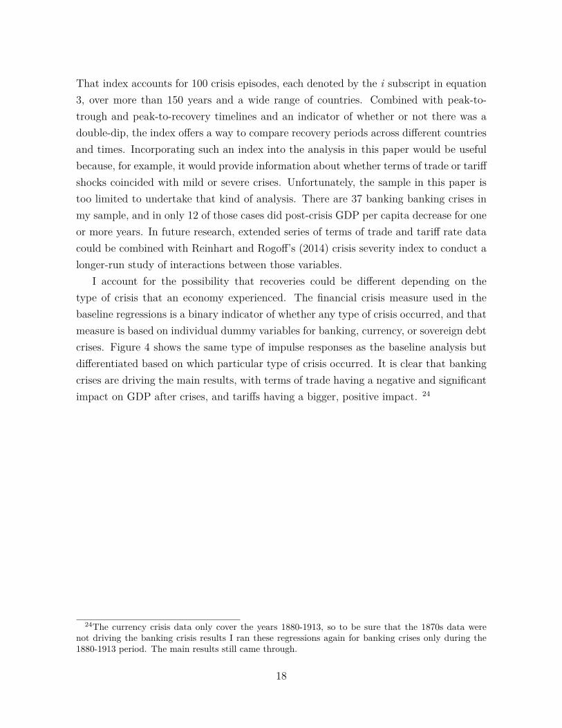
I account for the possibility that recoveries could be different depending on thetype of crisis that an economy experienced. The financial crisis measure used in thebaseline regressions is a binary indicator of whether any type of crisis occurred, and thatmeasure is based on individual dummy variables for banking, currency, or sovereign debtcrises. Figure 4 shows the same type of impulse responses as the baseline analysis butdifferentiated based on which particular type of crisis occurred. It is clear that bankingcrises are driving the main results, with terms of trade having a negative and significantimpact on GDP after crises, and tariffs having a bigger, positive impact. 24

24The currency crisis data only cover the years 1880-1913, so to be sure that the 1870s data werenot driving the banking crisis results I ran these regressions again for banking crises only during the1880-1913 period. The main results still came through.

18

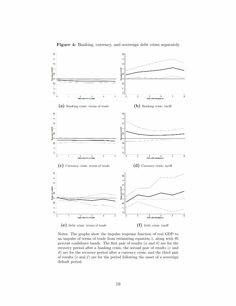
Figure 4: Banking, currency, and sovereign debt crises separately

(a) Banking crisis: terms of trade (b) Banking crisis: tariff

(c) Currency crisis: terms of trade (d) Currency crisis: tariff

(e) Debt crisis: terms of trade (f) Debt crisis: tariff

Notes: The graphs show the impulse response function of real GDP toan impulse of terms of trade from estimating equation 1, along with 95percent confidence bands. The first pair of results (a and b) are for therecovery period after a banking crisis, the second pair of results (c andd) are for the recovery period after a currency crisis, and the third pairof results (e and f ) are for the period following the onset of a sovereigndefault period.

19

I also run different econometric tests to be assured that the results are not undulydriven by the choice of model. The OLS regressions in table 3 test the general relation-ship between five-year averages of GDP per capita growth and the independent variables:terms of trade and tariffs. Using five-year averages of the data follows the growth regres-sion conventions employed by Blattman et al. (2007). It also addresses the concern thatthe annual historical data are imperfect (e.g., with interpolation used to estimate datafor missing years), so averaging captures broader trends. These regressions also includestandard growth regression variables such as initial per capita income, human capital,and population growth measures, along with country and period fixed effects. UsingGDP per capita data here also serves as a robustness check for the baseline analysiswhich used GDP data, by accounting for the population of each country.

Table 3: OLS regressions

Dependent variable:GDP per capita growth

(1) (2) (3) (4) (5) (6)Period: (Whole) (Post-crisis) (Whole) (Post-crisis) (Whole) (Post-crisis)

Terms of trade 0.0000 0.0001 0.0001 0.0001(0.0001) (0.0003) (0.0001) (0.0003)

Terms of trade volatility -0.0006 -0.0013(0.0005) (0.0013)

Terms of trade growth 0.0940* 0.2395(0.0486) (0.1933)

Tariff 0.0003 0.0013* 0.0003 0.0014** 0.0004 0.0015*(0.0003) (0.0007) (0.0003) (0.0007) (0.0003) (0.0008)

Controls Yes Yes Yes Yes Yes YesCountry fixed effects Yes Yes Yes Yes Yes YesPeriod fixed effects Yes Yes Yes Yes Yes YesObservations 315 80 315 80 288 70Number of countries 35 30 35 30 32 27Notes: Robust standard errors in parentheses. Independent variables are lagged. Constant term is included in theregressions but omitted from the table for brevity. Controls include logged initial GDP per capita, the proportion ofthe population with primary schooling, and population growth. * p<0.10, ** p<0.05, *** p<0.01.

Each pair of regressions in table 3 follows the same pattern: the first column of eachpair (1, 3, and 5) includes the whole sample period, and the second column of each pair(2, 4, and 6) is limited to five-year periods that had 60 percent or more of the years

20

during that period identified as post-crisis years.25 Regressions 1 and 2 use the sameterms of trade and tariff measures as the baseline regressions, and the results suggest apositive and significant association between tariffs and growth during post-crisis periods.Regressions 3 and 4 follow Blattman et al. (2007) by using a Hodrick–Prescott filterto isolate the volatility and growth components of terms of trade. Blattman et al.find terms of trade volatility be negatively and significantly associated with economicgrowth in a similar set of countries from 1870-1939. They also find that while termsof trade growth was mostly positively associated with crises, that relationship was notstatistically significant. Regressions 3 and 4 in table 3 control for terms of trade volatilityand growth separately, following the analysis of Blattman et al., in case that is animportant part of explaining growth in post-crisis periods in particular. But that doesnot appear to be the case. The results in regression 4 suggest that tariffs are still moresignificantly associated with post-crisis growth than is any measure of terms of tradechanges.

Regressions 5 and 6 are the same as 1 and 2 but exclude Austria-Hungary, Italy,and the United States, which Blattman et al. identify as part of the industrial core.The results are essentially unchanged, suggesting that the particular core-periphery dis-tinction adopted in this analysis is not what is driving the results. It could also beimportant to differentiate between countries that were price-makers versus price-takersin global commodity markets. Blattman et al. (2007, p. 169) identify Australia, Brazil,Chile, China, India, the Philippines, and Russia as either (1) producing more than fivepercent of world exports, or (2) accounting for more than one-third of the global exportsof a particular commodity. When these countries are dropped from the baseline OLSspecifications (that used in columns 1 and 2 of table 3) the signs and magnitudes of thepost-crisis results are essentially unchanged but the tariff result is no longer significant.But the sample size in that case is down to 64 observations and 24 groups, which couldbe driving that particular result.

In addition to distinguishing between various definitions of core versus peripheralcountries, it is also important to acknowledge that different countries produced differenttypes of exports. Terms of trade fluctuations could thus impact certain sub-samples

25Just as with the baseline regressions, a post-crisis period is defined as the five years after thebeginning of a financial crisis. The data used in the table 3 regressions are averaged in five-yearintervals. The selected inclusion criterion in regressions 2, 4, and 6 is that 60 percent of the years ineach five-year period must be post-crisis years. If that criterion is set at 100 percent the sample is toosmall to undertake this analysis. If it is set at 80 percent the signs of the results are the same, but thetariff result is not significant.

21

of countries differently based on whether they were exporting particular commoditiesat a given time. Countries’ resources and commodity production could be determinedby factors such as geography, chance, or institutions, and later stages of developmentcould be impacted by which commodities were produced in a country. Diaz-Alejandro(1984) dubs this the “commodity lottery” (see also Blattman et al. 2007, p. 160).Similarly, Lewis (1978a, pp. 14-20) highlights the differences between the terms of tradein temperate versus tropical countries, focusing on price differences between temperateand tropical commodities, and how they influenced wages, immigration, and overalldevelopment.26

To test whether Lewis’s distinction between temperate and tropical countries madea difference for how countries recovered from financial crises, the same local projec-tion method is used as for the baseline analysis (equation 1), but the sample is dividedinto temperate and tropical countries, trying several variations of these categories. Onebroad way to categorize the countries in this sample is a temperate versus tropical dis-tinction based on whether countries were temperate grain producers or producers oftropical commodities (Lewis, 1978b, p. 188; Lewis, 1978a, p. 14; these distinctionsgenerally fit with standard geographical definitions of temperate versus tropical regions,based on distance from the equator). Under these guidelines, the temperate countriesinclude those in the European periphery, regions of recent settlement, and the South-ern Cone countries of South America: Argentina, Australia, Austria-Hungary, Canada,Chile, Denmark, Greece, Italy, New Zealand, Norway, Portugal, Russia, Serbia, Spain,Sweden, Turkey, United States, Uruguay. I classify the rest of the countries in the sampleas tropical: Brazil, Burma, Ceylon, China, Colombia, Cuba, Egypt, India, Indonesia,Japan, Mexico, Peru, Philippines, Thailand. The results of this analysis are shown infigure 5.27

26An important factor in Lewis’s analysis is the temperate versus tropical country wage differential.Temperate countries produced commodities which had prices high enough to attract European immi-grants, versus tropical countries which produced commodities whose production paid low wages, due tolow productivity in domestic agriculture (Lewis, 1978a, p. 14).

27Average tariff and terms of trade estimates for each group (tropical and temperate countries) areshown in figure A.1 in the data appendix. Lewis (1978b, p. 14) differentiates more narrowly among“new countries of temperate settlement” (Argentina, Australia, Canada, Chile, New Zealand, and SouthAfrica), the United States, and other (tropical) destinations for European migrants. Lewis (1978b, p.160) explicitly identifies “India, Ceylon, Indonesia, Egypt, Brazil, and other Latin American countries”as being tropical.

22

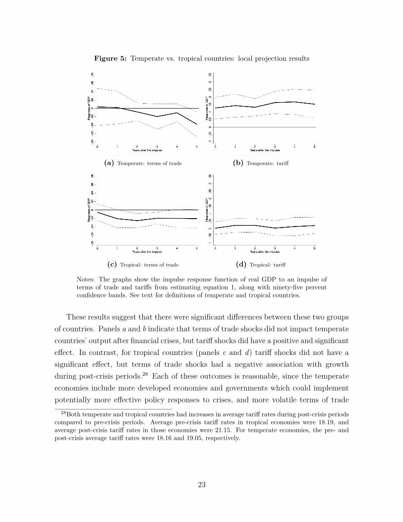
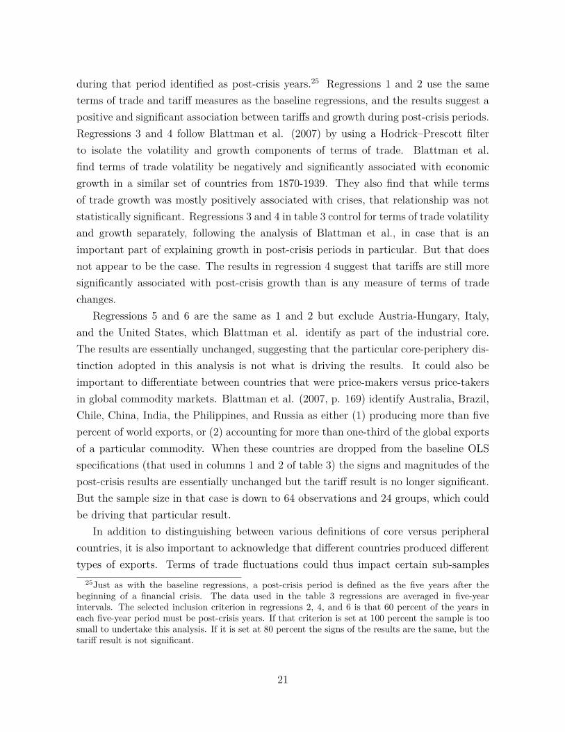
Figure 5: Temperate vs. tropical countries: local projection results

(a) Temperate: terms of trade (b) Temperate: tariff

(c) Tropical: terms of trade (d) Tropical: tariff

Notes: The graphs show the impulse response function of real GDP to an impulse ofterms of trade and tariffs from estimating equation 1, along with ninety-five percentconfidence bands. See text for definitions of temperate and tropical countries.

These results suggest that there were significant differences between these two groupsof countries. Panels a and b indicate that terms of trade shocks did not impact temperatecountries’ output after financial crises, but tariff shocks did have a positive and significanteffect. In contrast, for tropical countries (panels c and d) tariff shocks did not have asignificant effect, but terms of trade shocks had a negative association with growthduring post-crisis periods.28 Each of these outcomes is reasonable, since the temperateeconomies include more developed economies and governments which could implementpotentially more effective policy responses to crises, and more volatile terms of trade

28Both temperate and tropical countries had increases in average tariff rates during post-crisis periodscompared to pre-crisis periods. Average pre-crisis tariff rates in tropical economies were 18.19, andaverage post-crisis tariff rates in those economies were 21.15. For temperate economies, the pre- andpost-crisis average tariff rates were 18.16 and 19.05, respectively.

23

could have a more significant negative impact on less developed tropical countries.29

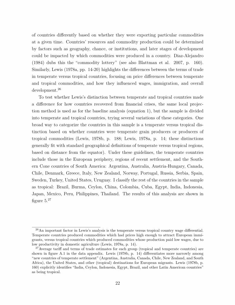
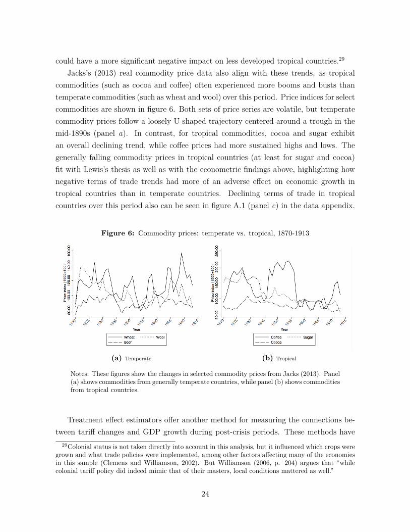
Jacks’s (2013) real commodity price data also align with these trends, as tropicalcommodities (such as cocoa and coffee) often experienced more booms and busts thantemperate commodities (such as wheat and wool) over this period. Price indices for selectcommodities are shown in figure 6. Both sets of price series are volatile, but temperatecommodity prices follow a loosely U-shaped trajectory centered around a trough in themid-1890s (panel a). In contrast, for tropical commodities, cocoa and sugar exhibitan overall declining trend, while coffee prices had more sustained highs and lows. Thegenerally falling commodity prices in tropical countries (at least for sugar and cocoa)fit with Lewis’s thesis as well as with the econometric findings above, highlighting hownegative terms of trade trends had more of an adverse effect on economic growth intropical countries than in temperate countries. Declining terms of trade in tropicalcountries over this period also can be seen in figure A.1 (panel c) in the data appendix.

Figure 6: Commodity prices: temperate vs. tropical, 1870-1913

(a) Temperate (b) Tropical

Notes: These figures show the changes in selected commodity prices from Jacks (2013). Panel(a) shows commodities from generally temperate countries, while panel (b) shows commoditiesfrom tropical countries.

Treatment effect estimators offer another method for measuring the connections be-tween tariff changes and GDP growth during post-crisis periods. These methods have

29Colonial status is not taken directly into account in this analysis, but it influenced which crops weregrown and what trade policies were implemented, among other factors affecting many of the economiesin this sample (Clemens and Williamson, 2002). But Williamson (2006, p. 204) argues that “whilecolonial tariff policy did indeed mimic that of their masters, local conditions mattered as well.”

24

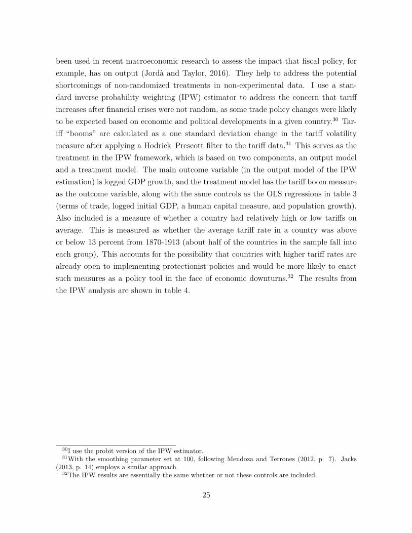
been used in recent macroeconomic research to assess the impact that fiscal policy, forexample, has on output (Jordà and Taylor, 2016). They help to address the potentialshortcomings of non-randomized treatments in non-experimental data. I use a stan-dard inverse probability weighting (IPW) estimator to address the concern that tariffincreases after financial crises were not random, as some trade policy changes were likelyto be expected based on economic and political developments in a given country.30 Tar-iff “booms” are calculated as a one standard deviation change in the tariff volatilitymeasure after applying a Hodrick–Prescott filter to the tariff data.31 This serves as thetreatment in the IPW framework, which is based on two components, an output modeland a treatment model. The main outcome variable (in the output model of the IPWestimation) is logged GDP growth, and the treatment model has the tariff boom measureas the outcome variable, along with the same controls as the OLS regressions in table 3(terms of trade, logged initial GDP, a human capital measure, and population growth).Also included is a measure of whether a country had relatively high or low tariffs onaverage. This is measured as whether the average tariff rate in a country was aboveor below 13 percent from 1870-1913 (about half of the countries in the sample fall intoeach group). This accounts for the possibility that countries with higher tariff rates arealready open to implementing protectionist policies and would be more likely to enactsuch measures as a policy tool in the face of economic downturns.32 The results fromthe IPW analysis are shown in table 4.

30I use the probit version of the IPW estimator.31With the smoothing parameter set at 100, following Mendoza and Terrones (2012, p. 7). Jacks

(2013, p. 14) employs a similar approach.32The IPW results are essentially the same whether or not these controls are included.

25

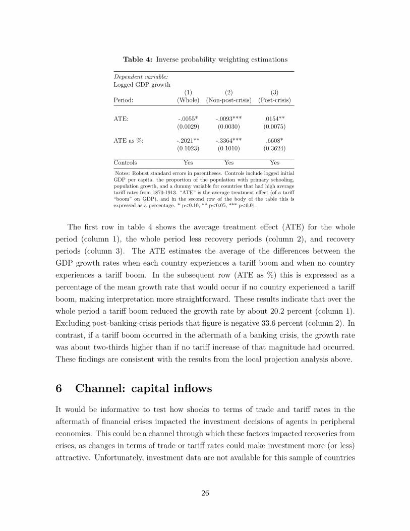
Table 4: Inverse probability weighting estimations

Dependent variable:Logged GDP growth

(1) (2) (3)Period: (Whole) (Non-post-crisis) (Post-crisis)

ATE: -.0055* -.0093*** .0154**(0.0029) (0.0030) (0.0075)

ATE as %: -.2021** -.3364*** .6608*(0.1023) (0.1010) (0.3624)

Controls Yes Yes YesNotes: Robust standard errors in parentheses. Controls include logged initialGDP per capita, the proportion of the population with primary schooling,population growth, and a dummy variable for countries that had high averagetariff rates from 1870-1913. “ATE” is the average treatment effect (of a tariff“boom” on GDP), and in the second row of the body of the table this isexpressed as a percentage. * p<0.10, ** p<0.05, *** p<0.01.

The first row in table 4 shows the average treatment effect (ATE) for the wholeperiod (column 1), the whole period less recovery periods (column 2), and recoveryperiods (column 3). The ATE estimates the average of the differences between theGDP growth rates when each country experiences a tariff boom and when no countryexperiences a tariff boom. In the subsequent row (ATE as %) this is expressed as apercentage of the mean growth rate that would occur if no country experienced a tariffboom, making interpretation more straightforward. These results indicate that over thewhole period a tariff boom reduced the growth rate by about 20.2 percent (column 1).Excluding post-banking-crisis periods that figure is negative 33.6 percent (column 2). Incontrast, if a tariff boom occurred in the aftermath of a banking crisis, the growth ratewas about two-thirds higher than if no tariff increase of that magnitude had occurred.These findings are consistent with the results from the local projection analysis above.

6 Channel: capital inflows

It would be informative to test how shocks to terms of trade and tariff rates in theaftermath of financial crises impacted the investment decisions of agents in peripheraleconomies. This could be a channel through which these factors impacted recoveries fromcrises, as changes in terms of trade or tariff rates could make investment more (or less)attractive. Unfortunately, investment data are not available for this sample of countries

26

for 1870-1913.33 An imperfect substitute is data on capital inflows from Britain (Stone,1999).34 Using these data, Blattman, Hwang, and Williamson (2007) find the samenegative relationship between British capital exports and terms of trade volatility as theyfind for the connection between GDP growth and terms of trade volatility, suggestingthat countries with more volatile terms of trade were less attractive to foreign investors.Also, using annual data and analyzing the “pull factors” that attracted capital flows toperipheral economies over this period, Clemens and Williamson (2004a) find a positiveand significant association between tariff rates and capital inflows, indicating that moreprotectionist trade regimes were attractive to foreign investors. For terms of trade theirresults are also positive, but smaller in magnitude and not statistically significant.

I undertook a similar analysis using the framework developed in this paper, withcapital inflows as the dependent variable (instead of GDP) in equation 1. The resultswere inconclusive, but generally indicate that terms of trade or tariff shocks were notsignificantly associated with capital inflows during post-crisis periods. Over five-yearpost-crisis periods, the coefficient estimates for tariffs were generally of greater magni-tude than the result for terms of trade, and the tariff results mostly had the expectedpositive signs.35 However, the results were not consistently statistically significant. Ialso disaggregated the capital inflow data into capital flows to governments and capitalsflows to private sector industries, and again the results suggest that there is generallyno significant relationship between terms of trade or tariffs and capital inflows (of ei-ther type – government or private sector) during the five-year post-crisis periods. Inthe longer run, capital inflows have been shown to be positively associated with outputgrowth (Bordo and Meissner, 2011). In contrast, the general trends of my findings sug-gest that capital flows were not a major factor contributing to recoveries from financialcrises over this period.

A limitation of my analysis is that foreign capital inflows only account for a fraction ofinvestment in these peripheral economies at this time. Domestic investment was moreimportant for much of the business activity that was undertaken by farms and smallfirms. A one-off commodity price boom could provide farmers, for example, with extramoney to invest in new equipment and expanded production or land acquisition (White,

33Data on investment rates are available for later periods, such as from 1960 onward as presentedin the Penn World Tables, but unfortunately no comparable cross-country data exist for the pre-1913period. The Jordà-Schularick-Taylor Macrohistory Database has investment-to-GDP ratios for only asubsample of the countries covered here.

34Data on capital exports from Germany and France are available from Esteves (2007) and Esteves(2011, 2015), respectively, but only from the early 1880s onward.

35The figures showing these local projection results are omitted here but are available upon request.

27

1982, pp. 80-81). Similarly, firms could finance investment through retained earnings.These avenues of domestic investment are not accounted for in the international capitalflow data. The Jordà-Schularick-Taylor Macrohistory Database has investment-to-GDPratios for nine of the countries in this sample. Local projections (equation 1) using thissubsample and the investment-to-GDP ratio as the dependent variable yield generallyinsignificant results. The same is the case when a measure of domestic investment isgenerated by multiplying the investment-to-GDP ratio by GDP. But this subsample isvery limited, and mostly focuses on the richer/bigger economies from the sample, so Ido not place too much emphasis on these results. They do not convincingly rule out thepossibility that domestic investment increased as a result of terms of trade or tariff ratechanges.

7 Conclusion

This paper addresses two related literatures that look at (1) the connection betweenterms of trade movements and economic growth, and (2) tariff rates and economicgrowth. While the relationship between terms of trade and GDP growth has been clearlydemonstrated (Blattman et al., 2007), finding a connection, if any, between tariffs andgrowth has been more contentious. By focusing specifically on post-crisis periods, thequestion addressed in this paper is more narrow. For post-crisis periods, I find a negativeimpact of terms of trade shocks, but a positive impact for tariff shocks. This suggeststhat national governments played a more active role in shaping economic outcomes thanhas often been appreciated for this period.

This period has traditionally been characterized as being the historical zenith oflaissez-faire capitalism. Focusing on the role of national governments in these economiesat this time challenges this narrative. A growing literature is developing this line ofresearch, finding more evidence for government actions in economies at the dawn of theprogressive era.36 The debates in the United States after the 1893 panic are a prominentexample of these trends.37 A Democratic presidency overlapped with the mid-1890sdepression and the implementation of more liberalized trade policies from 1894-97. This

36See Palen (2015, p. 161) for a summary of the literature that frames the turn of the twentiethcentury as being laissez-faire, as well as the research that refutes that characterization. See also Pollard(1981, p. 252) for a discussion of government interference in trade from 1870-1914.

37A case study of this episode is developed in another chapter of my dissertation. See also Bent(2015a), where I look more closely at the intentions behind trade policy at this time, especially in thecontext of financial crises.

28

allowed protectionist-minded Republicans to assert that free trade policies prolonged thedepression. They argued that protectionist policies would renew confidence in domesticindustry and balance the federal budget through increased tariff revenues. After theRepublican William McKinley assumed the presidency in 1897, tariff rates were raisedto some of the highest levels ever seen in the United States. In that same year, theU.S. economy also began to recover from the mid-1890s depression (the most severedepression through that point in U.S. history). This allowed protectionists to claim thattheir higher tariff rates were indeed effective for spurring output growth in the face of adeep economic downturn.

The validity of those claims is explored elsewhere (Bent 2015a), but this episodeoffers an example of the debates that were taking place at this time over the appropriaterole for policy action to deal with crises. This historical antecedent to the well-studiedpolicy actions taken during the Great Depression38 is under-appreciated, and shapes adeveloping view of the “laisse-faire” turn of the twentieth century as actually having moregovernment involvement in shaping economies after financial crises than has traditionallybeen recognized.

This paper presents a broad cross-country analysis of the interactions between gov-ernments and markets. Its findings suggest that trade policy changes were more impor-tant than terms of trade shocks for explaining renewed economic growth after financialcrises during the globally-integrated 1870-1913 period. As Irwin (2002b) has demon-strated, case studies of this issue can highlight shortcomings in broader cross-countryeconometric studies. The third chapter of my dissertation will provide case studies ofthe United States and Argentina in the 1890s. Further research can look more closely atother individual cases when terms of trade movements and tariff rate changes occurredafter crises. Future research can also explore the investment channel in greater depth asmore data becomes available for measuring domestic investment over this period.

38The literature on policy actions to combat the Great Depression is extensive and has been evolvingsince the 1930s. A relatively recent overview of this literature is presented in Crafts and Fearon (2013).

29

References

Allen, Robert C. (2011). Global Economic History: A Very Short Introduction. Oxford:Oxford University Press.

Amsden, Alice H. (1989). Asia’s Next Giant: South Korea and Late Industrialization.New York: Oxford University Press.

Andrew, A. Piatt (1906). “The Influence of the Crops Upon Business in America.”Quarterly Journal of Economics 20.3, pp. 323–352.

Auernheimer, Leonardo and Susan Mary George (1997). “Shock versus Gradualism inModels of Rational Expectations: The Case of Trade Liberalization.” Journal ofDevelopment Economics 54, pp. 307–322.

Baldacci, Emanuele, Sanjeev Gupta, and Carlos Mulas-Granados (2009). How Effectiveis Fiscal Policy Response in Systemic Banking Crises? IMF Working Paper No.09/160.

Bastiat, Frédéric (2007). The Bastiat Collection. Second Edition. Auburn, Alabama:Ludwig von Mises Institute.

Basu, Parantap and Darryl Mcleod (1992). “Terms of Trade Fluctuations and Eco-nomic Growth in Developing Economies.” Journal of Development Economics 37.1/2,pp. 89–110.

Becker, Torbjörn and Paolo Mauro (2006). “Output Drops and the Shocks that Matter.”IMF Working Paper, WP/06/172.

Bent, Peter H. (2015a). “The Political Power of Economic Ideas: Protectionism in Turnof the Century America.” Economic Thought 4.2, pp. 68–79.

— (2015b). “The Stabilising Effects of the Dingley Tariff and the Recovery from the1890s Depression in the United States.” In Alex Brown, Andy Burn, and Rob Do-herty (Eds.). Crises in Economic and Social History: A Comparative Perspective.Woodbridge, UK: Boydell Press.

Berg, Andrew, Jonathan D. Ostry, and Jeromin Zettelmeyer (2012). “What MakesGrowth Sustained?” Journal of Development Economics 98.2, pp. 149–166.

Bidarkota, Prasad and Mario J. Crucini (2000). “Commodity Prices and the Terms ofTrade.” Review of International Economics 8.4, pp. 647–666.

Biggs, Michael, Thomas Mayer, and Andreas Pick (2010). Credit and Economic Re-covery: Demystifying Phoenix Miracles. Working Paper. url: https ://ssrn . com/abstract=1595980.

30

Bivens, Josh (2016). “Why is Recovery Taking So Long – and Who’s to Blame?” Eco-nomic Policy Institute. url: http://www.epi .org/publication/why- is - recovery-taking-so-long-and-who-is-to-blame/.

Blattman, Christopher, Jason Hwang, and Jeffrey G. Williamson (2007). “Winners andLosers in the Commodity Lottery: The Impact of Terms of Trade Growth and Volatil-ity in the Periphery, 1870-1939.” Journal of Development Economics 82.1, pp. 156–179.

Bloch, Harry and David Sapsford (2011). “Terms of Trade Movements and the GlobalEconomic Crisis.” International Review of Applied Economics 25.5, pp. 503–517.

Bordo, Michael D. and Christopher M. Meissner (2011). “Foreign Capital, FinancialCrises and Incomes in the First Era of Globalization.” European Review of EconomicHistory 15.1, pp. 61–91.

— (2016). “Fiscal and Financial Crises.” NBER Working Paper No. 22059.Brown, Douglass V. et al. (1968 [1934]). The Economics of the Recovery Program.

Freeport, NY: Books for Libraries Press.Brunnermeier, Markus K. and Isabel Schnabel (2016). “Bubbles and Central Banks: His-

torical Perspectives.” In Michael D. Bordo et al. (Eds.). Central Banks at a Cross-roads: What Can We Learn from History? Cambridge: Cambridge University Press,pp. 493–562.

Calvo, Guillermo A., Alejandro Izquierdo, and Ernesto Talvi (2006). “Sudden Stops andPhoenix Miracles in Emerging Markets.” American Economic Review 96.2, pp. 405–410.

Charles, Léo (2017). A New Empirical Test of the Infant-industry Argument: The Caseof Switzerland Protectionism during the 19th century. Working Paper: Cahiers duGREThA no. 2017-11.

Chouliarakis, George and Tadeusz Gwiazdowski (2017). Regime Change and Recoveryin 1930s Britain. Working Paper. url: https://www.nbp.pl/badania/seminaria/8iv2016.pdf.

Clemens, Michael A. and Jeffrey G. Williamson (2002). Closed Jaguar, Open Dragon:Comparing Tariffs in Latin America and Asia before World War II. NBER WorkingPaper No. 9401.

— (2004a). “Wealth Bias in the First Global Capital Market Boom, 1870-1913.” Eco-nomic Journal 114.495, pp. 304–337.

— (2004b). “Why Did the Tariff-Growth Correlation Change after 1950?” Journal ofEconomic Growth 9.1, pp. 5–46.

31

Crafts, Nicholas and Peter Fearon (2013). The Great Depression of the 1930s: Lessonsfor Today. Oxford: Oxford University Press.

Davis, Joseph H., Christopher Hanes, and Paul W. Rhode (2009). “Harvests and Busi-ness Cycles in Nineteenth-Century America.” Quarterly Journal of Economics 124.4,pp. 1675–1727.

Deaton, Angus (1999). “Commodity Prices and Growth in Africa.” Journal of EconomicPerspectives 13.3, pp. 23–40.

Diaz Alejandro, Carlos F. (1984). “Latin America in the 1930s.” In Rosemary Thorp(Ed.). Latin America in the 1930s: The Role of the Periphery in World Crisis. Lon-don: Palgrave Macmillan, pp. 17–49.

“Dingley Bill Discussed” (March 17, 1897). New York Times.Douglas, Paul H. (1935). Controlling Depressions. New York: W.W. Norton and Co.Easterly, William et al. (1993). “Good Policy or Good Luck? Country Growth Perfor-

mance and Temporary Shocks.” Journal of Monetary Economics 32.3, pp. 459–483.Eggertsson, Gauti B. (2012). “Was the New Deal Contractionary?” American Economic

Review 102.1, pp. 524–555.Esteves, Rui Pedro (2007). Between Imperialism and Capitalism: European Capital Ex-

ports before 1914. Working Paper. url: http://users.ox.ac.uk/~econ0243/Imperialism.pdf.

— (2011). “The Belle Epoque of International Finance: French Capital Exports, 1880-1914.” University of Oxford, Department of Economics, Working Paper Number 534.

— (2015). “Description of New French Capital Calls Series.” Unpublished.Fatás, Antonio and Ilian Mihov (2013). Recoveries. Conference Paper. url: http ://

faculty.insead.edu/fatas/research.html.Ford, A. G. (1956). “Argentina and the Baring Crisis of 1890.” Oxford Economic Papers

8.2, pp. 127–150.Fosu, Augustin Kwasi (2011). Terms of Trade and Growth of Resource Economies: A

Tale of Two Countries. Center for the Study of African Economies, University ofOxford, CSAE Working Paper WPS/2011-09.

Funke, Norbert, Eleonara Granziera, and Patrick A. Imam (2008). Terms of Trade Shocksand Economic Recovery. IMF Working Paper No. 08/36.

Gadea, María Dolores, Ana Gómez-Loscos, and Gabriel Pérez-Quirós (2017). DissectingU.S. Recoveries. Banco de España Documentos de Trabajo No. 1708.

32

Ha, Eunyoung and Myung-Koo Kang (2015). “Government Policy Responses to Finan-cial Crises: Identifying Patterns and Policy Origins in Developing Countries.” WorldDevelopment 68, pp. 264–281.

Hadass, Yael S. and Jeffrey G. Williamson (2003). “Terms-of-Trade Shocks and EconomicPerformance, 1870-1940: Prebisch and Singer Revisited.” Economic Development andCultural Change 51.3, pp. 629–656.

Hausman, Joshua K., Paul W. Rhode, and Johannes F. Wieland (2017). Recovery fromthe Great Depression: The Farm Channel in Spring 1933. NBER Working Paper No.23172.

Imam, Patrick and Gonzalo Salinas (2008). Explaining Episodes of Growth Accelerations,Decelerations, and Collapses in Western Africa. IMF Working Paper No. 08/287.International Monetary Fund.

Irwin, Douglas A. (2001). “Tariffs and Growth in Late Nineteenth Century America.”World Economy 24.1, pp. 15–30.

— (2002a). Did Import Substitution Promote Growth in the Late Nineteenth Century?NBER Working Paper No. 8751.

— (2002b). “Interpreting the Tariff-Growth Correlation of the Late 19th Century.”American Economic Association: Papers and Proceedings 92.2, pp. 165–169.

— (2014). Tariff Incidence: Evidence from U.S. Sugar Duties, 1890-1930. NBER Work-ing Paper No. 20635.

Jacks, David S. (2013). From Boom to Bust: A Typology of Real Commodity Prices inthe Long Run. NBER Working Paper No. 18874.

Jalil, Andrew J. and Gisela Rua (2016). “Inflation Expectations and Recovery in Spring1933.” Explorations in Economic History 62, pp. 26–50.

Jerzmanowski, Michał (2006). “Empirics of Hills, Plateaus, Mountains and Plains: AMarkov-switching Approach to Growth.” Journal of Development Economics 81.2,pp. 357–385.

Jordà, Oscar (2005). “Estimation and Inference of Impulse Responses by Local Projec-tions.” American Economic Review 95.1, pp. 161–182.

Jordà, Òscar and Alan M. Taylor (2016). “The Time for Austerity: Estimating theAverage Treatment Effect of Fiscal Policy.” Economic Journal 126.590, pp. 219–255.

“Jordà-Schularick-Taylor Macrohistory Database.” url: http://www.macrohistory.net/data/.

Krueger, Anne O. (1974). “The Political Economy of the Rent-Seeking Society.” Amer-ican Economic Review 64.3, pp. 291–303.

33

Lampe, Markus and Paul Sharp (2013). “Tariffs and Income: A Time Series Analysis for24 Countries.” Cliometrica 7.3, pp. 207–235.

Lanclos, D. Kent and Thomas W. Hertel (1995). “Endogenous Product Differentiationand Trade Policy: Implications for the U.S. Food Industry.” American Journal ofAgricultural Economics 77.3, pp. 591–601.

Lehmann, Sibylle H. and Kevin H. O’Rourke (2011). “The Structure of Protection andGrowth in the Late Nineteenth Century.” Review of Economics and Statistics 93.2,pp. 606–616.

Lewis, W. Arthur (1978a). The Evolution of the International Economic Order. Prince-ton: Princeton University Press.

— (1978b). Growth and Fluctuations, 1870-1913. London: G. Allen and Unwin.List, Friedrich (1909). The National System of Political Economy. London: Longmans,

Green and Co.Maddison, Angus (1995). Monitoring the World Economy 1820-1992. Paris: OECD De-

velopment Centre.Malakellis, Michael (1998). “Should Tariff Reduction be Announced? An Intertemporal

Computable General Equilibrium Analysis.” Economic Record 74.225, pp. 121–138.“NBER Macrohistory Database, U.S. Index of Composite Wages 1820-1909 (a08061a).”

url: http://www.nber.org/databases/macrohistory/contents/.Novak, William J. (1996). The People’s Welfare: Law and Regulation in Nineteenth-

Century America. Chapel Hill, NC: University of North Carolina Press.— (2008). “The Myth of the ’Weak’ American State.” American Historical Review 113.3,

pp. 752–772.O’Rourke, Kevin H. (2000). “Tariffs and Growth in the Late 19th Century.” Economic

Journal 110.463, pp. 456–483.Owyang, Michael T., Valerie A. Ramey, and Sarah Zubairy (2013). “Are Government

Spending Multipliers Greater during Periods of Slack? Evidence from Twentieth-Century Historical Data.” American Economic Review 103.3, pp. 129–134.

Palen, Marc-William (2015). “The Imperialism of Economic Nationalism, 1890-1913.”Diplomatic History 39.1, pp. 157–185.

Payne, Jonathan and Lawrence Uren (2014). “Economic Policy and the Great Depressionin a Small Open Economy.” Journal of Money, Credit and Banking 46.2-3, pp. 347–370.

Pollard, Sidney (1981). Peaceful Conquest: The Industrialization of Europe 1760-1970.New York: Oxford University Press.

34

Ramey, Valerie A. and Sarah Zubairy (2014). Government Spending Multipliers in GoodTimes and in Bad: Evidence from U.S. Historical Data. NBER Working Paper No.20719.

Reinhart, Carmen M., Vincent Reinhart, and Christoph Trebesch (2016). “Global Cy-cles: Capital Flows, Commodities, and Sovereign Defaults, 1815-2015.” AmericanEconomic Review 106.5, pp. 574–580.

Reinhart, Carmen M. and Kenneth S. Rogoff (2009a). “The Aftermath of FinancialCrises.” American Economic Review 99.2, pp. 466–472.

— (2009b). This Time is Different: Eight Centuries of Financial Folly. Princeton: Prince-ton University Press.

— (2014). “Recovery from Financial Crises: Evidence from 100 Episodes.” AmericanEconomic Review 104.5, pp. 50–55.

Rocha, Bruno and Solomos Solomou (2015). “The Effects of Systemic Banking Crises inthe Inter-War Period.” Journal of International Money and Finance 54, pp. 35–49.

Rodríguez, Francisco and Dani Rodrik (2000). “Trade Policy and Economic Growth: ASceptic’s Guide to the Cross-national Evidence.” In Ben S. Bernanke and KennethRogoff (Eds.). NBER Macroeconomics Annual, Volume 15. Cambridge, MA: MITPress, pp. 261–338.

Rodrik, Dani (1999). “Where Did All the Growth Go? External Shocks, Social Conflict,and Growth Collapses.” Journal of Economic Growth 4.4, pp. 385–412.

Romer, Christina D. and David Romer (2016). “New Evidence on the Impact of FinancialCrises in Advanced Countries.” NBER Working Paper No. 21021.

Sachs, Jeffrey D. and Andrew M. Warner (2001). “The Curse of Natural Resources.”European Economic Review 45.4, pp. 827–838.

Sachs, Jeffrey and Andrew Warner (1995). “Economic Reform and the Process of GlobalIntegration.” Brookings Papers on Economic Activity 1, pp. 1–118.

Schularick, Moritz and Solomos Solomou (2011). “Tariffs and Economic Growth in theFirst Era of Globalization.” Journal of Economic Growth 16.1, pp. 33–70.

Shelburne, Robert C. (2010). “The Global Financial Crisis and its Impact on Trade: TheWorld and the European Emerging Economies.” United Nations Economic Commis-sion for Europe, Discussion Paper No. 2010.2.

Spearot, Alan (2016). “Unpacking the Long-Run Effects of Tariff Shocks: New Struc-tural Implications from Firm Heterogeneity Models.” American Economic Journal:Microeconomics 8.2, pp. 128–167.

35

Stern, Clarence A. (1971). Protectionist Republicanism: Republican Tariff Policy in theMcKinley Period. Ann Arbor: Edwards Brothers.

Stone, Irving (1999). The Global Export of Capital from Great Britain, 1865-1914: AStatistical Survey. New York: St. Martin’s Press.

Suter, Christian (1990). Schuldenzyklen in der Dritten Welt: Kreditaufnahme, Zahlungskrisenund Schuldenregelungen peripherer Länder im Weltsystem von 1820 bis 1986. Frank-furt am Main: A. Hain.

— (1992). Debt Cycles in the World Economy: Foreign Loans, Financial Crises, andDebt Settlements, 1820-1990. Boulder, CO: Westview Press.

Taylor, Jason E. and Todd C. Neumann (2016). “Recovery Spring, Faltering Fall: Marchto November 1933.” Explorations in Economic History 61, pp. 54–67.

Turnovsky, Stephen J. and Pradip Chattopadhyay (2003). “Volatility and Growth inDeveloping Economies: Some Numerical Results and Empirical Evidence.” Journalof International Economics 59.2, pp. 267–295.

White, G. T. (1939). “Economic Recovery and the Wheat Crop of 1897.” AgriculturalHistory 13.1, pp. 13–21.

— (1982). The United States and the Problem of Recovery after 1893. Tuscaloosa, AL:University of Alabama Press.

Williamson, Jeffrey G. (2006). “Explaining World Tariffs 1870–1938: Stolper-Samuelson,Strategic Tariffs and State Revenues.” In R. Findlay et al. (Eds.). Eli F. Heckscher,International Trade, and Economic History. Cambridge: MIT Press, pp. 199–228.

36

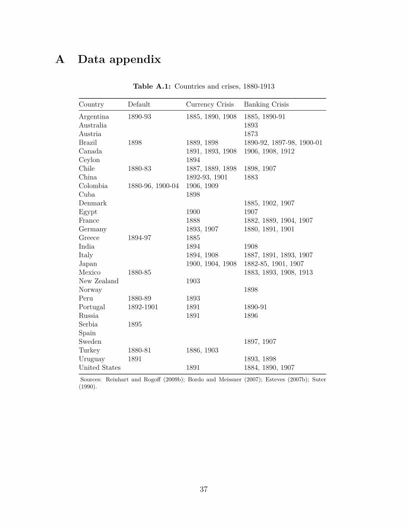
A Data appendix

Table A.1: Countries and crises, 1880-1913

Country Default Currency Crisis Banking CrisisArgentina 1890-93 1885, 1890, 1908 1885, 1890-91Australia 1893Austria 1873Brazil 1898 1889, 1898 1890-92, 1897-98, 1900-01Canada 1891, 1893, 1908 1906, 1908, 1912Ceylon 1894Chile 1880-83 1887, 1889, 1898 1898, 1907China 1892-93, 1901 1883Colombia 1880-96, 1900-04 1906, 1909Cuba 1898Denmark 1885, 1902, 1907Egypt 1900 1907France 1888 1882, 1889, 1904, 1907Germany 1893, 1907 1880, 1891, 1901Greece 1894-97 1885India 1894 1908Italy 1894, 1908 1887, 1891, 1893, 1907Japan 1900, 1904, 1908 1882-85, 1901, 1907Mexico 1880-85 1883, 1893, 1908, 1913New Zealand 1903Norway 1898Peru 1880-89 1893Portugal 1892-1901 1891 1890-91Russia 1891 1896Serbia 1895SpainSweden 1897, 1907Turkey 1880-81 1886, 1903Uruguay 1891 1893, 1898United States 1891 1884, 1890, 1907Sources: Reinhart and Rogoff (2009b); Bordo and Meissner (2007); Esteves (2007b); Suter(1990).

37

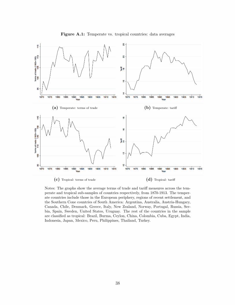
Figure A.1: Temperate vs. tropical countries: data averages

(a) Temperate: terms of trade (b) Temperate: tariff

(c) Tropical: terms of trade (d) Tropical: tariff

Notes: The graphs show the average terms of trade and tariff measures across the tem-perate and tropical sub-samples of countries respectively, from 1870-1913. The temper-ate countries include those in the European periphery, regions of recent settlement, andthe Southern Cone countries of South America: Argentina, Australia, Austria-Hungary,Canada, Chile, Denmark, Greece, Italy, New Zealand, Norway, Portugal, Russia, Ser-bia, Spain, Sweden, United States, Uruguay. The rest of the countries in the sampleare classified as tropical: Brazil, Burma, Ceylon, China, Colombia, Cuba, Egypt, India,Indonesia, Japan, Mexico, Peru, Philippines, Thailand, Turkey.

38