Application Note

irf-mp-04.doc Becker & Hickl GmbH 2008 1

Recording the Instrument Response Function of a Multiphoton FLIM System

Abstract. FLIM data analysis in presence of SHG signals or extremely fast decay components requires the correct instrument response function (IRF) to be used. This application note describes how an accurate IRF is obtained in a multiphoton microscope.

Theoretical Background

A measurement in the FLIM modes of the bh SPC-150 or SPC-830 TCSPC modules delivers the photon distribution over the coordinates of the scan, the time within the fluorescence decay, and, if several detector in different spectral channels are used, the wavelength [1]. The data can be considered an array of pixels, each containing a large number of time channels spread over the fluorescence decay. In other words, the FLIM measurement delivers images with a decay curve in each pixel. Several such arrays may exist if several detectors or a multi-wavelength detector are used.

To obtain fluorescence lifetimes from these data the decay curves in the individual pixels must be fitted with an appropriate model. However, the time resolution of the measurement system is finite. Therefore the fitting routine has to take the ‘instrument response function’ (IRF) into account. The IRF is the pulse shape the FLIM system records for an infinitely short fluorescence lifetime. The fitting procedure convolutes the model function with the IRF and compares the result with the photon numbers in the subsequent time channels of the current pixel. Then it varies the model parameters until the best fit between the convoluted model function and the measured decay data is obtained [7].

At first glance, recording the IRF of a FLIM system may appear easy. The emission filters would be removed or replaced with bandpass filters centred at the laser wavelength, and a scattering signal would be recorded from a scattering target. Unfortunately, recording an accurate IRF in a laser scanning microscope is much more difficult. The obvious problem is that the dichroic beamsplitter of the microscope does not pass the excitation wavelength to the detectors. Moreover, the excitation beam path usually contains a laser blocking filter that cannot easily be removed. In a two-photon microscope it may even happen that the FLIM detector is not sensitive to the excitation wavelength altogether. Of course, by increasing the laser power something is detected in any PMT. However, a photocathode for the visible spectrum is virtually transparent in the NIR, and a large fraction of the photoelectrons may be emitted not from the cathode but from the first dynode. The detector response recorded in the NIR is therefore not necessarily identical with the response at the normal detection wavelength. Moreover, a signal detected at the laser wavelength is usually contaminated by reflections and scattering in the optical system, and by fluorescence from the target [2].

The bh SPCImage and Optispec FLIM data analysis software therefore allows the user to derive an estimated IRF from the fluorescence signal itself. The IRF estimation works at satisfactory accuracy for fluorescence signals with lifetimes a few times longer than the width of the IRF [3, 4, 5]. However, if the fluorescence contains extremely fast components, or if second-harmonic signals are

Application Note

2 irf-mp04.doc

present the IRF estimation fails. For such signals there is no other solution than recording the true IRF of the system.

Recording the IRF in a multiphoton system requires a fast process that transfers the excitation wavelength into the typical wavelength range of the fluorescence. It is often suggested to use a short-lifetime fluorescence to obtain this wavelength conversion. Such attempts usually fail because sufficiently short lifetimes can only be obtained from strongly quenched fluorescence. The fluorescence quantum yield is correspondingly low, and so is the intensity. The slightest amount of contamination with other fluorescent molecules makes the result useless. It is therefore better to use second-harmonic generation (SHG) to convert the wavelength. SHG is an ultrafast nonlinear process that delivers a signal at one half of the excitation wavelength. SHG occurs in materials that have a high degree of order on the molecular scale. Typical examples are collagen fibres and a number of crystals.

Recording an IRF

Strong SHG signals are obtained from urea, (NH2)2CO, or potassium di-hydrogene phosphate (KDP, KH2PO4) micro-crystals. To obtain an SHG target, dissolve urea or KDP in water, place a droplet of solution on a cover slip, and let it dry. Make a few attempts with different concentration. If the concentration is right a thin layer of small crystals remains on the glass. Place the cover slip upside-down on a microscope slide, and you have your IRF target.

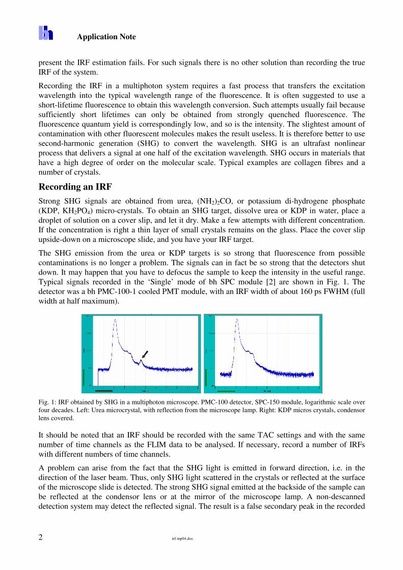
The SHG emission from the urea or KDP targets is so strong that fluorescence from possible contaminations is no longer a problem. The signals can in fact be so strong that the detectors shut down. It may happen that you have to defocus the sample to keep the intensity in the useful range. Typical signals recorded in the ‘Single’ mode of bh SPC module [2] are shown in Fig. 1. The detector was a bh PMC-100-1 cooled PMT module, with an IRF width of about 160 ps FWHM (full width at half maximum).

Fig. 1: IRF obtained by SHG in a multiphoton microscope. PMC-100 detector, SPC-150 module, logarithmic scale over four decades. Left: Urea microcrystal, with reflection from the microscope lamp. Right: KDP micros crystals, condensor lens covered.

It should be noted that an IRF should be recorded with the same TAC settings and with the same number of time channels as the FLIM data to be analysed. If necessary, record a number of IRFs with different numbers of time channels.

A problem can arise from the fact that the SHG light is emitted in forward direction, i.e. in the direction of the laser beam. Thus, only SHG light scattered in the crystals or reflected at the surface of the microscope slide is detected. The strong SHG signal emitted at the backside of the sample can be reflected at the condensor lens or at the mirror of the microscope lamp. A non-descanned detection system may detect the reflected signal. The result is a false secondary peak in the recorded

Application Note

irf-mp-04.doc Becker & Hickl GmbH 2008 3

IRF shape, as it can be seen in Fig. 1, left. It is therefore recommended to put a non-reflective cover over the sample when an IRF is recorded.

An SHG image from an urea sample is shown in Fig. 2. The image was recorded by a bh non-descanned detection system [6] attached to a Leica SP5 MP multiphoton microscope [5]. The main panel of SPCM software was configured to show the image (left) and the waveforms within the first 128 lines of the image (right) [2].

Fig. 2: SHG image of an urea sample, recorded by an SPC-150 NDD FLIM system attached to a Leica SP5 MP microscope. Main panel of SPCM software, configured to show an image and the waveforms within the first 128 lines of the image.

Background Subtraction

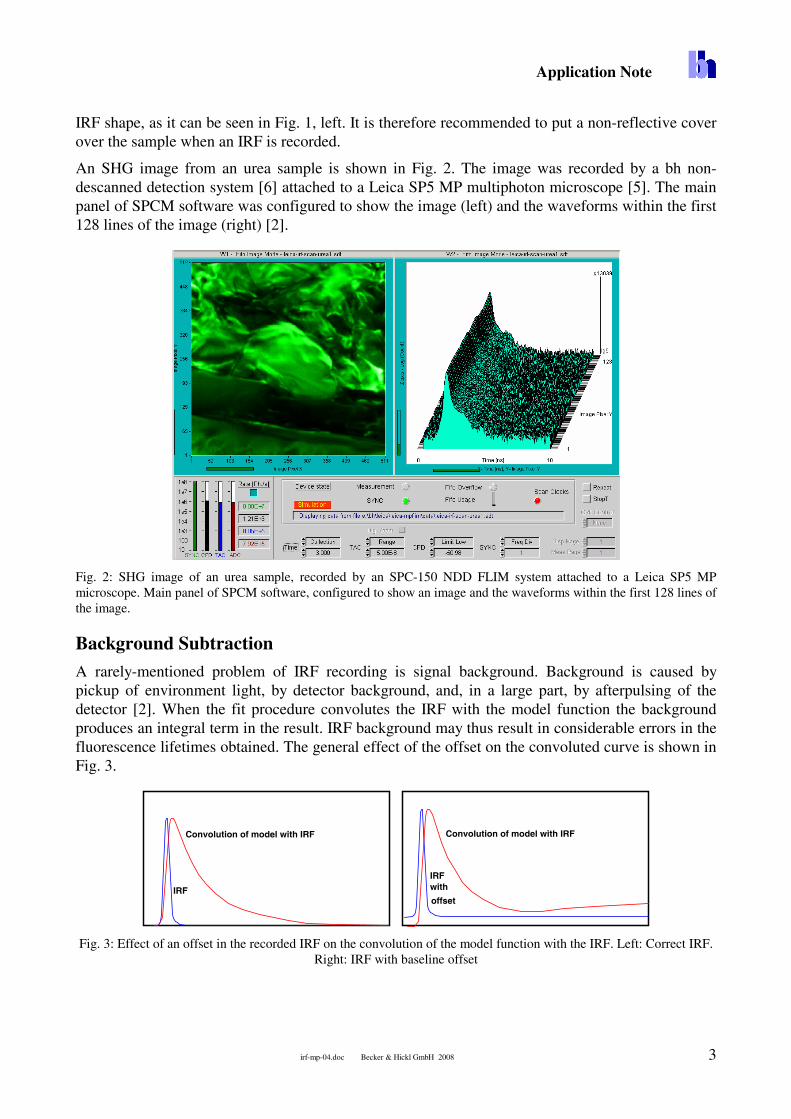
A rarely-mentioned problem of IRF recording is signal background. Background is caused by pickup of environment light, by detector background, and, in a large part, by afterpulsing of the detector [2]. When the fit procedure convolutes the IRF with the model function the background produces an integral term in the result. IRF background may thus result in considerable errors in the fluorescence lifetimes obtained. The general effect of the offset on the convoluted curve is shown in Fig. 3.

IRF

Convolution of model with IRF

IRFwith

offset

Convolution of model with IRF

Fig. 3: Effect of an offset in the recorded IRF on the convolution of the model function with the IRF. Left: Correct IRF.

Right: IRF with baseline offset

Application Note

4 irf-mp04.doc

The IRF background is tolerable if the integral intensity of the background remains less than 1 % of the integral intensity in the IRF peak. Because the IRF peak is much narrower than the recording time interval this can be difficult to achieve. It may therefore be necessary to subtract the background from the IRF recording before the data are used for de-convolution. The operation can be performed by using the data operations of the bh SPCM software [2]. Background subtraction for an IRF recorded in the ‘Single’ mode is shown in Fig. 4. To process the data, click into ‘Display’, ‘2D Curve’. Switch the display parameters to ‘logarithmic’. The resulting 2D Display panel is shown in Fig. 4, left. Activate the cursors and pull the left cursor fully left and down, the right cursor fully right and up. Then click on the ‘Data Processing’ button in the lower right of the 2D curve panel. This opens the data processing panel shown in Fig. 4, right. Select Operation ‘Shift in Y Direction’, and chose a negative constant to shift the data. By clicking on ‘Execute’ the curve is shifted down by an amount given by the constant selected. You may use a small shift constant, and repeat the shift operation until the background is removed. The result can be seen in Fig. 4, right. When the operation is completed return to the main panel and save the IRF data into a file.

Fig. 4: Left: IRF recorded in the ‘Single’ mode of an SPC-150, displayed in the ‘2D Curve Window’. Right: Data Processing panel opened, background subtracted.

If you have recorded the IRF in one of the SPC imaging modes, you may proceed as described below.

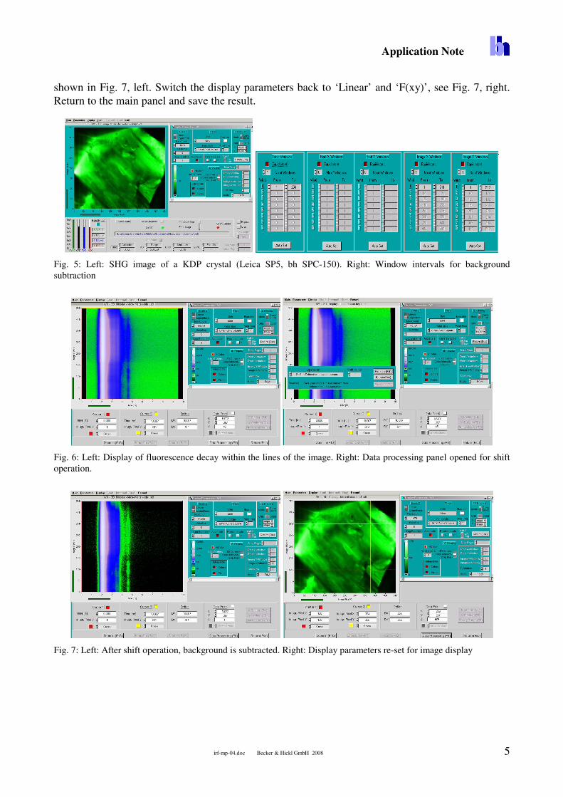
Fig. 5, left, shows an SHG image of a KDP crystal recorded by an SPC-150 module attached to the RLD port of a Leica SP5 MP microscope [6]. When you have recorded an SHG image like the one shown in Fig. 5, save the data by the save routine of the SPCM software. Then open the ‘Window Intervals’ and set the number of ‘time windows’ and image ‘X and Y windows’ to ‘one’. Click on ‘auto set’ to include all time channels and pixels, see Fig. 5, right. (You may leave the Window Intervals like this for the next FLIM measurement).

Then click into ‘Display’, 3D curve. Open the ‘Display parameters’ (if not already open) and set Scale Z to ‘logarithmic’ and Mode to ‘F(t,y)’, see Fig. 6, left. What you see is the combined fluorescence decay within the lines of the image displayed in brightness and false colour. Due to the logarithmic scale, the background is clearly visible. Pull the cursors fully out to the lower left and upper right corners of the image.

Click into ‘Data Processing’, and select ‘Shift in Z Direction’. Select a small negative shift value, see Fig. 6, right. Please note that the required shift is small because it refers to the background counts in the individual time channels of the individual pixels. Therefore, start with a shift value of ‘-1’, and repeat the shift operation if necessary. Click into ‘Execute’ until you obtain a result as

Application Note

irf-mp-04.doc Becker & Hickl GmbH 2008 5

shown in Fig. 7, left. Switch the display parameters back to ‘Linear’ and ‘F(xy)’, see Fig. 7, right. Return to the main panel and save the result.

Fig. 5: Left: SHG image of a KDP crystal (Leica SP5, bh SPC-150). Right: Window intervals for background subtraction

Fig. 6: Left: Display of fluorescence decay within the lines of the image. Right: Data processing panel opened for shift operation.

Fig. 7: Left: After shift operation, background is subtracted. Right: Display parameters re-set for image display

Application Note

6 irf-mp04.doc

Import of an IRF into the SPCImage Data Analysis

Importing an IRF from image data

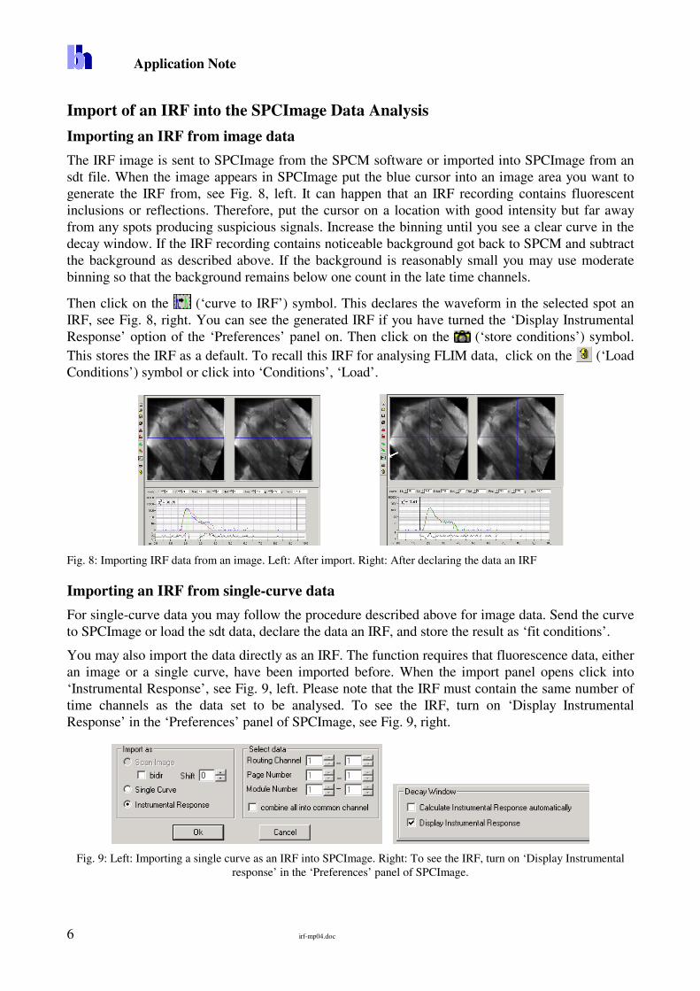
The IRF image is sent to SPCImage from the SPCM software or imported into SPCImage from an sdt file. When the image appears in SPCImage put the blue cursor into an image area you want to generate the IRF from, see Fig. 8, left. It can happen that an IRF recording contains fluorescent inclusions or reflections. Therefore, put the cursor on a location with good intensity but far away from any spots producing suspicious signals. Increase the binning until you see a clear curve in the decay window. If the IRF recording contains noticeable background got back to SPCM and subtract the background as described above. If the background is reasonably small you may use moderate binning so that the background remains below one count in the late time channels.

Then click on the (‘curve to IRF’) symbol. This declares the waveform in the selected spot an IRF, see Fig. 8, right. You can see the generated IRF if you have turned the ‘Display Instrumental Response’ option of the ‘Preferences’ panel on. Then click on the (‘store conditions’) symbol. This stores the IRF as a default. To recall this IRF for analysing FLIM data, click on the (‘Load Conditions’) symbol or click into ‘Conditions’, ‘Load’.

Fig. 8: Importing IRF data from an image. Left: After import. Right: After declaring the data an IRF

Importing an IRF from single-curve data

For single-curve data you may follow the procedure described above for image data. Send the curve to SPCImage or load the sdt data, declare the data an IRF, and store the result as ‘fit conditions’.

You may also import the data directly as an IRF. The function requires that fluorescence data, either an image or a single curve, have been imported before. When the import panel opens click into ‘Instrumental Response’, see Fig. 9, left. Please note that the IRF must contain the same number of time channels as the data set to be analysed. To see the IRF, turn on ‘Display Instrumental Response’ in the ‘Preferences’ panel of SPCImage, see Fig. 9, right.

Fig. 9: Left: Importing a single curve as an IRF into SPCImage. Right: To see the IRF, turn on ‘Display Instrumental

response’ in the ‘Preferences’ panel of SPCImage.

Application Note

irf-mp-04.doc Becker & Hickl GmbH 2008 7

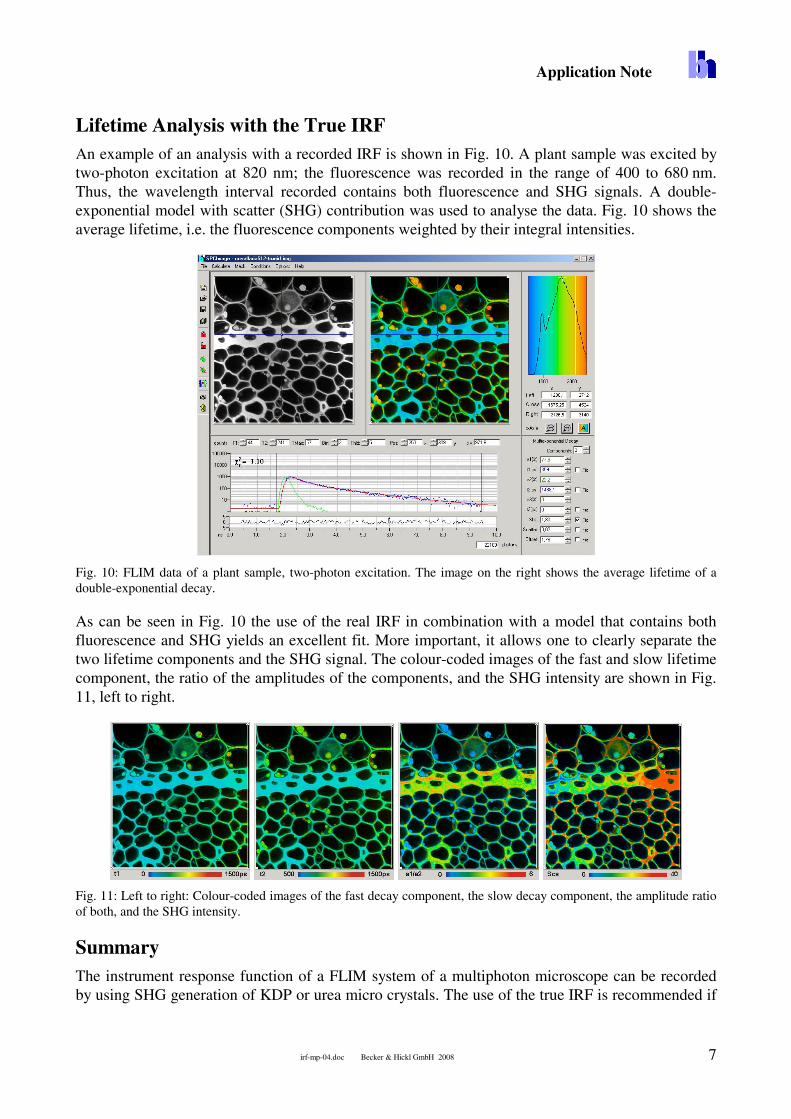
Lifetime Analysis with the True IRF An example of an analysis with a recorded IRF is shown in Fig. 10. A plant sample was excited by two-photon excitation at 820 nm; the fluorescence was recorded in the range of 400 to 680 nm. Thus, the wavelength interval recorded contains both fluorescence and SHG signals. A double-exponential model with scatter (SHG) contribution was used to analyse the data. Fig. 10 shows the average lifetime, i.e. the fluorescence components weighted by their integral intensities.

Fig. 10: FLIM data of a plant sample, two-photon excitation. The image on the right shows the average lifetime of a double-exponential decay.

As can be seen in Fig. 10 the use of the real IRF in combination with a model that contains both fluorescence and SHG yields an excellent fit. More important, it allows one to clearly separate the two lifetime components and the SHG signal. The colour-coded images of the fast and slow lifetime component, the ratio of the amplitudes of the components, and the SHG intensity are shown in Fig. 11, left to right.

Fig. 11: Left to right: Colour-coded images of the fast decay component, the slow decay component, the amplitude ratio of both, and the SHG intensity.

Summary The instrument response function of a FLIM system of a multiphoton microscope can be recorded by using SHG generation of KDP or urea micro crystals. The use of the true IRF is recommended if

Application Note

8 irf-mp04.doc

a sample delivers fast signals, such as an extremely fast decay component or SHG signals. A model containing several lifetime components and an SHG component can e used to derive the lifetimes of the components, the intensity coefficients, and the SHG intensity.

References 1. W. Becker, Advanced time-correlated single-photon counting techniques. Springer, Berlin, Heidelberg, New York,

2005 2. W. Becker, The bh TCSPC handbook. Becker & Hickl GmbH (2005), www.becker-hickl.com 3. Becker & Hickl GmbH, DCS-120 Confocal Scanning FLIM Systems, user handbook. www.becker-hickl.com 4. Becker & Hickl GmbH, Modular FLIM systems for Zeiss LSM 510 and LSM 710 laser scanning microscopes. User

handbook. Available on www.becker-hickl.com 5. Becker & Hickl GmbH and Leica Microsystems, Leica MP-FLIM and D-FLIM Fluorescence Lifetime Microscopy

Systems. User handbook. Available on www.becker-hickl.com 6. bh NDD FLIM systems for Leica SP2 MP and SP5 MP Multiphoton Microscopes. Application note, Becker & Hickl

GmbH (2007), www.becker-hickl.com 7. D.V. O’Connor, D. Phillips, Time-correlated single photon counting, Academic Press, London (1984)