RECORD, Volume 28, No. 1* - Society of Actuaries

_________________________________ *Copyright © 2002, Society of Actuaries

†Mr. Robert N. Roseman, not a member of the sponsoring organizations, is director, insurance of Ratings/Capital Markets at Standards and Poor's in New York, NY. Note: The chart(s) referred to in the text can be found at the end of the manuscript.

RECORD, Volume 28, No. 1*

Colorado Springs Spring Meeting May 30-31, 2002 Session 19TS S&P Financial Products Company Model Track: Investment Moderator: MR. CRAIG FOWLER Panelists: MS. ELLEN WOODRUFF HALL MR. ROBERT N. ROSEMAN†

Summary: Attendees learn about the new capital allocation, the financial products company (FPC) model recently developed by S&P, including S&P's view of interest rate risk and credit risk in the FPC model, challenges of implementing the model for a life insurance company and learn how the FPC model compares to economic capital methodology. MR. ROBERT N. ROSEMAN: My name is Bob Roseman, I'm a director at Standard & Poor's, and I'm going to be talking about applying Standard & Poor's financial product company model to insurance companies. The model was developed several years ago, and we originally developed it to apply to the derivative product company and financial product company subsidiaries of insurance companies, which would include AIG Financial Products or Gen-Re Financial Products. About a year ago, we thought it would make sense to start applying it to certain portions of insurance companies. The model that I'm going to go through is actually sort of a stripped-down version of the model that we apply to the derivative product companies. There are certain things that typically insurance companies aren't involved in, like writing over-the-counter (OTC) derivatives, options and things like that. So, we exclude some of the charges. We developed a model and got quite a bit of feedback from the risk managers at

S&P Financial Products Company Model 2 these derivative product companies. In the future, I would expect to get feedback from companies like yours. We view it as a starting point, and we continuously modify the model. Basically, we have to modify it somewhat for each company we look at. Before coming to Standard & Poor's, I actually ran spread business for AMBAC. One of the sources of frustration for me was the capital charge that Standard & Poor's assessed to my business. I would have been happy to have this then, so hopefully it can add some value to some of your companies. The objectives of the presentation are fourfold:

1. We want to create an awareness of the opportunity that we're presenting to apply our financial product model to insurance companies.

2. We want to provide a basic conceptual understanding of the model to this audience.

3. Most important, we want to illustrate the value that the model can provide for companies seeking to optimize their capital reserves.

4. And last, we're going to go illustrate some advanced risk management techniques that are currently being applied to insurance companies.

I'm going to talk about Standard & Poor's rationale for applying the model. I'm going to talk about some potential applications of the model. We're going to talk about the qualifying characteristics for applying the model to your company. We're going to go through an overview of the model. And probably the best thing we're going to do is go through an illustrated application to a sample GIC portfolio. The last thing we're going to do is compare the capital charge that we would get using this model relative to our traditional model. Why This Model? We decided to apply this model to the insurance companies because part of it has to do with the increased sophistication of risk management practices that are currently being employed in insurance companies. Over the last five or six years we've seen quite a few insurance companies adopting the type of risk management processes that were traditionally used at banks and derivative product companies. This model allows us to factor that into our analysis of your companies. We've also seen an increased pressure on insurance companies to optimize their capital base. This model allows companies to do that. Over the years we get quite a few inquiries from companies saying, "We do a great job of managing our risk, and we're using this hedging strategy and that hedging strategy. How can we reflect that in our capital adequacy?" This model gives us a tool to be able to do that.

S&P Financial Products Company Model 3 We've also seen an increase in the volume of operational leverages—quite a few insurance companies are issuing GICs or medium-term note programs. And this is an excellent tool for us to analyze that. Typically I don't view a lot of them, but there is quite a bit of risk in this business. And this model ferrets that out and provides the correct amount of capital against it. Potential Applications Some of the potential applications for this model: We apply it to the noninsurance books of insurance companies. If based for pure insurance risk, we still have to use our traditional model, but we would use this for GIC books, medium-term note programs or credit derivatives. Once again, it allows us to quantify risk mitigation strategies, such as OTC derivatives or credit derivatives. We've also used it for certain companies that have come to us and aren't using the model for the rest of their company, and they want to do it. They have a specific large-structured transaction or something that they're doing that this model makes sense for, and we're willing to do that. We've also used it for financial product company subsidiaries. We've had companies that want to set up credit derivative vehicles and so forth. We would do that, or if companies want to do an enhanced vehicle, we could use this model to determine the amount of capital that would be held against the business. And last, it gives us a good way to designate operational leverages, match-funded, so it doesn't get included in your financial leverage ratios. Say you're an AA company and you want to be an AAA company, and you wanted to set up a special purpose vehicle. You want to over-capitalize it or do a joint probability, or you get somebody else to wrap you like a single A wraps the SPV (special purpose vehicle) over the insurance company. We could use this to say, "OK, it's not an AA company anymore; it's AAA. How much capital should be against that?" Frankly, in general I don't think that many insurance companies have explored ways of doing that. Certainly, if I wasn't at Standard & Poor's, one of the first things that I would do is that trade. I probably would look for ways to create a capital-efficient way to create an enhanced vehicle, especially in the institutional spread business. Qualifying Characteristics In order for us to apply the model to a company, there are certain qualifying characteristics: First and foremost, you have to have comprehensive and sophisticated risk management that's consistent with the model. I've had companies come and say, "We duration–match," and things like that. That's not

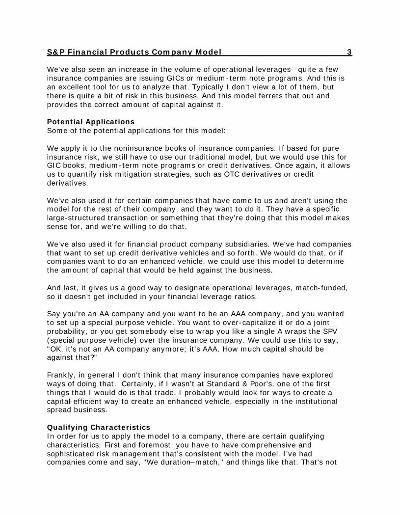
S&P Financial Products Company Model 4 going to give us the type of resolution that we need to potentially decrease your capital adequacy. And we'd also expect you to have a more conservative market or credit risk profile than the market in general. We can apply it to any company, but to really get a benefit from using a model, you'd basically have to be in a situation in which you're more conservative than the industry norm. And this can be accomplished, of course, through advanced hedging strategies or superior underwriting or risk and investment guidelines. And last, you have to be able to separately identify your assets, liabilities and hedge instruments. They don't have to be legally segregated or anything but, you can't just say, "This is 60 percent of our general account assets." The Model In General Basically, the model is broken down into three major sections, which we use to analyze your net credit, market and operational risk. The capital adequacy is determined based on the expected or potential losses from the exposures. It's a little different than our traditional model, which is just a factor-based model that doesn't really have anything to do with what your true exposure is. When we determine the credit risk we determine it based on our Standard & Poor's historical default studies. Financial market risk, in this case, is pretty much strictly interest rate risk as determined by applying interest rate volatilities to the interest rate sensitivities that are supplied by the companies that we're analyzing. Operational risk is determined by various subjective factors that I'm going to discuss. We were attempting to create a statistical level of confidence that we feel is commensurate with the rating category that the company is in. Obviously, the higher the rating category, the higher the statistical level of confidence that we're trying to achieve (Table 1).

S&P Financial Products Company Model 5

Table 1

8Page

FPC Model Overview

• Applied volatilities and default factors create a statistical level of confidence for losses consistent with the rating category

• The higher the rating category, the greater the statistical level of confidence created, for all risk categories

RatingCategory

Std.Deviations Confidence

Capital AdequacyRatio Assessment

AAA 3.00 99.9% 1.75 Extremely Strong

AA 2.57 99.5% 1.50 Very Strong

A 2.14 98.4% 1.25 Strong

BBB 1.71 95.7% 1.00 Good

General Points…

We started with a 99.9 percent statistical level of confidence for an AAA company, and then we ratio it down. On the ratios, I don't know if any of you are familiar with our traditional model, but the ratios on the right-hand side are the ratios they use in our traditional model. And we've just basically used those to come up with the other levels of confidence. When we used this model, it replaces our risk-based capital (RBC) model for that portion of the company. As I mentioned earlier, it's possible that we could apply our traditional models to one part of your company and this to a different part. When we use a model, the exposure surveillance typically is provided to us on a quarterly basis, as opposed to the other model, which is done on an annual basis. We can only apply it to noninsurance risks, and it's been the case that every company that's come to me has gotten capital relief, and significant capital relief, but we don't guarantee that. It might be that the companies that come to me are more progressive in terms of their risk management. Once again, the model is comprised of three major modules here. This is for financial market risk, for credit risk and for operational risk. Each of these modules is broken down into several different subsections. What you're looking at here is sort of a stripped-down version of the model, as I said before (Table 2). The reason why it goes from MR1to MR2, to MR6 is that there are

S&P Financial Products Company Model 6 three or four other things that we can analyze that we don't typically have to analyze, unless we feel it is warranted with insurance companies.

Table 2

11Page

FPC Model Overview

R1 = Financial market risk charge = MR1 + MR2 + MR6Where:

MR1 = Interest rate delta (mismatch) risk chargeMR2 = Interest rate gamma (convexity) risk chargeMR6 = Liability option risk charge

R2 = Credit risk charge = CR1 + CR2 + CR3Where:

CR1 = Non-financial market related credit exposure charge(e.g. fixed-income issuers, credit derivatives)

CR2 = OTC derivative counterparty credit risk chargeCR3 = Credit concentration risk charge

R3 = Operational risk charge = OR1 + OR2Where:

OR1 = Financial intermediation operational risk charge(e.g., GICs and matched funded debt)

OR2 = OTC derivative operational risk charge

Each modules comprised of various subsections…

Note: Other subsections where applicable If you had a situation in which you had a lot of equity exposure or were buying equity options or writing OTC options or buying them, it's possible we would apply some of those other modules to your company, as well. Financial Market Risk When we analyze financial market risk, we're looking at, for insurance companies, three basic sections here (Table 3). We look at your interest rate, delta risk or mismatch risk. We look at your interest rate gamma risk or convexity risk. And last, we look at the options embedded in your liabilities to determine the expected potential losses.


Table 3

12Page

R1 = Financial Market Risk Charge= MR1 + MR2 + MR6

Where:MR1= Interest rate delta (mismatch) risk charge MR2= Interest rate gamma risk chargeMR6= Liability option risk charge

FPC Model OverviewR1 – Financial Market Risk Module

Analyzes potential losses relating to movements in financial market variables

Delta Risk. When you're analyzing interest rate delta risk, this would include all of your fixed-income instruments, your OTC derivatives, your funding liabilities, and basically any instrument that has a market-value sensitivity to changes in interest rates. Typically the companies always provide us with their DVO1 values, and those are the values that we use. We do spot-check them against the systems that we have internally. But we don't have the resources to take somebody's entire fixed income portfolio and their OTC derivatives and funding liabilities and create those. So there is a good level of trust here, and we do due diligence on your systems and your risk people and so forth. Companies provide us with their DVO1 exposures along the yield curve, and that's just basically the change in market value for a one-basis-point upward movement in rates. So the companies basically move up one part of the curve, show us a change in market value, put that down, and move up the next part of the curve and so forth. Basically what that's doing is checking for the interest rate exposure along the entire length of the curve. And then we determine interest rates volatilities based on empirical data that we're going to apply to those DVO1 values. I'm going through this on a broad basis, and it probably will be easier to understand when I apply it to the actual application.

S&P Financial Products Company Model 8 The capital adequacy for delta risk is actually the product of the bucket of DVO1 values and the interest rate volatilities. Then we partially reflect the co-variance between the risk buckets. Gamma Risk. The next thing we look at is interest rate gamma, or convexity. We're analyzing the net exposure to adverse, nonlinear changes in market values based on larger changes in interest rates. We look at the change in value that would be implied by shifting the DVO1 values versus the actual model changes. This includes all the instruments that we would look at in the MR1 module. The maximum applied rate shifts that we use here are actually a lot lower than our traditional RBC model; but they're basically an average of the volatilities used for the MR 1 module In situations where a company is long-gamma typically by buying options, we'd reflect part of that against their delta exposure. The one part of your gamma risk that we wouldn't analyze here is gamma that's embedded in the liability. We have a separate section for that. Here we take the book value and market value of the liabilities and compare them, given an adverse movement in rates. I'm going through a broad application here, but it goes through each of these calculations and so forth in the same example that I'm going to go through in detail. Credit Risk. The next thing we do is analyze the credit risk associated with the company. We've broken that down into three major sub-sections (Table 4): First would be for fixed-income securities and credit derivatives—basically credit exposures that don't have a direct link to changes in market value.


Table 4

16Page

FPC Model Overview

R2 = Credit risk charge = CR1 + CR2 + CR3

Where:CR1 = Non-financial market dependent credit exposure risk charge

(e.g. fixed income, credit derivatives)

CR2 = OTC derivative counterparty credit exposure risk charge

CR3 = Credit concentration risk charge

Analyzes potential losses relating to credit exposure

R2 – Credit Risk Module

The next thing that we looked at was OTC derivative counter party exposure, or the unrealized gains on those. (The distinction between these two is more important for the derivative product companies. Otherwise, given that if I just make the model for insurance companies, I probably would have lumped it all together). Last, we looked at the credit concentration risk. When we were analyzing the exposure on fixed-income securities and credit derivatives, we were basing the expected credit losses on Standard & Poor's default studies. The default factors out of the studies are discounted, and they're applied to the different credit exposures based on the actual tenor and rating of the exposure. We then modified the factors by adding a standard deviation around the mean of the default studies based on the company's rating. In other words, going back to that chart I showed you at the beginning, the higher your rating, the greater the standard deviations that we add around the study. In situations where you have senior debt, we would apply a 45 percent salvage value to the exposures. In cases where you have preferred stock or subordinated issues, we don't give any salvage value. In situations where companies have bought credit derivatives to mitigate some of

S&P Financial Products Company Model 10 their credit exposure, the factors actually become the joint probability of counter-party that you bought the credit derivative from defaulting and the exposure that you're trying to mitigate. OTC Derivative Counter-party Risk For the OTC derivative counterparty exposure, we basically looked at your existing counter-party exposure. When we have derivative companies—the companies that are doing this as a business—we actually simulate the change in the underlying market variables and then determine the potential counter-party exposures. And once we have the exposures, we use the same exact methodology that we used in the CR 1 module—we're looking at expected losses based on our default probabilities. And when we looked at your counterparty exposure, we're basically recognizing all sources of credit risk mitigation, including collateralization, break clauses and so forth. Credit Concentration Risk The next thing we look at in relation to credit is the concentration risk (Table 5). This is identical to our existing traditional life capital model; I don't know if you are familiar with that, but we're trying to account for the fact that if we're basing a credit on expected losses, it makes sense from a portfolio standpoint, as long as the credit isn't concentrated.


Table 5

19Page

FPC Model Overview

• Identical to treatment in Standard & Poor’s traditional RBC model

• Expected default factors misrepresent actual losses incurred

• Guaranteed subsidiaries measure concentrations relative to parent’s capital

Concentration Risk FactorsPercent of Capital Incremental Capital Factor15 to 25 (Investment grade) 20%10 to 25 (Non-investment grade) 40%

26 to 50 40%51 to 75 60%76 to 100 80%More than 100 100%

Analyzes the concentration of a company’s credit exposures relative to its capital base

CR3 – Credit Concentration Risk

Say you had a $10 million par amount out of a fixed-income security—I'm just going to pull numbers out of the air. But say you had a two percent probability of default. We would be basing your capital charge on $200,000, which is the expected default. If that security does default, it's actually going to be the $10 million, less the salvage value. So this tries to reflect that, and what we do here is if it's investment grade, there is no concentration risk for 15 percent or less; for numbers larger than that, it becomes fairly onerous. I didn't design this. I don't understand why this approach is 100, because it should only actually approach 100 minus the salvage value. But I didn't want to fight that battle. I've fought enough battles. The last thing we do is assess an operational risk charge based on the notional amount of funding liabilities and the OTC derivatives (Table 6). Typically it's one basis point for the OTC derivatives and between 25 and 35 basis points for the liabilities. And that's the one fairly subjective piece of the model. But luckily, it's not a huge part of the capital charge.


Table 6

20Page

FPC Model Overview

R3 = Operating Risk Charge

n= ∑(Pi * F i)i =1

Where:F1 to Fi = The operating risk factors (between .01% and .50%)

P1 to Pi = Total notional principal amount of financial intermediation & OTC derivative products

Analyzes potential losses relating to operating risk

R3 – Operational Risk Module

These are some of the things that we consider. I think probably one of the most important things is the systems capability, as well as the operating history. Now, I'm going to go through a sample application of the model (Table 7). I just created a hypothetical GIC book, and I tried to make it as small as possible to make it easy as possible to understand.


Table 7

M a t u r i t y / S & P P a r / N o t i o n a lI s suer / Descr ip t i on C o u p o n T e n o r R a t i n g D u r a t i o n A m o u n tF i x e d I n c o m e S e c u r i t i e s ( F u n d e d A s s e t s )National Rural Util i t ies 4.65 1/15/2002 A + 0.239 50,000,000General Mills 4.75 10/8/2003 A - 1.874 118,750,000A o n C o r p 6.90 7/1/2004 A + 2.431 118,750,000Ford Motor Cred i t 5.73 1/13/2005 BBB+ 2.876 118,750,000Bank o f Amer ica 4.75 10/15/2006 A + 4.399 118,750,000P a i n e W e b b e r G r o u p 6.76 5/16/2011 A A + 6.979 50,000,000

T h e M o n e y S t o r e - H o m e E q u i t y 6.65 8/15/2039 A A A 3.161 25,000,000F a n n i e M a e - C M O - P A C 6.50 7/25/2027 A A A 3.488 200,000,000G i n n i e M a e - P a s s - T h r o u g h 6.00 4/15/2030 A A A 5.083 200,000,000Total 1 , 0 0 0 , 0 0 0 , 0 0 0G I C s ( F u n d i n g L i a b i l i t i e s )

1 yr Benef i t Respons ive GIC 2.59 10/15/2002 N / A 0.973 50,000,0002 yr Benef i t Respons ive GIC 3.28 10/15/2003 N / A 1.913 100,000,0003 yr Benef i t Respons ive GIC 3.86 10/15/2004 N / A 2.799 350,000,0004 yr Benef i t Respons ive GIC 4.28 10/15/2005 N / A 3.633 350,000,0005 yr Benef i t Respons ive GIC 4.59 10/15/2006 N / A 4.414 100,000,0007 yr Benef i t Respons ive GIC 4.99 10/15/2008 N / A 5.839 50,000,000Total 1 , 0 0 0 , 0 0 0 , 0 0 0O T C I n t e r e s t R a t e D e r i v a t i v e s ( A s s e t D e l t a H e d g e s - C o n v e r t A s s e t s t o F l o a t i n g R a t e )

3 mo . Asse t Swap fo r Secu r i t y A 2.50 1/15/2002 A A A 0.238 118,750,0002 y r Asse t Swap fo r Secu r i t y B 3.22 10/8/2003 A A A 1.834 118,750,0003 y r Asse t Swap fo r Secu r i t y C 3.65 7/1/2004 A A A 2.543 118,750,0003 y r Asse t Swap fo r Secu r i t y D 3.98 1/13/2005 A A 3.003 118,750,0005 y r Asse t Swap fo r Secu r i t y E 4.52 10/15/2006 A A 4.398 50,000,0007 y r Asse t Swap fo r Secu r i t y F 5.22 5/16/2011 A A 7.244 50,000,000

Amor t i z ing Asse t Swap fo r Secu r i ty G 4.31 11/15/2011 A 3.627 25,000,000Amor t i z ing Asse t Swap fo r Secu r i ty H 4.94 8/15/2009 A 6.308 200,000,000Amor t i z ing Asse t Swap fo r Secu r i ty I 5.28 2/15/2030 A 5.089 200,000,000Total 1 , 0 0 0 , 0 0 0 , 0 0 0O T C I n t e r e s t R a t e D e r i v a t i v e s ( L i a b i l i t y D e l t a H e d g e s - C o n v e r t L i a b i l i t i e s t o F l o a t i n g R a t e )1 yr Liabil i ty Swap for GIC A 2.56 10/15/2002 A A A 0.970 50,000,0002 yr Liabili ty Swap for GIC B 3.26 10/15/2003 A A A 1.908 100,000,0003 yr Liabili ty Swap for GIC C 3.85 10/15/2004 A A A 2.794 350,000,0004 yr Liabil i ty Swap for GIC D 4.28 10/15/2005 A A 3.623 350,000,0005 yr Liabil i ty Swap for GIC E 4.59 10/15/2006 A A 4.397 100,000,0007 yr Liabil i ty Swap for GIC F 4.99 10/15/2008 A A 5.804 50,000,000Total 1 , 0 0 0 , 0 0 0 , 0 0 0O T C I n t e r e s t R a t e D e r i v a t i v e s ( A s s e t G a m m a H e d g e s - M i t i g a t e M B S P r e p a y m e n t O p t i o n s )1yr Fwd - 9y r Swap fo r MBS - sho r t en ing r i sk 5.35 10/25/2002 A N / A 250,000,0001yr Fwd - 9y r Swap fo r MBS - sho r t en ing r i sk 5.35 10/25/2002 A N / A 250,000,0001yr Fwd - 9yr Swap fo r MBS - ex ten t ion r i sk 6.05 10/25/2002 A N / A 200,000,000Total 7 0 0 , 0 0 0 , 0 0 0O T C I n t e r e s t R a t e D e r i v a t i v e s ( L i a b i l i t y G a m m a H e d g e s - M i t i g a t e B e n e f i t R e s p o n s i v e O p t i o n s i n G I C s )

1yr Fwd - 4yr Swap for BR GIC Liabs 5.19 10/25/2002 A N / A 25,000,000Total 2 5 , 0 0 0 , 0 0 0O T C C r e d i t D e r i v a t i v e ( C r e d i t D e f a u l t H e d g e - M i t i g a t e D e f a u l t R i s k o f F o r d M o t o r C r e d i t )

S e a r s R o e b u c k A c c e p t a n c e N / A 1/18/2005 A - N / A 118,750,000Ford Motor Cred i t N / A 1/13/2005 BBB+ N / A 118,750,000Total 1 1 8 , 7 5 0 , 0 0 0

I l lus t ra t ive Benef i t Responsive GIC Book

S&P Financial Products Company Model 14 It basically included eight or nine fixed-income securities, which included a couple MBS and an ABS. We put in five or six benefit responsive GICs and a lot of OTC derivatives. The first group of OTC derivatives were basically asset hedges in which you assumed the company swapped all its assets back to floating. Overall, we're assuming that the company attempted to create a synthetic cash match between their assets and liabilities by swapping both their assets and liabilities back to floating. So we have the asset swaps and the liability swaps. They're not labeled as such, but those two groups there are actually swaptions. In the first group, we're assuming the company bought swaptions to hedge out some of the pre-payment exposure in their mortgage-backed securities, for both shortening and extension risk. Then we assumed that they also bought a swaption to hedge away some of the benefit responsive optionality in their GIC book. Last you can see we assumed that they have two credit derivatives in their portfolio. We assume they just wanted to take exposure to Sears Roebuck Acceptance Corp. In the other one, we assumed that they wanted to get rid of their exposure to Ford Motor Credit, so they purchased a credit derivative. I'm just going to quickly go through the characteristics of the book before I do the modeling (Chart 1). I'm not saying this is typical or this is how an insurance company should be or whatever. I just put this together for illustrative purposes. We assumed they had 20 percent mortgage-back securities (MBS) pass-throughs, 20 percent collateralizes mortgage obligations (CMO), a three percent ABS, and the rest invested in corporates. The average credit rating of the portfolio is roughly an AA-, and we assume that 40 percent of the securities were issued by the government-sponsored enterprises. In terms of the liabilities, we tried to create a representative GIC book: so hopefully that's about what it is as an industry average (Chart 2). And then in terms of their exposure to OTC, derivative counterpart, that's roughly a AA- as well, and they had about $60 million of exposure. Assumed Strategy Once again, the assumed strategy here was that they're basically trying to limit their delta exposure by synthetically cash-matching the book by swapping both their assets and liabilities back to floating. Then they try to limit their gamma exposure by hedging out some of the prepayment options on their MBS securities, as well as hedging away some of the benefit-responsive options embedded in their liabilities.

S&P Financial Products Company Model 15 Calculating Delta Risk Charge The first thing we do is calculate a delta risk charge. These are actually the DVO1 exposures for the illustrated portfolio. Typically a company would provide us with these same exposures for roughly 10 points along the yield curve. Sometimes they provide us with more, and sometimes they provide us with less. We like to see it like this, where it's broken down between the fixed-income assets and GIC liabilities and so forth. The reason we like that is that it makes it much more intuitive for us when we're analyzing the numbers to make certain that they're right. Once again, a DVO1 value is basically the change in market value for the instrument, given a one-basis-point upward movement in rates (Table 8). For instance, if you look at their fixed-income assets, if you picked the one-month point in the curve and shifted it up one basis point, it would lose $136. So all the cash flows that would be tied to the one-month rate in the yield curve are discounted back at one basis point difference. Then we look at the change in market value. That's done for all the other instruments, as well.

Table 8

26Page

Illustrative application

Step 1: • Company provides DV01 values at 10 points along yield curve

• DV01 values equal to net change in modeled market value for 1bp upward movement in rates

– Negative number = net “long” exposure– Positive number = net “short” exposure

Analyzing R1 - Financial Market Risk

Calculating “Delta” Risk Charge

1 3 6 1 2 24 36 48 60 120 360Fixed Income Assets (136) (1,908) (2,179) (7,991) (45,354) (67,396) (29,423) (114,233) (90,251) (10,875) GIC Liabiltities - - 964 8,050 25,259 99,628 120,851 56,627 10,139 - OTC Asset Swaps (2,396) 3,904 549 7,239 37,728 60,991 22,374 130,388 140,466 11,105 OTC Liability Swaps - 46,524 (46,847) (8,462) (24,927) (100,078) (120,495) (56,405) (10,108) - OTC Swaptions - - - 5,763 (1,052) (1,495) (1,880) (7,566) (35,136) - Totals (2,532) 48,520 (47,514) 4,600 (8,346) (8,350) (8,573) 8,811 15,110 231

Risk Points (months)DV01 Values

The number that we end up analyzing is this bottom line here. You can see the company is short in some spots and long in other spots along the yield curve. In situations in which we have a negative number, that would represent long exposure; so they lose money if rates go up there. In situations in which you have a positive number, they're short; so they would make money if rates go up. This allows the companies that are doing this type of thing to really analyze their

S&P Financial Products Company Model 16 exposure for an infinite number of changes in the yield curve. When people look at twists, shifts, butterflies and that type of stuff, 'those are a few of the possible changes in rates. But this basically handles an infinite number. The next thing we do is combine the DVO1 values into bucketed exposures (Table 9). We typically combine them into six risk buckets. We did that for the example book here. You can see the combined exposures for the buckets.

Table 9

27Page


Step 2: • Combine DV01 exposures into 6 risk buckets



1 to 6 12 24 36 to 48 60 120 to 360Fixed-Inc Assets (4,223) (7,991) (45,354) (96,819) (114,233) (101,126)GIC Liabilities 964 8,050 25,259 220,479 56,627 10,139OTC Asset Swaps 2,057 7,239 37,728 83,365 130,388 151,572OTC Liability Swaps (323) (8,462) (24,927) (220,573) (56,405) (10,108)OTC Swaptions 0 5,763 (1,052) (3,375) (7,566) (35,136)Totals (1,526) 4,600 (8,346) (16,923) 8,811 15,340

"Bucketed" DV01 ValuesRange (months)

Basically, I just took the points from the previous slide and added them together and netted them out. So if they're long and short within in a bucket, we're assuming there's 100 percent covariance there, because we're giving the 100 percent credit for the long versus the short. The next thing we do is calculate the delta risk charges. We calculate the applied volatilities that we're going to use to the bucket of exposures. We analyze the London Interbank Offered Rate (LIBOR), or swap rates, for the past one, five and 10 years (Table 10). We base our volatilities on the most volatile period over that time frame.


Table 10

28Page


Step 3: • S&P calculates rate volatilities applied to “bucketed" exposures

– LIBOR (Swap rates) analyzed for 10 risk points over past 1, 5 and 10 years

– Based on most volatile period

– Individual volatilities averaged for “bucketed” volatilities

– Monthly, quarterly, semi-annual or annual movement b/o company practices



194195201201201226

120 – 360 Months60 Month36 – 48 Months24 Month12 Month1 – 6 Months

Applied Interest Rate Volatilities for 'AA' Rated Company (Basis Points)

Based on 2.57 standard deviation annual movement

Then to get the interest rate volatilities that we apply to the buckets, we're basically averaging the individual volatilities. This is a subjective factor, which is actually pretty important. We then decide, depending on the company and its risk management practices and so forth, whether we're going to apply monthly, quarterly, semiannual, or annual movement. The derivative product companies, for instance, analyze their risk throughout the day, and they change their risk throughout the day. So for them, we typically use monthly, but so far I think we've used semiannual or annual movements. For the sample portfolio once again it was an AA-rated company; so the volatilities were based on 2.57 standard deviations movement, and we used an annual movement. These are the volatilities that we used. So for the one- to six-month bucket, we're going to assume that rates shift 226 basis points. For the 12-month point, we're going to assume rates shift 201 basis points, and so on. The next thing we do is determine the expected gains or losses by multiplying the bucket of the DVO1 values by the applied volatilities (Table 11). So if you look at the one- to six-month point, the combined DVO1 value is $1,526, and the applied volatility is 226 basis points. So when we multiply those together, we get an expected loss of $345,000. Then we do that for all of the other buckets.


Table 11

29Page


Step 4: • Determine expected gains / losses by multiplying “bucketed”

DV01s by applied volatilities



• Assumed losses = sum of absolute values (assumes neg. covariance)• Expected losses = $11,036,152 or 1.104% of GICs

Combined Applied Combined AbsoluteRisk Points DV01s Volatilities (bps) Gain/Loss Value1 to 6 months ($1,526) 226 ($345,312) $345,312

12 month $4,600 201 $922,669 $922,66924 month ($8,346) 201 ($1,673,909) $1,673,909

36 to 48 months ($16,923) 201 ($3,394,170) $3,394,17060 month $8,811 195 $1,721,902 $1,721,902

120 to 360 months $15,340 194 $2,978,190 $2,978,190Totals: $1,957 $209,370 $11,036,152

"Bucketed" Risk Point Exposures

Then we take the absolute value of those and come up with assumed losses. In the first pass here, we assume really negative covariance. So what we're basically assuming is that in the short points, it's going in the worst direction, and in the long points, it's going in the worst direction. So this is very conservative. If you look at the expected losses based on this method, it would show potential losses. But it would be $11,036,000, or 1.1 percent of the GIC value. But luckily for the companies, that's not the end of the story. The next thing we do is calculate the expected losses, reflecting the covariance between the risk buckets. In other words, if you look at all of the points in the yield curve, there is typically a high degree of correlation. If the 10-year point is going to go up, it's going to go in tandem, to some degree, with the five-year point, and so forth. And that's what we try to reflect here. The first thing we do is create a six-by-six matrix of the correlation coefficients between the risk buckets. When we do that, we use the farthest point on the risk buckets. In other words, if we were trying to find the correlation between, say, the one- to six-month bucket and the 12-month bucket, we actually would look at the correlation between the six-month point and the 12-month point. The next thing we do is we create a six-by-six matrix of the product of the gains and losses for each bucket. Then last, we determine the expected losses by taking

S&P Financial Products Company Model 19 the square root of the sum of the product of the matrixes. When we use this method, it comes up with an expected loss reflecting covariance of $3.2 million, which is quite a bit different, just 32 basis points relative to the GIC portfolio. Using the other method, it was like $11 million, and with this method, it's $3.2 million. For somebody that's running their own book for internal purposes, you could probably make a better argument that that's the amount of capital you would want against your business. But for the rating agency, you do something different. The last thing we do is we take a combination of those two. So we average them together and then end up with a capital charge in this case of $7.1 million, which is about 71 basis points relative to the GIC notional amount. Calculating Gamma Risk Charge Then the next thing we're going to do is calculate the gamma risk charge for the hypothetical GIC book (Table 12). When we do this, the company typically provides us with the model market value changes based on a series of two directional rate shifts. These are the rate shifts for the example portfolio.

Table 12

32Page


Step 1: • Company provides modeled market value changes b/o

series of applied two directional parallel rate shifts


Calculating MR2“Gamma” Risk Charge

Down Down Down Up Up Up200 150 100 DV01 100 150 200

Fixed Income Assets 48,531,741 37,579,209 28,185,125 (369,745) (49,375,273) (70,444,908) (91,039,562)GIC Liabiltities (67,237,663) (49,887,850) (32,904,446) 321,517 31,546,715 46,832,000 61,802,658OTC Asset Swaps (94,170,261) (69,172,898) (45,184,571) 412,348 41,808,854 61,562,962 80,605,045OTC Liability Swaps 67,134,929 49,801,691 32,841,058 (320,798) (31,460,734) (46,694,981) (61,609,450)OTC Swaptions 46,123,573 28,210,439 14,078,603 (41,365) 1,808,018 6,107,946 11,467,079

Totals 382,319 (3,469,409) (2,984,232) 1,957 (5,672,421) (2,636,981) 1,225,770

Applied Interest Rate Shifts (bps)Market Value Change ($)

You can see that since they purchased these OTC swaptions here, they basically sucked wind for the first couple of shifts in both directions. But by the time they get to the last shift, they're back in the good. The reason for that is—and we did this on purpose to illustrate this point—the options that they purchased were basically out-

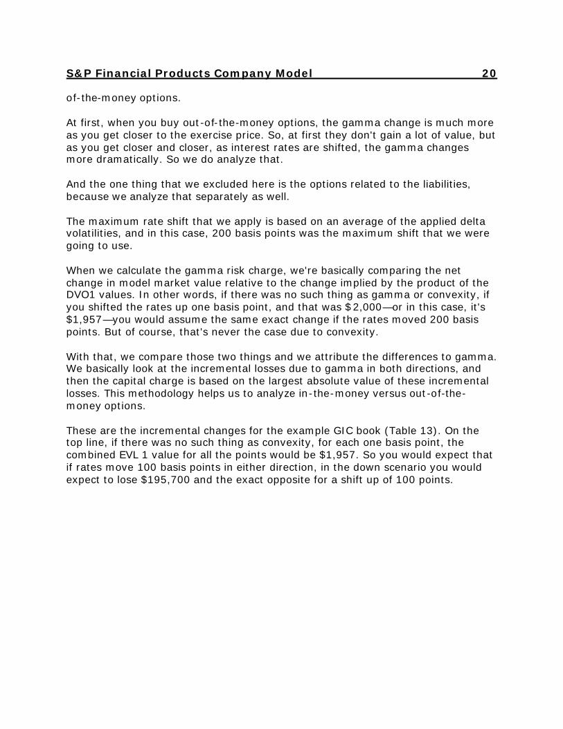
S&P Financial Products Company Model 20 of-the-money options. At first, when you buy out-of-the-money options, the gamma change is much more as you get closer to the exercise price. So, at first they don't gain a lot of value, but as you get closer and closer, as interest rates are shifted, the gamma changes more dramatically. So we do analyze that. And the one thing that we excluded here is the options related to the liabilities, because we analyze that separately as well. The maximum rate shift that we apply is based on an average of the applied delta volatilities, and in this case, 200 basis points was the maximum shift that we were going to use. When we calculate the gamma risk charge, we're basically comparing the net change in model market value relative to the change implied by the product of the DVO1 values. In other words, if there was no such thing as gamma or convexity, if you shifted the rates up one basis point, and that was $2,000—or in this case, it's $1,957—you would assume the same exact change if the rates moved 200 basis points. But of course, that's never the case due to convexity. With that, we compare those two things and we attribute the differences to gamma. We basically look at the incremental losses due to gamma in both directions, and then the capital charge is based on the largest absolute value of these incremental losses. This methodology helps us to analyze in-the-money versus out-of-the-money options. These are the incremental changes for the example GIC book (Table 13). On the top line, if there was no such thing as convexity, for each one basis point, the combined EVL 1 value for all the points would be $1,957. So you would expect that if rates move 100 basis points in either direction, in the down scenario you would expect to lose $195,700 and the exact opposite for a shift up of 100 points.


Table 13

35Page


• MR2 “Gamma” risk charge = $5,868,121 or 0.587% of GICs


Calculating MR2“Gamma” Risk Charge

-200 -150 -100 100 150 200

Expected incremental change in market value * (97,850) (97,850) (195,700) 195,700 97,850 97,850

Modeled incremental change in market value 3,851,728 (485,178) (2,984,232) (5,672,421) 3,035,440 3,862,751

Unexpected gain or loss related to gamma 3,949,578 (387,328) (2,788,532) (5,868,121) 2,937,590 3,764,901Summation of losses in directional scenario

Total MR-2 Incremental Capital Charge:*Note: Based on DV01 value of 1,957 for 1 basis point upward parallel shift.

(3,175,859) (5,868,121)

5,868,121

Simulated Downward Shifts Simulated Upward ShiftsMarket Value Change In Portfolio ($)

Table showing “Gamma” calculations

The next two shifts are a little confusing. But the next two shifts are for the change for an additional 50 basis points. On the next line, we look at the incremental change based on the model values that were provided previously. You can see that this has a huge change here, and that's because those options, the swaptions, go way into the money at that point and change quite dramatically. So the next step for us then is to compare the expected change versus the actual change. In other words, if you look at the first point there, we would expect a loss of $195,700; but what we actually got was a loss of $2.9 million. So the amount that we would attribute to gamma there, or negative convexity, is $2.7 million. So we do that in both directions, add up only the losses, and then take the worst-case loss. In this case, it's $5.8 million, or 58 basis points relative to the GIC book, and that becomes the gamma charge. We look at it incrementally because, if we didn't do that, we'd say, "OK, they're good. Everything is good, because when they got that 200-basis-point shift, everything looked good." So that's why we look at the incremental shifts instead, because when people buy out-of-the-money options, they're fairly cheap, but they may or may not provide protection over the non-tailed events.

S&P Financial Products Company Model 22 FROM THE FLOOR: How did you get that $3.1 million? MR. ROSEMAN: Well that's supposed to be the addition of $387,328 and $2,788,532. FROM THE FLOOR: Oh, you summed that? MR. ROSEMAN: Yes, I summed the incremental losses. I forget about the gains; I just look at the losses. In the down scenario, we're saying, "Well, geez, what if rates only went down 150?" Then this becomes much more of a tail event as you get out here. In situations in which people are really long, in-the-money options, you could have positive gamma in both directions. In that case, we'll apply that positive gamma against your delta exposure. There's nothing wrong with that, to buy options to get rid of some of your mismatched exposure. So we'll reflect that here. FROM THE FLOOR: What bothers me is that you have 100 basis points down to 150. It's not that much independent. I mean, you're adding two things that get all the way down to 150 basis points. Why are you not getting the maximum? MR. ROSEMAN: Well, if it went down 150, it would be $3.1 million. If you only went 100, then it would be $2.7 million. FROM THE FLOOR: Is this table showing the incremental amounts? MR. ROSEMAN: It's incremental, yes; and that's confusing. FROM THE FLOOR: Then you have to change that. MR. ROSEMAN: Yes I should change that, because I thought that was confusing, too. Calculating Risk Charges for Liabilities When we calculate the option risk charge for liabilities, the first thing that we do is calculate assumed benefit withdrawal assumptions. And the companies provide us with a benefit withdrawal history, and then we determine a weighted average and the standard deviations of withdrawals. Then the withdrawal assumption that we use is the greater of five percent or the average plus, in this case, 2.5 standard deviations. And for the illustrated book here, we basically used a five percent assumed withdrawal rate. Then we quantify the losses given the assumed benefit withdrawal assumption and

S&P Financial Products Company Model 23 applied series of adverse rate movements. In this case, the final shift that we apply is 200 basis points, which is the same as the gamma shift. The companies provide us with the market and book values for the GIC, as well as the value of the hedges given the specified upward rate movements. Originally, we were just going to take something based on their modified duration. Say, if rates go up 200 basis points, we're going to nail them for the change in market versus book that's implied by that change. But if you have a situation where a company is writing GICs and rates have gone down 200 basis points, then even if rates go up 200 basis points and all the cash is drawn out to benefit responsive activity, it's a neutral event for the companies since there is no cost on the benefit responsive event since book value is equal to market value.. The flip side of that is if rates go up 100 basis points, and then we're testing up another 200, that's a definite bad event. So this part of the model covers both sides of that. In the example portfolio, the charge we came up with was 38 basis points, or $3.8 million, which would be fairly typical. Credit Risk The next thing I'm going to talk about now is how we calculate the capital adequacy for credit risk. We have the actual credit default factors that we apply to the credit exposures (Table 14). This is for an AA-rated company; it would be different if it was a single–A- or BBB-rated company or an AAA-rated company.

Table 14

Year: 1 2 3 4 5 6 7 8 9 10 AAA Default Factors 0.015% 0.023% 0.039% 0.080% 0.124% 0.258% 0.405% 0.682% 0.812% 0.974%

1 std. Deviation 0.009% 0.017% 0.028% 0.058% 0.087% 0.096% 0.116% 0.170% 0.213% 0.308%2.57 Std. Deviations 0.023% 0.044% 0.072% 0.149% 0.223% 0.247% 0.299% 0.437% 0.548% 0.792%

Total AAA gross factors 0.038% 0.067% 0.111% 0.229% 0.347% 0.504% 0.704% 1.120% 1.361% 1.766% AA Default Factors 0.051% 0.087% 0.122% 0.253% 0.411% 0.611% 0.787% 0.933% 1.019% 1.107%


Total AA gross factors 0.079% 0.241% 0.276% 0.585% 0.911% 1.341% 1.652% 1.903% 2.032% 2.172% A Default Factors 0.057% 0.154% 0.253% 0.411% 0.610% 0.791% 1.036% 1.192% 1.423% 1.681%


Total A gross factors 0.097% 0.279% 0.428% 0.699% 1.067% 1.383% 1.740% 2.010% 2.402% 2.896% BBB Default Factors 0.232% 0.538% 0.820% 1.329% 1.767% 2.217% 2.615% 2.988% 3.311% 3.594%


Total BBB gross factors 0.456% 1.024% 1.504% 2.193% 2.777% 3.358% 3.866% 4.490% 5.131% 5.664%

Standard & Poor's Default Study for a "AA"-rated companyDiscounted Cumulative Default Factors With Discounted Standard Deviation Movements

S&P Financial Products Company Model 24 We would start with the historical default factor, and we discounted that. That .122 reflects the discounting. We then looked at a standard deviation. Every year Standard & Poor's calculates those default studies, by creating a pool of assets, and they track those pools throughout their life and see how many defaults they have based on rating. In the first year they started this, let's say they were looking at how many single-As defaulted after year one. This is totally unrealistic, but I'll just pull numbers our to the air: Say they say at two percent default; so they put that and they publish, "OK, we have two percent default for single-As in year one." Then they keep track of that one. Then when the next one comes through, let's say that has four percent defaults for single-As in year one. Take those together—you've got two percent and four percent—and they say it's three percent. They publish that, and they keep doing that. It's not exactly how it works, but it's a simplified method; so the default factors that Standard & Poor's publish will reflect sort of an average. So we're taking a standard deviation of those data fields. FROM THE FLOOR: What rate do you use? MR. ROSEMAN: To discount them? FROM THE FLOOR: Yes. MR. ROSEMAN: It's not very scientific, but I propose that we discount it along the yield curve. Actually, I'm not using the cumulative default rates; I'm using incremental default rates, discounting those back along the yield curve at the given point for the incremental, and then summing them back together. We do that because if you have situations where somebody stays long, like a 10-year security, and buys a credit derivative in which they're taking out the back five years of that, you can't just use a cumulative default. You have to use incremental defaults for each of those years along there. So that's how we do it, but I don't want to torture everybody else. FROM THE FLOOR: What do you use in practice? MR. ROSEMAN: I'm sorry—I didn't finish explaining this, actually. If an AA company was holding an AA-rated security, the factor that we would use is at this point would be 27. Where that comes from is, historically, for a three-year maturity, this is discounted. I don't know what the raw number was. But after the discounting, we would assume that .122 percent of AA securities default in year three. Now some of this has been massaged.

S&P Financial Products Company Model 25 FROM THE FLOOR: Is the rating the rating at time of purchase or the current rating? MR. ROSEMAN: We just do it based on whatever it's rated right now. It's AA at issue. They don't really look at trend; they do look at that, but this doesn't really reflect transitional default. It's like AA when it first came into these pools I was talking about. FROM THE FLOOR: Shouldn't they look at the rating at issue too? MR. ROSEMAN: They take these pools, and it's all the AAs that started out. They calculate what percentage defaults in each year, and then they average them together. I mean, we do offer data on transitional downgrades and so forth. FROM THE FLOOR: We don't know whether it's AA at issue or AA at the time that you calculated it. You've been jumping back and forth. MR. ROSEMAN: When we apply this model, I don't care where it's been or where it's going; I'm just looking at what it is now and what could possibly be the outcome. Does that make sense? In other words, I'm looking at your portfolio, how it's rated right now. If you have an AA security right now, there's no chart that says or no study that looks at AAAs that were downgraded to AA. If you have an AA security right now, that rule of finance is, you know you don't want to look at the past and decide what you're going to do in the future. If you have an AA-rated security right now, and you're looking out three years, that's the probability of default in that security. It's irrelevant as to how it got to be AA. I agree that maybe there is some statistical analysis that could be done. I would venture to say that things that have gotten downgraded over the first three years, maybe there's a higher probability that they're going to default. But we don't have that type of resolution in our data, if that's what you're implying. This is the breakdown for the fixed income securities and creditor evidence, when we apply the default factors (Table 15). If something is an amortizing asset, we basically use the average life. This is typically how companies give us that data.


Table 15

39Page


Step 2: • Company provides par value of fixed-income securities & credit

derivatives categorized by rating and term to maturity– Average life used for amortizing securities

Analyzing R2 - Credit Risk

Calculating CR1 Non-Financial Market Credit Risk Charge

Maturity Range AAA AA+ A+ A- BBB+<1 yr 50,000

1 to 2 yr2+ to 3 yr 118,750 118,750 3+ to 4 yr 118,750 118,750 4+ to 5 yr5+ to 6 yr 25,000 118,750 6+ to 7 yr7+ to 8 yr8+ to 9 yr

9+ to 10 yr 50,000

CR1 - Credit Exposures ($000's)Rating Category

So then we basically calculate the expected credit losses on the fixed-income securities, netted the salvage by multiplying the gross default factors by the par amounts and then we applied a 45 percent salvage value. There's no credit risk charge for U.S. government-issued securities or government-sponsored enterprises. For expected credit losses on short credit derivatives, this is determined using the same calculations. If you look at General Mills, we round it up to two years; it's 1.9 years to maturity (Table 16). It's at $118 million par, the factor was .277 percent (28 basis points). Multiply those together, you get a salvage credit of 45 percent, and the capital charge related to that is $182,000.


Table 16

41Page

Illustrative applicationAnalyzing R2 - Credit Risk

Calculating CR1 Non-Financial Market Risk Charge

<table showing CR-1 calculations>

Step 3: (Calculations)

S&P Par Applied Gross CR-1 Salvage Net CR-1

Issuer / Description Rating Date Years Amount Factors Charges Credit ChargesNational Rural Utilities A + 1/15/2002 0.18 50,000,000 0.10% 48,452 45% 26,649 General Mills A- 10/8/2003 1.91 118,750,000 0.28% 331,313 45% 182,222 Aon Corp A + 7/1/2004 2.64 118,750,000 0.43% 508,131 45% 279,472 Ford Motor Credit BBB+ 1/13/2005 3.18 118,750,000 0.04%* 45,695 45% 25,132 Bank of America A + 10/15/2006 4.93 118,750,000 1.07% 1,267,063 45% 696,884 Paine Webber Group AA+ 5/16/2011 9.52 50,000,000 2.17% 1,085,972 45% 597,285 Money Store - Home Equity AAA 8/15/2039 5.12 25,000,000 0.50% 126,068 45% 69,337 Fannie Mae - CMO-PAC AAA 7/25/2027 25.71 200,000,000 N/A - - -Ginnie Mae - Pass-Through AAA 4/15/2030 28.43 200,000,000 N/A - - -"Short" Sears Roebuck - Credit DerivA- 1/18/2005 3.19 118,750,000 0.70% 830,432 0% 830,432

Totals: 1,118,750,000 2,707,414

Maturity

CR1 - Fixed Incom & Credit Derivative - Calculations

• CR1 Credit risk charge = $2,707,414 or 0.271% of GICs

* Reflects joint prob. of default on Ford Motor Credit & counterparty credit default swap

We then add them all up, and for this book, the CR 1 capital charge for the fixed income securities and credit derivatives was $2.7 million. And you can see the Sears Roebuck, we assume that they wrote a credit derivative there. It's got the same exact capital charge as if you had 3.19-year bond, basically. If you look at the Ford Motor Credit, that basically reflects the joint probability of our default factor for Ford Motor Credit being, it's BBB, and the AA counterparty we assume that they bought it from. So the credit charge is $2.7 million, or about 27 basis points relative to the size of the GIC book. The next thing we do is we calculate the counterparty credit exposure. Then we used the same methodology that we used for the fixed-income securities and calculated the expected losses. In this case, it works out to be about two basis points, or $176,000. The last thing we do is calculate an operational risk charge. In the case of the hypothetical GIC book here, it came out to be 32 basis points or $3.2 million. We applied a 30-basis-point charge to their benefit-responsive GIC liabilities and 1 basis point to the OTC derivatives. It didn't come out to be 31 basis points is because the notional amount of the derivatives is more than the notional amount of the GIC liabilities.

S&P Financial Products Company Model 28 In total, It worked out to be about 168 basis points for their financial market risk and 29 basis points for credit risk. We assume that there was no concentration risk. For the operating risk, it was 33 basis points for a total of 230 basis points. This model has no multiplier, but if that were an AA company, that's the amount of capital that we would expect to be held against the business. Now, I'm going to compare this to our traditional RBC model. The traditional model is a factor-based model; the FPC model is based on your actual exposure. People are going to argue, but I always say that with the FPC model, if you don't like that capital charge, then you're basically saying you don't like your exposure. That's not 100 percent true, but to some degree it might be. In the traditional model, the analysis is based on average industry risk. In the FPC model, it's based on your company-specific risk. In the traditional model for Standard & Poor's, the capital adequacy for credit risk is based on four factors using NAIC code. For the FPC model, the capital adequacy for credit risk is based on our corporate default studies. The traditional model doesn't and can't consider hedging strategies. In the FPC model, we consider all sources of credit and market exposure, regardless of what the source is. And last, for the traditional model, it's a broadly applicable model. The FPC model has limited applications, and companies have to basically tell us that they want to have it applied, and we offer that as a service. The last thing we did was a comparison of doing that same hypothetical GIC book using our traditional model and our FPC model, and it's a pretty large difference. In the traditional model, you have 5.49 percent capital adequacy expected by Standard & Poor's; and using the FPC model its 2.3 percent. To be honest, a lot of it on the RBC model is assumed. We didn't go through and do the MBS calculations. So we assume that we use a 4 percent default for the additional convexity charge. But in any case, the data is fairly compelling. Just as a wrap-up, you know the FPC model is a sophisticated tool in Standard & Poor's now. It applies to insurance companies. The model affords Standard & Poor's a much greater resolution than our traditional model. That allows us to feel comfortable, even if the amount of capital is a lower amount of capital, it's the correct amount of capital. And last, we think that the model can add a lot of value to insurance companies seeking to optimize their capital reserves. MS. ELLEN WOODRUFF HALL: Today I will be discussing the management of interest rate risk at ING Institutional Markets and the implementation of the FPC

S&P Financial Products Company Model 29 capital model. Specifically, I will be focusing on the delta and gamma market risk charge. By walking through two examples of hedging away both delta and gamma risks, we will see how you can use the FPC model to effectively minimize risk. At year-end 2001, ING Institutional Markets was an $8.4 billion GIC business, predominantly consisting of stable value GICs and funding agreements on the liability side; and bonds, CMOs, and commercial mortgages on the asset side. What Does ING Do? Since the objective of the institutional markets business unit is to maximize the risk-adjusted return on capital (RAROC), it is necessary to understand all pertinent risks facing the business unit, including interest rate risk, credit risk, liquidity and operational risk. Today I will be specifically looking at managing interest rate risks. I will first walk through the interest rate risk management process at ING Institutional Markets. Each week ING Institutional Markets evaluates the interest rate risk it is exposed to. The risk is measured as the market values change under parallel shocks, ranging from 10 to 300 basis points to the yield curve, as well as shocks to 10 key rate points along the yield curve. ING Institutional Markets use key rate duration as a critical tool in managing interest rate risk. Managing key rate duration minimizes adverse market value changes when interest rates move in a nonparallel shift, thus changing the shape of the yield curve. Furthermore, ING Institutional Markets minimizes interest rate risk by swapping fixed-rate assets and liabilities to one- or three-month LIBOR. The tools in place to measure our interest rate risk are modeling systems, and we are using quantitative risk management (QRM). The QRM modeling system calculates the market value under the current yield curve, as well as your market value change under key-rates and parallel shocks. QRM also calculates projected income under various scenarios. QRM originated many years ago as a banking asset/liability (A/L) system. We also use the Intex database to obtain collateral information necessary to model our collateralized mortgage obligations and also asset-backed securities. The Bloomberg system and the ING Investment Management Group provide institutional markets with the information necessary to model our assets and derivative trades each week. Before implementing the FPC model, a company needs to demonstrate to S&P that it is regularly monitoring and effectively managing risk.

S&P Financial Products Company Model 30 Before institutional markets began looking into the FPC model, we developed a weekly process to manage interest rate risk by incorporating both key rate and parallel duration into our analysis. As I mentioned, we model our new trades each week as well as the entire in-force block on an ALM system—in our case, QRM. Impact on Key Rates We then evaluate the impact of changes in interest rates on key rate market value sensitivities, broken down by asset, liability and derivative type. In addition to key rate duration, we calculate parallel duration under 12 shocks, ranging from 10 to 300 basis points up and down. We also calculate the FPC delta and gamma capital charge each week. Our energies are really focused on our weekly risk management. However, at the end of the month, we need to reconcile our weekly trades and models in force to the actual holdings provided to us on the accounting files. In addition, on a monthly basis, we track and compare actual investment income to model income to ensure that the modeling of the assets, derivatives and liabilities is correct. Moving on to our quarterly risk management process, we really focus on the ALM reporting for the North American ING group, while providing information under 100 ALM scenarios. The second piece of our quarterly risk management is to provide to the S&P group the necessary information for them to calculate our capital under the FPC model. Managing Market Risk Using the FPC model Now we'll switch gears from how ING Institutional Markets manages interest rate risks to how you can use the FPC capital model to manage market risks within your company. As Bob Roseman pointed out earlier, there are three components of market risk under the FPC model. The first component is delta risk, which is your market value change under key rate points along the yield code. The second component is gamma risk, the market value change under various parallel shocks, ranging from one basis point to 250. And the third component is the option risk embedded into liabilities, such as the benefit responsiveness on pension plans. Today I will focus on how to hedge away delta and gamma risk. Now we will walk through an example to demonstrate how managing key rate duration can prevent adverse market value changes when the shape of the yield curve changes, such as the curve steepening all of us experienced during 2001 (Table 17).


Table 17

11

Why Manage Interest Rate Risk Along Key Rate Points?

Ø Example: • 12/31/2000 interest rates• 10 year amortizing bond with duration = 4.4 years• Swap fixed rate bond to floating rate to match durations

– Hedge parallel duration or key rate duration?– Non-Amortizing Swap with Maturity of 5.2 years– Amortizing Swap with Maturity of 10 Years

• MR-1 capital (based on year-end 2000 rates)– Bond + Non-Amortizing 5.2 Year Swap

– Delta Capital =1.73%– Duration matched under parallel shocks, yet significant curve risk

– Bond + Amortizing 10 year Swap – Delta Capital = 0.20%– Mitigated interest rate curve risk, as well as interest rate risk under

parallel shocks

The simple example that I will be walking through is how to swap a fixed–rate, 10-year amortizing bond to floating rate to obtain a duration mismatch of zero. The duration of the bond valued under the swap curve is 4.4 years. Now, keep in mind that this an amortizing bond. If we were only managing duration under parallel shocks to the yield curve, we could enter into a nonamortizing swap with a maturity of 5.2 years, which has a duration of 4.4 years matching the bond. So when you look at the interest rate of the bond and the swap together, your net duration would be zero—there's no exposure to changes in interest rates. However, this trade results in significant risk along the yield curve (Table 18). Here are market value changes to the various key rates. In this example, we have 10 key rates ranging from the one–month to the 30-year. And our key rate shock is an up 10 basis point shock. So the first column illustrates your key rate duration on the bond, a 10-year amortizing bond.


Table 18

12

QRM Market Value Shocks Report “Market Value Change”

Bond Bullet Amortizing Bond+ Bond +Amortizing Swap Swap 5.25 Yr Amort

SUBACCOUNT 10 YEAR 5.25 Year 10 Year Swap 10 Yr Swap

Face Amount 100,000,000 (100,000,000) (100,000,000) Market Value 100,000,000 - - MVC - DOWN 10 444,000 (440,000) (435,000) 4,000 9,000 MVC - UP 10 (440,000) 437,000 432,000 (3,000) (8,000)

MVC - KRD-1 - (5,000) (8,000) (5,000) (8,000) MVC - KRD-3 - (11,000) - (11,000) - MVC - KRD-6 (1,000) 1,000 1,000 - - MVC - KRD-12 (13,000) 5,000 14,000 (8,000) 1,000 MVC - KRD-24 (25,000) 10,000 26,000 (15,000) 1,000 MVC - KRD-36 (58,000) 24,000 57,000 (34,000) (1,000) MVC - KRD-60 (96,000) 348,000 96,000 252,000 - MVC - KRD-84 (136,000) 65,000 136,000 (71,000) - MVC - KRD-120 (111,000) - 110,000 (111,000) (1,000) MVC - KRD-360 - - - - -

Total Key Rate MVC (440,000) 437,000 432,000 (3,000) (8,000) Duration 4.4 0.0 0.1 MR-1 "Delta" Capital 1,730,500$ 200,593$

The second column looks at the duration of a 5.2-year swap, nonamortizing. And the third column is the market value sensitivity on an amortizing 10-year swap. If we put the bond with a 5.2-year bullet swap, you see significant risks along the five-year point—we're actually short duration at the five-year point because of the swap. And yet we're exposed to significant long duration—at the five- to 10-year point because of the cash flows on the bond. Now, if we look at the sensitivity of the bond plus the amortizing swap, the very bottom line overall, you have a duration of zero—or actually in this case, 0.1. It's very similar to the overall duration of the bond, plus the 5.2-year duration match swap. However, notice on the bond plus amortizing swap, you have very little risk along the key rate points, unlike if you were swapping the amortizing bond with the 5.2-year swap. How does this translate into delta capital? The very bottom line on this trade, the bond plus the nonamortizing swap, you would hold $1.7 million in capital. And this is based on a $100 million national bond, versus having that same bond with an amortizing swap result in $200,000 in capital. So by using an amortizing swap, you are reducing your delta capital by a percent and a half. Let's look at the market value of the bond and swap one year later:

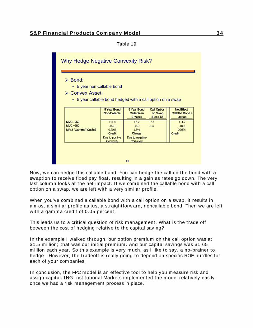
S&P Financial Products Company Model 33 The trade I modeled was put on the books December 31, 2000. Now we've valued this transaction one year later at year-end 2001, after we've experienced significant curve steepening. The market value of the bond actually increased $3.6 million; however the market value on our nonamortizing swap decreased $4.5 million, even though at the onset of the trade our overall duration mismatch was zero. Yet, we were seeing significant long and short duration along the yield curve. So as that yield curve steepened, we're left with almost a $1 million dollar loss. If we had entered into a 10-year amortizing swap to match the bond cash flows, our net loss on the bond plus swap would have been zero. You'll see the decrease in the market value on the amortizing swap was also $3.6 million to match the increase on the bond. So, not only were we able to hold less delta capital, a year later if you marked your books to market by using an amortizing swap, you would have seen no loss. This next example illustrates why a company should hedge negative convexity risk. We look at the market value change under parallel shocks to the yield curve. A bond with no optionality, a very straightforward, five-year, non-callable bond exhibits positive convexity. I think most of us are familiar with that. You're going to make more money as rates go down than you lose as rates go up. Now, under the FPC model, because we exhibit positive convexity on this bond, we'll actually receive a credit to our gamma capital, which, as Bob pointed out, would then be applied to our delta charge. Convexity I've modeled a simple, five-year bond with a call in two years to illustrate negative convexity (Table 19). And here you're going to lose more money when rates go up than the amount of money you would make when rates went down. Because of the negative convexity in this callable bond, you actually receive a gamma charge of 1.6 percent.


Table 19

14

Why Hedge Negative Convexity Risk?

Ø Bond:• 5 year non-callable bond

Ø Convex Asset:• 5 year callable bond hedged with a call option on a swap

5 Year Bond 5 Year Bond Call Option Net Effect Non-Callable Callable in on Swap Callalbe Bond +

2 Years (Rec Fix) Option

MVC - 250 +11.4 +6.2 +5.5 +11.7MVC +250 -10.0 -8.9 -1.4 -10.3MR-2 "Gamma" Capital 0.20% 1.6% 0.05%

Credit Charge CreditDue to positive Due to negative

Convexity Convexity

Now, we can hedge this callable bond. You can hedge the call on the bond with a swaption to receive fixed pay float, resulting in a gain as rates go down. The very last column looks at the net impact. If we combined the callable bond with a call option on a swap, we are left with a very similar profile. When you've combined a callable bond with a call option on a swap, it results in almost a similar profile as just a straightforward, noncallable bond. Then we are left with a gamma credit of 0.05 percent. This leads us to a critical question of risk management. What is the trade off between the cost of hedging relative to the capital saving? In the example I walked through, our option premium on the call option was at $1.5 million; that was our initial premium. And our capital savings was $1.65 million each year. So this example is very much, as I like to say, a no-brainer to hedge. However, the tradeoff is really going to depend on specific ROE hurdles for each of your companies. In conclusion, the FPC model is an effective tool to help you measure risk and assign capital. ING Institutional Markets implemented the model relatively easily once we had a risk management process in place.

S&P Financial Products Company Model 35 MR. FOWLER: Thanks Ellen and Bob. FROM THE FLOOR: I have two questions; the first one is for Bob. I didn't understand about how to cover salvage value. Do you use just the average observed…? MR. ROSEMAN: The salvage value? FROM THE FLOOR: Yes, the industry experience or do you take into account a company specific experience? MR. ROSEMAN: Basically, we look at the industry. We have studies in Standard & Poor's—we do the salvage value; we basically take the average. FROM THE FLOOR: So, you take no company experience? MR. ROSEMAN: No, but that's not to say you wouldn't potentially do that. As I mentioned, earlier, we're definitely willing to run that up the flagpole at a committee. So if you have particularly good experience in that regard, it's something we would definitely consider. FROM THE FLOOR: OK. Another thing, I'm working for Aegon Institutional Markets, so I'm interested in Ellen's presentation. I have a couple of questions related to your presentation. The first one is, I know for most institutional markets we run floating business for ALM purposes, but I don't quite understand the reason you have to run a risk profile—a management profile—on a weekly basis. Because if you want a full float block of business, the interest rate changes in a week are relatively small. Then another question I have is, based on experience, I think the biggest advantage is that you can manage your risk better. You also can reduce the capital charges. But are there any other findings from your experience that you did not anticipate and just have discovered after you implemented this new process? MS. WOODRUFF HALL: To address your first question, why do we look at our risk management, specifically our interest rate risk weekly? We want to ensure that any trades that went on the books during the week were effectively hedged. And the second part is, we're providing to S&P our information quarterly for our quarterly calculation of capital. When you're managing interest rate risk, you don't want any surprises after the close of the quarter. By monitoring this weekly and really seeing the market value changes as interest rates move each week, we're able to track that. And as we all know, there are many surprises in interest rates—the end of 2000 and into 2001, for example. At the onset of the trade, you believe you're effectively hedged; but as

S&P Financial Products Company Model 36 the curve twists and turns, those hedges you put on are not always 100 percent effective. So you can really get at that weekly. FROM THE FLOOR: Are there any other findings from your experience that you did not anticipate and just have discovered after you implemented this new process? MS. WOODRUFF HALL: To be honest, there really was not. But part of that was, we did not just one day say, "Bob we want to implement the FPC model." It took us two to three years to really develop a solid risk management process. We moved from a traditional insurance system, such as TAS or PTS and many of the others to more of a banking, ALM system in QRM. FROM THE FLOOR: One of the things I wasn't sure if I caught, if it was inherently in the model and I missed it or if it's not there, was the effect of credit risk changes, credit risk spreads changing in the model. How that is actually captured, or is it inherently outside of the model? MR. ROSEMAN: That's actually a good question; it means you were paying attention. That's actually not covered in the model. We feel our interest rate volatilities are large enough that it overstates the capital we need for the absolute rate shifts. However, that aside, I'm looking at a company right now that's come to us and one of their strategies is to synthetically cash match their book, but they buy much longer average life assets versus their liabilities. So at that point, you have a lot of spread duration risk. If the spread widens out to LIBOR, you have risks. So we're going to do the same type of methodology in which we're going to do statistical analysis and look at spread widening and apply that. I hope that answers your question. FROM THE FLOOR: Are you looking to pay more attention to spread duration risk in the future? MR. ROSEMAN: Yes. FROM THE FLOOR: And right now, it's regularly covered by the conservatism? MR. ROSEMAN: We also make an assumption that most of the companies aren't that mismatched in terms of spread duration risk. So I don't think it's that important a component of risk for most companies. And if somebody is specifically drawing our attention to that, or we see a situation where, say if somebody starting buying or writing credit spread derivatives with very different average lives, then we're definitely concerned with that. MR. MICHAEL KAUFMAN: This question is for Bob. As I understand the FPC

S&P Financial Products Company Model 37 model, the credit risk piece is at least conceptually analogous to C1, market risk to C3, and operational risk to C4. MR. ROSEMAN: Right. MR. KAUFMAN: In the FPC model, I don't recall any sort of a covariance term between the three pieces. Can you comment on that? MR. ROSEMAN: Actually there is none. That's something that we've been approached on, but to date we haven't really addressed that. So you're basically saying, "If you're reserving for those three things, the probability of getting whacked on all three at the same time is not that great." But I haven't reflected that in yet. But stay tuned. MR. LARRY GORSKI: The question is probably for both of the speakers. What do you see as the implications for the insurance industry of, let's say, the S&P model that's more customized, company-specific, capital-adequacy-type model, versus the regulatory framework, which is still based on an industry average approach? How do you see that this continuity and approach is affecting the insurance industry? MR. ROSEMAN: I think you're going to have a situation in which either one of those two factors is going be the limiting factor of how much capital... If we come up with a model that requires less capital than the NAIC, then it basically doesn't provide the company value, because that's what they have to capitalize to. I hope that answers your question. MR. GORSKI: Well, I guess my question is probably a little deeper than that. I was trying to determine whether there would be a greater push from the industry to pressure regulators to develop a more company-specific type model as opposed to an industry-average type model. That's what I was really getting at. MR. ROSEMAN: OK, I think there actually might be some precedent for that in the BIS capital model as applied to banks. The FPC model is similar to that; it's probably more detailed than the original BIS capital model. But now the bank regulator is now moving toward letting companies use their own VAR models and so forth. So with all this risk management stuff, I think that the banks have sort of set the stage, and insurance companies have kind of been second in the door. So maybe that will be the case. It's not my area of expertise.


Chart 1

23Page

Corporates57%

MBS (Pass-thru)

20%

MBS (CMO-PAC )20%

ABS (HEL)

3%

$1 billion Assets by Sector Type

Illustrative applicationSelect Characteristics of Hypothetical “GIC” Book

$1 billion Assets by Rating

A+29% AA+

5%

AAA42%

BBB+12%

A-12%

Average rating = “AA-” (GSE’s = 40%)

Chart 2

24Page

Illustrative applicationSelect Characteristics of Hypothetical “GIC” Book

$60 million OTC derivative counterparty exposure by rating

A31%

AA42%

AAA27%

$1 billion benefit responsive GICs

4 yr35%

2 yr10%

3 yr35%

1 yr5%5 yr

10%

7 yr5%

Documents

RECORD, Volume 28, No. 1* - Society of Actuaries