Embed Size (px)
Citation preview
Near Surface Geophysics, 2017, 15, 187-199 doi: 10.3997/1873-0604.2016050
187© 2017 Authors. Near Surface Geophysics is published by European Association of Geoscientists & Engineers This is a Gold Open Access article under the terms of the Creative Commons Attribution License, which permits use, distribution and reproduction in any medium, provided the original work is properly cited.
Reconstruction quality of SIP parameters in multi-frequency complex resistivity imaging
Maximilian Weigand1*, Adrián Flores Orozco2 and Andreas Kemna1
1Department of Geophysics, University of Bonn, Meckenheimer Allee 176, 53115 Bonn, Germany2Institute of Geodesy and Geophysics, TU-Wien, Gusshausstrasse 27/29, 1040 Vienna, Austria
Received April 2016, revision accepted November 2016
ABSTRACTComplex resistivity imaging provides information on the subsurface distribution of the electrical conduction and polarisation properties. Spectral induced polarisation (SIP) refers to the frequency dependence of these complex resistivity values. Measured SIP signatures are commonly analysed by performing a Cole–Cole model fit or a Debye decomposition, yielding in particular chargeabil-ity and relaxation time values. Given the close relation of these parameters with petrophysical properties of relevance in various hydrogeological and environmental applications, it is crucial to understand how well they can be reconstructed from multi-frequency complex resistivity imaging with subsequent Cole–Cole or Debye decomposition analysis. In this work, we investigate, in a series of numerical simulations, the reconstruction behaviour of the main spectral induced polarisa-tion parameters across a two-dimensional complex resistivity imaging plane by considering a local anomalous polarisable body at different depths. The different anomaly positions correspond to dif-ferent cumulated sensitivity (coverage) values, which we find to be a simple and computationally inexpensive proxy for resolution. Our results show that, for single-frequency measurements, the reconstruction quality of resistivity and phase decreases strongly with decreasing cumulated sensi-tivity. A similar behaviour is found for the recovery of Cole–Cole and Debye decomposition charge-abilities from multi-frequency imaging results, while the reconstruction of the Cole–Cole exponent shows non-uniform dependence over the examined sensitivity range. In contrast, the Cole–Cole and Debye decomposition relaxation times are relatively well recovered over a broad sensitivity range. Our results suggest that a quantitative interpretation of petrophysical properties derived from Cole–Cole or Debye decomposition relaxation times is possible in an imaging framework, while any parameter estimate derived from Cole–Cole or Debye decomposition chargeabilities must be used with caution. These findings are of great importance for a successful quantitative application of spectral induced polarisation imaging for improved subsurface characterisation, which is of interest particularly in the fields of hydrogeophysics and biogeophysics.
Lesmes and Morgan 2001; Nordsiek and Weller 2008; Florsch, Revil and Camerlynck 2014; Weigand and Kemna 2016b).
While initially the IP method has been mainly used for the prospection of ore deposits (e.g., Pelton et al. 1978), over the last 15 years, the potential of CR imaging has also been demon-strated for various hydrogeological and environmental applica-tions, including lithological discrimination (e.g., Kemna, Binley and Slater 2004; Mwakanyamale et al. 2012), mapping and quantification of hydraulic conductivity (e.g., Kemna et al. 2004; Hördt et al. 2007), monitoring the integrity and performance of reactive barriers (Slater and Binley 2006), mapping and charac-terisation of contaminant plumes (e.g., Kemna et al. 2004; Flores Orozco et al. 2012a), monitoring of sulphide mineral precipita-tion (e.g., Williams et al. 2009; Flores Orozco, Williams and Kemna 2013), and monitoring of micro-particle injection and
INTRODUCTIONThe induced polarisation (IP) method yields images of the com-plex resistivity (CR) of the subsurface, which provides informa-tion on the conduction and polarisation properties of the meas-ured soils or rocks. The measurements can be performed at dif-ferent frequencies (typically below 10 kHz), in the so-called spectral IP (SIP) method, to obtain information on the frequency dependence of the CR.
Due to its simplicity, the Cole–Cole (CC) model is widely used to describe the SIP response (e.g., Pelton et al. 1978; Luo and Zhang 1998). Yet, in recent years, the Debye decomposition (DD) approach has been promoted as a robust and flexible alternative to the CC model in (near-surface) geophysical applications (e.g.,
M. Weigand, A. Flores Orozco and A. Kemna188
© 2017 European Association of Geoscientists & Engineers, Near Surface Geophysics, 2017, 15, 187-199
ed out for conventional resistivity imaging, it has not yet been addressed for single- or multi-frequency (spectral) IP imaging. The assessment of correlation loss is critical for the desired application of petrophysical models established on the basis of laboratory studies to imaging results obtained in the field.
We here investigate, by means of numerical simulations, the reconstruction quality of CC model and DD parameters recov-ered from multi-frequency CR images. We consider a standard dipole–dipole surface survey over a homogeneous, non-polarisa-ble half-space containing a 2D polarisable anomaly, whose verti-cal position is systematically varied to investigate its reconstruc-tion in areas with different sensitivity levels in the inversion. Hereafter, we refer to reconstruction quality as the deviation of the recovered model parameters from their original values. We analyse and compare the reconstruction quality of single- and multi-frequency (spectral) IP parameters as a function of cumu-lated sensitivity. We also investigate the impact of data noise on the reconstruction quality, considering that data quantification is critical for quantitative IP imaging applications (e.g., Flores Orozco, Kemna and Zimmermann 2012b; Kemna et al. 2012).
METHODSForward modelling and inversionSynthetic data, i.e., complex transfer impedances, are computed using the 2.5D finite-element modelling code CRMod (Kemna 2000). CRMod solves the underlying 2.5D forward problem (Helmholtz equation) for a given 2D CR distribution. For details of the implementation, we refer to Kemna (2000). Data noise is added from a normally distributed ensemble of random numbers. To provide comparable results, all simulations are conducted using the same ensemble of random numbers, scaled by previ-ously chosen standard deviations.
The noise-contaminated data are inverted using CRTomo (Kemna 2000), which is a smoothness-constraint, Gauss–
propagation (Flores Orozco et al. 2015). These field-scale appli-cations have also prompted the development of models describ-ing the link between the CR response and lithologic, textural, hydraulic, or geochemical soil/rock properties (see, e.g., Slater (2007), Kemna et al. (2012) and the references therein). The potential of the SIP method has also been demonstrated for applications in the emerging field of biogeophysics (e.g., Atekwana and Slater 2009). Examples of such applications include the detection of alterations at mineral–fluid interfaces due to microbial growth (e.g., Abdel Aal et al. 2004) or biostim-ulated mineral precipitation (e.g., Williams et al. 2009; Flores Orozco et al. 2011), detection of biofilm formation (e.g., Ntarlagiannis et al. 2005; Davis et al. 2006), and characterisation of tree roots (e.g., Zanetti et al. 2011) or crop roots (Weigand and Kemna 2016a). The variety of these studies demonstrates the growing interest in the application of CR (or SIP) imaging.
It is well known that electrical images are characterised by a spatially variable image resolution (e.g., Oldenburg and Li 1999; Friedel 2003; Binley and Kemna 2005), which needs to be taken into account in the interpretation of the resulting images. Day-Lewis, Singha and Binley (2005) found a spatially variable reconstruction quality of water content determined from electri-cal resistivity measurements, with an increasing inaccuracy of the inferred water content estimates with decreasing image reso-lution. This resolution-related phenomenon was referred to by the authors as “correlation loss”, as it can be considered as loss of information in the resistivity images due to poor resolution. Kemna (2000) demonstrated that the analysis of the cumulated sensitivity can provide insights into the variable image resolu-tion. Nguyen et al. (2009) found, for regions with cumulated sensitivity below some threshold value, an increase in the corre-lation loss for the mass fraction between fresh water and seawa-ter reconstructed from electrical resistivity imaging results. However, even if the problem of correlation loss has been point-
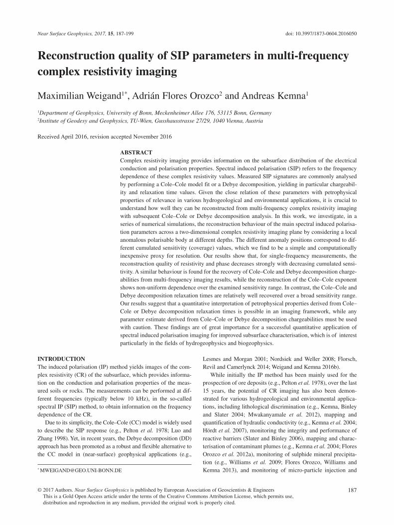
Figure 1 (a) Finite-element grid
used for the forward modelling.
(b) Distribution of percentage
errors of modelled impedance
magnitude values (ΔΖmod) for all
used measurement configura-
tions, determined for a homoge-
neous resistivity model (half-
space).
Reconstruction quality of SIP parameters 189
© 2017 European Association of Geoscientists & Engineers, Near Surface Geophysics, 2017, 15, 187-199
whereas τ values may span several orders of magnitude (e.g., Pelton et al. 1978; Vanhala 1997; Luo and Zhang 1998).
Debye decompositionThe DD scheme describes the CR spectrum using a superposi-tion of a large number of Debye polarisation terms (e.g., Nordsiek and Weller 2008):
(2)
where N is the number of relaxation times (i.e., Debye polarisa-tion terms) used for the superposition, m
k is the kth chargeability
corresponding to the kth relaxation time τk, and ρ0,DD is the DC
resistivity (as obtained from the DD). The relaxation times are chosen to cover the frequency range spanned by the data accord-ing to the inverse relationship τ = 1/ωmax, ρ'' (e.g., Weigand and Kemna 2016b). For each frequency decade, 20 relaxation times are used, and the relaxation time range is extended by two orders of magnitude at each end of the covered frequency range, as sug-gested by Weigand and Kemna (2016b,c).
The resulting distribution of relaxation times mk(τk) is called the relaxation time distribution, from which parameters similar to the CC parameters are derived:
• The total chargeability, , provides an analog to the CC chargeability m. However, mtot only accounts for polarisa-tion contributions within the data frequency range due to the much narrower spectral shape of the Debye response com-pared with typical CC responses (with c < 1).
• The mean logarithmic relaxation time, τmean, denotes the chargeability-weighted logarithmic mean value of the DD relaxation times (Nordsiek and Weller 2008):
DESIGN OF NUMERICAL EXPERIMENTSThe numerical experiments are conducted on a model domain of 80 m × 17 m (as depicted in Figure 1a), with the underlying finite-element mesh consisting of 3128 rectangular cells, each composed of four triangular elements. Forty electrodes are located at the surface with an equidistant spacing of 1 m. Only the quadratic finite-element cells below the electrodes are used for the analysis, and they are equally sized with an edge length of 0.5 m. To increase modelling accuracy, additional elements with an expo-nentially increasing width are used at both sides of the grid. Simulations are performed using a dipole–dipole measurement scheme composed of skip-0,1,2,3 configurations, resulting in 1944 measurements. The “skip-number” refers to the dipole length, indicating the number of electrodes “skipped” between the two current electrodes and the two voltage electrodes, respectively.
Newton-type inversion scheme. The data are weighted in the inversion by individual errors (see Appendix A).
Image appraisal is done using the L1- and L2-normed cumu-
lated sensitivity (coverage) and the diagonal entries of the model resolution matrix (see Appendix B). Throughout this study, nor-malised cumulative, error-weighted sensitivities (hereafter sim-ply referred to as sensitivity) are presented, as they offer better comparability.
Cole–Cole modelThe frequency-dependent electrical properties of soils and rocks are often described by the empirical CC model (e.g., Cole and Cole 1941). In terms of CR, ρ(ω), with angular frequency ω, the CC model can be expressed after Pelton et al. (1978) as
(1)
where ρ0 is the DC resistivity (low-frequency asymptote), m is the CC chargeability, τ is the CC relaxation time, c is the CC exponent, and j is the imaginary unit. Parameter ρ0 defines the amplitude of the magnitude spectrum (|(ρ(ω)|), whereas param-eter m determines the amplitude of the phase spectrum (φ(ω)). Parameter c describes the asymptotic slope of the symmetric phase spectrum (in log–log representation), i.e., the degree of frequency dispersion, and parameter τ is inversely related to the peak frequency of the imaginary part of the resistivity, i.e., ωmax, ρ'', by ωmax, ρ'' = 1/τ. The values of m and c range from 0 to 1,
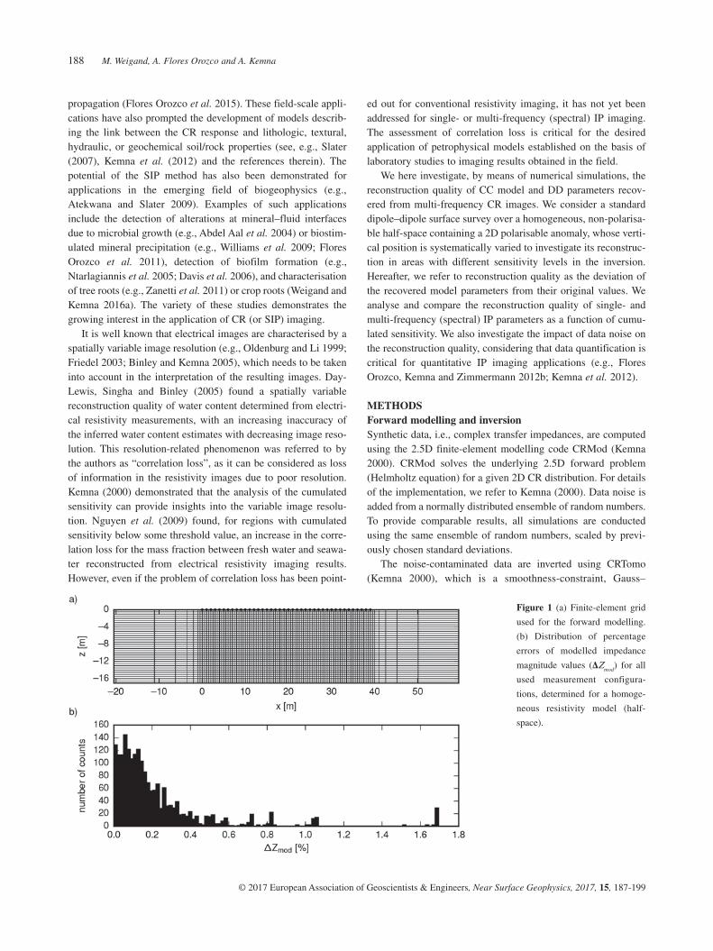
Figure 2 (a) Model used for the numerical simulations and (b) corre-
sponding (L2-normed) cumulated sensitivity distribution (normalised to
1). The model consists of a homogeneous half-space (|ρ| = 100 Ωm,
φ = 0 mrad) with an embedded polarisable anomaly (indicated by the
black rectangle), the depth position of which is varied in the simulations.
The positions of the surface electrodes are indicated by black dots. Outer
elements of the modelling grid are not shown (cf. Figure 1a).
M. Weigand, A. Flores Orozco and A. Kemna190
© 2017 European Association of Geoscientists & Engineers, Near Surface Geophysics, 2017, 15, 187-199
the polarisable anomaly. However, the diagonal entries of the model resolution matrix, i.e., (see Appendix B), are computed after the final iteration of the inversion process. As the final values of the regularisation parameter λ differ for the different anomaly locations, so do the computed diagonal entries of vary on this account (cf. equation (10)). Although this makes a quantitative comparison for the different anomaly locations difficult, the diago-nal entries of are presented in the following sections to show their general behaviour in comparison with cumulated sensitivity.
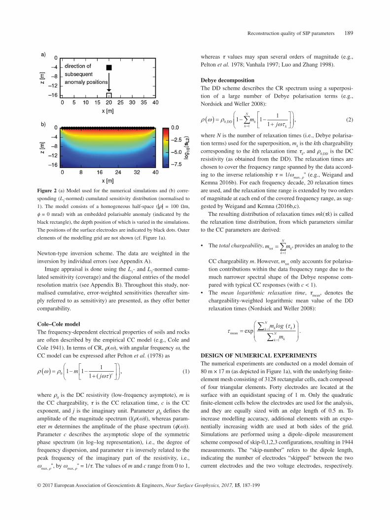
Single-frequency reconstructionIn a first step, we investigate the reconstruction quality of resis-tivity magnitude and phase values in the region of the anomaly, i.e., the deviation between original and recovered values, for a single-frequency data set. In the single-frequency studies, we investigate three scenarios: (i) 10 Ωm, –30 mrad (conductive, polarisable anomaly); (ii) 100 Ωm, –30 mrad (polarisable anom-aly); and (iii) 1000 Ωm, –30 mrad (resistive, polarisable anoma-ly). Figure 3 shows exemplary inversion results for the second scenario for two depths of the anomaly.
A small, stabilising noise component of 0.1% Gaussian noise is added to the impedance magnitude data, and Gaussian noise with a standard deviation of 0.5 mrad is added to the impedance phase data. The error estimate in the inversion assumes 3% rela-tive and 0.001 Ω absolute error for the impedance magnitude (resistance) and 1% relative and 0.5-mrad absolute error for the impedance phase.
The inverted resistivity magnitude and phase values of the anomaly pixels (i.e., model cells within the anomaly region) are averaged (arithmetic mean of log magnitude and phase, respec-tively), and the deviations from the original values are calculated as a measure of reconstruction quality. These deviations are analysed against the averaged (arithmetic mean of log values) cumulative sensitivity values (s
L1 and sL2), as well as against the diagonal entries of the model resolution matrix (diag( )), for the different anomaly locations.
Multi-frequency reconstructionThe next step in our study is to examine the reconstruction quality of the CC model parameters inferred from multi-frequency imag-ing results. The original CC parameters of the anomaly are chosen
For instance, the skip-0 configuration uses adjacent electrodes for current injection and voltage measurement. Resistance (imped-ance magnitude) modelling errors for a homogeneous half-space lie below 2% for all measurement configurations (Figure 1b).
The surface electrode configuration used in this study exhibits a cumulative sensitivity distribution that decreases monotonically with depth (Figure 2b). Thus, an anomaly placed at different depths in the subsurface (Figure 2a) is associated with different cumulative sensitivity levels. The CR model used to compute syn-thetic data is defined as a homogeneous background (|ρ| = 100 Ωm, φ = 0 mrad) containing an anomalous body (4 × 4 model cells, corresponding to a size of 2 m × 2 m) with varying resistivity magnitude and phase values. Since the spatial extension of the anomaly is relatively small (given the modelling domain and the used measurement configurations) and since anomalous resis-tivity magnitude values were only varied within one order of magnitude relative to the background value, the current density (and sensitivity) distributions do not differ significantly from the distribution for a homogeneous model. Therefore, we use the sen-sitivity values of the homogeneous model in the analysis of the reconstruction quality of the CC parameters for models containing
Figure 3 Resistivity phase imaging results for the model shown in Figure
2a for two different depths of the polarisable (–30 mrad) anomaly. The
position of the anomaly is marked by the black rectangle.
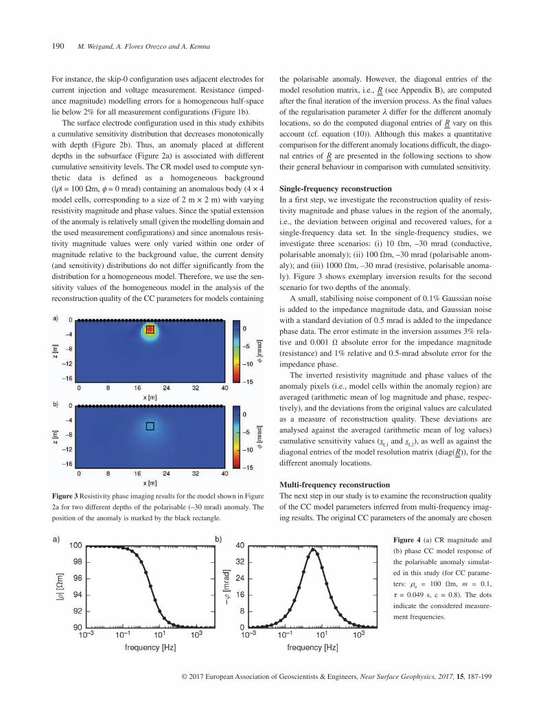
Figure 4 (a) CR magnitude and
(b) phase CC model response of
the polarisable anomaly simulat-
ed in this study (for CC parame-
ters: ρ0 = 100 Ωm, m = 0.1,
τ = 0.049 s, c = 0.8). The dots
indicate the considered measure-
ment frequencies.
Reconstruction quality of SIP parameters 191
© 2017 European Association of Geoscientists & Engineers, Near Surface Geophysics, 2017, 15, 187-199
deviation of the recovered parameters from the original CC param-eters, representing a measure of reconstruction quality:
(3)
(4)
(5)
(6)
(7)
with the subscript “orig” denoting the original CC parameters used to generate the CR response in the forward model. The
as ρ0 = 100 Ωm, m = 0.1, τ = 0.049 s , and c = 0.8, so that the peak of the phase response occurs in the center of the considered fre-quency range (at approximately 3 Hz). Based on these parameters, impedance measurements at 29 frequencies between 10-3 Hz and 104 Hz (equally spaced on a logarithmic scale) are numerically computed, as illustrated in Figure 4. The model background is set to 100 Ωm and 0 mrad for all frequencies. CR models are created for each of the 29 frequencies and used to model synthetic data-sets, which are then independently inverted. Following this, a CC model is fitted to the CR spectra extracted from the multi-frequen-cy images for each of the anomaly pixels (hereafter referred to as intrinsic spectra). Likewise, the DD is applied to the obtained intrinsic spectra. In the final step, the arithmetic mean values of the resultant spectral model parameters (log(ρ0), m, log(τ), mtot, log(τmean) are computed. Thus, for each vertical anomaly position, one set of averaged spectral model parameters is obtained.
To assess the reconstruction quality, the deviations between the recovered and original values are analysed against the sL1, sL2, and diag( ) values, averaged (arithmetic mean of log values) over the anomaly pixels. The following parameters denote the percentage
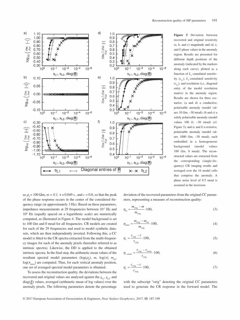
Figure 5 Deviation between
recovered and original resistivity
(a, b, and c) magnitude and (d, e,
and f) phase values in the anomaly
region. Results are presented for
different depth positions of the
anomaly (indicated by the markers
along each curve), plotted as a
function of L1 cumulated sensitiv-
ity (sL1), L2 cumulated sensitivity
(sL2), and resolution (i.e., diagonal
entry of the model resolution
matrix) in the anomaly region.
Results are shown for three sce-
narios: (a and d) a conductive,
polarisable anomaly (model val-
ues 10 Ωm, –30 mrad); (b and e) a
solely polarisable anomaly (model
values 100 Ω, –30 mrad) (cf.
Figure 3); and (c and f) a resistive,
polarisable anomaly (model val-
ues 1000 Ωm, –30 mrad), each
embedded in a homogeneous
background (model values
100 Ωm, 0 mrad). The recon-
structed values are extracted from
the corresponding (single-fre-
quency) CR imaging results and
averaged over the 16 model cells
that comprise the anomaly. A
phase noise level of 0.5 mrad is
assumed in the inversion.
M. Weigand, A. Flores Orozco and A. Kemna192
© 2017 European Association of Geoscientists & Engineers, Near Surface Geophysics, 2017, 15, 187-199
equal to the actual noise level in the phase data are assumed in the inversion, thus adequately accounting for the added noise. In subsequent inversions, the actual phase noise level is deliberately underestimated by up to one order of magnitude to investigate the effect of overfitting on the reconstruction quality.
In a final numerical simulation, we investigate the quality of reconstructed τ and τmean values for different degrees of frequen-cy dispersion (i.e., different c values) and different spectral posi-tions of the phase peak (i.e., different τ values) in the original CC model response of the anomaly.
other parameters are recovered from the CC fit and the DD of the imaging results.
A stabilising noise component of 0.1% Gaussian noise is added to the impedance magnitude data, and an impedance magnitude (resistance) error estimate comprising 3% relative error and 0.001 Ω absolute error is used in the inversions to account for numerical errors in the forward solution. Gaussian noise of different levels (0.05, 0.1, and 0.5 mrad) is added to the impedance phase datasets to investigate the effects of data noise and error estimation on the reconstruction of the CC and DD parameters. Here, at first, phase error estimates
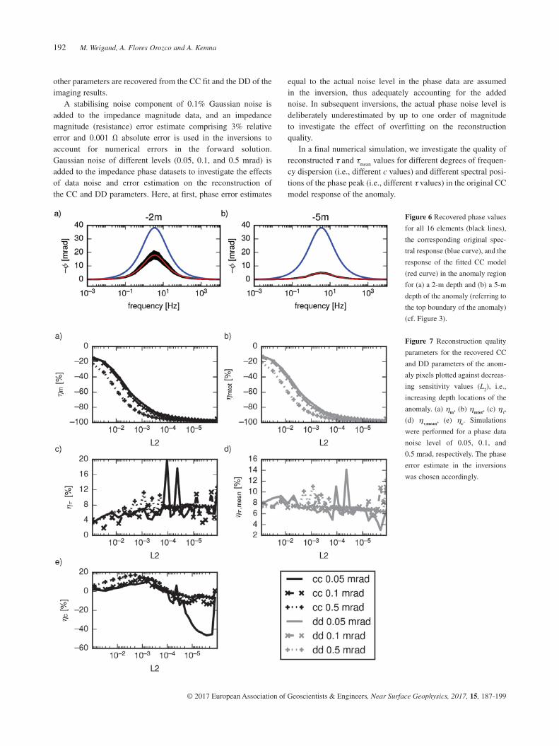
Figure 6 Recovered phase values
for all 16 elements (black lines),
the corresponding original spec-
tral response (blue curve), and the
response of the fitted CC model
(red curve) in the anomaly region
for (a) a 2-m depth and (b) a 5-m
depth of the anomaly (referring to
the top boundary of the anomaly)
(cf. Figure 3).
Figure 7 Reconstruction quality
parameters for the recovered CC
and DD parameters of the anom-
aly pixels plotted against decreas-
ing sensitivity values (L2), i.e.,
increasing depth locations of the
anomaly. (a) ηm, (b) ηmtot, (c) ητ,
(d) ητ,mean, (e) ηc. Simulations
were performed for a phase data
noise level of 0.05, 0.1, and
0.5 mrad, respectively. The phase
error estimate in the inversions
was chosen accordingly.
Reconstruction quality of SIP parameters 193
© 2017 European Association of Geoscientists & Engineers, Near Surface Geophysics, 2017, 15, 187-199
tive behaviour with respect to sensitivity (for both L1 and L2 curves) and resolution (diag( )), demonstrating that (cumulated) sensitivity is an adequate proxy to evaluate image resolution.
Multi-frequency resultsFigure 6 shows the recovered spectral phase response for the anomaly located at 2- and 5-m depths, respectively, and thus associated with different sensitivity (resolution) levels. Both reconstructed spectra exhibit an underestimation of the absolute phase values in comparison with the original values. This under-estimation is larger for the deeper anomaly position (Figure 6b) associated with lower sensitivity. An additional effect caused by the underestimated phase values is the change in the slope of the recovered phase spectrum for different depth positions, which affects the fitting of the CC exponent c (describing the degree of dispersion). This spectral distortion effect is more pronounced for the deeper anomaly position (Figure 6b), associated with regions of lower sensitivity. Intrinsic spectra recovered for the shallower anomaly position exhibit a larger spread within the anomaly (Figure 6a, black curves), indicating a stronger varia-tion of the sensitivities in the anomaly region.
Reconstruction quality of m decreases with decreasing sensi-tivity (Figure 7a), similar to the behaviour observed for the
RESULTSSingle-frequency resultsThe reconstruction quality of resistivity magnitude decreases with decreasing sensitivity for anomalies with a contrasting mag-nitude value, compared with the background magnitude (Figure 5a,c). The contrast between anomaly and background values, i.e., whether the anomaly is conductive or resistive, deter-mines the sign of the deviation, for over- or underestimated val-ues. If no contrast is present in the magnitude, reconstruction quality is independent of sensitivity (Figure 5b). The phase reconstruction curves do not show such dependence on the mag-nitude contrast (Figure 5d–f). The three cases, referring to the same value of the phase anomaly (φ = −30 mrad), reveal a mono-tonic decrease in reconstruction quality with decreasing sensitiv-ity (sL1, sL2) and resolution (diag( )) values. Reconstruction quality curves in Figure 5 also reveal a slightly different behav-iour depending on whether the anomaly is conductive or resis-tive. In particular, for the same depth position of the anomaly, a smaller deviation of the reconstructed phase values is observed in case of a conductive anomaly (Figure 5d) in comparison to a resistive anomaly (Figure 5f). This indicates an improved phase reconstruction capability in conductive regions, where current flow is focused. Furthermore, Figure 5 reveals a similar qualita-
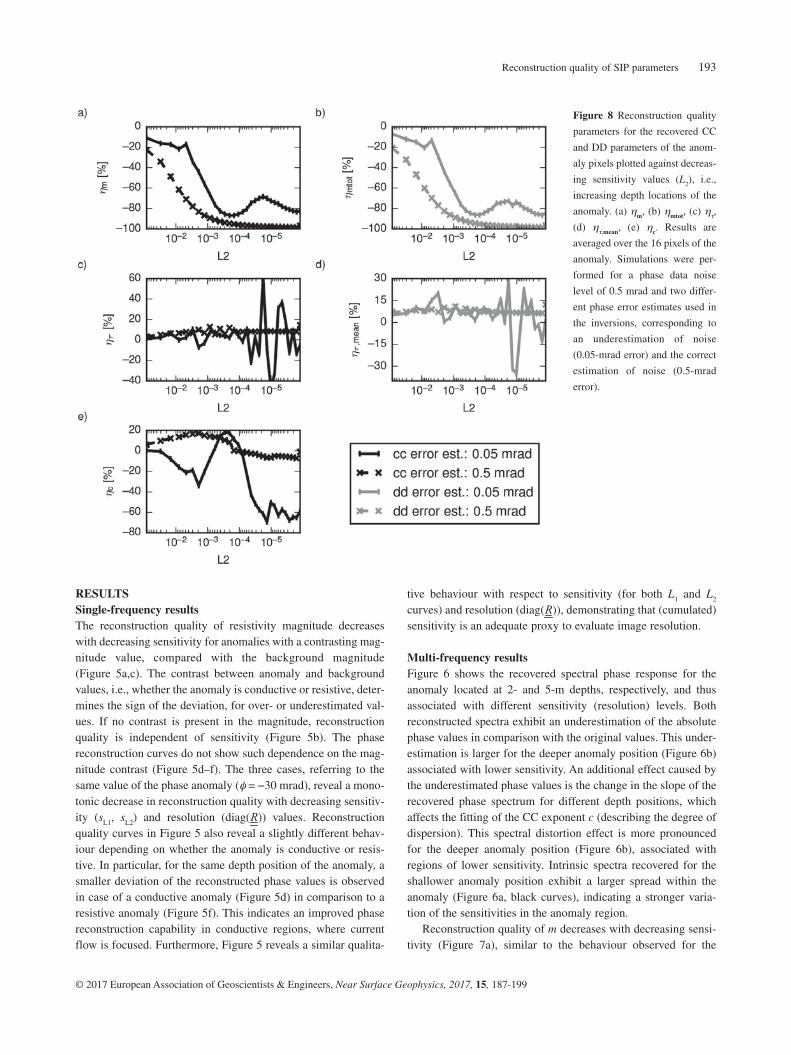
Figure 8 Reconstruction quality
parameters for the recovered CC
and DD parameters of the anom-
aly pixels plotted against decreas-
ing sensitivity values (L2), i.e.,
increasing depth locations of the
anomaly. (a) ηm, (b) ηmtot, (c) ητ,
(d) ητ,mean, (e) ηc. Results are
averaged over the 16 pixels of the
anomaly. Simulations were per-
formed for a phase data noise
level of 0.5 mrad and two differ-
ent phase error estimates used in
the inversions, corresponding to
an underestimation of noise
(0.05-mrad error) and the correct
estimation of noise (0.5-mrad
error).
M. Weigand, A. Flores Orozco and A. Kemna194
© 2017 European Association of Geoscientists & Engineers, Near Surface Geophysics, 2017, 15, 187-199
erratic behaviour for low sensitivity values below 10-4 (normal-ised L2 value), showing variations up to 20% (Figure 7c,d).
If the level of phase data noise is underestimated in the inver-sion, m and mtot reconstruction curves are shifted to smaller sensitivities, that is, for the same sensitivity (depth), the recov-ered contrast is slightly increased when noise is underestimated (on the account of overfitting the data) (Figure 8a,b). The recon-struction curves of τ and τmean become more erratic for increasing underestimation of the data noise level (Figure 8c,d), and also, c reconstruction quality decreases (Figure 8e), especially at low sensitivities. However, reconstructed relaxation time values stay within 60% of the original τ value for a ten-fold underestimation of the actual phase data noise level in the inversion.
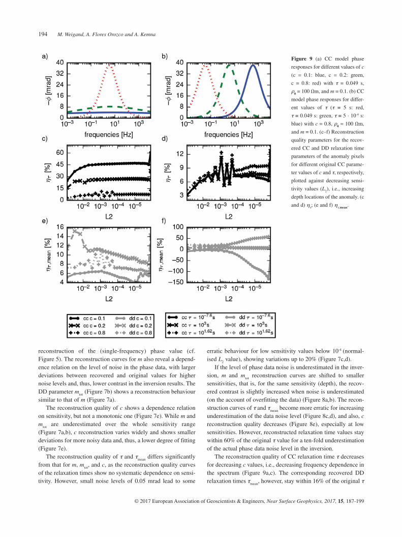
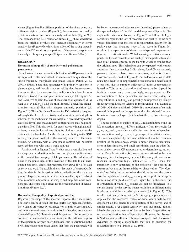
The reconstruction quality of CC relaxation time τ decreases for decreasing c values, i.e., decreasing frequency dependence in the spectrum (Figure 9a,c). The corresponding recovered DD relaxation times τmean, however, stay within 16% of the original τ
reconstruction of the (single-frequency) phase value (cf. Figure 5). The reconstruction curves for m also reveal a depend-ence relation on the level of noise in the phase data, with larger deviations between recovered and original values for higher noise levels and, thus, lower contrast in the inversion results. The DD parameter mtot (Figure 7b) shows a reconstruction behaviour similar to that of m (Figure 7a).
The reconstruction quality of c shows a dependence relation on sensitivity, but not a monotonic one (Figure 7e). While m and mtot are underestimated over the whole sensitivity range (Figure 7a,b), c reconstruction varies widely and shows smaller deviations for more noisy data and, thus, a lower degree of fitting (Figure 7e).
The reconstruction quality of τ and τmean differs significantly from that for m, mtot, and c, as the reconstruction quality curves of the relaxation times show no systematic dependence on sensi-tivity. However, small noise levels of 0.05 mrad lead to some
Figure 9 (a) CC model phase
responses for different values of c
(c = 0.1: blue, c = 0.2: green,
c = 0.8: red) with τ = 0.049 s,
ρ0 = 100 Ωm, and m = 0.1. (b) CC
model phase responses for differ-
ent values of τ (τ = 5 s: red,
τ = 0.049 s: green, τ = 5 · 10-4 s:
blue) with c = 0.8, ρ0 = 100 Ωm,
and m = 0.1. (c–f) Reconstruction
quality parameters for the recov-
ered CC and DD relaxation time
parameters of the anomaly pixels
for different original CC parame-
ter values of c and τ, respectively,
plotted against decreasing sensi-
tivity values (L2), i.e., increasing
depth locations of the anomaly. (c
and d) ητ; (e and f) ητ,mean.
Reconstruction quality of SIP parameters 195
© 2017 European Association of Geoscientists & Engineers, Near Surface Geophysics, 2017, 15, 187-199
be better reconstructed than smaller (absolute) phase values at the spectral edges of the CC model response (Figure 6). We explain the behaviour observed in Figure 7e as follows: In high-sensitivity regions, the loss of reconstruction quality for the edge values dominates over the loss of reconstruction quality for the peak values (see changing slope of the curve in Figure 5e), resulting in steeper slopes of the recovered spectral response and, thus, an overestimation of c. With decreasing sensitivity, at some point, the loss of reconstruction quality for the peak values will lead to a flattened spectral response with c values smaller than the original ones. This behaviour can be expected, with certain variations due to changing SNR values, for different anomaly parameterisations, phase error estimations, and noise levels. However, as observed in Figure 8e, an underestimation of data noise level leads to an unpredictable reconstruction behaviour of c, possibly due to stronger influence of noise components in inversion. This, in turn, has a direct influence on the slope of the intrinsic spectra and, correspondingly, on parameter c. The reconstruction of the c parameter, and to a certain extent the chargeabilities m and m
tot, can possibly be improved by using a frequency regularisation scheme in the inversion (e.g., Kemna et al. 2014; Günther and Martin 2016): If a smoothness of suitable strength is imposed on the spectrum, then its original form can be retained over a larger SNR bandwidth, i.e., down to larger depths.
The reconstruction quality of the CC relaxation time τ and the DD relaxation time τmean differ significantly from the results for ρ0, m, mtot, and c, revealing a stable, i.e., sensitivity-independent, reconstruction quality over a large range of sensitivity values. This can be explained by the direct relation of τ to the frequency position of the phase peak, which is more robust to data noise, error underestimation, and small sensitivities than the other fea-tures of the spectral CR response used to determine ρ0, m, mtot, and c. The relaxation time is (inversely) proportional to the peak frequency, i.e., the frequency at which the strongest polarisation response is observed (e.g., Pelton et al. 1978). Hence, this parameter is only dependent on the position of the peak in the spectrum, but not on the resistivity or phase values. Therefore, under/overfitting in the inversion should not impact the recon-struction quality of τ and τmean, as long as the peak in the spec-trum is not strongly distorted (cf. Figure 6). Furthermore, the interpretation of τ and τmean results will not be influenced (to a certain degree) by the varying image resolution or different noise levels, as would be the other parameters (cf. Figure 7). This result is extremely important for SIP imaging applications as it implies that the recovered relaxation time values will be less dependent on the electrode configuration of the survey and of similar quality over a large sensitivity (and thus image) region. Merely the underestimation of data noise has a larger effect on recovered relaxation times (Figure 8c,d). However, the observed 60% deviation is still relatively small compared with the overall dynamics of multiple magnitudes that can be observed for relaxation times (e.g., Pelton et al. 1978).
values (Figure 9e). For different positions of the phase peak, i.e., different original τ values (Figure 9b), the reconstruction quality of CC relaxation time does vary only within 14% (Figure 9d). The corresponding DD relaxation times τmean show deviations from the original τ values that increase enormously at lower sensitivities (Figure 9f), which is an effect of the strong depend-ence of the DD results on the position of the spectral response in the analysed frequency range (Weigand and Kemna 2016b).
DISCUSSIONReconstruction quality of resistivity and polarisation parametersTo understand the reconstruction behaviour of SIP parameters, it is important to also understand the reconstruction quality of the single-frequency magnitude and phase values. Pelton et al. (1978) already noted that parameter m is primarily sensitive to phase angle φ, and thus, it is not surprising that the reconstruc-tion curves (i.e., the reconstruction quality as a function of cumu-lated sensitivity) of m and φ are similar in shape (cf. Figures 5e and 7a,b). We explain the loss of reconstruction quality of φ (as well as of m and mtot) with the (non-linearly) decreasing signal-to-noise ratio (SNR) with deeper anomaly position (cf. Figure 2b). This effect is well known for DC resistivity imaging. Although the loss of sensitivity and resolution with depth is inherent to the method and thus inevitable, a careful design of the electrode layout and measurement configurations may help miti-gate this effect. This also holds for cross-borehole imaging appli-cations, where the loss of sensitivity/resolution is related to the distance to the boreholes. Another factor contributing to the SNR is the given phase contrast of the anomaly relative to the back-ground. An anomaly with a large phase contrast will be better resolved than one with only a weak contrast.
As observed in Figures 7 and 8, data error quantification and its adequate consideration in the inversion play a significant role in the quantitative imaging of CC parameters. The addition of noise to the phase data, or the inversion of the data to an inade-quate noise level, affects the reconstruction curve for φ (as well as for m and mtot). We explain this as the result of over/underfit-ting the data in the inversion. While underfitting the data can produce larger contrasts in the inversion results (Figure 8a,b), it also introduces artefacts in the images and amplifies noise com-ponents. This comes into effect for the reconstruction of relaxa-tion times (Figure 8c,d).
Reconstruction quality of spectral parametersRegarding the shape of the spectral response, the c reconstruc-tion curve can be divided into two parts: For high sensitivities, the c values are correctly estimated (or slightly overestimated), and below a certain sensitivity threshold value, they are underes-timated (Figure 7e). To understand this pattern, it is necessary to consider the reconstructed phase values in the different regions of the spectrum. As previously discussed, due to variations in the SNR, large (absolute) phase values that form the phase peak will
M. Weigand, A. Flores Orozco and A. Kemna196
© 2017 European Association of Geoscientists & Engineers, Near Surface Geophysics, 2017, 15, 187-199
with respect to different noise levels in the data; however, it is important that the considered frequency range is wide enough to capture the spectral behaviour. Hence, we also conclude that the quality of the reconstruction will benefit from the acquisi-tion of broadband CR measurements, preferably with dense spectral sampling.
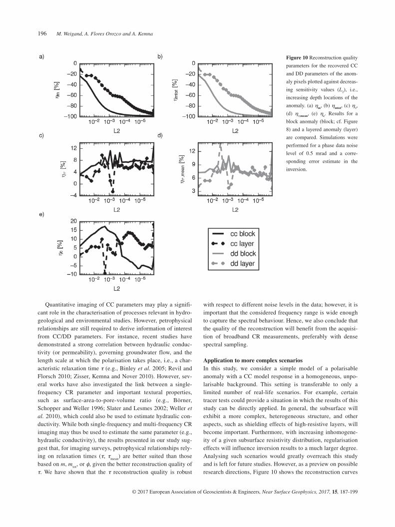
Application to more complex scenariosIn this study, we consider a simple model of a polarisable anomaly with a CC model response in a homogeneous, unpo-larisable background. This setting is transferable to only a limited number of real-life scenarios. For example, certain tracer tests could provide a situation in which the results of this study can be directly applied. In general, the subsurface will exhibit a more complex, heterogeneous structure, and other aspects, such as shielding effects of high-resistive layers, will become important. Furthermore, with increasing inhomogene-ity of a given subsurface resistivity distribution, regularisation effects will influence inversion results to a much larger degree. Analysing such scenarios would greatly overreach this study and is left for future studies. However, as a preview on possible research directions, Figure 10 shows the reconstruction curves
Quantitative imaging of CC parameters may play a signifi-cant role in the characterisation of processes relevant in hydro-geological and environmental studies. However, petrophysical relationships are still required to derive information of interest from CC/DD parameters. For instance, recent studies have demonstrated a strong correlation between hydraulic conduc-tivity (or permeability), governing groundwater flow, and the length scale at which the polarisation takes place, i.e., a char-acteristic relaxation time τ (e.g., Binley et al. 2005; Revil and Florsch 2010; Zisser, Kemna and Nover 2010). However, sev-eral works have also investigated the link between a single-frequency CR parameter and important textural properties, such as surface-area-to-pore-volume ratio (e.g., Börner, Schopper and Weller 1996; Slater and Lesmes 2002; Weller et al. 2010), which could also be used to estimate hydraulic con-ductivity. While both single-frequency and multi-frequency CR imaging may thus be used to estimate the same parameter (e.g., hydraulic conductivity), the results presented in our study sug-gest that, for imaging surveys, petrophysical relationships rely-ing on relaxation times (τ, τmean) are better suited than those based on m, mtot, or φ, given the better reconstruction quality of τ. We have shown that the τ reconstruction quality is robust
Figure 10 Reconstruction quality
parameters for the recovered CC
and DD parameters of the anom-
aly pixels plotted against decreas-
ing sensitivity values (L2), i.e.,
increasing depth locations of the
anomaly. (a) ηm, (b) ηmtot, (c) ητ,
(d) ητ,mean, (e) ηc. Results for a
block anomaly (block; cf. Figure
8) and a layered anomaly (layer)
are compared. Simulations were
performed for a phase data noise
level of 0.5 mrad and a corre-
sponding error estimate in the
inversion.
Reconstruction quality of SIP parameters 197
© 2017 European Association of Geoscientists & Engineers, Near Surface Geophysics, 2017, 15, 187-199
relationships, is also possible in a multi-frequency CR imaging framework. The recovery of chargeabilities m or mtot, as well as the CC exponent c, on the other hand, is highly affected by the imaging characteristics (sensitivity, resolution), which must be carefully taken into account if a quantitative interpretation is intended. Given the strong correlation between CC model parameters (and corresponding DD parameters) and various petrophysical properties of relevance in hydrogeological and environmental applications, as demonstrated by a large number of studies over the last years, our findings are of outermost importance for the successful quantitative application of multi-frequency CR imaging for improved subsurface characterisation.
ACKNOWLEDGEMENTSParts of this work were conducted in the framework of the SFB TR32 “Patterns in soil-vegetation-atmosphere systems: monitor-ing, modeling and data assimilation” funded by the Deutsche Forschungsgemeinschaft (DFG). The authors would like to thank the two anonymous referees for their very constructive reviews.
REFERENCESAbdel Aal G.Z., Atekwana E.A., Slater L.D. and Atekwana E.A. 2004.
Effects of microbial processes on electrolytic and interfacial electrical properties of unconsolidated sediments. Geophysical Research Letters 31(12).
Alumbaugh D.L. and Newman G.A. 2000. Image appraisal for 2-D and 3-D electromagnetic inversion. Geophysics 65(5), 1455–1467.
Atekwana E.A. and Slater L.D. 2009. Biogeophysics: a new frontier in earth science research. Reviews of Geophysics 47(4).
Binley A. and Kemna A. 2005. DC resistivity and induced polarization methods. In: Hydrogeophysics (eds Y. Rubin and S. Hubbard), pp. 129–156. Netherlands: Springer.
Binley A., Slater L.D., Fukes M. and Cassiani G. 2005. Relationship between spectral induced polarization and hydraulic properties of saturated and unsaturated sandstone. Water Resources Research 41(12), 1–13.
Börner F.D., Schopper J.R. and Weller A. 1996. Evaluation of transport and storage properties in the soil and groundwater zone from induced polarization measurements. Geophysical Prospecting 44(4), 583–601.
Cole K.S. and Cole R.H. 1941. Dispersion and absorption in dielectrics I. Alternating current characteristics. Journal of Chemical Physics 9(4), 341–351.
Davis C.A., Atekwana E., Atekwana E., Slater L.D., Rossbach S. and Mormile M.R. 2006. Microbial growth and biofilm formation in geo-logic media is detected with complex conductivity measurements. Geophysical Research Letters 33(18).
Day-Lewis F.D., Singha K. and Binley A.M. 2005. Applying petrophysi-cal models to radar travel time and electrical resistivity tomograms: resolution-dependent limitations. Journal of Geophysical Research 110(B8).
Flores Orozco A., Williams K.H., Long P.E., Hubbard S.S. and Kemna A. 2011. Using complex resistivity imaging to infer biogeochemical processes associated with bioremediation of an uranium-contaminated aquifer. Journal of Geophysical Research 116(G3).
Flores Orozco A., Kemna A., Oberdörster C., Zschornack L., Leven C., Dietrich P. et al. 2012a. Delineation of subsurface hydrocarbon contamination at a former hydrogenation plant using spectral induced polarization imaging. Journal of Contaminant Hydrology 136, 131–144.
of CC and DD parameters for a setting similar to the one pre-sented in Figure 7. Data noise with a standard deviation of 0.5 mrad is added to the data, and the corresponding error esti-mates are used in the inversion. Intrinsic spectra are extracted from 2 m × 2 m areas successively moved to deeper locations, as is done in the previous simulations. However, instead of considering a local anomalous block, the whole depth layer is parameterised with a given CC model response. Thus, a simple layered structure is simulated, as for example found when sedimentary layers are investigated. Intrinsic spectra are only extracted from the center of the modelling grid to exclude boundary effects of the regularisation. The reconstruction of m and mtot is greatly improved over the non-layered case (Figure 10a,b), while relaxation times do not show large varia-tions (below 10%) from each other (Figure 10c,d). Merely c reconstruction shows differences in its reconstruction behav-iour (Figure 10e), whose origin is not yet clear and must be addressed in future work.
We believe that our results on the reconstruction quality of CC and DD parameters as a function of sensitivity are still applicable to more heterogeneous situations, at least if the given spectral signatures are close to the CC type. Hence, considering our results, we can also suggest that sensitivity values can be used to assess the reliability of the reconstructed parameters in single- and multi-frequency CR imaging. Our results also show that (cumulated) sensitivity can be a sufficient parameter to address reconstruction quality, compared with other computationally more expensive approaches based on a resolution matrix.
CONCLUSIONSWe investigated the reconstruction quality of CC model and DD parameters based on multi-frequency CR imaging by means of numerical simulations. Our results show that the reconstruction quality of CC parameters m and c, as well as of DD parameter m
tot, vary strongly across the imaging plane, with reconstructed values deviating considerably from the original values for lower sensitivities. The reconstruction quality of m and mtot decreases monotonically with decreasing sensitivity, while c shows incon-clusive behaviour that cannot be explained yet for all scenarios. The same dependence in the reconstruction quality curves is observed for the diagonal entries of the model resolution matrix. Therefore, based on our results, cumulated sensitivity (regardless of whether its L1 or its L2 measure is used) appears to be an adequate, computationally inexpensive proxy for image resolu-tion. Opposite to this, the reconstruction quality of CC relaxation time τ and DD relaxation time τmean is only weakly dependent on sensitivity, resulting in fair quantitative reconstructions even in regions with relatively low sensitivity (deviation less than 20% from the original value down to normalised L2 cumulated sensi-tivity values of 10-4).
Our results suggest that a quantitative interpretation of relaxa-tion time parameters (either from CC model fit or DD), and any parameters derived from them using established petrophysical

M. Weigand, A. Flores Orozco and A. Kemna198
© 2017 European Association of Geoscientists & Engineers, Near Surface Geophysics, 2017, 15, 187-199
Revil A. and Florsch N. 2010. Determination of permeability from spectral induced polarization in granular media. Geophysical Journal International 181(3), 1480–1498.
Slater L. 2007. Near surface electrical characterization of hydraulic conductivity: from petrophysical properties to aquifer geometries—a review. Surveys in Geophysics 28(2-3), 169–197.
Slater L. and Lesmes D.P. 2002. Electrical-hydraulic relationships observed for unconsolidated sediments. Water Resources Research 38(10), 31-1 – 31-13.
Slater L. and Binley A. 2006. Synthetic and field-based electrical imag-ing of a zerovalent iron barrier: implications for monitoring long-term barrier performance. Geophysics 71(5), B129–B137.
Vanhala H. 1997. Mapping oil-contaminated sand and till with the spectral induced polarization (SIP) method. Geophysical Prospecting 45(2), 303–326.
Weigand M. and Kemna A. 2016a. Multi-frequency electrical imped-ance tomography as a non-invasive tool to characterize and monitor crop root systems. Biogeosciences Discussions 2016, 1–31. http://www.biogeosciences-discuss.net/bg-2016-154/.
Weigand M. and Kemna A. 2016b. Debye decomposition of time-lapse spectral induced polarisation data. Computers and Geosciences 86, 34–45.
Weigand M. and Kemna A. 2016c. Relationship between Cole–Cole model parameters and spectral decomposition parameters derived from SIP data. Geophysical Journal International 205, 1414– 1419.
Weller A., Slater L., Nordsiek S. and Ntarlagiannis D. 2010. On the estimation of specific surface per unit pore volume from induced polarization: a robust empirical relation fits multiple data sets. Geophysics 75(4), WA105–WA112.
Williams K.H., Kemna A., Wilkins M.J., Druhan J., Arntzen E., N’Guessan A.L. et al. 2009. Geophysical monitoring of coupled microbial and geochemical processes during stimulated subsurface bioremediation. Environmental Science & Technology 43(17), 6717–6723.
Zanetti C., Weller A., Vennetier M. and Mériaux P. 2011. Detection of buried tree root samples by using geoelectrical measurements: a laboratory experiment. Plant and Soil 339(1-2), 273–283.
Zisser N., Kemna A. and Nover G. 2010. Relationship between low-frequency electrical properties and hydraulic permeability of low-
permeability sandstones. Geophysics 75(3), E131–E141.
APPENDIXA. Complex resistivity inversionCR images are computed using the inversion code of Kemna (2000). The code computes the distribution of CR ρ (expressed in magnitude (|ρ|) and phase (φ)), in a 2D (x, z) image plane from a given dataset of complex transfer impedances Z
i (expressed in
magnitude (|Zi|) and phase (φ
i)) under the constraint of maximum
smoothness. The algorithm iteratively minimises a cost function Ψ(m), which is composed of the measures of data misfit and model roughness, with both terms being balanced by a (real-valued) regularisation parameter λ:
(8)
where d is the data vector (log impedance data), m is the model parameter vector (log complex resistivities of parameter cells (lumped elements of underlying finite-element mesh)), f(m)is the operator of the forward model, is a data weighting matrix,
Flores Orozco A., Kemna A. and Zimmermann E. 2012b. Data error quantification in spectral induced polarization imaging. Geophysics 77(3), E227–E237.
Flores Orozco A., Williams K.H. and Kemna A. 2013. Time-lapse spec-tral induced polarization imaging of stimulated uranium bioremedia-tion. Near Surface Geophysics 11(5), 531–544.
Flores Orozco A., Velimirovic M., Tosco T., Kemna A., Sapion H., Klaas N. et al. 2015. Monitoring the injection of microscale zerova-lent iron particles for groundwater remediation by means of complex electrical conductivity imaging. Environmental Science & Technology 49(9), 5593–5600.
Florsch N., Revil A. and Camerlynck C. 2014. Inversion of generalized relaxation time distributions with optimized damping parameter. Journal of Applied Geophysics 109, 119–132.
Friedel S. 2003. Resolution, stability and efficiency of resistivity tomography estimated from a generalized inverse approach. Geophysical Journal International 153(2), 305–316.
Günther T. and Martin T. 2016. Spectral two-dimensional inversion of frequency-domain induced polarization data from a mining slag heap. Journal of Applied Geophysics 135, 436-448.
Hördt A., Blaschek R., Kemna A. and Zisser N. 2007. Hydraulic con-ductivity estimation from induced polarisation data at the field scale—the Krauthausen case history. Journal of Applied Geophysics 62(1), 33–46.
Kemna A. 2000. Tomographic inversion of complex resistivity—theory and application. PhD thesis, Ruhr-Universität Bochum, Germany.
Kemna A., Vanderborght J., Kulessa B., and Vereecken H. 2002. Imaging and characterisation of subsurface solute transport using electrical resistivity tomography (ERT) and equivalent transport models, Journal of Hydrology 267, 125–146.
Kemna A., Binley A. and Slater L. 2004. Crosshole IP imaging for engi-neering and environmental applications. Geophysics 69(1), 97–107.
Kemna A., Binley A., Cassiani G., Niederleithinger E., Revil A., Slater L. et al. 2012. An overview of the spectral induced polarization method for near-surface applications. Near Surface Geophysics 10(6), 453–468.
Kemna A., Huisman J.A., Zimmermann E., Martin R., Zhao Y., Treichel A. et al. 2014. Broadband electrical impedance tomography for subsurface characterization using improved corrections of elec-tromagnetic coupling and spectral regularization. In: Tomography of the Earth’s Crust: From Geophysical Sounding to Real-Time Monitoring, pp. 1–20. Springer.
Lesmes D.P. and Morgan F.D. 2001. Dielectric spectroscopy of sedi-mentary rocks. Journal of Geophysical Research 106(B7), 13329–13346.
Luo Y. and Zhang G. 1998. Theory and Application of Spectral Induced Polarization. Tulsa: Society of Exploration Geophysicists.
Mwakanyamale K., Slater L., Binley A. and Ntarlagiannis D. 2012. Lithologic imaging using complex conductivity: lessons learned from the Hanford 300 Area. Geophysics 77(6), E397–E409.
Nguyen F., Kemna A., Antonsson A., Engesgaard P., Kuras O., Ogilvy R. et al. 2009. Characterization of seawater intrusion using 2D elec-trical imaging. Near Surface Geophysics 7(5-6), 377– 390.
Nordsiek S. and Weller A. 2008. A new approach to fitting induced-polarization spectra. Geophysics 73(6), F235–F245.
Ntarlagiannis D., Williams K.H., Slater L. and Hubbard S. 2005. Low-frequency electrical response to microbial induced sulfide precipita-tion. Journal of Geophysical Research 110(G02009).
Oldenburg D.W. and Li Y. 1999. Estimating depth of investigation in DC resistivity and IP surveys. Geophysics 64(2), 403–416.
Pelton W.H., Ward S.H., Hallof P.G., Sill W.R. and Nelson P.H. 1978. Mineral discrimination and removal of inductive coupling with mul-tifrequency IP. Geophysics 43(3), 588–609.
Reconstruction quality of SIP parameters 199
© 2017 European Association of Geoscientists & Engineers, Near Surface Geophysics, 2017, 15, 187-199
matrix, (e.g., Alumbaugh and Newman 2000), which, for the complex case, is given by
(10)
where is the complex Jacobian matrix (for its com- putation, see Kemna (2000)). The model resolution matrix is usually evaluated at the end of the iterative inversion process. Due to its lower computational cost compared with , the cumu-lative (and error-weighted) sensitivity, sL2, has been alternatively used (e.g., Kemna et al. 2002; Nguyen et al. 2009). Using the L2-norm, its components are given by Kemna (2000) as
(11)
where aik is the i,kth element of the Jacobian matrix , i.e., the sensitivity of the ith datum with respect to the kth parameter cell. Note that also for the complex case, sL2 is a real-valued vector. The cumulated sensitivity is a measure of how much an entire dataset changes due to a changing model cell. Given the corre-spondence between cumulated sensitivity and the diagonal of the model resolution matrix, the cumulated sensitivity can be used as a proxy for model resolution. We emphasise here that a large cumulated sensitivity does not necessarily imply a good resolu-tion; however, good resolution cannot be expected for model cells exhibiting small cumulative sensitivities (Kemna 2000).
In addition to the L2-normed cumulated sensitivity, in our study, we also compute the L1-normed cumulated sensitivity based on the sum of the absolute values of the sensitivities (weighted by the absolute error of the corresponding measurement):
(12)
and is a (real-valued) matrix evaluating the first-order rough-ness of m. Under the assumption that the data errors are uncor-related and normally distributed, is a diagonal matrix given by
(9)
where i is the complex error estimate (standard deviation) of the
ith datum, i.e., (with j denoting the imaginary unit). At each iteration step of the inversion, a univariate search is performed to find the maximum value of the regularisation parameter λ that locally minimises the data misfit.
In CR inversion, the data misfit is typically dominated by the real component of the complex data (that is log impedance mag-nitude). To properly take into account the misfit in the phase (imaginary component of the data), subsequent to the complex inversion, additional inversion iterations are run only for the phase (i.e., as a real-valued inverse problem with the impedance phase values as data and the CR phase values as parameters). Here, the resistivity magnitude image from the complex inver-sion is kept unchanged, and the same smoothness-constrained inversion procedure is used. For more details on the implementa-tion of the inversion, we refer to Kemna (2000).
B. Image appraisalElectrical resistivity images exhibit a variable spatial resolution (e.g., Oldenburg and Li 1999; Friedel 2003; Binley and Kemna 2005). A common approach for the quantification of this variable resolution uses the diagonal entries of the model resolution


![[MS-SIP]: Session Initiation Protocol ExtensionsMS-SIP]-160714.pdf · [MS-SIP]: Session Initiation Protocol Extensions ... sip. . . .](https://img.pdfslide.us/doc/110x75/5f144311cb0953247f1ddd57/ms-sip-session-initiation-protocol-extensions-ms-sip-160714pdf-ms-sip.jpg)


![[MS-SIP]: Session Initiation Protocol ExtensionsMS-SIP].pdfSession Initiation Protocol Extensions SIP. . SIP message.](https://img.pdfslide.us/doc/110x75/5e7f8669844925290d6f8357/ms-sip-session-initiation-protocol-extensions-ms-sippdf-session-initiation.jpg)