Reconstruction from Projections

1

Based on

SPECT reconstruction

Martin Šámal

Charles University Prague, Czech Republic

[email protected]

Reconstruction from Projections

M.C. Villa UriolComputational Imaging Lab

email: [email protected]: http://www.cilab.upf.edu

Tomography is performed in 2 steps:

1st step = data acquisition (record of projections)

The result is a set of angular projections.

The set of projections of a single slice is called sinogram.

2nd step = image recontruction from projections

There are 2 groups of reconstruction methods:

analytic (e.g. FBP = filtered back projection) and

iterative (e.g. ART = algebraic reconstruction

techniques).

www.Vidyarthiplus.com


2

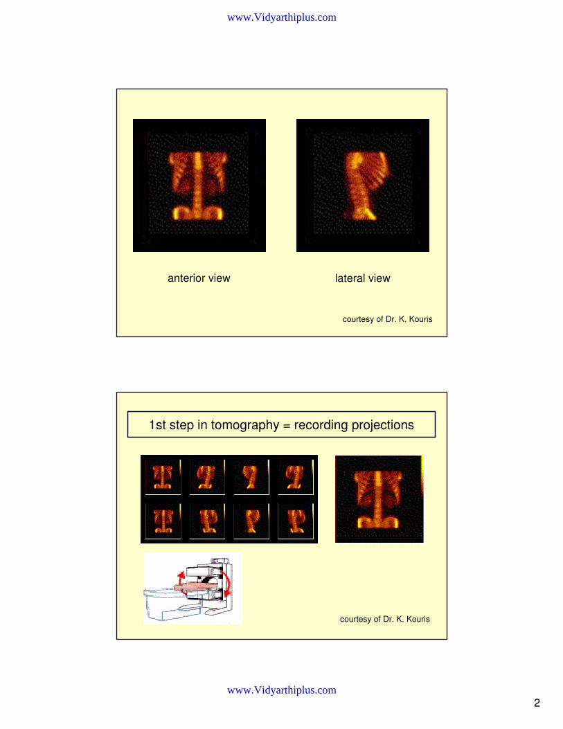
anterior view lateral view

courtesy of Dr. K. Kouris

1st step in tomography = recording projections




3

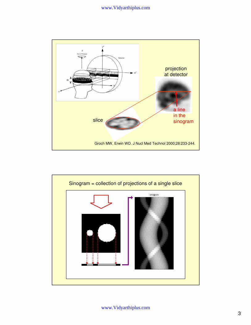
Groch MW, Erwin WD. J Nucl Med Technol 2000;28:233-244.

slice

projectionat detector

a line in the sinogram

Sinogram = collection of projections of a single slice



4

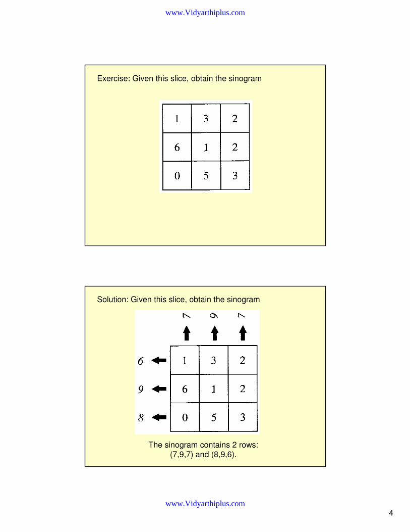
Exercise: Given this slice, obtain the sinogram

Solution: Given this slice, obtain the sinogram

The sinogram contains 2 rows:(7,9,7) and (8,9,6).



5

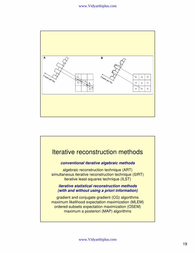
2nd step in tomography = reconstruction from projections

Analytic reconstruction methods (e.g. the filtered back-projection algorithm) are efficient (fast) and elegant, but they are unable to handle complicated factors such as scatter. Filtered back projection has been used for reconstructions in x-ray CT and for most SPECT and PET reconstructions until recently.

Iterative reconstruction algorithms, on the other hand, are more versatile but less efficient. Efficient (that is - fast) iterative algorithms are currently under development. With rapid increases being made in computer speed and memory, iterative reconstruction algorithms will be used in more and more applications of SPECT and PET and will enable more quantitative reconstructions.

Analytic reconstruction methods(projection - backprojection algorithms)

filtered back-projection

back-projection filtering

Radon J.

On the determination of functions from their integrals along certain manifolds [in German].

Math Phys Klass 1917;69:262-277.



6

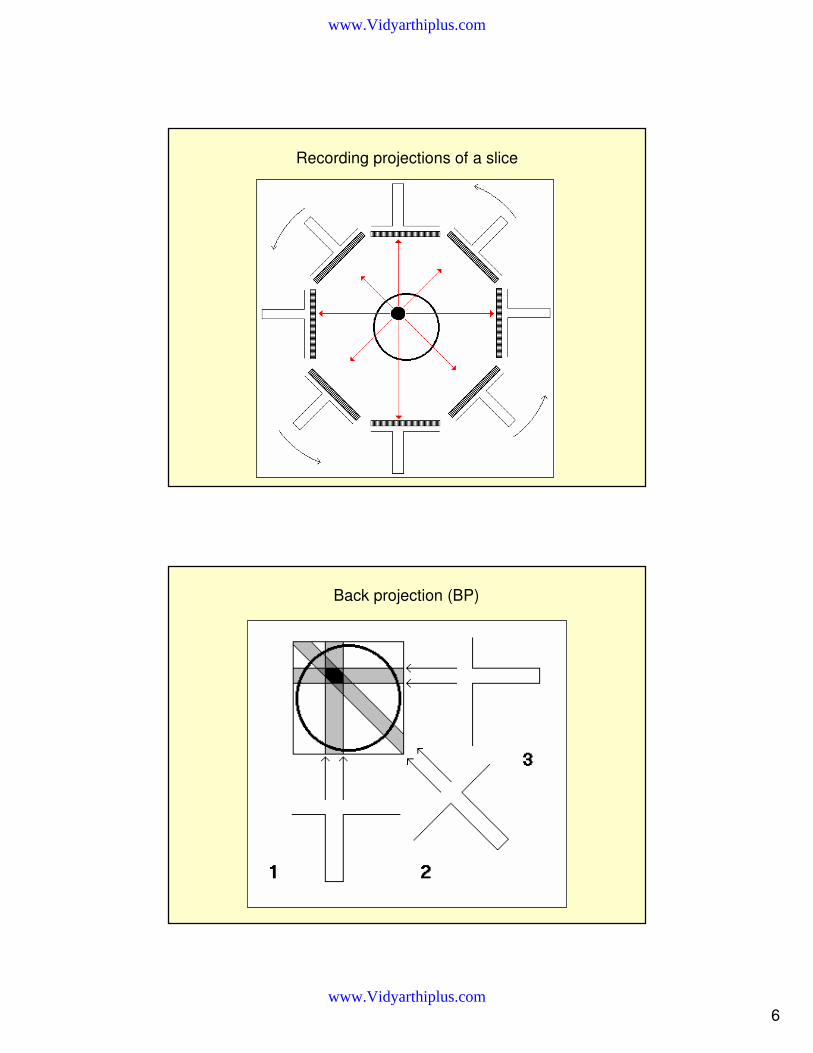
Recording projections of a slice

Back projection (BP)



7

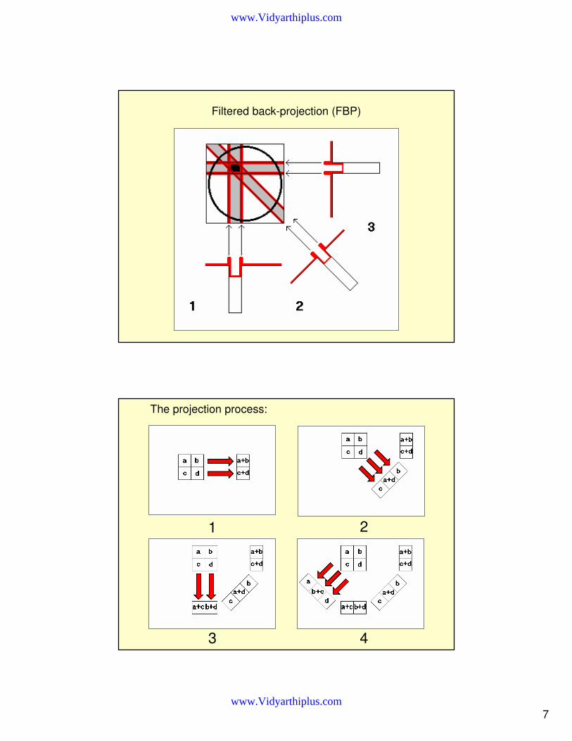
Filtered back-projection (FBP)

1 2

3 4

The projection process:



8

Reconstruction problem

1 2

3 4

The backprojection algorithm



9

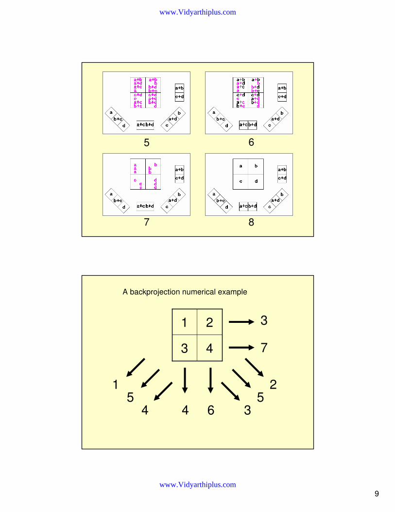
5 6

7 8

43

21 3

7

4 6

25

3

15

4

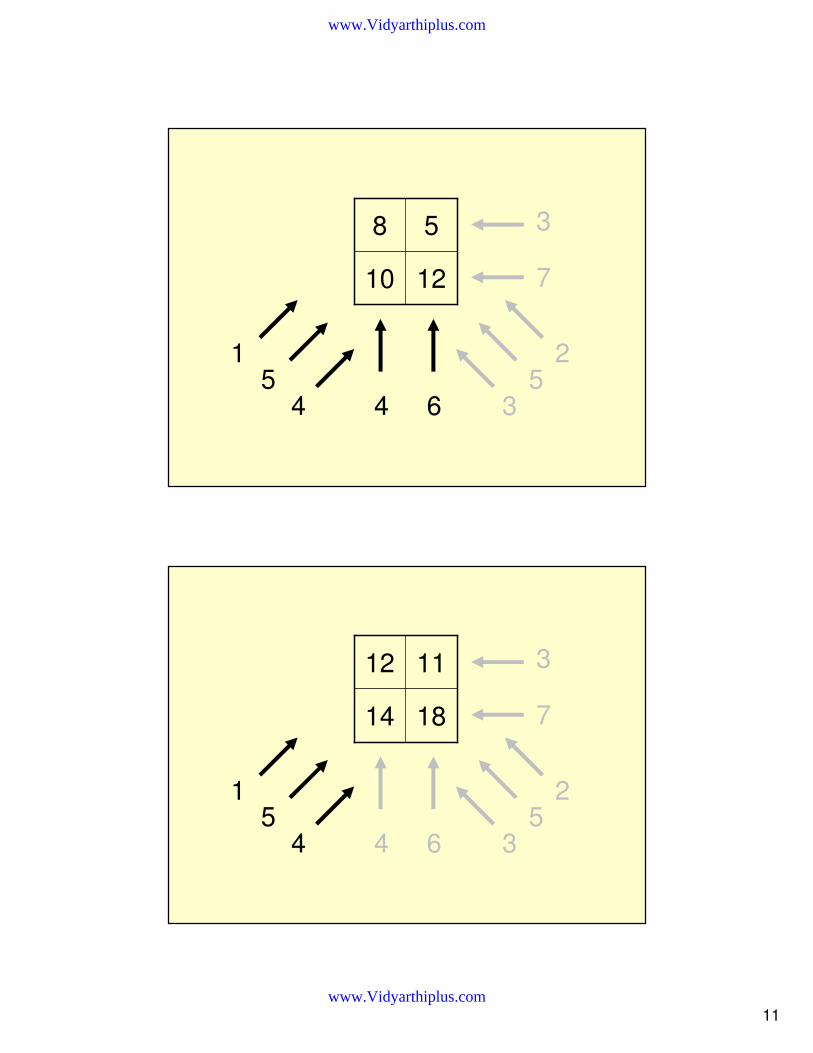
A backprojection numerical example



10

00

00 3

7

4 6

25

3

15

4

77

33 3

7

4 6

25

3

15

4



11

1210

58 3

7

4 6

25

3

15

4

1814

1112 3

7

4 6

25

3

15

4



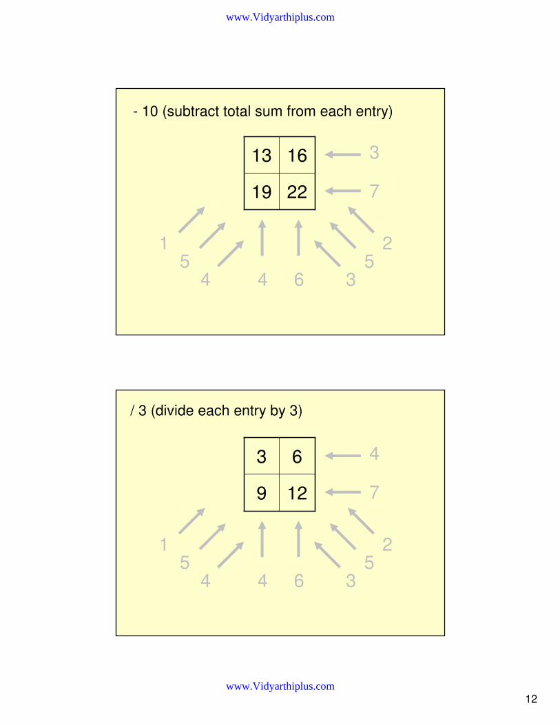
12

2219

1613 3

7

4 6

25

3

15

4

- 10 (subtract total sum from each entry)

129

63 4

7

4 6

25

3

15

4

/ 3 (divide each entry by 3)



13

43

21 4

7

4 6

25

3

15

4



14

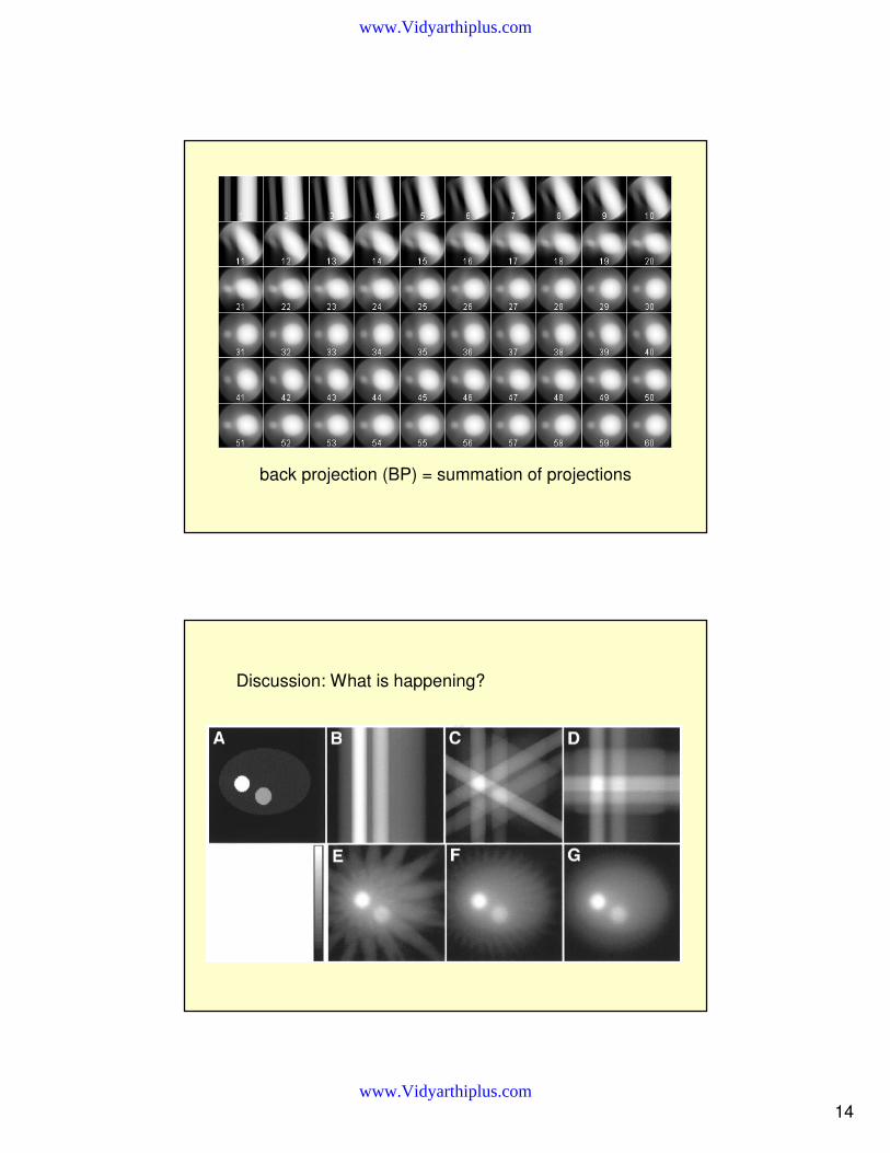
back projection (BP) = summation of projections

Discussion: What is happening?



15

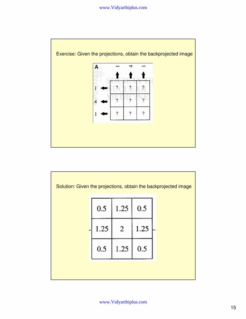
Exercise: Given the projections, obtain the backprojected image

Solution: Given the projections, obtain the backprojected image



16

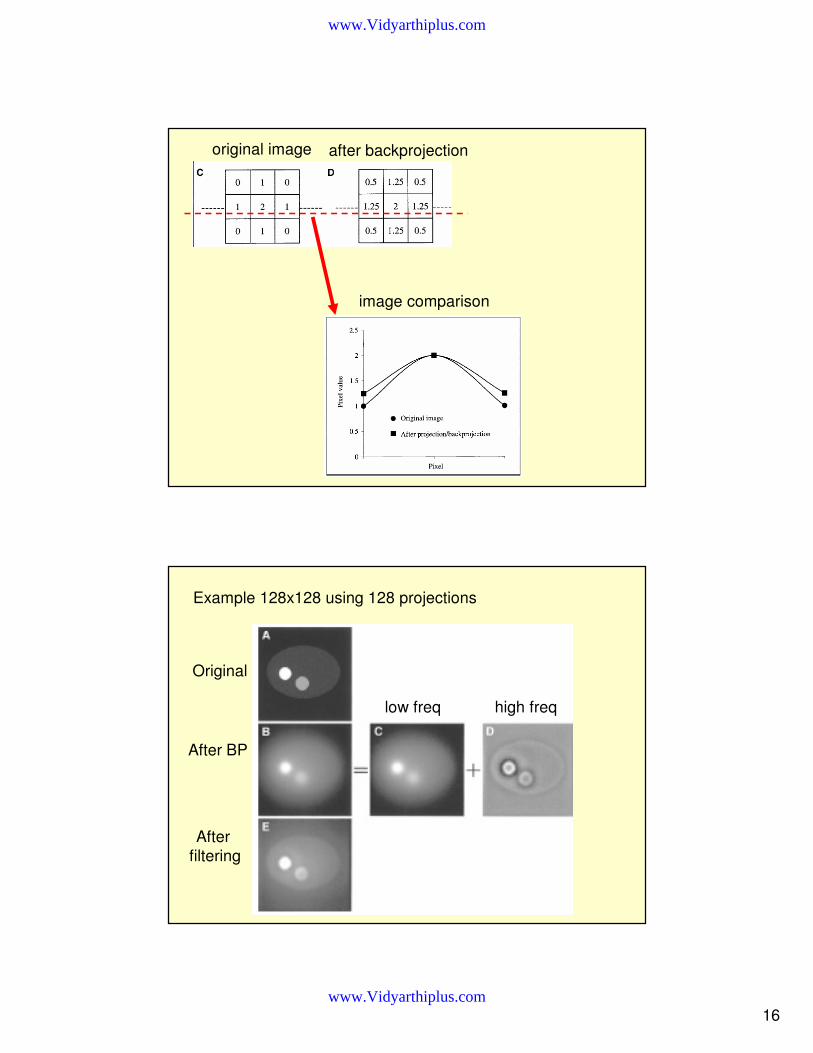
original image after backprojection

image comparison

Example 128x128 using 128 projections

Original

After BP

After filtering

low freq high freq



17

filtered back projection (FBP)

back projection filtered back projection

Sequence of summing original and filtered projections



18

y

z

x

x-position

Count rate

z

y

Reconstruction of a slice from projectionsexample = myocardial perfusion, left ventricle, long axis


Reconstruction of a slice from projectionsexample = myocardial perfusion, left ventricle, long axis




19

Iterative reconstruction methods

conventional iterative algebraic methods

algebraic reconstruction technique (ART) simultaneous iterative reconstruction technique (SIRT)

iterative least-squares technique (ILST)

iterative statistical reconstruction methods (with and without using a priori information)

gradient and conjugate gradient (CG) algorithms maximum likelihood expectation maximization (MLEM)

ordered-subsets expectation maximization (OSEM) maximum a posteriori (MAP) algorithms



20

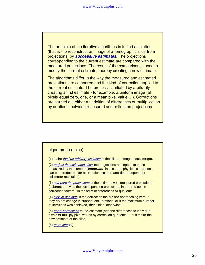
The principle of the iterative algorithms is to find a solution (that is - to reconstruct an image of a tomographic slice from projections) by successive estimates. The projections corresponding to the current estimate are compared with the measured projections. The result of the comparison is used to modify the current estimate, thereby creating a new estimate.

The algorithms differ in the way the measured and estimated projections are compared and the kind of correction applied to the current estimate. The process is initiated by arbitrarily creating a first estimate - for example, a uniform image (all pixels equal zero, one, or a mean pixel value,…). Corrections are carried out either as addition of differences or multiplication by quotients between measured and estimated projections.

algorithm (a recipe)

(1) make the first arbitrary estimate of the slice (homogeneous image),

(2) project the estimated slice into projections analogous to those measured by the camera (important: in this step, physical corrections can be introduced - for attenuation, scatter, and depth-dependent collimator resolution),

(3) compare the projections of the estimate with measured projections (subtract or divide the corresponding projections in order to obtain correction factors - in the form of differences or quotients),

(4) stop or continue: if the correction factors are approaching zero, if they do not change in subsequent iterations, or if the maximum number of iterations was achieved, then finish; otherwise

(5) apply corrections to the estimate (add the differences to individual pixels or multiply pixel values by correction quotients) - thus make the new estimate of the slice,

(6) go to step (2).



21

measured projections

first estimate

and its projections

correction factors (differences between projections)

first iteration

(additive corrections)

second iteration

(additive corrections)

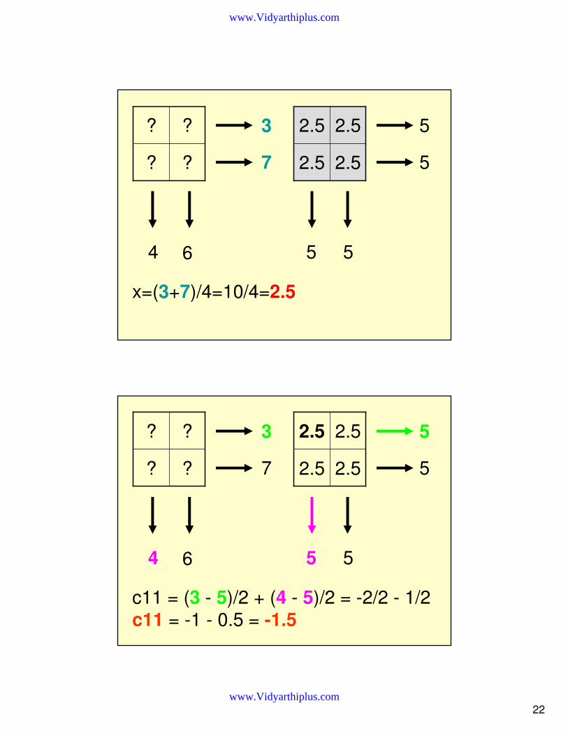
x=(a+b+c+d)/4

An ART first algorithm

43

21 3

7

4 6

Original data

Example: Use the proposed ART algorithm



22

??

?? 3

7

4 6

2.52.5

2.52.5 5

5

5 5

x=(3+7)/4=10/4=2.5

??

?? 3

7

4 6

2.52.5

2.52.5 5

5

5 5

c11 = (3 - 5)/2 + (4 - 5)/2 = -2/2 - 1/2 c11 = -1 - 0.5 = -1.5



23

??

?? 3

7

4 6

2.52.5

2.51 5

5

5 5

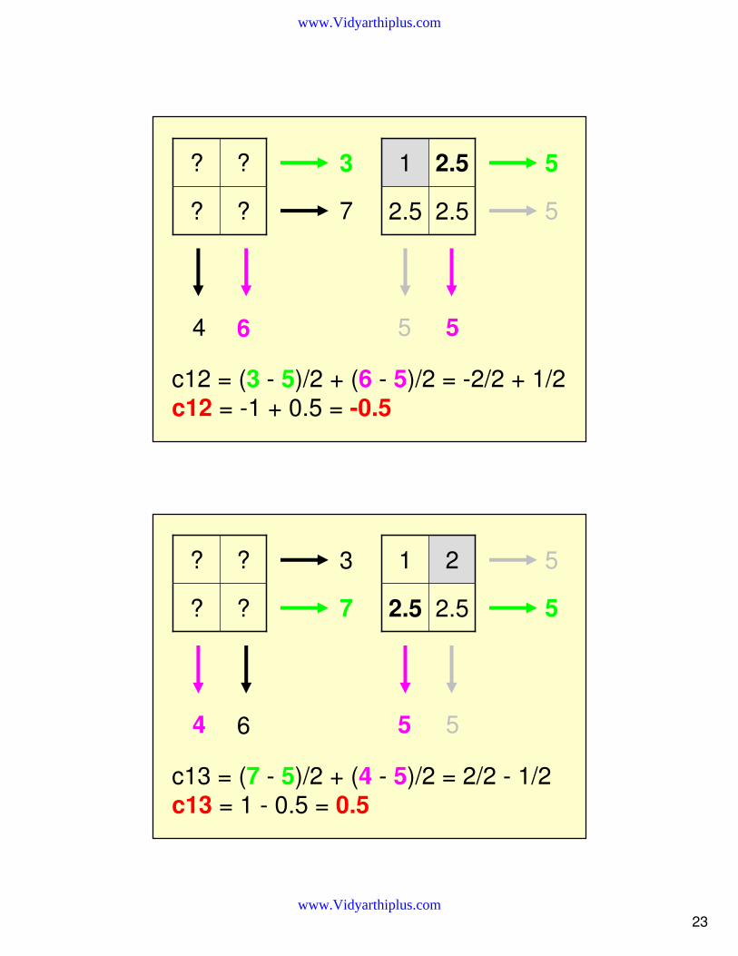
c12 = (3 - 5)/2 + (6 - 5)/2 = -2/2 + 1/2 c12 = -1 + 0.5 = -0.5

??

?? 3

7

4 6

2.52.5

21 5

5

5 5

c13 = (7 - 5)/2 + (4 - 5)/2 = 2/2 - 1/2 c13 = 1 - 0.5 = 0.5



24

??

?? 3

7

4 6

2.53

21 5

5

5 5

c14 = (7 - 5)/2 + (6 - 5)/2 = 2/2 + 1/2 c14 = 1 + 0.5 = 1.5

43

21 3

7

4 6

43

21 5

5

5 5

Original data Reconstructed data



25

measured projections

first estimate

and its projections

correction factors (quotients between projections)

first iteration

(multiplicat. corrections)

second iteration (multiplicat. corrections)

x=(a+b+c+d)/4

c11=(p01/p11)

*(p03/p13)

c12=(p01/p11)

*(p04/p14)

c13=(p02/p12)

*(p03/p13)

c14=(p02/p12)

*(p04/p14)

c11=(p01/p11)

*(p03/p13)

c12=(p01/p11)

*(p04/p14)

c13=(p02/p12)

*(p03/p13)

c14=(p02/p12)

*(p04/p14)

c11=(p01/p11)

*(p03/p13)

c12=(p01/p11)

*(p04/p14)

c13=(p02/p12)

*(p03/p13)

c14=(p02/p12)

*(p04/p14)

A multiplicative approach (MART)

43

21 3

7

4 6

Original data

Exercise: Apply MART algorithm



26

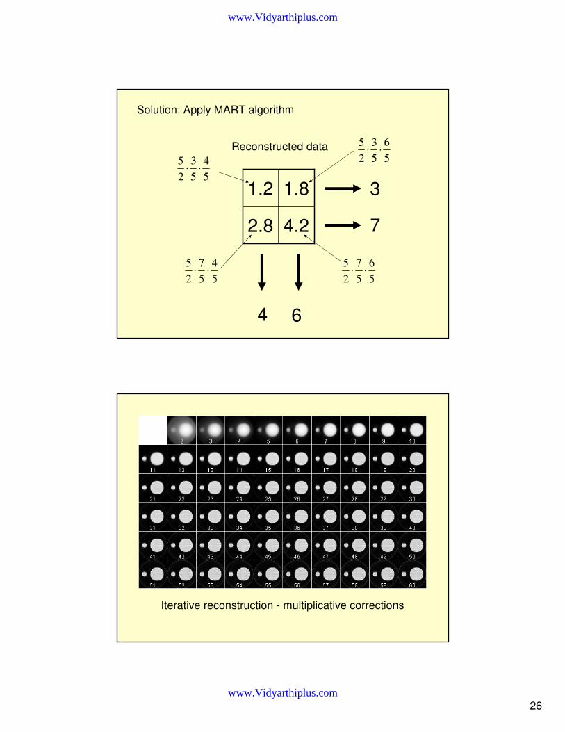
Solution: Apply MART algorithm

4.22.8

1.81.2 3

7

4 6

Reconstructed data

5

4

5

3

2

5⋅⋅

5

6

5

3

2

5⋅⋅

5

4

5

7

2

5⋅⋅

5

6

5

7

2

5⋅⋅

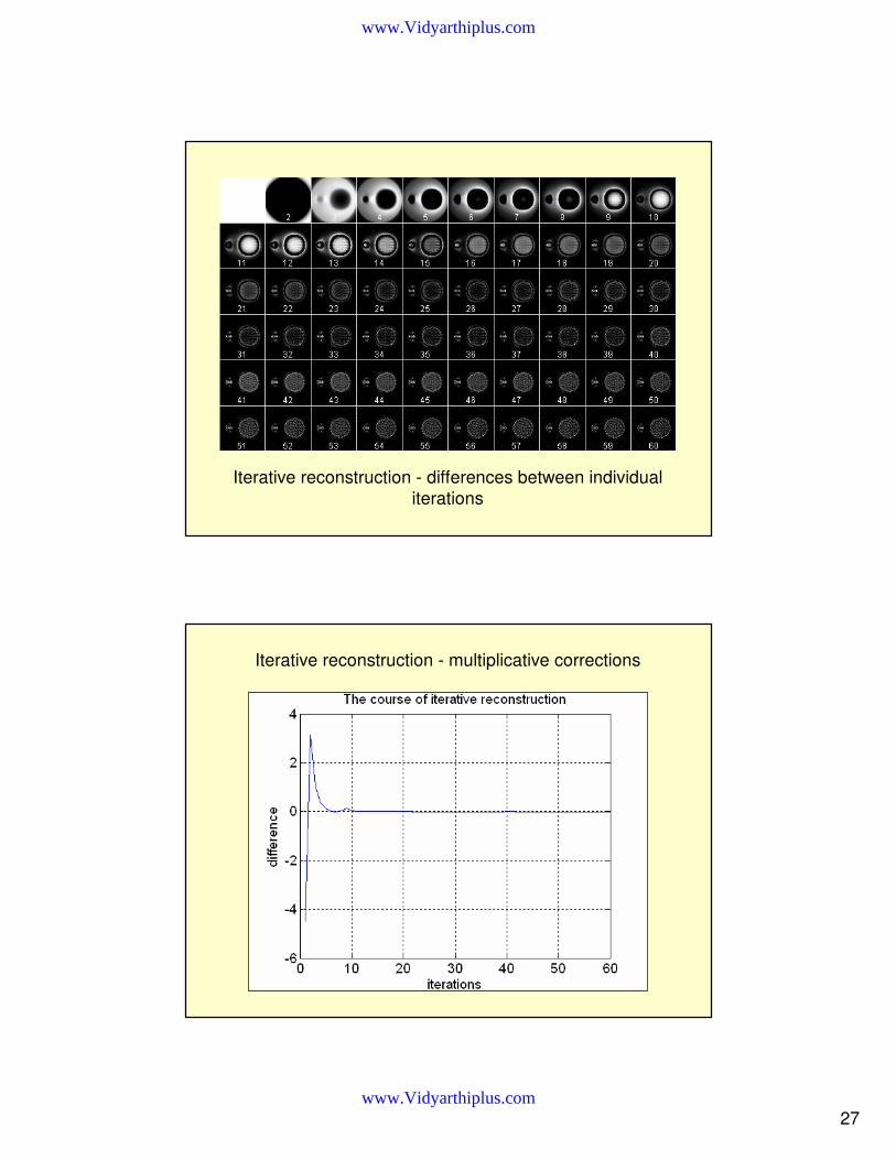
Iterative reconstruction - multiplicative corrections



27

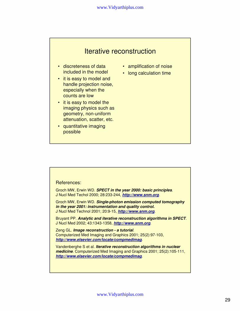
Iterative reconstruction - differences between individual iterations

Iterative reconstruction - multiplicative corrections



28

estimated image differences between subsequent iterations

Sequence of iterations - multiplicative corrections

Filtered back-projection

• very fast• direct inversion of the

projection formula

• corrections for scatter, non-uniform attenuation and other physical factors are difficult

• it needs a lot of filtering -trade-off between blurring and noise

• quantitative imaging difficult



29

Iterative reconstruction

• discreteness of data included in the model

• it is easy to model and handle projection noise, especially when the counts are low

• it is easy to model the imaging physics such as geometry, non-uniform attenuation, scatter, etc.

• quantitative imaging possible

• amplification of noise• long calculation time

References:

Groch MW, Erwin WD. SPECT in the year 2000: basic principles. J Nucl Med Techol 2000; 28:233-244, http://www.snm.org.

Groch MW, Erwin WD. Single-photon emission computed tomography

in the year 2001: instrumentation and quality control.

J Nucl Med Technol 2001; 20:9-15, http://www.snm.org.

Bruyant PP. Analytic and iterative reconstruction algorithms in SPECT. J Nucl Med 2002; 43:1343-1358, http://www.snm.org.

Zeng GL. Image reconstruction - a tutorial. Computerized Med Imaging and Graphics 2001; 25(2):97-103, http://www.elsevier.com/locate/compmedimag.

Vandenberghe S et al. Iterative reconstruction algorithms in nuclear

medicine. Computerized Med Imaging and Graphics 2001; 25(2):105-111, http://www.elsevier.com/locate/compmedimag.



30

References:

Patterson HE, Hutton BF (eds.). Distance Assisted Training Programme

for Nuclear Medicine Technologists. IAEA, Vienna, 2003, http://www.iaea.org.

Busemann-Sokole E. IAEA Quality Control Atlas for Scintillation Camera

Systems. IAEA, Vienna, 2003, ISBN 92-0-101303-5, http://www.iaea.org/worldatom/books, http://www.iaea.org/Publications.

Steves AM. Review of nuclear medicine technology. Society of Nuclear Medicine Inc., Reston, 1996, ISBN 0-032004-45-8, http://www.snm.org.

Steves AM. Preparation for examinations in nuclear medicine

technology. Society of Nuclear Medicine Inc., Reston, 1997, ISBN 0-932004-49-0, http://www.snm.org.

Graham LS (ed.). Nuclear medicine self study program II:

Instrumentation. Society of Nuclear Medicine Inc., Reston, 1996, ISBN 0-932004-44-X, http://www.snm.org.

Saha GB. Physics and radiobiology of nuclear medicine. Springer-Verlag, New York, 1993, ISBN 3-540-94036-7.



Documents

Reconstruction from Projections