Reconstruction and Representation of 3D Objects with Radial BasisFunctions

J. C. Carr1;2 R. K. Beatson2 J. B. Cherrie1 T. J. Mitchell1;2 W. R. Fright1 B. C. McCallum1

T. R. Evans1

1Applied Research Associates NZ Ltd�

2 University of Canterburyy

(a) (b)

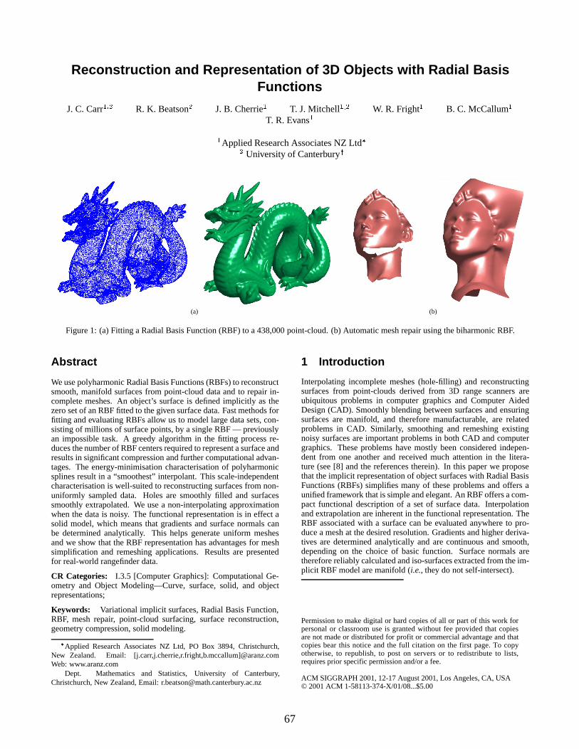
Figure 1: (a) Fitting a Radial Basis Function (RBF) to a 438,000 point-cloud. (b) Automatic mesh repair using the biharmonic RBF.

Abstract

We use polyharmonic Radial Basis Functions (RBFs) to reconstructsmooth, manifold surfaces from point-cloud data and to repair in-complete meshes. An object’s surface is defined implicitly as thezero set of an RBF fitted to the given surface data. Fast methods forfitting and evaluating RBFs allow us to model large data sets, con-sisting of millions of surface points, by a single RBF — previouslyan impossible task. A greedy algorithm in the fitting process re-duces the number of RBF centers required to represent a surface andresults in significant compression and further computational advan-tages. The energy-minimisation characterisation of polyharmonicsplines result in a “smoothest” interpolant. This scale-independentcharacterisation is well-suited to reconstructing surfaces from non-uniformly sampled data. Holes are smoothly filled and surfacessmoothly extrapolated. We use a non-interpolating approximationwhen the data is noisy. The functional representation is in effect asolid model, which means that gradients and surface normals canbe determined analytically. This helps generate uniform meshesand we show that the RBF representation has advantages for meshsimplification and remeshing applications. Results are presentedfor real-world rangefinder data.

CR Categories: I.3.5 [Computer Graphics]: Computational Ge-ometry and Object Modeling—Curve, surface, solid, and objectrepresentations;

Keywords: Variational implicit surfaces, Radial Basis Function,RBF, mesh repair, point-cloud surfacing, surface reconstruction,geometry compression, solid modeling.

�Applied Research Associates NZ Ltd, PO Box 3894, Christchurch,New Zealand. Email: [j.carr,j.cherrie,r.fright,b.mccallum]@aranz.comWeb: www.aranz.com

yDept. Mathematics and Statistics, University of Canterbury,Christchurch, New Zealand, Email: r.beatson@math.canterbury.ac.nz

1 Introduction

Interpolating incomplete meshes (hole-filling) and reconstructingsurfaces from point-clouds derived from 3D range scanners areubiquitous problems in computer graphics and Computer AidedDesign (CAD). Smoothly blending between surfaces and ensuringsurfaces are manifold, and therefore manufacturable, are relatedproblems in CAD. Similarly, smoothing and remeshing existingnoisy surfaces are important problems in both CAD and computergraphics. These problems have mostly been considered indepen-dent from one another and received much attention in the litera-ture (see [8] and the references therein). In this paper we proposethat the implicit representation of object surfaces with Radial BasisFunctions (RBFs) simplifies many of these problems and offers aunified framework that is simple and elegant. An RBF offers a com-pact functional description of a set of surface data. Interpolationand extrapolation are inherent in the functional representation. TheRBF associated with a surface can be evaluated anywhere to pro-duce a mesh at the desired resolution. Gradients and higher deriva-tives are determined analytically and are continuous and smooth,depending on the choice of basic function. Surface normals aretherefore reliably calculated and iso-surfaces extracted from the im-plicit RBF model are manifold (i.e., they do not self-intersect).

Permission to make digital or hard copies of all or part of this work forpersonal or classroom use is granted without fee provided that copiesare not made or distributed for profit or commercial advantage and thatcopies bear this notice and the full citation on the first page. To copyotherwise, to republish, to post on servers or to redistribute to lists,requires prior specific permission and/or a fee.

ACM SIGGRAPH 2001, 12-17 August 2001, Los Angeles, CA, USA© 2001 ACM 1-58113-374-X/01/08...$5.00

67

The benefits of modeling surfaces with RBFs have been recog-nised by Savchenko [19], Carret al. [10] and by Turk &O’Brien [23, 22]. However, this work was restricted to small prob-lems by theO(N2) storage andO(N3) arithmetic operations ofdirect methods. For example, direct fitting of the dragon in Fig. 1(a)would have required 3,000GB just to store the corresponding ma-trix. Consequently, fitting RBFs to real-world scan data has notbeen regarded as computationally feasible for large data sets. Thefast fitting and evaluation methods introduced in this paper meanmodeling surface data from large data sets and complicated objectsis now feasible. In this paper we:

� describe the computational advantages offered by new fastmethods for fitting and evaluating RBFs.

� introduce RBF center reduction for implicit surface model-ing. This results in significant data compression and speedimprovements.

� demonstrate that modeling very large data sets and topologi-cally complicated objects is possible.

� introduce RBF approximation for the problem of reconstruct-ing smooth surfaces from noisy data.

� apply RBFs to the problem of mesh repair (hole-filling) andpoint-cloud surface fitting.

1.1 Implicit surfaces

The surface representation or reconstruction problem can be ex-pressed as

Problem 1.1. Given n distinct points f(xi; yi; zi)gni=1 on a sur-face M in R3 , find a surface M 0 that is a reasonable approximationto M .

Our approach is to model the surface implicitly with a functionf(x; y; z). If a surfaceM consists of all the points(x; y; z) thatsatisfy the equation

f(x; y; z) = 0; (1)

then we say thatf implicitly definesM . Describing surfaces im-plicitly with various functions is a well-known technique [9].

In Constructive Solid Geometry (CSG) an implicit model isformed from simple primitive functions through a combination ofBoolean operations (union, intersection etc) and blending func-tions. CSG techniques are more suited to the design of objects inCAD rather than their reconstruction from sampled data. Piece-wise low-order algebraic surfaces, sometimes referred to as im-plicit patches or semi-algebraic sets, have also been used to definesurfaces implicitly. These are analogous to piecewise parametricsplines except that the surface is implicitly defined by low degreepolynomials over a piecewise tetrahedral domain. An introductionto these techniques and further references can be found in [9].

The distinction between our approach and these well-knowntechniques is that we wish to model the entire object with a singlefunction which is continuous and differentiable. A single functionaldescription has a number of advantages over piecewise parametricsurfaces and implicit patches. It can be evaluated anywhere to pro-duce a particular mesh,i.e., a faceted surface representation canbe computed at the desired resolution when required. Sparse, non-uniformly sampled surfaces can be described in a straightforwardmanner and the surface parameterization problem, associated withpiecewise fitting of cubic spline patches, is avoided.

The representation of objects with single functions has pre-viously been restricted to modeling “blobby” objects such as

molecules [9] and has generally been believed to be infeasible forreal-world objects acquired by 3D scanners. Turk & O’Brien [23]have tried modeling laser scan data with RBFs. However they havebeen restricted to blobby approximations derived from small sub-sets of data consisting of a few hundred to a thousand surface points.More recent work [25] has focussed on simplifying larger data setsto make them computationally manageable. However, the abilityto represent complicated objects of arbitrary topology and modelthe detail obtainable with modern laser scanners, is compromised.Carret al. [10] used RBFs to reconstruct cranial bone surfaces from3D CT scans. Data surrounding large irregular holes in the skullwere interpolated using the thin-plate spline RBF. Titanium platewas then molded into the shape of the fitted surface to form a cranialprosthesis. That paper exploited the interpolation and extrapolationcharacteristics of RBFs as well as the underlying physical proper-ties of the thin-plate spline basic function. However, the approachis restricted to modeling surfaces which can be expressed explicitlyas a function of two variables. In this paper we demonstrate that byusing new fast methods, RBFs can be fitted to 3D data sets consist-ing of millions of points without restrictions on surface topology —the kinds of data sets typical of industrial applications.

Our method involves three steps:

� Constructing a signed-distance function.

� Fitting an RBF to the resulting distance function.

� Iso-surfacing the fitted RBF.

Section 2 of this paper describes how we formulate the surfacefitting problem as a scattered data interpolation problem. Section 3introduces RBFs and Section 4 describes the use of new fast meth-ods which overcome problems that have prevented the use of RBFsin the past. Section 5 introduces RBF center reduction which re-sults in a compact surface representation as well as faster fittingand evaluation times. Section 6 introduces RBF approximation as ameans of smoothing noisy surface data and demonstrates this by re-constructing smooth surfaces from noisy LIDAR (laser rangefinder)data. Section 7 describes iso-surface extraction. Section 8 demon-strates the abilities of RBFs to reconstruct non-trivial surfaces frompoint-clouds and interpolate incomplete meshes. Section 9 drawsconclusions and discusses future work.

surface points

off-surface ‘normal’ points

Figure 2: A signed-distance function is constructed from the sur-face data by specifying off-surface points along surface normals.These points may be specified on either or both sides of the surface,or not at all.

2 Fitting an implicit function to a surface

We wish to find a functionf which implicitly defines a surfaceM0

and satisfies the equation

f(xi; yi; zi) = 0; i = 1; : : : ; n;

68

mm

(a) (b) (c)

Figure 3: Reconstruction of a hand from a cloud of points with and without validation of normal lengths.

wheref(xi; yi; zi)gni=1 are points lying on the surface. In orderto avoid the trivial solution thatf is zero everywhere, off-surfacepoints are appended to the input data and are given non-zero values.This gives a more useful interpolation problem: Findf such that

f(xi; yi; zi) = 0; i = 1; : : : ; n (on-surface points);

f(xi; yi; zi) = di 6= 0; i = n+ 1; : : : ; N (off -surface points):

This still leaves the problem of generating the off-surface pointsf(xi; yi; zi)gNi=n+1 and the corresponding valuesdi.

An obvious choice forf is a signed-distance function, wherethedi are chosen to be the distance to the closest on-surface point.Points outside the object are assigned positive values, while pointsinside are assigned negative values. Similar to Turk & O’Brien [23],these off-surface points are generated by projecting along surfacenormals. Off-surface points may be assigned either side of the sur-face as illustrated in Fig. 2.

Experience has shown that it is better to augment a data pointwith two off-surface points, one either side of the surface. InFig. 3(a) surface points from a laser scan of a hand are shown ingreen. Off-surface points are color coded according to their dis-tance from their associated on-surface point. Hot colors (red) rep-resent positive points outside the surface while cold colors (blue) lieinside. There are two problems to solve; estimating surface normalsand determining the appropriate projection distance.

If we have a partial mesh, then it is straightforward to define off-surface points since normals are implied by the mesh connectivityat each vertex. In the case of unorganised point-cloud data, nor-mals may be estimated from a local neighbourhood of points. Thisrequires estimating both the normal direction and determining thesense of the normal. We locally approximate the point-cloud datawith a plane to estimate the normal direction and use consistencyand/or additional information such as scanner position to resolvethe sense of the normal. In general, it is difficult to robustly es-timate normals everywhere. However, unlike other methods [16]which also rely on forming a signed-distance function, it is not crit-ical to estimate normals everywhere. If normal direction or senseis ambiguous at a particular point then we do not fit to a normal atthat point. Instead, we let the fact that the data point is a zero-point(lies on the surface) tie down the function in that region.

Given a set of surface normals, care must be taken when pro-jecting off-surface points along the normals to ensure that theydo not intersect other parts of the surface. The projected point isconstructed so that the closest surface point is the surface pointthat generated it. Provided this constraint is satisfied, the recon-structed surface is relatively insensitive to the projection distancejdij. Fig. 3(c) illustrates the effect of projecting off-surface pointsinappropriate distances along normals. Off-surface points havebeen chosen to lie a fixed distance from the surface. The result-ing surface, wheref is zero, is distorted in the vicinity of the fin-

gers where opposing normal vectors have intersected and generatedoff-surface points with incorrect distance-to-surface values, both insign and magnitude. In Fig. 3(a) & (b) validation of off-surface dis-tances and dynamic projection has ensured that off-surface pointsproduce a distance field consistent with the surface data. Fig. 4 is across section through the fingers of the hand. The figure illustrateshow the RBF function approximates a distance function near theobject’s surface. The approximately equally spaced iso-contours at+1, 0 and�1 in the top of the figure and the corresponding functionprofile below, illustrate how the off-surface points have generateda function with a gradient magnitude close to 1 near the surface(which corresponds to the zero-crossings in the profile shown).

mm

Figure 4: Cross section through the fingers of a hand reconstructedfrom the point-cloud in Fig. 3. The iso-contours corresponding to+1, 0 and -1 are shown (top) along with a cross sectional profile ofthe RBF (bottom) along the line shown.

3 Radial Basis Function interpolation

Given a set of zero-valued surface points and non-zero off-surfacepoints we now have a scattered data interpolation problem: we wantto approximate the signed-distance functionf(x) by an interpolants(x). The problem can be stated formally as follows,

Problem 3.1. Given a set of distinct nodes X = fxigNi=1 � R3

and a set of function values ffigNi=1 � R, find an interpolant

69

s : R3 ! R such that

s(xi) = fi; i = 1; : : : ; N: (2)

Note that we use the notationx = (x; y; z) for pointsx 2 R3 .The interpolant will be chosen fromBL(2)(R3), the Beppo-Levi

space of distributions onR3 with square integrable second deriva-tives. This space is sufficiently large to have many solutions toProblem 3.1, and therefore we can define the affine space of inter-polants:

S = fs 2 BL(2)(R3) : s(xi) = fi; i = 1; : : : ; Ng: (3)

The spaceBL(2)(R3) is equipped with the rotation invariant semi-norm defined by

ksk2 =

ZR3

�@2s(x)

@x2

�2+

�@2s(x)

@y2

�2+

�@2s(x)

@z2

�2

+ 2

�@2s(x)

@x@y

�2+ 2

�@2s(x)

@x@z

�2

+ 2

�@2s(x)

@y@z

�2dx: (4)

This semi-norm is a measure of the energy or “smoothness” of func-tions: functions with a small semi-norm are smoother than thosewith a large semi-norm. Duchon [12] showed that the smoothestinterpolant,i.e.,

s? = argmins2S

ksk;

has the simple form

s?(x) = p(x) +NXi=1

�ijx� xij; (5)

wherep is a linear polynomial, the coefficients�i are real numbersandj � j is the Euclidean norm onR3 .

This function is a particular example of aradial basis function(RBF). In general, an RBF is a function of the form

s(x) = p(x) +

NXi=1

�i�(jx� xij); (6)

wherep is a polynomial of low degree and thebasic function � isa real valued function on[0;1), usually unbounded and of non-compact support (see,e.g., Cheney & Light [11]). In this contextthe pointsxi are referred to as thecenters of the RBF.

Popular choices for the basic function� include the thin-platespline�(r) = r2 log(r) (for fitting smooth functions of two vari-ables), the Gaussian�(r) = exp(�cr2) (mainly for neural net-works), and the multiquadric�(r) =

pr2 + c2 (for various ap-

plications, in particular fitting to topographical data). For fittingfunctions of three variables, good choices include the biharmonic(�(r) = r, i.e., Equation (5)) and triharmonic (�(r) = r3) splines.

RBFs are popular for interpolating scattered data as the associ-ated system of linear equations is guaranteed to be invertible undervery mild conditions on the locations of the data points [11, 18].For example, the biharmonic spline of Equation (5) only requiresthat the data points are not co-planar, while the Gaussian and mul-tiquadric place no restrictions on the locations of the points. In par-ticular, RBFs do not require that the data lie on any sort of regulargrid.

An arbitrary choice of coefficients�i in Equation (5) will yielda functions? that is not a member ofBL(2)(R3). The requirementthats? 2 BL(2)(R3) implies the orthogonality or side conditions

NXi=1

�i =NXi=1

�ixi =NXi=1

�iyi =NXi=1

�izi = 0:

More generally, if the polynomial in Equation (6) is of degreemthen the side conditions imposed on the coefficients are

NXi=1

�iq(xi) = 0; for all polynomialsq of degree at mostm: (7)

These side conditions along with the interpolation conditions ofEquation (2) lead to a linear system to solve for the coefficientsthat specify the RBF.

Let fp1; : : : ; p`g be a basis for polynomials of degree at mostm and letc = (c1; : : : ; c`) be the coefficients that givep in termsof this basis. Then Equations (2) and (7) may be written in matrixform as �

A PP T 0

���c

�= B

��c

�=

�f0

�; (8)

where

Ai;j = �(jxi � xj j); i; j = 1; : : : ; N;

Pi;j = pj(xi); i = 1; : : : ; N; j = 1; : : : ; `:

In the specific case of the biharmonic spline in 3D, if it is assumedthat the polynomial part of the RBF in Equation (5) has the formp(x) = c1 + c2x+ c3y + c4z, then

Ai;j = jxi � xj j; i; j = 1; : : : ; N;

P is the matrix withith row(1; xi; yi; zi),� = (�1; : : : ; �N)T andc = (c1; c2; c3; c4)

T.Solving the linear system (8) determines� and c, and hence

s(x). However, the matrixB in Equation (8) typically has poorconditioning as the number of data pointsN gets larger. This meansthat substantial errors will easily creep into any standard numericalsolution.

On initial inspection, the essentially local nature of the Gaussian,inverse multiquadric (�(r) = (r2 + c2)�1=2) and compactly sup-ported basic functions appear to lead to more desirable properties inthe RBF. For example, the matrix B now has special structure (spar-sity) which can be exploited by well-known methods and evaluationof Equation (6) only requires that the sum be over nearby centersinstead of allN centers. However, non-compactly supported ba-sic functions are better suited to extrapolation and interpolation ofirregular, non-uniformly sampled data. Indeed, numerical experi-ments using Gaussian and compactly supported piecewise polyno-mials for fitting surfaces to point-clouds have shown that these basicfunctions yield surfaces with many undesirable artifacts in additionto the lack of extrapolation across holes.

The energy minimisation properties of biharmonic splines makethem well suited to the representation of 3D objects. Since the cor-responding basic function�(r) = r is not compactly supportedand grows arbitrarily large asr tends to infinity, the correspond-ing matrixB of Equation (8) is not sparse and, except for sym-metry, has no obvious structure that can be exploited in solvingthe system. Storing the lower triangle of matrixB requires spacefor N(N + 1)=2 real numbers. Solution via a symmetric solverwill require N3=6 + O(N2) flops. For a problem with20; 000data points this is a requirement for approximately1:6� 109 bytes(1.5GB) of core memory, and1013 flops, which is impractical. Fur-thermore, ill-conditioning of the matrixB is likely to make anysolution one gets from such a direct computation highly unreliable.Thus, it is clear that direct methods are inappropriate for problemswith N & 2; 000. Moreover, a single direct evaluation of Equa-tion (6) requiresO(N) operations. These factors have led manyauthors to conclude that, although RBFs are often the interpolantof choice, they are only suitable for problems with at most a fewthousand points [13, 14, 20]. The fast methods described in thefollowing section demonstrate that this is no longer the case.

70

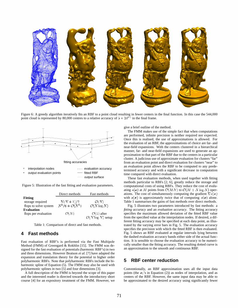
Figure 6: A greedy algorithm iteratively fits an RBF to a point cloud resulting in fewer centers in the final function. In this case the 544,000point cloud is represented by 80,000 centres to a relative accuracy of5� 10�4 in the final frame.

output surface

evaluation accuracyfitted RBF

fitting accuracies

output evaluation pointsinterpolation nodes

Figure 5: Illustration of the fast fitting and evaluation parameters.

Direct methods Fast methodsFittingstorage required N(N + 1)=2 O(N)flops to solve system N3=6 +O(N2) O(N logN)Evaluationflops per evaluation O(N) O(1) after

O(N logN) setup

Table 1: Comparison of direct and fast methods.

4 Fast methods

Fast evaluation of RBF’s is performed via the Fast MultipoleMethod (FMM) of Greengard & Rokhlin [15]. The FMM was de-signed for the fast evaluation of potentials (harmonic RBF’s) in twoand three dimensions. However Beatsonet al. [7] have adapted theexpansion and translation theory for the potential to higher orderpolyharmonic RBFs. Note that polyharmonic RBFs include the bi-harmonic spline of Equation (5). The FMM may also be used withpolyharmonic splines in two [5] and four dimensions [3].

A full description of the FMM is beyond the scope of this paperand the interested reader is directed towards the introductory shortcourse [4] for an expository treatment of the FMM. However, we

give a brief outline of the method.The FMM makes use of the simple fact that when computations

are performed, infinite precision is neither required nor expected.Once this is realised, the use of approximations is allowed. Forthe evaluation of an RBF, the approximations of choice are far- andnear-field expansions. With the centers clustered in a hierarchicalmanner, far- and near-field expansions are used to generate an ap-proximation to that part of the RBF due to the centers in a particularcluster. A judicious use of approximate evaluation for clusters “far”from an evaluation point and direct evaluation for clusters “near” toan evaluation point allows the RBF to be computed to any prede-termined accuracy and with a significant decrease in computationtime compared with direct evaluation.

These fast evaluation methods, when used together with fittingmethods particular to RBFs [2, 6], greatly reduce the storage andcomputational costs of using RBFs. They reduce the cost of evalu-atings(x) atM points fromO(MN) toO(M + N logN) oper-ations. The cost of simultaneously computing the gradientrs(x)with s(x) is approximately twice that of computings(x) alone.Table 1 summarises the gains of fast methods over direct methods.

Fig. 5 illustrates two parameters introduced by fast methods: afitting accuracy and anevaluation accuracy. The fitting accuracyspecifies the maximum allowed deviation of the fitted RBF valuefrom the specified value at the interpolation nodes. If desired, a dif-ferent fitting accuracy may be specified at each data point, as illus-trated by the varying error bars in Fig. 5. The evaluation accuracyspecifies the precision with which the fitted RBF is then evaluated.Fig. 5 shows an RBF evaluated at regular intervals lying betweenthe dashed evaluation accuracy bands either side of the actual func-tion. It is sensible to choose the evaluation accuracy to be numeri-cally smaller than the fitting accuracy. The resulting dotted curve isan approximation to the smooth and continuous RBF.

5 RBF center reduction

Conventionally, an RBF approximation uses all the input datapoints (thexi ’s in Equation (2)) as nodes of interpolation, and ascenters of the RBF. However, the same input data may be able tobe approximated to the desired accuracy using significantly fewer

71

RBF centers reduced subsetof RBF centers

Figure 7: Illustration of center reduction.

centers, as illustrated in Fig. 7. A greedy algorithm can therefore beused to iteratively fit an RBF to within the desiredfitting accuracy.

A simple greedy algorithm consists of the following steps:

1. Choose a subset from the interpolation nodesxi and fit anRBF only to these.

2. Evaluate the residual,�i = fi � s(xi), at all nodes.

3. If maxfj�ijg < fitting accuracy then stop.

4. Else append new centers where�i is large.

5. Re-fit RBF and goto 2.

If a different accuracyÆi is specified at each point, then the condi-tion in step 3 may be replaced byj�ij < Æi.

Center reduction is not essential when using the fast methodsdescribed in Section 4. For example, no reduction was used whenfitting to the LIDAR example of Fig. 8. However, reducing thenumber of RBF centers results in smaller memory requirements andfaster evaluation times, without a loss in accuracy. Fig. 6 illustratesthe fitting process with center reduction. As more centers are addedto the RBF, the zero-surface more closely approximates the entireset of data points. In this case, a laser scan of a Buddha figurine,consisting of 544,000 points, has been approximated by an RBFwith 80,000 centers to a relative accuracy of1:4� 10�4 (achievedat all the data points).

The greedy algorithm often results in a net faster fitting time,even with a moderate reduction in the number of centers. Thisis due to the efficiencies associated with solving and evaluating asimilar system at each iteration and the fact that initial iterationsinvolve solving much smaller problems. The results presented inSection 8 are typical of our experience and show that dense laserscan data can be represented by significantly fewer centers than thetotal number of data points.

6 RBF approximation of noisy data

In Section 3 we looked for an interpolant that minimized a measureof smoothness. However, if there is noise in the data, the interpola-tion conditions of Equation (2) are too strict and we would prefer toplace more emphasis on finding a smooth function, where smooth-ness is measured by Equation (4). Thus, consider the problem

mins2BL(2)(R3)

�ksk2 + 1

N

NXi=1

�s(xi)� fi

�2; (9)

where� � 0 and k � k is defined in Equation (4). The param-eter� balances smoothness against fidelity to the data. It can beshown [24] that the solutions? to this problem also has the form of

Equation (5), but now the coefficient vector(�T; cT)T is the solu-tion to

�A� 8N��I P

P T 0

���c

�=

�f0

�; (10)

where the matricesA andP are as in Equation (8). The parameter�can be thought of as the stiffness of the RBFs(x). The system (10)can also be solved using fast methods.

In Fig. 8 we illustrate RBF approximation (also known as splinesmoothing) in the context of reconstructing a surface from 3D LI-DAR data. LIDAR data is often noisy and irregular due to limitedrange resolution and misregistration between scans taken at differ-ent scanner positions. Restricted physical viewing angles for thescanner mean increased susceptibility to occlusion and therefore re-gions of incomplete data. Elsewhere, due to overlapping scans, thedata may contain redundancy. Consequently, LIDAR scans repre-sent one of the more difficult surface fitting problems. In this exam-ple a smooth surface has been automatically fitted to LIDAR scansof a fountain in Santa Barbara using an RBF approximation. Thestatue is approximately 2m�5m and was scanned using a CYRAX2400 scanner. The data set consists of 350,000 points imaged fromseveral viewpoints in front of the statue. Three spheres apparent ontop of and beside the statue correspond to landmarks added to thescene in order to align the scans. Fig. 8(a) is the point-cloud takenfrom several scanner positions in front of the statue. Note the largeoccluded regions where no data has been recorded. Fig. 8(b) is theautomatically fitted RBF surface. Fig. 8(c) is a detailed view of thefitted surface which illustrates how the smoothness constraint inher-ent in the biharmonic RBF has correctly preserved the gap betweenthe arm and the rest of the statue, despite having no data in theseregions. Along the cut-away planes in this figure we show the mag-nitude of the RBF. Lighter colored points have smaller magnitudes,i.e., they are “closer” to the zero-surface than darker points.

Fig. 9 illustrates the affect of varying� on a detailed portion ofthe surface in Fig. 8. Fig. 9(a) is an exact fit to the raw data (� = 0),Fig. 9(b) is the value of� corresponding to Fig. 8(b) and Fig. 9(c)illustrates increased smoothing with a larger value for�.

In this example a global value for� has been chosen, however,by dividing Equation (9) by� it is possible to specify a particularsmoothing parameter�i for each data point or group of points.

7 Surface evaluation

An RBF fitted to a set of surface data forms asolid model of an ob-ject. The surface of the object is the locus of points where the RBFis zero. This surface can be visualised directly using an implicitray-tracer [9], or an intermediate explicit representation, such as amesh of polygons, can be extracted. In the latter case, well-knowniso-surfacing algorithms such as Marching Cubes [17] can be usedto polygonize the surface. However, conventional implementationsare optimised for visualising a complete volume of data sampled ona regular voxel grid. The cost associated with evaluating an RBFmeans that an efficient surface-following algorithm is desirable.

In this paper a marching tetrahedra variant, optimised for surfacefollowing, has been used to polygonize surfaces. A mesh optimisa-tion scheme adapted from [21] results in fewer triangles with betteraspect ratios,i.e., thin and elongated triangles are avoided. A typ-ical output mesh from this algorithm is illustrated in Fig. 10(b).Wavefronts of facets spread out from seed points across the surfaceuntil they meet or intersect the bounding box. For clarity, awave-front from a single seed is shown in red in Fig. 10(a) spreading overthe surface of the Buddha figurine during iso-surfacing. Surface-following is initiated from seed points corresponding to RBF cen-ters. By design, many centers will lie on, or very near, the surface.In the case of off-surface centers, the RBF gradient is used to search

72

(a) (b) (c)

Figure 8: RBF approximation of noisy LIDAR data. (a) 350,000 point-cloud, (b) the smooth RBF surface approximates the original point-cloud data, (c) cut-away view illustrating the RBF distance field and the preservation of the gap between the arm and the torso.

(a) (b) (c)

Figure 9: (a) Exact fit, (b) medium amount of smoothing applied (the RBF approximates at data points), (c) increased smoothing.

for the nearest zero-crossing. Convergence is rapid because thegradient is approximately constant near the surface. Local minimahave not been observed in our experience, but this is not surprisingsince we deliberately constructed the function in Section 2 to havethese properties. In any case, only a small subset of centers is re-quired to seed the surface, one for each distinct surface section. Thesurface-following strategy avoids the conventional requirement fora 3D array of sample points and therefore minimises the number ofRBF evaluations. Consequently, the computational cost increaseswith the square of the resolution, rather than the cube, as it would ifa complete volume were sampled. Memory overhead is also min-imised since it is only necessary to retain the sample vertices as-sociated with the advancingwavefronts. Quadrilateral meshes canalso be produced in this manner. Surfacing ambiguities can be re-solved easily due to the ability to analytically evaluate the gradientof the RBF.

8 Results

Table 2 quantifies the fitting and evaluation times for the figurespresented in this paper. In all cases the biharmonic spline was fit-

ted. Two off-surface points were generated for every second pointin the original surface data, hence the number of interpolation nodesto which an RBF is fitted is approximately twice the number of sur-face points. Center reduction was used throughout, except in theLIDAR example, where the number of RBF centers consequentlyequals the number of interpolation nodes. Fitting and evaluationwas performed on a 550MHz PIII Pentium with 512MB RAM.Figs. 1(a), 3, 6, 12, 13 and 14 illustrate fitting surfaces to point-clouds while Figs. 1(b) and 11 illustrate fitting to partial meshes.Fig. 8 demonstrates approximation with an RBF in the context offitting a smooth surface to noisy LIDAR data.

The dragon in Fig. 1(a), the Buddha figurine (Fig. 6) and theskeleton hand (Fig. 12) demonstrate the ability of fast methods tomodel large complicated data sets to high accuracy and the com-pact nature of the RBF representation. The dragon data was derivedfrom a mesh consisting of 438,000 vertices and 871,000 faces, theBuddha from 544,000 vertices and 1,087,000 faces. Normals werecomputed at vertices from the adjacent faces. Direct methods wouldinevitably fail on these problems. For example, a direct approachto fitting the Buddha data would require 4,700GB of storage justto store the matrix of the interpolation system (8). The peak corememory requirements of the new fast methods in Table 2 are par-

73

(a) (b)

Figure 10: Iso-surfacing an RBF. (a) Surface-following from a single seed, (b) example of an optimised mesh.

Figure Number of Number of inter- Number of Peak RAM Fitting Surfacing Relativesurface points -polation nodes RBF centers (MB) time time accuracy

Face 14,806 29,074 3,564 29 68s 27s 7�10�4Hand 13,348 26,696 4,299 29 97s 32s 1�10�3

Dragon 437,645 872,487 72,461 306 2:51:09 0:04:40 8�10�4Buddha 543,652 1,086,194 80,518 291 4:03:26 0:04:07 5�10�4

Cherub statue 331,135 662,269 83,293 187 3:09:06 0:06:41 4�10�4Skeleton hand 327,323 654,645 85,468 188 3:08:44 0:04:04 3�10�4LIDAR statue 345,910 518,864 518,864 390 3:08:21 0:25:39 6�10�3

Table 2: Comparison of RBF fitting and evaluation times on a 550MHz PIII with 512MB RAM.

ticularly noteworthy in this respect.Fig. 1(b) and Fig. 11 illustrate the application of RBFs to mesh

repair. In Fig. 1(b) an RBF is fitted to a partial mesh obtained from alaser scanner. This figure demonstrates the ability of the biharmonicspline to smoothly interpolate across large irregular holes, for ex-ample under the chin, and smoothly extrapolate a surface far fromthe data. In Fig. 11 an RBF has been fitted to a large statue dataset. Although carefully scanned, the statue contains many smallholes and larger holes corresponding to occluded regions betweenthe embracing figures. The fitted RBF has automatically filled allthe holes and generated a water-tight model of the statue withoutthe user having to specify any parameters other than the desired fit-ting accuracy. Note how the fragment of shoulder data on the rightfigurine has been extrapolated to reconstruct the missing chest data.

Fig. 13 illustrates the reconstruction of the asteroid Eros fromscattered range data. This is a good example of non-uniformlydistributed data, often difficult to reconstruct using other methods.Furthermore, in this example the accuracy associated with the rangemeasurements varies at each point.

Table 3 compares the size of the original meshes in the dragon,Buddha and skeletal hand data sets with the size of the equivalentRBF representation. The uncompressed mesh sizes were derivedby assigning 3 floats (12 bytes) to each vertex and 3 integers (12bytes) to each triangular facet. The uncompressed RBF file sizecorresponds to representing each center with 3 floats (12 bytes) andeach coefficient (�i) with a double precision number (8 bytes). It islikely that single precision would be adequate, which would resultin more compression, but we have not yet quantified the effect ofcoefficient precision on the evaluated surface. This table demon-strates the significant compression of both point-cloud and meshdata that an RBF representation offers. We have also listed the size

of the meshes derived from evaluating the RBF at a comparableresolution to the original data. It appears from initial results that apromising application of RBFs is the remeshing of existing meshes.Fitting an RBF not only fills holes, but a more uniform (and hencemore compact) mesh can be derived from it.

Finally, for the doubting reader, we demonstrate in Figure 14 thata single RBF can model an extremely complicated surface with ahigh genus. In this case 594,000 centers were required to modelthe turbine blade to10�4 accuracy. The fast evaluation methodsdescribed in Section 4 are essential for working with RBFs of thissize. The RBF has reproduced intricate internal structure along withsurface detail present in the original data. The point-cloud datawere only available as a Marching Cubes (MC) mesh derived fromX-ray CT data. However, if the CT data were available, then wewould fit an RBF directly to the CT values. Specifically, we wouldfit to a subset of the data with values in the vicinity of the thresholdused by Marching Cubes to iso-surface the data. This would resultin a smaller fitting problem since the MC mesh contains extraneousvertices and the construction of a signed-distance function, whichrequires adding off-surface points, would be avoided. Smooth RBFinterpolation of the CT data would also be preferable to the linearinterpolation used in the MC algorithm, particularly between CTslices, which are usually spaced further apart relative to the pixelresolution within a slice. An approximating spline could also beused to reduce noise in the CT data.

9 Summary and future work

Fast methods make it computationally possible to represent com-plicated objects of arbitrary topology by RBFs. The scale-

74

Original mesh New mesh RBF representationFigure # vertices # facets Storage # vertices # facets StorageRBF centers StorageDragon 437,645 847,414 15.4MB 126,998 254,016 4.5MB 72,461 1.4MBBuddha 543,652 1,086,798 19.6MB 96,766 193,604 3.5MB 80,518 1.6MB

Skeleton hand 327,323 654,666 11.8MB 81,829 163,698 2.9MB 85,468 1.7MB

Table 3: Comparison of storage requirements for RBF representations and derived meshes.

Figure 11: An RBF has automatically filled small holes and extrap-olated across occluded regions in the scan data (left), to producea closed, water-tight model (right). The complex topology of thestatue has been preserved.

Figure 12: With sufficient sampling, complicated objects can berepresented with RBFs.

independent, “smoothest interpolator” characterisation of polyhar-monic splines make RBFs particularly suited to fitting surfaces tonon-uniformly sampled point-clouds and partial meshes that con-tain large irregular holes. The smoothest surface, most consistentwith the input data, is produced. Details are resolved, provided theyare adequately sampled. The functional nature of the RBF represen-tation offers new possibilities for surface registration algorithms,mesh simplification, compression and smoothing algorithms.

Within a Constructive Solid Geometry (CSG) framework theRBF offers a new way of modeling real-world (scanned) objectssince it is inherently a solid model. It can be manipulated througha series of Boolean unions and intersections with other objects ina manner similar to how simpler geometric primitives are currentlyused to construct more complicated objects.

RBFs are also relevant to the problem of visualising volume data

Figure 13: RBF reconstruction of the asteroid Eros from non-uniformly distributed range data (top). Photograph and model froma similar view (bottom).

acquired on an irregular grid, as can occur in medical imaging andgeophysical data. Here an RBF can be fitted to the sampled datain order to approximate the underlying scalar distribution. Vectorfields can be modeled easily if the components are independent.In that case, an RBF can be fitted to each field component. Thisdoes not require much extra computation time since the matrix inEquation (8) depends only on the location of the interpolation nodesand is therefore common to each component RBF.

Planned future work includes improving the performance ofthe reduction algorithm presented in Section 5. We have alreadyachieved better reductions in the number of centers than those givenin Table 2 but at the cost of slower fitting times. For example, thedragon has been modeled by as few as 32,000 centers and the Bud-dha by 42,000 centers, to the same fitting accuracy. This improve-ment was achieved by simply adding fewer centers to the RBF ateach iteration. The global nature of the RBF representation impliesRBFs inherit the drawbacks of any global model when manipula-tion of part of that model or ray-tracing is required. However, webelieve that it should be straightforward to decompose a global RBFdescription into a piecewise mesh of implicit surface patches in thespirit of [1] to facilitate local manipulation and ray-tracing. Futurespeed improvements in computing and evaluating RBFs are likelyto come from the inherent suitability of the algorithms to parallelprocessing and by tailoring to particular applications. In particular,we believe that significant speed improvements are likely if the datalie on a grid, albeit an incompletely sampled grid.

75

Figure 14: Solid and semi-transparent renderings of an RBF model of a turbine blade containing intricate internal structure. The RBF has594,000 centers.

10 Acknowledgements

This research has been supported by FRST contracts DRFX-9902,DRFX-0001 and ARA-801. We are grateful to Stanford ComputerGraphics Laboratory for the Buddha and Dragon data, to CornellUniversity and NASA for the Eros data, to Georgia Institute ofTechnology and the Large Geometric Models Archive for the tur-bine and skeleton data, to Allen Instruments and Supplies, USA,for the LIDAR data and PolhemusFastSCAN for all other data.

References[1] C. Bajaj, J. Chen, and G. Xu. Modeling with cubic a-patches.ACM Transactions

on Computer Graphics, 14(2):103–133, 1995.

[2] R. K. Beatson, J. B. Cherrie, and C. T. Mouat. Fast fitting of radial basis func-tions: Methods based on preconditioned GMRES iteration.Advances in Compu-tational Mathematics, 11:253–270, 1999.

[3] R. K. Beatson, J. B. Cherrie, and D. L. Ragozin. Fast evaluation of radial basisfunctions: Methods for four-dimensional polyharmonic splines.SIAM J. Math.Anal., 32(6):1272–1310, 2001.

[4] R. K. Beatson and L. Greengard. A short course on fast multipole methods.In M. Ainsworth, J. Levesley, W.A. Light, and M. Marletta, editors,Wavelets,Multilevel Methods and Elliptic PDEs, pages 1–37. Oxford University Press,1997.

[5] R. K. Beatson and W. A. Light. Fast evaluation of radial basis functions: Methodsfor two-dimensional polyharmonic splines.IMA Journal of Numerical Analysis,17:343–372, 1997.

[6] R. K. Beatson, W. A. Light, and S. Billings. Fast solution of the radial basisfunction interpolation equations: Domain decomposition methods.SIAM J. Sci.Comput., 22(5):1717–1740, 2000.

[7] R. K. Beatson, A. M. Tan, and M. J. D. Powell. Fast evaluation of radial basisfunctions: Methods for 3-dimensional polyharmonic splines. In preparation.

[8] F. Bernardini, C. L. Bajaj, J. Chen, and D. R. Schikore. Automatic reconstructionof 3D CAD models from digital scans.Int. J. on Comp. Geom. and Appl., 9(4–5):327, Aug & Oct 1999.

[9] J. Bloomenthal, editor.Introduction to Implicit Surfaces. Morgan Kaufmann,San Francisco, California, 1997.

[10] J. C. Carr, W. R. Fright, and R. K. Beatson. Surface interpolation with radialbasis functions for medical imaging.IEEE Trans. Medical Imaging, 16(1):96–107, February 1997.

[11] E. W. Cheney and W. A. Light.A Course in Approximation Theory. BrooksCole, Pacific Grove, 1999.

[12] J. Duchon. Splines minimizing rotation-invariant semi-norms in Sobolev spaces.In W. Schempp and K. Zeller, editors,Constructive Theory of Functions of Sev-eral Variables, number 571 in Lecture Notes in Mathematics, pages 85–100,Berlin, 1977. Springer-Verlag.

[13] N. Dyn, D. Levin, and S. Rippa. Numerical procedures for surface fitting ofscattered data by radial functions.SIAM J. Sci. Stat. Comput., 7(2):639–659,1986.

[14] J. Flusser. An adaptive method for image registration.Pattern Recognition,25(1):45–54, 1992.

[15] L. Greengard and V. Rokhlin. A fast algorithm for particle simulations.J. Com-put. Phys, 73:325–348, 1987.

[16] H. Hoppe, T. DeRose, T. Duchamp, J. McDonald, and W. Stuetzle. Surface re-constuction from unorganized points.Computer Graphics (SIGGRAPH’92 pro-ceedings), 26(2):71–78, July 1992.

[17] W. E. Lorensen and H. E. Cline. Marching cubes: A high resolution 3D surfaceconstruction algorithm.Computer Graphics, 21(4):163–169, July 1987.

[18] C. A. Micchelli. Interpolation of scattered data: Distance matrices and condi-tionally positive definite functions.Constr. Approx., 2:11–22, 1986.

[19] V. V. Savchenko, A. A. Pasko, O. G. Okunev, and T. L. Kunii. Function rep-resentation of solids reconstructed from scattered surface points and contours.Computer Graphics Forum, 14(4):181–188, 1995.

[20] R. Sibson and G. Stone. Computation of thin-plate splines.SIAM J. Sci. Stat.Comput., 12(6):1304–1313, 1991.

[21] G. M. Treece, R. W. Prager, and A. H. Gee. Regularised marching tetrahedra: im-proved iso-surface extraction.Computers and Graphics, 23(4):583–598, 1999.

[22] G. Turk and J. F. O’Brien. Shape transformation using variational implicit sur-faces. InSIGGRAPH’99, pages 335–342, Aug 1999.

[23] G. Turk and J. F. O’Brien. Variational implicit surfaces. Technical Report GIT-GVU-99-15, Georgia Institute of Technology, May 1999.

[24] G. Wahba.Spline Models for Observational Data. Number 59 in CBMS-NSFRegional Conference Series in Applied Math. SIAM, 1990.

[25] G. Yngve and G. Turk. Creating smooth implicit surfaces from polygonalmeshes. Technical Report GIT-GVU-99-42, Georgia Institute of Technology,1999.

76