Sandia is a multiprogram laboratory operated by Sandia Corporation, a Lockheed Martin Company,for the United States Department of Energy under contract DE-AC04-94AL85000.

Reconnect ‘04Solving Integer Programs with Branch and

Bound (and Branch and Cut)

Cynthia Phillips (Sandia National Laboratories)

Slide 2

One more general branch and bound point

Node selection: when working in serial, how do you pick an active node

to process next?

Usual: best first

• Select the node with the lowest lower bound

• With the current incumbent and solution tolerances, you will have to

evaluate it anyway

If you don’t have a good incumbent finder, you might start with diving:

• Select the most refined node

• Once you have an incumbent, switch to best first

Slide 3

Mixed-Integer programming (IP)

Min

Subject to:

cTx

€

€

Ax = b

l ≤ x ≤ u

x = (xI , xC )

xI ∈ Z n (integer values)

xC ∈ Qn (rational values)

Slide 4

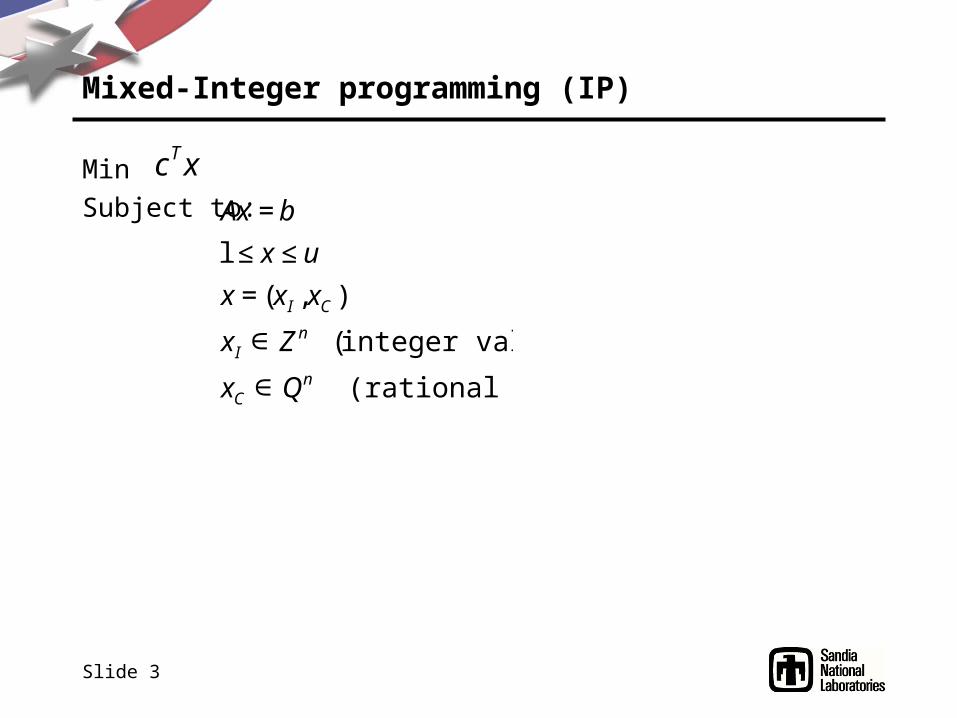
Branch and Bound

• Bounding function: solve LP relaxation

• Branching

– Select an integer variable xi that’s fractional in the LP solution x*

– Up child: set

– Down child: set

– x* is no longer feasible in either child

• Incumbent method

– many incumbent-finding methods to follow in later lectures

– Obvious: return the LP solution if it is integer

• Satisfies feasibility-tester constraint

€

x i ≤ x i*

⎣ ⎦

€

x i ≥ x i*⎡ ⎤

Slide 5

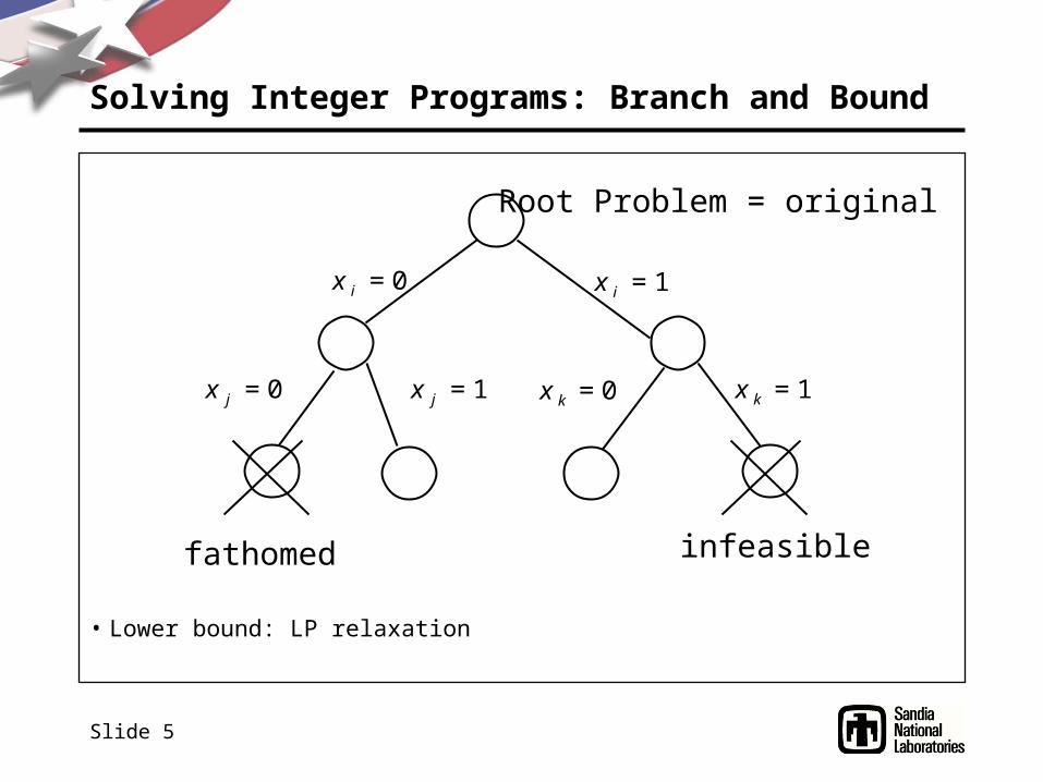
Solving Integer Programs: Branch and Bound

• Lower bound: LP relaxation

x k = 0 x k = 1

x i = 1

x j = 1 x j = 0

x i = 0

Root Problem = original

fathomed infeasible

Slide 6

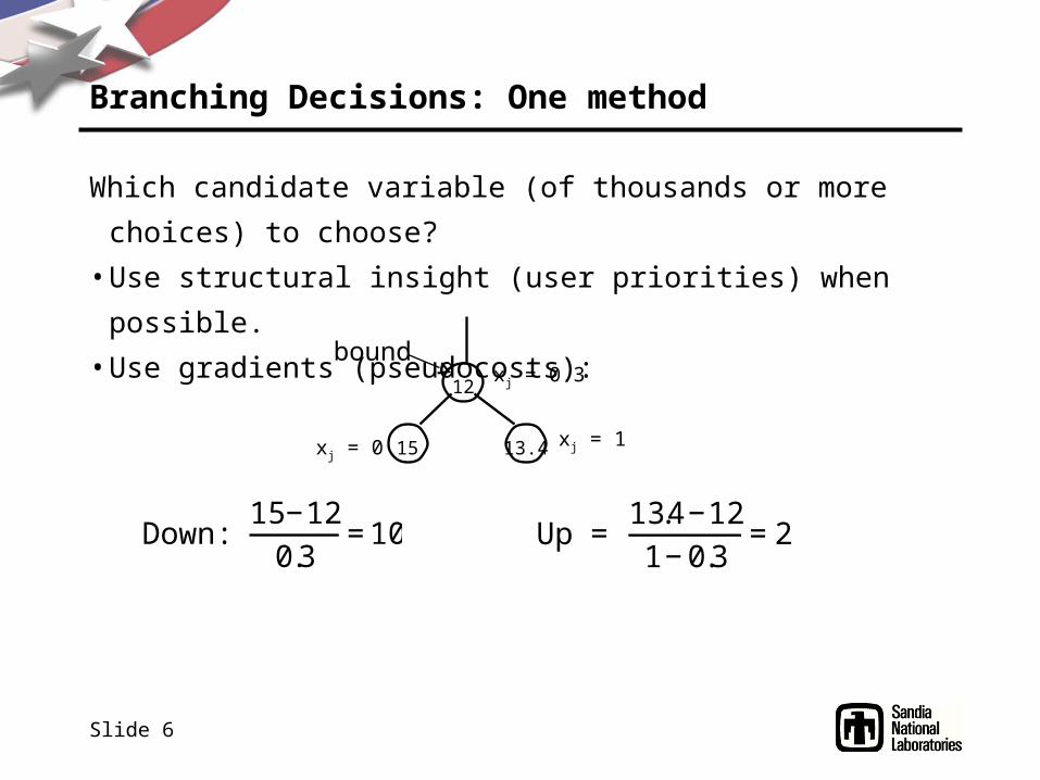
Branching Decisions: One method

Which candidate variable (of thousands or more choices) to choose?

• Use structural insight (user priorities) when possible.

• Use gradients (pseudocosts):

12

13.415

xj = 0.3

xj = 1xj = 0

Down: 15−12

0.3=10 Up =

13.4−121−0.3

=2

bound

Slide 7

Using gradients

• Use gradients to compute an expected bound movement for each child

– Up = up gradient * upward round distance

– Down = down gradient * downward round distance

• Try to find a variable for which both children might move the bound

Initialization

• When a variable is fractional for the first time, intialize by “pretending”

to branch (better than using an average)

Slide 8

Branch Variable Selection method 2: Strong Branching

• “Try out” interesting subproblems for a while

– Could be like a gradient “initialization” at every node

– Could compute part of the subtree

• This can be expensive, but sometimes these decisions make a huge

difference (especially very early)

Slide 9

Branching on constraints

Can have one child with new constraint:

and the other with new constraint:

• Must cover the subregion

• Pieces can be omitted, but only if provably have nothing potentially

optimal

• Node bounds are just a special case

More generally, partition into many children

€

aT x ≤ b1

€

aT x ≥ b2

€

aT x ≤ b1, b2 ≤ aT x ≤ b3, K , bk−1 ≤ x ≤ bk

Slide 10

Special Ordered Sets (SOS)

• Models selection:

Example: time-indexed scheduling

• xjt = 1 if job j is scheduled at time t

• Ordered by time

€

y ii=1

m

∑ =1

y i ∈ 0,1{ }

Slide 11

Special Ordered Sets: Restricted Set of Values (Review)

• Variable x can take on only values in

– Frequently the vi are sorted

• Capacity of an airplane assigned to a flight

– The yi’s are a special ordered set.

€

v1,v2,K vm{ }

€

x = v i

i=1

m

∑ y i

y ii=1

m

∑ =1

y ∈ 0,1{ }

Slide 12

Problems with Simple Branching on SOS

Generally want both children to differ from parent substantially

For SOS

• The up child (setting a variable to 1) is very powerful

– All others in the set go to zero

• The down child will likely have an LP solution = parent’s

– “Schedule at any of these 1000 times except this one”

Slide 13

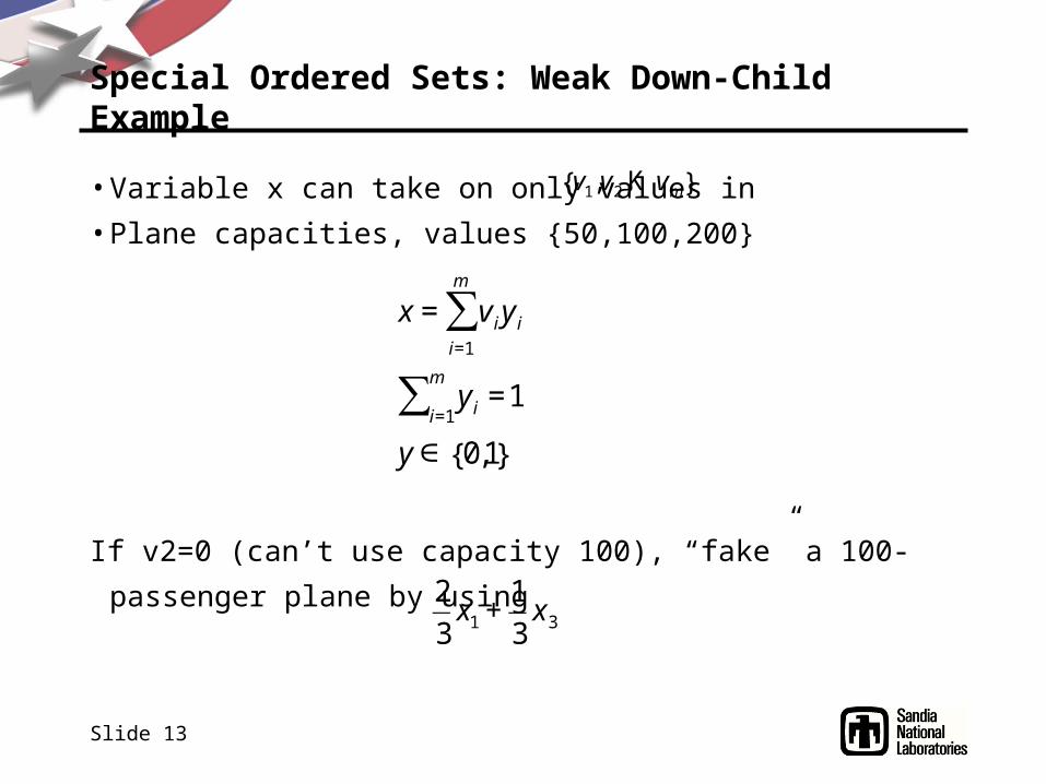
Special Ordered Sets: Weak Down-Child Example

• Variable x can take on only values in

• Plane capacities, values {50,100,200}

If v2=0 (can’t use capacity 100), “fake” a 100-passenger plane by using

€

v1,v2,K vm{ }

€

x = v i

i=1

m

∑ y i

y ii=1

m

∑ =1

y ∈ 0,1{ }

€

2

3x1 +

1

3x3

Slide 14

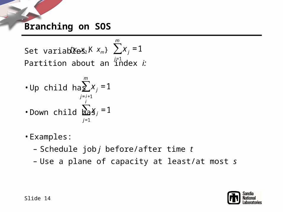
Branching on SOS

Set variables

Partition about an index i:

• Up child has

• Down child has

• Examples:

– Schedule job j before/after time t

– Use a plane of capacity at least/at most s

€

x1,x2,K xm{ }

€

x j

j=1

i

∑ =1

€

x j

j= i+1

m

∑ =1€

x j

j=1

m

∑ =1

Slide 15

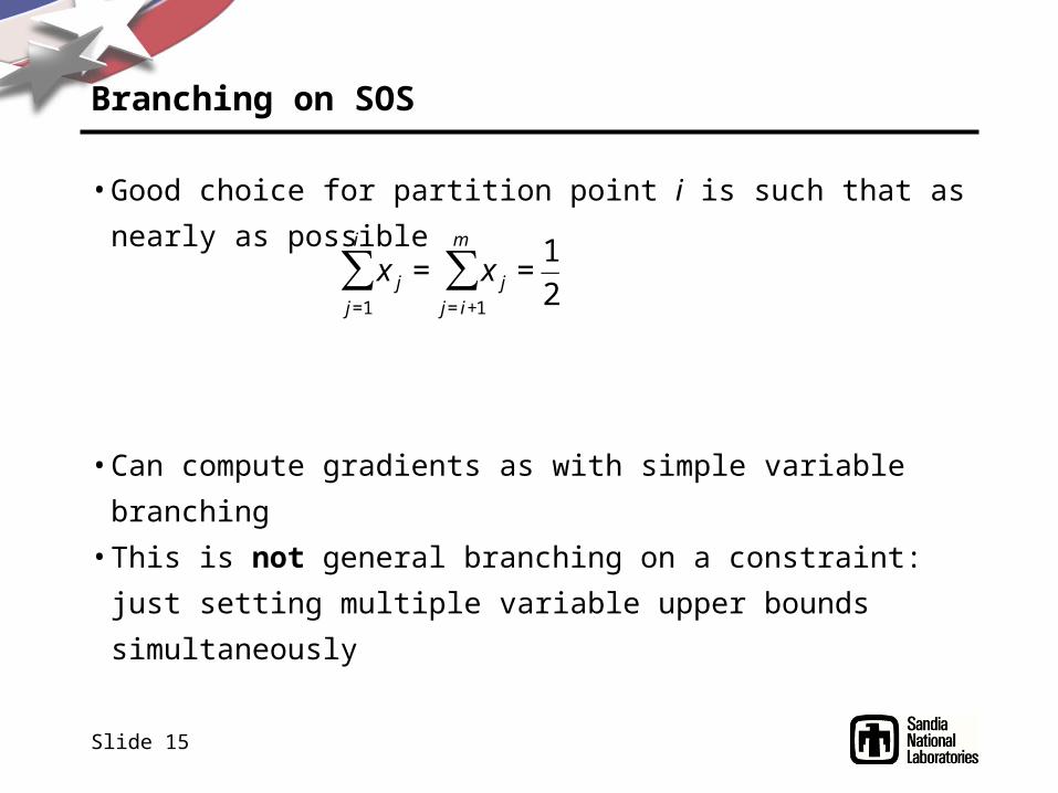
Branching on SOS

• Good choice for partition point i is such that as nearly as possible

• Can compute gradients as with simple variable branching

• This is not general branching on a constraint: just setting multiple

variable upper bounds simultaneously

€

x j

j=1

i

∑ = x j

j= i+1

m

∑ =1

2

Slide 16

Postponing Branching

Branching causes exponential growth of the search tree

Is there a way to make progress without branching?

Slide 17

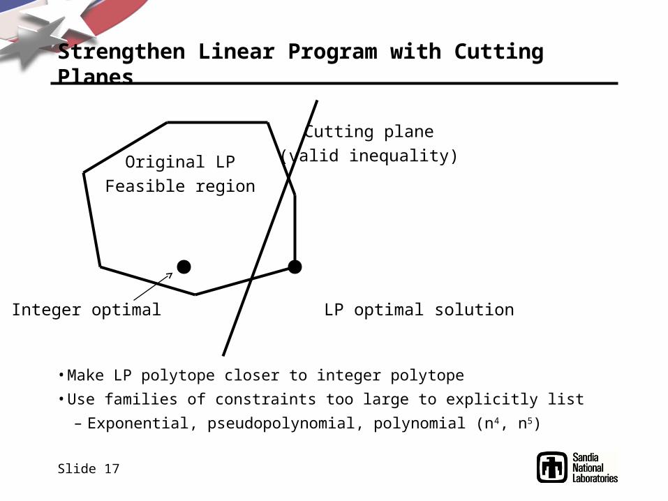
Strengthen Linear Program with Cutting Planes

Original LP

Feasible region

LP optimal solution

Cutting plane

(valid inequality)

Integer optimal

• Make LP polytope closer to integer polytope

• Use families of constraints too large to explicitly list

– Exponential, pseudopolynomial, polynomial (n4, n5)

Slide 18

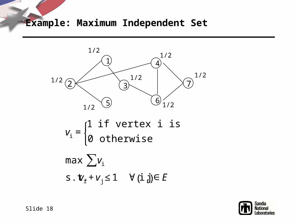
Example: Maximum Independent Set

2

1 4

7

5

3

6

vi =1 if vertex i is in the MIS

0 otherwise ⎧ ⎨ ⎩

max vi∑s.t. vi +vj ≤1 ∀ i, j( )∈E

1/2

1/2

1/2

1/2

1/2

1/2

1/2

Slide 19

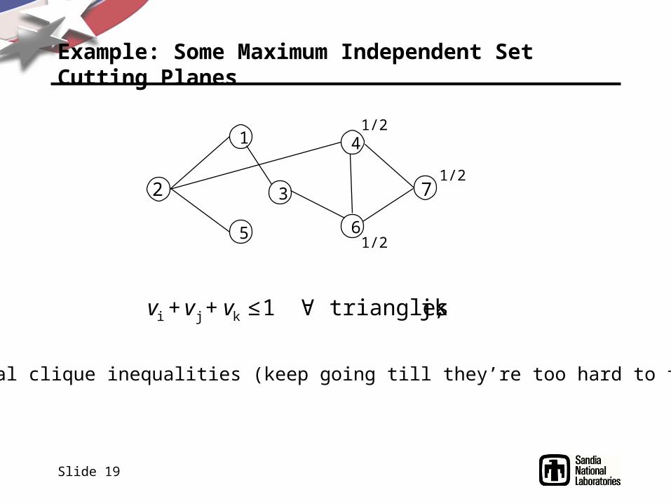
Example: Some Maximum Independent Set Cutting Planes

2

1 4

7

5

3

6

vi +vj +vk ≤1 ∀ triangles i,j,k

1/2

1/2

1/2

More general clique inequalities (keep going till they’re too hard to find)

Slide 20

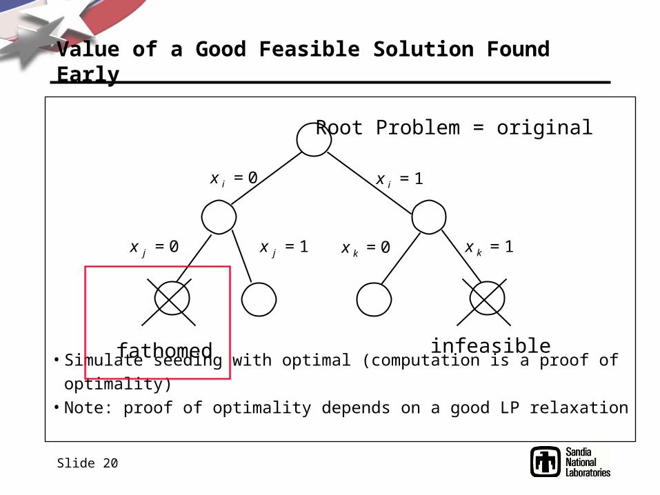
Value of a Good Feasible Solution Found Early

• Simulate seeding with optimal (computation is a proof of optimality)• Note: proof of optimality depends on a good LP relaxation

x k = 0 x k = 1

x i = 1

x j = 1 x j = 0

x i = 0

Root Problem = original

fathomed infeasible

Slide 21

Solving Subproblem LPs Quickly

• The LP relaxation of a child is usually closely related to its parent’s LP

• Exploit that similarity by saving the parent’s basis

Slide 22

Linear Programming Geometry

Optimal point of an LP is at a corner (assuming bounded)

feasible

€

cT x = opt

€

cT x = -∞

Slide 23

Linear Programming Algebra

What does a corner look like algebraically?

Ax=b

Partition A matrix into three parts

where B is nonsingular (invertible, square).

Reorder x: (xB, xL, xU)

We have BxB + LxL + UxU = b

B L U

Slide 24

Linear Programming Algebra

We have BxB + LxL + UxU = b

Set all members of xL to their lower bound.

Set all members of xU to their upper bound.

Let (this is a constant because bounds and u are)

Thus we have

Set

This setting of (xB, xL, xU) is called a basic solution

• A basic solution satisfies Ax=b by construction

If all xB satisfy their bounds ( ), this is a basic feasible

solution (BFS)

€

′ b = b − LxL −UxU

€

l

€

xB = B−1 ′ b

€

BxB = ′ b

€

l B ≤ xB ≤ uB

Slide 25

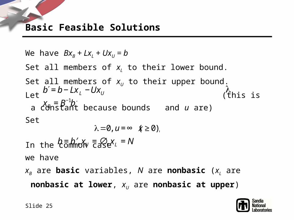
Basic Feasible Solutions

We have BxB + LxL + UxU = b

Set all members of xL to their lower bound.

Set all members of xU to their upper bound.

Let (this is a constant because bounds and u are)

Set

In the common case

we have

xB are basic variables, N are nonbasic (xL are nonbasic at lower, xU are

nonbasic at upper)

€

xB = B−1 ′ b

€

′ b = b − LxL −UxU

€

l =0, u = ∞ (x ≥ 0),

€

b = ′ b , xU =∅ , xL = N

€

l

Slide 26

Algebra and Geometry

A BFS corresponds to a corner of the feasible polytope:

m inequality constraints (plus bounds) and n variables. Polytope in n-

dimensional space. A corner has n tight constraints.

With slacks Ax + IxS = b

m equality constraints (plus bounds) in n+m variables. A BFS has n tight

bound constraints (from the nonbasic variables).

€

Ax ≤ b

Slide 27

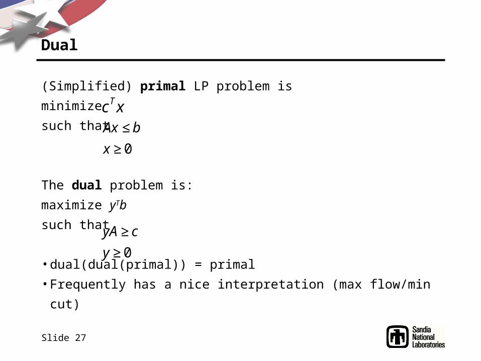
Dual

(Simplified) primal LP problem is

minimize

such that

The dual problem is:

maximize yTb

such that

• dual(dual(primal)) = primal

• Frequently has a nice interpretation (max flow/min cut)

cTx

€

€

Ax ≤ b

x ≥ 0

€

yA ≥ c

y ≥ 0

Slide 28

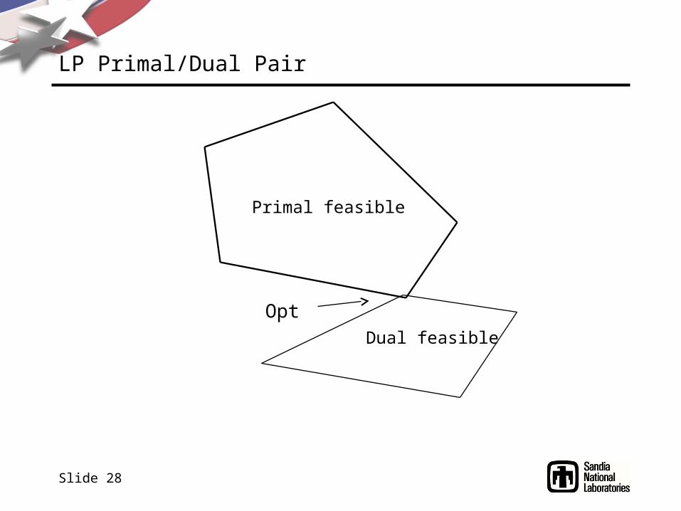
LP Primal/Dual Pair

Primal feasible

Dual feasible

Opt

Slide 29

Parent/Child relationship (intuition)

Parent optimal pair (x*,y*)

• Branching reduces the feasible region of the child LP with respect to its

parent and increases the dual feasible region

• y* is feasible in the child’s dual LP and it’s close to optimal

Resolving the children using dual simplex, starting from the parent’s

optimal basis can be at least an order of magnitude faster than starting

from nothing.

Note: Basis can be big. Same space issues as with knapsack example.