Reconfigurable Wheels:

Re-Inventing the Wheel for the Next Generation of Planetary Rovers

by

Brittany Baker

B.S. Aeronautics and Astronautics

Massachusetts Institute of Technology, 2008

Submitted to the Department of Aeronautics and Astronautics in Partial Fulfillment of the

Requirements for the Degree of

Master of Science in Aeronautics and Astronautics

at the

MASSACHUSETTS INSTITUTE OF TECHNOLOGY

February 2012

© Massachusetts Institute of Technology 2012. All rights reserved.

Author…………………………………………………………………………………………………………………………………….

Department of Aeronautics and Astronautics

February 2, 2012

Certified by………………………………………………………………………………………………………………………………

Olivier L. de Weck

Associate Professor of Aeronautics and Astronautics

Associate Professor of Engineering Systems

Thesis Supervisor

Accepted by…………………………………………………………………………………………………………………………….

Eytan H. Modiano

Professor of Aeronautics and Astronautics

Chair, Committee on Graduate Students

2

3

Reconfigurable Wheels:

Re-Inventing the Wheel for the Next Generation of Planetary Rovers

by

Brittany Baker

Submitted to the Department of Aeronautics and Astronautics on February 2, 2012 in Partial

Fulfillment of the Requirements for the Degree of Master of Science in Aeronautics and

Astronautics

Abstract

Experiences with Spirit and Opportunity, the twin Mars Exploration Rovers, showed that one of the

major issues that needs to be addressed in order to expand the exploration capabilities of planetary

rovers is that of wheel traction. The relationships governing how much traction a wheel can produce are

highly dependent on both the shape of the wheel and terrain properties. These relationships are

complex and not yet fully understood. The amount of power required to drive a wheel is also dependent

on its shape and the terrain properties. Wheel sizes that tend to maximize traction also tend to require

more power. In the past, it has always been a challenge to find the right balance between designing a

rover wheel with high traction capabilities and low power requirements. More recently, researchers

invented the idea of a reconfigurable wheel which would have the ability to change its shape to adapt to

the type of terrain it was on. In challenging terrain environments, the wheel could configure to a size

that would maximize traction. In less challenging terrain environments, the wheel could configure to a

size that would minimize power. Theoretical simulation showed that the use of reconfigurable wheels

could improve tractive performance and some initial prototyping and experimental testing corroborated

those findings. The purpose of this project was to extend that prototyping and experimenting. Four

reconfigurable wheels were designed, built, and integrated onto an actual rover platform. A control

methodology whereby the wheels could autonomously reconfigure was also designed, implemented,

and demonstrated. The rover was then tested in a simulated Martian environment to assess the

effectiveness of the reconfigurable wheels. During the tests, the power consumption and the distance

traveled by the rover were both measured and recorded. In all tests, the wheels were able to

successfully reconfigure and the rover continued to advance forward; but as was expected, the

reconfigurable wheel system consumed more power than a non-reconfigurable wheel system. In the

end, the results showed that if maximizing vehicle traction was weighed more heavily than minimizing

power consumption, the use of reconfigurable wheels yielded a net gain in performance.

Thesis Supervisor: Olivier L. de Weck

Title: Associate Professor of Aeronautics and Astronautics and Engineering Systems

4

5

Acknowledgements

This project would not have been possible without the support of many people and I would be remiss if I

did not publicly express my thanks to a number of individuals. First, I would like to thank my advisor,

Olivier de Weck. I had the privilege of working with Professor de Weck as part of my 62x project and was

grateful for the chance to continue working on this project with him as a graduate student. I am grateful

for all of his support and guidance.

Secondly, I would like to thank Jessica Duda of Aurora Flight Sciences. Jessica served as a mentor for me

throughout the course of this project. Her assistance and guidance were invaluable to me, especially

during the time that Professor de Weck was on sabbatical. Jessica provided a lot of encouragement and

support when things went wrong. She not only helped me solve technical issues specific to my project

but also taught me how to be a better engineer in general.

Thirdly, I owe enormous thanks to Todd Billings, Dave Robertson, and Dick Perdichizzi. The three of

them constitute the Aero/Astro technical lab staff. I never would have been able to finish my project

without their advice and help. I spent many hours in the machine shop, Gelb lab, and hangar, and even

when my parts broke or blew up, Todd and Dave kept me laughing the entire time and helped me push

through a lot of discouraging and frustrating moments.

I owe a huge thanks to my friends Donna Hunter, Cynthia Furse, Stephanie Ketchum, David Lazzara, John

Gardner, Lisa Clarke, Marytheresa Ifediba, and Bill and Jo Maitland. Each of these people has provided

me with tremendous support, encouragement and love. Their small acts of kindness often came when I

most needed it. In moments of self-doubt or discouragement they patiently listened to me, cheered me

on, and kept believing in me even when I lost belief in myself. I am eternally in their debt.

Last, but certainly not least, I would like to thank my parents and siblings. My family is eternal and one

of the greatest blessings I have ever been given in life. I was born of goodly parents who raised me in the

ways of truth and righteousness. Their love for me is unconditional, their sacrifices innumerable, and I

could never do enough to sufficiently repay them for all that they have done and continue to do for me.

6

7

Table of Contents Nomenclature ............................................................................................................................................. 15

1.0 Introduction .......................................................................................................................................... 17

1.1 Motivation ......................................................................................................................................... 17

1.2 Objective and Goals .......................................................................................................................... 18

2.0 Background Research and Previous Work ............................................................................................ 19

2.1 Past Rovers and Their Wheels........................................................................................................... 19

2.2 Terramechanics ................................................................................................................................. 24

2.3 Concept Development ...................................................................................................................... 28

2.4 62x project ....................................................................................................................................... 29

3.0 Conceptual Design and Development ................................................................................................... 32

3.1 General Challenges and Influence Diagram ...................................................................................... 32

3.2 Three Different Wheel Designs ......................................................................................................... 33

3.3 Wheel Sizing and Simulation ............................................................................................................. 37

3.4 Strength Modeling (Deflection and Force) ....................................................................................... 39

Simple Beam Theory: .......................................................................................................................... 39

Simple Beam Theory Results ............................................................................................................... 40

3.5 Reconfigurability Metrics .................................................................................................................. 42

3.6 Design Selection ................................................................................................................................ 44

4.0 Fabrication and Assembly ..................................................................................................................... 45

4.1 Rover Platform Selection .................................................................................................................. 45

4.2 Material and Part Selection .............................................................................................................. 45

4.3 Wheels and Platform Integration ..................................................................................................... 47

4.4 Assembly ........................................................................................................................................... 50

4.5 Initial Drive Testing ........................................................................................................................... 53

5.0 Integration, Autonomy, and Control ..................................................................................................... 56

5.1 Electrical System Overview ............................................................................................................... 56

5.2 System Integration and Preliminary Testing ..................................................................................... 56

5.3 Control Methodology ........................................................................................................................ 61

5.4 A Systems Engineering Perspective .................................................................................................. 63

6.0 Testing and Results ............................................................................................................................... 66

6.1 Test Set-Up ........................................................................................................................................ 66

8

6.2 Testing Procedure ............................................................................................................................. 67

6.3 Test Results ....................................................................................................................................... 68

6.4 Error Analysis .................................................................................................................................... 78

6.5 Summary of Results .......................................................................................................................... 80

7.0 Summary and Conclusions .................................................................................................................... 81

7.1 Conclusion ......................................................................................................................................... 81

7.2 Future Work ...................................................................................................................................... 81

7.3 Closing Statement ............................................................................................................................. 83

8.0 References ............................................................................................................................................ 84

9.0 Appendix ............................................................................................................................................... 86

9

List of Figures

Figure 1 - Opportunity's wheel stuck in the sand (Image Courtesy of NASA) ............................................ 17

Figure 2 - Side view of a LRV wheel (Image Courtesy of NASA) .................................................................. 20

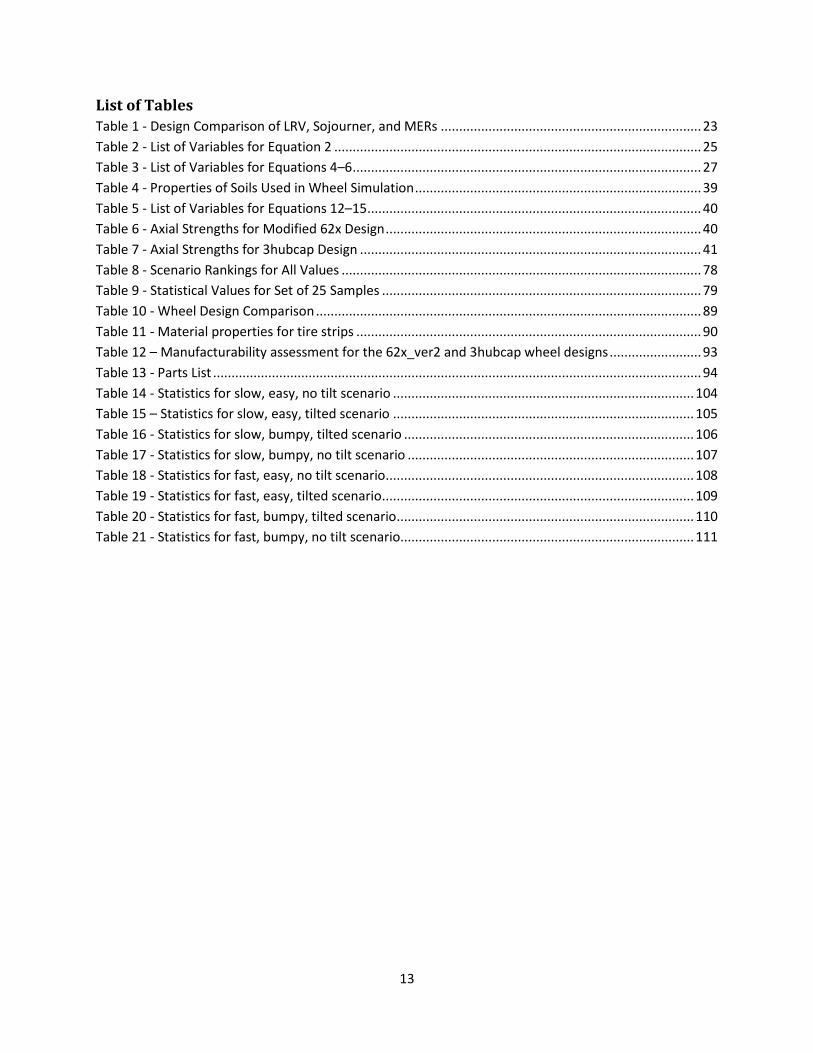
Figure 4 - Astronaut Eugene Cernan driving LRV on Apollo 17 (Image courtesy of NASA) ........................ 21

Figure 3 - A worker hand weaves wire for LRV wheel (Image Courtesy of NASA) ..................................... 21

Figure 5 - JPL engineer with Sojourner rover in front and one of the MERs in back (Image courtesy of

NASA) .......................................................................................................................................................... 22

Figure 6 - Evolution of Rover Wheels: MER wheel on the left, Sojourner wheel in the center and MSL

wheel on the right (Image courtesy of NASA) ............................................................................................ 24

Figure 7 - Diagram of wheel/soil interactions (Image courtesy of [9]) ....................................................... 26

Figure 8 - 62x Testing Apparatus ................................................................................................................ 30

Figure 9 - 62x Test Matrix ........................................................................................................................... 30

Figure 10 - Influence Diagram ..................................................................................................................... 33

Figure 11 - SolidWorks model of first wheel design ................................................................................... 34

Figure 12 - SolidWorks model of second wheel design .............................................................................. 35

Figure 13 - SolidWorks model for third wheel design ................................................................................ 36

Figure 14 - Objective function graph for dry sand ...................................................................................... 37

Figure 15 - Objective function graph for sandy loam I ............................................................................... 38

Figure 16 - Graph of J=0 contours ............................................................................................................... 38

Figure 17 - Pin supported arch for thin curved beam theory (Image courtesy of [15]) ............................. 42

Figure 18 - VEX Robot ................................................................................................................................. 45

Figure 19 - Composite tire strips made from spring steel and copper mesh ............................................. 46

Figure 20 - Aluminum hubcap and ring flange ............................................................................................ 47

Figure 21 - Linear actuator used in reconfigurable wheel .......................................................................... 47

Figure 22 - Wheel Attachment Design ........................................................................................................ 48

Figure 23 - Wheel axle attachment ............................................................................................................. 49

Figure 24 - Copper electric slip rings mounted to outside of inner hubcap ............................................... 49

Figure 25 - Wire brushes for slip rings ........................................................................................................ 50

Figure 26 - Wheel axle, hollow tube, and inner hubcap all pinned together ............................................. 52

Figure 27 - Linear actuator mounted to inner hubcap ............................................................................... 52

Figure 28 - Securing the tire strips .............................................................................................................. 53

Figure 29 - The first assembled wheel ........................................................................................................ 53

Figure 30 - Rover with four reconfigurable wheels and support bars ........................................................ 54

Figure 31 - Wheel with hand-sewn spandex cover ..................................................................................... 55

Figure 32 - Custom made collar to connect leadscrew, bearing/mounts, and hubcaps ............................ 58

Figure 33 - Bearing and bearing mount for support arch ........................................................................... 58

Figure 34 - Frictionless rails mounted to rover frame ................................................................................ 59

Figure 35 - Rover with new support arches ................................................................................................ 59

Figure 36 - Close-up of rail, cart, and arch .................................................................................................. 60

Figure 37 - Close-up of new hubcap attachment ........................................................................................ 60

Figure 38 - Charred remains of a motor driver after it exploded ............................................................... 61

10

Figure 39 - Flowchart for reconfiguration control algorithm...................................................................... 63

Figure 40 - Design structure matrix for rover system ................................................................................. 64

Figure 41 - Testing in the homemade Mars yard filled with pea gravel and popcorn ................................ 67

Figure 42 - Text matrix of testing procedures............................................................................................. 68

Figure 43 - Total average distance with reconfiguration for test scenarios ............................................... 70

Figure 44 - Average additional distance traveled due to reconfiguration for test scenarios ..................... 70

Figure 45 – Average percentage increase in distance due to reconfiguration for test scenarios .............. 71

Figure 46 - Average power consumed with reconfiguration for test scenarios ......................................... 72

Figure 47 - Average increase in power due to reconfiguration for test scenarios ..................................... 72

Figure 48 - Average percentage increase in power due to reconfiguration for test scenarios .................. 73

Figure 49 - J* values for different alpha values in test scenarios ............................................................... 75

Figure 50 - Efficiency calculations for all testing scenarios ......................................................................... 76

Figure 51 - Relative efficiency values for all test scenarios ........................................................................ 77

Figure 52 - Potential test diagram for future testing .................................................................................. 82

Figure 53 - Image Collage: MER on the left, reconfigurable wheel rover on the right, Apollo 1 Hills in the

background (MER and Apollo 1 Hills pictures courtesy of NASA) ............................................................... 83

Figure 54 - Earlier version of the influence diagram ................................................................................... 86

Figure 55 - Influence diagram with variables .............................................................................................. 87

Figure 56 - Incidence matrix showing dependencies between relevant variables ..................................... 88

Figure 57 - Simple beam theory deflection results for 3hubcap wheel design. The different colors

represent different tire strip lengths. The x-axis is the distance along the length of the tire strip and the

y-axis is the amount of deflection............................................................................................................... 91

Figure 58 - Simple beam theory deflection results for 62x_ver2 wheel design. The different colors

represent different tire strip lengths. The x-axis is the distance along the length of the tire strip and the

y-axis is the amount of deflection............................................................................................................... 91

Figure 59 - Thin curved beam theory deflection results for the 3hubcap wheel design. The different

colors represent different tire strip lengths. The x-axis is the distance along the length of the tire strip

and the y-axis is the amount of deflection. ................................................................................................ 92

Figure 60 - Thin curved beam theory results for the 62x_ver2 wheel design. The different colors

represent different tire strip lengths. The x-axis is the distance along the length of the tire strip and the

y-axis is the amount of deflection............................................................................................................... 92

Figure 61 - Dimensional drawings of inner hubcap and aluminum plug .................................................... 96

Figure 62 - Dimensional drawing for bearings for hollow steel tube ......................................................... 97

Figure 63 - Dimensional drawing for support arms .................................................................................... 97

Figure 64 - Dimensional drawing of collars and vertical mounts for outside hubcaps............................... 98

Figure 65 - Specification sheet for linear actuator ..................................................................................... 99

Figure 66 - Specification sheet for stepper motor driver ......................................................................... 100

Figure 67 - Stepper motor diagrams ......................................................................................................... 101

Figure 68 - All of the connections for the electrical system ..................................................................... 102

Figure 69 - Power and distance data for slow, easy, no tilt scenario ....................................................... 104

Figure 70 - Power and distance data for slow, easy, tilted scenario ........................................................ 105

Figure 71 - Power and distance data for slow, bumpy, tilted scenario .................................................... 106

11

Figure 72 - Power and distance data for slow, bumpy, no tilt scenario ................................................... 107

Figure 73 - Power and distance data for fast, easy, no tilt scenario ......................................................... 108

Figure 74 - Power and distance data for fast, easy, tilted scenario .......................................................... 109

Figure 75 - Power and distance data for fast, bumpy, tilted scenario ...................................................... 110

Figure 76 - Power and distance data for fast, bumpy, no tilt scenario ..................................................... 111

Figure 77 - Power difference vs. distance difference for all tests ............................................................ 112

12

13

List of Tables

Table 1 - Design Comparison of LRV, Sojourner, and MERs ....................................................................... 23

Table 2 - List of Variables for Equation 2 .................................................................................................... 25

Table 3 - List of Variables for Equations 4–6 ............................................................................................... 27

Table 4 - Properties of Soils Used in Wheel Simulation .............................................................................. 39

Table 5 - List of Variables for Equations 12–15 ........................................................................................... 40

Table 6 - Axial Strengths for Modified 62x Design ...................................................................................... 40

Table 7 - Axial Strengths for 3hubcap Design ............................................................................................. 41

Table 8 - Scenario Rankings for All Values .................................................................................................. 78

Table 9 - Statistical Values for Set of 25 Samples ....................................................................................... 79

Table 10 - Wheel Design Comparison ......................................................................................................... 89

Table 11 - Material properties for tire strips .............................................................................................. 90

Table 12 – Manufacturability assessment for the 62x_ver2 and 3hubcap wheel designs ......................... 93

Table 13 - Parts List ..................................................................................................................................... 94

Table 14 - Statistics for slow, easy, no tilt scenario .................................................................................. 104

Table 15 – Statistics for slow, easy, tilted scenario .................................................................................. 105

Table 16 - Statistics for slow, bumpy, tilted scenario ............................................................................... 106

Table 17 - Statistics for slow, bumpy, no tilt scenario .............................................................................. 107

Table 18 - Statistics for fast, easy, no tilt scenario .................................................................................... 108

Table 19 - Statistics for fast, easy, tilted scenario ..................................................................................... 109

Table 20 - Statistics for fast, bumpy, tilted scenario ................................................................................. 110

Table 21 - Statistics for fast, bumpy, no tilt scenario................................................................................ 111

14

15

Nomenclature

Abbreviations

CAD computer aided design

GMDRL General Motors Defense Research Laboratory

JPL Jet Propulsion Laboratory

LRV Lunar Roving Vehicle

MER Mars Exploration Rover

MIT Massachusetts Institute of Technology

MSFC Marshall Space Flight Center

MSL Mars Science Laboratory

NASA National Aeronautics and Space Administration

Roman Symbols

A contact area of wheel (for terramechanics)

A closed area of wire mesh (for simple beam theory)

Ass relative area of spring steel

b wheel width

b1 length of beam

b2 spring steel width

b3 wire mesh width

c cohesion

D wheel diameter

D* distance

DP drawbar pull

E modulus

Ess spring steel modulus

Ecw copper wire modulus

Ef relative functional efficiency

Ep relative performance efficiency

F tractive force

h1 spring steel thickness

h2 wire mesh thickness

I inertia

Icw copper wire inertia

Iss spring steel inertia

J objective function

J* alternative objective function

K shear deformation modulus

Kpc, Kpϒ Terzaghi soil factors

kc cohesive modulus of deformation

16

kφ frictional modulus of deformation

L length of contact area (for terramechanics)

L length of beam (for simple beam theory)

n soil constant

P power

P load on beam (for thin curved beam theory)

Pr buckling force

q uniform load on beam

R effective radius

Rb bulldozing resistance

Rc compaction resistance

s wheel slip

T torque

W wheel load

w deflection

z sinkage

Greek Symbols

α weighting function (for wheel performance)

α angle between horizontal surface and pin location (for thin curved beam theory)

ϒ soil density

θ1 angle from vertical to point of soil contact

θ2 angle from vertical to point of loss of soil contact

σ normal stress

ω angular velocity

τ soil shear strength

φ internal friction angle

17

1.0 Introduction

1.1 Motivation Forty three years ago, man successfully walked on a world other than the one that we call home. Since

that monumental moment, many have dreamed of the day when the world would watch man walk on

the surface of Mars. The challenges associated with getting to Mars are much greater than those

required for getting to the moon, but that does not mean the planet cannot still be explored in the

meantime. Probes and planetary rovers offer promising alternatives for exploring not only the moon and

Mars, but other celestial bodies as well.

These probes and rovers come with their own set of unique challenges. Issues of control, vision,

navigation, and communication must be handled differently for robotic exploration compared with

human exploration. In terms of navigation, it is much easier for a human explorer to assess terrain

conditions, decide how to navigate to their desired destination, or adapt to changing conditions than it

is for a rover to carry out those same tasks. However, successful navigation is imperative to effective

exploration, so the success of a robotic-based mission is largely dependent on the navigational

capabilities of the rover. For example, in 2005 one of the Mars Exploration Rovers (MERs), Opportunity,

got stuck in a sand pit (see Figure 1). It took engineers a month of painstaking effort to remove the

rover, which was almost lost in the process [1].

More recently, in May of 2009, Opportunity’s twin, Spirit, also got trapped in the sand and has remained

trapped there ever since. [2] Engineers eventually lost communication with the rover and it was officially

retired in May 2011. [3] Neither of the MERs can be considered a failure because they significantly

outperformed what they were initially designed to do. However, if robotic exploration of Mars is to

continue, rovers need to have better capability to

traverse challenging terrain, particularly soft soils such as

sand. There are multiple ways to enhance the mobility of

these rovers. One of the most promising avenues is to

design more effective wheels. This endeavor, though, is

complicated by the trade-offs that accompany any

engineering design problem. It would be easy to install

all-powerful, all-terrain wheels, but not without

significant setbacks in terms of weight, cost, and

complexity. As researchers reach toward the future and

look for ways to explore more interesting and challenging

places on the moon and Mars, it is clear that new and

more innovative engineering solutions need to be

developed to enhance the mobility of robotic explorers.

Figure 1 - Opportunity's wheel stuck in the sand (Image Courtesy of NASA)

18

1.2 Objective and Goals In response to the need to enhance robotic mobility, the purpose of this thesis is to investigate the use

of reconfigurable wheels on planetary rovers. Performing a complete evaluation of this concept is not

within the scope of this Master’s project. Rather, this thesis will seek to fulfill the following important

objectives:

1. Explore new design concepts for reconfigurable wheels

2. Select the best design and then build four working prototypes of that design

3. Integrate the four wheels onto a simulated rover platform to demonstrate proof of concept

4. Demonstrate ability of rover to autonomously reconfigure its wheels

5. Demonstrate and assess the effectiveness of using reconfigurable wheels while traversing a

simulated Martian environment

The first objective will be completed mainly through software-based analysis and assessment. The

remaining objectives will be hardware intensive and focus on the fabrication, assembly, integration, and

testing of the wheels.

This thesis will report on each successive phase of the project. The first section has outlined the project

goals. The second section will focus on past design considerations that have served as the foundation for

this work. The third section will describe the design process for this project. The building and assembly

procedures for the mechanical system will be set forth in the fourth section. The fifth section will focus

on the design and development of the electrical system. In the sixth section, the testing procedure will

be outlined followed by a discussion of the testing results. The seventh and final section will include a

project summary, conclusion, and discussion of future work.

19

2.0 Background Research and Previous Work

2.1 Past Rovers and Their Wheels Lunar Rovers

Work on the first planetary rovers began in the early 1960s as the U.S. turned its sights toward landing

men on the moon. Development of the lunar rover was mainly conducted under the direction of NASA’s

Marshall Space Flight Center (MSFC). Although development of the lunar rover was managed by MSFC,

many other major contractors, including Boeing Aircraft Corp., Bendix Corp., Grumman Aircraft

Engineering Corp., and Northrop Space Laboratories Inc., developed concepts for a lunar rover. At the

time, Dr. Mieczyslaw G. Bekker was regarded as the leading authority on land locomotion. He was in

charge of the Mobility Research Laboratory at General Motors Defense Research Laboratory (GMDRL) in

Santa Barbara, California, and was a key player in the development of some of the first concepts for a

lunar rover. Working with him were Samuel Romano, chief of Lunar and Planetary Programs at GMDRL,

and Ferenc Pavlics, a chief engineer in Romano’s group [4].

The first vehicle design concepts were being developed simultaneously with the logistics of actually

getting to the moon, so rover researchers originally operated under the assumption that a moon voyage

would consist of two separate launches—one to carry the crew and another to carry equipment. This

meant that weight restrictions were much more lenient and initial designs for lunar rovers were very

large—many on the order of about 3,000 kg. A critical development in the mid-1960s significantly

altered the rover designs: NASA decided that earth orbit rendezvous would be preferred over dual-

mode missions. This meant that the astronauts and their equipment would be transported together. As

a result, strict weight limits were imposed and the lunar rover could weigh no more than 227 kg (500

lbs) [4].

In the summer of 1965, a two-week conference was held in Falmouth, Massachusetts to outline a ten-

year plan for lunar exploration. As part of that plan, engineers and program managers agreed that any

surface roving vehicle would need to transport one to two crew members plus a scientific payload a

distance of at least 8 km. Design concepts and mobility studies continued to be carried out, but it was

not until four years later—only a few days before the historic Apollo 11 landing, in fact—that NASA

issued a formal request for proposals for a Lunar Roving Vehicle (LRV). There were 22 specific

requirements for the LRV [4]. Those relevant to the wheels included:

the maximum weight of the vehicle was to be no more than 400 lbs

the vehicle would have four wheels and each wheel would be individually driven using battery

powered electric motors

the carrying capacity was to be 840 lbs

the total range of the LRV had to be 120 km

the LRV had to have an operational lifetime of 78 hours on the lunar surface

the speed range of the fully loaded vehicle was to be 0–16 km/hr

the vehicle had to be capable of traversing slopes of up to 25 degrees

20

the vehicle had to be capable of

negotiating obstacles up to 30 cm high and

crevasses 70 cm wide

Four different contractors submitted

proposals for the LRV; ultimately the Boeing

Co. won the contract. They had less than

two years to design, build, and test the LRV,

which needed to be delivered to Kennedy

Space Center in April 1971.

The entire LRV was a work of engineering

genius (see Figure 2). The vehicle worked

virtually flawlessly on all of its missions

despite the fact that there was limited

knowledge available regarding the surface

and soil conditions on the moon. The

vehicle’s mobility success was largely

attributed to the eloquent wheel design.

The design came largely from the initial research and development conducted during the early 1960s as

part of NASA’s various lunar mobility programs. A major portion of this work was done at GM’s Defense

Research Laboratories (GMDRL) in Santa Barbara [4].

Two different designs were initially considered for the final product. The first design was a metal-elastic

wheel with a flat metal tread and a complex of interior circular cross-section metal springs. The second

design consisted of a wire frame with interior hoops and a solid aluminum rim. The second design was

eventually selected. Ferenc Pavlics, one of the chief engineers at GMDRL, described the challenges of

the wheel design as such: “We had to invent an all-metallic but still flexible wheel. Since this was a

manned vehicle going at a reasonable speed over rugged terrain, it had to provide the astronauts with a

good ride quality. So, the wheel had to be flexible and have good flotation over the soft lunar

terrain....We tried many different types and different materials, and finally nailed down this

configuration which was a flexible wire frame-type of wheel. The behavior of the wheel was like a low-

pressure pneumatic tire. It was flexible and it had a good footprint over the soft terrain so it didn’t sink

into the soil. At the same time, it provided a certain amount of damping because the interwoven tires,

as they deformed, had a friction at the joints, so it didn’t bounce like a spring would.” [4]

The wheel diameter was 81.3 cm and the width was 22.8 cm. The finished wheel weighed a mere 5.4 kg

and the nominal static load on each wheel, including the weight of the vehicle, the astronauts, and the

equipment, was 147 kg. The tire’s wire frame was made out of 0.84 mm diameter steel spring wire. 800

strands, each 81.3 cm long, were hand-woven using a special loom so that there was no seam anywhere

along the curved surface (see Figure 3). Riveted to the wire mesh were titanium tread strips in a specific

chevron pattern that provided 50 percent coverage of the contact patch. The inner circumferential ring

Figure 2 - Side view of a LRV wheel (Image Courtesy of NASA)

21

and titanium hoop springs created a secondary frame that helped

prevent wheel collapse under the impact of lunar rocks. Extensive

testing was done on the LRV wheels, including tests involving lunar soil

simulants and tests on a KC-135 flying a parabolic profile to simulate

the moon’s one-sixth gravity environment [4].

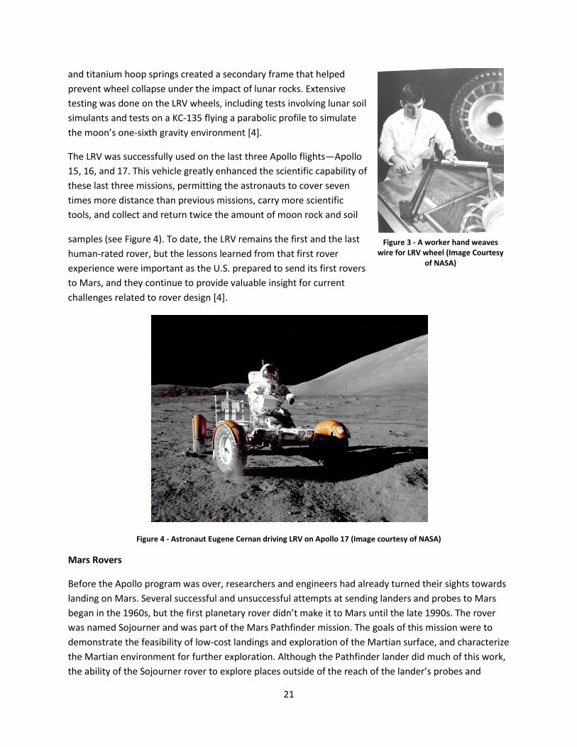
The LRV was successfully used on the last three Apollo flights—Apollo

15, 16, and 17. This vehicle greatly enhanced the scientific capability of

these last three missions, permitting the astronauts to cover seven

times more distance than previous missions, carry more scientific

tools, and collect and return twice the amount of moon rock and soil

samples (see Figure 4). To date, the LRV remains the first and the last

human-rated rover, but the lessons learned from that first rover

experience were important as the U.S. prepared to send its first rovers

to Mars, and they continue to provide valuable insight for current

challenges related to rover design [4].

Figure 4 - Astronaut Eugene Cernan driving LRV on Apollo 17 (Image courtesy of NASA)

Mars Rovers

Before the Apollo program was over, researchers and engineers had already turned their sights towards

landing on Mars. Several successful and unsuccessful attempts at sending landers and probes to Mars

began in the 1960s, but the first planetary rover didn’t make it to Mars until the late 1990s. The rover

was named Sojourner and was part of the Mars Pathfinder mission. The goals of this mission were to

demonstrate the feasibility of low-cost landings and exploration of the Martian surface, and characterize

the Martian environment for further exploration. Although the Pathfinder lander did much of this work,

the ability of the Sojourner rover to explore places outside of the reach of the lander’s probes and

Figure 3 - A worker hand weaves wire for LRV wheel (Image Courtesy

of NASA)

22

cameras was invaluable. This rover was relatively small, with a total mass of 10.5 kg and wheels that

were only 13 cm in diameter and 7 cm wide. The speed of the rover was also slow, traveling only 1 cm

per second. The most notable feature of this rover was the rocker-bogie suspension system. This was a

six-wheeled suspension system developed in the garage of a JPL engineer, Don Bickler. This ingenious

design permitted a rover to surmount virtually all potential obstacles while remaining stable.

The Sojourner rover roamed around the Martian surface for about two and a half months before

engineers lost contact with it. During that time, it traveled 104 meters and collected a plethora of

pictures and data that it relayed back to scientists on earth. The successful demonstration of the

Sojourner rover paved the way for the next, much larger Mars Exploration Rover (MER) program [4, 5].

Spirit and Opportunity were the twin rovers that debuted after Sojourner. These rovers were much

larger, each weighing 174 kg. Similar to Sojourner, these rovers had six individually-driven wheels and a

rocker-bogie suspension system (see Figure 5). Chris Vorhees, one of the primary engineers in charge of

the MERs mobility system, described the process and challenge of designing new wheels for these

rovers: “We started with the Sojourner wheels as a base to work from. Because of many different

engineering demands on the wheels, the wheels for our new rovers didn’t mature until late in the game.

A big challenge was to be able to get enough traction to get through soil and over rocks but also to be

benign enough to get off the lander without getting tangled in the deflated airbags.” [4]

After lots of modeling, simulation, analysis, prototyping, and testing, the mobility team settled on a final

design for the wheels. Each wheel was machined from a single solid piece of aluminum and curved along

the entire circumferential surface to maintain uniform contact with the Martian surface. The wheels

were 26 cm in diameter and featured spiral flexures in the hubs that served as built-in shock absorbers.

The flexures were filled with a special foam material called solimide that remained flexible even in the

extreme Martian temperatures. The foam also protected the drive and steering actuators inside the

wheel [4, 5].

Figure 5 - JPL engineer with Sojourner rover in front and one of the MERs in back (Image courtesy of NASA)

23

Spirit was launched first in July of 2003. Opportunity followed three months later, and both rovers

successfully landed on the Martian surface in 2004. The mission lifetime of the rovers was designed to

be only 90 days, but both rovers far outlasted that time frame [5]. Engineers recently lost contact with

Spirit and it was officially retired in May 2011, but as of this writing, Opportunity continues to operate

on the red planet’s surface, more than eight years after its landing [6]. Together these two rovers have

traveled more than 20 km on the Martian surface and explored a variety of terrain, rocks, hills and

craters. They have sent back more than a quarter million images and thousands of scientific spectra.

Arguably, their most noteworthy contribution is that their analysis and findings have led to the

conclusion that at one time water was present on the planet’s surface. Although these rovers have been

highly successful and able to explore an exceptional amount of terrain, both have faced numerous

mobility problems. There are still many locations on the planet’s surface that scientists desire to explore,

but doing so requires that future rovers be equipped with better mobility systems. Table 1 provides a

side by side design comparison for the LRV, Sojourner, and the MERs (also see Figure 6).

The most recent Mars rover is the Mars Science Laboratory (MSL). It launched in November 2011 and is

scheduled to land on Mars in August 2012. It is much bigger than the MERs, with an estimated mass of

approximately 775 kg. This rover features an even more efficient rocker-bogie suspension system with

wheel diameters of 40 cm and the capability to roll over 75 cm-high obstacles. These wheels are very

similar to the wheels on the MERs and their effectiveness at navigating through the rough Martian soil is

yet to be determined [5].

Table 1 - Design Comparison of LRV, Sojourner, and MERs

Rover Physical Sizes Notable Features

Sojourner

b = 7 cm D = 13 cm Rover mass: 10.5 kg

- Traction provided by metal wheels with metal spikes - Rocker-bogie suspension system

MERs (Mars

Exploration Rovers)

D = 26 cm Rover mass: 174 kg

- Aluminum wheels - Shock-absorption provided by spiral flexures in wheel hubs - Uniform contact with planet surface maintained due to uniform curvature of entire circumferential surface - Rocker-bogie suspension system

LRV (Lunar Roving

Vehicle)

b = 22.8 cm D = 81.3 cm Wheel mass: 5.5 kg Rover mass: 210 kg Static load per wheel: 147 kg

- Wheel rim made out of 2024-T4 aluminum alloy - Seamless wire mesh for tire were hand-woven in special loom using 800 strands of wire, each 81.3 cm long and 0.84 mm in diameter - Titanium tread strips were riveted to wire mesh in a specific chevron pattern to provide 50% coverage of contact patch - Wire mesh and titanium tread were riveted to wheel disc - Dynamic impact forces absorbed by a secondary wheel made out of circumferential ring and titanium hoop springs

24

Figure 6 - Evolution of Rover Wheels: MER wheel on the left, Sojourner wheel in the center and MSL wheel on the right (Image courtesy of NASA)

2.2 Terramechanics In order to design an effective wheel, it is imperative to understand the interactions that occur between

a wheel and the ground it is in contact with. This field of study is called terramechanics. This field can be

further divided into other sub-categories. For instance, the equations that describe wheel behavior for

pneumatic wheels are different than those for non-pneumatic (i.e., rigid) wheels. Additionally, the

parameters most significant for road-based wheels differ from those most significant for off-road

vehicles [7-10]. The equations and principles discussed here will focus on rigid wheels for off-road

vehicles.

In general, there are three principal elements that control or contribute to vehicle mobility:

vehicle type and loading conditions

surface cover and surface layer properties

geometric terrain features

In order to achieve optimum mobility, the vehicle must be able to move from one point to another with

the least amount of wasted motion and energy. The vehicle must be able to “float” on top of the terrain,

which requires that the terrain provide sufficient support and strength. Otherwise, the wheels sink into

the soil. The wheel must also provide sufficient resistance (i.e., friction) so that thrust can develop

between the wheels and terrain with minimal loss due to slippage. The greater the ability of these

wheel-terrain interactions to transfer the thrust into the substrate, the more traction the vehicle is able

to generate. Vehicle slip happens when the vehicle cannot propel itself forward because it is unable to

“grip” the substrate by transferring the surface slip motion to substrate thrust. There are three main

ways that the vehicle can become immobilized [7-10]:

there is too much sinkage due to lack of terrain strength

25

excessive slippage occurs even though adequate flotation exists

slip-sinkage behavior occurs where continued slippage causes the wheels to “dig” into the soil

and exacerbate sinkage

All of these interactions are quite complex and developing equations to accurately model them remains

an active area of research. One of the reasons why modeling these behaviors is so difficult is because

there are many variables that play a role in these interactions. Everything from the geometry and

structural properties of the wheel to the environmental conditions and structural properties of the soil

influence how much traction the wheel is able to create. To date, the most commonly accepted and

used model for off-road vehicles is that developed by Bekker, one of the engineers who was an active

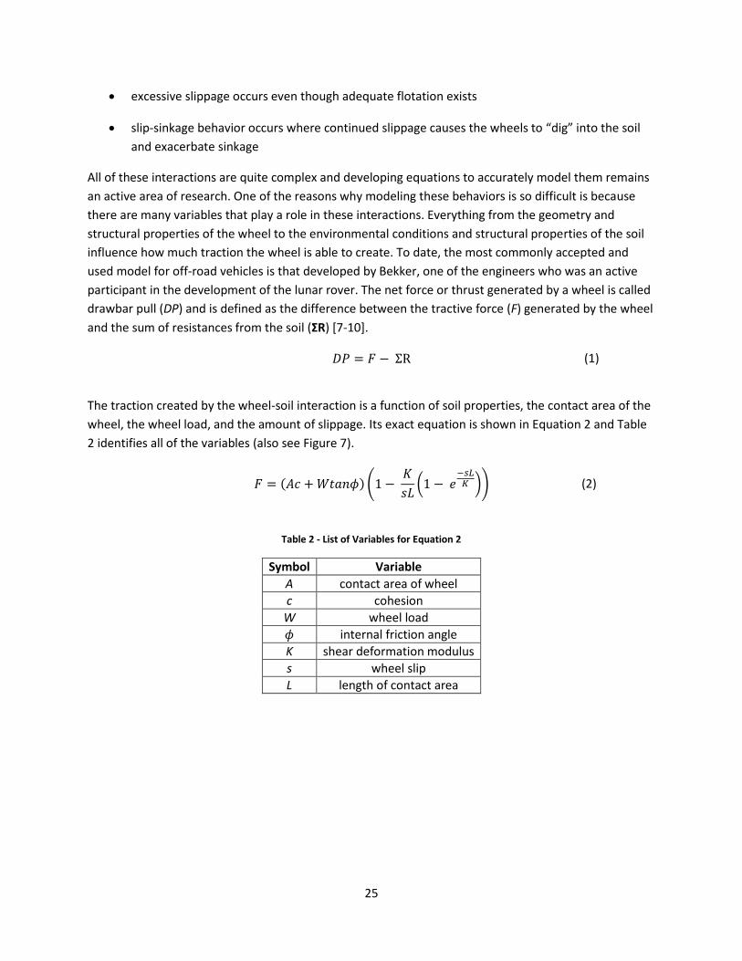
participant in the development of the lunar rover. The net force or thrust generated by a wheel is called

drawbar pull (DP) and is defined as the difference between the tractive force (F) generated by the wheel

and the sum of resistances from the soil (ΣR) [7-10].

(1)

The traction created by the wheel-soil interaction is a function of soil properties, the contact area of the

wheel, the wheel load, and the amount of slippage. Its exact equation is shown in Equation 2 and Table

2 identifies all of the variables (also see Figure 7).

(2)

Table 2 - List of Variables for Equation 2

Symbol Variable

A contact area of wheel

c cohesion

W wheel load

internal friction angle

K shear deformation modulus

s wheel slip

L length of contact area

26

It is important to note that there is a limit to how much

tractive force or thrust can be exerted from the soil.

Every soil has a failure point—the equivalent to hitting a

region of plastic deformation. As a vehicle attempts to

drive forward, it exerts a certain amount of stress on the

soil. However, if the stress level exceeds a certain point,

the soil will experience a structural failure and thrust

will not be generated from the wheel-soil interaction.

One of the more commonly used metrics to describe

this failure point is the Mohr-Coulomb Criterion, which

estimates the shear strength of soil (τ) as a function of

soil cohesion (c), internal friction angle ( ), and the

normal stress exerted on the surface ( ). Cohesion describes the bond that cements particles together

irrespective of internal normal pressures between individual particles. Some soils, such as clay, have

very high cohesion; in fact, their shear strength mostly comes from cohesion. Other soils, particularly dry

sand, have very little cohesion and their shear strength only comes from the internal normal pressures

that exist between individual particles [8]. The failure point is described as follows:

(3)

This failure point, which is mostly dependent on soil properties, bounds the amount of traction that can

be generated from wheel-soil interactions. Therefore, attempting to minimize soil resistances is arguably

a better strategy for maximizing drawbar pull rather than trying to continually increase the thrust from

wheel-soil interactions.

There are several different types of soil resistances. These include grade resistance due to a vehicle

trying to climb up a slope; obstacle resistance due to stumps, stones, or other objects that the vehicle

may have to climb over; bulldozing resistance, which represents the horizontal resistance due to terrain

deformation; and compaction resistance, which represents the vertical resistance due to terrain

deformation. For off-road conditions, the most prevalent of these resistances are bulldozing resistance

(Rb) and compaction resistance (Rc). Their equations can be seen below [7-10] and variable names are

listed in Table 3.

(4)

(5)

(6)

Figure 7 - Diagram of wheel/soil interactions (Image courtesy of [9])

27

Table 3 - List of Variables for Equations 4–6

Symbol Variable

b wheel width

D wheel diameter

z sinkage

n soil constant

kc cohesive modulus of deformation

kφ frictional modulus of deformation

W wheel load

ϒ soil density

Kpc, Kpϒ Terzaghi soil factors

c cohesion

As can be seen from Equations 4–6, the amount of resistance exerted by the soil is highly dependent on

both the shape of the wheel and soil properties. One of the reasons why optimizing a wheel for a variety

of soil types is so challenging is because these soil properties vary widely depending on the type of soil.

Additionally, there is great variability even within the same type of soil. For example, there are several

different types of sand that have different frictional moduli, cohesive moduli and soil deformation

exponents. Many of these soil properties also change depending on temperature, humidity, moisture

content, and other factors. Even on the Martian surface, there are a wide variety of soils [11]. Despite

these challenges, it is still possible to decrease the magnitude of soil resistances by changing the width

and/or diameter of the wheel. For example, compaction resistance can be reduced by increasing wheel

diameter or wheel width. However, there are many limitations associated with these terramechanic

equations and it is important to note the following [7-10]:

the sinkage equation only works well for n ≤ 1.3 and z ≤ D/6

predictions are more accurate for larger wheel diameters and smaller sinkages

predictions for wheels smaller than 50 cm in diameter become less accurate

predictions for sinkage in dry, sandy soil are not accurate if there is significant slip-sinkage

according to the theory used to develop these equations, maximum normal pressure should

occur at the lowest point of contact where sinkage is a maximum. However, experiments show

that maximum normal pressure occurs at the junction of two flow zones, which is actually in

front of the lowest point of contact. Additionally, the location of maximum normal pressure

varies with slip.

it is assumed that normal pressure distribution on the tire-terrain interface is uniform and that

shear stress acts along the projected horizontal surface. In reality, the normal pressure

distribution is not uniform and the shear stress acts in the direction tangential to the interface.

28

Although these models are still useful in making design decisions, the discrepancy between theoretical

and experiment results indicate that actual interactions between the wheel and terrain are much more

complicated than what is being modeled. It is important to be aware of this when using these equations

and it is important to rely on both theoretical and experimental results when making design decisions.

Furthermore, the complexities of these wheel-soil behaviors and the challenge of finding ways to

accurately model them highlight why designing wheels for off-road applications presents so many

difficulties.

2.3 Concept Development The concept of a reconfigurable wheel was first proposed by a group of researchers at MIT. One

member of that group, Professor Olivier de Weck, worked with engineers from JPL to free the rover

Opportunity from its almost catastrophic encounter with a sand pit in 2005. That incident brought to

light many of the limitations of the current rover wheels and more attention was given to investigating

what could be done to improve rover mobility.

Scrutiny of wheel designs must be viewed from a cost perspective in addition to a performance

perspective. From a performance standpoint, the optimal wheel design is one that generates the most

drawbar pull, and the terramechanic equations suggests that such a wheel would have a large diameter

and a large width. However, the amount of drawbar pull the wheel can generate is only one

consideration. The amount of power required to drive the wheels is another metric used to evaluate

cost. Power is calculated in relation to the amount of torque (T) required to drive a wheel, which is given

by [9]:

(7)

D and b are still the wheel diameter and width, respectively, τ is soil shear strength, θ1 is the angle from

vertical at which the wheel first comes into contact with the soil and θ2 is the angle from vertical at

which the wheel loses contact with the soil. Power (P) is the product of torque (T) and angular velocity

(ω):

(8)

For space applications, more power means more weight—in the form of batteries, solar panels, or other

power sources. More weight is always unwelcome for space hardware because it translates into higher

launch costs. Adding even a small amount of weight can translate into hundreds or thousands of dollars

in increased costs. In order to minimize the amount of power consumed (and hence the weight of the

rover) it is desirable to minimize the amount of torque required to drive the wheel. Like drawbar pull,

torque is a function of both soil properties and wheel size. As can be seen from equations 7 and 8, larger

wheels require more power. This is unfortunate because, as noted earlier, larger wheels tend to

optimize drawbar pull. Thus most current wheel designs do not optimize performance, but were

selected in part because they fit within power, mass, and cost budgets.

29

With these additional constraints in mind, de Weck and his fellow researchers proposed a wheel design

capable of changing its shape depending on the type of terrain it was traversing which would optimize

performance without significantly driving up costs. Based on the lessons learned from the MERs,

standard size wheels usually provide sufficient drawbar pull; the rovers did not face mobility issues for

most terrain. However, in order to reach all desired destinations, there is still some terrain the rover

must traverse where standard wheels are insufficient. It would be inefficient to design the wheels for

the most challenging terrain because the rover would also use more power on less challenging terrain.

However, if a wheel was capable of changing shape, it could operate in a state of minimal power

consumption and then change its shape to increase the amount of drawbar pull when it encountered

more difficult terrain conditions [12].

In order to test their new concept, this group of researchers performed a software simulation of a rover

with reconfigurable wheels. An objective function, J, was designed to represent the desire to

simultaneously maximize drawbar pull and minimize power.

(9)

α was a weighting constant whose value could vary between 0 and 1. A vehicle with wheels whose

diameter could vary from 0.8 to 1.1 m and whose width could vary from 0.24 to 0.66 m was simulated to

drive over six different types of soil whose properties were all known. When the rover encountered a

new soil type, the objective function for all possible wheel states was calculated and the probability that

the wheel transitioned to a different wheel state was modeled using Markov Chains. The results of this

simulation showed that the use of reconfigurable wheels on a planetary rover could increase its tractive

performance by 35 percent. Since the results of this study were supportive of the use of reconfigurable

wheels, the next step was to design a wheel capable of changing its shape [12].

2.4 62x project The next major work on reconfigurable wheels took place as part of an undergraduate

experimental/senior capstone project (i.e. 62x project) in 2007-2008. I and another undergraduate

student set out to build the first working prototype of a reconfigurable wheel, test its performance in a

variety of soils, and compare the experimental results to the simulation results of de Weck’s research

group. The wheel featured two aluminum hubcaps connected by an axial linear actuator and a tire of

partially overlapping segments made from copper wire mesh and spring steel. The idea was that on soft

terrain the wheel would move to its widest position, providing the largest possible contact area and

minimal sinkage. On hard terrain the wheels would become narrow and minimize power, similar to a

racing bicycle wheel on a paved road.

A test apparatus was constructed and the prototype wheel design was tested in three different soil

types—sand, gravel and rock. These tests were performed using only one wheel. The wheel was not

attached to a rover, but was suspended from a support structure and driven using an electric motor and

bicycle chain (see Figure 8). In each soil type, two different tests were performed—one to measure

drawbar pull and another to measure power. For the drawbar pull tests, an extensional spring was

30

attached to the wheel rig and test apparatus. Drawbar pull was calculated by measuring the distance the

wheel could pull the spring and then converting that value to force using Hooke’s law (F = kx). For the

power tests, the wheel was allowed to travel the length of the test bed (approximately 1.8 m) and the

average current required to run the motor was recorded. Power was then calculated using the relation P

= VI. For each soil type, the wheel was tested in three different configurations and three different

loading conditions. Figure 9 outlines the 62x test matrix. Each test was repeated multiple times; in total

195 power tests and 465 drawbar pull tests were performed [13].

Figure 8 - 62x Testing Apparatus

Figure 9 - 62x Test Matrix

31

The experimental results from this project did not match the simulation results exactly, but they were

nevertheless very encouraging. When compared to a standard wheel, the reconfigurable wheel had

lower power consumption in sand and gravel, but not rock. The reconfigurable wheel always had better

drawbar pull performance in sand and better performance in rock for about 50 percent of the tests.

Overall, this project successfully demonstrated the proof of concept for a reconfigurable wheel and

provided sufficient experimental evidence to support the notion that a reconfigurable wheel could

improve a rover’s mobility [13].

32

3.0 Conceptual Design and Development

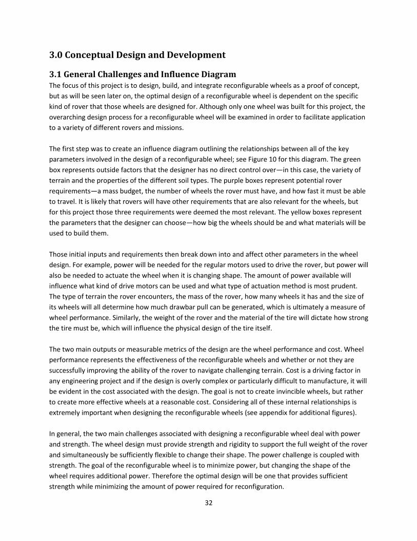
3.1 General Challenges and Influence Diagram The focus of this project is to design, build, and integrate reconfigurable wheels as a proof of concept,

but as will be seen later on, the optimal design of a reconfigurable wheel is dependent on the specific

kind of rover that those wheels are designed for. Although only one wheel was built for this project, the

overarching design process for a reconfigurable wheel will be examined in order to facilitate application

to a variety of different rovers and missions.

The first step was to create an influence diagram outlining the relationships between all of the key

parameters involved in the design of a reconfigurable wheel; see Figure 10 for this diagram. The green

box represents outside factors that the designer has no direct control over—in this case, the variety of

terrain and the properties of the different soil types. The purple boxes represent potential rover

requirements—a mass budget, the number of wheels the rover must have, and how fast it must be able

to travel. It is likely that rovers will have other requirements that are also relevant for the wheels, but

for this project those three requirements were deemed the most relevant. The yellow boxes represent

the parameters that the designer can choose—how big the wheels should be and what materials will be

used to build them.

Those initial inputs and requirements then break down into and affect other parameters in the wheel

design. For example, power will be needed for the regular motors used to drive the rover, but power will

also be needed to actuate the wheel when it is changing shape. The amount of power available will

influence what kind of drive motors can be used and what type of actuation method is most prudent.

The type of terrain the rover encounters, the mass of the rover, how many wheels it has and the size of

its wheels will all determine how much drawbar pull can be generated, which is ultimately a measure of

wheel performance. Similarly, the weight of the rover and the material of the tire will dictate how strong

the tire must be, which will influence the physical design of the tire itself.

The two main outputs or measurable metrics of the design are the wheel performance and cost. Wheel

performance represents the effectiveness of the reconfigurable wheels and whether or not they are

successfully improving the ability of the rover to navigate challenging terrain. Cost is a driving factor in

any engineering project and if the design is overly complex or particularly difficult to manufacture, it will

be evident in the cost associated with the design. The goal is not to create invincible wheels, but rather

to create more effective wheels at a reasonable cost. Considering all of these internal relationships is

extremely important when designing the reconfigurable wheels (see appendix for additional figures).

In general, the two main challenges associated with designing a reconfigurable wheel deal with power

and strength. The wheel design must provide strength and rigidity to support the full weight of the rover

and simultaneously be sufficiently flexible to change their shape. The power challenge is coupled with

strength. The goal of the reconfigurable wheel is to minimize power, but changing the shape of the

wheel requires additional power. Therefore the optimal design will be one that provides sufficient

strength while minimizing the amount of power required for reconfiguration.

33

Figure 10 - Influence Diagram

3.2 Three Different Wheel Designs Once all of the internal relationships were defined, the next step was to create feasible designs for the

wheels. The process began with general brainstorming regarding different shapes, materials, and

actuation methods. Some initial prototyping using cardboard, duct tape, thread, and wire ties was done

to test out design ideas. This initial prototyping helped to identify which concepts and ideas were

promising and which ones were obviously problematic. This brainstorming and prototyping resulted in

three main wheel designs that were subsequently modeled using the SolidWorks computer aided design

(CAD) system.

34

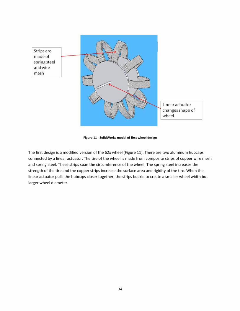
Figure 11 - SolidWorks model of first wheel design

The first design is a modified version of the 62x wheel (Figure 11). There are two aluminum hubcaps

connected by a linear actuator. The tire of the wheel is made from composite strips of copper wire mesh

and spring steel. These strips span the circumference of the wheel. The spring steel increases the

strength of the tire and the copper strips increase the surface area and rigidity of the tire. When the

linear actuator pulls the hubcaps closer together, the strips buckle to create a smaller wheel width but

larger wheel diameter.

35

Figure 12 - SolidWorks model of second wheel design

The second design, nicknamed the 3hubcap design, is essentially two narrow wheels connected as one

(Figure 12). There are three hubcaps connected to the linear actuator. As in the first design, when the

linear actuator pulls the hubcaps closer together, the strips buckle to create a smaller wheel width and

larger diameter. One of the major concerns with the first design was whether it would be strong enough

to support the weight of a large rover. The shorter composite strips in this design increase the strength

of the tire, making it less likely to collapse under larger loads.

36

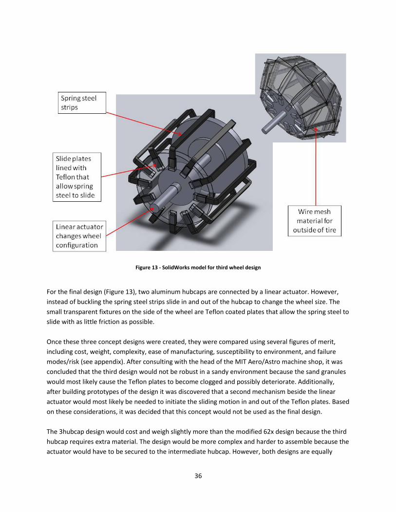
Figure 13 - SolidWorks model for third wheel design

For the final design (Figure 13), two aluminum hubcaps are connected by a linear actuator. However,

instead of buckling the spring steel strips slide in and out of the hubcap to change the wheel size. The

small transparent fixtures on the side of the wheel are Teflon coated plates that allow the spring steel to

slide with as little friction as possible.

Once these three concept designs were created, they were compared using several figures of merit,

including cost, weight, complexity, ease of manufacturing, susceptibility to environment, and failure

modes/risk (see appendix). After consulting with the head of the MIT Aero/Astro machine shop, it was

concluded that the third design would not be robust in a sandy environment because the sand granules

would most likely cause the Teflon plates to become clogged and possibly deteriorate. Additionally,

after building prototypes of the design it was discovered that a second mechanism beside the linear

actuator would most likely be needed to initiate the sliding motion in and out of the Teflon plates. Based

on these considerations, it was decided that this concept would not be used as the final design.

The 3hubcap design would cost and weigh slightly more than the modified 62x design because the third

hubcap requires extra material. The design would be more complex and harder to assemble because the

actuator would have to be secured to the intermediate hubcap. However, both designs are equally

37

susceptible to the environment and one design does not have significantly greater risk of failure than

the other. Therefore the most important comparisons between these two designs was how strong they

would be and how much force would be required for actuation. As mentioned previously, these are the

two key challenges in the wheel design. As such it was desirable to find a way to model and quantify

these two important parameters.

3.3 Wheel Sizing and Simulation Before computing the respective strengths of these designs it was necessary to determine the actual

dimensions of the wheel. The size of the wheel should obviously depend on the size of the rover, but it

should depend on other factors as well. Another important question to address for reconfigurable

wheels is what range of wheel size is most appropriate. The answer to this question is also dependent

on the type of soils the vehicle would navigate. One soil might require only a small change in wheel size

while another soil might require a much larger change in wheel size. There are so many different kinds

of soils that it would be impossible to design a reconfigurable wheel capable of traversing all types.

Since these wheels are for Mars rovers, a simulation was developed to examine the range of wheel sizes

needed for several different types of soil for a rover approximately the same size as Spirit and

Opportunity.

For this simulation, the terramechanic equations outlined in Equations 1-7 were used to compute

drawbar pull (DP) and torque (T) for five different types of soil and a range of wheel sizes. The objective

function developed by de Weck et al. (Equation 9) was also computed for each of these different soil

and wheel combinations. For each of the soil types, a minimum J point was identified at the point where

J was zero. A negative J could be caused by a negative DP value or by a DP value that was less than the

torque value. Since either situation is undesirable, the J = 0 point represents the minimum acceptable

wheel size. Graphical results of the simulation can be seen in Figures 14 and 15. The width in the

simulation ranged from 5 to 25 cm and the diameter ranged from 15 to 35 cm. The J value is

dimensionless because the DP and T values were normalized.

Figure 14 - Objective function graph for dry sand

38

Figure 15 - Objective function graph for sandy loam I

By identifying the J=0 boundaries for a variety of soil types, it was then possible to pick wheel

dimensions. In order to be effective in multiple soil types, the wheel needed to be capable of changing

its size to cross the J=0 boundary for as many soils as possible. Figure 16 shows J = 0 contours for

different types of soil and different alpha values. After running this simulation for five different soil types

whose soil properties were obtained from [10] and can be seen in Table 4, the maximum wheel width

was identified as 20.3 cm (8 in.) and the minimum wheel diameter was identified as 19.8 cm (7.8 in.).

Figure 16 - Graph of J=0 contours

39

Table 4 - Properties of Soils Used in Wheel Simulation

Soil Type kc [kN/mn+1] kφ [kN/mn+2] c [kPa] φ [deg] n K [m] Density [kg/m3]

LETE Sand 6.49 505.8 1.15 31.5 0.7 1.15 1600

Clayey Soil 13.19 692.15 4.14 13 0.5 1.15 1520

Sandy Loam I 2.79 141.11 15 25 0.3 1.13 1500

Dry Sand 0.99 1528.43 1.04 28 1.1 3 1600

Sandy Loam II 74.6 2080 0.22 33.1 1.1 2.54 1650

3.4 Strength Modeling (Deflection and Force) As can be seen from the influence diagram (Figure 10), one of the key relationships is the link between

the tire material and the actuators. The tire material dictates the strength of the tire. The tire strength

can be separated into axial and radial directions. The strength of the tire in the radial sense must be

strong enough to support the weight of the rover. The strength of the tire in the axial direction is

important because it dictates how much actuation force must be applied in order to change the shape of

the wheel. Greater force requirements also translate into greater power requirements, which must be

carefully monitored to fit within budget restrictions. Since both the axial and radial strengths are so vital

to the overall design and performance of the wheel, it was desirable to find a way to model them. For

the purposes of modeling, the tire strips were considered as individual components. The strength of

each strip was then calculated using simple beam theory. The weight of the rover acts downwards and

the natural tendency of the tire material will be to deflect under this weight. Therefore, the metric used

to evaluate the radial strength of the tire will be how much deflection occurs due to the weight of the

rover. A similar metric must also be used to evaluate the axial strength of the tire. When the hubcaps

are pushed together it causes the wire strips to buckle, therefore the metric used to measure axial

strength is the buckling force of the material. This is also a quantity that can be calculated from simple

beam theory [14].

Simple Beam Theory:

The equation from simple beam theory that describes the deflection in a beam is as follows:

(10)

w is the deflection, L is the length of the beam, q is the uniform load on the beam, E is the beam’s

modulus, and I is the beam’s inertia.

The equation for the buckling force is:

(11)

40

Pr is the buckling force and b1 is the length of the beam. An additional consideration that must be taken

into account for both equations is that the wire strips or “beams” are made of two different materials

that consequently must be modeled as composites. This requires that the overall material modulus be

weighted according to the relative area of the two materials and the overall material inertia must be the

combined inertia of both materials (Relevant material properties are listed in the appendix).

(12)

(13)

(14)

(15)

Table 5 - List of Variables for Equations 12–15

Symbol Variable

Ess spring steel modulus

Ecw copper wire modulus

Ass relative area of spring steel

Iss spring steel inertia

Icw copper wire inertia

b2 spring steel width

h1 spring steel thickness

A closed area of wire mesh

b3 wire mesh width

h2 wire mesh thickness

Simple Beam Theory Results

The length of the strips for the 62x design was 8.25 inches and the length of the strips for the 3hubcap

design was 4.5 inches. The width of the copper wire was 1.5 inches and the width of the spring steel was

0.25 inches. The buckling force required for two different spring steel thicknesses and two different wire

mesh densities can be seen in Tables 6 and 7.

Table 6 - Axial Strengths for Modified 62x Design

62x ver2 0.012” spring steel 0.015” spring steel

8 Mesh 12.91 N 13.30 N

10 Mesh 10.08 N 10.47 N

41

Table 7 - Axial Strengths for 3hubcap Design

3hubcap 0.012” spring steel 0.015” spring steel

8 Mesh 85.34 N 87.93 N

10 Mesh 66.67 N 69.22 N

To verify that these were reasonable results, a quick comparison was made with the initial 62x wheel.

That wheel was made from 10 Mesh copper wire and 0.012 inch spring steel. Both the spring steel and

the copper wire strips were 7 inches long. The actual wheel consisted of 16 composite strips and

required approximately 110 N of force to cause the strips to buckle. When the buckling force model is

run with the dimensions for the initial 62x wheel, the buckling force required for one strip is 14 N.

Multiplying that by 16 yields an estimated required buckling force of 224 N. There is about a 100 N

difference between the calculated buckling force and the actual buckling force. This shows that there is

room for improvement in the buckling model, so this model could only be used as a coarse first order

approximation. Since the main purpose of modeling the required buckling force is to have reasonable

force estimates with which the two different wheel designs can be compared rather than to exactly

determine the required buckling force, this simple beam model is sufficient for the purposes of model

comparison.

The buckling force estimates suggest that the density of the wire mesh has a greater effect on axial

strength than the thickness of the spring steel. More importantly, it can be seen that the 3hubcap design

requires approximately 6.5 times more buckling force than the modified 62x design. From a power

conservation standpoint, the 62x design is favorable over the 3hubcap design.

Thin Curved Beam Theory

As noted earlier, the metric used to evaluate the tire strength was the amount of deflection that would

occur in the tire material. Simple beam theory was initially used to compute this quantity. Equation 10

shows the deflection equation for simple beam theory. Deflection estimates made using this equation

yielded results that did not make sense since the deflection amounts were actually larger than the

length of the beam (see appendix). Therefore, another theory was found to more accurately model the

material deflection: thin curved beam theory [15]. This theory describes the deflection for a thin arch,

which is precisely what the tire material for the reconfigurable wheels is. Under this theory, the

deflection is given by:

(16)

(17)

(18)

42

Figure 17 - Pin supported arch for thin curved beam theory (Image courtesy of [15])

P is the load on the beam, R is the effective radius of the beam, α is the angle between the horizontal

surface and the pin location, and w is the amount of deflection (Figure 17). Using this theory to compute

estimates for the amount of deflection in the beam yielded much more reasonable results. For the 62x

design, the maximum deflection was 6.22 cm and for the 3hubcap design the maximum deflection was

0.54 cm. These numbers suggested that the 3hubcap design was significantly stronger than the 62x

design, which was not unexpected. In the 3hubcap design, each wheel is essentially two wheels, so the

weight of the rover was effectively distributed across eight wheels rather than only four. The effective

radius for this design is much smaller as well since the total width of a single wheel is essentially spread

across two wheels. So whereas the 62x design is more favorable than the 3hubcap design from a power

conservation perspective, the 3hubcap design is more favorable from a strength perspective.

3.5 Reconfigurability Metrics

While the concept of a reconfigurable wheel holds potential for improving a rover’s ability to traverse

challenging terrain, the idea is not without downsides. Additional power and hardware is required to

change the wheel’s shape and a reconfigurable wheel is certainly more complex than a non-

reconfigurable wheel. It is necessary to assess whether the net benefits from a reconfigurable wheel

outweigh the disadvantages. Siddiqi, de Weck, and Hoffman reviewed this concept of reconfigurability in

space systems and designed two important reconfigurability metrics to be used in determining whether

the net benefit of a particular reconfigurable system is positive or negative [16-17]. The first metric

defines a relative function efficiency (Ef) that compares the efficiency of the reconfigurable system to

the efficiency of a non-reconfigurable system whose capability is equivalent to the reconfigurable

system:

(19)

43

The functional efficiency of each system is defined as the ratio of the functional capability to the

resources required for that capability. The specific parameters that best quantify those metrics must be

individually defined for each system. For the reconfigurable wheels, it was decided that the functional

capability of the reconfigurable wheels was the ability to achieve multiple wheel states, and the

resource required to achieve that capability was the necessary wheel mass. In other words:

(20)

The functional efficiency of a non-reconfigurable wheel for a MER-sized rover was calculated. The

functional efficiency of a reconfigurable wheel for a similar sized rover with three wheel states was also

calculated. The relative functional efficiency (Ef) of this MER-sized system was 3.688. Any value greater

than one indicates that the reconfigurable system is favorable because it is more functionally efficient

than the non-reconfigurable system. In this case, the value is much greater than one, which suggests

that despite the need for additional resources, the reconfigurable wheels provide substantial functional

advantages over non-reconfigurable wheels.

The second reconfigurability metric defined by Siddiqi et al. was relative performance efficiency (Ep).

Similar to before, this metric compares the performance efficiency of a reconfigurable and non-

reconfigurable system.

(21)

Once more, the exact definition of performance efficiency is dependent on the particular application,

but in general the performance efficiency for each system is a ratio of performance to resources. For

reconfigurable wheels, the performance efficiency was defined as the ratio of the net drawbar pull of

each system (i.e. a performance metric) compared to the power required for each system (i.e., a

resources metric):

(22)

n represents the total number of states in the system. The relative performance efficiency was

calculated for the same reconfigurable, MER-sized system described above. Drawbar pull and power

values were averaged for five different soil types and calculated using Equations 1–8. The relative

performance efficiency for this system was 1.323. Again, this value is greater than one, which indicates

that the reconfigurable system provides a net gain in performance. Hence, the results from both

reconfigurability metrics suggest that there is a net benefit in using reconfigurable wheels for planetary

rovers.

44

3.6 Design Selection At this point, it has been quantitatively shown that using either the 3hubcap reconfigurable wheels or

the 62x reconfigurable wheels is more efficient than using non-reconfigurable wheels. The 3hubcap

design and the 62x design have both been analyzed and compared according to cost, weight,

complexity, ease of manufacturing, susceptibility to environment, failure modes/risk, and strength. As

explained earlier, strength is the most critical figure of merit. For the specific case of a MER-sized wheel,

the best design choice is the 3hubcap design. This design requires more force to actuate (i.e., more axial

strength), but its radial strength is significantly greater. The radial strength is more important than the

axial strength because the primary requirement of the wheel is that it is capable of supporting the

weight of the rover.

From the analysis it is also possible to make design selections in a more general sense. As robotic

exploration expands, rovers will undoubtedly be used more extensively and there will be many different

sizes of rovers needed. The results presented in this section were all based on using a MER-sized rover

model, but it is hoped that the software tools developed here will aid in the design of reconfigurable

wheels for other rover sizes as well, since it is possible to change the rover size in the simulation codes.

While the 3hubcap design is the optimal choice for a MER-sized rover, it is important to note that the

62x design would be sufficiently strong to support the weight of smaller rovers. Based on the analysis

completed in this project, for smaller rovers (i.e., < 25 kg) the 62x reconfigurable wheel design would be

recommended because it provides sufficient strength while minimizing power, but for larger rovers

(such as MER-type rovers) the 3hubcap reconfigurable wheel design is the best choice to ensure

sufficient wheel strength.

45

4.0 Fabrication and Assembly

4.1 Rover Platform Selection Once the design analysis had been completed, the next step was to make material and part selections.

The first part selection regarded which rover platform the wheels would be installed on. Originally it was

hoped that the K-REX rover from ProtoInnovations would be available for use. The K-REX rover is an

actual rover used for earth-based rover testing. Unfortunately, the K-REX rover could not be used due to

some legal issues so it became necessary to find an alternative rover platform. Several options were

considered. The most promising options were a large RC “monster truck”, a child’s ride-on electric car,

or a VEX robot. After weighing the pros and cons of these different options, the VEX robot was selected

as the rover platform (Figure 18). Although significantly smaller than a MER type platform, this platform

could be purchased as part of a kit that included drive motors, a microcontroller, and a number of

different sensors—all necessary items to make the rover autonomous. The rover base is approximately

7.5 inches wide and 12.5 inches long. The rover came with 5 inch diameter wheels, but rather than using

these wheels, the reconfigurable wheels were attached to the rover platform instead. The size of this

rover platform was comparable to the Sojourner rover, and its mass was within the small rover category,

therefore the modified 62x wheels were the best design choice for this platform.

Figure 18 - VEX Robot

4.2 Material and Part Selection Once the wheel design and rover platform were chosen, the details of the wheel size and type of

materials could be determined. Since the purchased robot was about the same size as the Sojourner

rover, the wheels were sized similar to the Sojourner wheels. The hubcaps were 4.5 inches in diameter

and the tire strips were 6.5 inches long. After assembly, the minimum wheel width was 2.75 inches and

the corresponding maximum diameter was 8.75 inches. The maximum wheel width was 3.75 inches and

the corresponding minimum diameter was 8.5 inches.

46

Hardened (spring tempered) spring steel and a copper wire mesh were used for the tire strips. The

spring steel had a thickness of 0.012 inches, a width of 0.25 inches, and a length of 6.5 inches. The spring

steel strips were cut using a waterjet cutting machine. The copper wire mesh was made from 0.025 inch

diameter copper wire and had a 10 mesh density (i.e. 10 x 10 mesh/square inch). This thickness for the

spring steel and density for the copper wiring were chosen because both provided the best balance

between flexibility and strength. The copper strips were 1 inch wide and 6.5 inches long. The copper

mesh came in a large sheet so the strips were cut by hand using heavy-duty cutting shears. The spring

steel strips were centered on the copper mesh strips and hand-sewn together using steel wire (Figure

19). Each wheel had thirteen tire strips.

Figure 19 - Composite tire strips made from spring steel and copper mesh

The hubcaps were made out of aluminum. This material was chosen because it is light-weight and cost

effective, and the Aero/Astro machine shop has the proper tools needed for cutting and shaping it. The

outer hubcaps were 0.125 inches thick and the inner hubcaps were 0.1875 inches thick. The inner

hubcap was slightly thicker because the actuator was mounted to this hubcap; having a slightly thicker

hubcap permitted deeper screw holes and a more secure mounting. In order to attach the tire strips to

the hubcaps, a ring flange was made to go along with each hubcap. The ring flanges were also made out

of 0.125 inch thick aluminum. Eight evenly-spaced holes were drilled and tapped into the hubcaps. Eight

corresponding clearance holes were drilled in the ring flanges so the flanges and hubcaps could be

screwed together (Figure 20). The tire strips were secured to the hubcaps by placing them in between

the hubcap and ring flange and screwing the hubcap and ring flange together as tightly as possible.

47

Figure 20 - Aluminum hubcap and ring flange

The biggest challenge in selecting the parts was finding an acceptable linear actuator. A very extensive

on-line search was conducted, but most available linear actuators were either not strong enough or

lacked the needed range of motion. Another problem was finding cost effective actuators that would fit

within the limited budget of this project. In the end, the only actuator that provided enough strength, fit

within the budget, and had an adequate range of motion was a linear actuator from a company called

Anaheim Automation. This actuator consists of a stepper motor and leadscrew (Figure 21). The motor

screws the leadscrew in and out creating a translational motion. The range of available travel for the

actuator is 4.5 inches and it is capable of exerting 24 lbs of force.

Figure 21 - Linear actuator used in reconfigurable wheel

4.3 Wheels and Platform Integration After the parts and materials were selected and acquired, the next step was to determine the details of

the rover/wheel integration. The integration design presented several challenges, especially in regard to

the linear actuator. As discussed above, the linear actuator was mounted to the inside of the hubcap

closest to the rover frame (i.e., the inner hubcap). A hole was drilled through the center of the hubcap

to allow room for the leadscrew to pass through. The outer hubcap also had a hole drilled in its center

48

through which the other end of the actuator leadscrew emerged. This end of the leadscrew was

attached to the outer hubcap by placing a collar on both sides of the hubcap. When the wheel was in its

largest width configuration, the leadscrew for the actuator would sit entirely on the inside of the wheel,

but when the actuator pulled the hubcaps together, the leadscrew would extend outside the wheel. This

meant that the wheel needed to be offset approximately 3 inches from the rover frame. The wheel axle

also needed to be longer and avoid interfering with the leadscrew. It was decided that a hollow tube

would be attached to the outside of the inner hubcap to provide a protective case for the leadscrew and

extend the length of the wheel axle (Figure 22). In order to attach the hollow tube to the hubcap, the

hubcap needed to have a built-in flange. This element of the design was accomplished by turning a solid

piece of aluminum on a lathe to create the inner hubcaps; the outside hubcaps did not require a flange

and were cut using the waterjet.

Figure 22 - Wheel Attachment Design

The hubcaps were 4.5 inches in diameter. The outer hubcap was 0.125 inches thick and the inner

hubcap was 0.1875 inches thick. The flange for the inner hubcap was 0.375 inches thick and 0.875 inches

in diameter. The axles for the wheels and drive motors that came with the robot kit were 0.125 inch

square axles, so in order to use these drive motors, it was necessary to also use 0.125 inch square axles.

The outer diameter of the tube was 1 inch, thus a tapered aluminum plug was made to gradually

decrease the size of the axle. The 0.125 inch axle was made out of steel stock and press fitted into the

aluminum plug. The hollow tube was pinned to the flange on the hubcap and the aluminum plug was

pinned to the tube (Figure 23).

leadscrew

linear actuator

collar hollow tube

inner hubcap

outer hubcap

49

Figure 23 - Wheel axle attachment

The next major integration issue that was addressed was related to electrical wiring. Since the stepper

motor was on the inside of the hubcap it rotated with the wheel. This presented a problem because the

electrical wires that powered the stepper motor got tangled as they also rotated with the wheel. One of

the technical instructors suggested that an electrical slip ring could be used to solve this problem. Price

quotes from several companies were obtained for electrical slip rings, but the prices were outside the

budget range for this project. Therefore it was decided that the slip rings would be manufactured

instead.

A company was identified that sold PCBs (printed circuit boards) which are very thin copper sheets with

a composite laminate on the bottom. The plan was to cut concentric circles out of this material using the

waterjet and then epoxy the circles onto the outside of the inner hubcap (Figure 24). The stepper motor

has four wires so four circles were needed. For each wire, a small hole was drilled through the hubcap

and the wire was fed through this hole and then soldered to one of the copper rings on the outside of

the hubcap. Small metal brushes then sat against the copper circles

with the wheel (and stepper motor wires) free to rotate. Wires

were soldered to the brushes, which maintained constant contact

with the copper circles and provided a pathway whereby electrical

signals could be sent from outside to inside the wheel (Figure 25).

Some experimentation was required to figure out what size the

circles should be and what settings should be used for the waterjet

when cutting the PCB material. The material tended to delaminate

under normal settings so low pressure and very brittle material

settings had to be used instead. The metal brushes were made from

RFI EMI shielding gasket fingers from a company called

OmegaShielding. This was not the most robust design—the brushes

aluminum plug

axle made from

steel stock

hollow tube and hubcap

flange pinned here

aluminum plug and hollow

tube will be pressed and

pinned together here

Figure 24 - Copper electric slip rings mounted to outside of inner hubcap

50

were not expected to withstand extended periods of use—but the total cost for these slip rings was only

about $20 and cost was the driving factor for this design. The slip rings successfully worked the first time

they were tested and have performed well for the duration of this project. These slip rings are

sufficiently robust for demonstrating a proof of concept; however, a real rover would probably need

more robust parts (See appendix for a list of major parts, dimensional drawings, and hardware

specification sheets).

Figure 25 - Wire brushes for slip rings

4.4 Assembly Assembling the wheel after manufacturing was completed was not an easy task. It was critical to do

some tasks in a specific order. Before assembly, the following tasks were completed first:

1. Cut spring steel strips using the waterjet and cut copper strips using cutting shears.

2. Sew spring steel strips and copper strips together using steel wire.

3. Cut outer hubcap and ring flanges using the waterjet.

4. Make inner hubcap using a lathe.

5. For the outer hubcap, drill a center hole that actuator leadscrew can fit through, and drill and tap

eight evenly spaced holes around the outer edge.

6. For hubcap rings, drill eight evenly spaced clearance bolt holes around the outer edge.

7. For the inner hubcap, drill center hole for leadscrew, drill and tap mounting holes for actuator, drill

clearance holes for actuator wires, and drill and tap eight evenly spaced holes around the outer

edge.

8. Cut hollow steel tube that will extend wheel axle and enclose actuator leadscrew.

wire brush for slip rings

51

9. Make tapered aluminum plug for connecting wheel axle to steel tube using a lathe.

10. Drill starter hole for wheel axle into tapered plug.

11. Cut wheel axle from steel stock.

12. Cut electrical slip rings using the waterjet.

The above items do not necessarily have to be performed in that order. After all the tasks have been

completed, the wheel is ready to be assembled by completing the following steps in the order listed:

1. Press outer hubcap onto one end of steel tube.

2. Drill two 0.0625 inch holes through steel tube and aluminum hubcap (holes should be 180 degrees

apart).

3. Hammer spring-loaded pins into holes (this task may require two people).

4. Install grommets in wire holes for outer hubcap.

5. Epoxy electric slip rings onto outside edge of inner hubcap with copper side up. Allow 24 hours for

epoxy to dry.

6. Press fit wheel axle into tapered plug.

7. Press tapered aluminum plug into open end of steel tube and then drill two 0.0625 holes through

steel tube and aluminum plug (holes should be 180 degrees apart).

8. Hammer spring-loaded pins into holes (this task may require two people).

9. Once epoxy has dried, mount actuator to inside of inner hubcap and then thread actuator wires

through wire holes.

10. Place ring flange on the inside of inner hubcap and attach to hubcap by loosely screwing together.

11. Evenly space 13 tire strips around inner hubcap. The strips should sit in between the hubcap and

ring flange.

12. Once all the strips are in place, tighten all screws. This is best done by tightening screws gradually

in a star pattern similar to tightening lug nuts on a tire.

13. Attach outer hubcap to leadscrew by securing it between two collar attachments.

14. If necessary, screw in leadscrew so that only 2.5–3.0 inches are exposed.

15. Place ring flange on the outside of outer hubcap and attach to hubcap by loosely screwing them

together.

16. Gently bend each tire strip and place the free end in between the outer hubcap and its ring flange.

17. Once all strips are in place, gradually tighten all screws again following a star pattern.

18. Solder actuator wires to the tabs on the electrical slip rings.

Figures 26-29 show various steps in the assembly process. It should be noted that it can take several

hours to assemble one wheel. For some of the steps it is helpful to have another person available to

assist in holding and securing parts. In particular, getting all the tire strips correctly situated can be an

arduous task and will likely take several attempts and some patience to accomplish.

Initially, only one wheel was built and assembled. This attempt was a trial-and-error experiment that

allowed me to learn how to use all the machines necessary to make the parts, what order to assemble

things in, and decide if any size adjustments were necessary for the individual pieces. Once the first

wheel was successfully built and the fabrication and assembly process was “de-bugged,” three more

52

wheels were built. Once all four wheels were assembled, they were attached to the rover platform (i.e.,

the wheel axles were secured in the shafts of the drive motors) and the rover was ready for its first test

drive.

Figure 26 - Wheel axle, hollow tube, and inner hubcap all pinned together

Figure 27 - Linear actuator mounted to inner hubcap

53

Figure 28 - Securing the tire strips

Figure 29 - The first assembled wheel

4.5 Initial Drive Testing After the assembly was complete, some initial drive tests were conducted to verify that the wheels

could support the weight of the rover. During the initial tests, there was a large bending moment

54

occurring at the wheel axles because they were situated so far from the rover frame. The fact that the

wheel axles were small compared to the wheels also exacerbated this problem. After several initial

driving tests, the axles on one of the wheels broke off. In order to fix the broken wheel, a new axle was

cut, the old aluminum plug was cut off of the steel tube, a new aluminum plug was turned on the lathe,

the new plug had to be pinned to the steel tube, and the new axle had to be pressed into the new plug.

To provide more structural support and prevent more broken axles in the future, support bars were

designed and built to take some of the stress off the axles. There was one bar for the front wheels and

one bar for the back wheels. Both bars were cut from 0.25 inch thick aluminum stock. They were 14.5

inches long and 2.0 inches wide. Clearance bolt holes were drilled into the support bars and then offsets

were used to attach the bars to the frame. Bearings were needed to attach the bars to the wheels. Small

mounts with holes for the bearings were cut out of aluminum using the waterjet and the bearings were

pressed into the mounts. The steel tubes sat inside the bearings and then the bearing mount was

screwed into the support arms (Figure 30). Additional drive testing conducted after the support arms

were built demonstrated that they were able to resolve the bending moment issues.

Figure 30 - Rover with four reconfigurable wheels and support bars

One other minor issue was identified during the initial drive testing. Because of the are gaps between

the tire strips and the holes in the copper mesh itself, if the rover was driving on sand or some other

loose, dusty terrain, small soil particles would sometimes get stuck in the leadscrew and motor gears. To

protect against soil and dust contamination, covers for the wheels were sewn using a sewing machine.

The covers were made out of spandex in order to stretch and conform to the shape of the wheel as it

changed to different configurations (Figure 31). Different patterns were experimented with until finally

one was made that matched the contour of the tire strips.

horizontal support bars

mounts and bearings

55

Figure 31 - Wheel with hand-sewn spandex cover

56

5.0 Integration, Autonomy, and Control

5.1 Electrical System Overview At this point, the project objectives to build four reconfigurable wheels and integrate them onto a rover

platform were complete. The next goal was to demonstrate that the wheels could autonomously

reconfigure. This required a working electrical system, and eventually that the mechanical and electrical

systems be integrated to successfully work together. The electrical system for the rover can be

considered as two subsystems. One subsystem is responsible for controlling the wheel as it drives and

the other subsystem is responsible for reconfiguring the wheels. The wheels are independently driven so

each wheel requires its own drive motor. The drive motors are controlled by a microcontroller, though

initially the drivers were tested independent of each other using power supplies and a signal generator.

This was done to test out the wheels and stepper motors, and to ensure proper usage.

The drive motors and their accompanying microcontroller were included in the robotics kit that was

purchased for the rover platform. The microcontroller came with built-in ports designed specifically for

the drive motors. Once plugged in, their power setting could be controlled via the microcontroller.

Eventually the drivers would need to be powered by batteries and the microcontroller. The

microcontroller had its own battery, but the drivers needed their own power source. The reconfigurable

wheels were much larger (in both size and weight) than the wheels that came with the robot kit, so it

was necessary to find the minimum power required for the rover to drive forward using the

reconfigurable wheels. Through experimentation, it was discovered that the minimum power setting

was 40% on a hard floor.

Controlling the stepper motors (i.e. linear actuators) used to reconfigure the wheels is more challenging

than controlling the drive motors. A driver is required to interface between the stepper motor and the

microcontroller. The stepper motor’s shaft is a permanent magnet surrounded by electromagnets. The

shaft is turned by energizing the electromagnets in a specific pattern. If given direction and speed

commands, the motor driver will translate those commands into the appropriate input signals to power

the electromagnets. The direction command is either hi (1) or lo (0). To control the speed, the driver

must receive a square pulse. The higher the frequency of the pulse, the faster the stepper motors will

turn (see appendix for more details).

5.2 System Integration and Preliminary Testing The first step in the integration process was learning to program the microcontroller. This was a trial-

and-error process. The microcontroller had a number of digital input/output pins (I/O pins) capable of

receiving or sending either hi signals (1) or lo signals (0). A lo signal causes the linear actuator (i.e.,

stepper motor) to pull the hubcaps together while a hi signal pushes the hubcaps apart. The square

pulse is generated by pulling the same pin lo and then hi. There is a programmed time delay in between

the lo and hi commands. The frequency of the square pulse can be altered by changing the length of this

time delay. A program was written to generate a square pulse and the output was verified by hooking

up the microcontroller to an oscilloscope.

57

Once the driver could be controlled using the microcontroller and powered using batteries, initial

reconfiguration testing was conducted. The initial testing was, in short, unsuccessful due to two main

problems. The first problem was mechanical in nature. The correct signals were being sent to the drivers

and the stepper motors would turn, but the leadscrew struggled to move in or out. After

troubleshooting, it was observed that when the wheels supported the entire weight of the rover, the

hubcaps became misaligned. Since the hubcaps are attached solely by the linear actuator, it plays both a

structural role and a dynamic role. Although the linear actuator can provide enough force to actuate the

wheel, it cannot provide sufficient structural support. The misalignment of the hubcaps caused the

leadscrew to sit at an angle to the motor which was not powerful enough to overcome the misalignment

and still turn the screw.

If the hubcaps were supported by me, however, the wheel would successfully reconfigure. Given this

observation, it was clear that either manual intervention would be necessary during the testing or

additional support structures would be required to fix the misalignment. After consulting with the

project advisor, it was decided that demonstrating the autonomy of the wheel warranted that additional

support structures should be built. Designing these support structures was difficult because it required

supporting the outside hubcap. Since the outside hubcap moves when the wheel reconfigures, the

support structure would need to move along with it. Additionally, the support structure must require

little or no power to move or else the linear actuators may not be able to move the hubcaps and the

supports.

After brainstorming, the project mentor suggested the use of (nearly) frictionless rails. The rails would

be mounted to the rover’s frame. Support arches could then be built that would attach to the outside

hubcaps at one end and the rails on the other end. The arches would keep the hubcaps aligned and the

rails would allow the arches to move back and forth with minimal additional power. Similar to the

support arms previously made, bearings and bearing mounts were needed to attach the arches to the

hubcaps. Special bearings capable of withstanding both radial and axial loads were purchased and new

collars were custom made on the lathe to fit inside the bearings (Figure 32). The support arches and

additional aluminum bearing mounts were designed and cut using the waterjet. The bearings were

glued into the mounts using Loctite adhesive (Figure 33), and bolt holes were drilled and tapped into the

ends of the support arches so that they could be screwed together with the bearing mounts. The

frictionless rails were screwed to the horizontal support arms, with specially designed carts that could

slide back and forth with relative ease (Figure 34). The support arches were mounted to these carts and

then they extended over the tops of the wheels where they met the bearing mounts (Figures 35–37).

Care was taken when making measurements for these new pieces to ensure that each remained

properly aligned. Designing these support arms was an involved process, but after they were

implemented, the actuator leadscrew misalignments were no longer a problem.

58

Figure 32 - Custom made collar to connect leadscrew, bearing/mounts, and hubcaps

Figure 33 - Bearing and bearing mount for support arch

bearing

bearing mount

59

Figure 34 - Frictionless rails mounted to rover frame

Figure 35 - Rover with new support arches

frictionless rail rail cart

support arches

60

Figure 36 - Close-up of rail, cart, and arch

Figure 37 - Close-up of new hubcap attachment

The second major problem during the initial reconfiguration testing happened while troubleshooting the

misalignment problem. It is not known exactly when or why this happened, but at some point the

drivers for the stepper motors burned out and stopped working. There did not seem to be any major

electronic malfunction so it was hypothesized that the drivers, which were fairly low quality, were too

small or inefficient to power the motors. Some higher-quality drivers were purchased, but installing

them required that all the electrical connections be re-done. These new drivers were also significantly

more expensive than the previous drivers, so in an effort to save money only two drivers were

support arch

frictionless rail

rail cart

support arm

bearing

bearing mount

61

purchased and each driver was connected to two wheels. According to all the product specifications this

should have been a viable option, but the new drivers exploded on the first testing attempt after they

were installed (Figure 38). It is still not understood what caused this malfunction. New, even more

heavy-duty drivers were again bought, and in an effort to avoid destroying any more motor drivers, it

was decided that each wheel would have its own driver. These new drivers were incrementally tested

and set-up. After a labor-intensive effort and a third re-work of the electrical system, the rover finally

had four working drivers to go along with its wheels.

Figure 38 - Charred remains of a motor driver after it exploded

Unfortunately this was not the end of the electrical system problems. The drivers and motors could

successfully operate off of a signal generator, but when the microcontroller was hooked up instead the

drivers (and hence the motors) stopped working. After another painstaking troubleshooting procedure it

was discovered that the new drivers operated on a 5V electrical standard, but the microcontroller

operated on a 3.3V standard. The new motor drivers were therefore incompatible with the

microcontroller. Some small translator chips were bought, but this too ended in failure because even

with the translator chips, the microcontroller was incapable of producing the amount of current

required for the drivers. It was decided that the easiest solution was to use a different microcontroller

for reconfiguring the wheels. The Arduino Uno, a small microcontroller that operates on a 5V standard,

was obtained, programmed, and successfully used to reconfigure the wheels (see appendix for detailed

diagram of the electrical set-up).

5.3 Control Methodology With working mechanical and electrical systems, the final issue to address was determining how the

rover would decide when it needed to reconfigure. Designing the optimal control algorithm for this is an

62

entire project in itself. Several researchers have developed in-depth control strategies for identifying

and controlling wheel slip and traction [18-19]. The purpose of this project was not to optimize a control

strategy for a rover with reconfigurable wheels, but a working control algorithm was necessary to

demonstrate the autonomous capability of the rover. Time limitations permitted only a very simple

control algorithm to be developed. While the reconfigurable wheels were being built, initial testing with

the wheels that came with the robot kit was being conducted on various terrains to investigate what

happens prior to the rover getting stuck. Video was taken of the rover in these different terrains and the

film was studied as part of the control algorithm development process. It was observed that the most

likely indicator of the rover becoming stuck was wheel slip. Therefore, wheel slip was selected as the

event that would be measured and used to indicate when the wheels should reconfigure.

Wheel slip occurs when a wheel is rotating but the rotation fails to move the vehicle forward. In most

cases, not all the wheels begin to slip at the same time, so an easy way to detect wheel slip is by

measuring and comparing the rotation rates of two or more wheels. If the rotation rates are not the

same, then wheel slip is beginning. Although the rover wheels are all independently driven, the front

wheels and back wheels still tend to work in pairs, similar to cars operating on rear wheel drive. Because

the two back wheels pull together and the two front wheels pull together, the best way to detect wheel

slippage is by comparing the front wheels to each other and the back wheels to each other (as opposed

to comparing the right wheels to each other and the left wheels to each other).

Rotation rates can be measured using simple sensors called encoders. Two such sensors were purchased

and installed on the back wheels of the rover. While comparing both sets of wheels is likely more

optimal than comparing only one set of wheels, the project’s need for an effective yet simple control

algorithm could be met with just one comparison. From a software engineering perspective, writing a

program to compare two sets of wheels is more complex than one to compare just one set of wheels.

The back wheels were chosen for comparison because in the preliminary testing they tended to get

stuck more often than the front wheels. The algorithm was programmed to have the encoders

continuously measure the rotation rates of the wheels as the rover drove forward. The rotation rate

information would be sent to the microcontroller, which would continuously compare the rotation

rates. If the rates differed too much, the microcontroller would stop the rover because it would mean

the wheels were slipping and needed to be reconfigured to improve traction (Figure 39).

63

Figure 39 - Flowchart for reconfiguration control algorithm

5.4 A Systems Engineering Perspective With the control algorithm completed, it was time to enter the testing phase of the project. Before

doing so, however, it is worthwhile to make a few closing comments about the rover itself. As this

project progressed from the initial design and building phases into the integration phases it became

clear that this project was indeed a systems engineering project. There were certainly design and

fabrication challenges, but the greatest difficulties in this project were associated with integrating all of

the mechanical, electrical, and software systems together. These subsystems could not be thought of as

individual entities; rather design decisions for one system had to also consider the effects on the other

subsystems. An outstanding subsystem is useless if it is incompatible with the system at-large. A design

structure matrix shown in Figure 40 diagrams the different interactions that exist between different

components of the rover system. Black boxes indicate structural connections, green boxes indicate

signal flows, and red boxes indicate energy flows.

64

Figure 40 - Design structure matrix for rover system

Some of the biggest mistakes made during the course of the project related to integration. At first,

everything was assembled all in one step, but this strategy only resulted in things not working or in the

most extreme cases, exploding. One of the most significant lessons learned from this project was that

the key to successful integration is taking small, incremental steps. A system is made from many

different components, and it must be built and tested one component at a time. Systems engineering is

a delicate balancing act that requires a focus on the subsystems while simultaneously maintaining a view

of the entire system. In order to achieve that balance with the rover, it had to be thought of as a system.

The individual components of subsystems had to work correctly, but the sub-systems themselves also

had to be thought of as components that must be compatible with each other. Issues related to mass,

power, design, performance, and cost all had to be considered from the perspective of the entire rover,

not just a particular subsystem.

During the course of development, this project demonstrated that even small problems or changes

within a subsystem can have rippling effects. For example, the choice to use linear actuators for

reconfiguration affected not only the mechanical design of the system but also the electrical design of

the system by requiring the use of slip rings and microcontrollers. The failure to anticipate bending

Bat

tery

(NiM

H)

Ard

uin

o

Mic

roco

nt

rolle

rH

ori

zon

tal

Sup

po

rt

Bar

s

Rai

ls

Sup

po

rt

Arc

hes

Enco

der

s

Bat

tery

(LiP

o)

Wh

eel

Axl

e

Ro

ver

Fram

e

Act

uat

or

Dri

vers

Dri

ve

Mo

tors

VEX

Mic

roco

nt

rolle

r

Battery (LiPo)

Battery (NiMH)

Arduino

Microcontroller

Horizontal Support

Bars

VEX Microcontroller

Actuator

Drivers

Drive Motors

Rails

Support Arches

Encoders

Wheel

Axle

Rover Frame

65

moment problems led to a series of design add-ons, increased costs, and as will be seen later, changes

to the testing environment and procedure. Similarly, issues with the original motor drivers eventually

led to incompatibilities within other aspects of the electrical system and required several redesigns.

As the engineering world takes on greater challenges and as systems become increasingly complex, it is

imperative to understand engineering from a systems perspective as well as a micro fluidic or resistor

and transistor perspectives. Similar to an orchestra conductor who must be aware of individual

instruments while also creating a symphonic whole, engineers must pay attention to individual

components while also ensuring that all subsystems are working in harmony to create an engineering

masterpiece.

66

6.0 Testing and Results

6.1 Test Set-Up In order to demonstrate and assess the effectiveness of autonomous reconfigurability, it was necessary

to create a Mars-like environment for the rover, which is non-trivial. The natural choice for a Mars-like

soil is sand, but using sand was very risky because the rails that were added to keep the wheel hubcaps

aligned are very sensitive to sand and dust. In order to maintain their nearly frictionless state, the rails

must be kept free of sand and dust. If the rails were to become contaminated, the autonomous

reconfigurable capability of the rover would be compromised. Considering the project time constraints

and the high risks associated with testing in sand, it was decided that sand should be strictly avoided.

However, it was still desirable to use a material that would mimic the behavior of sand.

The first sand replacement material that was tried was pea gravel. A “sandbox” three feet wide, ten feet

long, and three inches deep was constructed out of plywood. The box was filled with 500 pounds of fine-

grained pea gravel purchased from a home improvement store. Several test drives with the rover were

conducted in the gravel but no slippage was occurring. As a result, it was decided that the pea gravel

would not be a suitable substitute for sand. Two more materials were experimented with—rice and

popcorn seeds. These may sound like odd materials to use as sand substitutes, but keep in mind that the

main goal of the test set-up was not to exactly replicate the Martian surface, but rather to simulate a

Mars-like environment where the rover would likely slip due to the nature of the terrain. The rice and

popcorn simulate a sand-like environment in that both consist of small grains that can easily slide

against each other. As it would in sand, the rover tended to sink into the rice, but the sinkage was not

deep enough that the rover ever lost traction. The popcorn seeds, however, were much more

successful. Prior to testing in the alternative soils, testing had been conducted to calibrate how much

wheel slippage occurred on a flat solid floor. This amount of slippage was designated as a normal or

acceptable level. In the alternative soils, the rover was commanded to drive forward but stop if it

detected that the wheel slippage became greater than the acceptable amount. The rover experienced

above average slippage in the popcorn seeds, therefore it was decided that these would be the material

of choice for the homemade Mars yard (Figure 41).

67

Figure 41 - Testing in the homemade Mars yard filled with pea gravel and popcorn

6.2 Testing Procedure The purpose of the testing was to fulfill the last two objectives of the project, namely, to demonstrate

the ability of the rover to autonomously reconfigure its wheels and to assess the effectiveness of using

reconfigurable wheels in a simulated Martian environment. The first objective was documented via

video. To fulfill the second and final objective, data for the reconfigurable wheels was collected by

recording relevant measurements as part of the testing.

Recall that the basic motivation behind designing a reconfigurable wheel was to find a better trade-off

between the competing metrics of drawbar pull and power. Measuring drawbar pull is very difficult, but

in this case a related metric is distance. If the rover gets stuck it will not travel very far; with the aid of

reconfigurable wheels the rover will be able to travel greater distances in challenging terrain. Given this,

the first measurement that was collected in the tests is the distance traveled by the rover. The second

measurement that was collected is power. The distance was measured using a measuring tape. The

amount of current used to drive the motors was also measured and then multiplied by the battery

voltage to calculate power. The tests were conducted using different rover speeds (slow vs. fast),

inclinations (flat vs. tilted), and terrain types (easy/flat vs. hard/bumpy). Results using the reconfigurable

wheels were compared against results without reconfiguring the wheels. In the non-reconfigurable

system testing, the wheels began in the smallest width configuration and the rover drove as far forward

as it could before it exceeded slippage limits described earlier. For the reconfigurable system testing, the

wheels again began in the smallest width configuration. Once the rover exceeded its slippage limits, the

wheels were allowed to reconfigure to the largest width configuration and the rover continued driving

68

forward until it again exceeded its slippage limit, hence the tests only focused on reconfiguration from

smallest to largest width. A copy of the test procedure can be viewed in the appendix. Figure 42 is a test

matrix that outlines all the different tests that were conducted. A slow speed meant that the motor

power was set at 70% and a fast speed meant it was set at 80%. For the inclined scenarios, the far end of

the test bed was raised up by two inches. The easy terrain scenario meant that the surface was flat. For

the hard terrain scenario, small craters were manually introduced to the test environment to create a

bumpy surface. Five tests were conducted in each test scenario with the exception of the fast speed/no

tilt/easy terrain scenario. For that scenario, a set of 25 tests was done so that a larger sample size would

be available to conduct an error analysis. For each scenario, the results from the individual tests were

averaged together. These results are discussed in the next section.

Figure 42 - Text matrix of testing procedures

6.3 Test Results The first metric that was examined was the average distance achieved using the reconfigurable wheels

for each of the test scenarios. These results can be seen in Figure 43. The slow, bumpy, tilted scenario

had the smallest distance and the fast, easy, no tilt scenario had the largest. These results are not

surprising. An inclined surface and a bumpy surface both create additional soil resistances, which

impede the progress of the rover. Additionally, a rover moving at faster speeds will have more

momentum which can assist in navigating the terrain. It is interesting to rank the different scenarios

according to their distance achieved. From smallest to largest, the order is:

1) slow, bumpy, tilted

2) slow, bumpy, no tilt

3) fast, bumpy, tilted

4) fast, bumpy, no tilt

5) slow, easy, tilted

6) slow, easy, no tilt

7) fast, easy, tilted

8) fast, easy, no tilt

This ranking can be further divided into three distinct groups: small distances (scenarios 1 and 2),

medium distances (scenarios 3–5), and large distances (scenarios 6–8). It is interesting to note that the

69

common characteristic of the high distance group is the easy terrain which suggests that distance was

most heavily influenced by terrain difficulty. Further examination of the ranking suggests that the next

most influential factor was speed and inclination was the least influential factor.

Performing similar analysis from a different data perspective is also revealing. The difference between

the distance achieved by the non-reconfigurable system and the distance achieved by the reconfigurable

system was also examined. Figure 44 outlines the additional distance achieved in each test scenario

thanks to the reconfigurable wheels. The ranking of these scenarios, again from lowest to highest, is as

follows:

1) slow, bumpy, tilted

2) slow, bumpy, no tilt

3) slow, easy, tilted

4) fast, easy, tilted

5) fast, bumpy, tilted

6) fast, bumpy, no tilt

7) slow, easy, no tilt

8) fast, easy, no tilt

In this case, the larger distance is grouped by speed more than terrain. The most likely explanation for

this is that for the reconfigurable system, the rover has more trouble restarting after it has reconfigured

its wheels than when it is first starting. When the rover initially begins to move forward it has good

flotation over the surface. However, as it moves forward the sinkage of the rover increases. The rover

stops to reconfigure its wheels after it has started to get stuck in the soil, so when the rover attempts to

drive forward again after reconfiguring its wheels, it must now overcome not only its natural inertia but

the additional resistance due to more sinkage. Since a higher speed translates into more power, the

rover is more capable of overcoming the additional resistances and traveling farther distances when

moving at a higher speed.

70

Figure 43 - Total average distance with reconfiguration for test scenarios

Figure 44 - Average additional distance traveled due to reconfiguration for test scenarios

It was also interesting to examine the increase in distance from a percentage standpoint. There is some

consistency between the overall distance achieved by the rover and the additional distance achieved

from using the reconfigurable wheels. However, when examined from a percentage standpoint there

tends to be little, if any, consistency. Figure 45 shows the percentage increase in distance for all the test

scenarios. The ranking, again from lowest to highest, is:

26.30

18.8017.90

23.90

26.70

22.80 22.90

26.84

0.00

5.00

10.00

15.00

20.00

25.00

30.00

35.00

Test Scenario

Av

era

ge

Dis

tan

ce T

rave

led

[in

.]

Total Average Distance with Reconfiguration

Slow, Easy, No Tilt

Slow, Bumpy, No Tilt

Slow, Bumpy, Tilted

Slow, Easy, Tilted

Fast, Easy, Tilted

Fast, Bumpy, Tilted

Fast, Bumpy, No Tilt

Fast, Easy, No Tilt

13.80

9.108.40

10.10 10.5011.40

12.60

14.56

0.00

2.00

4.00

6.00

8.00

10.00

12.00

14.00

16.00

18.00

Test Scenario

Av

era

ge

Incr

eas

e in

Dis

tan

ce [

in.]

Average Additional Distance Due to Reconfiguration

Slow, Easy, No Tilt

Slow, Bumpy, No Tilt

Slow, Bumpy, Tilted

Slow, Easy, Tilted

Fast, Easy, Tilted

Fast, Bumpy, Tilted

Fast, Bumpy, No Tilt

Fast, Easy, No Tilt

71

1) fast, easy, tilted

2) slow, easy, tilted

3) slow, bumpy, no tilt

4) slow, bumpy, tilted

5) fast, bumpy, tilted

6) slow, easy, no tilt

7) fast, bumpy, no tilt

8) fast, easy, no tilt

From these results it is not clear if one factor is more influential than the others. Additionally, there are

large differences between the ordering of scenarios for the percentage data when compared to either

the total distance or increase in distance due to reconfiguration. The slow, bumpy, tilted scenario had

the lowest overall distance and the lowest increase in distance, but from a percentage standpoint it had

the fifth highest change. The slow, easy, no tilt scenario had a high overall distance and high increase in

distance, yet it had the second to lowest percentage change. The range of values for percentages is also

much greater than value ranges for the raw numbers. The apparent randomness (as seen in the

statistical analysis later) in the percentage results illustrates the large amount of variability that is

inherent in the off-road vehicle traction problem. As noted in section 2, some aspects of terramechanic

behavior are still not fully understood. Models that have been built based on collected data have limited

accuracy in part due to the large amount of variability in the data. This data variability is attributed to

constantly changing terrain conditions and the highly sensitive relationships that exist with those

conditions. Those conditions were all present as part of this testing and therefore it is not surprising that

even though patterns in the actual data can be observed, there is still a significant amount of

randomness in the percentage data.

Figure 45 – Average percentage increase in distance due to reconfiguration for test scenarios

121.52

98.28 102.01

81.33

64.30

104.96

130.98132.37

0.00

20.00

40.00

60.00

80.00

100.00

120.00

140.00

160.00

180.00

Test Scenario

Ave

rage

Pe

rce

ntag

e In

cre

ase

in D

ista

nce

Average % Increase in Distance Due to Reconfiguration

Slow, Easy, No Tilt

Slow, Bumpy, No Tilt

Slow, Bumpy, Tilted

Slow, Easy, Tilted

Fast, Easy, Tilted

Fast, Bumpy, Tilted

Fast, Bumpy, No Tilt

Fast, Easy, No Tilt

72

The same calculations made for distance were made for power. Graphs of this data can be seen in

Figures 46–48.

Figure 46 - Average power consumed with reconfiguration for test scenarios

Figure 47 - Average increase in power due to reconfiguration for test scenarios

92.87 93.47 94.6291.07

102.66 104.77

98.19 99.53

0.00

20.00

40.00

60.00

80.00

100.00

Test Scenario

Av

era

ge

Po

we

r Co

nsu

me

d [

W]

Total Average Power with Reconfiguration

Slow, Easy, No Tilt

Slow, Bumpy, No Tilt

Slow, Bumpy, Tilted

Slow, Easy, Tilted

Fast, Easy, Tilted

Fast, Bumpy, Tilted

Fast, Bumpy, No Tilt

Fast, Easy, No Tilt

1.14

6.03

6.81

3.60

2.43

6.16

4.94

5.57

-2.00

0.00

2.00

4.00

6.00

8.00

10.00

Test Scenario

Ave

rage

Incr

ease

in P

ow

er [

W]

Average Increase in Power Due to Reconfiguration

Slow, Easy, No Tilt

Slow, Bumpy, No Tilt

Slow, Bumpy, Tilted

Slow, Easy, Tilted

Fast, Easy, Tilted

Fast, Bumpy, Tilted

Fast, Bumpy, No Tilt

Fast, Easy, No Tilt

73

Figure 48 - Average percentage increase in power due to reconfiguration for test scenarios

Ranking the scenarios from least to greatest based on their total average power yields the following

results:

1) slow, easy, tilted

2) slow, easy, no tilt

3) slow, bumpy, no tilt

4) slow, bumpy, tilted

5) fast, bumpy, no tilt

6) fast, easy, no tilt

7) fast, easy, tilted

8) fast, bumpy, tilted

There is a very clear pattern to this ranking. The scenarios are ranked primarily according to speed with

the slow speeds using the least amount of power. The slow speed scenarios are ranked secondly by

terrain and thirdly by inclination. It is the opposite for the fast speed scenarios. These are ranked

secondly by inclination and thirdly by terrain. It is not surprising that speed is the primary factor for

power consumption. Higher speeds require more motor torque and therefore more power. The order of

the secondary and tertiary factors being opposite for the slow speeds versus fast speeds suggests that

there is a small power sensitivity difference between these factors. A look at the actual values supports

this notion. Similar to the overall distance values, the net power values can be divided into two groups—

a low power group consisting of scenarios 1–3 and a high power group of scenarios 4–8. The difference

in values is much greater for fast versus slow speeds than it is for easy versus bumpy terrain or an

inclined versus a non-inclined setup.

2.64

14.04

16.45

8.21

5.81

13.62

11.57

13.27

-5.00

0.00

5.00

10.00

15.00

20.00

25.00

Test ScenarioAve

rage

Per

cent

age

Incr

ease

in P

ow

er

Average % Increase in Power Due to Reconfiguration

Slow, Easy, No Tilt

Slow, Bumpy, No Tilt

Slow, Bumpy, Tilted

Slow, Easy, Tilted

Fast, Easy, Tilted

Fast, Bumpy, Tilted

Fast, Bumpy, No Tilt

Fast, Easy, No Tilt

74

Figure 47 shows the average increase in power needed for the reconfigurable system compared with the

non-reconfigurable system. There is a large range of values for this data. Ranking the scenarios from

lowest to highest average power increase yields different results than the net amount of power

consumed:

1) slow, easy, no tilt

2) fast, easy, tilted

3) slow, easy, tilted

4) fast, bumpy, no tilt

5) fast, easy, no tilt

6) slow, bumpy, no tilt

7) fast, bumpy, tilted

8) slow, bumpy, tilted

These rankings are filtered almost entirely by terrain difficulty. The explanation for this is similar to the

explanation for the increased distance rankings. The rover requires more power to start roving again

after it has stopped (i.e., in the reconfigurable system) than it does to initially start moving forward (i.e.,

in the non-reconfigurable system). It is still true that the overall power usage is dominated by rover

speed. However, when examining these results and comparing the non-reconfigurable system to the

reconfigurable system, the large range in values and the obvious patterning according to terrain

difficulty suggest that the amount of additional power needed to navigate the surface is more heavily

dependent on terrain conditions than on rover speed. One would then expect to see patterning based

on inclination, yet no such patterning appears. One explanation for the absence of this pattern is that

the test bed was only raised by 2 inches so the inclination was perhaps not significant enough to cause

noticeable power changes. Another explanation is that the amount of power consumed is influenced by

local terrain conditions much more than global terrain conditions. The inclined test bed is a type of

global terrain—the change is gradual and constant over the entire length of the test bed. The bumpy

terrain presents localized challenges, so although it does not occur everywhere, the effect is more

pronounced in places where it does occur. Most likely both of these explanations are true. A steeper

inclination would probably induce a more pronounced change in power values, but in general, local

terrain conditions account for power changes more than global terrain conditions.

The rankings according to power increase by percentage are exactly the same as for the average power

increase except that scenarios 6 and 7 are flipped. The range of values for percentage increase of power

is wide but not nearly as wide as the range of percentages for increased distance. As noted in the

terramechanic equations, power relies much less on terrain conditions than does drawbar pull. In

general, modeling power can be more accurate than modeling traction and there is typically less

variability in the data. That is certainly the case in these results as well.

It is important to examine the power and distance values not just individually but also together. De

Weck et al. did this by creating an objective function (Equation 9) that weighted the opposing metrics of

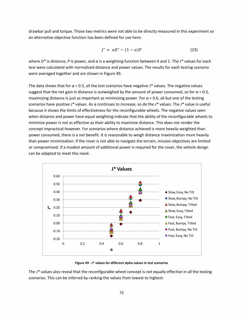
75

drawbar pull and torque. Those two metrics were not able to be directly measured in this experiment so

an alternative objective function has been defined for use here:

(23)

where D* is distance, P is power, and α is a weighting function between 0 and 1. The J* values for each

test were calculated with normalized distance and power values. The results for each testing scenario

were averaged together and are shown in Figure 49.

The data shows that for α = 0.5, all the test scenarios have negative J* values. The negative values

suggest that the net gain in distance is outweighed by the amount of power consumed, so for α = 0.5,

maximizing distance is just as important as minimizing power. For α = 0.6, all but one of the testing

scenarios have positive J* values. As α continues to increase, so do the J* values. The J* value is useful

because it shows the limits of effectiveness for the reconfigurable wheels. The negative values seen

when distance and power have equal weighting indicate that the ability of the reconfigurable wheels to

minimize power is not as effective as their ability to maximize distance. This does not render the

concept impractical however. For scenarios where distance achieved is more heavily weighted than

power consumed, there is a net benefit. It is reasonable to weigh distance maximization more heavily

than power minimization. If the rover is not able to navigate the terrain, mission objectives are limited

or compromised. If a modest amount of additional power is required for the rover, the vehicle design

can be adapted to meet this need.

Figure 49 - J* values for different alpha values in test scenarios

The J* values also reveal that the reconfigurable wheel concept is not equally effective in all the testing

scenarios. This can be inferred by ranking the values from lowest to highest:

-0.20

-0.10

0.00

0.10

0.20

0.30

0.40

0.50

0.60

0 0.2 0.4 0.6 0.8 1

J*

α

J* Values

Slow, Easy, No Tilt

Slow, Bumpy, No Tilt

Slow, Bumpy, Tilted

Slow, Easy, Tilted

Fast, Easy, Tilted

Fast, Bumpy, Tilted

Fast, Bumpy, No Tilt

Fast, Easy, No Tilt

76

1) slow, easy, no tilt

2) slow, easy, tilted

3) slow, bumpy, tilted

4) fast, easy, tilted

5) fast, easy, no tilt

6) slow, bumpy, no tilt

7) fast, bumpy, no tilt

8) fast, bumpy, tilted

When comparing the net effectiveness of maximizing distance and minimizing power, inclination seems

to have had the smallest effect, and ease of terrain the largest. Easy terrains had lower values while

bumpy terrains had higher values. It seems counterintuitive that the more difficult terrain yielded higher

objective function values, but a plausible explanation for this is that the effectiveness of the

reconfigurable wheels is more pronounced in challenging terrain environments than easy terrain

environments. That idea suggests that the additional power required for larger wheels in the more

difficult terrain is worth the extra cost.

Another way to assess the efficiency of the reconfigurable wheel concept is to look at the ratio of

distance to power. Figure 50 shows the total distance divided by the total power consumed for each test

scenario. The higher this ratio, the higher the net return based upon the net cost. Again, there seems to

be a natural breakpoint in concept efficiency based upon terrain type. All of the bumpy terrain scenarios

had lower readings than the easy terrain scenarios. The bumpy terrain scenarios were filtered secondly

by speed and the easy terrain scenarios by inclination.

Figure 50 - Efficiency calculations for all testing scenarios

0.29

0.200.19

0.26 0.26

0.220.23

0.27

0.00

0.05

0.10

0.15

0.20

0.25

0.30

0.35

Test Scenario

Tota

l Dis

tan

ce /

To

tal P

ow

er [

in/W

]

Overall Efficiency

Slow, Easy, No Tilt

Slow, Bumpy, No Tilt

Slow, Bumpy, Tilted

Slow, Easy, Tilted

Fast, Easy, Tilted

Fast, Bumpy, Tilted

Fast, Bumpy, No Tilt

Fast, Easy, No Tilt

77

A more interesting effectiveness measurement is the relative efficiency. Recall from section 3 that as

part of the initial design analysis, a relative performance efficiency metric was developed (Equation 21).

This metric compares the performance efficiency of a reconfigurable system to the performance

efficiency of a non-reconfigurable system. The performance efficiency of each system was defined as the

ratio of drawbar pull to power (Equation 22). A similar metric is defined here except that the

performance efficiency for each system is defined as the ratio of distance to power. The relative

efficiency is still defined as the ratio of the reconfigurable system efficiency to that of the non-

reconfigurable system; those values are displayed in Figure 51. A relative efficiency value greater than

one indicates that the reconfigurable system is more efficient than the non-reconfigurable system, and

vice versa for a value less than one. There does not appear to be any particular characteristic that

dictated the relative efficiency of the scenarios. The range of values is relatively small and the

differences in the values are gradual. Only three of the test scenarios had a relative efficiency that was

greater than one. Although it would be ideal for relative efficiency values for all scenarios to be greater

than one, these results do not necessarily mean that the concept is ineffective. They corroborate the

results from the J* values in suggesting that when power and distance are weighed equally the net

benefit is not necessarily a positive one. As explained earlier, however, maximizing distance is typically a

higher design objective than minimizing power.

Figure 51 - Relative efficiency values for all test scenarios

As a final assessment, it is interesting to look congruently at the scenario rankings. In Table 8, the

scenarios are listed on the left and relevant values discussed are shown horizontally along the top row.

For each value, the scenarios are ranked from lowest to highest. The rankings are color coded as a visual

aid. It is interesting to see the patterns that do exist and the patterns that do not exist. The scenarios

that had the largest distances did not necessarily also consume the most power. The overall efficiency

ranking closely followed the increase in distance ranking while the relative efficiency ranking more

1.09

0.93 0.940.87

0.80

0.97

1.11 1.10

0.00

0.20

0.40

0.60

0.80

1.00

1.20

1.40

Test Scenario

Rco

nfi

g e

ffic

ien

cy/N

on

-re

con

fig

eff

icie

ncy

Relative Efficiency

Slow, Easy, No Tilt

Slow, Bumpy, No Tilt

Slow, Bumpy, Tilted

Slow, Easy, Tilted

Fast, Easy, Tilted

Fast, Bumpy, Tilted

Fast, Bumpy, No Tilt

Fast, Easy, No Tilt

78

closely matched the percentage increase in distance ranking. The objective function ranking does not

closely coincide with any of the other value rankings. In summary, the data show several trends that can

be explained using terramechanic models, however it is also clear that there is limited understanding in

those models such that they cannot adequately explain all the behaviors exhibited in the data.

Table 8 - Scenario Rankings for All Values

6.4 Error Analysis It is important to identify potential sources of error or explanations for inconsistencies in the data for

this project. One of the main sources of inconsistency was the terrain. Each time the rover would travel

through the popcorn, it would disrupt the surface. Effort was made to return the surface to its original

state after each test, but despite this effort the terrain conditions were not exactly the same for each

test. This undoubtedly caused inconsistencies in the data; however, any rover on the Martian or lunar

surface will certainly experience a wide range of surface conditions even if the soil type isn’t changing,

so the variability in testing conditions may have helped to produce more realistic results.

Another source of error was in the reconfiguration process. Each test began with the wheel in the

smallest width configuration and then eventually the wheels reconfigured to the largest width

configuration. The reconfiguration from small width to large width was controlled by microcontrollers,

but at the end of every test the reconfiguration from large width back to small width was done by hand.

This could have also been done with the microcontroller, but manually reconfiguring the wheels rather

than autonomously reconfiguring them saved time. The wheels had approximately the same starting

position each time, but there was undoubtedly some variation in the starting positions between wheels

and between tests.

Perhaps the largest source of error was in measuring the electrical current in each test. This was done by

connecting a multimeter in series with the electrical circuit used to power the drive motors. During each

test, the current was measured by visually observing the readout on the multimeter. The current usage

was not constant so the first measurement was typically the one that was recorded. A more accurate

way to record current would have been to use a current probe that could record the current

ScenarioTotal

Distance

Increase

in

Distance

% Increase

in

Distance

Total

Power

Increase

in Power

% Increase

in PowerJ*

Overall

Efficiency

Relative

Efficiency

slow, bumpy, tilted 1 1 4 4 8 8 3 1 4

slow, bumpy, no tilt 2 2 3 3 6 7 6 2 3

fast, bumpy, tilted 3 5 5 8 7 6 8 3 5

fast, bumpy, no tilt 4 6 7 5 4 4 7 4 8

slow, easy, ti lted 5 3 2 1 3 3 2 6 2

slow, easy, no tilt 6 7 6 2 1 1 1 8 6

fast, easy, ti lted 7 4 1 7 2 2 4 5 1

fast, easy, no tilt 8 8 8 6 5 5 5 7 7

79

consumption for the entire length of the test and then compute the average value. Unfortunately, a

current probe was not available for use in the experiment so the multimeter was used instead.

For most of the testing scenarios, five tests were conducted. Analyzing the amount of error with a

sample size of only five tests may be unreliable. Therefore, in an effort to quantify the amount of error

inherent in the testing process, a set of 25 tests was conducted for the fast, easy, no tilt testing scenario.

Statistical analysis for this larger sample set was completed, including calculating 90 percent confidence

intervals. The results of this analysis are shown in Table 9 below.

Table 9 - Statistical Values for Set of 25 Samples

Variable Name Mean Standard Deviation

Min Value Max Value 90% Confidence

Interval

Reconfigurable (i.e. Total) Distance [in.]

26.84 5.41 18.00 38.00 +/- 1.85

Increase in Distance [in.] 14.56 4.74 6.00 26.00 +/- 1.62

% Increase in Distance 132.37% 63.57% 46.51% 305.88% +/- 21.71%

Reconfigurable (i.e. Total) Power [W]

99.53 6.31 87.19 116.50 +/- 2.16

Increase in Power [W] 5.57 7.25 -7.63 20.95 +/- 2.48

% Increase in Power 13.27% 17.95% -14.00% 63.26% +/- 6.13%

J* (α = 0.5) -0.07 0.08 -0.23 0.10 +/- 0.027

J* (α = 0.6) 0.08 0.09 -0.09 0.28 +/- 0.031

J* (α = 0.7) 0.24 0.10 0.05 0.46 +/- 0.035

J* (α = 0.8) 0.39 0.12 0.19 0.64 +/- 0.039

Overall Efficiency 0.27 0.06 0.16 0.41 +/- 0.020

Relative Efficiency 1.10 0.33 0.63 1.92 +/- 0.11

Most of the values are nominal, however, several important observations can be made from this table.

The percentage increase in distance has a very large confidence interval. As mentioned earlier in the

discussion, the values for the percentage increase in distance for all the testing scenarios appeared

more random and had a much larger range than other values. The error analysis presented here concurs

with the value comparison between the scenarios that suggested that there is naturally a large amount

of variability within distance and drawbar pull data.

The power increase data is also interesting because its standard deviation is larger than its mean value.

This is because in some of the tests, there was actually a decrease in power consumption between the

reconfigurable and non-reconfigurable systems. It is uncertain whether the decrease in power between

systems can be attributed to unusually large power readings for the non-reconfigurable system or

unusually small power readings for the reconfigurable system. This uncertainty may be an outcome of

the inaccuracies in the current measurements, however. More experimentation is necessary to know for

certain the explanation for this drop in power.

Another important value to note is the confidence interval for the relative efficiency. This metric had a

relatively high confidence interval of +/- 0.11. The relative efficiency value must be greater than one in

80

order to claim that the reconfigurable system is more efficient than the non-reconfigurable system. Only

three of the scenarios had relative efficiencies that were greater than one, however of these three

values the highest was 1.11, so the claim that in these three scenarios the reconfigurable system was

more efficient than the non-reconfigurable system is thus questionable within the 90 percent

confidence interval. Alternatively, many of the scenarios whose relative efficiencies were less than one

actually had values within 0.11 of 1.0. Therefore, it is also plausible that in some of these scenarios,

performing additional testing would yield greater efficiencies for the reconfigurable system than the

non-reconfigurable system. Either way, the data suggests that it is difficult to claim that the

reconfigurable system is substantially more efficient than the non-reconfigurable system, or vice versa.

None of the other error analysis results conflict with claims made from the data analysis discussion in

the previous section. Scatter plots of all the data and tables of relevant statistical values for the other

testing scenarios can be found in the appendix. Comparison of these statistical values between scenarios

will not be discussed here because none of the findings are particularly relevant or interesting.

6.5 Summary of Results The major findings from the data can be summarized as follows:

In all the test scenarios, the rover was able to autonomously reconfigure its wheels and achieve

additional distance. However, the data indicates that the terrain and surface conditions had a

major impact on the additional distance that the rover could achieve when using the

reconfigurable wheels.

As expected, results showed an increase in power when using the reconfigurable wheels. Power

consumption seemed to be more sensitive to localized terrain challenges than global terrain

challenges.

When maximizing vehicle traction is more heavily weighed than minimizing power consumption,

the use of reconfigurable wheels yields a net gain in performance.

Error analysis of the results revealed no major concerns that compromise the observations and

claims made here based on the collected data.

81

7.0 Summary and Conclusions

7.1 Conclusion All objectives of this project were successfully met. New design concepts for reconfigurable wheels were

explored; four working prototypes of the best design were built and integrated onto a rover platform;

the rover’s ability to autonomously reconfigure its wheels was successfully demonstrated; and the data

collected from testing corroborates previous results and shows that the use of reconfigurable wheels

enhances rover mobility in challenging terrain.

Any rover engineer would agree that designing, developing, building, testing, launching, and operating a

real planetary rover takes enormous effort and tremendous teamwork. There is still a lot of design,

development, and testing that must be completed before reconfigurable wheels can actually be

implemented on real rovers, but the results of this project have hopefully brought that goal closer.

Previous work from de Weck’s research group showed that the concept of a reconfigurable wheel was

beneficial from a theoretical standpoint, and results from the 62x project showed that in multiple soil

types the amount of drawbar pull a wheel can produce was increased by changing the wheel size. As

part of this project, two different reconfigurable wheel designs for various sized rovers have been

developed. Although only one of the designs was built and tested, its successful integration with an

entire rover platform shows that the reconfigurable wheel concept is practical from a systems

perspective. The wheel is autonomously controlled and capable of supporting the weight of an entire

rover, thus demonstrating that it can effectively function on the surface of another planet regardless of

the absence of human assistance and control.

7.2 Future Work Many important lessons learned throughout the course of this project can help shape plans for future

work. There were several structural problems when the wheel was integrated to the rover platform that

required quick fixes and re-designs. Since every rover design is different, it is not possible to create a

universal design to integrate the wheels onto any rover. However, this project has demonstrated that

there are changes that can make the integration easier. The initial structural problems arose because

the wheel axle was too small compared to the wheel. Due to various constraints, using different drive

motors was not an option for this project; it is recommended that larger wheel axles and motor shafts

be used.

The second structural problem was a result of misalignments between the hubcaps. In the current

designs, the hubcaps are only connected via the linear actuator. In future designs, it is recommended

that either a stronger linear actuator be used or that additional supporting structures that will maintain

hubcap alignment be included.

The final recommendation regarding the wheel design is that there should be fewer gaps in the tire’s

surface area. In the 62x project the tire strips overlapped each other and caused friction problems when

the tire strips tried to slide across each other. Consequently, the current wheel design was changed to

have rectangular tire strips. This means that when the wheel is in its smallest width configuration there

are often large gaps in between the strips. This has not caused any specific problems per se; however, a

82

greater surface area will most likely contribute to better wheel traction. Therefore, it is recommended

that different shapes for the tire strips be experimented with in future designs.

The biggest opportunity for future research for this project lies in the area of autonomy and control.

Multiple studies have now gathered data to support the concept of a reconfigurable wheel, but whether

or not the concept can meet its full potential is dependent on the ability to properly control it. The

control algorithm used in this project was very simplistic, since the testing procedure was designed to

ensure that the wheel would experience slippage and need to change to a wider configuration. The

optimal controller should be capable of changing the wheel to a wide configuration when the rover is

losing traction, but also capable of changing the wheel to a narrow configuration when the rover has

sufficient traction. Additional work should include configuration testing from large to small width.

Additionally, the controller for this project used only two different wheel configurations—smallest width

or largest width. Previous data suggests that in some soils intermediate configurations would be best, so

an optimal controller would need to be capable of configuring to intermediate sizes as well. If new

control algorithms are developed and implemented, the same series of tests conducted in this project

could be carried out for the new controllers. The results could then be compared to see which algorithm

was most effective. Another possibility would be to conduct the same series of tests outlined in the test

matrix in Figure 42, but have a medium width state that the wheel can configure to before changing to

the widest width state (Figure 52).

Figure 52 - Potential test diagram for future testing

Several other testing options can also be recommended. The testing for this project was done in

popcorn seeds to avoid potential problems with sand and dust. If the problems with the wheel design

can be addressed so that dust is less hazardous, then testing in sand would be advisable since sand is the

most problematic soil type on the Martian surface. More variety can also be added to the testing

environment. For example, the inclination of the testbed can be raised, and the tests can be conducted

83

at additional speed settings. New variables—moisture content, for example—can also be introduced to

the test matrix. New tests that experiment with movement strategies can also be tried. For example, as

discussed earlier, the rover often had more difficulty restarting after it stopped in the soil to reconfigure

the wheels due to additional sinkage. Therefore it could be more effective to have the rover back-up a

short distance before moving forward again to increase vehicle momentum. Overall, the data collected

from this project is useful, but there are still many more opportunities for future testing and design

improvements to enhance the concept.

7.3 Closing Statement Designing wheels for Mars rovers has been a great challenge and a thrilling opportunity. The

contributions made from this project are small compared to the vast reservoirs of knowledge required

to successfully send a rover to another planetary surface. Although these contributions are small, it is

hopeful that they will work to expand man’s reach to understand other worlds and aid in the quest to

explore the beauties and mysteries of space and the heavens.

Figure 53 - Image Collage: MER on the left, reconfigurable wheel rover on the right, Apollo 1 Hills in the background (MER and Apollo 1 Hills pictures courtesy of NASA)

84

8.0 References *1+ “NASA’s Opportunity Rover Rolls Free on Mars,”

http://marsrovers.nasa.gov/newsroom/pressreleases/20050606a.html (Accessed January 15, 2011).

*2+ M. Wall, “Spirit Rover Remains Silent as Mars Mission Begins 8th Year,”

http://www.space.com/10425-spirit-rover-remains-silent-mars-mission-begins-8th-year.html (Accessed

June 3, 2011).

[3] “NASA’s Spirit Rover Completes Mission on Mars,”

http://www.nasa.gov/mission_pages/mer/news/mer20110525.html (Accessed June 3, 2011).

[4] A. Young, Lunar and Planetary Rovers: The Wheels of Apollo and the Quest for Mars. Praxis Publishing

Ltd., 2007.

[5] A. Ball, J. R. C. Garry, R. D. Lorenz, and V. V. Kerzhanovich, Planetary Landers and Entry Probes.

Cambridge University Press, 2007.

*6+ “Durable NASA Rover Beginning Ninth Year of Mars Work,”

http://www.nasa.gov/mission_pages/mer/news/mer20120124.html (Accessed January 25, 2012).

[7] M. G. Bekker, Introduction to Terrain-Vehicle Systems. University of Michigan Press, 1969.

[8] M. G. Bekker, Theory of Land Locomotion. University of Michigan Press, 1956.

[9] J.Y. Wong, Theory of Ground Vehicles, 4th edition. John Wiley & Sons, 2008.

[10] J.Y. Wong, Terramechanics and Off-Road Vehicle Engineering: Terrain Behaviour, Off-Road Vehicle

Performance and Design, 2nd edition. Elsevier Ltd., 2010.

[11+ J.R. Matijevic et. al., “Characterization of Martian Surface Deposits by the Mars Pathfinder Rover,

Sojourner,” Science, Vol. 278, pp. 1765-1768, 1997.

[12] A. Siddiqi, O.L. de Weck, and K. Iagnemma, “Reconfigurability in Planetary Surface Vehicles:

Modelling Approaches and Test Study.” Journal of the British Interplanetary Society (JBIS), Vol. 59, pp.

450-460, 2006.

[13+ B. Baker and N. Steber, “Reconfigurable Wheels for Planetary Surface Rovers.” 16.622 Final Report,

Department of Aeronautics and Astronautics, Massachusetts Institute of Technology, 2008.

[14] S. H. Crandall, N. C. Dahl, and T.J. Lardner, An Introduction to the Mechanics of Solids: 2nd Edition

with SI Units. McGraw-Hill, 1999.

85

[15] R. Huston and H. Josephs, Practical Stress Analysis in Engineering Design: 3rd Edition. CRC Press,

2009.

[16+ A. Siddiqi, O. de Weck, and J. Hoffman, “Sustainability in System Architectures Through

Reconfigurability: A Case Study of Planetary Surface Vehicles.” International Astronautical Federation –

56th International Astronautical Congress Vol. 8, pp. 5550-5562, 2005.

[17+ A. Siddiqi and O. de Weck, “Reconfigurability in planetary surface vehicles.” Acta Astronautica Vol.

64, pp. 589-601, 2009.

[18+ K. Iagnemma, H. Shilby and S. Dubowsky, “Online Terrain Parameter Estimation for Wheeled Mobile

Robots with Applications to Planetary Rovers.” IEEE Transactions on Robotics Vol. 20, pp. 921-927,

2004.

[19] J.D. Terry and M.A. Minor, “Traction Estimation and Control for Mobile Robots using the Wheel Slip

Velocity.” Proceedings of the IEEE/RSJ International Conference on Intelligent Robots and Systems, Nice,

France, September 2008.

86

9.0 Appendix

Influence Diagram Several iterations of the influence diagram were created. For one of the final versions, the names of

relevant properties were replaced by the actual variables. That variable diagram and its accompanying

influence diagram can be seen here.

Figure 54 - Earlier version of the influence diagram

87

Figure 55 - Influence diagram with variables

88

Incidence Matrix

In conjunction with the influence diagram, an incidence matrix was also created to show the

relationships between variables. The variables listed horizontally on the top are inputs and the variables

listed vertically on the side are outputs. An ‘x’ indicates that an output variable is influenced by an input

variable. A black ‘x’ indicates a direct relationship and a red ‘x’ indicates an indirect relationship.

Figure 56 - Incidence matrix showing dependencies between relevant variables

X X X X X X X X X X X X X

X X X X X X X

X X X X X X X X

X X

X X X

X X X X X

X X X X X

X

X X X X X X X X X X X X X

X X X X X

X X X X X X X X X

X X X X X X X X X X X X X X X X X X

X X X X X X X X X X X X X X X X

X X X X X

X X X X X

X X X X X X X X X X X X X X X X X X X X X X X

Co

nsu

med

po

wer

Compaction

Resistance

Performance

Fatigue/Wear

Deformation

Power to

reconfigure

Tire Strength

Actuator Type

Tire material

Surface Contact

Area (A)

Slippage (i)

Rover Speed

sin

kage

(z)

Power to drive

DP

Tractive Force (F)

Bull-dozing

Resistance

Sinkage (z)

wh

eel l

oad

(W

)

terr

ain

rove

r lif

etim

e

effe

ctiv

enes

s o

f

con

tro

ller

DP

trac

tive

fo

rce

(F)

soil

resi

stan

ces

rove

r sp

eed

slip

pag

e (i

)

cost

wh

eel w

idth

(b

)

wh

eel d

iam

eter

(D

)

surf

ace

con

tact

area

(A

)

po

wer

ava

ilab

le

po

wer

req

uir

ed

per

act

uat

or

actu

ato

r ty

pe

tire

mat

eria

l

tire

des

ign

(i.e

.

size

/sh

ape)

# o

f ac

tuat

ors

tire

str

engt

h

soil

pro

per

ties

mo

tor

effi

cien

cy

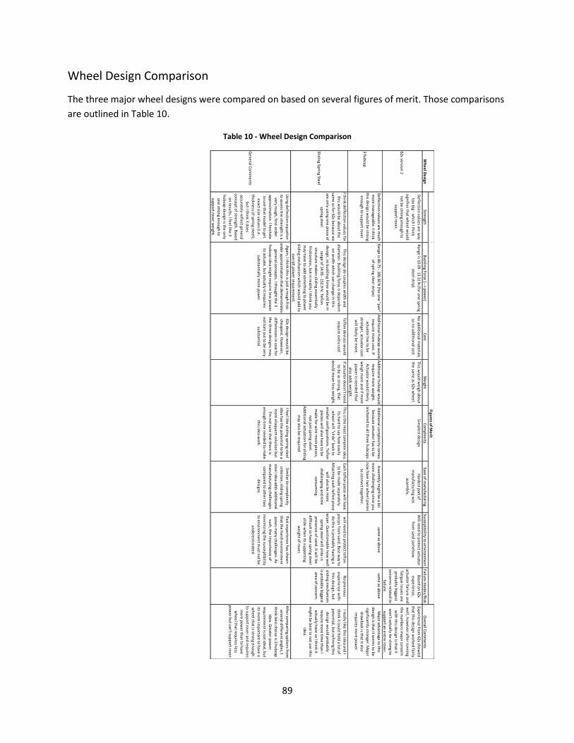
89

Wheel Design Comparison

The three major wheel designs were compared on based on several figures of merit. Those comparisons

are outlined in Table 10.

Table 10 - Wheel Design Comparison

Stren

gthB

ucklin

g Force

(--> po

we

r)C

ost

We

ight

Co

mp

lexity

Ease o

f man

ufactu

ring

Susce

ptib

ility to e

nviro

nm

en

tFailu

re m

od

es/R

isk

62x versio

n 2

De

flectio

n valu

es are

way

too

big - w

hich

I thin

k

signifie

s that w

he

el w

ou

ld

no

t be

stron

g en

ou

gh to

sup

po

rt rove

r.

Ran

ge is 10.09 - 13.31 N

(for o

ne

sprin

g

stee

l strip)

No

add

ition

al mate

rials

so n

o ad

ditio

nal co

st

This w

ou

ld w

eigh

abo

ut

the

same

as 62x wh

ee

l.

Simp

lest d

esign

Hard

est p

art of

man

ufactu

ring w

as

assem

bly.

Will n

ee

d to

pro

tect actu

ator

from

sand

som

eh

ow

.

Base

d o

n 62x

exp

erie

nce

,

actuato

r failure

and

fatigue

issue

s are

pro

bab

ly bigge

st

con

cern

s relate

d to

failure

.

Expe

rien

ce fro

m 62x sh

ow

ed

that th

is de

sign w

orke

d fairly

we

ll, ho

we

ver afte

r run

nin

g

the

nu

mb

ers m

ajor co

nce

rn

with

this d

esign

is that it

wo

n't actu

ally be

stron

g to

sup

po

rt an e

ntire

rove

r.

3 hu

bcap

De

flectio

n valu

es are

mu

ch

mo

re m

anage

able

. I thin

k

this d

esign

wo

uld

be

stron

g

en

ou

gh to

sup

po

rt rove

r

Ran

ge is 80.75 - 106.50 N

(for o

ne

"pair"

of sp

ring ste

el strip

s)

Ad

ditio

nal h

ub

cap w

ou

ld

req

uire

mo

re co

st. If

actuato

r has to

be

stron

ger, actu

ator co

st

will like

ly be

mo

re.

Ad

ditio

nal h

ub

cap w

ou

ld

req

uire

mo

re w

eigh

t.

Actu

ator w

ou

ld like

ly

we

igh m

ore

and

if mo

re

po

we

r is ne

ed

ed

that

also ad

ds w

eigh

t.

Ad

ditio

nal co

mp

lexity co

me

s

be

cause

actuato

r has to

be

anch

ore

d to

all thre

e h

ub

caps.

Asse

mb

ly migh

t be

a bit

mo

re ch

allen

ging sin

ce yo

u

no

w h

ave tw

o w

he

el p

iece

s

to co

nn

ect to

geth

er.

same

as abo

vesam

e as ab

ove

Majo

r advan

tage to

this

de

sign is th

at it see

ms to

be

signfican

tly stron

ger. M

ajor

draw

back is th

at it also

req

uire

s mo

re p

ow

er.

Slidin

g Sprin

g Stee

l

I thin

k de

flectio

n valu

es fo

r

this w

ou

ld b

e ab

ou

t the

same

as for 62x b

ecau

se w

e

are o

nly u

sing o

ne

pie

ce o

f

sprin

g stee

l

This d

esign

de

-cou

ple

s wid

th an

d

diam

ete

r. Bu

ckling fo

rce is d

ep

en

de

nt

on

wid

th w

hich

can ch

ange

in th

is

de

sign, so

bu

ckling fo

rce w

ou

ld b

e in

range

of 14.93 - 152.9 N

. Teflo

n

structu

re m

akes slid

ing e

ssen

tially

friction

less, b

ut in

reality I th

ink yo

u

may h

ave to

add

som

eth

ing to

po

we

r

slidin

g me

chan

ism w

hich

wo

uld

add

to

ove

rall po

we

r req

uire

me

nt.

Teflo

n d

evice

s wo

uld

req

uire

extra co

st

If actuato

r do

esn

't ne

ed

to b

e as stro

ng, th

at

wo

uld

me

an le

ss we

ight.

This is th

e m

ost co

mp

lex id

ea.

Its hard

to say h

ow

easily

wh

ee

l will "slid

e" b

ack to

smalle

r con

figuratio

ns. Te

flon

pie

ces w

ill also h

ave to

be

mad

e fo

r wire

me

sh p

iece

s,

no

t just sp

ring ste

el.

Ad

ditio

nal actu

ation

for slid

ing

may also

be

req

uire

d

Each te

flon

pie

ce w

ill have

to b

e m

ade

sep

arately.

Attach

ing e

ach te

flon

pie

ce

will also

be

mo

re

challe

ngin

g and

time

con

sum

ing.

will n

ee

d to

pro

tect te

flon

pie

ces fro

m san

d. B

est w

ay to

do

this is p

rob

ably h

aving a

wip

er. Q

ue

stion

able

ho

w w

ell

sprin

g stee

l will slid

e in

pre

sen

ce o

f sand

. It will b

e

difficu

lt to h

ave sp

ring ste

el

slide

wh

en

its sup

po

rting

we

ight o

f rove

r.

No

pre

viou

s

exp

erie

nce

with

this d

esign

, bu

t

slidin

g me

chan

ism

is pro

bab

ly bigge

st

area o

f con

cern

.

I really like

this id

ea an

d I

thin

k it cou

ld h

old

a lot o

f

po

ten

tial, bu

t refin

ing th

is

de

sign w

ou

ld p

rob

ably

req

uire

mo

re tim

e th

an I

actually h

ave so

I thin

k it

migh

t be

be

st to n

ot u

se th

is

ide

a.

Ge

ne

ral Co

mm

en

ts

Usin

g de

flectio

n e

qu

ation

to asse

ss tire stre

ngth

is a

very ro

ugh

, first-ord

er

app

roxim

ation

. I he

sitate

to u

se th

at mo

de

l to ge

t

exact size

value

s (i.e.

thickn

ess o

f sprin

g stee

l),

bu

t I thin

k it do

es

accurate

ly refle

ct gen

eral

con

cep

t of stre

ngth

. Base

d

on

resu

lts, I fee

l like 3

hu

bcap

de

sign is th

e o

nly

on

e stro

ng e

no

ugh

to

sup

po

rt rove

r we

ight.

Again

, I thin

k this is ju

st a rou

gh first-

ord

er ap

pro

ximatio

n th

at de

mo

nstrate

s

gen

eral co

nce

pts. I th

ou

ght th

e 3

hu

bcap

ide

a migh

t req

uire

less p

ow

er

to actu

ate, b

ut actu

ally it req

uire

s

sub

stantially m

ore

po

we

r.

62x de

sign w

ou

ld b

e

che

ape

st. Ho

we

ver,

diffe

ren

ces in

cost fo

r

the

thre

e d

esign

s may

no

t turn

ou

t to b

e ve

ry

sub

stantial.

I fee

l like slid

ing sp

ring ste

el

ide

a has th

e p

ote

ntial to

be

a

mo

re e

loq

ue

nt so

lutio

n b

ut

I'm n

ot su

re th

at the

re is

en

ou

gh tim

e n

ee

de

d to

make

this id

ea w

ork.

Similar to

com

ple

xity

criterio

n, slid

ing sp

ring

stee

l ide

a add

s add

ition

al

man

ufactu

ring ch

allen

ges

com

pare

d to

oth

er tw

o

de

signs.

Past e

xpe

rien

ce h

as sho

wn

that th

e h

arsh e

nviro

nm

en

t

po

ses m

any ch

allen

ges. A

s

such

, the

imp

ortan

ce o

f

min

imizin

g the

susce

ptib

ility

to e

nviro

nm

en

t mu

st no

t be

un

de

restim

ated

.

Afte

r com

parin

g op

tion

s from

seve

ral diffe

ren

t angle

s, I

thin

k be

st cho

ice is 3 h

ub

cap

ide

a. Gre

ater p

ow

er

req

uire

me

nt is n

ot id

eal, b

ut

its mo

re im

po

rtant to

have

a

wh

ee

l that is stro

ng e

no

ugh

to su

pp

ort ro

ver an

d re

qu

ires

mo

re p

ow

er th

an to

have

wh

ee

l that re

qu

ires le

ss

po

we

r bu

t can't su

pp

ort ro

ver.

Wh

ee

l De

signO

verall C

om

me

nts

Figure

s of M

erit

90

Material Properties for Composite Tire Strips

Table 11 - Material properties for tire strips

Material Properties of Spring Steel/Wire Mesh Combo

Property Value Units

Elastic Modulus 4.24*10^10 Pa

Poisson's ratio 0.287 NA

Density 0.283 lbs/in^3

Tensile Strength 142 ksi

Yield Strength 80 ksi

Thermal Expansion Coefficient

8.1*10^-6 /° F

Thermal Conductivity 27 Btu/sq. ft./ft./hr./° F

91

Deflection Results from Beam Modeling

Figure 57 - Simple beam theory deflection results for 3hubcap wheel design. The different colors represent different tire strip lengths. The x-axis is the distance along the length of the tire strip and the y-axis is the amount of deflection.

Figure 58 - Simple beam theory deflection results for 62x_ver2 wheel design. The different colors represent different tire strip lengths. The x-axis is the distance along the length of the tire strip and the y-axis is the amount of deflection.

92

Figure 59 - Thin curved beam theory deflection results for the 3hubcap wheel design. The different colors represent different tire strip lengths. The x-axis is the distance along the length of the tire strip and the y-axis is the amount of deflection.

Figure 60 - Thin curved beam theory results for the 62x_ver2 wheel design. The different colors represent different tire strip lengths. The x-axis is the distance along the length of the tire strip and the y-axis is the amount of deflection.

93

Manufacturability Assessment

After the wheel design selection, the manufacturability of the reconfigurable wheel was evaluated

based on whether or not parts were commercially available (COTS), material costs, fabrication needs,

assembly needs, and the availability of resources to meet the assembly and fabrication needs.

Table 12 – Manufacturability assessment for the 62x_ver2 and 3hubcap wheel designs

Parts List COTS?Material

CostFabrication Needs Assembly Needs Resource Availability

Hubcaps No 37.5

Pieces have to be cut using

water jet, drilled for screws

and actuator using mill,

tapped by hand

Aero/Astro Machine Shop Capability

Wire Mesh No 105 Pieces have to be cut by handspring steel and wire mesh has

to be "sewn" by handAero/Astro Machine Shop Capability

Spring Steel No 30Pieces have to be cut using

water jet

spring steel and wire mesh

pieces have to be secured to

hubcaps

Aero/Astro Machine Shop Capability

Actuator Yes ?Set screws for linear actuator

need to be made

Actuator has to be mounted to

hubcapsAero/Astro Machine Shop Capability

Retaining Ring/Flange No 37.5

Pieces have to be cut using

water jet, drilled using mill,

tapped by hand

Aero/Astro Machine Shop Capability

Screws Yes 5

Microcontroller Yes 250Programming for

microcontroller, all of the

Laptop Computer and OpenSource

Software

Encoders Yes 40 Puchase from VEX Robotics

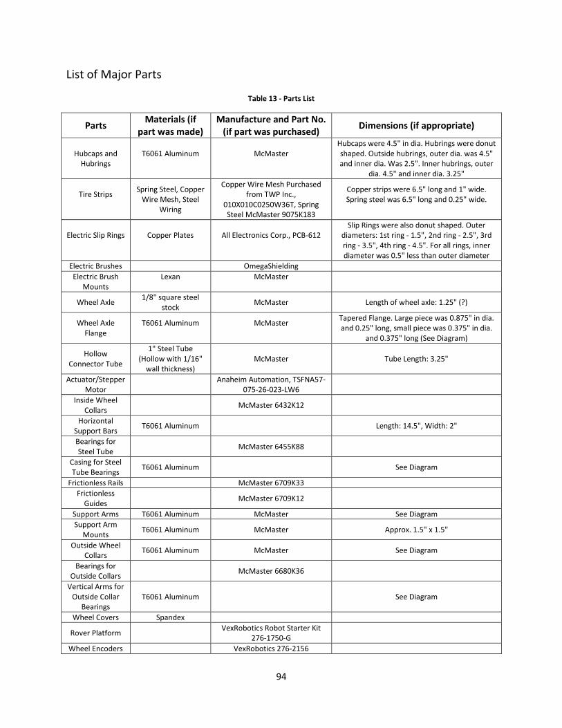
94

List of Major Parts

Table 13 - Parts List

Parts Materials (if

part was made) Manufacture and Part No.

(if part was purchased) Dimensions (if appropriate)

Hubcaps and Hubrings

T6061 Aluminum

McMaster

Hubcaps were 4.5" in dia. Hubrings were donut shaped. Outside hubrings, outer dia. was 4.5" and inner dia. Was 2.5". Inner hubrings, outer

dia. 4.5" and inner dia. 3.25"

Tire Strips

Spring Steel, Copper Wire Mesh, Steel

Wiring

Copper Wire Mesh Purchased from TWP Inc.,

010X010C0250W36T, Spring Steel McMaster 9075K183

Copper strips were 6.5" long and 1" wide. Spring steel was 6.5" long and 0.25" wide.

Electric Slip Rings

Copper Plates

All Electronics Corp., PCB-612

Slip Rings were also donut shaped. Outer diameters: 1st ring - 1.5", 2nd ring - 2.5", 3rd ring - 3.5", 4th ring - 4.5". For all rings, inner diameter was 0.5" less than outer diameter

Electric Brushes OmegaShielding

Electric Brush Mounts

Lexan

McMaster

Wheel Axle 1/8" square steel

stock McMaster Length of wheel axle: 1.25" (?)

Wheel Axle Flange

T6061 Aluminum

McMaster

Tapered Flange. Large piece was 0.875" in dia. and 0.25" long, small piece was 0.375" in dia.

and 0.375" long (See Diagram)

Hollow Connector Tube

1" Steel Tube (Hollow with 1/16"

wall thickness) McMaster Tube Length: 3.25"

Actuator/Stepper Motor

Anaheim Automation, TSFNA57-

075-26-023-LW6

Inside Wheel Collars

McMaster 6432K12

Horizontal Support Bars

T6061 Aluminum Length: 14.5", Width: 2"

Bearings for Steel Tube

McMaster 6455K88

Casing for Steel Tube Bearings

T6061 Aluminum See Diagram

Frictionless Rails McMaster 6709K33

Frictionless Guides

McMaster 6709K12

Support Arms T6061 Aluminum McMaster See Diagram

Support Arm Mounts

T6061 Aluminum McMaster Approx. 1.5" x 1.5"

Outside Wheel Collars

T6061 Aluminum McMaster See Diagram

Bearings for Outside Collars

McMaster 6680K36

Vertical Arms for Outside Collar

Bearings T6061 Aluminum See Diagram

Wheel Covers Spandex

Rover Platform VexRobotics Robot Starter Kit

276-1750-G

Wheel Encoders VexRobotics 276-2156

95

Arduino Uno Microcontroller

SparkFun DEV-09950

Stepper Motor Drivers

Marlin P. Jones Assoc., 18187MS

LiPo Batteries (for Drivers)

Hobby Lobby International Inc.,

YTB13004

96

Dimensional Drawings for some of the Custom-Made Parts

Figure 61 - Dimensional drawings of inner hubcap and aluminum plug

97

Figure 62 - Dimensional drawing for bearings for hollow steel tube

Figure 63 - Dimensional drawing for support arms

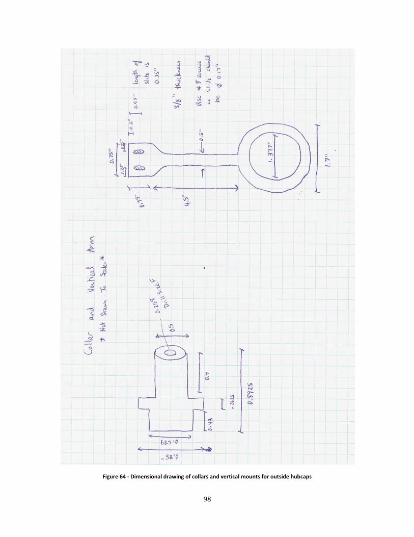
98

Figure 64 - Dimensional drawing of collars and vertical mounts for outside hubcaps

99

Specs for Major Hardware Components

Figure 65 - Specification sheet for linear actuator

100

Figure 66 - Specification sheet for stepper motor driver

101

Stepper Motor Overview

Stepper motors operate differently than regular DC motors. As diagramed in the lower left of Figure 67,

stepper motors are built from two electromagnets (marked as 1 and 2 in the diagram) and a 6-pole

magnetic rotor. As the electromagnets are energized in sequence, the rotor turns. Figure 67 also

includes a timing diagram and phase diagram as visualization tools. The axes in the phase diagram

represent the input signals for each electromagnetic. The timing diagram also show the input signals for

each electromagnet but here they are shown separately as a function of time. As can be seen from

either diagram, four different states are possible (marked as 0, 1, 2, or 3). Both electromagnets can be

high, both can be low, or they can be opposite each other. The frequency of the signal determines the

speed that the motor turns at and the sequence of the signals determines the direction. This type of

design allows for precise positioning without the need for feedback. In order to control the stepper

motors, a direction command and a square pulse wave is sent to the motor driver. The motor driver

then translates those commands into the proper sequence of pulses to move the motor. The motor

driver is analogous to a compiler. The user writes the source code but then the driver translates that

code into the assembly language that the motor needs to run.

Figure 67 - Stepper motor diagrams

102

Electrical System Setup

Figure 68 - All of the connections for the electrical system

103

Test Plan

The testing procedure is outlined below.

1. Make sure all rover electronics are unplugged and turned off

2. Remove voltmeter

3. Manually put wheels in smallest width configuration

4. Replace voltmeter and turn it on

5. Position rover at starting point in trench

6. Connect Cortex microcontroller to laptop using USB to USB cord

7. Mark starting location of rover

8. Run robotC code from laptop

9. While rover is moving forward, observe and record average current reading from voltmeter

10. Once rover stops, measure and record how far rover has traveled

11. Reconfigure wheels to widest width

a. Remove voltmeter

b. Plug in driver batteries

c. Plug in Arduino microcontroller

d. After wheels have reached widest width unplug microcontroller

e. Unplug driver batteries

f. Replace voltmeter

12. Mark location of rover

13. Run robotC code from laptop

14. While rover is moving forward, record average current reading from voltmeter

15. Once rover stops, measure and record how far rover has traveled (measurement taken from

point in step 12)

104

Scatter Plots and Statistical Tables

Scatter plots showing the data for all different test scenarios are shown below. The scatter plots show

the power and distance results for the non-reconfigurable and reconfigurable systems. Tables showing

statistics for other relevant values are also shown for each scenario.

Figure 69 - Power and distance data for slow, easy, no tilt scenario

Table 14 - Statistics for slow, easy, no tilt scenario

Variable Name Mean Standard Deviation

Min Value Max Value

Reconfigurable (i.e. Total) Distance [in.]

26.3 11.76 14 44

Increase in Distance [in.] 13.8 5.97 9 24

% Increase in Distance 121.52% 38.21% 74.29% 180.00%

Reconfigurable (i.e. Total) Power [W]

92.87 6.59 82.87 100.80

Increase in Power [W] 1.14 3.18 -1.08 6.70

% Increase in Power 2.64% 7.44% -2.57% 15.66%

J* (α = 0.5) -0.16 0.15 -0.30 0.04

J* (α = 0.6) -0.01 0.17 -0.18 0.23

J* (α = 0.7) 0.14 0.19 -0.05 0.43

J* (α = 0.8) 0.29 0.22 0.07 0.62

Overall Efficiency 0.29 0.13 0.15 0.48

Relative Efficiency 1.09 0.20 0.88 1.41

0

5

10

15

20

25

30

35

40

0.00 20.00 40.00 60.00 80.00 100.00 120.00 140.00

Dis

tan

ce [i

n.]

Power [W]

Test Scenario: slow, easy, no tilt

Non-reconfigurable Wheels Reconfigurable Wheels

105

Figure 70 - Power and distance data for slow, easy, tilted scenario

Table 15 – Statistics for slow, easy, tilted scenario

Variable Name Mean Standard Deviation

Min Value Max Value

Reconfigurable (i.e. Total) Distance [in.]

23.9 7.16 14 32.5

Increase in Distance [in.] 10.1 4.77 6 15.5

% Increase in Distance 81.33% 42.75% 37.50% 133.33%

Reconfigurable (i.e. Total) Power [W]

91.07 3.35 87.26 96.05

Increase in Power [W] 3.60 2.44 1.58 7.78

% Increase in Power 8.21 5.50 3.63 17.62

J* (α = 0.5) -0.11 0.12 -0.28 0.02

J* (α = 0.6) 0.06 0.14 -0.14 0.22

J* (α = 0.7) 0.23 0.16 0.00 0.41

J* (α = 0.8) 0.40 0.18 0.14 0.61

Overall Efficiency 0.26 0.08 0.15 0.35

Relative Efficiency 0.87 0.19 0.67 1.07

0

5

10

15

20

25

30

35

40

0.00 20.00 40.00 60.00 80.00 100.00 120.00 140.00

Dis

tan

ce [i

n.]

Power [W]

Test Scenario: slow, easy, tilt

Non-reconfigurable Wheels Reconfigurable Wheels

106

Figure 71 - Power and distance data for slow, bumpy, tilted scenario

Table 16 - Statistics for slow, bumpy, tilted scenario

Variable Name Mean Standard Deviation

Min Value Max Value

Reconfigurable (i.e. Total) Distance [in.]

17.9 3.73 14 23

Increase in Distance [in.] 8.4 1.19 7 10

% Increase in Distance 102.01% 49.44% 57.69% 181.82%

Reconfigurable (i.e. Total) Power [W]

94.62 4.79 87.41 100.51

Increase in Power [W] 6.81 6.05 -1.15 15.05

% Increase in Power 16.45% 15.08% -2.44% 36.99%

J* (α = 0.5) -0.08 0.08 -0.16 0.03

J* (α = 0.6) 0.09 0.09 -0.01 0.22

J* (α = 0.7) 0.26 0.11 0.15 0.42

J* (α = 0.8) 0.43 0.13 0.30 0.61

Overall Efficiency 0.19 0.04 0.15 0.24

Relative Efficiency 0.94 0.23 0.67 1.26

0

5

10

15

20

25

30

35

40

0.00 20.00 40.00 60.00 80.00 100.00 120.00 140.00

Dis

tan

ce [i

n.]

Power [W]

Test Scenario: slow, bumpy, tilt

Non-reconfigurable Wheels Reconfigurable Wheels

107

Figure 72 - Power and distance data for slow, bumpy, no tilt scenario

Table 17 - Statistics for slow, bumpy, no tilt scenario

Variable Name Mean Standard Deviation

Min Value Max Value

Reconfigurable (i.e. Total) Distance [in.]

18.8 2.44 16 22.5

Increase in Distance [in.] 9.1 1.19 7.5 10.5

% Increase in Distance 98.28% 26.76% 62.50% 133.33%

Reconfigurable (i.e. Total) Power [W]

93.47 9.73 79.78 104.04

Increase in Power [W] 6.03 5.18 1.15 13.68

% Increase in Power 14.04% 12.08% 2.93% 31.25%

J* (α = 0.5) -0.03 0.07 -0.14 0.05

J* (α = 0.6) 0.14 0.08 0.03 0.24

J* (α = 0.7) 0.32 0.08 0.20 0.43

J* (α = 0.8) 0.49 0.09 0.37 0.62

Overall Efficiency 0.20 0.03 0.15 0.24

Relative Efficiency 0.93 0.17 0.70 1.15

0

5

10

15

20

25

30

35

40

0.00 20.00 40.00 60.00 80.00 100.00 120.00 140.00

Dis

tan

ce [i

n.]

Power [W]

Test Scenario: slow, bumpy, no tilt

Non-reconfigurable Wheels Reconfigurable Wheels

108

Figure 73 - Power and distance data for fast, easy, no tilt scenario

*Note: In the fast, easy, no tilt scenario 25 tests were completed so that an error analysis could be

completed.

Table 18 - Statistics for fast, easy, no tilt scenario

Variable Name Mean Standard Deviation

Min Value Max Value 90% Confidence

Interval

Reconfigurable (i.e. Total) Distance [in.]

26.84 5.41 18.00 38.00 +/- 1.85

Increase in Distance [in.] 14.56 4.74 6.00 26.00 +/- 1.62

% Increase in Distance 132.37% 63.57% 46.51% 305.88% +/- 21.71%

Reconfigurable (i.e. Total) Power [W]

99.53 6.31 87.19 116.50 +/- 2.16

Increase in Power [W] 5.57 7.25 -7.63 20.95 +/- 2.48

% Increase in Power 13.27% 17.95% -14.00% 63.26% +/- 6.13%

J* (α = 0.5) -0.07 0.08 -0.23 0.10 +/- 0.027

J* (α = 0.6) 0.08 0.09 -0.09 0.28 +/- 0.031

J* (α = 0.7) 0.24 0.10 0.05 0.46 +/- 0.035

J* (α = 0.8) 0.39 0.12 0.19 0.64 +/- 0.039

Overall Efficiency 0.27 0.06 0.16 0.41 +/- 0.020

Relative Efficiency 1.10 0.33 0.63 1.92 +/- 0.11

0

5

10

15

20

25

30

35

40

0.00 20.00 40.00 60.00 80.00 100.00 120.00 140.00

Dis

tan

ce [i

n.]

Power [W]

Test Scenario: fast, easy, no tilt

Non-reconfigurable Wheels Reconfigurable Wheels

109

Figure 74 - Power and distance data for fast, easy, tilted scenario

Table 19 - Statistics for fast, easy, tilted scenario

Variable Name Mean Standard Deviation

Min Value Max Value

Reconfigurable (i.e. Total) Distance [in.]

26.7 6.32 18.00 35.00

Increase in Distance [in.] 10.5 3.08 7.00 15.00

% Increase in Distance 64.30 7.94 54.29 75.00

Reconfigurable (i.e. Total) Power [W]

102.66 5.77 97.20 112.03

Increase in Power [W] 2.43 7.00 -4.32 13.54

% Increase in Power 5.81 15.52 -7.98 31.18

J* (α = 0.5) -0.08 0.07 -0.19 0.00

J* (α = 0.6) 0.09 0.09 -0.05 0.20

J* (α = 0.7) 0.26 0.11 0.09 0.40

J* (α = 0.8) 0.43 0.14 0.23 0.60

Overall Efficiency 0.26 0.05 0.18 0.31

Relative Efficiency 0.80 0.07 0.71 0.88

0

5

10

15

20

25

30

35

40

0.00 20.00 40.00 60.00 80.00 100.00 120.00 140.00

Dis

tan

ce [i

n.]

Power [W]

Test Scenario: fast, easy, tilt

Non-reconfigurable Wheels Reconfigurable Wheels

110

Figure 75 - Power and distance data for fast, bumpy, tilted scenario

Table 20 - Statistics for fast, bumpy, tilted scenario

Variable Name Mean Standard Deviation

Min Value Max Value

Reconfigurable (i.e. Total) Distance [in.]

22.8 2.36 20.5 26

Increase in Distance [in.] 11.4 2.68 9 16

% Increase in Distance 104.96% 37.44% 60.00% 160.00%

Reconfigurable (i.e. Total) Power [W]

104.77 5.49 100.01 114.12

Increase in Power [W] 6.16 6.19 -0.36 14.76

% Increase in Power 13.62% 14.56% -0.69% 34.63%

J* (α = 0.5) -0.02 0.06 -0.11 0.04

J* (α = 0.6) 0.16 0.06 0.07 0.23

J* (α = 0.7) 0.34 0.07 0.25 0.43

J* (α = 0.8) 0.52 0.08 0.43 0.62

Overall Efficiency 0.22 0.03 0.18 0.25

Relative Efficiency 0.97 0.21 0.77 1.30

0

5

10

15

20

25

30

35

40

0.00 20.00 40.00 60.00 80.00 100.00 120.00 140.00

Dis

tan

ce [i

n.]

Power [W]

Test Scenario: fast, bumpy, tilt

Non-reconfigurable Wheels Reconfigurable Wheels

111

Figure 76 - Power and distance data for fast, bumpy, no tilt scenario

Table 21 - Statistics for fast, bumpy, no tilt scenario

Variable Name Mean Standard Deviation

Min Value Max Value

Reconfigurable (i.e. Total) Distance [in.]

22.9 2.58 20 26

Increase in Distance [in.] 12.6 3.31 9 18

% Increase in Distance 130.98% 59.90% 81.82% 225.00%

Reconfigurable (i.e. Total) Power [W]

98.19 6.12 90.29 105.70

Increase in Power [W] 4.94 9.02 -8.93 13.68

% Increase in Power 11.57 18.99 -17.22 29.73

J* (α = 0.5) -0.02 0.07 -0.11 0.05

J* (α = 0.6) 0.16 0.08 0.07 0.24

J* (α = 0.7) 0.34 0.08 0.25 0.43

J* (α = 0.8) 0.52 0.09 0.43 0.62

Overall Efficiency 0.23 0.04 0.19 0.27

Relative Efficiency 1.11 0.38 0.88 1.78

0

5

10

15

20

25

30

35

40

0.00 20.00 40.00 60.00 80.00 100.00 120.00 140.00

Dis

tan

ce [

in.]

Power [W]

Test Scenario: fast, bumpy, no tilt

Non-reconfigurable Wheels Reconfigurable Wheels

112

Figure 77 - Power difference vs. distance difference for all tests

0

5

10

15

20

25

30

-15.00 -10.00 -5.00 0.00 5.00 10.00 15.00 20.00 25.00

Dis

tan

ce D

iffe

ren

ce [

in.]

Power Difference [W]

Power Difference vs. Distance Difference

Slow, Easy, No Tilt

Slow, Bumpy, No Tilt

Slow, Bumpy, Tilted

Slow, Easy, Tilted

Fast, Easy, Tilted

Fast, Bumpy, Tilted

Fast, Bumpy, No Tilt

Fast, Easy, No Tilt