Reconciling multidecadal land-sea global temperaturewith rising CO2

Vaughan PrattStanford University

Vaughan Pratt Stanford University Reconciling multidecadal land-sea global temperature with rising CO2 1 / 29

Goal

Additional insight into

1 Similarity of the 1860-1880 & 1910-1940 rises to 1970-2000.

2 The recent pause (2001-2013).

3 No sign of 3 ◦C per doubling of CO2.

Simple reasoning (no opaque models or sophisticated statistics).

Some applicable audiences:

Average reader of Scientific American, Discover, etc.

Decision makers—because complex reasoning may delay decisions.

Lawyers—because they have to talk to judges and juries.

Vaughan Pratt Stanford University Reconciling multidecadal land-sea global temperature with rising CO2 2 / 29

Part 1: Three Rises

Question: If the first two rises below are natural, why not the third?

Answer: They can be separated using land-sea difference.

.3 LAND + .7 SEA(~ HadCRUT4)

YEAR

LA

ND

+ S

EA

1860 1880 1900 1920 1940 1960 1980 2000

Vaughan Pratt Stanford University Reconciling multidecadal land-sea global temperature with rising CO2 3 / 29

Land-Sea Difference

HadCRUT4 ≈ 0.3 LAND + 0.7 SEA (geographical weighting).

Consider instead LAND − SEA, specifically CRUTEM4 − HadSST3.

.3 LAND + .7 SEA(~ HadCRUT4)

YEAR

LA

ND

+ S

EA

L

AN

D −

SE

A

LAND − SEA

1860 1880 1900 1920 1940 1960 1980 2000

Vaughan Pratt Stanford University Reconciling multidecadal land-sea global temperature with rising CO2 4 / 29

Heat flow direction: The Copper Bar Gedankenexperiment

Heating copper bar at T1 end raises SUM(T1,T2) over time.

T1 T2

TIME

T1 + T2

Vaughan Pratt Stanford University Reconciling multidecadal land-sea global temperature with rising CO2 5 / 29

Heat flow direction: The Copper Bar Gedankenexperiment

SUM is not a diagnostic of direction, witness heating other end.

T1 T2

TIME

T1 + T2

Vaughan Pratt Stanford University Reconciling multidecadal land-sea global temperature with rising CO2 6 / 29

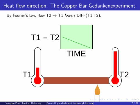
Heat flow direction: The Copper Bar Gedankenexperiment

By Fourier’s law, flow T2 → T1 lowers DIFF(T1,T2).

T1 T2

TIME

T1 - T2

Vaughan Pratt Stanford University Reconciling multidecadal land-sea global temperature with rising CO2 7 / 29

Heat flow direction: The Copper Bar Gedankenexperiment

Dually, flow T1 → T2 raises DIFF. So DIFF indicates direction.

T1 T2

TIME

T1 - T2

Vaughan Pratt Stanford University Reconciling multidecadal land-sea global temperature with rising CO2 8 / 29

Heat flow direction: The Copper Bar Gedankenexperiment

Heating middle (or both ends) balances the flow. DIFF unchanged.

T1 T2

TIME

T1 - T2

Vaughan Pratt Stanford University Reconciling multidecadal land-sea global temperature with rising CO2 9 / 29

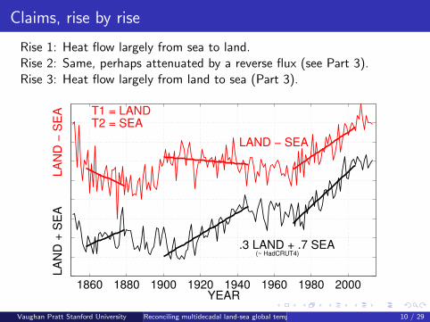
Claims, rise by rise

Rise 1: Heat flow largely from sea to land.Rise 2: Same, perhaps attenuated by a reverse flux (see Part 3).Rise 3: Heat flow largely from land to sea (Part 3).

.3 LAND + .7 SEA(~ HadCRUT4)

YEAR

LA

ND

+ S

EA

L

AN

D −

SE

A

LAND − SEA

T1 = LANDT2 = SEA

1860 1880 1900 1920 1940 1960 1980 2000

Vaughan Pratt Stanford University Reconciling multidecadal land-sea global temperature with rising CO2 10 / 29

Corollaries

1 At successive rises of land-sea sum, the corresponding trends ofland-sea difference shift gradually from strongly negative to stronglypositive.

2 The first two rises of the sum cannot be attributed to atmosphericeffects such as volcanic dimming, natural CO2 fluctuations, etc.

Vaughan Pratt Stanford University Reconciling multidecadal land-sea global temperature with rising CO2 11 / 29

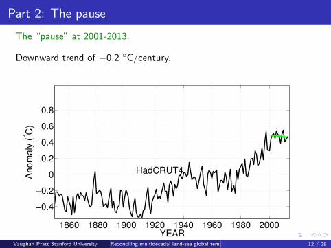
Part 2: The pause

The “pause” at 2001-2013.

Downward trend of −0.2 ◦C/century.

1860 1880 1900 1920 1940 1960 1980 2000

−0.4

−0.2

0

0.2

0.4

0.6

0.8

YEAR

An

om

aly

(°C

)

HadCRUT4

Vaughan Pratt Stanford University Reconciling multidecadal land-sea global temperature with rising CO2 12 / 29

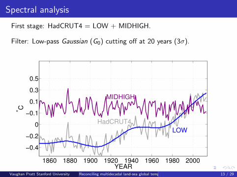
Spectral analysis

First stage: HadCRUT4 = LOW + MIDHIGH.

Filter: Low-pass Gaussian (G0) cutting off at 20 years (3σ).

1860 1880 1900 1920 1940 1960 1980 2000

−0.4

−0.2

0

−0.1

0.1

0.3

0.5

YEAR

°C

HadCRUT4

LOW

MIDHIGH

Vaughan Pratt Stanford University Reconciling multidecadal land-sea global temperature with rising CO2 13 / 29

MID as the 20-year band

Second stage: MIDHIGH = MID + HIGH.

Filter: Band-pass Mexican hat (Ricker, G2) centered on 20 years.

1860 1880 1900 1920 1940 1960 1980 2000

−0.4

−0.2

0

−0.1

0.1

−0.1

0.1

YEAR

°C

HadCRUT4

LOW

MIDHIGH MID

HIGH

HadCRUT4 = HIGH + MID + LOW

Vaughan Pratt Stanford University Reconciling multidecadal land-sea global temperature with rising CO2 14 / 29

Significance of MID

MID is (a) robust and (b) phase-locked with the 20-year solar Hale cycle.

LOW: No pause expected. LOW+MID: Expect a pause.

1860 1880 1900 1920 1940 1960 1980 2000

YEAR

Expectation with LOW

Expectation with LOW+MID

Vaughan Pratt Stanford University Reconciling multidecadal land-sea global temperature with rising CO2 15 / 29

Corollaries

1 When MID is recognized as ongoing, the hiatus is consistent withthe steady recent rise of LOW (whatever its cause).

2 Santer et al’s requirement of 17 years on the minimum periodneeded to detect a trend reliably is too high.

Santer treated MID as part of the unpredictable noise.Treating it as a predictable signalpermits reducing the 17 year figure to the order of a decade.

3 Puzzle: Why no pause in 1980-1990?This needs Part 3.

Vaughan Pratt Stanford University Reconciling multidecadal land-sea global temperature with rising CO2 16 / 29

Part 3. The missing climate sensitivity

Doubling CO2 will eventually raise the temperature 3 ◦C(or whatever the Equilibrium Climate Sensitivity (ECS) actually is).

But what if the CO2 keeps rising?

Transient Climate Response, TCR, is the rise in temperature

during a doubling of CO2

while it is rising at 1%/yr (so 70 years to double).

Can we relate the two?

Proposal: ECS as delayed TCR.

Basis: The ocean as heat sink [Hansen et al 1985]

Quantify this as follows (several steps).

Vaughan Pratt Stanford University Reconciling multidecadal land-sea global temperature with rising CO2 17 / 29

Impact of Human CO2

Cumulative emissions and land use change since 1820.

CDIAC data, in units of GtC.

1820 1840 1860 1880 1900 1920 1940 1960 1980 2000

0

100

200

300

400

500

YEAR

Cu

mu

lative

em

issio

ns (

GtC

)

Fuel+Cement+Land use (CDIAC)

Vaughan Pratt Stanford University Reconciling multidecadal land-sea global temperature with rising CO2 18 / 29

Impact of Human CO2

Rescale GtC to ppmv: divide by 5.148*12/28.97 (matm, AWC , MWair ).

Then add 283 as estimate of pre-1820 atmospheric CO2.

1820 1840 1860 1880 1900 1920 1940 1960 1980 2000

300

350

400

450

500

550

YEAR

Atm

osp

he

ric C

O2

(p

pm

v)

283

Fuel+Cement+Land use (CDIAC)

Vaughan Pratt Stanford University Reconciling multidecadal land-sea global temperature with rising CO2 19 / 29

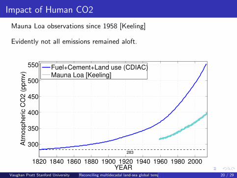
Impact of Human CO2

Mauna Loa observations since 1958 [Keeling]

Evidently not all emissions remained aloft.

1820 1840 1860 1880 1900 1920 1940 1960 1980 2000

300

350

400

450

500

550

YEAR

Atm

osp

he

ric C

O2

(p

pm

v)

283

Fuel+Cement+Land use (CDIAC)Mauna Loa [Keeling]

Vaughan Pratt Stanford University Reconciling multidecadal land-sea global temperature with rising CO2 20 / 29

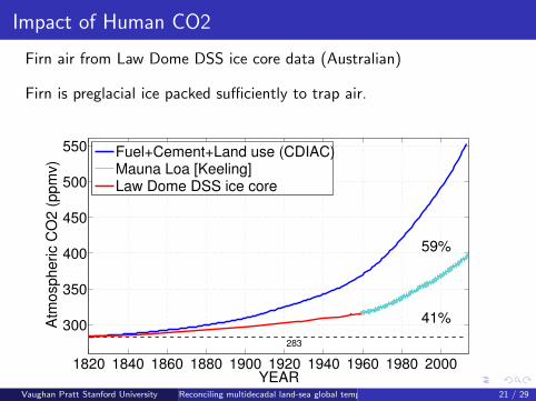
Impact of Human CO2

Firn air from Law Dome DSS ice core data (Australian)

Firn is preglacial ice packed sufficiently to trap air.

1820 1840 1860 1880 1900 1920 1940 1960 1980 2000

300

350

400

450

500

550

YEAR

Atm

osp

he

ric C

O2

(p

pm

v)

283

59%

41%

Fuel+Cement+Land use (CDIAC)Mauna Loa [Keeling]Law Dome DSS ice core

Vaughan Pratt Stanford University Reconciling multidecadal land-sea global temperature with rising CO2 21 / 29

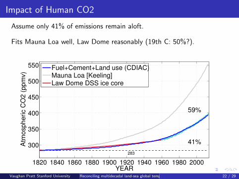
Impact of Human CO2

Assume only 41% of emissions remain aloft.

Fits Mauna Loa well, Law Dome reasonably (19th C: 50%?).

1820 1840 1860 1880 1900 1920 1940 1960 1980 2000

300

350

400

450

500

550

YEAR

Atm

osp

he

ric C

O2

(p

pm

v)

283

59%

41%

Fuel+Cement+Land use (CDIAC)Mauna Loa [Keeling]Law Dome DSS ice core

Vaughan Pratt Stanford University Reconciling multidecadal land-sea global temperature with rising CO2 22 / 29

Impact of Human CO2

Arrhenius Law: LOGCO2 = log2(CO2/280). (Use CDIAC for CO2.)

Expected global warming @ climate sensitivity 1◦C/CO2 doubling.

1820 1840 1860 1880 1900 1920 1940 1960 1980 2000−0.4

−0.3

−0.2

−0.1

0

0.1

0.2

0.3

0.4

0.5

0.6

YEAR

CO

2 F

orc

ing

(°C

)

LOGCO2 = log2(CO2/280)

LOGCO2

Vaughan Pratt Stanford University Reconciling multidecadal land-sea global temperature with rising CO2 23 / 29

Fitting LOGCO2 to LOW

Introduce LOW as below. Coming up: fit LOGCO2 to it...

...in order to analyze LOW = AGW + RESIDUAL.

1820 1840 1860 1880 1900 1920 1940 1960 1980 2000−0.4

−0.3

−0.2

−0.1

0

0.1

0.2

0.3

0.4

0.5

0.6

YEAR

An

om

aly

(°C

)

LOGCO2 = log2(CO2/280)

LOGCO2LOW

Vaughan Pratt Stanford University Reconciling multidecadal land-sea global temperature with rising CO2 24 / 29

Fitting LOGCO2 to LOW

Best fit at 1.93*LOGCO2.

LOW = 1.93 LOGCO2 + RESIDUAL

1820 1840 1860 1880 1900 1920 1940 1960 1980 2000−0.4

−0.3

−0.2

−0.1

0

0.1

0.2

0.3

0.4

0.5

0.6

YEAR

An

om

aly

(°C

)

AGW = 1.93 LOGCO2

AGWLOW

Vaughan Pratt Stanford University Reconciling multidecadal land-sea global temperature with rising CO2 25 / 29

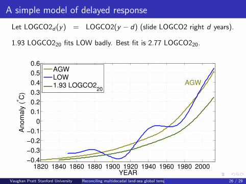
A simple model of delayed response

Let LOGCO2d(y) = LOGCO2(y − d) (slide LOGCO2 right d years).

1.93 LOGCO220 fits LOW badly. Best fit is 2.77 LOGCO220.

1820 1840 1860 1880 1900 1920 1940 1960 1980 2000−0.4

−0.3

−0.2

−0.1

0

0.1

0.2

0.3

0.4

0.5

0.6

YEAR

An

om

aly

(°C

)

AGW

AGWLOW1.93 LOGCO2

20

Vaughan Pratt Stanford University Reconciling multidecadal land-sea global temperature with rising CO2 26 / 29

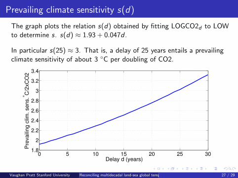
Prevailing climate sensitivity s(d)

The graph plots the relation s(d) obtained by fitting LOGCO2d to LOWto determine s. s(d) ≈ 1.93 + 0.047d .

In particular s(25) ≈ 3. That is, a delay of 25 years entails a prevailingclimate sensitivity of about 3 ◦C per doubling of CO2.

0 5 10 15 20 25 301.8

2

2.2

2.4

2.6

2.8

3

3.2

3.4

Pre

va

ilin

g c

lim.

se

ns. °

C/2

xC

O2

Delay d (years)

Vaughan Pratt Stanford University Reconciling multidecadal land-sea global temperature with rising CO2 27 / 29

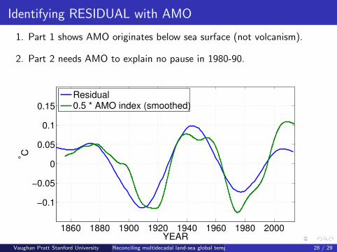
Identifying RESIDUAL with AMO

1. Part 1 shows AMO originates below sea surface (not volcanism).

2. Part 2 needs AMO to explain no pause in 1980-90.

1860 1880 1900 1920 1940 1960 1980 2000

−0.1

−0.05

0

0.05

0.1

0.15

YEAR

°C

Residual0.5 * AMO index (smoothed)

Vaughan Pratt Stanford University Reconciling multidecadal land-sea global temperature with rising CO2 28 / 29

Conclusions

Our understanding of the CO2 control knob is consistent with

1 The natural rises up to 1940 (seems to be the ocean)

2 The hiatus (the Sun and the AMO together)

3 ECS of 3 ◦C/2xCO2 under a 25-year ocean delay.

Further points

Volcanos and El Nino/La Nina not necessary in this account.By Occam’s Razor they should not be part of the explanation.(Contrapositive: If they should be, that refutes Occam’s Razor.)

The more stable human influences besides CO2 are in LOW.This confounds them with CO2, hence a major source of uncertainty.For this reason they have been closely studied for decades.

Vaughan Pratt Stanford University Reconciling multidecadal land-sea global temperature with rising CO2 29 / 29