Recommendation ITU-R P.533-14 (08/2019)

Method for the prediction of the performance of HF circuits

P Series

Radiowave propagation

ii Rec. ITU-R P.533-14

Foreword

The role of the Radiocommunication Sector is to ensure the rational, equitable, efficient and economical use of the radio-

frequency spectrum by all radiocommunication services, including satellite services, and carry out studies without limit

of frequency range on the basis of which Recommendations are adopted.

The regulatory and policy functions of the Radiocommunication Sector are performed by World and Regional

Radiocommunication Conferences and Radiocommunication Assemblies supported by Study Groups.

Policy on Intellectual Property Right (IPR)

ITU-R policy on IPR is described in the Common Patent Policy for ITU-T/ITU-R/ISO/IEC referenced in Resolution

ITU-R 1. Forms to be used for the submission of patent statements and licensing declarations by patent holders are

available from http://www.itu.int/ITU-R/go/patents/en where the Guidelines for Implementation of the Common Patent

Policy for ITU-T/ITU-R/ISO/IEC and the ITU-R patent information database can also be found.

Series of ITU-R Recommendations

(Also available online at http://www.itu.int/publ/R-REC/en)

Series Title

BO Satellite delivery

BR Recording for production, archival and play-out; film for television

BS Broadcasting service (sound)

BT Broadcasting service (television)

F Fixed service

M Mobile, radiodetermination, amateur and related satellite services

P Radiowave propagation

RA Radio astronomy

RS Remote sensing systems

S Fixed-satellite service

SA Space applications and meteorology

SF Frequency sharing and coordination between fixed-satellite and fixed service systems

SM Spectrum management

SNG Satellite news gathering

TF Time signals and frequency standards emissions

V Vocabulary and related subjects

Note: This ITU-R Recommendation was approved in English under the procedure detailed in Resolution ITU-R 1.

Electronic Publication

Geneva, 2019

ITU 2019

All rights reserved. No part of this publication may be reproduced, by any means whatsoever, without written permission of ITU.

Rec. ITU-R P.533-14 1

RECOMMENDATION ITU-R P.533-14

Method for the prediction of the performance of HF circuits*

(1978-1982-1990-1992-1994-1995-1999-2001-2005-2007-2009-2012-2013-2015-2019)

Scope

This Recommendation provides a method for the prediction of available frequencies, of signal levels and of

the predicted reliability for both analogue and digital modulated systems at HF, taking into account not only

the signal-to-noise ratio but also the expected time and frequency spreads of the channel.

Keywords

Ionosphere, HF, prediction

The ITU Radiocommunication Assembly,

considering

a) that tests against ITU-R Data Bank D1 show that the method of Annex 1 of this

Recommendation has comparable accuracy to the other more complex methods;

b) that information on the performance characteristics of transmitting and receiving antennas is

required for the practical application of this method1,

recommends

1 that the information contained in Annex 1 should be used for the prediction of sky-wave

propagation at frequencies between 2 and 30 MHz;

2 that administrations and ITU-R should endeavour to improve prediction methods to enhance

operational facilities and to improve accuracy.

* A computer program (ITURHFProp) associated with the prediction procedures described in this

Recommendation is available from that part of the ITU-R website dealing with Radiocommunication Study

Group 3.

1 Detailed information on a range of antennas with an associated computer program is available from the

ITU; for details, see Recommendation ITU-R BS.705.

2 Rec. ITU-R P.533-14

Annex 1

Table of Contents

Page

1 Introduction .................................................................................................................... 4

PART 1 – Frequency availability............................................................................................. 4

2 Location of control points............................................................................................... 4

3 Basic and operational maximum usable frequencies ...................................................... 4

3.1 Basic maximum usable frequencies .................................................................... 4

3.2 E-layer critical frequency (foE) .......................................................................... 4

3.3 E-layer basic MUF .............................................................................................. 6

3.4 F2-layer characteristics ....................................................................................... 6

3.5 F2-layer basic MUF ............................................................................................ 6

3.6 Within the month probability of ionospheric propagation support .................... 7

3.7 The path operational MUF .................................................................................. 8

4 E-layer maximum screening frequency (fs) .................................................................... 8

PART 2 – Median sky-wave field strength .............................................................................. 9

5 Median sky-wave field strength ..................................................................................... 9

5.1 Elevation angle ................................................................................................... 9

5.2 Paths up to 9 000 km .......................................................................................... 11

5.3 Paths longer than 7 000 km ................................................................................ 16

5.4 Paths between 7 000 and 9 000 km .................................................................... 20

6 Median available receiver power .................................................................................... 21

PART 3 – The prediction of system performance ................................................................... 22

7 Monthly median signal-to-noise ratio............................................................................. 22

8 Sky-wave field strength, available receiver signal power and signal-to-noise ratios

for other percentages of time .......................................................................................... 22

9 Lowest usable frequency (LUF) ..................................................................................... 23

Rec. ITU-R P.533-14 3

Page

10 Basic circuit reliability (BCR) ........................................................................................ 23

10.1 The reliability of analogue modulated systems .................................................. 23

10.2 The reliability of digitally modulated systems, taking account of the time and

frequency spreading of the received signal ........................................................ 23

10.3 Equatorial scattering ........................................................................................... 24

Attachment 1 to Annex 1 – A model for equatorial scattering of HF signals.......................... 25

4 Rec. ITU-R P.533-14

1 Introduction

This prediction procedure applies a ray-path analysis for path lengths up to 7 000 km, composite mode

empirical formulations from the fit to measured data beyond 9 000 km and a smooth transition

between these two approaches over the 7 000-9 000 km distance range.

Monthly median basic MUF, incident sky-wave field strength and available receiver power from a

lossless receiving antenna of given gain are determined. The method includes an estimation of the

parameters of the channel transfer function for use for the prediction of performance of digital

systems. Methods are given for the assessment of circuit reliability. Signal strengths are standardized

against an ITU-R measurement data bank. The method requires the determination of a number of

ionospheric characteristics and propagation parameters at specified “control points”.

In equatorial regions, in the evening hours (local time), it is possible to have distortions in the

predicted results due to regional ionospheric structural instabilities which are not fully accounted for

by this method.

PART 1

Frequency availability

2 Location of control points

Propagation is assumed to be along the great-circle path between the transmitter and receiver

locations via E modes (up to 4 000 km range) and F2 modes (for all distances). Depending on path

length and reflecting layer, control points are selected as indicated in Table 1.

3 Basic and operational maximum usable frequencies

The estimation of operational MUF, the highest frequency that would permit acceptable operation of

a radio service, is in two stages: first, the estimation of basic MUF from a consideration of ionospheric

parameters and second, the determination of a correction factor to allow for propagation mechanisms

at frequencies above the basic MUF.

3.1 Basic maximum usable frequencies

The basic MUFs of the various propagation modes are evaluated in terms of the corresponding

ionospheric layer critical frequencies and a factor related to hop length. Where both E and F2 modes

are considered the higher of the two basic MUFs of the lowest-order E and F2 modes give the basic

MUF for the path.

3.2 E-layer critical frequency (foE)

The monthly median foE is determined as defined in Recommendation ITU-R P.1239.

Rec. ITU-R P.533-14 5

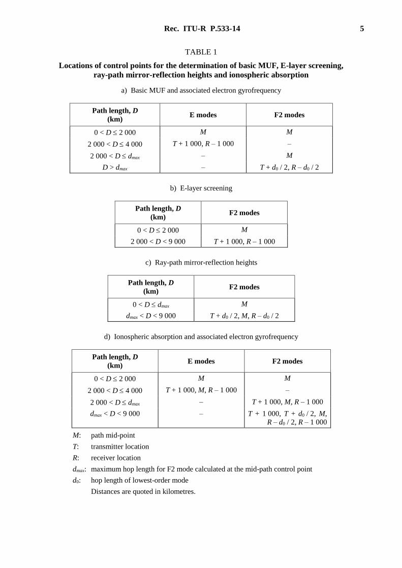
TABLE 1

Locations of control points for the determination of basic MUF, E-layer screening,

ray-path mirror-reflection heights and ionospheric absorption

a) Basic MUF and associated electron gyrofrequency

Path length, D

(km) E modes F2 modes

0 < D 2 000 M M

2 000 < D 4 000 T + 1 000, R – 1 000 –

2 000 < D dmax – M

D > dmax – T + d0 / 2, R – d0 / 2

b) E-layer screening

Path length, D

(km) F2 modes

0 < D 2 000 M

2 000 < D < 9 000 T + 1 000, R – 1 000

c) Ray-path mirror-reflection heights

Path length, D

(km) F2 modes

0 < D dmax M

dmax < D < 9 000 T + d0 / 2, M, R – d0 / 2

d) Ionospheric absorption and associated electron gyrofrequency

Path length, D

(km) E modes F2 modes

0 < D 2 000 M M

2 000 < D 4 000 T + 1 000, M, R – 1 000 –

2 000 < D dmax – T + 1 000, M, R – 1 000

dmax < D < 9 000 – T + 1 000, T + d0 / 2, M,

R – d0 / 2, R – 1 000

M: path mid-point

T: transmitter location

R: receiver location

dmax: maximum hop length for F2 mode calculated at the mid-path control point

d0: hop length of lowest-order mode

Distances are quoted in kilometres.

6 Rec. ITU-R P.533-14

3.3 E-layer basic MUF

foE is evaluated at the control points noted in Table 1a) and for path lengths of 2 000-4 000 km the

lower value is selected. The basic MUF of an n-hop E mode over a path of length D is given by:

110secfoEMUF)(E iDn (1)

where i110 is the angle of incidence at a mid-hop mirror-reflection height of 110 km for a hop of length

d = D/n.

The E-layer basic MUF for the path is the value of n0E(D)MUF for the lowest-order E-mode, n0.

3.4 F2-layer characteristics

Numerical representations of the monthly median ionospheric characteristics foF2 and M(3000)F2,

for solar-index values R12 = 0 and 100, and for each month are taken from

Recommendation ITU-R P.1239 where the magnetic field is evaluated at a height of 300 km. These

representations are used to determine these values for the required times and for the control points

given in Table 1a). Linear interpolation or extrapolation is applied for the prevailing index values

between R12 = 0 and 160 (see Recommendation ITU-R P.371). For higher sunspot activity, R12 is set

equal to 160 in the case of foF2 only.

3.5 F2-layer basic MUF

3.5.1 Lowest-order mode

3.5.1.1 Paths up to dmax (km)

The lowest-order mode, n0, is determined by geometrical considerations, using the mirror reflection

height hr derived at the mid-path control point from the equation:

2)3000(

4901

FMhr 176 km or 500 km, whichever is the smaller (2)

For the nth order mode, the F2-layer basic MUF is calculated as:

xam

Hd

d

dffoFB

C

CMUFDFn 1

22)1(1)(2

3000

(3)

where:

fH : value of electron gyrofrequency, for a height of 300 km, determined at each of

the appropriate control points given in Table 1a)

Cd = 0.74 – 0.591 Z – 0.424 Z2 – 0.090 Z3 + 0.088 Z4 + 0.181 Z5 + 0.096 Z6 (4)

with Z = 1 – 2d / dmax

dmax = 4 780 + (12 610 + 2 140 / x2 – 49 720 / x4 + 688 900 / x6) (1 / B – 0.303) (5)

96351

8547sin005002150]4]2)3000([[12402)3000( 2 .–

x

...–FM.–FMB (6)

Rec. ITU-R P.533-14 7

where:

d : D/n and dmax are in kilometres

C3000 : value of Cd for d = 3 000 km

x : foF2/foE, or 2, whichever is the larger

foE is calculated as in § 3.2.

The nF2(D)MUF for the lowest-order mode, n0, is the path basic MUF. For the calculation of the

basic MUF dmax is restricted to be no greater than 4 000 km.

3.5.1.2 Paths longer than dmax (km)

The basic MUF of the lowest-order mode n0 F2(D)MUF for path length D is taken equal to the lower

of the F2(dmax)MUF values determined from equation (3) for the two control points given in

Table 1a). This is also the basic MUF for the path.

3.5.2 Higher-order modes (paths up to 9 000 km)

3.5.2.1 Paths up to dmax (km)

The F2-layer basic MUF for an n-hop mode is calculated using equations (3) to (6) at the midpath

control point given in Table 1a) for hop length d = D/n.

3.5.2.2 Paths longer than dmax (km)

The F2-layer basic MUF for an n-hop mode is calculated in terms of F2(dmax)MUF and a distance

scaling factor dependent on the respective hop lengths of the mode in question and the lowest possible

order mode. For the calculation of Mn and Mn0, the maximum hop distance, dmax, is recalculated at the

control point and can be larger than 4 000 km.

0

)(2)(2 0 nnmax M/MMUFdFnMUFDFn (7)

where Mn/Mn0 is derived using equation (3) as follows:

MUFDFn

MUFDnF

M

M

n

n

)(2

)(2

00

(8)

The lower of the values calculated at the two control points of Table 1a) is selected.

3.6 Within the month probability of ionospheric propagation support

In some cases, it may be sufficient to predict the probability of having sufficient ionization to support

propagation over the path, without taking into account system and antenna characteristics and

performance requirements. In such cases, the probability that the MUF exceeds the working

frequency is required. Sections 3.3 and 3.5 above give the median values of MUF(50) for E and F2

propagation.

For F2 modes, the lower decile ratio, δl, of the MUF exceeded for 90% of the days of the month,

MUF(90), to MUF(50) is given in Recommendation ITU-R P.1239, Table 2, as a function of local

time, latitude, season and sunspot number.

For cases where the working frequency, f, is less than MUF(50), the probability of ionospheric

support is given by:

𝐹𝑝𝑟𝑜𝑏 = 1.3 −0.8

1+ {1− [

𝑓MUF(50)⁄ ]

1−δ𝑙}

or = 1, whichever is the smaller (9)

8 Rec. ITU-R P.533-14

The upper decile ratio, δu, of the MUF exceeded for 10% of the days of the month, MUF(10) to

MUF(50) is given in Recommendation ITU-R P.1239, Table 3, as a function of local time, latitude,

season and sunspot number.

For cases where the working frequency, f, is greater than MUF(50), the probability of ionospheric

support is given by:

𝐹𝑝𝑟𝑜𝑏 =0.8

1+ { [

𝑓MUF(50)⁄ ]−1

δ𝑢−1}

− 0.3 or = 0, whichever is the larger (10)

In the case of E modes, the appropriate factors for the interdecile range are 1.05 and 0.95, respectively.

The distribution of the operational MUF at a given hour within a month may be obtained by applying

the distribution given in § 3.6.

Note that the operational MUFs exceeded for 90% and 10% of days of the month are defined as the

optimum working frequency and the highest probable frequency respectively.

3.7 The path operational MUF

The path operational MUF is the greater of the operational MUF for F2 modes and the operational

MUF for E modes. The relationship between the operational and basic MUFs will depend on the

systems and antenna characteristics and on the path length geographic and other considerations, and

should be determined from practical experience of the circuit performance. Where this experience is

not available, for F2 modes, the operational MUF = basic MUF. Rop where Rop is given in Table 1 to

Recommendation ITU-R P.1240; for E modes the operational MUF is equal to the basic MUF.

An estimate of the operational MUF exceeded for 10% and 90% of the days is determined by

multiplying the median operational MUF by the appropriate factors given in Recommendation ITU-R

P.1239, Tables 2 and 3, in the case of the F modes. In the case of E modes the appropriate factors are

1.05 and 0.95 respectively.

4 E-layer maximum screening frequency (fs)

E-layer screening of F2 modes is considered for paths up to 4 000 km (see Table 1b). The foE value

at the path mid-point (for paths up to 2 000 km), or the higher one of the foE values at the two control

points 1 000 km from each end of the path (for paths longer than 2 000 km), is taken for the calculation

of the maximum screening frequency.

fs = 1.05 foE sec i (11)

with:

r

F

hR

R

0

0 cosarcsini (12)

where:

i : angle of incidence at height hr = 110 km

R0 : radius of the Earth, 6 371 km

F : elevation angle for the F2-layer mode (determined from equation (13)).

Rec. ITU-R P.533-14 9

PART 2

Median sky-wave field strength

5 Median sky-wave field strength

The predicted field strength is the monthly median over all days of the month. The prediction

procedure is in three parts, dependent on the path length. For path distances less than 7 000 km

predictions of median sky-wave field strength are made using only the method given in § 5.2. For

path distances greater than 9 000 km median sky-wave field strengths are made using only the method

given in § 5.3. For path distances between 7 000 and 9 000 km both methods are used and the results

are interpolated by the method described in § 5.4.

5.1 Elevation angle

The elevation angle which applies for all frequencies, including those above the basic MUF, is given

by:

00

0

0 2cosec

2cotarctan

R

d

hR

R–

R

d

r

(13)

where:

d : hop length of an n-hop mode given by d = D/n

hr : equivalent plane-mirror reflection height

for E modes hr = 110 km

for F2 modes hr is taken as a function of time, location and hop length.

The mirror reflection height for F2 modes, hr, is calculated as follows, where:

x = foF2/foE and 316–2F)3000(M

4901

MH

with:

150

)25–(096.0

4.1–

18.0 12R

yM

and y = x or 1.8, whichever is the larger.

a) For x > 3.33 and xr = f / foF2 1, where f is the wave frequency:

hr = h or 800 km, whichever is the smaller (14)

where:

h = A1 + B1 2.4–a for B1 and a 0

= A1 + B1 otherwise

with:

A1 = 140 + (H – 47) E1

B1 = 150 + (H – 17) F1 – A1

E1 = –0.09707 3rx + 0.6870

2rx – 0.7506 xr + 0.6

10 Rec. ITU-R P.533-14

F1 is such that:

F1 = –1.862 4rx + 12.95

3rx – 32.03

2rx + 33.50 xr – 10.91 for xr 1.71

F1 = 1.21 + 0.2 xr for xr > 1.71

and a varies with distance d and skip distance ds as:

a = (d – ds) / (H + 140)

where:

ds = 160 + (H + 43) G

G = –2.102 4rx + 19.50

3rx – 63.15

2rx + 90.47 xr – 44.73 for xr 3.7

G = 19.25 for xr > 3.7

b) For x > 3.33 and xr < 1:

hr = h or 800 km, whichever is the smaller (15)

where:

h = A2 + B2 b for B2 0

= A2 + B2 otherwise

with:

A2 = 151 + (H – 47) E2

B2 = 141 + (H – 24) F2 – A2

E2 = 0.1906 Z2 + 0.00583 Z + 0.1936

F2 = 0.645 Z

2 + 0.883 Z + 0.162

where:

Z = xr or 0.1, whichever is the larger and b varies with normalized distance df,

Z and H as follows:

b = –7.535 4fd + 15.75

3fd – 8.834

2fd – 0.378 df + 1

where:

140

1150

HZ

d.df or 0.65; whichever is the smaller

c) For x 3.33:

hr = 115 + H J + U d or 800 km, whichever is the smaller (16)

with:

J = – 0.7126 y3 + 5.863 y2 – 16.13 y + 16.07

and

U = 8 10–5 (H – 80) (1 + 11 y–2.2) + 1.2 10–3 H y–3.6

In the case of paths up to dmax (km), hr is evaluated at the path mid-point: for longer paths, it is

determined for all the control points given in Table 1c) and the mean value is used.

Rec. ITU-R P.533-14 11

5.2 Paths up to 9 000 km

For path distances less than 7 000 km predictions of median sky-wave field strength are made using

only the method given in § 5.2. For path distances between 7 000 and 9 000 km both methods in

§§ 5.2 and 5.3 are used. The results from each method are then interpolated by the method given in

§ 5.4.

5.2.1 Modes considered

Up to three E modes (for paths up to 4 000 km) and up to six F2 modes are selected, each of which

meets all of the following separate criteria:

– mirror-reflection heights:

• for E modes, from a height hr = 110 km;

• for F2 modes, from a height hr determined from equation (2), where M(3000)F2 is

evaluated at the mid-path control point (path lengths up to dmax (km)), or at the control

point given in Table 1c) for which foF2 has the lower value (path lengths from dmax to

9 000 km);

– E modes – the lowest-order mode with hop length up to 2 000 km, and the next two

higher-order modes;

– F2 modes – the lowest-order mode with a hop length up to dmax (km) and the next five higher-

order modes, which have an E-layer maximum screening frequency evaluated as described

in § 4 which is less than the operating frequency.

5.2.2 Field strength determination

For each mode w selected in § 5.2.1, the median field strength is given by:

Ew = 136.6 + Pt + Gt + 20 log f – Lb dB(1 V/m) (17)

where:

f : transmitting frequency (MHz)

Pt : transmitter power (dB(1 kW))

Gt : transmitting antenna gain at the required azimuth angle and elevation angle ()

relative to an isotropic antenna (dB)

Lb : the ray path basic transmission loss for the mode under consideration given by:

Lb = 32.45 + 20 log f + 20 log p + Li + Lm + Lg + Lh + Lz (18)

with:

p: virtual slant range (km)

n

Rd/

Rd/Rp

1 0

00

2Δcos

2sin2 (19)

Li: the absorption loss (dB) for an n-hop mode is given in equation (20) which is

calculated at m penetration points. The penetration points are determined by

assuming a fixed reflection height of 300 km and a penetration height of 90 km

(two penetration points per hop).

12 21

( χ )1 0.0067 sec

(χ ) foE

mjnoon j v

i njnoon jj Lj

AT F fL R i

Ff f

(20)

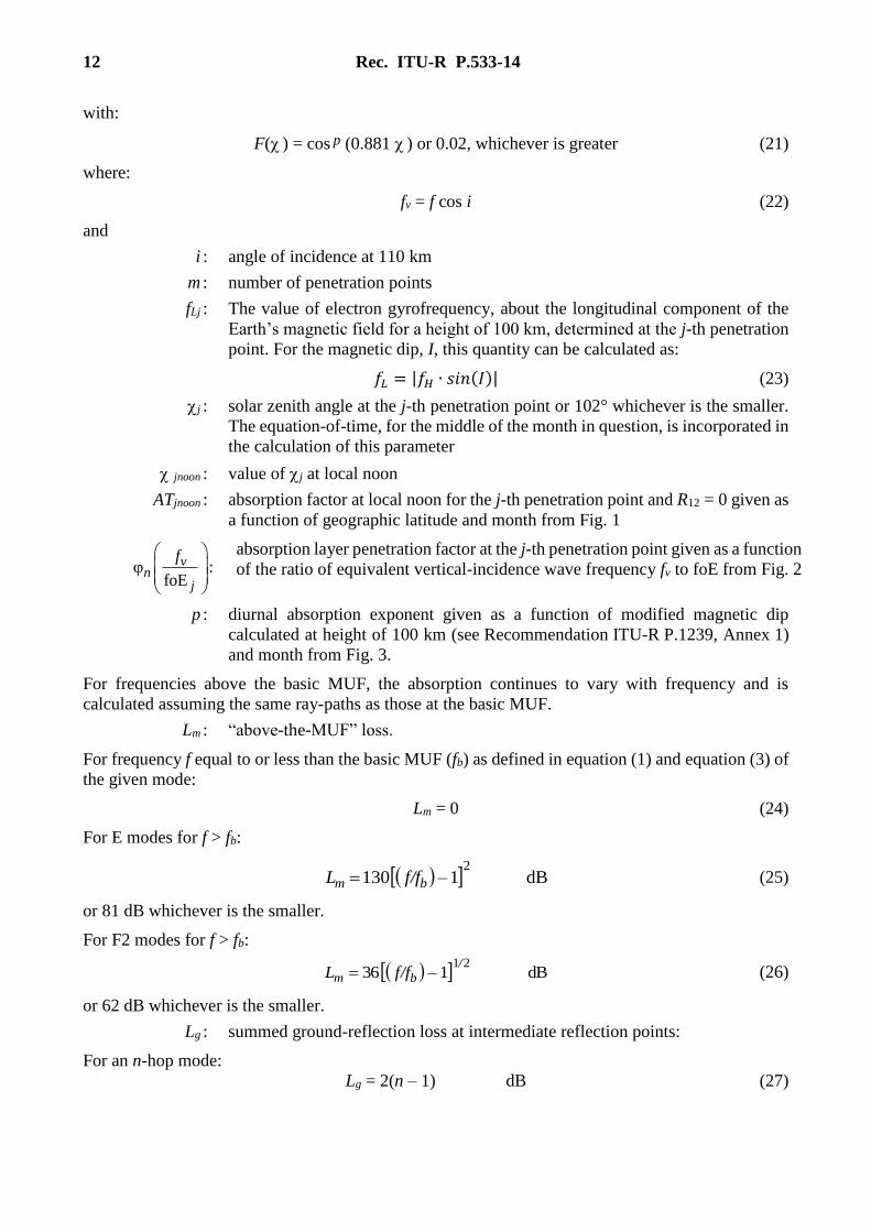
12 Rec. ITU-R P.533-14

with:

F( ) = cos p (0.881 ) or 0.02, whichever is greater (21)

where:

fv = f cos i (22)

and

i : angle of incidence at 110 km

m : number of penetration points

fLj : The value of electron gyrofrequency, about the longitudinal component of the

Earth’s magnetic field for a height of 100 km, determined at the j-th penetration

point. For the magnetic dip, I, this quantity can be calculated as:

𝑓𝐿 = |𝑓𝐻 ∙ 𝑠𝑖𝑛(𝐼)| (23)

j : solar zenith angle at the j-th penetration point or 102° whichever is the smaller.

The equation-of-time, for the middle of the month in question, is incorporated in

the calculation of this parameter

jnoon : value of j at local noon

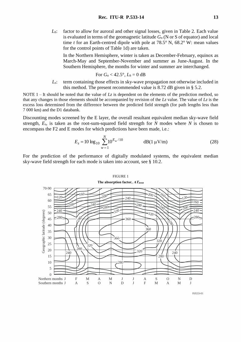
ATjnoon : absorption factor at local noon for the j-th penetration point and R12 = 0 given as

a function of geographic latitude and month from Fig. 1

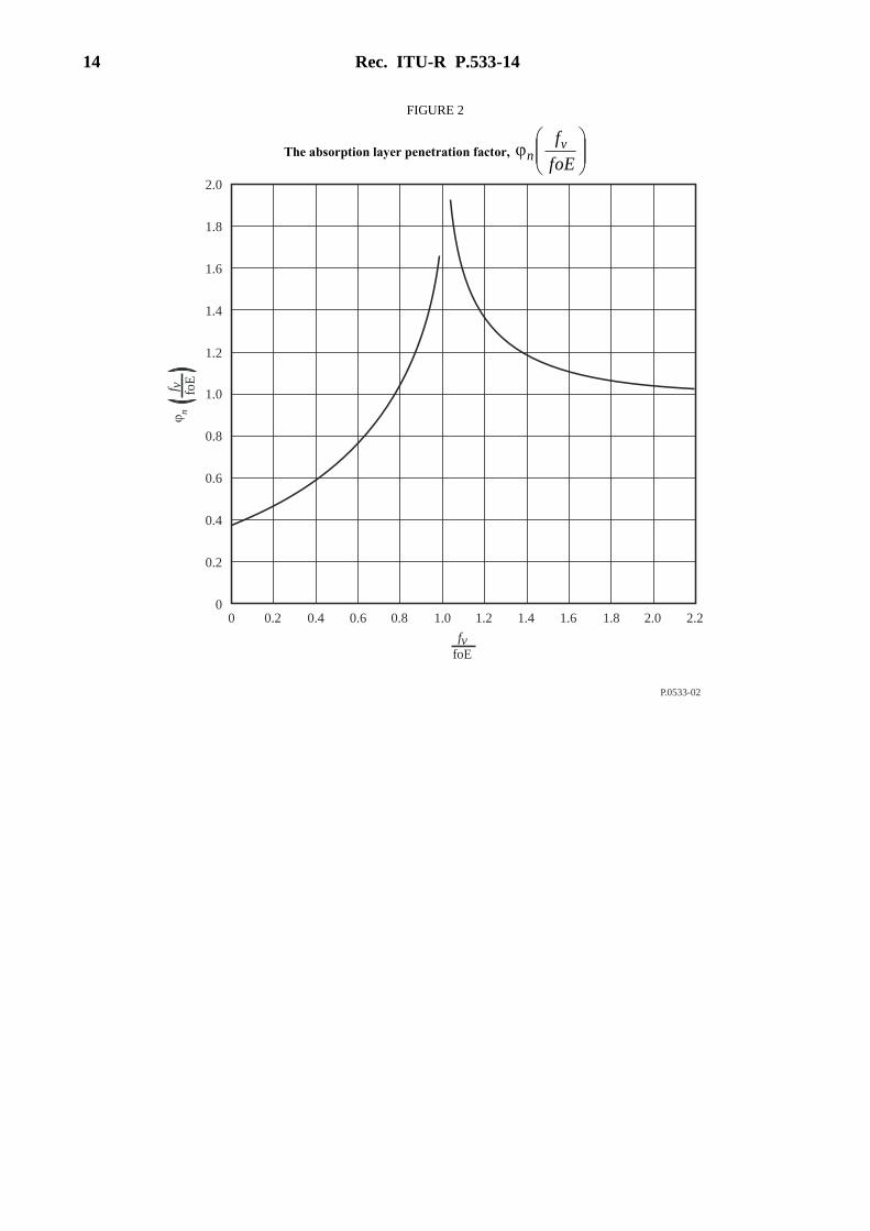
:foE

vn

j

f

absorption layer penetration factor at the j-th penetration point given as a function

of the ratio of equivalent vertical-incidence wave frequency fv to foE from Fig. 2

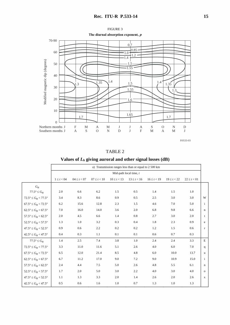
p : diurnal absorption exponent given as a function of modified magnetic dip

calculated at height of 100 km (see Recommendation ITU-R P.1239, Annex 1)

and month from Fig. 3.

For frequencies above the basic MUF, the absorption continues to vary with frequency and is

calculated assuming the same ray-paths as those at the basic MUF.

Lm : “above-the-MUF” loss.

For frequency f equal to or less than the basic MUF (fb) as defined in equation (1) and equation (3) of

the given mode:

Lm = 0 (24)

For E modes for f > fb:

dB11302

–f/fL bm (25)

or 81 dB whichever is the smaller.

For F2 modes for f > fb:

dB13621/

bm –f/fL (26)

or 62 dB whichever is the smaller.

Lg : summed ground-reflection loss at intermediate reflection points:

For an n-hop mode:

Lg = 2(n – 1) dB (27)

Rec. ITU-R P.533-14 13

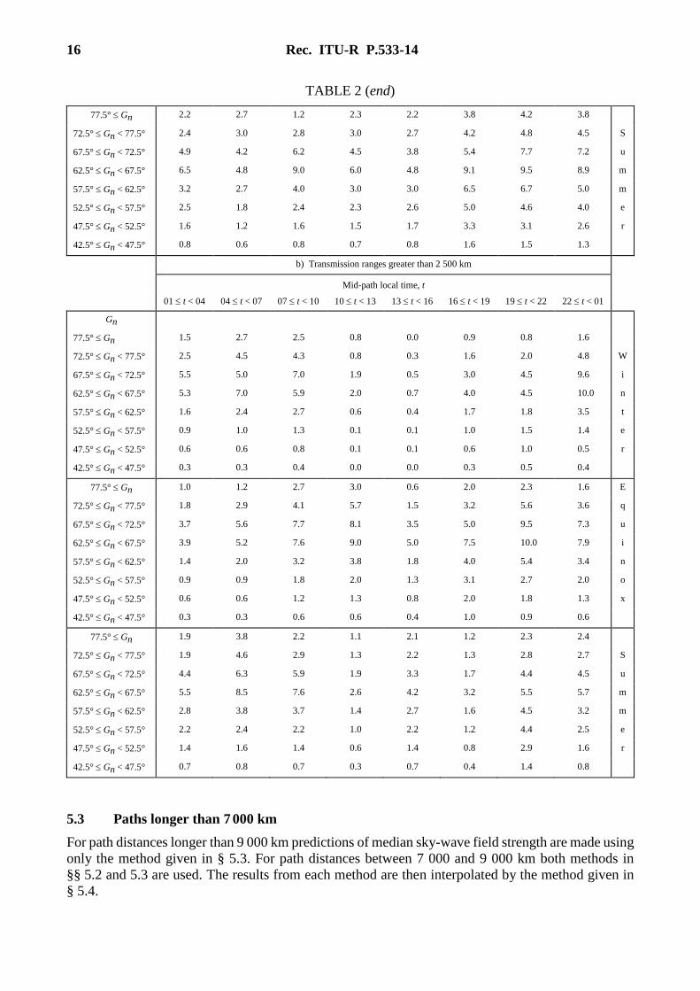
Lh: factor to allow for auroral and other signal losses, given in Table 2. Each value

is evaluated in terms of the geomagnetic latitude Gn (N or S of equator) and local

time t for an Earth-centred dipole with pole at 78.5° N, 68.2° W: mean values

for the control points of Table 1d) are taken.

In the Northern Hemisphere, winter is taken as December-February, equinox as

March-May and September-November and summer as June-August. In the

Southern Hemisphere, the months for winter and summer are interchanged.

For Gn < 42.5°, Lh = 0 dB

Lz: term containing those effects in sky-wave propagation not otherwise included in

this method. The present recommended value is 8.72 dB given in § 5.2.

NOTE 1 – It should be noted that the value of Lz is dependent on the elements of the prediction method, so

that any changes in those elements should be accompanied by revision of the Lz value. The value of Lz is the

excess loss determined from the difference between the predicted field strength (for path lengths less than

7 000 km) and the D1 databank.

Discounting modes screened by the E layer, the overall resultant equivalent median sky-wave field

strength, Es, is taken as the root-sum-squared field strength for N modes where N is chosen to

encompass the F2 and E modes for which predictions have been made, i.e.:

N

w

Es

wE1

10/10 10log10 dB(1 V/m) (28)

For the prediction of the performance of digitally modulated systems, the equivalent median

sky-wave field strength for each mode is taken into account, see § 10.2.

FIGURE 1

The absorption factor, ATnoon

P.0533-01

Geo

gra

phi

c la

titu

de

(deg

rees

)

JJ

FA

MS

AO

MN

JD

JJ

AF

SM

OA

NM

DJ

Northern monthsSouthern months

70-90

65

60

55

50

45

40

35

30

25

20

15

10

0

5

240200

240

160240

240

320

360

360

320

240280

200

200

160

280280

200

280

280

120

160

280

320

240

360

280240

320

120

280

320

280

14 Rec. ITU-R P.533-14

FIGURE 2

The absorption layer penetration factor,

foE

fvn

P.0533-02

0

0.2

0.4

0.6

0.8

0

1.2

1.4

1.6

1.8

2.0

1.

0 0.2 0.4 0.6 0.8 1.0 1.2 1.4 1.6 1.8 2.0 2.2

fvfoE

n

f v foE

Rec. ITU-R P.533-14 15

FIGURE 3

The diurnal absorption exponent, p

P.0533-03

1.41.41.351.3

0.7

0.851.0

1.2

1.5

1.55

1.5

1.55

1.6

1.65

1.4

1.7 1.7

1.3

1.35

Modif

ied m

agn

etic

dip

(d

egre

es)

JJ

FA

MS

AO

MN

JD

JJ

AF

SM

OA

NM

DJ

Northern monthsSouthern months

70-90

60

50

40

30

20

10

0

TABLE 2

Values of Lh giving auroral and other signal losses (dB)

a) Transmission ranges less than or equal to 2 500 km

Mid-path local time, t

1 t < 04 04 t < 07 07 t < 10 10 t < 13 13 t < 16 16 t < 19 19 t < 22 22 t < 01

Gn

77.5° Gn 2.0 6.6 6.2 1.5 0.5 1.4 1.5 1.0

72.5° Gn < 77.5° 3.4 8.3 8.6 0.9 0.5 2.5 3.0 3.0 W

67.5° Gn < 72.5° 6.2 15.6 12.8 2.3 1.5 4.6 7.0 5.0 i

62.5° Gn < 67.5° 7.0 16.0 14.0 3.6 2.0 6.8 9.8 6.6 n

57.5° Gn < 62.5° 2.0 4.5 6.6 1.4 0.8 2.7 3.0 2.0 t

52.5° Gn < 57.5° 1.3 1.0 3.2 0.3 0.4 1.8 2.3 0.9 e

47.5° Gn < 52.5° 0.9 0.6 2.2 0.2 0.2 1.2 1.5 0.6 r

42.5° Gn < 47.5° 0.4 0.3 1.1 0.1 0.1 0.6 0.7 0.3

77.5° Gn 1.4 2.5 7.4 3.8 1.0 2.4 2.4 3.3 E

72.5° Gn < 77.5° 3.3 11.0 11.6 5.1 2.6 4.0 6.0 7.0 q

67.5° Gn < 72.5° 6.5 12.0 21.4 8.5 4.8 6.0 10.0 13.7 u

62.5° Gn < 67.5° 6.7 11.2 17.0 9.0 7.2 9.0 10.9 15.0 i

57.5° Gn < 62.5° 2.4 4.4 7.5 5.0 2.6 4.8 5.5 6.1 n

52.5° Gn < 57.5° 1.7 2.0 5.0 3.0 2.2 4.0 3.0 4.0 o

47.5° Gn < 52.5° 1.1 1.3 3.3 2.0 1.4 2.6 2.0 2.6 x

42.5° Gn < 47.5° 0.5 0.6 1.6 1.0 0.7 1.3 1.0 1.3

16 Rec. ITU-R P.533-14

TABLE 2 (end)

77.5° Gn 2.2 2.7 1.2 2.3 2.2 3.8 4.2 3.8

72.5° Gn < 77.5° 2.4 3.0 2.8 3.0 2.7 4.2 4.8 4.5 S

67.5° Gn < 72.5° 4.9 4.2 6.2 4.5 3.8 5.4 7.7 7.2 u

62.5° Gn < 67.5° 6.5 4.8 9.0 6.0 4.8 9.1 9.5 8.9 m

57.5° Gn < 62.5° 3.2 2.7 4.0 3.0 3.0 6.5 6.7 5.0 m

52.5° Gn < 57.5° 2.5 1.8 2.4 2.3 2.6 5.0 4.6 4.0 e

47.5° Gn < 52.5° 1.6 1.2 1.6 1.5 1.7 3.3 3.1 2.6 r

42.5° Gn < 47.5° 0.8 0.6 0.8 0.7 0.8 1.6 1.5 1.3

b) Transmission ranges greater than 2 500 km

Mid-path local time, t

01 t < 04 04 t < 07 07 t < 10 10 t < 13 13 t < 16 16 t < 19 19 t < 22 22 t < 01

Gn

77.5° Gn 1.5 2.7 2.5 0.8 0.0 0.9 0.8 1.6

72.5° Gn < 77.5° 2.5 4.5 4.3 0.8 0.3 1.6 2.0 4.8 W

67.5° Gn < 72.5° 5.5 5.0 7.0 1.9 0.5 3.0 4.5 9.6 i

62.5° Gn < 67.5° 5.3 7.0 5.9 2.0 0.7 4.0 4.5 10.0 n

57.5° Gn < 62.5° 1.6 2.4 2.7 0.6 0.4 1.7 1.8 3.5 t

52.5° Gn < 57.5° 0.9 1.0 1.3 0.1 0.1 1.0 1.5 1.4 e

47.5° Gn < 52.5° 0.6 0.6 0.8 0.1 0.1 0.6 1.0 0.5 r

42.5° Gn < 47.5° 0.3 0.3 0.4 0.0 0.0 0.3 0.5 0.4

77.5° Gn 1.0 1.2 2.7 3.0 0.6 2.0 2.3 1.6 E

72.5° Gn < 77.5° 1.8 2.9 4.1 5.7 1.5 3.2 5.6 3.6 q

67.5° Gn < 72.5° 3.7 5.6 7.7 8.1 3.5 5.0 9.5 7.3 u

62.5° Gn < 67.5° 3.9 5.2 7.6 9.0 5.0 7.5 10.0 7.9 i

57.5° Gn < 62.5° 1.4 2.0 3.2 3.8 1.8 4.0 5.4 3.4 n

52.5° Gn < 57.5° 0.9 0.9 1.8 2.0 1.3 3.1 2.7 2.0 o

47.5° Gn < 52.5° 0.6 0.6 1.2 1.3 0.8 2.0 1.8 1.3 x

42.5° Gn < 47.5° 0.3 0.3 0.6 0.6 0.4 1.0 0.9 0.6

77.5° Gn 1.9 3.8 2.2 1.1 2.1 1.2 2.3 2.4

72.5° Gn < 77.5° 1.9 4.6 2.9 1.3 2.2 1.3 2.8 2.7 S

67.5° Gn < 72.5° 4.4 6.3 5.9 1.9 3.3 1.7 4.4 4.5 u

62.5° Gn < 67.5° 5.5 8.5 7.6 2.6 4.2 3.2 5.5 5.7 m

57.5° Gn < 62.5° 2.8 3.8 3.7 1.4 2.7 1.6 4.5 3.2 m

52.5° Gn < 57.5° 2.2 2.4 2.2 1.0 2.2 1.2 4.4 2.5 e

47.5° Gn < 52.5° 1.4 1.6 1.4 0.6 1.4 0.8 2.9 1.6 r

42.5° Gn < 47.5° 0.7 0.8 0.7 0.3 0.7 0.4 1.4 0.8

5.3 Paths longer than 7 000 km

For path distances longer than 9 000 km predictions of median sky-wave field strength are made using

only the method given in § 5.3. For path distances between 7 000 and 9 000 km both methods in

§§ 5.2 and 5.3 are used. The results from each method are then interpolated by the method given in

§ 5.4.

Rec. ITU-R P.533-14 17

For paths longer than 7 000 km, calculating all possible modes is impractical. Consequently, the

following method is applied where the LUF (fL) and the operational MUF (fM) define the transmission

frequency range. The values fM and fL are the most important parameters in the empirical formula to

calculate the field strength. However, for path lengths between 7 000 and 9 000 km, the results of the

two methods are interpolated in order to provide a smooth transition (see § 5.4).

This method involves three basic steps:

− determination of the fM;

− determination of the fL;

− estimation of the field strength.

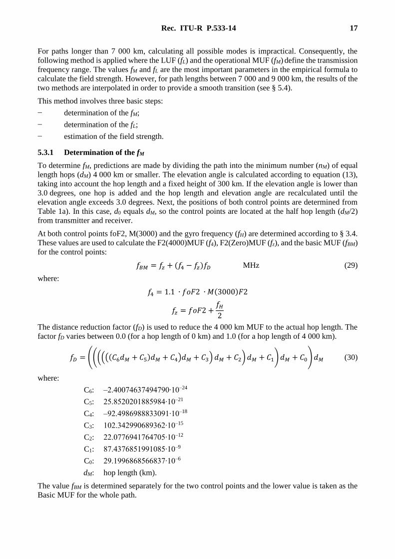
5.3.1 Determination of the fM

To determine fM, predictions are made by dividing the path into the minimum number (nM) of equal

length hops (dM) 4 000 km or smaller. The elevation angle is calculated according to equation (13),

taking into account the hop length and a fixed height of 300 km. If the elevation angle is lower than

3.0 degrees, one hop is added and the hop length and elevation angle are recalculated until the

elevation angle exceeds 3.0 degrees. Next, the positions of both control points are determined from

Table 1a). In this case, d0 equals dM, so the control points are located at the half hop length (dM/2)

from transmitter and receiver.

At both control points foF2, M(3000) and the gyro frequency (fH) are determined according to § 3.4.

These values are used to calculate the F2(4000)MUF (f4), F2(Zero)MUF (fz), and the basic MUF (fBM)

for the control points:

𝑓𝐵𝑀 = 𝑓𝑧 + (𝑓4 − 𝑓𝑧)𝑓𝐷 MHz (29)

where:

𝑓4 = 1.1 ∙ 𝑓𝑜𝐹2 ∙ 𝑀(3000)𝐹2

𝑓𝑧 = 𝑓𝑜𝐹2 +𝑓𝐻

2

The distance reduction factor (fD) is used to reduce the 4 000 km MUF to the actual hop length. The

factor fD varies between 0.0 (for a hop length of 0 km) and 1.0 (for a hop length of 4 000 km).

𝑓𝐷 = ((((((𝐶6𝑑𝑀 + 𝐶5)𝑑𝑀 + 𝐶4)𝑑𝑀 + 𝐶3) 𝑑𝑀 + 𝐶2) 𝑑𝑀 + 𝐶1) 𝑑𝑀 + 𝐶0) 𝑑𝑀 (30)

where:

C6: –2.40074637494790∙10–24

C5: 25.8520201885984∙10–21

C4: –92.4986988833091∙10–18

C3: 102.342990689362∙10–15

C2: 22.0776941764705∙10–12

C1: 87.4376851991085∙10–9

C0: 29.1996868566837∙10–6

dM: hop length (km).

The value fBM is determined separately for the two control points and the lower value is taken as the

Basic MUF for the whole path.

18 Rec. ITU-R P.533-14

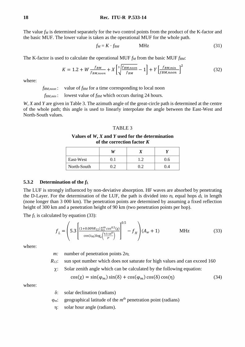
The value fM is determined separately for the two control points from the product of the K-factor and

the basic MUF. The lower value is taken as the operational MUF for the whole path.

fM = K · fBM MHz (31)

The K-factor is used to calculate the operational MUF fM from the basic MUF fBM:

𝐾 = 1.2 + 𝑊𝑓𝐵𝑀

𝑓𝐵𝑀,𝑛𝑜𝑜𝑛+ 𝑋 [√

𝑓𝐵𝑀,𝑛𝑜𝑜𝑛

𝑓𝐵𝑀

3− 1] + 𝑌 [

𝑓𝐵𝑀,𝑚𝑖𝑛

𝑓𝐵𝑀,𝑛𝑜𝑜𝑛]

2

(32)

where:

fBM,noon : value of fBM for a time corresponding to local noon

fBM,min : lowest value of fBM which occurs during 24 hours.

W, X and Y are given in Table 3. The azimuth angle of the great-circle path is determined at the centre

of the whole path; this angle is used to linearly interpolate the angle between the East-West and

North-South values.

TABLE 3

Values of W, X and Y used for the determination

of the correction factor K

W X Y

East-West 0.1 1.2 0.6

North-South 0.2 0.2 0.4

5.3.2 Determination of the fL

The LUF is strongly influenced by non-deviative absorption. HF waves are absorbed by penetrating

the D-Layer. For the determination of the LUF, the path is divided into nL equal hops dL in length

(none longer than 3 000 km). The penetration points are determined by assuming a fixed reflection

height of 300 km and a penetration height of 90 km (two penetration points per hop).

The fL is calculated by equation (33):

𝑓𝐿 = (5.3 [(1+0.009𝑅12) ∑ 𝑐𝑜𝑠0.5(χ)𝑚

1

cos(𝑖90)log𝑒(9.5∙106

𝑝, )

]

0.5

− 𝑓𝐻) (𝐴𝑤 + 1) MHz (33)

where:

m: number of penetration points 2nL

R12: sun spot number which does not saturate for high values and can exceed 160

: Solar zenith angle which can be calculated by the following equation:

cos(χ) = sin(φ𝑚) sin(δ) + cos(φ𝑚) cos(δ) cos (η) (34)

where:

δ: solar declination (radians)

φm: geographical latitude of the mth penetration point (radians)

η: solar hour angle (radians).

Rec. ITU-R P.533-14 19

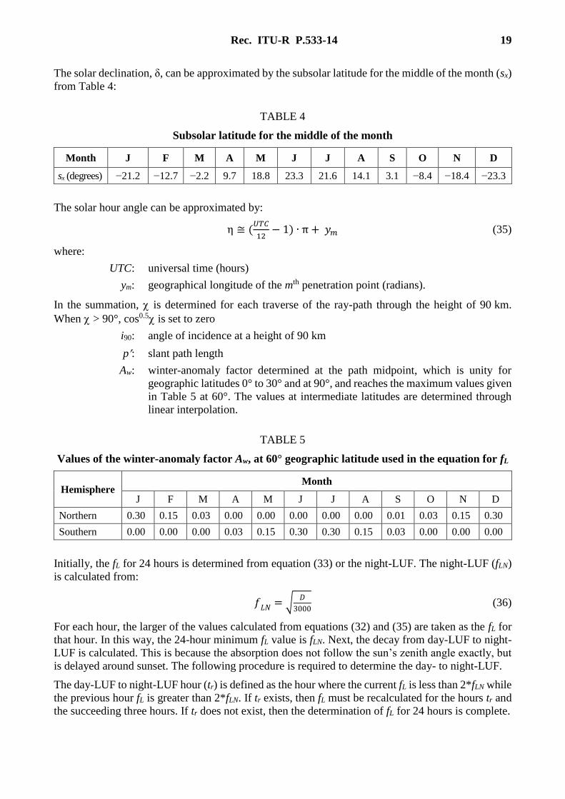
The solar declination, δ, can be approximated by the subsolar latitude for the middle of the month (sx)

from Table 4:

TABLE 4

Subsolar latitude for the middle of the month

Month J F M A M J J A S O N D

sx (degrees) −21.2 −12.7 −2.2 9.7 18.8 23.3 21.6 14.1 3.1 −8.4 −18.4 −23.3

The solar hour angle can be approximated by:

η ≅ (𝑈𝑇𝐶

12− 1) ∙ π + 𝑦𝑚 (35)

where:

UTC: universal time (hours)

ym: geographical longitude of the mth penetration point (radians).

In the summation, is determined for each traverse of the ray-path through the height of 90 km.

When > 90°, cos0.5 is set to zero

i90: angle of incidence at a height of 90 km

p: slant path length

Aw: winter-anomaly factor determined at the path midpoint, which is unity for

geographic latitudes 0° to 30° and at 90°, and reaches the maximum values given

in Table 5 at 60°. The values at intermediate latitudes are determined through

linear interpolation.

TABLE 5

Values of the winter-anomaly factor Aw, at 60° geographic latitude used in the equation for fL

Hemisphere Month

J F M A M J J A S O N D

Northern 0.30 0.15 0.03 0.00 0.00 0.00 0.00 0.00 0.01 0.03 0.15 0.30

Southern 0.00 0.00 0.00 0.03 0.15 0.30 0.30 0.15 0.03 0.00 0.00 0.00

Initially, the fL for 24 hours is determined from equation (33) or the night-LUF. The night-LUF (fLN)

is calculated from:

𝑓𝐿𝑁 = √𝐷

3000 (36)

For each hour, the larger of the values calculated from equations (32) and (35) are taken as the fL for

that hour. In this way, the 24-hour minimum fL value is fLN. Next, the decay from day-LUF to night-

LUF is calculated. This is because the absorption does not follow the sun’s zenith angle exactly, but

is delayed around sunset. The following procedure is required to determine the day- to night-LUF.

The day-LUF to night-LUF hour (tr) is defined as the hour where the current fL is less than 2*fLN while

the previous hour fL is greater than 2*fLN. If tr exists, then fL must be recalculated for the hours tr and

the succeeding three hours. If tr does not exist, then the determination of fL for 24 hours is complete.

20 Rec. ITU-R P.533-14

When tr exists, the fL for that hour and the succeeding three hours must be recalculated in the following

way. For the hour (tr), fL is calculated using:

𝑓𝐿(𝑡𝑟) = 𝑒−0.23 ∙ 𝑓𝐿(𝑡𝑟 − 1) ∙ (𝑑𝑡 ∙ (1 − 𝑒−0.23) + 𝑒−0.23) (37)

where:

𝑑𝑡 =2 ∙ 𝑓𝐿𝑁 − 𝑓𝐿(𝑡𝑟)

𝑓𝐿(𝑡𝑟 − 1) − 𝑓𝐿(𝑡𝑟)

For the succeeding three hours (n = 1, 2 and 3), fL is calculated by:

𝑓𝐿(𝑡𝑟 + 𝑛) = 𝑓𝐿(𝑡𝑟 + 𝑛 − 1) ∙ 𝑒−0.23 (38)

The newly recalculated fL values replace the initial fL values only if they are larger. Once all fL values

in a 24-hour period are calculated, the current hour fL value is selected and the fL calculation is

complete.

5.3.3 Estimation of the field strength Etl

The resultant median field strength Etl is given by:

𝐸𝑡𝑙 = 𝐸0 [1 −(𝑓𝑀 + 𝑓𝐻)

2

(𝑓𝑀 + 𝑓𝐻)2

+ (𝑓𝐿 + 𝑓𝐻)2

[(𝑓𝐿 + 𝑓𝐻)

2

(𝑓 + 𝑓𝐻)2

+(𝑓 + 𝑓𝐻)

2

(𝑓𝑀 + 𝑓𝐻)2

]]

–30.0 + Pt + Gtl + Gap – Ly dB(1 V/m) (39)

where E0 is the free-space field strength for 3 MW e.i.r.p. In this case:

E0 = 139.6 – 20 log p dB(1 V/m) (40)

where:

p is calculated using equations (19) and (13) with hr = 300 km

Gtl: largest value of transmitting antenna gain at the required azimuth in the elevation

range 0° to 8° (dB)

Gap: increase in field strength due to focusing at long distances given as:

𝐺𝑎𝑝 = 10 log [𝐷

𝑅0|sin(𝐷

𝑅0)|

] dB (41)

As Gap from the above formula tends to infinity when D is a multiple of R0, it is limited to the value

of 15 dB.

Ly: a term similar in concept to Lz. The present recommended value is −0.14 dB

NOTE 1 – It should be noted that the value of Ly is dependent on the elements of the prediction method, so

that any changes in those elements should be accompanied by revision of the Ly value

fH: mean of the values of electron gyrofrequency determined at both control points

fM: MUF (see § 5.3.1)

fL: LUF (see § 5.3.2).

5.4 Paths between 7 000 and 9 000 km

In this distance range the median sky-wave field strength Eti is determined by interpolation between

values Es and El. Es is the root-sum-squared field strength given by equation (28) and El refers to a

composite mode as given by equation (39).

Rec. ITU-R P.533-14 21

ii XE 10log100 dB(1 V/m) (42)

with:

)–(0002

0007–slsi XX

DXX

where: sEsX

01.010

and lElX

01.010

The basic MUF for the path is equal to the lower of the basic MUF values given from equation (3)

for the two control points noted in Table 1a).

6 Median available receiver power

For distance ranges up to 7 000 km, where field strength is calculated by the method of § 5.2, for a

given mode w having sky-wave field strength Ew (dB(1 V/m)) at frequency f (MHz), the

corresponding available signal power Prw (dBW) from a lossless receiving antenna of gain Grw

(dB relative to an isotropic radiator) in the direction of signal incidence is:

Prw = Ew + Grw – 20 log10 f – 107.2 dBW (43)

The resultant median available signal power Pr (dBW) is given by summing the powers arising from

the different modes, each mode contribution depending on the receiving antenna gain in the direction

of incidence of that mode. For N modes contributing to the summation:

dBW10log101

10/10

N

w

Pr

rwP (44)

For distance ranges beyond 9 000 km, where field strength is calculated by the method of § 5.3, the

field strength El is for the resultant of the composite modes. In this case Pr is determined using

equation (43), where Grw is the largest value of receiving antenna gain at the required azimuth in the

elevation range 0° to 8°.

In the intermediate range 7 000 to 9 000 km, the power is determined from equation (42) using the

powers corresponding to Es and El.

22 Rec. ITU-R P.533-14

PART 3

The prediction of system performance

7 Monthly median signal-to-noise ratio

Recommendation ITU-R P.372 provides values of median atmospheric noise power for reception on

a short vertical lossless monopole antenna above perfect ground and also gives corresponding man-

made noise and cosmic noise intensities. The resultant external noise factor is given as Fa (dB(k T b))

at frequency f (MHz) where k is the Boltzmann constant and T is a reference temperature of 288 K.

In general, when using some other practical reception antenna the resultant noise factor may differ

from this value of Fa. However, since complete noise measurement data for different antennas is not

available, it is appropriate to assume that the Fa value obtained from Recommendation ITU-R P.372

applies, as a first approximation. Hence the monthly median signal-to-noise ratio (S/N) (dB) achieved

within a bandwidth b (Hz) is:

S/N = Pr – Fa – 10 log10 b + 204 (45)

where:

Pr: median available receiver power determined from § 6.

8 Sky-wave field strength, available receiver signal power and signal-to-noise ratios for

other percentages of time

The sky-wave field strength, available receiver power and signal-to-noise ratio may be determined

for a specified percentage of time in terms of the within-an-hour and day-to-day deviations of

the signals and the noise. In the absence of other data, signal fading allowances may be taken as those

adopted by WARC HFBC-87 with a short-term upper decile deviation of 5 dB and a lower decile

deviation of 8 dB. For long-term signal fading the decile deviations are taken as a function of the ratio

of operating frequency to the path basic MUF as given in Table 2 of Recommendation ITU-R P.842.

In the case of atmospheric noise, the decile deviations of noise power arising from day-to-day

variability are taken from Recommendation ITU-R P.372. No allowance for within-an-hour

variability is currently applied. For man-made noise, in the absence of direct information on temporal

variability, the decile deviations are also taken as those given in Recommendation ITU-R P.372

although these strictly relate to a combination of temporal and spatial variability.

The combined within-an-hour and day-to-day decile variability of galactic noise is taken as 2 dB.

The signal-to-noise ratio exceeded for 90% of the time is given by:

S/N90 = S/N50 – (S2wh + S2

dd + N2dd)

1/2 (46)

where:

Swh : wanted signal lower decile deviation from the hourly median field strength

arising from within the hour changes (dB)

Sdd : wanted signal lower decile deviation from the monthly median field strength

arising from day-to-day changes (dB)

Ndd : background noise upper decile deviation from the monthly median field strength

arising from day-to-day changes (dB).

For other time percentages the deviations may be obtained from the information for a log-normal

distribution given in Recommendation ITU-R P.1057.

Rec. ITU-R P.533-14 23

9 Lowest usable frequency (LUF)

The LUF is defined in Recommendation ITU-R P.373. Consistent with this definition, this is evaluated

as the lowest frequency, expressed to the nearest 0.1 MHz, at which a required signal-to-noise ratio is

achieved by the monthly median signal-to-noise.

10 Basic circuit reliability (BCR)

10.1 The reliability of analogue modulated systems

The BCR is defined in Recommendation ITU-R P.842, where the reliability is the probability (in that

Recommendation given as a percentage) that the specified performance criterion (i.e. the specified

signal-to-noise) is achieved. For analogue systems, it is evaluated on the basis of signal-to-noise ratios

incorporating within-an-hour and day-to-day decile variations of both signal field strength and noise

background. Distribution about the median is as described in § 8. The procedure is set out in

Recommendation ITU-R P.842.

10.2 The reliability of digitally modulated systems, taking account of the time and frequency

spreading of the received signal

For modulation systems which are robust in respect of the expected time and frequency spreading,

the reliability is the percentage of time for which the required signal-to-noise is expected, using the

procedure described in § 8.

In general, for digitally modulated systems, account should be taken of the time and frequency

spreading of the received signal.

10.2.1 System parameters

A simplified representation of the channel transfer function is used. For the modulation method

concerned the estimation of reliability is based on four parameters:

– Time window, Tw: The time interval within which signal modes will contribute to system

performance and beyond which will reduce system performance.

– Frequency window, Fw: The frequency interval within which signal modes will contribute to

system performance and beyond which will reduce system performance.

– Required signal-to-noise ratio, S/Nr: The ratio of the power sum of the hourly median signal

modes to the noise, which is required to achieve the specified performance for the

circumstances where all signal modes are within the time and frequency windows, Tw and Fw.

– Amplitude ratio, A: For each propagating mode the hourly median value of the field strength

will be predicted, taking account of transmitter power and of the antenna gain for that mode.

The strongest mode at that hour will be determined and the amplitude ratio, A, is the ratio of

the strength of the dominant mode to that of a sub-dominant mode, which will just affect the

system performance if it arrives with a time delay beyond Tw or a frequency spread greater

than Fw.

10.2.2 Time delay

The time delay of an individual mode is given by:

ms10/c(τ 3 )p (47)

where:

24 Rec. ITU-R P.533-14

p′ : virtual slant range (km) given by equations (13) and (19), and the reflection

height, hr, determined as in § 5.1

c : speed of light (km/s) in free space.

The differential time delay between modes may be determined from the time delays of each mode.

10.2.3 Reliability prediction procedure

For the prediction of reliability the following procedure is used:

For path lengths up to 9 000 km:

Step 1: The strength of the dominant mode, Ew, is determined using the methods given in §§ 5.2

and 5.3.

Step 2: All other active modes with strengths exceeding (Ew – A (dB)) are identified.

Step 3: Of the modes identified in Steps 1 or 2, the first arriving mode is identified, and all modes

within the time window, Tw, measured from the first arriving mode, are identified.

Step 4: For path lengths up to 7 000 km, a power summation of the modes arriving within the window

is made, or for path lengths between 7 000 and 9 000 km the interpolation procedure given in § 5.4

is used, and the basic circuit reliability, BCR, is determined using the procedure in § 10.1. This uses

the procedure of Table 1 of Recommendation ITU-R P.842. The required signal-to-noise ratio, S/Nr

is used in Step 10 of that table.

Step 5: If any of the active modes identified in Step 2 above have differential time delays beyond the

time window, Tw, the reduction in reliability due to these modes is determined using a method similar

to that for overall circuit reliability given in Table 3 of Recommendation ITU-R P.842, replacing the

relative protection ratios of Step 3 of Table 3 by the ratio A and ignoring the day-to-day variability

by setting to 0 dB all parameters in Steps 5 and 8. The result given by step 14 of Recommendation

ITU-R P.842 is the digital circuit reliability, DCR, in the absence of scattering. Thus the degradation

in reliability due to multimode interference, MIR, is the ratio of the values obtained for Step 14 to

Step 13 of Table 3 of Recommendation ITU-R P.842, i.e. DCR = ((BCR) × (MIR)/100)%.

Note that it may be necessary to reconsider the values for the decile deviations given in Steps 6 and 9

of Table 3, since the probability distribution may be different for the consideration of individual

modes.

Step 6: Outside the regions and times where scattering is expected, the frequency shift due to bulk

motion of the reflecting layers is expected to be of the order of 1 Hz and this method assumes that

such frequency shifts are negligible.

For path lengths beyond 9 000 km:

The strength of the composite signal is as obtained in § 5.3. It is assumed that the modes making up

this composite signal are contained within a time delay spread of 3 ms at 7 000 km, increasing linearly

to 5 ms at 20 000 km. If the time window specified for the system is smaller than this time delay

spread, then it is predicted that the system will not meet its performance requirements.

10.3 Equatorial scattering

In addition to the procedure given in § 10.2 above, the following steps should be undertaken to

calculate the spreading due to scatter, invoking the model for equatorial scattering given in

Attachment 1:

Step 7: The potential time spread due to scattering is given in Attachment 1, § 1, this time scattering

function at increasing times is applied to each F region mode within the time window and the

scattering strength pTspread, found at the edge of the time window, Tw.

Rec. ITU-R P.533-14 25

Step 8: The potential frequency spread due to scattering is given in Attachment 1, § 2, this frequency

scattering function, pFspread, is applied to the dominant F region mode and the frequency scattering

strength is found symmetrically at the edges of the frequency window, Fw.

Step 9: If the value of any pTspread and/or pFspread at the edges of the windows exceeds (EW – A) the

probability of occurrence of scattering should be determined at the control points for the F region

modes as given in Attachment 1, § 3. Where more than one control point is considered for a

propagation mode, the largest probability should be taken.

Step 10: The digital circuit reliability in the presence of scattering is given by the function:

DCR = ((BCR) × (MIR) × (1 – probocc)/100)% (48)

where the probability of scattering occurrence, probocc, is defined in Attachment 1.

Attachment 1

to Annex 1

A model for equatorial scattering of HF signals

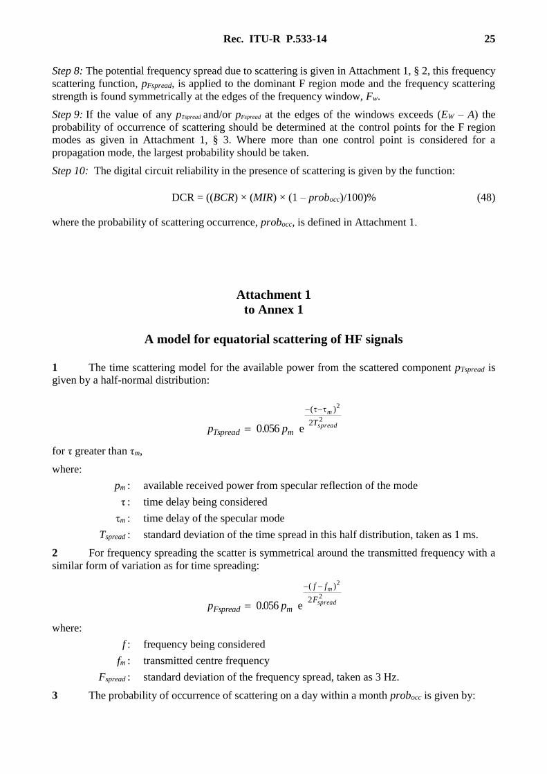
1 The time scattering model for the available power from the scattered component pTspread is

given by a half-normal distribution:

2

2

2

)(

e0560 spread

m

TmTspread p.p

for τ greater than τm,

where:

pm : available received power from specular reflection of the mode

τ : time delay being considered

τm : time delay of the specular mode

Tspread : standard deviation of the time spread in this half distribution, taken as 1 ms.

2 For frequency spreading the scatter is symmetrical around the transmitted frequency with a

similar form of variation as for time spreading:

2

2

2

)(

e0560 spread

m

F

ff

mFspread p.p

where:

f : frequency being considered

fm : transmitted centre frequency

Fspread : standard deviation of the frequency spread, taken as 3 Hz.

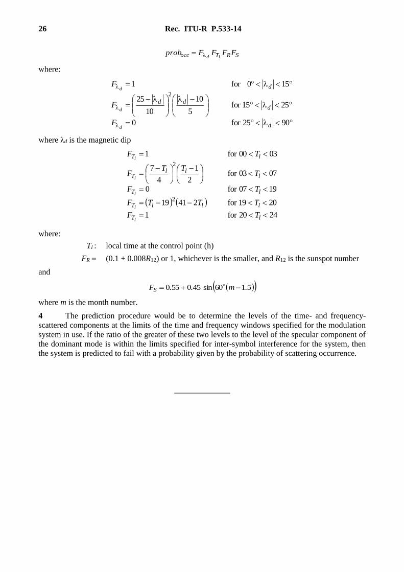
3 The probability of occurrence of scattering on a day within a month probocc is given by:

26 Rec. ITU-R P.533-14

SRTocc FFFFprobld

where:

9025for0

2515for5

10

10

25

150for1

2

d

ddd

d

d

d

d

F

F

F

where λd is the magnetic dip

2420for1

2019for24119

1907for0

0703for2

1

4

7

0300for1

2

2

lT

lllT

lT

lll

T

lT

TF

TTTF

TF

TTT

F

TF

l

l

l

l

l

where:

Tl : local time at the control point (h)

FR (0.1 + 0.008R12) or 1, whichever is the smaller, and R12 is the sunspot number

and

1.560sin0.450.55 mFS

where m is the month number.

4 The prediction procedure would be to determine the levels of the time- and frequency-

scattered components at the limits of the time and frequency windows specified for the modulation

system in use. If the ratio of the greater of these two levels to the level of the specular component of

the dominant mode is within the limits specified for inter-symbol interference for the system, then

the system is predicted to fail with a probability given by the probability of scattering occurrence.