1

Karl W Broman

Biostatistics & Medical InformaticsUniversity of Wisconsin – Madison

http://www.biostat.wisc.edu/~kbroman

Recombination and Linkage

2

The genetic approach

• Start with the phenotype; find genes the influence it.– Allelic differences at the genes result in phenotypic differences.

• Value: Need not know anything in advance.

• Goal– Understanding the disease etiology (e.g., pathways)

– Identify possible drug targets

3

Approaches togene mapping

• Experimental crosses in model organisms

• Linkage analysis in human pedigrees– A few large pedigrees

– Many small families (e.g., sibling pairs)

• Association analysis in human populations– Isolated populations vs. outbred populations

– Candidate genes vs. whole genome

2

4

Linkage vs. association

Advantages• If you find something, it is real

• Power with limited genotyping

• Numerous rare variants okay

Disadvantages• Need families

• Lower power if common variantand lots of genotyping

• Low precision of localization

5

Outline

• Meiosis, recombination, genetic maps

• Parametric linkage analysis

• Nonparametric linkage analysis

• Mapping quantitative trait loci

6

Meiosis

3

7

Genetic distance

• Genetic distance between two markers (in cM) =

Average number of crossovers in the intervalin 100 meiotic products

• “Intensity” of the crossover point process

• Recombination rate varies by– Organism– Sex– Chromosome– Position on chromosome

8

Crossover interference

• Strand choice→ Chromatid interference

• Spacing→ Crossover interference

Positive crossover interference: Crossovers tend not to occur too close together.

9

Recombination fraction

We generally do not observe thelocations of crossovers; rather, weobserve the grandparental originof DNA at a set of geneticmarkers.

Recombination across an intervalindicates an odd number ofcrossovers.

Recombination fraction = Pr(recombination in interval) = Pr(odd no. XOs in interval)

4

10

Map functions

• A map function relates the genetic length of an intervaland the recombination fraction.

r = M(d)

• Map functions are related to crossover interference,but a map function is not sufficient to define the crossoverprocess.

• Haldane map function: no crossover interference

• Kosambi: similar to the level of interference in humans

• Carter-Falconer: similar to the level of interference in mice

11

Linkage in largehuman pedigrees

12

Before you do anything…

• Verify relationships between individuals

• Identify and resolve genotyping errors

• Verify marker order, if possible

• Look for apparent tight double crossovers,indicative of genotyping errors

5

13

Parametric linkage analysis• Assume a specific genetic model.

For example:– One disease gene with 2 alleles– Dominant, fully penetrant– Disease allele frequency known to be 1%.

• Single-point analysis (aka two-point)– Consider one marker (and the putative disease gene)– θ = recombination fraction between marker and disease gene– Test H0: θ = 1/2 vs. Ha: θ < 1/2

• Multipoint analysis– Consider multiple markers on a chromosome– θ = location of disease gene on chromosome– Test gene unlinked (θ = ∞) vs. θ = particular position

14

Phase known

15

Likelihood function

6

16

Phase unknown

17

Likelihood function

18

Missing data

The likelihood now involves a sum over possible parentalgenotypes, and we need:– Marker allele frequencies

– Further assumptions: Hardy-Weinberg and linkage equilibrium

7

19

More generally

• Simple diallelic disease gene– Alleles d and + with frequencies p and 1-p– Penetrances f0, f1, f2, with fi = Pr(affected | i d alleles)

• Possible extensions:– Penetrances vary depending on parental origin of disease allele

f1 → f1m, f1p

– Penetrances vary between people (according to sex, age, or otherknown covariates)

– Multiple disease genes

• We assume that the penetrances and disease allelefrequencies are known

20

Likelihood calculations

• Defineg = complete ordered (aka phase-known) genotypes for all individuals

in a familyx = observed “phenotype” data (including phenotypes and phase-

unknown genotypes, possibly with missing data)

• For example:

• Goal:

21

The parts

• Prior = Pop(gi) Founding genotype probabilities

• Penetrance = Pen(xi | gi) Phenotype given genotype

• Transmission Transmission parent → child

= Tran(gi | gm(i), gf(i))

Note: If gi = (ui, vi), where ui = haplotype from mom and vi = that from dad

Then Tran(gi | gm(i), gf(i)) = Tran(ui | gm(i)) Tran(vi | gf(i))

8

22

Examples

23

The likelihood

Phenotypes conditionallyindependent given genotypes

F = set of “founding” individuals

24

That’s a mighty big sum!

• With a marker having k alleles and a diallelic diseasegene, we have a sum with (2k)2n terms.

• Solution:– Take advantage of conditional independence to factor the sum

– Elston-Stewart algorithm: Use conditional independence inpedigree

• Good for large pedigrees, but blows up with many loci

– Lander-Green algorithm: Use conditional independence alongchromosome (assuming no crossover interference)

• Good for many loci, but blows up in large pedigrees

9

25

Ascertainment

• We generally select families according to their phenotypes. (Forexample, we may require at least two affected individuals.)

• How does this affect linkage?

If the genetic model is known, it doesn’t: we can condition on theobserved phenotypes.

26

Model misspecification

• To do parametric linkage analysis, we need to specify:– Penetrances– Disease allele frequency– Marker allele frequencies– Marker order and genetic map (in multipoint analysis)

• Question: Effect of misspecification of these things on:– False positive rate– Power to detect a gene– Estimate of θ (in single-point analysis)

27

Model misspecification

• Misspecification of disease gene parameters (f’s, p) haslittle effect on the false positive rate.

• Misspecification of marker allele frequencies can lead to agreatly increased false positive rate.– Complete genotype data: marker allele freq don’t matter

– Incomplete data on the founders: misspecified marker allelefrequencies can really screw things up

– BAD: using equally likely allele frequencies

– BETTER: estimate the allele frequencies with the available data(perhaps even ignoring the relationships between individuals)

10

28

Model misspecification

• In single-point linkage, the LOD score is relatively robustto misspecification of:– Phenocopy rate– Effect size– Disease allele frequency

However, the estimate of θ is generally too large.

• This is less true for multipoint linkage (i.e., multipointlinkage is not robust).

• Misspecification of the degree of dominance leads togreatly reduced power.

29

Other things

• Phenotype misclassification (equivalent to misspecifying penetrances)• Pedigree and genotyping errors• Locus heterogeneity• Multiple genes• Map distances (in multipoint analysis), especially if the distances are

too small.

All lead to:– Estimate of θ too large– Decreased power– Not much change in the false positive rate

Multiple genes generally not too bad as long as you correctlyspecify the marginal penetrances.

30

Software

• Lipedftp://linkage.rockefeller.edu/software/liped

• Fastlinkhttp://www.ncbi.nlm.nih.gov/CBBresearch/Schaffer/fastlink.html

• Genehunterhttp://www.fhcrc.org/labs/kruglyak/Downloads/index.html

• AllegroEmail allegro@decode.is

• Merlinhttp://www.sph.umich.edu/csg/abecasis/Merlin

11

31

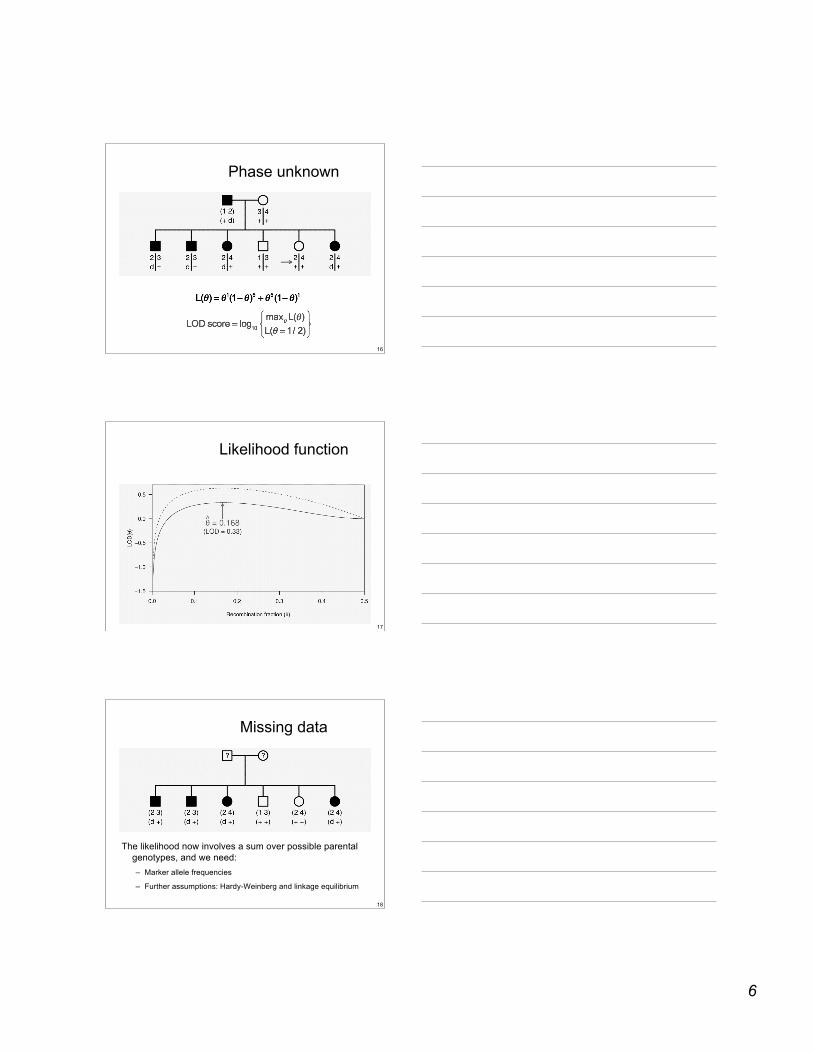
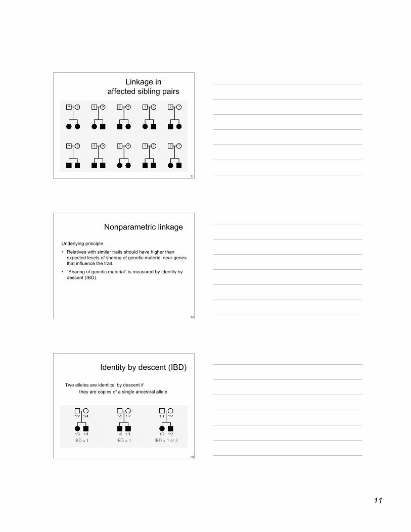
Linkage inaffected sibling pairs

32

Nonparametric linkage

Underlying principle

• Relatives with similar traits should have higher thanexpected levels of sharing of genetic material near genesthat influence the trait.

• “Sharing of genetic material” is measured by identity bydescent (IBD).

33

Identity by descent (IBD)

Two alleles are identical by descent ifthey are copies of a single ancestral allele

12

34

IBD in sibpairs

• Two non-inbred individuals share 0, 1, or 2 alleles IBD atany given locus.

• A priori, sib pairs are IBD=0,1,2 with probability1/4, 1/2, 1/4, respectively.

• Affected sibling pairs, in the region of a diseasesusceptibility gene, will tend to share more alleles IBD.

35

Example

• Single diallelic gene with disease allele frequency = 10%

• Penetrances f0 = 1%, f1 = 10%, f2 = 50%

• Consider position rec. frac. = 5% away from gene

0.760.1280.5030.3681 affected, 1 not

1.000.2520.5000.248Neither affected

1.380.4420.4950.063Both affected

Ave. IBD210Type of sibpair

IBD probabilities

36

Complete data case

Set-up• n affected sibling pairs

• IBD at particular position known exactly

• ni = no. sibpairs sharing i alleles IBD

• Compare (n0, n1, n2) to (n/4, n/2, n/4)

• Example: 100 sibpairs(n0, n1, n2) = (15, 38, 47)

13

37

Affected sibpair tests

• Mean test

Let S = n1 + 2 n2.

Under H0: π = (1/4, 1/2, 1/4),

E(S | H0) = n var(S | H0) = n/2

Example: S = 132Z = 4.53LOD = 4.45

38

Affected sibpair tests

• χ2 test

Let π0 = (1/4, 1/2, 1/4)

Example: X2 = 26.2LOD = X2/(2 ln10) = 5.70

39

Incomplete data

• We seldom know the alleles shared IBD for a sib pair exactly.

• We can calculate, for sib pair i,

pij = Pr(sib pair i has IBD = j | marker data)

• For the means test, we use in place of nj

• Problem: the deminator in the means test,is correct for perfect IBD information, but is too small in the case ofincomplete data

• Most software uses this perfect data approximation, which can makethe test conservative (too low power).

• Alternatives: Computer simulation; likelihood methods (e.g., Kong &Cox AJHG 61:1179-88, 1997)

14

40

Larger families

Inheritance vector, v Two elements for each subject = 0/1, indicating grandparental origin of DNA

41

Score function

• S(v) = number measuring the allele sharing amongaffected relatives

• Examples:– Spairs(v) = sum (over pairs of affected relatives) of no. alleles IBD

– Sall(v) = a bit complicated; gives greater weight to the case thatmany affected individuals share the same allele

– Sall is better for dominance or additivity; Spairs is better forrecessiveness

• Normalized score, Z(v) = {S(v) – µ} / σ– µ = E{ S(v) | no linkage }– σ = SD{ S(v) | no linkage }

42

Combining families

• Calculate the normalized score for each familyZi = {Si – µi} / σi

• Combine families using weights wi ≥ 0

• Choices of weights– wi = 1 for all families– wi = no. sibpairs– wi = σi (i.e., combine the Zi’s and then standardize)

• Incomplete data– In place of Si, use

where p(v) = Pr( inheritance vector v | marker data)

15

43

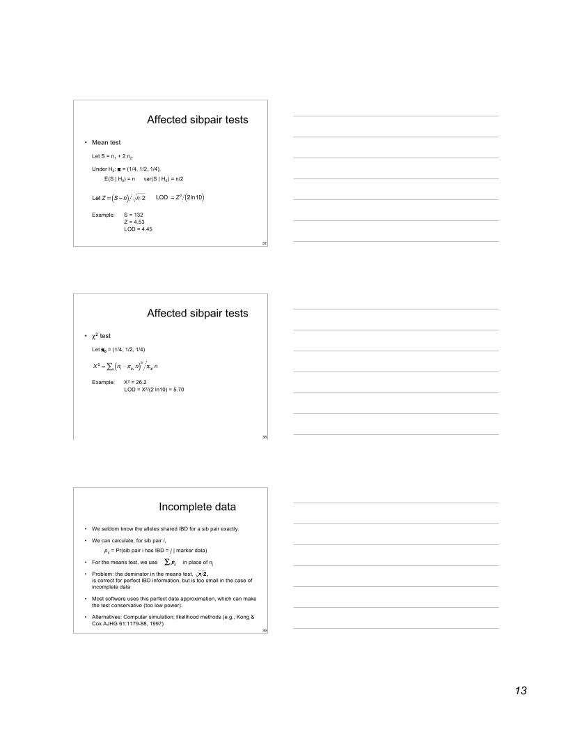
Software

• Genehunterhttp://www.fhcrc.org/labs/kruglyak/Downloads/index.html

• AllegroEmail allegro@decode.is

• Merlinhttp://www.sph.umich.edu/csg/abecasis/Merlin

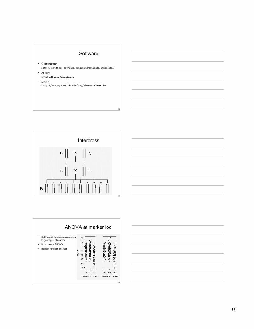
44

Intercross

45

ANOVA at marker loci

• Split mice into groups accordingto genotype at marker

• Do a t-test / ANOVA

• Repeat for each marker

16

46

Humans vs Mice

• More than two alleles

• Don’t know QTL genotypes

• Unknown phase

• Parents may be homozygous

• Markers not fully informative

• Varying environment

47

Diallelic QTL

48

IBD = 2

17

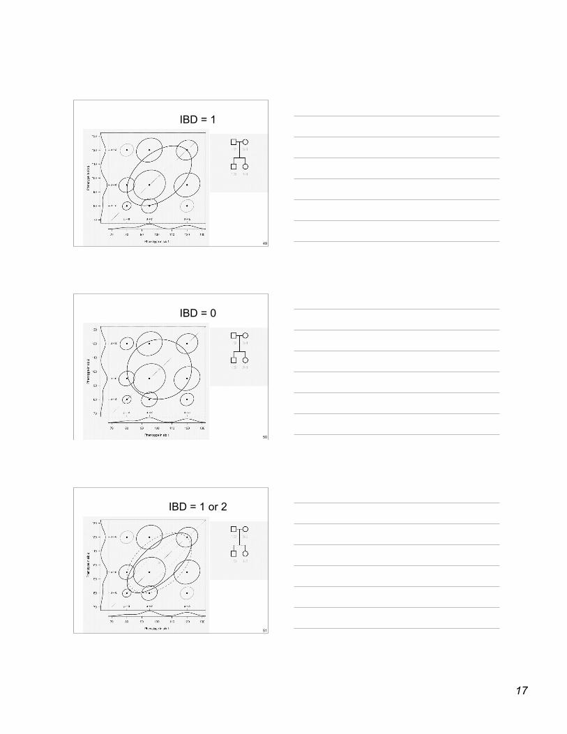
49

IBD = 1

50

IBD = 0

51

IBD = 1 or 2

18

52

Haseman-Elston regression

For sibling pairs with phenotypes (yi1, yi2),– Regression the squared difference (yi1 – yi2)2 on IBD status

– If IBD status is not known precisely, regress on the expected IBDstatus, given the available marker data

There are a growing number of alternatives to this.

53

Challenges

• Non-normality

• Genetic heterogeneity

• Environmental covariates

• Multiple QTL

• Multiple phenotypes

• Complex ascertainment

• Precision of mapping

54

Summary• Experimental crosses in model organisms

+ Cheap, fast, powerful, can do direct experiments– The “model” may have little to do with the human disease

• Linkage in a few large human pedigrees+ Powerful, studying humans directly– Families not easy to identify, phenotype may be unusual, and

mapping resolution is low

• Linkage in many small human families+ Families easier to identify, see the more common genes– Lower power than large pedigrees, still low resolution mapping

• Association analysis+ Easy to gather cases and controls, great power (with sufficient

markers), very high resolution mapping– Need to type an extremely large number of markers (or very good

candidates), hard to establish causation

19

55

References

• Lander ES, Schork NJ (1994) Genetic dissection of complex traits. Science265:2037–2048

• Sham P (1998) Statistics in human genetics. Arnold, London

• Lange K (2002) Mathematical and statistical methods for genetic analysis, 2ndedition. Springer, New York

• Kong A, Cox NJ (1997) Allele-sharing models: LOD scores and accuratelinkage tests. Am J Hum Gene 61:1179–1188

• McPeek MS (1999) Optimal allele-sharing statistics for genetic mapping usingaffected relatives. Genetic Epidemiology 16:225–249

• Feingold E (2001) Methods for linkage analysis of quantitative trait loci inhumans. Theor Popul Biol 60:167–180

• Feingold E (2002) Regression-based quantitative-trait-locus mapping in the21st century. Am J Hum Genet 71:217–222