Adv. Appl. Prob. 31, 1002–1026 (1999)Printed in Northern Ireland

Applied Probability Trust 1999

RECENT COMMON ANCESTORS OF ALL PRESENT-DAYINDIVIDUALS

JOSEPH T. CHANG,∗ Yale University

Abstract

Previous study of the time to a common ancestor of all present-day individuals hasfocused on models in which each individual has just one parent in the previousgeneration. For example, ‘mitochondrial Eve’ is the most recent common ancestor(MRCA) when ancestry is defined only through maternal lines. In the standard Wright–Fisher model with population size n, the expected number of generations to the MRCAis about 2n, and the standard deviation of this time is also of order n. Here we study atwo-parent analog of the Wright–Fisher model that defines ancestry using both parents.In this model, if the population size n is large, the number of generations, T n, back toa MRCA has a distribution that is concentrated around lg n (where lg denotes base-2logarithm), in the sense that the ratio Tn/(lg n) converges in probability to 1 as n→ ∞.Also, continuing to trace back further into the past, at about 1.77 lg n generations beforethe present, all partial ancestry of the current population ends, in the following sense:with high probability for large n, in each generation at least 1.77 lg n generations beforethe present, all individuals who have any descendants among the present-day individualsare actually ancestors of all present-day individuals.

Keywords: Coalescent; Wright–Fisher model; Galton–Watson process; genealogicalmodels; population genetics

AMS 1991 Subject Classification: Primary 92D25Secondary 60J85

1. Introduction

Starting with the set of all of us present-day humans, imagine tracing back in time throughour mothers, our mothers’ mothers, and so on. This is the maternal family tree of mankind,and we are at its leaves. Recent research has suggested that the woman at the root of this treelived roughly 100 000 or 200 000 years ago, perhaps in Africa (Cann et al. (1987); Vigilantet al. (1991)). This woman has been dubbed ‘mitochondrial Eve’, since all present-day humanmitochondrial DNA descended from hers. Mitochondrial Eve was undoubtedly not the onlywoman alive at her time, so the name ‘Eve’ is misleading, as has been pointed out by anumber of authors; see, for example, Ayala (1995). However, this misunderstanding aside,questions of the origins of mankind and the nature of our relationships to each other are stillof keen interest, and the research on mitochondrial Eve has received a great deal of publicity,generating headlines in the popular press as well as in scientific publications. Svante Paabo(1995) explains:

Received 9 October 1997; revision received 19 June 1998.∗ Postal address: Statistics Department, Yale University, Box 208290, New Haven, CT 06520, USA.Email address: joseph.chang@yale.edu

1002

Recent common ancestors 1003

. . . the recent date of our mitochondrial ancestor is in a sense the really controver-sial conclusion from these studies. Everyone agrees that we trace our ancestry toHomo erectus, who emerged in Africa and from there colonized most of Eurasiaabout a million years ago or even earlier. What the mitochondrial data seem toshow, however, is that we have a much more recent ancestor, one who lived some100 000 or 200 000 years ago.

What captures the imagination is not the particular choice to trace back through the maternalline, but rather it is the idea that all of present-day humanity may have a common ancestor wholived as little as 100 000 years ago, a time that seems to many to be surprisingly recent. If weretain this idea while removing the restriction to the maternal line, the question becomes:How far back in time do we need to trace the full genealogy of mankind in order to find anyindividual who is a common ancestor of all present-day individuals? In this paper we addressthis sort of question in a simple mathematical model.

The coalescent model of Kingman (1982a) forms the basis of many of the calculations,formal and informal, used in recent treatments of questions about mitochondrial Eve andrelated topics. The coalescent is a large-population limit of a number of the fundamental mod-els of population genetics, including the Wright–Fisher process. These models are haploid,with each individual in a given generation having a single parent in the previous generation.The Wright–Fisher model assumes ‘random mating’, in the sense that the parent of a givenindividual is equally likely to be any of the individuals in the previous generation. The standardmodel also postulates a constant population size, which may be an ‘effective population size’when modeling more general situations. A number of important properties of the coalescentmodel are used in applications. For example, the model implies a relationship between coales-cence times and population size: the expected coalescence time (measured in generations) ofa large sample is about twice the population size. Hudson (1990) gives a survey of the theoryand applications of the coalescent.

Here we study a natural two-parent analog of the Wright–Fisher process. (This process waspreviously considered by Kammerle (1991) and Mohle (1994); see the end of this section fora discussion of related work.) We assume the population size is constant at n. Generationsare discrete and non-overlapping. The genealogy is formed by this random process: in eachgeneration, each individual chooses two parents at random from the previous generation. Thechoices are made just as in the standard Wright–Fisher model—randomly and equally likelyover the n possibilities—the only difference being that here each individual chooses twiceinstead of once. All choices are made independently. Thus, for example, it is possible thatwhen an individual chooses his two parents, he chooses the same individual twice, so that infact he ends up with just one parent; this happens with probability 1/n.

This model is designed only as a simple starting point for thought; of course it is not meantto be particularly realistic. Still, one might worry that this simple model ignores considerationsof sex and allows impossible genealogies. If this seems bothersome, an alternative interpreta-tion of the same process is that each ‘individual’ is actually a couple, and that the populationconsists of n monogamous couples. Then the random choices cause no contradictions: thehusband and wife each were born to a couple from the previous generation. They could evencome from the same couple in the previous generation.

Our interest here is in finding individuals who are common ancestors of all present-dayindividuals. For convenience, we use the abbreviation ‘CA’ to refer to a common ancestor ofall present-day individuals, and ‘MRCA’ stands for ‘most recent common ancestor.’

1004 J. T. CHANG

It turns out that mixing occurs extremely rapidly in the two-parent model, so that CAs maybe found within a number of generations that depends logarithmically on the population size.In particular, our first main result says that the number of generations back to an MRCA isabout lg n, where lg denotes logarithm to base 2.

Theorem 1. Let Tn denote the number of generations, counting back in time from the present,to an MRCA of all present-day individuals, in a population of size n. Then

Tnlg n

P→ 1 as n→ ∞.

This contrasts dramatically with the one-parent situation. For example if n is 1 million, thenthe one-parent MRCA (‘Eve’) is expected to occur about 2 million generations ago, whereasa two-parent MRCA occurs with high probability within the last 20 generations or so. Also,the variability in the one-parent situation is such that the actual time to the MRCA may easilybe as small as half the expected time or as large as double the expected time, say, even inarbitrarily large populations. In contrast, the time to an MRCA for the two-parent model ismuch less variable. For example, if the population is large enough, it is very unlikely that arandom realization of the two-parent MRCA time will differ from lg n by even one percent.

This paper also addresses a second related question. Imagine tracing back through thetwo-parent genealogy. According to Theorem 1, after about lg n generations, we will reachthe most recent generation that contains a CA. That generation might contain just one CA,or it might contain more than one. In any case, if we continue tracing back further throughsuccessive generations, then the title ‘CA’ becomes much less of a prestigious distinction. Forexample, both parents of a CA will be CAs, and all grandparents of a CA will be CAs, and soon. Eventually, in a given generation, many (and in fact most) of the individuals will be CAs.At some point we reach a generation in which some individuals are CAs (having all present-day individuals as descendants) and some are ‘extinct’ (having no present-day individuals asdescendants), but no individual is intermediate (having some but not all present-day individualsas descendants). That is, at this point, everyone who is not extinct is a CA. This conditionpersists forever as we trace back in time: every individual is a CA or extinct. The next resultshows that this condition is reached very rapidly in the model studied here.

Theorem 2. Let Un denote the number of generations, counting back in time before thepresent, to a generation in which each individual is either a CA of all present-day individualsor an ancestor of no present-day individual. Let γ denote the smaller of the two numberssatisfying the equation γ e−γ = 2 e−2, and let ζ = −1/(lg γ ) ≈ 0.7698. Then

Un

(1 + ζ ) lg nP→ 1 as n→ ∞.

Thus, within about 1.77 lg n generations, a tiny amount of time in comparison with theorder n time required to get a one-parent CA, everyone in the population is either a CA of allpresent-day individuals or extinct.

Figure 1 shows a small example to illustrate the definitions and statements. The populationsize is 5. At the bottom of the figure is generation 0, the present. Going up in the graphcorresponds to going back in time, so that the top row is generation −5. For each individualI in each previous generation, we calculate the set of present-day individuals (individualsin generation 0) that are descendants of I . For example, the set of present-day descendantsof individual #1 in generation −1 is {3, 5}. The calculations propagate backward in time

Recent common ancestors 1005

1 32 4 5

{3,5}{2,3} {4} {5} {1,2,4}

{4,5}{1,2,3,4} {2,3}

S 0/

SS {4,5} {1,2,3,4}0/

{4,5} S 0/ SS

SS

S0/ 0/

Figure 1: An example illustrating the model. Here the fourth individual in generation −2 is a CA. Bygeneration −5, all individuals are CAs or extinct: individuals 1,4, and 5 are CAs, and individuals 2 and

3 are extinct.

according to the rule: the set of descendants of an individual I is the union of the sets ofdescendants of the children of I . For example, the set of present-day descendants of individual#4 in generation −2 is the union {3, 5} ∪ {5} ∪ {1, 2, 4}, which is the whole population S.Thus, individual #4 in generation −2 is a CA of the set S of all present-day individuals.Continuing backward in time, at generation −5 we reach the stage where each individualhas as descendants either the whole population S or the empty set ∅. That is, each individualin generation −5 is either a CA or extinct, having as descendants either everybody or nobodyfrom the set of present-day individuals, and all generations prior to generation −5 also havethis property. In the example shown, T5 = 2 and U5 = 5.

What is the significance of these results? An application to the world population of humanswould be an obvious misuse. For example, we would not claim that a common ancestor ofevery present-day human may be found within the last lg n generations. Even if we took nto be 5 billion, this would imply a CA just about 32 generations ago—perhaps 500 years orso. An important source of the inapplicability of the model to this situation is the obviousnon-random nature of mating in the history of mankind. For example, parents are much morelikely to live within a few miles of their children than a thousand miles away or halfwayaround the world. So the model studied here is too simple to be directly applicable to theevolution of mankind as a whole. In such complicated situations, the results sound a noteof caution: if the logarithmic time to CAs seems patently implausible, then at least one ofthe assumptions of the model, such as the random mating assumption, must be causing agreat deal of trouble. On the other hand, it would be interesting to know whether there aresimpler real-life situations in which the assumptions of the model do apply reasonably welland the theorems provide reasonably accurate quantitative descriptions. Perhaps a relativelyhomogeneous population lacking discernible structures (geographic or otherwise) that interactstrongly with reproduction would be a promising candidate.

1006 J. T. CHANG

The random time analysed in Theorem 2 seems of natural interest in this process and mayalso be pertinent to certain questions about ‘species trees’ or ‘population trees’ (as opposed to‘gene trees’). In many contexts the species tree is considered to be the real object of interest,and we use genetic data and gene trees to attempt to learn about the species tree. For example,for humans, chimpanzees, and gorillas, is the ‘true species tree’ (HC)G, (HG)C, or (CG)H?Roughly, the conceptual framework of this question is as follows. There were two ‘speciationevents’ that split a single species ancestral to humans, chimpanzees, and gorillas into the threeseparate modern species. The tree (HC)G, for example, says that the first such split separatedthe subpopulation that eventually became modern gorillas from the remainder, which latersplit to become modern humans and chimpanzees. Unfortunately, more precise definitions ofthe concept of species tree that remain useful in difficult or unclear cases seem hard to comeby. One might adopt the viewpoint that the proper starting point for a definition of ‘speciestree’ is the full two-parent genealogy of all present-day individuals. Given such a definition,if we knew all details of this genealogy, then we could read off an answer to the H , C, andG question (the answer might be ‘none of the 3 choices above’—that is, the species tree isnot well defined or at least not bifurcating). One interpretation of the time Un is as follows.Suppose we imagine a case where evolution really proceeded according to a neat successionof ‘speciation events’. Under a certain reasonable definition of a species tree, if the timesbetween those speciation events exceed Un, then the species tree is guaranteed to be welldefined and coincide with the history of speciation events. This idea will be discussed morefully elsewhere.

A caveat to forestall potential misunderstanding: this paper is not about genetics. That is, itis not about who gets what genes; it is about something more primitive, namely, the ancestor–descendant relationship. One-parent models are appropriate in tracing the history of a sampleof nonrecombining genes or small bits of DNA; a single nucleotide descends from a singlenucleotide from either the mother or father, but not both. Here we are considering ancestry inthe more common, demographic sense of the word, as applied to people, for example, ratherthan genes.

Previous genetics research that is somewhat related, although still very different from thepresent study, considers models incorporating recombination. This type of model has beeninvestigated in a number of papers, including those of Hudson (1983) and Griffiths andMarjoram (1997). The history of a sample of DNA sequences may be described by a collectionof genealogies, with each nucleotide position in the DNA having its own one-parent genealogy.The genealogies for two positions that experience no recombination between them will becongruent, with the paths of the two genealogies going back through the same individuals,whereas a recombination between two positions causes the genealogies of those positions todiffer. Each of the genealogies in the collection will have its own MRCA (the nucleotide atits root), which may occur in different individuals. Each of these individuals will be a CAin the sense considered in this paper, but the most recent of these individuals is generallynot an MRCA in our sense. Our MRCA is more recent, since the paths from ancestorsto descendants consist of all potential paths for genes to be transmitted, and may includepaths that did not happen to be taken by any genes. No previous results about these geneticmodels have been similar to the results here, for example, in getting times of order log n.This is not surprising, since the asymptotics would require an assumption that the sequencelengths and the number of recombinations tend to infinity. This is another manifestationof the statement that the questions we are investigating here are not fundamentally geneticsquestions.

Recent common ancestors 1007

There is some previous work on the process we study here and related processes. Twopapers of Kammerle (1989, 1991) introduce a general class of two-parent (called ‘bisexual’in those papers) versions of the Wright–Fisher and other processes. These papers focus ontwo main questions. First, they analyse the probability of extinction of a set of individualsin the present generation, that is, the probability that the set of individuals eventually hasno descendants in some future generation. Second, in a two-parent version of the Moranmodel, they study the number Rn(t) of individuals t generations ago who have at least onedescendant in the present generation. Kammerle (1989) finds that the Markov chain {Rn(t) :t = 0, 1, . . . }, suitably normalized and suitably initialized (with the initialization essentiallyrequiring that the chain is started in steady state), converges weakly as n → ∞ to a discrete-time Ornstein–Uhlenbeck process.

Mohle (1994) both generalizes and refines the results of Kammerle. In particular, Mohleprovides a detailed analysis of the extinction probabilities in a two-parentWright–Fisher modelthat approximates the probabilities up to o(1/n). He also establishes weak convergence in ageneral class of two-parent models, including an Ornstein–Uhlenbeck limit for the two-parentWright–Fisher process. Mohle also has a number of other papers in press, including one thatrelaxes the assumption of constant population size.

These previous results are complementary to the results in this paper. The previous papersconsidered individuals who have at least one descendant in a given future generation. Here weconsider CAs, who have as descendants all members of the future generation. The previousresults about the process {Rn(t)} apply to large t , that is, to the behavior of the process manygenerations before the present, with the process in steady state. Here we focus on the behaviorof a related process at small (i.e. recent) times, starting far away from steady state. We showthat at about t = 1.77 lg n generations before the present, with high probability the Rn(t)individuals who have at least one present-day descendant are all in fact CAs.

2. Simulations

Table 1 presents a small simulation study consisting of 25 trials each for n = 500, n = 1000,n = 2000, and n = 4000. Two numbers are reported for each trial: Tn, the number ofgenerations back to an MRCA, and Un, the generation at which every individual is either aCA or extinct.

In these simulations the distribution of the time back to an MRCA is indeed quite concen-trated around the value lg n, which is nearly 9 for n = 500, nearly 10 for n = 1000, and soon. Thus, the simulation results show that the asymptotic (n→ ∞) statement of Theorem 1 is‘not so asymptotic’, in that it describes the situation well even for rather small values of n. Thebehavior predicted by Theorem 2 is also reflected reasonably well in the simulations, althoughone might have guessed a numerical constant closer to 2 rather than 1.77 from this small study.

3. Proofs

3.1. General ideas and tools

We start with the observation that although Theorems 1 and 2 are phrased in terms ofcounting generations back in time from the present until some condition obtains, these resultsmay be proved by counting forward in time from a fixed generation. For example, the event{Tn ≤ m} requires that a CA of all individuals in generation 0 may be found among generations−1,−2, . . . ,−m. This is equivalent to requiring that if we start with generation −m and traceforward in time, then some individual in generation −m becomes a CA of all individuals insome generation t ∈ {−m+ 1,−m+ 2, . . . , 0}.

1008 J. T. CHANG

Table 1: A small simulation study. For each of four population sizes n, the two times Tn and Un arereported for 25 trials.

n = 500 n = 1000 n = 2000 n = 4000

1 10 18 11 19 12 24 13 242 9 18 11 21 12 22 13 233 10 21 10 20 11 23 12 244 9 18 11 20 12 22 13 245 10 19 10 20 12 21 13 246 9 19 11 31 12 23 13 247 10 19 11 20 12 21 13 248 10 21 10 23 12 27 13 249 9 19 11 20 11 24 13 24

10 9 17 11 20 12 24 13 3111 9 19 10 21 12 26 13 2312 9 18 11 21 11 22 13 2313 9 19 11 21 12 21 13 2514 9 20 11 20 12 25 13 2215 9 19 10 20 11 24 13 2416 10 21 10 21 11 23 13 2317 9 19 11 19 12 24 13 2318 9 17 10 26 12 22 13 2419 9 19 11 21 11 23 13 2520 10 18 10 21 12 22 13 2521 9 19 11 19 12 22 12 2522 10 19 11 26 12 22 13 2623 9 19 10 20 12 24 13 2724 10 17 11 21 12 22 13 2625 10 19 11 23 12 23 13 25

So we will count generations forward in time, and for convenience let us renumber genera-tions so that the initial generation is ‘generation 0’. The population at generation t ≥ 0 consistsof n individuals denoted by It,1, It,2, . . . , It,n. We can picture It,1, It,2, . . . , It,n as dots in anarray as in Figure 1, with It,j being the j th dot in row t . The association of a number j toindividual It,j is an arbitrary labeling of the individuals within generation t . Assigned onlyas a means of referring to individuals, the labels have no significance in the model, whichdoes not order the individuals within a generation. Let µt,1, νt,1, µt,2, νt,2, . . . , µt,n, νt,n beindependent and uniformly distributed on the set {1, . . . , n}. We interpret µt,j and νt,j aslabels of the parents of individual It,j ; that is, the parents of It,j are It−1,µt,j and It−1,νt,j .Defining a sequence of random sets Gi0,G

i1, . . . recursively by Gi0 = {i} and

Git = {j ≤ n : µt,j ∈ Git−1 or νt,j ∈ Git−1},

Git is the set of labels of the descendants of I0,i in generation t . Let Git denote the cardinalityof Git . The conditional probability that individual It+1,j has at least one parent among the Gitmembers of Git is

P({µt+1,j ∈ Git } ∪ {νt+1,j ∈ Git } | Git ) = (Git /n)+ (Git /n)− (Git /n)(Git /n).

Recent common ancestors 1009

The process {Git : t = 0, 1, . . . } is a Markov chain with transition probabilities

(Git+1 | Git ) ∼ Bin

(n,

2Gitn

−(Git

n

)2), (1)

where Bin(n, p) denotes the binomial distribution for the number of successes in n indepen-dent trials each having success probability p.

Throughout the proof, {Gt } will denote a Markov chain with transition probabilities as in(1), although in different parts of the proof we will consider different possible initial valuesG0. For example, taking G0 = 1 corresponds to following the descendants of a particularindividual in generation 0. In the early stages of the process, while Gt remains small relativeto n, in view of (1) the conditional distribution ofGt+1 givenGt is nearly Poisson(2Gt), that is,the Poisson distribution with mean 2Gt . In other words, while {Gt } remains small, it evolvesnearly as a Galton–Watson branching process {Yt } with offspring distribution Poisson(2).Kammerle (1991) gave a formal statement of a result of this nature. A special case of hisresult says that for fixed u, the joint distribution of (G0,G1, . . . ,Gu) converges to that of(Y0, Y1, . . . , Yu) as n → ∞. For our purposes, we will use the following result that allows usto approximate probabilities for the G process by those for the Y process up to a higher orderof accuracy and over longer intervals of time that may have random lengths.

Lemma 3. Let Y0, Y1, . . . denote a Galton–Watson branching process with offspring dis-tribution Poisson(2). Suppose that Y0 = G0 = 1. Define τYb = inf{t : Yt ≥ b} andτY0b = inf{t : Yt = 0 or Yt ≥ b}, with corresponding definitions for τGb and τG0b. As n→ ∞, ifm and b satisfy mb2 = o(n), then

P{τGb > m} = P{τYb > m}(1 + o(1)) (2)

andP{τG0b > m} = P{τY0b > m}(1 + o(1)). (3)

Proof.A straightforward calculation bounds the likelihood ratio

L(y | x) : = P{Gt+1 = y | Gt = x}P{Yt+1 = y | Yt = x}

= P{Bin(n, (2x/n)− (x2/n2)) = y}P{Poisson(2x) = y} ≤ e2x(1 − (2x/n)+ (x2/n2))n−y,

so that

logL(y | x) ≤ 2x + (n− y)(

−2x

n+ x2

n2

)≤ (x2 + 2xy)/n.

This holds whenever the denominator P{Yt+1 = y | Yt = x} is positive, that is, for all x > 0and y ≥ 0, and also for x = y = 0. Thus, for all such pairs of x and y satisfying x < b andy < b, we have

logL(y | x) ≤ 3b2/n.

A similar calculation gives the lower bound

logL(y | x) ≥ −5b2/(2n)[1 +O(b/n)],

1010 J. T. CHANG

so that logL(y | x) ≥ −3b2/n for sufficiently large n. So if x1, . . . , xm are all less than b,then

P{G1 = x1, . . . ,Gm = xm} = P{G1 = x1 | G0 = 1} · · · P{Gm = xm | Gm−1 = xm−1}= P{Y1 = x1, . . . , Ym = xm}L(x1 | 1) · · ·L(xm | xm−1)

≤ P{Y1 = x1, . . . , Ym = xm} e3mb2/n

andP{G1 = x1, . . . ,Gm = xm} ≥ P{Y1 = x1, . . . , Ym = xm} e−3mb2/n.

Thus,

P{τGb > m} =∑

0≤x1<b· · ·

∑0≤xm<b

P{G1 = x1, . . . ,Gm = xm}

≤∑

0≤x1<b· · ·

∑0≤xm<b

P{Y1 = x1, . . . , Ym = xm} e3mb2/n

= P{τYb > m} e3mb2/n (4)

and, similarly, P{τGb > m} ≥ P{τYb > m}e−3mb2/n, so that, by the assumption that mb2 =o(n), we obtain P{τGb > m} = P{τYb > m}(1 + o(1)). This proves (2). The proof of (3)uses the same reasoning, with the summations in (4) ranging over 0 < xt < b rather than0 ≤ xt < b.

The previous result will be useful because the Poisson Galton–Watson process is simpleand well understood. The next lemma records a few well known items for future reference.

Lemma 4. Let Y0, Y1, . . . denote a Galton–Watson process with offspring distributionPoisson(2). Define the moment generating function ψ(z) = E(zY1) = e−2+2z. The extinctionprobability ρ = P{Yt = 0 for some t} ≈ 0.20319 is the smaller of the two solutions ofψ(ρ) = ρ, and ρ = γ /2, where γ is as defined in Theorem 2. The t-fold compositionψt = ψ ◦ · · · ◦ ψ satisfies ψt(z) ↑ ρ for all 0 ≤ z ≤ ρ.The relation ρ = γ /2 is confirmed by comparing the definitions of ρ and γ . Despite the simplerelationship, we will keep the two different letters in our notation for conceptual clarity.

Defining gt = Gt/n, we have

E(gt+1 | gt ) = 2gt − g2t = gt (2 − gt ). (5)

That is, if the fraction of descendants of a given individual is currently gt , it is expected tomultiply by a factor of 2 − gt in the next generation. For example, in the early stages of theprocess when the fraction gt is small, it nearly doubles in expectation in the next generation.For very small gt (of the order 1/n, for example) the random variability is large; for example,the process could easily go extinct. This is when it is most useful to approximate theG processby the Poisson(2) Galton–Watson process.

On the other hand, for larger values of gt , the multiplication factor gt+1/gt , althoughexpected to be somewhat smaller, has much less variability. The deviations of this factorfrom its expected value are bounded probabilistically by large deviations inequalities for thebinomial distribution. We will use the following inequality of Bernstein (1946) as a basic tool.

Recent common ancestors 1011

Lemma 5. (Bernstein’s inequality.) If X ∼ Bin(n, p) and r > 0, then

P{X ≥ np + r} ≤ exp

{ −r22np(1 − p)+ (2/3)r

}. (6)

Since n − X ∼ Bin(n, 1 − p), the right-hand side of (6) is also an upper bound for theprobability P{X ≤ np − r}.3.2. Proof of Theorem 1

Outline. The proof will be divided into several parts. We start from generation 0 and traceforward in time.

Stage 1: By the end of Stage 1, we identify an individual I in generation 0 who has anumber of descendants that is small compared to n, but large enough so that I is unlikely everto become extinct. In particular, we look for a generation t such that some individual I ingeneration 0 has at least lg2(n) descendants in generation t . With probability approaching 1,this happens in time o(lg n), negligible compared with lg n; this is shown by using Lemma 3to approximate our process by a Poisson Galton–Watson process. The rest of the proof willshow that with probability approaching 1, individual I becomes a CA within (1 + ε)(lg n)generations, where ε is an arbitrary positive number.

Stage 2: Let β ∈ (0, 1). Stage 2 follows the descendants of I until reaching a generationcontaining at least nβ descendants. In view of (5), since nβ is a small fraction of n for large n,throughout Stage 2 the number of descendants in a generation is expected to be nearly doublethe number of descendants in the previous generation. And lg2(n) is large enough so that themultiplication factor will be very close to its expected value, with high probability. So Stage 2should not take much more than about lg(nβ) = β lg(n) generations.

Stage 3: This stage brings the count of descendants of I up from nβ to (1/2)n. Sincethe fraction of descendants during Stage 3 stays below 1

2 , the expected multiplication factoris at least 2 − 1

2 = 32 . Again, this multiplication factor is very reliable, so that with high

probability Stage 3 takes no more than about log3/2{(n/2)/(nβ)} generations. We can makethis an arbitrarily small fraction of lg n by choosing β close enough to 1.

Stage 4: Now we switch to looking at the fraction Bt of individuals in a generation whoare not descendants of individual I . This fraction is expected to square each generation. Thiscauses Bt to decrease very quickly. Fixing α ∈ ( 12 , 2

3 ), we show that Stage 4, which takes thefraction Bt from 1

2 down to n−α , takes only order lg lg n time.Stage 5: This completes the process, ending when the B process hits 0, and individual I

has become a CA. We show that this takes just one generation with high probability.Upper bound: Combining the results of Stages 1 through 5 gives the probabilistic upper

bound limn→∞ P{Tn ≤ (1 + ε) lg n} = 1.Lower bound: Here we show that limn→∞ P{Tn ≥ (1 − ε) lg n} = 1. This is done by using

Bernstein’s inequality to prove an assertion of the following form: for positive r and δ, oncethe process of descendants of any given individual reaches a power nr of n, it is very unlikelyto increase by a factor of more than 2 + δ in a generation, whereas it would have to do so inorder to have Tn < (1 − ε) lg n.3.2.1. Stage 1. Here we will show that with high probability, within a number of generationsnegligible compared to lg n, we can find a generation with at least lg2 n individuals who sharea common ancestor. For simplicity we give a crude argument that circumvents the need to

1012 J. T. CHANG

consider any dependence among the processes {Git : t ≥ 0} starting from different individualsI0,i . This could also be done along the lines of the argument in Lemma 19 below, where weneed to confront this dependence.

Lemma 6. Define τb = inf{t : Gt ≥ b}. Assuming that G0 = 1,

lim infn→∞ P{τlg2 n ≤ 3 lg lg n} > 0.

Proof. Let b and m denote lg2 n and �3 lg lg n�, respectively. Let {Yt } be a Galton–Watsonprocess with offspring distribution Poisson(2), and defineMt = Yt2−t . The process {Mt } is anon-negative martingale that converges almost surely to a limitM∞, say, with P{M∞ = 0} =ρ < 1. Note that P{τYb > m} ≤ P{Ym < b} = P{Mm < b2−m}. Therefore, using Fatou’slemma and the assumption that b2−m → 0,

lim sup P{τYb > m} ≤ lim sup P{Mm < b2−m} ≤ P(lim sup{Mm < b2−m})= P{Mm < b2−m infinitely often} ≤ P{M∞ = 0} = ρ < 1.

By Lemma 3, P{τb > m} = P{τYb > m}(1 + o(1)) as n→ ∞. Therefore,

lim sup P{τb > m} ≤ lim sup P{τYb > m} ≤ ρ < 1.

So lim inf P{τb ≤ m} ≥ 1 − ρ > 0.

Proposition 7. LetGit denote the number of descendants in generation t of individual I0,i (theith individual in generation 0), and let G∗

t = max1≤i≤n{Git }. Define τG∗b = inf{t : G∗

t ≥ b}.Then τG

∗lg2 n

= oP(lg n).Proof. We use a geometric trials argument. Let mn = �3 lg lg n�, and choose a sequence

{kn} with kn → ∞ and knmn = o(lg n). Perform a sequence of kn trials as follows. Forthe first trial, start with individual I0,1, and follow his progeny for mn generations. We saythe trial is a success if I0,1 has at least lg2 n descendants in generation mn; by Lemma 6 thishappens with probability at least c, say, where c > 0. If the trial is a failure, start a new trial,following the progeny of individual Imn,1 for mn more generations. And so on. We stop at thefirst success, having found an individual with at least lg2 n descendants. The probability thatthis sequence of trials fails to terminate by generation knmn is at most (1 − c)kn , which tendsto 0.

Thus, with probability tending to 1, there is a κ ∈ {0, . . . , kn−1} such that individual Iκmn,1has at least lg2 n descendants in generation (κ + 1)mn. Let I denote any ancestor of Iκmn,1 ingeneration 0. We will show in the remainder of the proof that for each ε > 0, with probabilitytending to 1 as n→ ∞, individual I becomes a CA within (1 + ε) lg n generations.

3.2.2. Stage 2. The following simple consequence of Bernstein’s inequality will be a conveni-ent tool.

Lemma 8. If δ ≤ 3/4 and Gt ≤ δn/20, then

P{Gt+1 ≤ (2 − δ)Gt | Gt } ≤ exp(−δ2Gt/5).

Recent common ancestors 1013

The next result shows that the probability that Stage 2 takes more than lg n generationsapproaches 0 as n → ∞. In fact, we show that this probability is o(1/n); this will be used inthe proof of Theorem 2.

Proposition 9. Assume that G0 ≥ lg2 n, and let 0 < β < 1. Define T2 = inf{t : Gt ≥ nβ}.Then P{T2 > lg n} = o(1/n) as n→ ∞.

Proof. Take 0 < δ < 3/4 such that lg(2 − δ) > β, and define

b(n) =⌈log2−δ

(nβ

lg2 n

)⌉.

Note that

b(n) ≤ β lg n

lg(2 − δ) ≤ lg n,

at least for n ≥ 3, so that P{T2 > lg n} ≤ P{T2 > b(n)}. We will show that P{T2 > b(n)} =o(1/n).

The inequality T2 > b(n) implies that Gt+1 < (2 − δ)Gt for some 0 ≤ t ≤ b(n)− 1. Thefirst such t must also satisfy Gt ≥ lg2 n. Thus,

P{T2 > b(n)} ≤ P

{ b(n)−1⋃t=0

{Gt+1 < (2 − δ)Gt , Gt ≥ lg2 n, T2 > b(n)}}

≤b(n)−1∑t=0

P{Gt+1 < (2 − δ)Gt , lg2 n ≤ Gt ≤ nβ}.

However, nβ ≤ δn/20 for sufficiently large n. Therefore, on the event {lg2 n ≤ Gt ≤ nβ}, wemay apply Lemma 8 to obtain

P{Gt+1 < (2 − δ)Gt | Gt } ≤ exp

(−δ

2

5lg2 n

)= n−(δ2/5)(lg e)(lg n).

Thus,

P{T2 > b(n)} ≤ b(n)n−(δ2/5)(lg e)(lg n) = o(1/n) as n→ ∞.

3.2.3. Stage 3. This stage starts in a generation in which the number of descendants of I isjust over nβ and ends when the number of descendants in a generation reaches 1

2n. Defininggt = Gt/n, we have E(gt+1 | gt ) = gt (2 − gt ). The idea is that if gt ≤ 1

2 , then in the nextgeneration gt is expected to multiply by a factor of 2 − gt ≥ 3

2 . So with high probability,throughout Stage 3, at each generation the number of descendants will multiply by at least√

2, say, since√

2 < 32 . So to get from nβ to 1

2n, we should need at most log√2(

12 )n

1−β =2[(1 − β) lg n− 1] generations.

Proposition 10. Assume G0 ≥ nβ , and define T3 = inf{t : Gt ≥ ( 12 )n}. Then P{T3 >

2(1 − β) lg n} = o( 1n) as n→ ∞.

1014 J. T. CHANG

Proof. The proof is similar to that of Proposition 9. For nβ ≤ Gt ≤ n/2, a straightforwardcalculation using Bernstein’s inequality gives

P{Gt+1 ≤ √2Gt | Gt } ≤ exp(−0.001Gt) ≤ exp(−0.001nβ).

Note that log√2{(n/2)/nβ} = 2(1 − β) lg n− 2. So if T3 > 2(1 − β) lg n, then we must have

Gt+1 ≤ √2Gt for some t < 2(1 − β) lg n satisfying nβ ≤ Gt ≤ n/2. Thus,

P{T3 > 2(1 − β) lg n} ≤ 2(1 − β)(lg n) exp(−0.001nβ) = o(1/n) as n→ ∞.

3.2.4. Stage 4. Let Bt denote 1 −Gt/n, the fraction of individuals in generation t who are notdescendants of the chosen individual I . Then

(Bt+1 | Bt , Bt−1, . . . ) ∼ 1

nBin(n, B2

t ), (7)

since an individual is not a descendant of I when both of his parents fail to be descendants ofI . Fix α ∈ ( 12 , 2

3 ). Stage 4 takes the Bt process from 12 down to n−α . The idea is this. Since

E(Bt+1 | Bt) = B2t , we expect Bt to square each generation. We will show that the probability

P{Bt+1 ≥ B3/2t } is small throughout Stage 4 (note 3

2 < 2). This will be good enough, since if

Bt+1 < B3/2t holds throughout Stage 4, then Stage 4 is completed in order lg lg n time.

Proposition 11. Consider a process B0, B1, . . . satisfying (7), and suppose B0 ≤ 12 . Let

α ∈ ( 12 , 23 ) and define T4 = inf{t : Bt ≤ n−α}. Then P{T4 ≥ 2 lg lg n} = o(1/n) as n→ ∞.

Proof. By Bernstein’s inequality,

P{Bt+1 ≥ B3/2t | Bt } = P{Bin(n, B2

t ) ≥ nB3/2t | Bt }

≤ exp

{−n2B3

t (1 − B1/2t )2

2nB2t (1 − B2

t )+ (2/3)nB3/2t (1 − B1/2

t )

}

= exp

{−nBt (1 − B1/2

t )2

2(1 − B2t )+ (2/3)B−1/2

t (1 − B1/2t )

}.

If n−α ≤ Bt ≤ 12 , then (1 − B1/2

t )2 ≥ 1.5 − √2 ≥ 0.08, and

nBt (1 − B1/2t )2

2(1 − B2t )+ (2/3)B−1/2

t (1 − B1/2t )

≥ 0.08n1−α

2 + (2/3)nα/2 ≥ 0.08n1−(3/2)α

(the last inequality holding for n ≥ 6 2/α), so that

P{Bt+1 ≥ B3/2t | Bt } ≤ exp{−0.08n1−(3/2)α}.

For n ≥ 2, if B0 ≤ 12 and Bt+1 ≤ B

3/2t for t = 0, 1, . . . , �2 lg lg n� − 1, then B�2 lg lg n� ≤

n−1 ≤ n−α . Therefore,

{T4 > �2 lg lg n�} ⊆ {B�2 lg lg n� > n−α}

⊆�2 lg lg n�−1⋃

t=0

{Bt+1 > B3/2t , n−α < Bt ≤ 1/2},

Recent common ancestors 1015

so that

P{T4 > �2 lg lg n�} ≤�2 lg lg n�−1∑

t=0

P{Bt+1 ≥ B3/2t , n−α < Bt ≤ 1/2}

≤ �2 lg lg n� exp{−0.08n1−(3/2)α} = o(1/n).

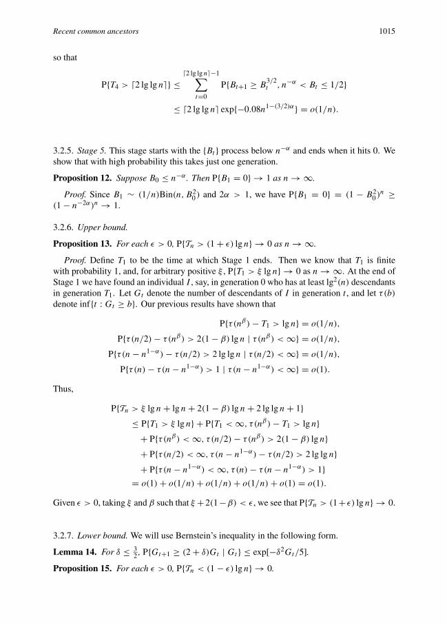
3.2.5. Stage 5. This stage starts with the {Bt } process below n−α and ends when it hits 0. Weshow that with high probability this takes just one generation.

Proposition 12. Suppose B0 ≤ n−α . Then P{B1 = 0} → 1 as n→ ∞.

Proof. Since B1 ∼ (1/n)Bin(n, B20 ) and 2α > 1, we have P{B1 = 0} = (1 − B2

0 )n ≥

(1 − n−2α)n → 1.

3.2.6. Upper bound.

Proposition 13. For each ε > 0, P{Tn > (1 + ε) lg n} → 0 as n→ ∞.

Proof. Define T1 to be the time at which Stage 1 ends. Then we know that T1 is finitewith probability 1, and, for arbitrary positive ξ , P{T1 > ξ lg n} → 0 as n → ∞. At the end ofStage 1 we have found an individual I , say, in generation 0 who has at least lg2(n) descendantsin generation T1. Let Gt denote the number of descendants of I in generation t , and let τ(b)denote inf{t : Gt ≥ b}. Our previous results have shown that

P{τ(nβ)− T1 > lg n} = o(1/n),P{τ(n/2)− τ(nβ) > 2(1 − β) lg n | τ(nβ) <∞} = o(1/n),

P{τ(n− n1−α)− τ(n/2) > 2 lg lg n | τ(n/2) <∞} = o(1/n),P{τ(n)− τ(n− n1−α) > 1 | τ(n− n1−α) <∞} = o(1).

Thus,

P{Tn > ξ lg n+ lg n+ 2(1 − β) lg n+ 2 lg lg n+ 1}≤ P{T1 > ξ lg n} + P{T1 <∞, τ (nβ)− T1 > lg n}

+ P{τ(nβ) <∞, τ (n/2)− τ(nβ) > 2(1 − β) lg n}+ P{τ(n/2) <∞, τ (n− n1−α)− τ(n/2) > 2 lg lg n}+ P{τ(n− n1−α) <∞, τ (n)− τ(n− n1−α) > 1}

= o(1)+ o(1/n)+ o(1/n)+ o(1/n)+ o(1) = o(1).Given ε > 0, taking ξ and β such that ξ +2(1−β) < ε, we see that P{Tn > (1+ ε) lg n} → 0.

3.2.7. Lower bound. We will use Bernstein’s inequality in the following form.

Lemma 14. For δ ≤ 32 , P{Gt+1 ≥ (2 + δ)Gt | Gt } ≤ exp[−δ2Gt/5].

Proposition 15. For each ε > 0, P{Tn < (1 − ε) lg n} → 0.

1016 J. T. CHANG

Proof. Fix ε ∈ (0, 1). Proceeding forward in time from generation 0, we want to show thatthe probability that none of the individuals in generation 0 becomes a CA beforegeneration �(1 − ε) lg n� tends to 1 as n → ∞. Define G0 = 1 and (Gt+1 | Gt, . . . ,G0) ∼Bin(n, 2Gt/n − (Gt/n)2). Here we think of Gt as the number of descendants of individualI0,1 in generation t . Fix r ∈ (0, ε) so that 2(1−r)/(1−ε) ∈ (2, 3.5). Let {Gt } evolve like {Gt }except that it is truncated (or ‘reflected’) below at the value �nr�. That is,

(Gt+1 | Gt , . . . , G0) ∼ max

Bin

n, 2Gt

n−

(Gt

n

)2 , �nr�

.

Defining τGn = inf{t : Gt = n} and τ Gn = inf{t : Gt = n}, obviously P{τGn ≥ u} ≥ P{τ Gn ≥ u}for all u. Since G0 = �nr�, if τ Gn ≤ �(1 − ε) lg n�, then we must have Gt+1 ≥ Gt2(1−r)/(1−ε)for some t < �(1 − ε) lg n�. Defining δ = 2(1−r)/(1−ε) − 2 ∈ (0, 3

2 ), by Lemma 14 theprobability of this is at most

�(1 − ε) lg n� exp(−δ2�nr�/5),which is o(1/n) as n → ∞. Thus, we have shown that the probability that individual I0,1 hasbecome a CA by generation �(1 − ε) lg n� is o(1/n). So the event that at least one of the nindividuals in generation 0 becomes a CA by generation �(1 − ε) lg n� is a union of n suchevents of probability o(1/n), and hence has probability that tends to 0 as n→ ∞.

3.3. Proof of Theorem 2

Idea. The idea of the proof is as follows. Define tn = �(ζ−ε) lg n� and un = �(ζ+ε) lg n�. Foreach i = 1, . . . , n, the process {Git : t = 0, 1, . . . } follows the descendants of individual I0,i .We are waiting until all n of the processes {G1

t }, . . . , {Gnt } have reached either 0 or n (somewill reach 0 and some will reach n). The key ingredient of the argument is this assertion:with high probability, there are many i’s such that Gitn ∈ [1, lg2(n)] and there is no i such thatGiun ∈ [1, lg2(n)]. This follows from Lemma 3 together with an analysis of the Galton–Watsonprocess with offspring distribution Poisson(2). For an upper bound, consider the situation attime un. Some of the processes have become extinct and reached 0, and we are just waitingfor the other, non-extinct processes to reach 0 or n. The key assertion says that with highprobability, all of the non-extinct processes have reached values above lg2(n). This level ishigh enough so that with high probability these processes will all increase predictably andreach n within (1 + ε) lg n additional generations; this was shown in the proof of Theorem 1.So with high probability, Un ≤ un + (1 + ε) lg n. For a lower bound, the key assertion statesthat with high probability many of the n processes are in the interval [1, lg2(n)] at time tn. It isvery unlikely that all of these will go extinct. Furthermore, since these processes are startingfrom at most lg2(n) at time tn, with high probability it will take more than (1−ε) lg n additionalgenerations for any of them to reach n. So Un > tn + (1 − ε) lg n with high probability.

3.3.1. A branching process result.

Lemma 16. Let {Yt } be a Galton–Watson process whose offspring distribution is Poisson withmean 2, starting at Y0 = 1. Define γ as in Theorem 2, and let b1, b2, . . . be positive integerssatisfying lg(bt ) = o(t) as t → ∞. Then

limt→∞

1

tlg P{1 ≤ Yt ≤ bt } = lg(γ ) ≈ −1.29911.

Recent common ancestors 1017

Proof. We use a number of results from chapter 1 of Athreya and Ney (1972). First, theMonotone Ratio Lemma says that for each k there is a λk <∞ such that

P{Yt = k}P{Yt = 1} ↑ λk as t → ∞.

Also,

4(s) :=∞∑k=1

λksk <∞ for all s ∈ (0, 1).

Finally, using the notation and facts collected in Lemma 4, we have

P{Yt = 1} = ψ ′t (0) = ψ ′[ψt−1(0)]ψ ′

t−1(0) = ψ ′[ψt−1(0)] P{Yt−1 = 1},so that

P{Yt = 1}P{Yt−1 = 1} ↑ ψ ′(ρ) = 2ρ = γ.

In particular, (1/t) lg P{Yt = 1} ↑ lg γ .

For s ∈ (0, 1),bt∑k=1

P{Yt = k} ≤ P{Yt = 1}bt∑k=1

λk

≤ P{Yt = 1}s−btbt∑k=1

λksk

≤ P{Yt = 1}s−bt4(s). (8)

If we take s close to 1 (e.g. s = 1 − b−1t , say), then the term s−bt will remain bounded and

present no difficulty. So we would like to know how 4(s) grows as s ↑ 1.Define ϕ to be the inverse function ψ−1, and ϕk to be the k-fold composition ϕ ◦ · · · ◦ ϕ.

By equation (6) on page 12 of Athreya and Ney (1972), for each s ∈ (ρ, 1),4(ϕ(s)) = γ−1[4(s)−4(e−2)] ≤ γ−14(s).

Therefore, since ρ < 12 < ϕ(

12 ) < ϕ2(

12 ) < · · · < 1,

4(ϕk(12 )) ≤ γ−k4( 12 ).

However, since ψ ′(1) = 2, we may choose a number 7 so that

ϕk(12 ) ≥ 1 − (1.9)−k7

and, therefore,4(1 − (1.9)−k7) ≤ γ−k4( 12 )

hold for all sufficiently large k. From this, it follows that

4(1 − y) ≤ 4( 12 )(y/7)(lgγ )/(lg 1.9) ≤ y2 lgγ

holds for all sufficiently small positive y.

1018 J. T. CHANG

Now substituting s = 1 − b−1t in (8), there is a finite constant C such that

bt∑k=1

P{Yt = k} ≤ Cγ t4(1 − b−1t ) ≤ Cγ tb2 lg(1/γ )

t .

Thus, as long as bt grows subgeometrically, that is, lg(bt ) = o(t), we have

limt→∞1

tlg P{1 ≤ Yt ≤ bt } ≤ lg(γ ).

Combining this with the fact that limt→∞(1/t) lg P{Yt = 1} = lg(γ ) completes the proof.

3.3.2. Upper bound.

Lemma 17. Let I0,i denote individual i in generation 0. DefineGit to be the number of descen-dants of I0,i in generation t; in particular, Gi0 = 1 for all i = 1, . . . , n. Also define

τ i0,b = inf{t : Git = 0 or Git ≥ b},and let

An =n⋃i=1

{τ i0,lg2 n

> (ζ + ε) lg n}. (9)

Then P(An)→ 0 as n→ ∞.

Proof. Define τY0b = inf{t : Yt = 0 or Yt ≥ b}. Since {τY0b > t} ⊆ {1 ≤ Yt < b}, Lemma 16and (3) give

lim1

tlg P{τ i0b > t} ≤ lg(γ ) if lg(b) = o(t) and tb2 = o(n). (10)

Letting ε > 0 and applying (10) to t = (ζ + ε)(lg n) and b = lg2(n) gives

lg P{τ i0,lg2(n)

> (ζ + ε)(lg n)} ≤ (lg(γ )+ δ)(ζ + ε)(lg n)

for all δ and all sufficiently large n. Taking δ sufficiently small, from the definition of ζ we seethat

P{τ i0,lg2(n)

> (ζ + ε)(lg n)} = o(1/n) as n→ ∞,so that P(An) = o(1).

We have shown that, with high probability, all individuals in generation 0 have either nodescendants or more than lg2(n) descendants in generation �(ζ + ε) lg n� for ε > 0. Next wewill show that for any given ε > 0, with high probability, each individual having more thanlg2(n) descendants in generation �(ζ + ε) lg n� becomes a CA within (1 + ε) lg n additionalgenerations. Most of the work required to prove this has already been done in the proof ofTheorem 1; the extra ingredient is the following lemma, which takes a closer look at ‘Stage 5’.We retain the definition Bt = 1 − (Gt/n) from above.

Lemma 18. Let α ∈ ( 12 , 23 ) and take k(α) > 1/(2α − 1). Suppose that B0 ≤ n−α and define

T5 = inf{t : Bt = 0}. Then P{T5 > k(α)} = o(1/n) as n→ ∞.

Recent common ancestors 1019

Proof. Since (Bt+1 | Bt) ∼ (1/n)Bin(n, B2t ), on the event {Bt ≤ n−α} we have

P{Bt+1 > 0 | Bt } = 1 − (1 − B2t )n

≤ 1 − (1 − 2nB2t ) = 2nB2

t ≤ 2n1−2α,

where the first inequality holds for sufficiently large n (since α > 12 implies that nB2

t isarbitrarily small for sufficiently large n). In particular,

P{0 < Bt+1 ≤ n−α | 0 < Bt ≤ n−α} ≤ 2n1−2α for sufficiently large n. (11)

Next, by Bernstein’s inequality, on the event {Bt ≤ n−α},

P{Bt+1 > n−α | Bt } = P

{1

nBin(n, B2

t ) > B2t + (n−α − B2

t ) | Bt}

≤ exp

[ −n2(n−α − B2t )

2

2nB2t (1 − B2

t )+ (2/3)n(n−α − B2t )

]

≤ exp

[ −n2−2α

2n1−2α + (2/3)n1−α

].

Since the exponent is asymptotic to −( 32 )n1−α , clearly

P{Bt+1 > n−α | Bt } ≤ exp[−n1−α] on {Bt ≤ n−α}

for sufficiently large n. Assuming that B0 ≤ n−α ,

k⋃t=0

{Bt > n−α} ⊆k−1⋃t=0

{Bt ≤ n−α, Bt+1 > n−α}.

Therefore, since

P{Bt ≤ n−α, Bt+1 > n−α} = E[{Bt ≤ n−α}P{Bt+1 > n

−α | Bt }] ≤ exp[−n1−α],

we obtain

P

[k⋃t=0

{Bt > n−α}]

≤ k exp[−n1−α]. (12)

Thus, using (11) and (12),

P{T5 > k} ≤ P

(k⋃t=0

{Bt > n−α})

+ P

(k⋂t=0

{0 < Bt ≤ n−α})

≤ k exp[−n1−α] + (2n1−2α)k.

Applying this to k = k(α) > 1/(2α − 1) gives the desired result.

1020 J. T. CHANG

Proof of the upper bound in Theorem 2. Let Un denote the time at which everyone fromgeneration 0 has become a CA or extinct. Recall the definition of An from (9), and let τ i(b) =inf{t : Git ≥ b}. Since

{Un > (1 + ζ + 2ε) lg n} ⊆ An ∪ [Acn ∩ {Un > (1 + ζ + 2ε) lg n}]

⊆ An ∪n⋃i=1

{τ i(lg2 n) ≤ (ζ + ε) lg n, τ i(n) > (1 + ζ + 2ε) lg n},

to show that P{Un > (1 + ζ + 2ε) lg n} = o(1), by Lemma 17 it suffices to show that

P{τ 1(lg2 n) ≤ (ζ + ε) lg n, τ 1(n) > (1 + ζ + 2ε) lg n} = o(1/n).To see this, observe that the results of Stages 2 through 4 from the proof of Theorem 1 showthat

P{τ 1(nβ)− τ 1(lg2 n) > lg n | τ 1(lg2 n) <∞} = o(1/n),P{τ 1(n/2)− τ 1(nβ) > 2(1 − β) lg n | τ 1(nβ) <∞} = o(1/n),

P{τ 1(n− n1−α)− τ 1(n/2) > 2 lg lg n | τ 1(n/2) <∞} = o(1/n),and Lemma 18 gives

P{τ 1(n)− τ 1(n− n1−α) > k(α) | τ 1(n− n1−α) <∞} = o(1/n).Consequently,

P{τ 1(n)− τ 1(lg2 n) > lg n+ 2(1 − β) lg n+ 2 lg lg n+ k(α) | τ 1(lg2 n) <∞} = o(1/n).Choosing β sufficiently close to 1, we see that for any given ε > 0,

P{τ 1(n)− τ 1(lg2 n) > (1 + ε) lg n | τ 1(lg2 n) <∞} = o(1/n).Thus,

P{τ 1(lg2 n) ≤ (ζ + ε) lg n, τ 1(n) > (1 + ζ + 2ε) lg n}≤ P{τ 1(lg2 n) <∞, τ 1(n)− τ 1(lg2 n) > (1 + ε) lg n} = o(1/n),

as desired.

3.3.3. Lower bound. The proof goes as follows. First we show that at time tn = �(ζ − ε) lg n�,there are many individuals i who have Gitn ∈ [1, lg2 n]. The probability that all of theseindividuals eventually become extinct is negligibly small. In the probable event that not all ofthese individuals become extinct, the time Un must wait for at least one of them to become aCA. From the previous results we know that this will take an additional (1−ε) lg n generations.

Here is some notation that will be used throughout the proof. Let tn denote �(ζ − ε) lg n�.For 1 ≤ i ≤ n, define Ji to be the event {Git ∈ [1, lg2 n] for all t ≤ tn}; we will alsodenote by Ji the indicator random variable corresponding to this event. Thus, Ji = 1 meansthat individual i in generation 0 does not become extinct by time tn and that the number ofdescendants of this individual also remains relatively small (no more than lg2(n)) up to time tn.

Recent common ancestors 1021

At time tn these individuals still have a chance to become CAs, but they have not yet mademuch progress toward doing so. The number of such individuals is Nn = ∑n

i=1 Ji .The next lemma shows that there is little dependence between the numbers of descendants

of different individuals in the early stages of the process. The lemma gives an upper bound ona probability; a similar lower bound may be obtained, but it is not needed in the remainder ofthe proof.

Lemma 19. P(J1J2) ≤ [P(J1)]2(1 + o(1)) as n→ ∞.

Proof. Consider individuals I0,1 and I0,2, that is, individuals 1 and 2 in generation 0. LetAt denote the number of individuals in generation t who are descendants of I0,1 but not ofI0,2. Let Ct denote the number of individuals in generation t who are descendants of I0,2but not of I0,1. Let Bt denote the number of individuals in generation t who are descendantsof both I0,1 and I0,2. This notation is local to this proof; in particular, Bt has a differentmeaning here than it did in the proof of Theorem 1. So G1

t = At + Bt and G2t = Ct + Bt .

Letting Ht = (At , Bt , Ct ), the process {Ht } is a Markov chain. For convenience we use thenotation PH (at , bt , ct ) for P{At = at , Bt = bt , Ct = ct }, PH (at+1, bt+1, ct+1 | at , bt , ct ) forP{At+1 = at+1, Bt+1 = bt+1, Ct+1 = ct+1 | At = at , Bt = bt , Ct = ct }, and so on.

We begin by observing that

P(J1J2) ∼ P(J1J2{Bt = 0 for all t ≤ tn}). (13)

This is easy to see intuitively: If At and Ct are both bounded by lg2(n) and Bt = 0, then theconditional probability that Bt+1 > 0 is at most 2AtCt/n = O(lg4(n)/n). This suggests thatfor each s ≤ tn, given the event J1J2, the conditional probability that Bt is positive for the firsttime at t = s isO(lg4(n)/n). Adding these probabilities over all s ≤ tn = O(lg n) would thengive

P(Bt > 0 for some t ≤ tn | J1J2) = O(lg5(n)/n).

This is correct, and the relation

P(J1J2) = P(J1J2{Bt = 0 for all t ≤ tn})[1 +O

(lg5(n)

n

)]

follows from a rather tedious calculation whose details we omit. The calculation bounds ratiosof binomial probabilities in similar way to an argument that is given later in this proof.

Letting Ln denote the interval [1, lg2 n], we want an upper bound on the probability

P(J1J2{Bt = 0 for all t ≤ tn})=

∑a1∈Ln

· · ·∑atn∈Ln

∑c1∈Ln

· · ·∑ctn∈Ln

PH (a1, 0, c1, a2, 0, c2, . . . , atn , 0, ctn)

=∑

a1,c1∈Ln

PH (a1, 0, c1)∑

a2,c2∈Ln

PH (a2, 0, c2 | a1, 0, c1) · · ·∑

atn ,ctn∈Ln

PH (atn, 0, ctn | atn−1, 0, ctn−1).

1022 J. T. CHANG

Defining

αs = 2asn

− as(as + 2cs)

n2 ,

βs = 2ascsn2 ,

and

γs = 2csn

− cs(cs + 2as)

n2 ,

we may write

PH (at , 0, ct | at−1, 0, ct−1) = P{Bin(n, αt−1) = at }P{Bin

(n− at , γt−1

1 − αt−1

)= ct

}

× P

{Bin

(n− at − ct , βt−1

1 − αt−1 − γt−1

)= 0

}.

We want to compare this to the analogous probability for two independent {Gt } processes, thatis, to

PG(at | at−1)PG(ct | ct−1) = P{Bin(n, αt−1 + βt−1) = at } P{Bin(n, γt−1 + βt−1) = ct }.The ratio

PH (at , 0, ct | at−1, 0, ct−1)

PG(at | at−1)PG(ct | ct−1)(14)

is the product of three terms:

P{Bin(n, αt−1) = at }P{Bin(n, αt−1 + βt−1) = at } , (15)

P{Bin(n− at , γt−1/(1 − αt−1)) = ct }P{Bin(n, γt−1 + βt−1) = ct } , (16)

and

P{Bin

(n− at − ct , βt−1

1 − αt−1 − γt−1

)= 0}. (17)

We bound the third term (17) simply by 1; in fact it is close to 1. The term (15) is

αatt−1(1 − αt−1)

n−at(αt−1 + βt−1)at (1 − αt−1 − βt−1)n−at

≤(

1 + βt−1

1 − αt−1 − βt−1

)n

= 1 +O(

lg4(n)

n

),

sinceβt−1

1 − αt−1 − βt−1∼ βt−1 ≤ 2 lg4(n)

n2

Recent common ancestors 1023

for at−1, ct−1 ≤ lg2(n). By a similar calculation, (16) is also 1+O (n−1 lg4(n)

). Multiplying,

we obtainPH (at , 0, ct | at−1, 0, ct−1)

PG(at | at−1)PG(ct | ct−1)= 1 +O

(lg4(n)

n

).

Thus,

P(J1J2{Bt = 0 for all t ≤ tn})=

∑a1,c1∈Ln

PH (a1, 0, c1)∑

a2,c2∈Ln

PH (a2, 0, c2 | a1, 0, c1) · · ·∑

atn ,ctn∈Ln

PH (atn, 0, ctn | atn−1, 0, ctn−1)

≤∑

a1,c1∈Ln

PG(a1 | 1)PG(c1 | 1)∑

a2,c2∈Ln

PG(a2 | a1)PG(c2 | c1) · · ·

∑atn ,ctn∈Ln

PG(atn | atn−1)PG(ctn | ctn−1)

[1 +O

(lg4(n)

n

)]tn

=∑

at ,...,atn∈Ln

PG(a1 | 1)PG(a2 | a1) · · · PG(atn | atn−1)

∑ct ,...,ctn∈Ln

PG(c1 | 1)PG(c2 | c1) · · · PG(ctn | ctn−1)

[1 +O

(lg4(n)

n

)]tn

=[P{G1

t ∈ Ln for all t ≤ tn}]2

[1 +O

(lg5(n)

n

)]

= [P(J1)]2[1 +O

(lg5(n)

n

)].

This completes the proof.

Lemma 20. Nn → ∞ in probability as n→ ∞.

Proof. We will show that the mean and standard deviation of Nn satisfy ENn → ∞ andSD(Nn) = o(E(Nn)). To see that ENn = nPJ1 → ∞, begin with (3), which gives

P(J1) ∼ P{Yt ∈ [1, lg2(n)] for all t ≤ tn}.This last probability is very close to P{Ytn ∈ [1, lg2(n)]}. Indeed, the difference

P{Ytn ∈ [1, lg2(n)]} − P{Yt ∈ [1, lg2(n)] for all t ≤ tn}= P{Ytn ∈ [1, lg2(n)], Yt > lg2(n) for some t < tn}, (18)

is the probability that the Y process exceeds lg2(n) some time before tn but then decreases tobe below lg2(n) at time tn. Since the Bernstein inequality applied to the Poisson distributiongives

P{Yt+1 ≤ Yt | Yt } ≤ exp[−( 314 )Yt ] ≤ exp[−( 3

14 ) lg2(n)] on {Yt > lg2(n)},

1024 J. T. CHANG

the difference (18) is bounded by tn exp[−(3/14) lg2(n)] = o(1/n). By Lemma 16,

lg P{Ytn ∈ [1, lg2(n)]}(ζ − ε) lg n ∼ 1

tnlg P{Ytn ∈ [1, lg2(n)]} → lg γ = −1

ζ,

which implies that nP{Ytn ∈ [1, lg2(n)]} → ∞. Thus,

nP(J1) ∼ nP{Yt ∈ [1, lg2(n)] for all t ≤ tn} = n[P{Ytn ∈ [1, lg2(n)]} + o(1/n)] → ∞.Finally, to see that SD(Nn) = o(E(Nn)), we apply Lemma 19 to obtain

Var(Nn) = E(N2n )− (ENn)2 = nPJ1 + n(n− 1)P(J1J2)− (nPJ1)

2

≤ nPJ1 + n(n− 1)[P(J1)]2(1 + o(1))− (nPJ1)2

= o(n2(PJ1)2) = o((ENn)2).

Proof of the lower bound in Theorem 2. DefiningWn = {i : Gitn ∈ [1, lg2(n)]}, we have

P{Un ≤ tn + (1 − ε) lg(n)}≤ P{Wn = ∅} + P{eventual extinction for all i ∈ Wn}

+ P{Gi�tn+(1−ε) lg(n)� = n for some i ∈ Wn}. (19)

The cardinality of the setWn isNn. SinceNnP→ ∞, clearly the probability that all individuals

{I0,i : i ∈ Wn} eventually become extinct converges to 0; this is an easy consequence of resultsabout extinction probabilities of Kammerle (1991) or Mohle (1994). So it remains to show thatthe last probability in (19) tends to 0. To see this, taking i ∈ Wn, observe that for the event{Gi�tn+(1−ε) lg(n)� = n} to occur the {Git } process must go from below lg2(n) at time tn to n at

time �tn + (1 − ε) lg(n)�. That is, the process must go from below lg2(n) to n within a timespan of at most (1 − ε) lg(n) generations. However, by the proof of Proposition 15, we knowthat this has probability o(1/n), so that, taking the union over i ∈ Wn gives a total probabilityof o(1).

4. Discussion

A motivation behind this study was the interest surrounding the idea of all of mankindhaving a recent common ancestor. In thinking about a mathematical treatment of that idea, itseemed natural to remove the restriction to the maternal line and consider a two-parent model.

We have seen that CAs occur very recently in the two-parent model studied here. Themost recent CA occurs, with high probability, about lg n generations ago. Within 1.77 lg ngenerations, with high probability, all individuals who are not extinct are CAs. These resultsdescribe the behavior of populations satisfying certain assumptions of random mating and soon. If our world really satisfied such assumptions, the anthropological excitement about therecentness of mitochondrial Eve would be misplaced: in only a tiny fraction of the time backto mitochondrial Eve, common ancestors of mankind would abound, and in fact a randomlychosen individual would be a CA with probability about 0.8.

If we wish to understand analogous questions in more complicated models that could betteraddress phenomena such as the evolution of mankind, further study is required. For example,

Recent common ancestors 1025

the absence of geographic structure is a key feature limiting the applicability of the modelstudied here to such situations.

Conclusions based on analyses of simple models that ignore geographic considerationsare commonly seen in the scientific discourse about the evolution of mankind. As a typicalexample, the abstract of Ayala’s (1995) paper states

The theory of gene coalescence suggests that, throughout the last 60 million years,human ancestral populations have had an effective size of 100 000 individuals orgreater.

The investigation of ‘Y -chromosome Adam’ by Dorit et al. (1995) is another interestingexample. Such analyses rely strongly on the basic predictions of standard coalescent theory:n generations for the expected coalescence time of a pair of genes among a population of ngenes, and 2n generations for the expected coalescence of the whole population.

On the other hand, it is doubtful that anyone would seriously entertain the two-parentanswer of lg n for a CA in the context of the evolution of mankind. This raises conceptualquestions. On what basis do we draw insight from the analysis of a one-parent model, whenanalysis of an analogous two-parent model leads to results we find implausible? Whereas theanswer 2n given by a haploid model for the ‘Eve’ coalescence time may not be so obviouslyinapplicable in a given situation, the two-parent model’s CA time of lg n may well be.

A possible source of comfort when confronting doubts about the realism of the assumptionsunderlying the standard coalescent model is the body of results about ‘robustness’ of thecoalescent. Kingman (1982b) showed that the coalescent arises as a limiting genealogy ina whole class of models that includes Wright–Fisher and other classical models. However, thisclass of models assumes symmetries (related to exchangeability) that are typically violated inmodels incorporating population subdivision or geographic structure.

The two-parent results highlight the strong consequences that can follow from assumingmodels of the Wright–Fisher type, and in particular from assumptions of random mating.The mathematical conclusions of these models may not be as robust as one might hope, andmodels that ignore violations of assumptions such as random mating can easily lead to absurdestimates. Such unrealistically simple assumptions form a natural starting point for this firstinvestigation of MRCAs in two-parent models, as it seems appropriate to begin with a directanalog of a classical model that lies at the foundation of the one-parent theory. But there ismuch that could be done to generalize this work.

In the context of one-parent models, a substantial literature investigates departures fromthe simplest assumptions of the classical models. In particular, models allowing populationsize to vary over time and models incorporating various forms of population subdivision andgeographic structure are all under continuing investigation. See, for example, the recentcollection of papers edited by Donnelly and Tavare (1997), which gives a fine overview ofrecent work.

Mohle (1997) has considered the effect of varying population size in some genetic modelsdistinguishing males and females. Mohle’s focus is on the genetic question of ultimate fixationof an allele, so that the two-sex, diploid aspect of the models does not fundamentally affectthe nature of the results, although it complicates the proofs; the results match earlier resultsof Donnelly (1986) about variable population size versions of the standard one-parent models.Aside from this work, generalizations of the standard assumptions remain to be investigated intwo-parent models.

1026 J. T. CHANG

Acknowledgements

I am grateful to Russell Lyons, Robin Pemantle, Yuval Peres, and Peter Winkler for helpfuldiscussions about this work. Some of these discussions took place at the first summer work-shop of the Institute for Elementary Studies in Pinecrest, California; I would like to thankRobin Pemantle for inviting me and for hosting a wonderful meeting.

References

Athreya, K. B. and Ney, P. (1972). Branching Processes. Springer, NewYork.Ayala, F. J. (1995). The myth of Eve: molecular biology and human origins. Science 270, 1930–1936.Bernstein, S. (1946). The Theory of Probabilities. Gastehizdat, Moscow.Cann, R. L., Stoneking, M. and Wilson, A. C. (1987). Mitochondrial DNA and human evolution. Nature 325,

31–36.Donnelly, P. (1986). Genealogical approach to variable-population-size models in population genetics. J. Appl.

Prob. 23, 283–296.Donnelly, P. and Tavare, S. (eds.) (1997). Progress in Population Genetics and Human Evolution. Springer,

NewYork.Dorit, R. L., Akashi, H. and Gilbert, W. (1995). Absence of polymorphism at the ZFY locus on the human Y

chromosome. Science 268, 1183–1185.Griffiths, R. and Marjoram, P. (1997). An ancestral recombination graph. In Progress in Population Genetics

and Human Evolution, eds. S. Tavare and P. Donnelly, Springer, NewYork, pp. 257–270.Hudson, R. R. (1983). Properties of a neutral allele model with intragenic recombination. Theoret. Popn. Biol. 23,

183–201.Hudson, R. R. (1990). Gene genealogies and the coalescent process. Oxford Surveys in Evolutionary Biology 7,

1–44.Kammerle, K. (1989). Looking forwards and backwards in a bisexual model. J. Appl. Prob. 27, 880–885.Kammerle, K. (1991). The extinction probability of descendants in bisexual models of fixed population size.

J. Appl. Prob. 28, 489–502.Kingman, J. F. C. (1982a). Exchangeability and the evolution of large populations. In Exchangeability in Probability

and Statistics, eds. G. Koch and F. Spizzichino, North-Holland, NewYork, pp. 97–112.Kingman, J. F. C. (1982b). On the genealogy of large populations. In Essays in Statistical Science, eds. J. Gani and

E. J. Hannan (J. Appl. Prob. 19A,). Applied Probability Trust, Sheffield, UK, pp. 27–43.Mohle, M. (1994). Forward and backward processes in bisexual models with fixed population sizes. J. Appl. Prob.

31, 309–332.Mohle, M. (1997). Fixation in bisexual models with variable population sizes. J. Appl. Prob. 34, 436–448.Paabo, S. (1995). TheY chromosome and the origin of all of us (men). Science 268, 1141–1142.Vigilant, L., Stoneking, M., Harpending, H., Hawkes, K. and Wilson, A. C. (1991). African populations

and the evolution of human mitochondrial DNA. Science 253, 1503–1507.