Recent Results on the Regularization of Fourier Polynomials

D. de Falco, M. Frontini, and L. Gotusso

Mathematics Department Polytechnic of Milan Piazza L. da Vinci 32, 20133 Milano, Italy

ABSTRACT

In a recent paper we presented for two particular cases a unifying approach to the regularization of Fourier polynomials. More precisely, we proved that the regularized polynomials obtained by using the convolution of the given function f(x) with the uniform probability density or with the Gaussian probability den- sity are the same as the ones obtained by minimizing the functional:

where (1 . (1 is the L2 norm, Fc) . IS the rth derivative of the Fourier polynomial F,(X), f(x) is a given function with Fourier coefficients ck, and or are suitable weights. In both cases we have given explicit expressions of the weights err in their dependence on a scalar parameter 7.

In this paper we prove that this unifying approach may be extended to a wide class of convolution kernel. A characterization of this class is also given.

1. INTRODUCTION

It is well known [l, 2] that Gibbs’ phenomenon arises when we ap- proximate in the interval [-n, n) a discontinuous periodic function f(z) of period 27r by Fourier polynomials.

Many techniques have been proposed in the past in order to avoid Gibbs’ phenomenon, Fejer’s sums, the sigma-factor method, or the convolution of f(z) with a suitable function g(z).

More recently, in [3], a new approach for the regularization of Fourier

APPLIED MATHEMATICS AND COMPUTATION 66:1-8 (1994) 1

@ Elsevier Science Inc., 1994 655 Avenue of the Americas, New York, NY 10010 0096-3003/94/$7.00

2 D. DE FALCO, M. FRONTINI, AND L. GOTUSSO

polynomials was proposed based on the minimization of the following func- tional

In [3] it was proven that when

the Fourier coefficients of the regularized polynomial are given by

c;=cke , -(TIC)‘. k = 0,+1,*2,. . ) fn. (2) In [4] we proved that the regularized Fourier polynomials obtained by

minimizing (1) with the weights (la) are the same as those obtained by con- sidering the convolution of the function f(x) with the Gaussian probability density.

Furthermore in [l] it was proven that if the weights or in (1) are defined

or = (-qT-l (Z2, - w32rT2r

(2T)! ’ r = 1,2,..., (3)

where B, axe the Bernoulli numbers, then the coefficients of the polynomial which minimizes (1) are given by

k = 0, +1, f2,. . ) fn.

The coefficients defined in (4) are the same as those obtained by convo- lution of f(x) with the uniform probability density, namely by the a-factor method.

Relations (2) and (4) are of the form

C; = Ck$(Tk); k = 0, *l, +2,, . , fn, (5)

where q5(Tk) is an even smooth function of k depending on the parameter r. The preceding results suggested the equivalence of the following three

different approaches to the regularization of Fourier polynomials:

(1)

(2)

(3)

smoothing the Fourier coefficients of F,(z) by attenuation factors of the form (5); convolution of f(x) with a probability density pLT(x) and computation of the first n Fourier coefficients of the regularized function; and minimization of the functional (1) with preassigned weights (T,.

Regularization of Fourier Polynomials

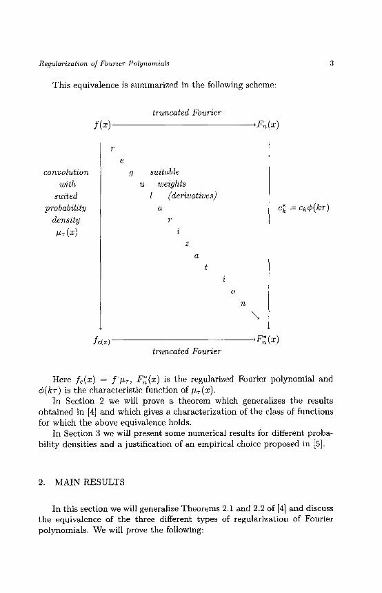
This equivalence is summarized in the following scheme:

f(x)

truncated Fourier

t%(x)

convolution

with

suited

probability

density

k(X)

r

e

9 suitable

21 weights

1 (derivatives)

a

r

i

z

a

c; = c,&(h)

t

i

0

n

\

f c(r) truncated Fourier

+F,‘(x)

Here fC(x) = f’~~, F,*(s) is th e regularized Fourier polynomial and @(/CT) is the characteristic function of ad.

In Section 2 we will prove a theorem which generalizes the results obtained in [4] and which gives a characterization of the class of functions for which the above equivalence holds.

In Section 3 we will present some numerical results for different proba- bility densities and a justification of an empirical choice proposed in [5].

2. MAIN RESULTS

In this section we will generalize Theorems 2.1 and 2.2 of [4] and discuss the equivalence of the three different types of regularization of Fourier polynomials. We will prove the following:

4 D. DE FALCO, M. FRONTINI, AND L. GOTUSSO

THEOREM 2.1. Given f(x), let p7(x) be a family of probability densi- ties depending on the scale parameter T > 0 and let gr(x) be the convolution

gT(X)=f’Pr= j-+m f(t)pT(x - t)dt. --03

Let &(w) be the characteristic function of ~~(5)

&(w)= /+” &x)eiwzdx = I, --oo

where 4(w) is the characteristic function of PI(X).

If the following hypotheses hold,

(4 (ii)

(iii)

then,

PI(X) is even, q(w) = 1/4(w) is analytic inside ]w] 5 R,

all the even derivatives #2’)(O) are nonnegative,

for nr 5 R and for 1 k] < n the coeficients c:(r), defined by

c;(r) = c,&(k) = clc$(kr). (6)

are the coeficients of the Fourier polynomial F,* which minimizes the func-

tional.

J*[F,,rl = Ilf - Fn]12 + &orl~F:)1~2; (7)

where or = r2’+(2’)(0)/(2r)! 2 0. (8)

PROOF. Let ok be the kth Fourier coefficient of the Fourier polyno- mial F,(x) in (7). F or fixed T and n, minimizing J*[F,, r]

minimizing the following function of y = (T_~, . . ,~o,. . . , m) amounts to

(9)

By the orthogonality of the functions eikx within essential additive con-

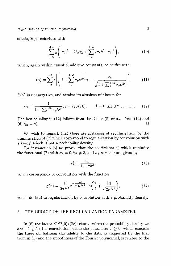
Regularization of Fourier Polynomials

stants, Z(y) coincides with

5

(10)

which, again within essential additive constants, coincides with

3(y) is nonnegative, and attains its absolute minimum for

1

ck = ck@(Tk); Ic = 0, +1,12,. . , fn. (12)

The last equality in (12) follows from the choice (8) or err. From (12) and

(6) ‘)‘k = C;. 0

We wish to remark that there are instances of regularization by the minimization of (7) which correspond to regularization by convolution with a kernel which is not a probability density.

For instance in [6] we proved that the coefficients ci which minimize the functional (7) with ok = O,V’lc # 2, and u2 = c > 0 are given by

ck d= 1+ak4’

which corresponds to convolution with the function

1 g(z) = me-&sin % + m ,

(

I4

1

(13)

(14)

which do lead to regularization by convolution with a probability density.

3. THE CHOICE OF THE REGULARIZATION PARAMETER

In (8) the factor $ czr) (0) / (2r)! characterizes the probability density we are using for the convolution, while the parameter T 1 0, which controls the trade off between the fidelity to the data as requested by the first term in (1) and the smoothness,of the Fourier polynomial, is related to the

6 D. DE FALCO, M. FRONTINI, AND L. GOTUSSO

1 time ud. 2 times u.d.

_)Y[’ J-71 ;I[’ /-’

-4 -2 (:I 2 4 -4 -2 A 2 4

3 times ud

l-

“Il. /‘l

i

-1

-4 -2 A 2 4

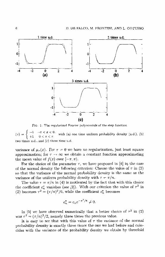
FIG. 1. The regularized Fourier polynomials of the step function

(z)= ,; -7?<z<o.

{ 0<2<7r with (a) one time uniform probability density (u.d.), (b)

two times u.d., and (c) three time u.d.

variance of am. For 7 = 0 we have no regularization, just least square approximation; for r + CXJ we obtain a constant function approximating the mean value of f(z) over (-.ir, r).

For the choice of the parameter r, we have proposed in [4] iq the case of the normal density the following criterion: Choose the value of 7 in (2) so that the variance of the normal probability density is the same as the variance of the uniform probability density with r = n/n.

The value r = n/n in (4) . IS motivated by the fact that with this choice the coefficient ci vanishes (see [2]). With our criterion the value of 72 in

(2) b ecomes 72 = (7r/n)‘/6, while the coefficient cg becomes

12: = c,e --~=I6 # 0,

In 153 we have observed numerically that a better choice of r2 in (2) was r2 = (7r/n)2/2, namely three times the previous value.

It is easy to see that with this value of T the variance of the normal probability density is exactly three times the one we had before and coin- cides with the variance of the probability density we obtain by threefold

Regularization of Fourier Polynomials 7

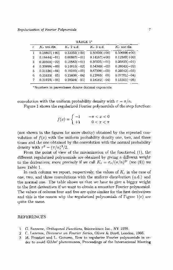
TABLE l*

r K, uni.dis. K, 2 u.d. K, 3 u.d.

1 0.16667(+00) 0,33333(fOO) 0.50000(+00)

2 0.19444( -01) 0.66667(-01) 0.14167(+00)

3 0.20503(-02) 0.10582(-01) 0.30225(-01)

4 0.20999(-03) 0.14815(-02) 0.54349(-02)

5 0.21336(-04) 0.19240(-03) 0.87309(-03)

6 0.21633( -05) 0.23808( -04) 0.12965( -03)

7 0.21923(-06) 0.28504(-05) 0.18182(-04)

K, nor.dis.

0.50000( fO0)

0.12500(+00)

0.20833( -01)

0.26042(-02)

0.26042( -03)

0.21701( -04)

0.15501( -05)

*Numbers in parentheses denote decimal exponents

convolution with the uniform probability density with r = x/n. Figure 1 shows the regularized Fourier polynomials of the step function:

(not shown in the figures for more clarity) obtained by the repeated con-

volution of f(x) with the uniform probability density one, two, and three times and the one obtained by the convolution with the normal probability density with r2 = (7r/n)2/2.

From the point of view of the minimization of the functional (l), the different regularized polynomials are obtained by giving a different weight to the derivatives; more precisely if we call K, = ~~/(n/n)~~ (see (8)) we have Table 1.

In each column we report, respectively, the values of K, in the case of one, two, and three convolutions with the uniform distribution (u.d.) and the normal one. The table shows us that we have to give a bigger weight to the first derivatives if we want to obtain a smoother Fourier polynomial. The values of column four and five are quite similar for the first derivatives and this is the reason why the regularized polynomials of Figure l(c) are quite the same.

REFERENCES

1 G. Sansone, Orthogonal Functions, Interscience Inc., NY 1959. 2 C. Lanczos, Discourse on Fourier Series, Oliver & Boyd, London, 1966. 3 M. Frontini and L. Gotusso, How to regularize Fourier polynomials in or-

der to avoid Gibbs’ phenomenon, Proceedings of the International Meeting

8 D. DE FALCO, M. FRONTINI, AND L. GOTUSSO

Trends in Functional Analysis and Approximation Theory, Atti. Sem. Mat.

Fis. Univ. Modena 39 (1991). 4 D. de Falco, M. Frontini, and L. Gotusso, A unifying approach for

the regularization of Fourier polynomials, Algorithm for Approximation,

Oxford, 1992. 5 M. Frontini and L. Gotusso, A regularization method for discrete Fourier

polynomials, J. Comp. Math. Appl., to appear. 6 M. Frontini and L. Gotusso, Sul lisciaggio di rappresentazioni approssimate

di Fourier, Pubbl. 1st. AppE. Calcolo Ser. III 208 (1981).