Recent Progress in Large Vocabulary Continuous Speech ...cs136a/CS136a_docs/HTK_icassp06_tutorial.pdf · Recent Progress in Large Vocabulary Continuous Speech Recognition: An HTK

Recent Progress in Large Vocabulary ContinuousSpeech Recognition: An HTK Perspective

Mark Gales and Phil Woodland

15 May 2006

Cambridge University Engineering Department

ICASSP 2006 Tutorial

Recent Progress in LVCSR: An HTK Perspective c©Mark Gales & Phil Woodland, 2006

Outline/Introduction• Introduction HTK, BN/CTS tasks, front-ends & normalisation

• Building Blocks Context Dependent HMMs, Language Models and Decoding

• Advanced Techniques

– Discriminative training– Adaptation & adaptive training– Structured covariance models– Lightly supervised training– Confusion networks and system hypothesis combination– System performance examples (BN and CTS)

• Assume some background: basic HMMs (maximum likelihood) & N-gramlanguage models

• HMMs use Gaussian mixture distributions: diagonal covariance matrix

• References are biased towards our own work: not aiming to be complete!

Cambridge UniversityEngineering Department

ICASSP 2006 Tutorial 1


HTK Overview• What is HTK?

– Hidden Markov Model Toolkit– set of tools for training and evaluating HMMs: primarily speech recognition– implementation in ANSI C (Unix & Windows)– includes 300+ page manual [1], tutorial and system build examples– modular structure simplifies extension

• History (1989-)

– Initially developed at Cambridge University (up to V1.5)– ... then Entropic ... (up to V2.2)– Since 2000 back at CU (V3 onwards)– Free to download from web, many 10’s of 1000’s of users– Latest version is V3.4 (an alpha release ...) and V3.3 stable

• Used extensively for reseach (& teaching) at CU

– Built large vocabulary systems for NIST eveluations based on HTK

http://htk.eng.cam.ac.uk/




HTK Features• LPC, MFCC and PLP frontends– cepstral mean/variance normalisation + Vocal Tract length normalisation

• supports discrete and (semi-)continuous HMMs

– diagonal and full covariance models– context dependent cross-word triphones & decision tree state clustering– (embedded) Baum-Welch training

• Viterbi recognition and forced-alignment– support for N-grams and finite state grammars– Includes N-gram generation tools for large datasets– N-best and lattice generation/manipulation

• (C)MLLR speaker/channel adaptation & adaptive training

• From V3.4– Large vocabulary decoder HDecode: separate license– Discriminative training tools, MMI and MPE HMMIRest




BN and CTS Transcription tasks• Conversational Telephone Speech (CTS)

– Conversations on particular topics, normally between strangers– Switchboard corpora, Call Home, Fisher– Casual conversation style– Variable channels (incl. cellular)– Several hundred hours Switchboard1 acoustic training– Two thousand hours of Fisher data (2004 onwards)– Limited matched language model training data– Consists of conversation sides of typically 3 minutes (from 4-wire recordings)

• Broadcast News (BN)– Single audio stream with many talkers, styles, noise conditions, bandwiths– Much of it prepared speech from anchor speakers but some conversational– Need to segment for normalisation/adaptation– For English: 200h of careful transcripts, 1000’s of hours of closed captions– Vocabulary changes with news stories!– Reasonable/large amount of fairly well-matched LM data




Overall Structure of Transcription Systems

P1: Initial Transcription

Adapt

P3x

Lattices

Adapt

P3a

P2: Lattice Generation

Segmentation

Alignment

CNC

1−best

CN

Lattice

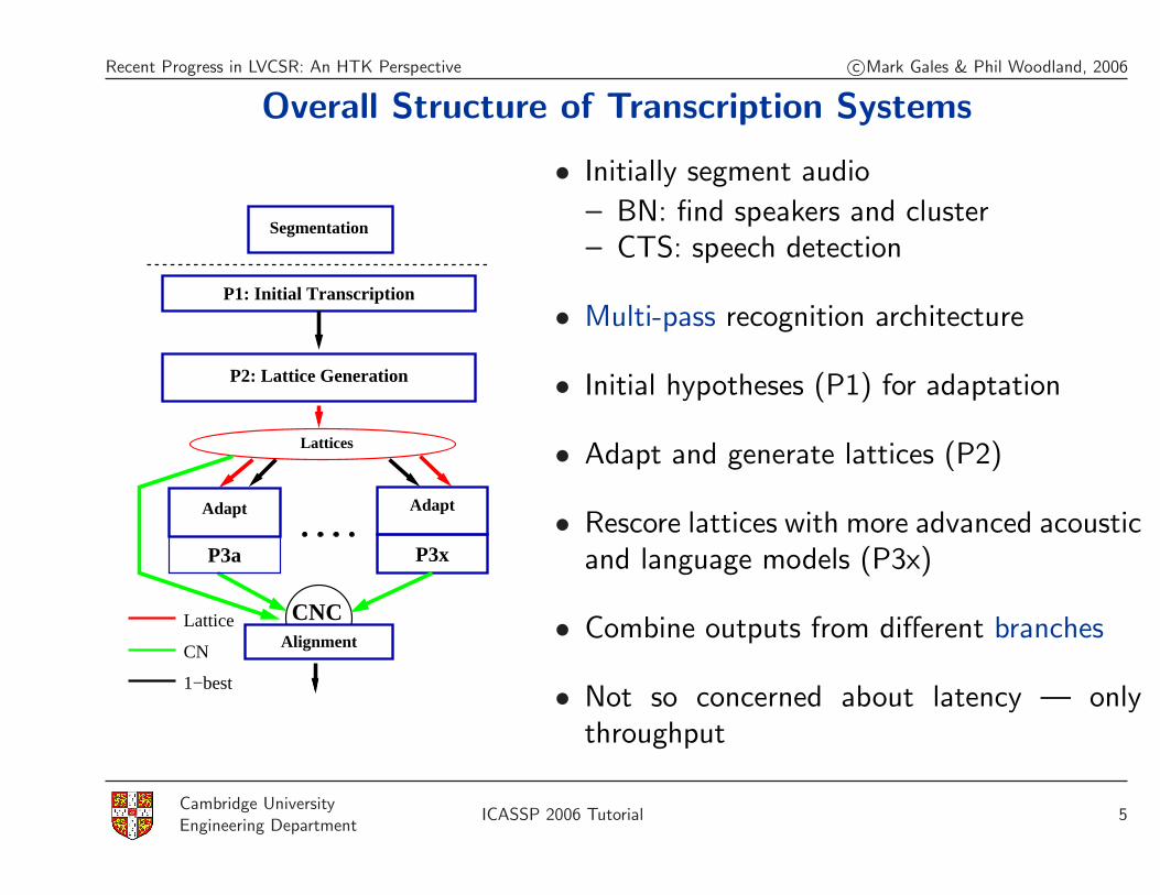
• Initially segment audio

– BN: find speakers and cluster– CTS: speech detection

• Multi-pass recognition architecture

• Initial hypotheses (P1) for adaptation

• Adapt and generate lattices (P2)

• Rescore lattices with more advanced acousticand language models (P3x)

• Combine outputs from different branches

• Not so concerned about latency — onlythroughput




Front-End Parameterisation• Basic front end uses cepstral parameters (typically 12 cepstra + energy/c0)

– Fits with diagonal covariance assumptions

• Add smoothed first/second order derivatives

– Yields 39 dimensional feature vector– Add third-order derivatives if using dimensionality reduction (HLDA)

• HTK supports MFCC cepstra and a form of PLP (perceptual linear prediction)

– PLP implementation uses mel-scale filterbank from standard MFCCs

• Usual to normalise at sentence/segment/side level using CMN/CVN

– Cepstral Mean Normalisation (CMN) removes the average cepstral value:reduces sensitvity to channel

– Cepstral Variance Normalisation (CVN) makes each indiviual coef have fixedvariance: adds some robustness to additive noise




Vocal Tract Length Normalisation

• Aim is to normalise data to account for differences in formant positions due tolength of vocal tract

• Implement via adjusting filter centre frequencies

• Single parameter warp-factor chosen to maximise likelihood

• Procedure

1. Generate word string for e.g. conversation side from P12. Search over warp factors for maximum likelihood warp factor3. Likelihood varies smoothly so can speed up search

• Note that need to account for Jacobian in likelihood comparison

– Use variance normalisation as approximation

• Widely applied for CTS transcription: good gains

– Much harder to get improvements for BN [2]




BN Speaker Segmentation/Clustering

• Divide audio into set of acoustically homogeneous segments– single speaker (or none) & single audio condition

• Initial classification labels data as wide bandwidth (WB) speech, narrow band(NB) speech or pure music/noise using GMMs

• Uses gender-dependent phone recogniser to find short speaker segments

• Uses segment clustering and smoothing rules to generate final segments [3]

• Clustering based on segment Gaussian statistics: bottom-up or top-down [3]– used in acoustic model adaptation

• Alternative procedure (LIMSI) combines segmentation/clustering via GMMs[4]

• Applied after advert removal: looks for repeated audio over several days




Model Structure & Lexicon Design

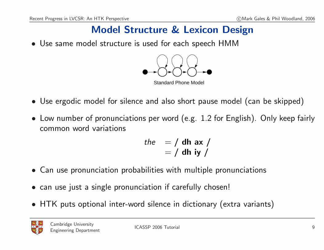
• Use same model structure is used for each speech HMM

Standard Phone Model

• Use ergodic model for silence and also short pause model (can be skipped)

• Low number of pronunciations per word (e.g. 1.2 for English). Only keep fairlycommon word variations

the = / dh ax /= / dh iy /

• Can use pronunciation probabilities with multiple pronunciations

• can use just a single pronunciation if carefully chosen!

• HTK puts optional inter-word silence in dictionary (extra variants)




Context-Dependent Acoustic Models• Phone realisations are too variable to use Context Independent HMMs

• Make many Context Dependent versions of each phone by taking into accountimmediate left and right phonetic context (triphones).

• Can use wider context ±2 yields quinphones/pentaphones

• Contexts can extend across word-boundaries (cross-word triphones)

• Issue: too many parameters / models, and most contexts are very rare

• Parameter-Tying uses the same model / state distribution for different contexts

• Allows the robust estimation of contexts for which there is little data

• Tying at the state-level is more effective than model level

– Top-down decision-tree state tying allows contexts unseen in training to betied.




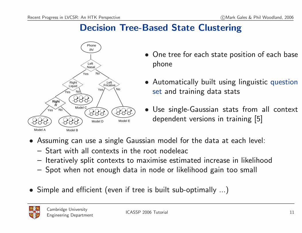
Decision Tree-Based State Clustering

Right/l/

Right/l/

No

Phone/ih/

NasalLeft

RightLiquid

Left Fricative

Model D Model E

Model C

Model BModel A

NoYes

Yes

Yes

Yes NoNo

• One tree for each state position of each basephone

• Automatically built using linguistic questionset and training data stats

• Use single-Gaussian stats from all contextdependent versions in training [5]

• Assuming can use a single Gaussian model for the data at each level:

– Start with all contexts in the root nodeleac– Iteratively split contexts to maximise estimated increase in likelihood– Spot when not enough data in node or likelihood gain too small

• Simple and efficient (even if tree is built sub-optimally ...)




N-Gram Language Modelling

• The Language Model (LM) gives probabilities of sentences

• Use N-gram models so that the probability of a word string w is

P (w) =T∏

k=1

P (wk|wk−1...wk−N+1)

i.e. treat all contexts with the same N − 1 words as equivalent.

• Key issue is data sparsity

– number of trigrams (N = 3 )to cover a 60k word vocabulary is 2.2× 1014!– need to estimate N-grams not seen in training

• For LVCSR use back-off LM to integrate with decoder

– count discounting and back-off e.g. Good-Turing, modified Kneser-Ney

• Use HLM tollkit in HTK or SRILM toolkit to build basic LMs [6]




Vocabulary Coverage

• Need to minimise the number of out-of-vocabulary (OOV) items

– For each OOV word a recogniser typically makes 1.6 word errors [7]

• For English business newspaper text a 5k vocab would typically have a 9%OOV rate; 20k 2% and 65k 0.6%.

• Reduce OOVs if vocabulary tailored for a particular individual or topic

• Vocabulary must be kept “up-to-date” for BN

• For some morphologically productive languages need much larger vocab

– Russian: need 800k vocab for 1% OOV rate– Arabic: need 400k vocab for 1% OOV rate– Alternative is to model sub-word units ...

• For languages such as Chinese word boundaries not given so need to use acharacter to word segmenter




Practical LM build procedure

• Normalisation for each source of LM data (transcripts, web sources etc.)

– remove non-text– sentence segmentation– convert numbers, web addresses etc. to spoken form

• select vocabulary to minimise expected OOV rate

– use most likely words in training– take account of available dictionaries ...

• build LM for each source (selecting N-gram cut-offs)

• merge into a mixture model of N-grams from each source

• mixture weights found by minimising perplexity on dev test data

• prune final model to rely more on back-off structure (entropy pruning) tofurther control size [8]




LM scale factor

• During recognition, combine the LM probability with HMM likelihood

• In theory should just multiply together (or add the logs).

– However HMM likelihood underestimated (independence assumptions)– Need to scale up (raise to a power) the LM probabilties

• Uselog p(O|w) + α log P (w) + β|w|

– α is the language model scale factor– β is the word insertion penalty (|w| means the number of words in w)

• Typically for HTK (natural logs)

– α in range 10 to 16– β in range 0 to −20




Decoding

• Large vocabulary decoders deliver the recognition output

– Find 1-best or N-best / lattice of recognition alternatives– Need to be able to use all acoustic / language models– Ideally want speed ... but flexibility more important in HTK!– HTK V3.4 decoders based on Viterbi-search of static networks

• Small/medium vocabulary HVite

– Encode all problem constraints in the network structure– Linear lexicon– Handle cross-word triphones/bigram LM by full network expansion– Multiple tokens (heads of paths) to represent alternatives in a network state– In LV systems can be used to rescore lattices

• For large vocabulary HDecode need more efficiency

– Use a tree-structured network topology (incl cross-word triphones)




aen

d

ehn

b tih

l

BEN

BIT

BILL

AND

p

AND

pANDBILL

pANDBIT

{ }max

pANDAND

pANDBEN

pANDBIT

pANDBILL

ANDBILLp

ANDBITp

ANDBEN

{ }max

��

��

��

� ��

��

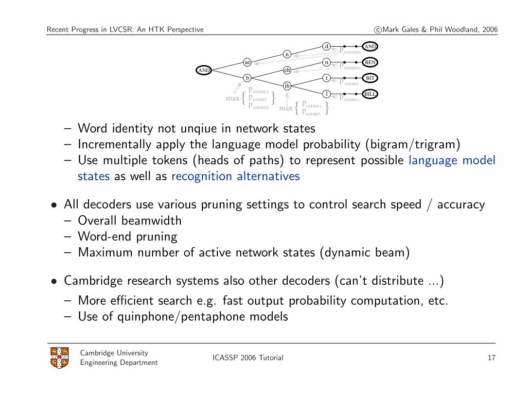
– Word identity not unqiue in network states– Incrementally apply the language model probability (bigram/trigram)– Use multiple tokens (heads of paths) to represent possible language model

states as well as recognition alternatives

• All decoders use various pruning settings to control search speed / accuracy– Overall beamwidth– Word-end pruning– Maximum number of active network states (dynamic beam)

• Cambridge research systems also other decoders (can’t distribute ...)

– More efficient search e.g. fast output probability computation, etc.– Use of quinphone/pentaphone models




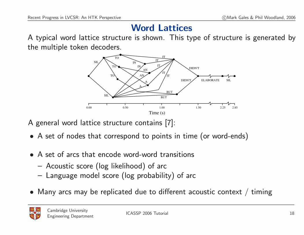
Word LatticesA typical word lattice structure is shown. This type of structure is generated bythe multiple token decoders.

SIL

SIL

TO

TO

TO

ITIT

IT

ITIT

INAN

AN

AA

BUT

BUT

DIDN'T

DIDN'T

ELABORATE SIL

IN

Time (s)0.00 0.50 1.00 1.50 2.25 2.85

A general word lattice structure contains [7]:

• A set of nodes that correspond to points in time (or word-ends)

• A set of arcs that encode word-word transitions

– Acoustic score (log likelihood) of arc– Language model score (log probability) of arc

• Many arcs may be replicated due to different acoustic context / timing




Some Lattice OperationsMost of these lattice operations are implemented in HLRescore

• Acoustic Recsoring

– Reduce lattice to word-graph with LM probs– Re-run recogniser with word-graph as language model but new acoustic

models– Often produce lattice output (for further processing)– Use HVite or HDecode

• LM Recsoring

– Expand lattice with new LM scores e.g. bigram to 4-gram– Re-compute 1-best word hypothesis

• Lattice Quality [7]

– Include all close alternatives to 1-best hypothesis– Aim to include correct answer




– Trade-off between size and coverage– Measure oracle lattice word error rate– Measure lattice density in arcs / second

• Pruning [7]

– Calulate the likelihood difference between most likely path that goes througha particular arc and overall lattice likelihood

– Prune out all arcs/nodes greater than a threshold away– Use complete sentence likelihoods (via lattice foward-backward)– Dramatically reduce lattice size with small effect on quality

• System Optimisation

– Vary grammar-scale factor / word-insertion penalty– Find 1-best from lattice with particular settings– Fast to tune these parameters




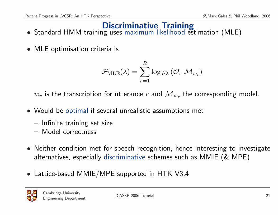
Discriminative Training• Standard HMM training uses maximum likelihood estimation (MLE)

• MLE optimisation criteria is

FMLE(λ) =R∑

r=1

log pλ (Or|Mwr)

wr is the transcription for utterance r and Mwr the corresponding model.

• Would be optimal if several unrealistic assumptions met

– Infinite training set size– Model correctness

• Neither condition met for speech recognition, hence interesting to investigatealternatives, especially discriminative schemes such as MMIE (& MPE)

• Lattice-based MMIE/MPE supported in HTK V3.4




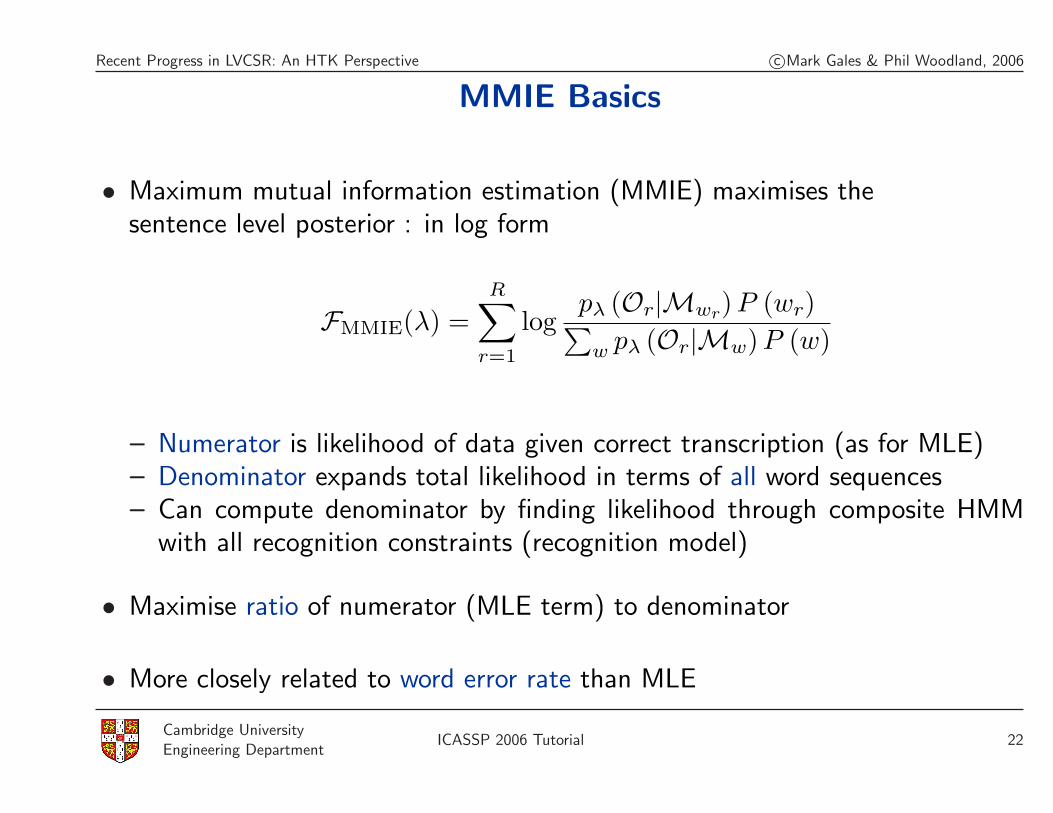
MMIE Basics

• Maximum mutual information estimation (MMIE) maximises thesentence level posterior : in log form

FMMIE(λ) =R∑

r=1

logpλ (Or|Mwr)P (wr)∑

w pλ (Or|Mw)P (w)

– Numerator is likelihood of data given correct transcription (as for MLE)– Denominator expands total likelihood in terms of all word sequences– Can compute denominator by finding likelihood through composite HMM

with all recognition constraints (recognition model)

• Maximise ratio of numerator (MLE term) to denominator

• More closely related to word error rate than MLE




• Strictly Conditional Maximum Likelihood Estimator

– but here MMI since LM fixed

• MMIE weights training data unequally (well classified small weight)

– MLE gives all training samples equal weight

• Sensitive to outliers

– Use of an error measure instead of MMIE would reduce sensitivity

• Simple example shows usefulness with incorrect model assumptions.

– Two class static pattern recognition problem– Two dimensional data from full covariance Gaussian– Modelled with diagonal covariance Gaussian




Simple MMIE Example

−4 −2 0 2 4 6 8−1

−0.5

0

0.5

1

1.5

2

2.5

3MLE SOLUTION (FULL−COVARIANCE)

−4 −2 0 2 4 6 8−1

−0.5

0

0.5

1

1.5

2

2.5

3MLE SOLUTION (DIAGONAL)

−4 −2 0 2 4 6 8−1

−0.5

0

0.5

1

1.5

2

2.5

3MMIE SOLUTION

1 2 3 4 5 6 7 8 9 10−1.1

−1

−0.9

−0.8

−0.7

−0.6

ITERATION

MMIE CRITERION / ERROR RATE

1 2 3 4 5 6 7 8 9 1010

15

20

25

30




MMIE Issues for LVCSR

• Need to have effective optimisation technique that scales well to large systems.

• Optimisation: Extended Baum-Welch [9, 10]

µjm =

{θnum

jm (O)− θdenjm (O)

}+ Dµjm{

γnumjm − γden

jm

}+ D

σ2jm =

{θnum

jm (O2)− θdenjm (O2)

}+ D(σ2

jm + µ2jm){

γnumjm − γden

jm

}+ D

− µ2jm

– Gaussian occupancies (summed over time) are γjm.– θjm(O) and θjm(O2) are sums of data and squared data respectively,

weighted by occupancy.– num and den denote correct word sequence, & recognition model

respectively.




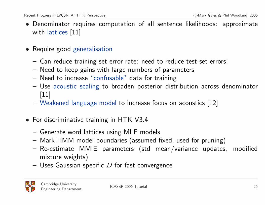
• Denominator requires computation of all sentence likelihoods: approximatewith lattices [11]

• Require good generalisation

– Can reduce training set error rate: need to reduce test-set errors!– Need to keep gains with large numbers of parameters– Need to increase “confusable” data for training– Use acoustic scaling to broaden posterior distribution across denominator

[11]– Weakened language model to increase focus on acoustics [12]

• For discriminative training in HTK V3.4

– Generate word lattices using MLE models– Mark HMM model boundaries (assumed fixed, used for pruning)– Re-estimate MMIE parameters (std mean/variance updates, modified

mixture weights)– Uses Gaussian-specific D for fast convergence




MPE Objective Function

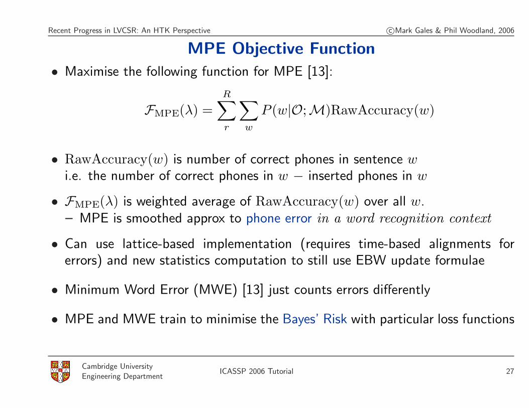
• Maximise the following function for MPE [13]:

FMPE(λ) =R∑r

∑w

P (w|O;M)RawAccuracy(w)

• RawAccuracy(w) is number of correct phones in sentence wi.e. the number of correct phones in w − inserted phones in w

• FMPE(λ) is weighted average of RawAccuracy(w) over all w.– MPE is smoothed approx to phone error in a word recognition context

• Can use lattice-based implementation (requires time-based alignments forerrors) and new statistics computation to still use EBW update formulae

• Minimum Word Error (MWE) [13] just counts errors differently

• MPE and MWE train to minimise the Bayes’ Risk with particular loss functions




Improved Generalisation using I-smoothing

• Use of discriminative criteria can easily cause over-training

• Get smoothed estimates of parameters by combining Maximum Likelihood(ML) and MPE objective functions for each Gaussian

• Rather than globally interpolate (H-criterion), amount of ML smoothingdepends on the amount of data per Gaussian

• I-smoothing adds τ samples of the average ML statistics for each Gaussian.Typically τ =50.

– For MMI scale numerator counts appropriately– For MPE need ML counts in addition to other MPE statistics

• I-smoothing essential for MPE (& helps a little for MMI)




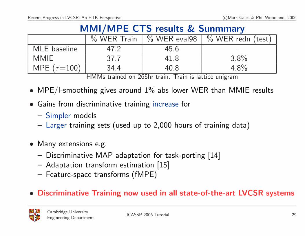
MMI/MPE CTS results & Sunmmary% WER Train % WER eval98 % WER redn (test)

MLE baseline 47.2 45.6 –MMIE 37.7 41.8 3.8%MPE (τ=100) 34.4 40.8 4.8%

HMMs trained on 265hr train. Train is lattice unigram

• MPE/I-smoothing gives around 1% abs lower WER than MMIE results

• Gains from discriminative training increase for

– Simpler models– Larger training sets (used up to 2,000 hours of training data)

• Many extensions e.g.

– Discriminative MAP adaptation for task-porting [14]– Adaptation transform estimation [15]– Feature-space transforms (fMPE)

• Discriminative Training now used in all state-of-the-art LVCSR systems




Speaker Adaptation and Adaptive Training

• Speaker/environment adaptation is an essential part of LVCSR systems

– obtain the performance of a Speaker/Environment dependent systemwith orders-of-magnitude less data (30 seconds vs 2000 hours!)

• The mode of adaptation depends on the task being investigated

– incremental: results are required causally, the adaptation data is not allavailable in one block - dictation tasks, car navigation

– batch: all the data is available (or can be used) in one block - BNtranscription, CTS transcription

In addition for batch adaptation the adaptation data may be

– supervised: the correct transcription of the adaptation data is known(dictation enrolment)

– unsupervised: no transcribed adaptation data available, transcription mustbe hypothesised (BN transcription)




General Adaptation Process

• Aim: Modify a “canonical” model to represent a target speaker

– transformation should require minimal data from the target speaker– adapted model should accurately represent target speaker

Adapt

Canonical Speaker Model Target Speaker Model

• Need to determine

– nature (and complexity) of the speaker transform– how to train the “canonical” model that is adapted




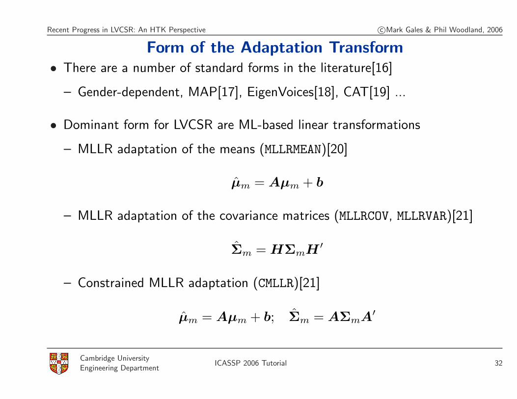
Form of the Adaptation Transform• There are a number of standard forms in the literature[16]

– Gender-dependent, MAP[17], EigenVoices[18], CAT[19] ...

• Dominant form for LVCSR are ML-based linear transformations

– MLLR adaptation of the means (MLLRMEAN)[20]

µm = Aµm + b

– MLLR adaptation of the covariance matrices (MLLRCOV, MLLRVAR)[21]

Σm = HΣmH ′

– Constrained MLLR adaptation (CMLLR)[21]

µm = Aµm + b; Σm = AΣmA′




Linear Transformation Estimation

• Estimation of all the transforms is based on EM[21]:

– requires the transcription/hypothesis of the adaptation data– iterative process using “current” transform to estimate new transform

TransformEstimate

Speaker Transform

Update CompleteData Set

Identity Transform

Adaptation DataRecognise

Statistics

Hypothesis

Transform

• Two iterative loops for estimation:

1. estimate hypothesis given transform2. update complete-dataset given

transform and hypothesis

referred to as Iterative MLLR[22]

• For supervised training hypothesis is known

• Can also vary complexity of transform withiteration




Adaptation Transform Complexity

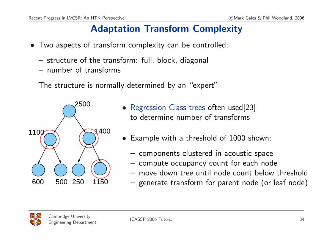
• Two aspects of transform complexity can be controlled:

– structure of the transform: full, block, diagonal– number of transforms

The structure is normally determined by an “expert”

2500

1400

1150600 500

1100

250

• Regression Class trees often used[23]to determine number of transforms

• Example with a threshold of 1000 shown:

– components clustered in acoustic space– compute occupancy count for each node– move down tree until node count below threshold– generate transform for parent node (or leaf node)




Lattice-Based MLLR

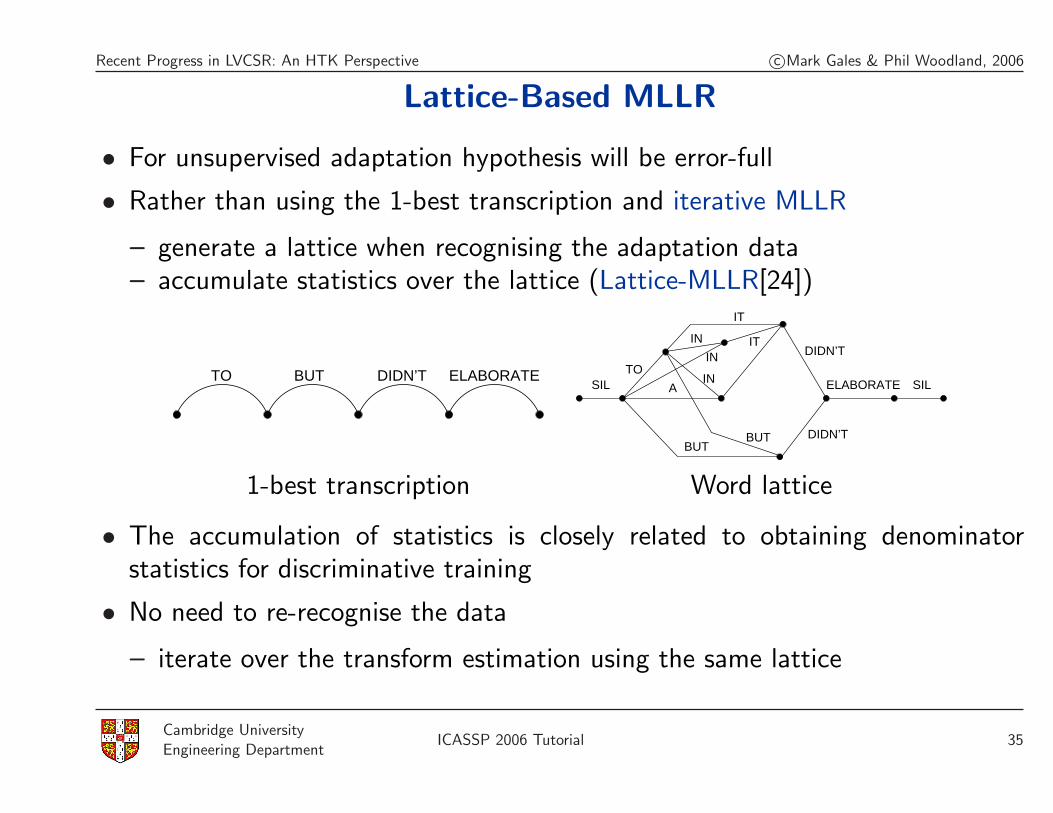
• For unsupervised adaptation hypothesis will be error-full

• Rather than using the 1-best transcription and iterative MLLR

– generate a lattice when recognising the adaptation data– accumulate statistics over the lattice (Lattice-MLLR[24])

DIDN’T ELABORATEBUTTOASIL SILELABORATE

DIDN’T

DIDN’TBUT

IN

IN

IN

TO

IT

IT

BUT

1-best transcription Word lattice

• The accumulation of statistics is closely related to obtaining denominatorstatistics for discriminative training

• No need to re-recognise the data

– iterate over the transform estimation using the same lattice




Training a “Good” Canonical Model

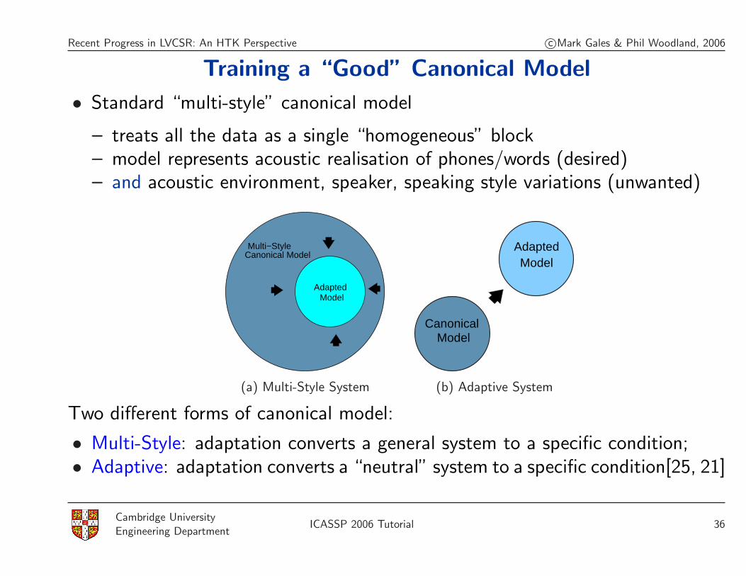
• Standard “multi-style” canonical model

– treats all the data as a single “homogeneous” block– model represents acoustic realisation of phones/words (desired)– and acoustic environment, speaker, speaking style variations (unwanted)

Multi−Style

ModelAdapted

Canonical Model

(a) Multi-Style System

AdaptedModel

Canonical Model

(b) Adaptive System

Two different forms of canonical model:

• Multi-Style: adaptation converts a general system to a specific condition;• Adaptive: adaptation converts a “neutral” system to a specific condition[25, 21]




Adaptive Training

TransformSpeaker 1 Speaker 1

ModelSpeaker 1

Data

CanonicalModel

TransformSpeaker 2 Speaker 2

Model

TransformSpeaker S Speaker S

Model

Speaker 2Data

Speaker SData

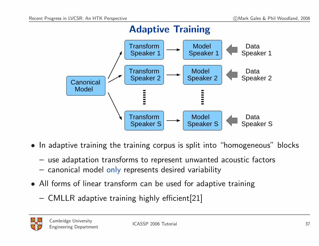
• In adaptive training the training corpus is split into “homogeneous” blocks

– use adaptation transforms to represent unwanted acoustic factors– canonical model only represents desired variability

• All forms of linear transform can be used for adaptive training

– CMLLR adaptive training highly efficient[21]




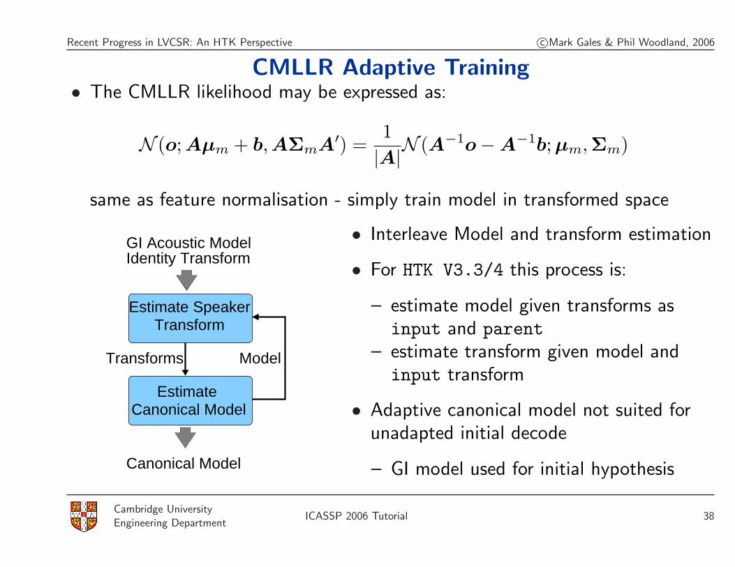
CMLLR Adaptive Training• The CMLLR likelihood may be expressed as:

N (o; Aµm + b, AΣmA′) =1|A|N (A−1o−A−1b; µm,Σm)

same as feature normalisation - simply train model in transformed space

Estimate SpeakerTransform

Canonical ModelEstimate

Transforms

Canonical Model

Model

GI Acoustic ModelIdentity Transform

• Interleave Model and transform estimation

• For HTK V3.3/4 this process is:

– estimate model given transforms asinput and parent

– estimate transform given model andinput transform

• Adaptive canonical model not suited forunadapted initial decode

– GI model used for initial hypothesis




Adaptation/Adaptive Training Summary

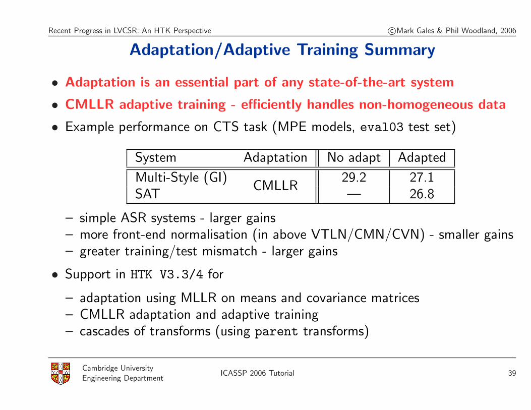
• Adaptation is an essential part of any state-of-the-art system

• CMLLR adaptive training - efficiently handles non-homogeneous data

• Example performance on CTS task (MPE models, eval03 test set)

System Adaptation No adapt Adapted

Multi-Style (GI)CMLLR

29.2 27.1SAT — 26.8

– simple ASR systems - larger gains– more front-end normalisation (in above VTLN/CMN/CVN) - smaller gains– greater training/test mismatch - larger gains

• Support in HTK V3.3/4 for

– adaptation using MLLR on means and covariance matrices– CMLLR adaptation and adaptive training– cascades of transforms (using parent transforms)




Structured Covariance Matrix Modelling

• State output distribution normally modelled using a GMM

bj(ot) =M∑

m=1

cjmN (ot; µjm,Σjm)

• Covariance matrix is normally assumed to be diagonal

– limits number of model parameters (O(d) rather than O(d2))– but assumes that elements of the feature vector uncorrelated

• Various forms of structured covariance matrices have been proposed

– factor-analysed HMMs[26], STC[27], SPAM[28], EMLLT[29] ...– precision-matrix (inverse covariance) models are popular due to efficiency




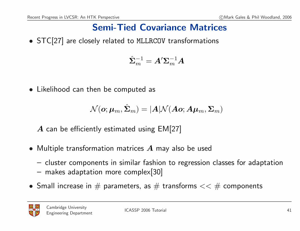
Semi-Tied Covariance Matrices

• STC[27] are closely related to MLLRCOV transformations

Σ−1m = A′Σ−1

m A

• Likelihood can then be computed as

N (o; µm, Σm) = |A|N (Ao; Aµm,Σm)

A can be efficiently estimated using EM[27]

• Multiple transformation matrices A may also be used

– cluster components in similar fashion to regression classes for adaptation– makes adaptation more complex[30]

• Small increase in # parameters, as # transforms << # components




Basis Superposition• A general framework for precision matrix modelling:

– component-specific basis interpolation weights λm

– P global symmetric basis matrices: S(1), . . . , S(P )

• Precision matrix modelled as

Σ−1m =

P∑

i=1

λmiS(i)

• General ML and MPE update formulae can be derived[31]

• STC can be written as

Σ−1m =

P∑

i=1

1σ2

mi

ai1...

aid

[

ai1 . . . aid

]

can also describe SPAM, EMLLT




Heteroscedastic LDA

• HLDA[32] is related to LDA and STC

– LDA without the constraint that all within-class covariances are the same– STC with additional sub-vector tying of the means and variances

• HLDA estimated using ML in same fashion as STC except constrain[27]

Aµm =[

µm[p]

µ

], Σm =

[Σm[p] 0

0 Σ

], A =

[A[p]

A[d−p]

]

d− p dimensional parameters µ and Σ tied over all components

• Likelihood calculated as

|A|N (Ao; Aµm,Σm) =(|A|N (A[p]o; µm[p],Σm[p])

)N (A[d−p]o; µ,Σ)

– as the final d− p dimensions are all tied, no discrimination– effectively projected from d → p dimensions




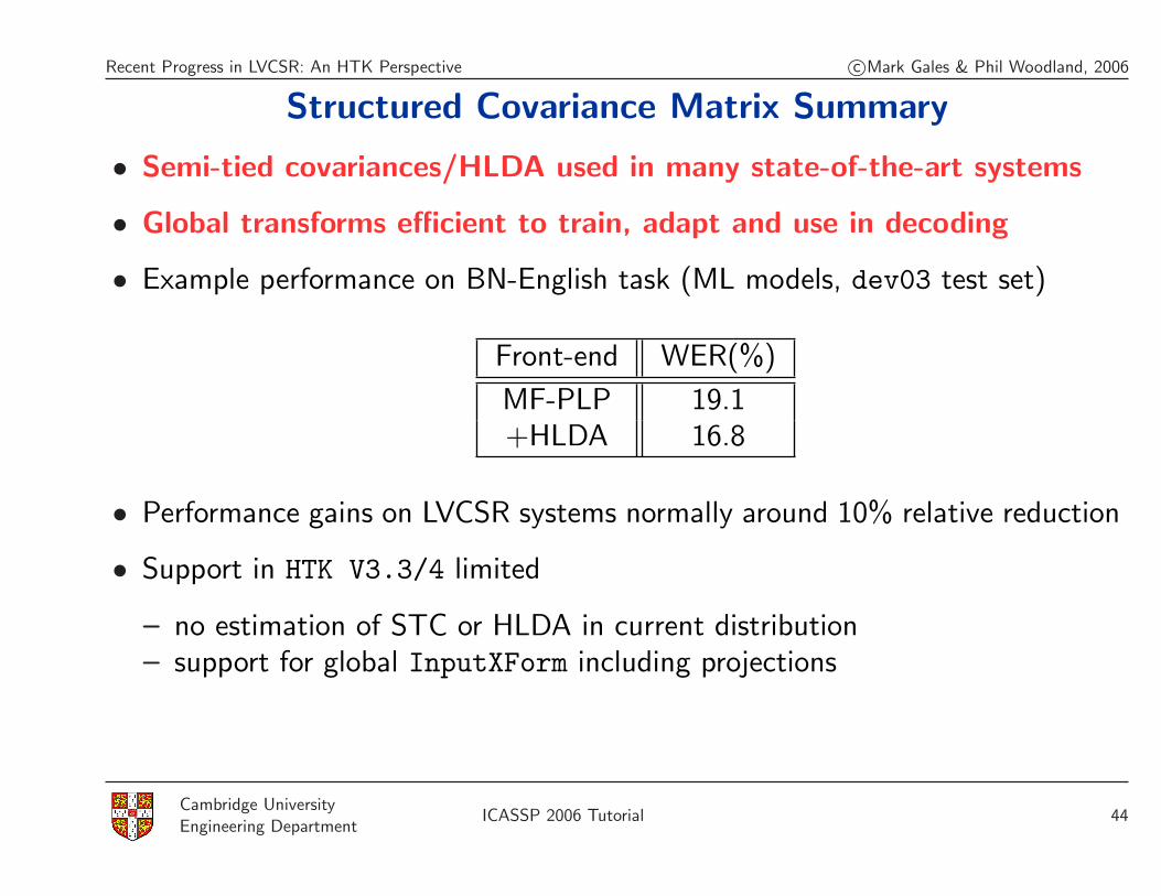
Structured Covariance Matrix Summary

• Semi-tied covariances/HLDA used in many state-of-the-art systems

• Global transforms efficient to train, adapt and use in decoding

• Example performance on BN-English task (ML models, dev03 test set)

Front-end WER(%)

MF-PLP 19.1+HLDA 16.8

• Performance gains on LVCSR systems normally around 10% relative reduction

• Support in HTK V3.3/4 limited

– no estimation of STC or HLDA in current distribution– support for global InputXForm including projections




Found Data and Closed Captions

• There is a vast quantity of found audio data

– radio, television, podcasts etc– but expensive to produce manual transcriptions (takes 5-10 times RT)

• USA - FCC requires that 95% of new TV programs include Closed Captions

– accurate transcriptions typically include:exact word level transcription, non-speech events, speaker id

– CC transcriptions typically reflect the meaning, but typicallyhesitations/repetitions not marked, possible word order changes

– NIST found level of disagreement of the order of 12%

Can these rough CC be used to train an ASR system?How to select appropriate audio data for training?

• Current approaches use the closed caption to generate a biased LM[33, 34, 35]




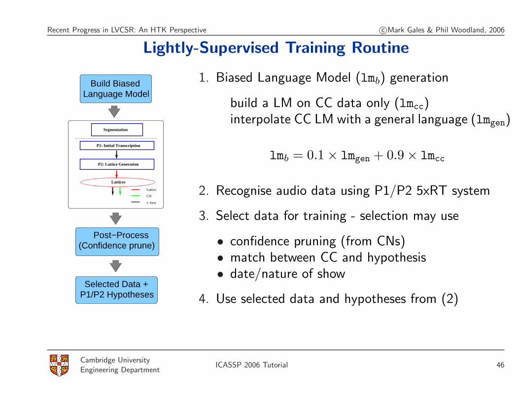
Lightly-Supervised Training Routine



Lattices

1−best

CN

Lattice

(Confidence prune)Post−Process

P1/P2 HypothesesSelected Data +

Language ModelBuild Biased

Segmentation

1. Biased Language Model (lmb) generation

build a LM on CC data only (lmcc)interpolate CC LM with a general language (lmgen)

lmb = 0.1× lmgen + 0.9× lmcc

2. Recognise audio data using P1/P2 5xRT system

3. Select data for training - selection may use

• confidence pruning (from CNs)• match between CC and hypothesis• date/nature of show

4. Use selected data and hypotheses from (2)




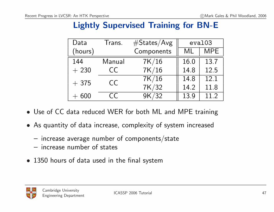
Lightly Supervised Training for BN-E

Data Trans. #States/Avg eval03(hours) Components ML MPE

144 Manual 7K/16 16.0 13.7+ 230 CC 7K/16 14.8 12.5

+ 375 CC7K/16 14.8 12.17K/32 14.2 11.8

+ 600 CC 9K/32 13.9 11.2

• Use of CC data reduced WER for both ML and MPE training

• As quantity of data increase, complexity of system increased

– increase average number of components/state– increase number of states

• 1350 hours of data used in the final system




Found Data and Closed-Captions Summary

• Large quantities of “found” data available for “free”

• High quality transcriptions normally not available

– closed captions (and related) are available for many sources– these CC and related transcriptions may be used for training system

• Large performance gains obtained using large quantities of CC data

• How to rapidly select data from the possible sources an open question

– normally build a system on various subsets and test performance ondevelopment data




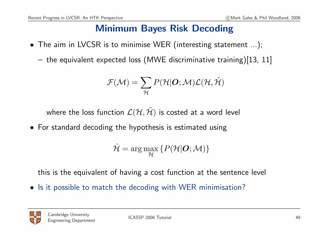
Minimum Bayes Risk Decoding

• The aim in LVCSR is to minimise WER (interesting statement ...);

– the equivalent expected loss (MWE discriminative training)[13, 11]

F(M) =∑

HP (H|O;M)L(H, H)

where the loss function L(H, H) is costed at a word level

• For standard decoding the hypothesis is estimated using

H = arg maxH

{P (H|O;M)}

this is the equivalent of having a cost function at the sentence level

• Is it possible to match the decoding with WER minimisation?




Confusion Network Decoding• If the confusions could be split at the word level, could use:

H =L∑

i=1

arg maxW(i)

{P (W(i)|O;M)

}

this should minimise the WER rather than sentence error rate.

ASIL SILELABORATE

DIDN’T

DIDN’TBUT

IN

IN

IN

TO

IT

IT

BUT

TO IN DIDN’TIT ELABORATE

!NULLA

BUT

!NULL

!NULL

Word lattice Confusion Network

• Confusion networks[36] are one approach to this

– use standard HMM decoder to generate word lattice;– iteratively merge links to form confusion networks (CN) from word lattice.




Complementary System Generation/Combination

• It is hard to produce a single system that performs well on all data

• A standard machine learning approach is to build multiple, complementary,systems (e.g. ADABoost)

How to build/select systems that are complementary?How to combine multiple systems together?

• Building explicitly complementary systems is still an open question, currently

– build many diverse systems - tri/quin-phone, MFCC/PLP, SAT/GD/GI– try combinations and pick the best

Not elegant, but it works! Diversity of models is important

• Range of options for combining systems:

– cross-adaptation: hypothesis from one system used to adapt another[37]– explicitly combine the individual system hypotheses




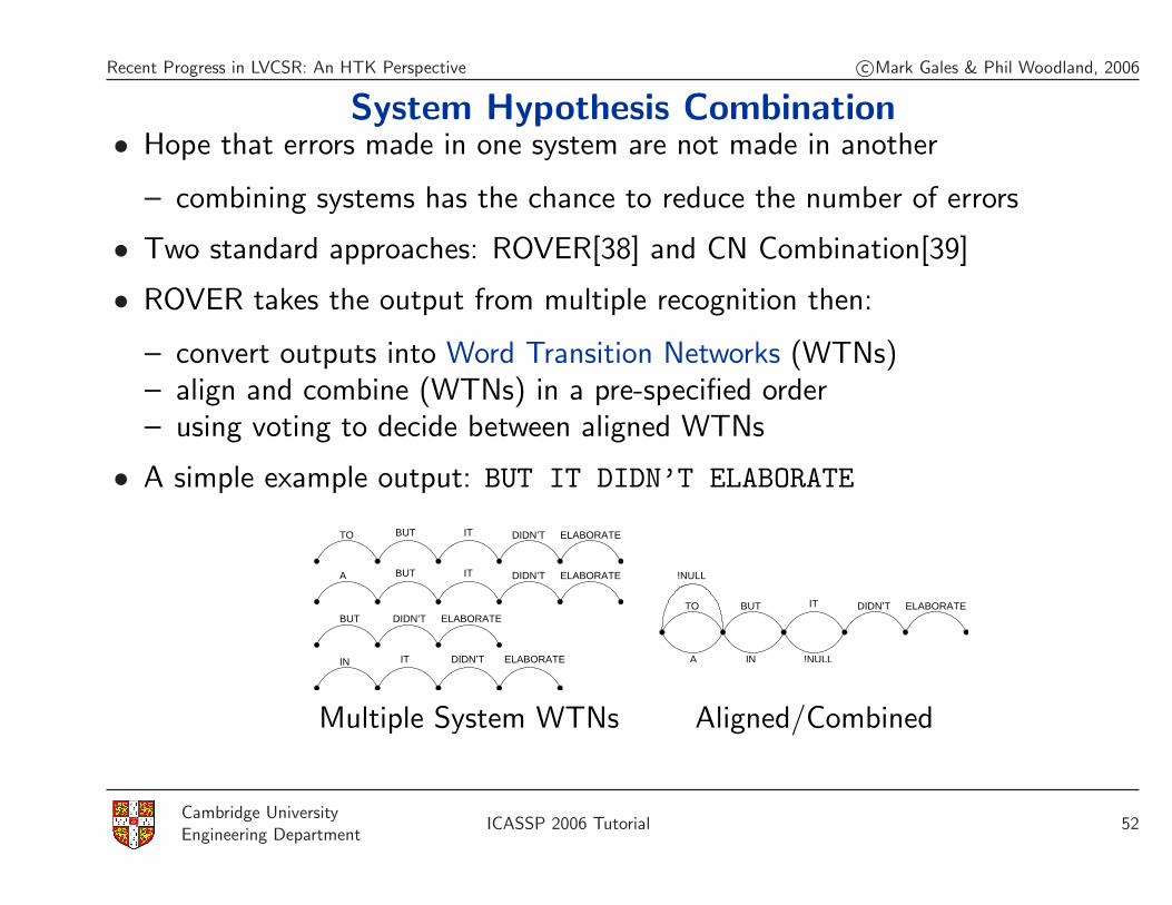
System Hypothesis Combination• Hope that errors made in one system are not made in another

– combining systems has the chance to reduce the number of errors

• Two standard approaches: ROVER[38] and CN Combination[39]

• ROVER takes the output from multiple recognition then:

– convert outputs into Word Transition Networks (WTNs)– align and combine (WTNs) in a pre-specified order– using voting to decide between aligned WTNs

• A simple example output: BUT IT DIDN’T ELABORATE

TO DIDN’TIT ELABORATEBUT

A DIDN’TIT ELABORATEBUT

BUT

IN

DIDN’T ELABORATE

IT DIDN’T ELABORATE

TO DIDN’TIT ELABORATE

!NULLA

!NULL

IN

BUT

Multiple System WTNs Aligned/Combined




Confusion Network Combination

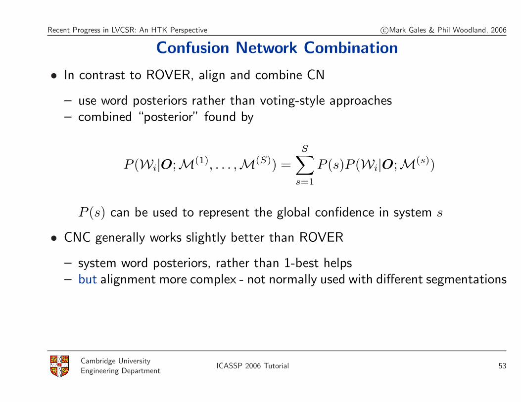
• In contrast to ROVER, align and combine CN

– use word posteriors rather than voting-style approaches– combined “posterior” found by

P (Wi|O;M(1), . . . ,M(S)) =S∑

s=1

P (s)P (Wi|O;M(s))

P (s) can be used to represent the global confidence in system s

• CNC generally works slightly better than ROVER

– system word posteriors, rather than 1-best helps– but alignment more complex - not normally used with different segmentations




Confusion Networks and System Combination Summary

• Standard (Viterbi) decoding minimises sentence-level loss

• Confusion networks: an approach to minimising word-level loss

– Example performance on CTS task (ML models, eval04 test set)

Decoding WER(%) SER(%)

Viterbi 29.9 32.9CN 29.2 33.1

– reduces WER, increases Sentence Error Rate (SER)– gains in WER varies (normally reduced when adaptation is used)

• System combination is used in most state-of-the-art systems

– system combined either using ROVER or CNC– Performance gains depend on systems making different errors

• No confusion network support in HTK V3.4 currently




CU-HTK Multi-Pass/Combination Framework


Adapt

P3x

Lattices

Adapt

P3a


Segmentation

Alignment

CNC

1−best

CN

Lattice

• P1 used to generate initial hypothesis

• P1 hypothesis used for rapid adaptation

– LSLR, diagonal variance transforms

• P2: lattices generated for rescoring

– apply complex LMs to trigram lattices

• P3 Adaptation

– 1-best CMLLR– Lattice-based MLLR– Lattice-based full variance

• CN Decoding/Combination

• Segmentation/P1-P2 branches runs in < 5xRT, full configuration < 10xRT.




General CU-HTK System Description

• Front-end:

– base front-end 12 MF-PLP plus normalised log-energy (13 dim)– segment-level Cepstral Mean Normalisation (CMN)– delta, delta-delta, delta-delta-delta appended (52 dim)– HLDA projection 52 → 39 dimensions

• Acoustic Models:

– state-clustered decision tree tri-phone models– Gender-Independent (GI) models– Gender Dependent (GD) models - male/female component variances tied– GMM used for state-output distributions– all models MPE trained

• Language Models:

– generate separate tri-gram, four-grams, class-based N-grams on sources– interpolate sources to minimise perplexity on development data




English Broadcast News System Description

• Segmentation and clustering:

– LIMSI kindly supplied segmentation and clustering


– 1350 hours of data (144hrs manual transcriptions)

• Language Models:

– 928MWords of text split into 5 language models and interpolated– word and class-based four-gram LMs used in P2 lattice rescoring

• P3 Branch models:

– GD multiple pron. dictionary model (P3b GD-MPron) - contrast for P2– GD single pronunciation dictionary model[40] (P3c GD-SPron)– SAT multiple pronunciation dictionary model (P3a SAT-MPron)

• For more details see[41]




English Broadcast News Transcription

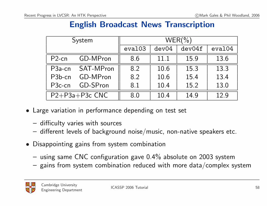
System WER(%)eval03 dev04 dev04f eval04

P2-cn GD-MPron 8.6 11.1 15.9 13.6

P3a-cn SAT-MPron 8.2 10.6 15.3 13.3P3b-cn GD-MPron 8.2 10.6 15.4 13.4P3c-cn GD-SPron 8.1 10.4 15.2 13.0

P2+P3a+P3c CNC 8.0 10.4 14.9 12.9

• Large variation in performance depending on test set

– difficulty varies with sources– different levels of background noise/music, non-native speakers etc.

• Disappointing gains from system combination

– using same CNC configuration gave 0.4% absolute on 2003 system– gains from system combination reduced with more data/complex system




Mandarin Broadcast News System Description• Mandarin specific features (full description in[42] - see ICASSP poster)

• Front-end:

– pitch (plus delta, delta-delta) added after HLDA– optional GMM-based Gaussianisation[43] applied


– tonal questions added to the set of decision-tree questions.– 148 hours of Mandarin, 11 hours of English (dual language system)

• Language Models;

– best-first search for character-to-word segmentation– about 400M “Words” of text data - word trigram only


– GD HLDA front-end system (P3b GD-HLDA) - contrast for P2– GD Gaussianised HLDA front-end system (P3d GD-GAUSS)– SAT Gaussianised HLDA front-end system (P3e SAT-GAUSS)




Mandarin Broadcast News Transcription

System CER (%)eval04

P2-cn GD-HLDA 17.6

P3b-cn GD-HLDA 17.0P3d-cn GD-GAUSS 16.6P3e-cn SAT-GAUSS 16.4

P3e+P3d CNC 16.3

• Recognition performance measured in Character Error Rate (CER)

• Use of P2 in CNC stage did not help

• Gaussianisation (GAUSS) helped over standard HLDA front-end

– additional normalisation helps when using smaller training sets– SAT gave small further gains over GAUSS

• CNC gave only small gains




English Conversational Telephone Speech Description

• Task-specific modifications to general system (full description in[44])

• Front-end:

– Vocal Tract Length Normalisation (VTLN) applied– Cepstral Variance Normalisation (CVN) applied (Jacobian normalisation)

• Acoustic model training data:

– about 2300 hours of data, quinphone and triphone models built

• Language model training data:

– 1,000MWords of text split into 6 language models and interpolated– word and class-based four-gram LMs used in P2 lattice rescoring


– GD multiple pronunciation dictionary model (P3b GD-MPron)– quinphone SAT single pron. dictionary model (P3e SAT-SPron-Quin)




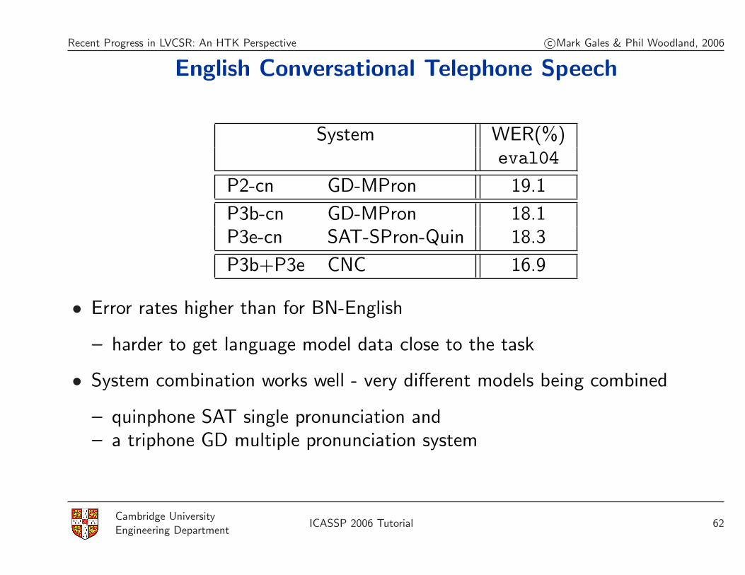
English Conversational Telephone Speech

System WER(%)eval04

P2-cn GD-MPron 19.1

P3b-cn GD-MPron 18.1P3e-cn SAT-SPron-Quin 18.3

P3b+P3e CNC 16.9

• Error rates higher than for BN-English

– harder to get language model data close to the task

• System combination works well - very different models being combined

– quinphone SAT single pronunciation and– a triphone GD multiple pronunciation system




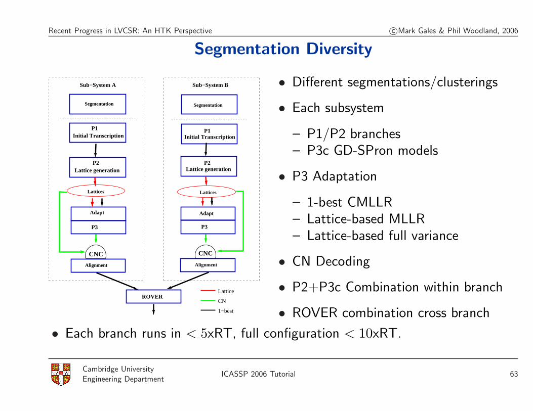
Segmentation Diversity

Lattices

P3P3

Lattice generationP2

P1P1

P2

Initial Transcription

Lattice generation

Initial Transcription

Adapt

Lattices

Adapt

AlignmentAlignment

ROVER

CNCCNC

Segmentation Segmentation

Sub−System BSub−System A

1−best

CN

Lattice

• Different segmentations/clusterings

• Each subsystem

– P1/P2 branches– P3c GD-SPron models

• P3 Adaptation

– 1-best CMLLR– Lattice-based MLLR– Lattice-based full variance

• CN Decoding

• P2+P3c Combination within branch

• ROVER combination cross branch

• Each branch runs in < 5xRT, full configuration < 10xRT.




Segmentation Diversity BN-English Results

System Segment/ WER(%)Clustering eval04

L0+P3c LIMSICNC

12.8B0+P3c BBN 13.0C0+P3c CU 13.3

L0+P3c⊕ C0+P3cROVER

12.6L0+P3c⊕ B0+P3c 12.4

• Three segmentations and clusterings: CU, BBN and LIMSI (thanks to BBNand LIMSI)

– all segmentations/clusterings very different (CU deliberately very different)

• Diversity in segmentation gives gains in combination

– combining BBN and LIMSI 0.5% better than using general framework

• Framework used for the RT04f BN-English EARS evaluation




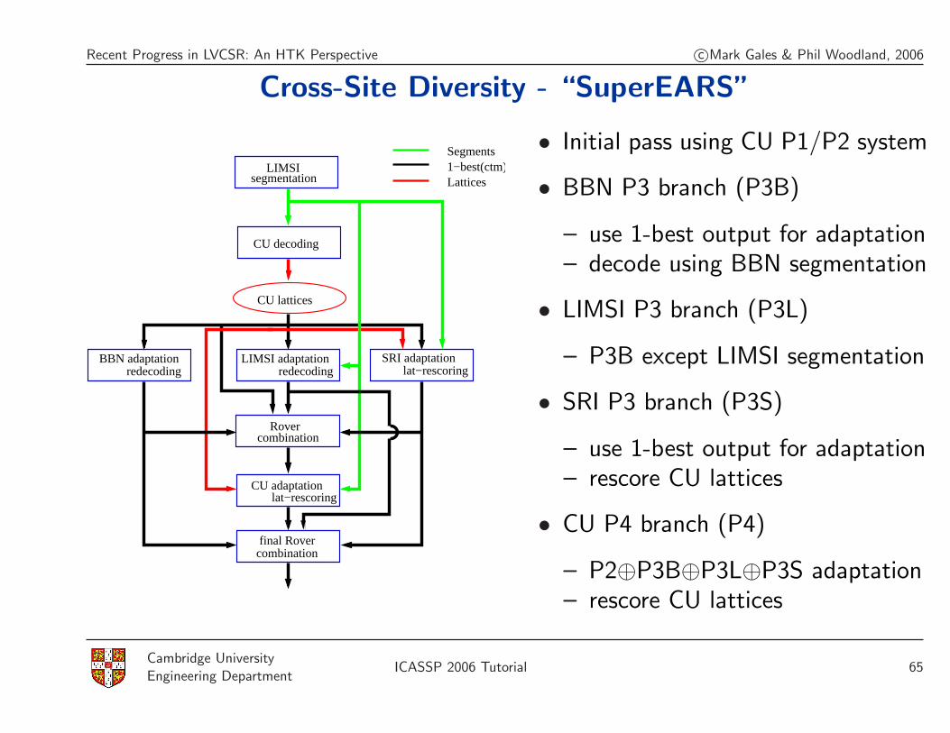
Cross-Site Diversity - “SuperEARS”

BBN adaptation

segmentationLIMSI

combinationRover

final Rovercombination

CU decoding

lat−rescoringCU adaptation

redecoding redecodingLIMSI adaptation SRI adaptation

lat−rescoring

CU lattices

Segments1−best(ctm)Lattices

• Initial pass using CU P1/P2 system

• BBN P3 branch (P3B)

– use 1-best output for adaptation– decode using BBN segmentation

• LIMSI P3 branch (P3L)

– P3B except LIMSI segmentation

• SRI P3 branch (P3S)

– use 1-best output for adaptation– rescore CU lattices

• CU P4 branch (P4)

– P2⊕P3B⊕P3L⊕P3S adaptation– rescore CU lattices




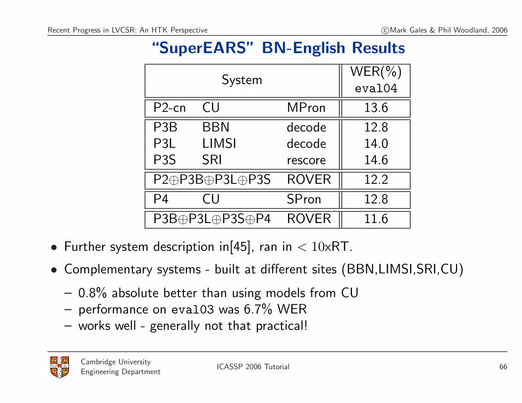
“SuperEARS” BN-English Results

SystemWER(%)eval04

P2-cn CU MPron 13.6

P3B BBN decode 12.8P3L LIMSI decode 14.0P3S SRI rescore 14.6

P2⊕P3B⊕P3L⊕P3S ROVER 12.2

P4 CU SPron 12.8

P3B⊕P3L⊕P3S⊕P4 ROVER 11.6

• Further system description in[45], ran in < 10xRT.

• Complementary systems - built at different sites (BBN,LIMSI,SRI,CU)

– 0.8% absolute better than using models from CU– performance on eval03 was 6.7% WER– works well - generally not that practical!




CU-HTK BN-English 1xRT System



Lattices

1−best

CN

Lattice

Alignment

Segmentation

0.16 0.18 0.2 0.22 0.24 0.2612

14

16

18

20

22

24

26

%W

ER

Pass1 running time (xRT)

Pass1Pass2

• Can use multi-pass framework for 1xRT systems (for details see[41])

– initial pass (P1) for adaptation supervision, adapted decode in P2

• Modified version of < 10xRT P1-P2 system

– P1: smaller acoustic and language models, heavily pruned search– P2: slightly smaller language model, pruned search

• Effect of P1 search vs WER% at P2 stage shown (dev04) - little effect




BN-English 1xRT Results

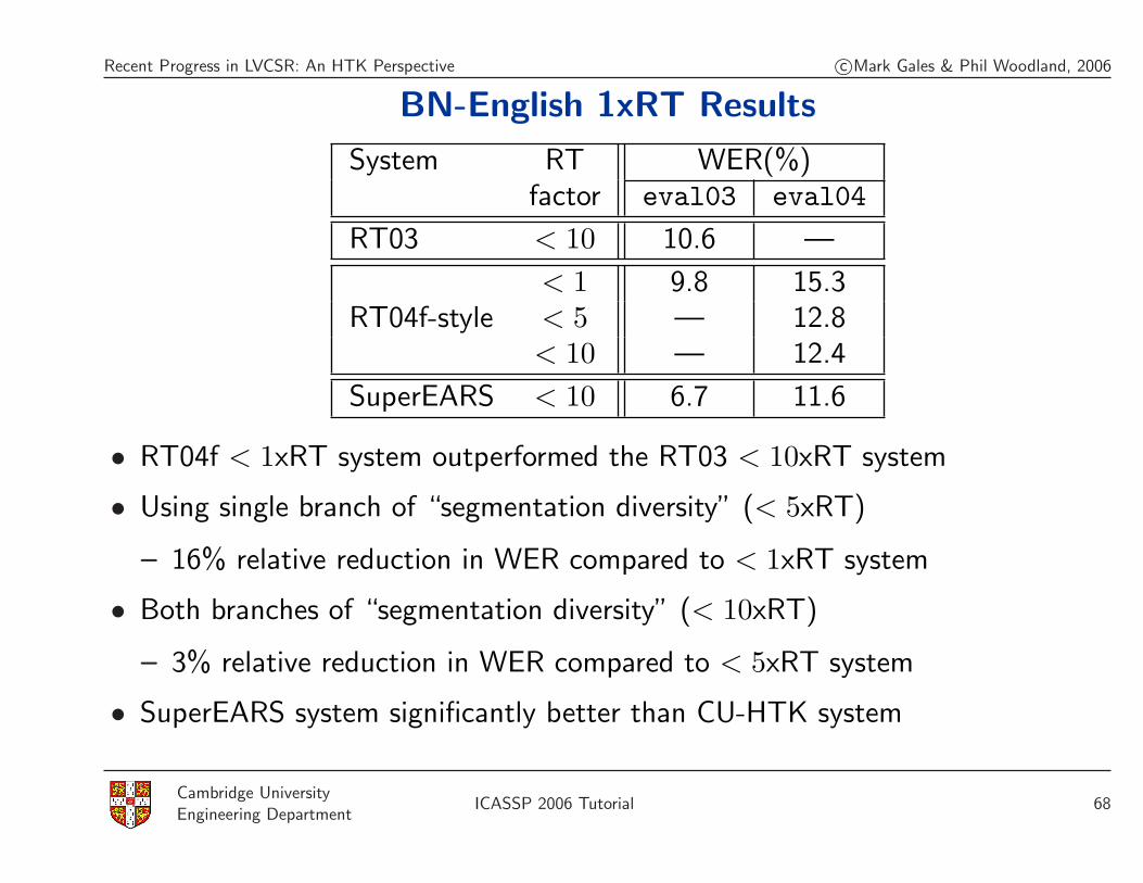
System RT WER(%)factor eval03 eval04

RT03 < 10 10.6 —

< 1 9.8 15.3RT04f-style < 5 — 12.8

< 10 — 12.4

SuperEARS < 10 6.7 11.6

• RT04f < 1xRT system outperformed the RT03 < 10xRT system

• Using single branch of “segmentation diversity” (< 5xRT)

– 16% relative reduction in WER compared to < 1xRT system

• Both branches of “segmentation diversity” (< 10xRT)

– 3% relative reduction in WER compared to < 5xRT system

• SuperEARS system significantly better than CU-HTK system




Summary

• Reviewed basic building blocks for speech recognition

• Described range of state-of-the-art techniques:

– discriminative training– adaptation and adaptive training– structured precision matrices– lightly supervised training– confusion network decoding and system combination

• Described CU-HTK multi-pass combination frameworks

– Languages: English and Mandarin– Tasks: Broadcast News and Conversation Telephone Speech transcription

LVCSR systems make use of large amounts of dataLVCSR systems are complex involving many techniques




References[1] S. J. Young, G. Evermann, M. J. F. Gales, T. Hain, D. Kershaw, G. Moore, J. Odell, D. Ollason, D. Povey, V. Valtchev, and P. C.

Woodland, The HTK Book, version 3.4. Cambridge, UK: Cambridge University Engineering Department, 2006.

[2] D. Y. Kim, S. Umesh, M. J. F. Gales, T. Hain, and P. C. Woodland, “Using VTLN for Broadcast News transcription,” in Proc. Int.Conf. Spoken Lang. Process., Jeju island, South Korea, October 2004.

[3] P. C. Woodland, “The development of the HTK Broadcast News transcription system: an overview,” Speech Communication, vol. 37,pp. 47–67, 2002.

[4] J.-L. Gauvain, L. Lamel, and G. Adda, “Partitioning and transcription of broadcast news data,” in Proc. Int. Conf. Spoken Lang.Process., vol. 4, Sydney, Australia, December 1998, pp. 1335–1338.

[5] S. J. Young, J. Odell, and P. C. Woodland, “Tree-based state tying for high accuracy acoustic modelling,” in Proc. ARPA HumanLanguage Technology Workshop, 1994.

[6] A. Stolcke, “SRILM – an extensible language modeling toolkit,” in Proc. Int. Conf. Spoken Lang. Process., Denver, CO, September2002.

[7] P. C. Woodland, C. J. Leggetter, J. J. Odell, V. Valtchev, and S. J. Young, “The 1994 HTK large vocabulary speech recognitionsystem,” in Proc. ICASSP, 1995.

[8] A. Stolcke, “Entropy-based pruning of backoff language models,” in Proc. DARPA News Transcription and Understanding Workshop,1998.

[9] P. Gopalakrishnan, D. Kanevsky, A. Nadas, and D. Nahamoo, “An inequality for rational functions with applications to some statisticalestimation problems,” IEEE Trans. Information Theory, 1991.

[10] Y. Normandin, “An improved MMIE training algorithm for speaker independent, small vocabulary, continuous speech recognition,” inProc. ICASSP, 1991.

[11] P. C. Woodland and D. Povey, “Large scale discriminative training of hidden Markov models for speech recognition,” Computer Speech& Language, vol. 16, pp. 25–47, 2002.

[12] R. Schluter, B. Muller, F. Wessel, and H. Ney, “Interdependence of language models and discriminative training,” in Proc. ASRU,1999.

[13] D. Povey and P. C. Woodland, “Minimum phone error and I-smoothing for improved discriminative training,” in Proc. IEEE Int. Conf.Acoust., Speech, Signal Process., Orlando, FL, May 2002.




[14] D. Povey, M. J. F. Gales, D. Y. Kim, and P. C. Woodland, “MMI-MAP and MPE-MAP for acoustic model adaptation,” in Proc. Eur.Conf. Speech Commun. Technol., Geneva, Switzerland, September 2003.

[15] L. Wang and P. Woodland, “Discriminative adaptive training using the MPE criterion,” in Proc. ASRU, 2003.

[16] P. C. Woodland, “Speaker adaptation for continuous density HMMs: A review,” in ISCA Adaptation Workshop., 2001.

[17] J. L. Gauvain and C.-H. Lee, “Maximum a-posteriori estimation for multivariate Gaussian mixture observations of Markov chains,”IEEE Transactions Speech and Audio Processing, vol. 2, pp. 291–298, 1994.

[18] R. Kuhn, P. Nguyen, J.-C. Junqua, L. Goldwasser, N. Niedzielski, S. Fincke, K. Field, and M. Contolini, “Eigenvoices for speakeradaptation,” in Proceedings ICSLP, 1998, pp. 1771–1774.

[19] M. J. F. Gales, “Cluster adaptive training of hidden Markov models,” IEEE Transactions Speech and Audio Processing, vol. 8, pp.417–428, 2000.

[20] C. J. Leggetter and P. C. Woodland, “Maximum likelihood linear regression for speaker adaptation of continuous density HMMs,”Computer Speech and Language, vol. 9, pp. 171–186, 1995.

[21] M. J. F. Gales, “Maximum likelihood linear transformations for HMM-based speech recognition,” Computer Speech and Language,vol. 12, pp. 75–98, 1998.

[22] P. C. Woodland, D. Pye, and M. J. F. Gales, “Iterative unsupervised adaptation using maximum likelihood linear regression,” in Proc.Int. Conf. Spoken Lang. Process., Philadelphia, 1996, pp. 1133–1136.

[23] C. J. Leggetter and P. C. Woodland, “Flexible speaker adaptation for large vocabulary speech recognition,” in Proceedings Eurospeech,1995, pp. 1155–1158.

[24] L. F. Uebel and P. C. Woodland, “Speaker adaptation using lattice-based MLLR,” in Proc. ITRW on Adaptation Methods for SpeechRecognition, 2001.

[25] T. Anastasakos, J. McDonough, R. Schwartz, and J. Makhoul, “A compact model for speaker-adaptive training,” in ProceedingsICSLP, 1996, pp. 1137–1140.

[26] A.-V. Rosti and M. J. F. Gales, “Factor analysed hidden Markov models for speech recognition,” Computer Speech and Language,2004.

[27] M. J. F. Gales, “Semi-tied covariance matrices for hidden Markov models,” IEEE Transactions Speech and Audio Processing, vol. 7,pp. 272–281, 1999.

[28] S. Axelrod, R. Gopinath, and P. Olsen, “Modeling with a subspace constraint on inverse covariance matrices,” in Proc. ICSLP, 2002.




[29] P. A. Olsen and R. A. Gopinath, “Modeling inverse covariance matrices by basis expansion,” in Proceedings ICASSP, 2002.

[30] K. C. Sim and M. J. F. Gales, “Adaptation of precision matric models on large vocabulary continuous speech recognition,” in ICASSP,2005.

[31] ——, “Minimum phone error training of precision matrix models,” IEEE Transactions Audio, Speech and Language Processing, 2006,to appear.

[32] N. Kumar, “Investigation of silicon-auditory models and generalization of linear discriminant analysis for improved speech recognition,”Ph.D. dissertation, John Hopkins University, 1997.

[33] L. Lamel and J.-L. Gauvain, “Lightly supervised and unsupervised acoustic model training,” Computer Speech and Language, vol. 16,pp. 115–129, 2002.

[34] H. Y. Chan and P. C. Woodland, “Improving broadcast news transcription by lightly supervised discriminative training,” in Proc. IEEEInt. Conf. Acoust., Speech, Signal Process., Montreal, Canada, March 2004.

[35] L. Nguyen and B. Xiang, “Light supervision in acoustic model training,” in Proc. IEEE Int. Conf. Acoust., Speech, Signal Process.,Montreal, Canada, March 2004.

[36] L. Mangu, E. Brill, and A. Stolcke, “Finding consensus among words: Lattice-based word error minimization,” in Proc. Eur. Conf.Speech Commun. Technol., 1999.

[37] L. Nguyen, S. Abdou, M. Afify, J. Makhoul, S. Matsoukas, R. Schwartz, B. Xiang, L. Lamel, J. Gauvain, G. Adda, H. Schwenk,and F. Lefevre, “The 2004 BBN/LIMSI 10xRT English Broadcast News transcription system,” in Proc. Fall 2004 Rich TranscriptionWorkshop (RT-04), Palisades, NY, November 2004.

[38] J. G. Fiscus, “A post-processing system to yield reduced word error rates: Recogniser Output Voting Error Reduction (ROVER),” inProc. IEEE ASRU Workshop, 1997.

[39] G. Evermann and P. C. Woodland, “Posterior probability decoding, confidence estimation and system combination,” in Proc. SpeechTranscription Workshop, College Park, MD, May 2000.

[40] T. Hain, “Implicit pronunciation modelling in ASR,” in ISCA ITRW PMLA, 2002.

[41] M. J. F. Gales, D. Kim, P. C. Woodland, H. Chan, D. Mrva, R. Sinha, and S. Tranter, “Progress in the CU-HTK Broadcast Newstranscription system,” IEEE Transactions Audio, Speech and Language Processing, 2006, to appear.

[42] R. Sinha, M. J. F. Gales, D. Kim, X. Liu, K. Sim, and P. C. Woodland, “The CU-HTK Broadcast News transcription system,” inProceedings ICASSP, 2006.




[43] M. J. F. Gales, B. Jia, X. Liu, K. C. Sim, P. C. Woodland, and K. Yu, “Development of the CUHTK 2004 Mandarin conversationaltelephone speech transcription system,” in Proc. IEEE Int. Conf. Acoust., Speech, Signal Process., Philadelphia, PA, March 2005.

[44] G. Evermann, H. Chan, M. J. F. Gales, B. Jia, X. Liu, D. Mrva, K. Sim, L. Wang, P. C. Woodland, and K. Yu, “Development of the2004 CU-HTK English CTS systems using more than two thousand hours of data,” in Proc. Fall 2004 Rich Transcription Workshop(RT-04f), 2004.

[45] P. C. Woodland, H. Y. Chan, G. Evermann, M. J. F. Gales, D. Y. Kim, X. A. Liu, D. Mrva, K. C. Sim, L. Wang, K. Yu, J. Makhoul,R. Schwartz, L. Nguyen, S. Matsoukas, B. Xiang, M. Afify, S. Abdou, J.-L. Gauvain, L. Lamel, H. Schwenk, G. Adda, F. Lefevre,D. Vergyri, W. Wang, J. Zheng, A. Venkataraman, R. R. Gadde, and A. Stolcke, “SuperEARS: Multi-site broadcast news system,” inProc. Fall 2004 Rich Transcription Workshop (RT-04), Palisades, NY, November 2004.



Documents

Recent Progress in Large Vocabulary Continuous Speech ...cs136a/CS136a_docs/HTK_icassp06_tutorial.pdf · Recent Progress in Large Vocabulary Continuous Speech Recognition: An HTK