Recent developments on computing PDFs using the quasi-PDF approach

Fernanda Steffens

DESY – Zeuthen

In collaboration with: Constantia Alexandrou (Univ. of Cyprus; Cyrpus Institute),Krzysztof Cichy (Goethe Uni. Frankfurt am Main; Adam Mickiewicz, PolandMartha Constantinou (Temple University)Kyriakos Hadjiyiannakou (Univ. of Cyrpus)Karl Jansen (DESY – Zeuthen)Haralambos Panagopoulos (Uni. Of Cyprus)Aurora Scapellato (HPC-LEAP; Uni. Of Cyprus; Uni. of Wuppertal)

Outline

• Introduction

• Quark distributions and quark quasi-distributions

• Extracting quark distributions from the quasi-distributions

• Lattice results for unrenormalized distributions

• Nonperturbative Renormalization I: RI-MOM scheme

Renormalized Matrix elements 𝑚𝜋 = 350 MeV

Renormalized matrix elements at the physical point

• Nonperturbative Renormalization II: The auxiliary field Approach

• Summary and outline

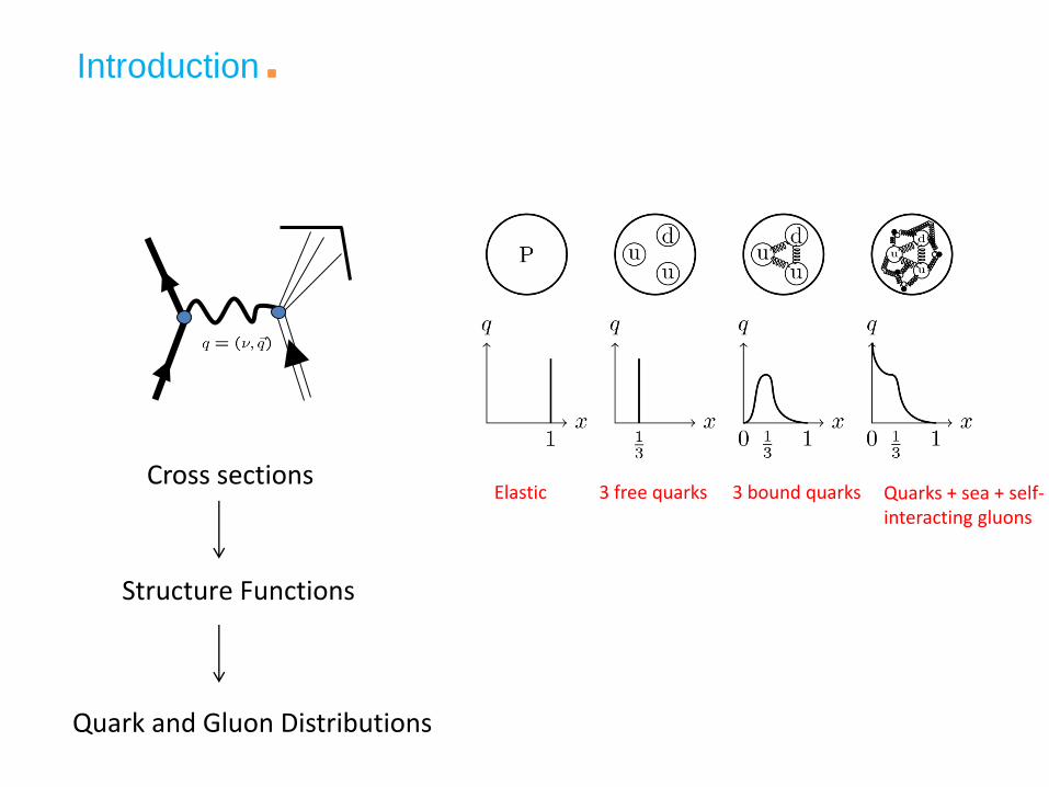
Cross sections

Structure Functions

Quark and Gluon Distributions

Introduction

Elastic 3 free quarks 3 bound quarks Quarks + sea + self-interacting gluons

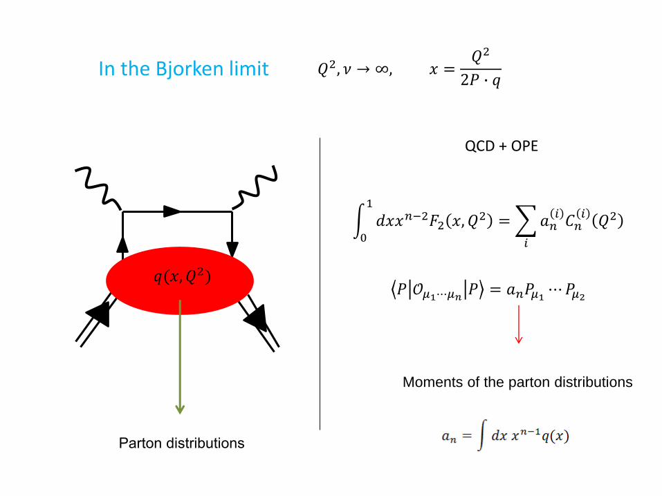
In the Bjorken limit

Parton distributions

𝑄2, 𝜈 → ∞, 𝑥 =𝑄2

2𝑃 ∙ 𝑞

𝑞(𝑥, 𝑄2)

QCD + OPE

Moments of the parton distributions

න0

1

𝑑𝑥𝑥𝑛−2𝐹2 𝑥, 𝑄2 =

𝑖

𝑎𝑛𝑖

𝐶𝑛𝑖

𝑄2

𝑃 𝒪𝜇1⋯𝜇𝑛𝑃 = 𝑎𝑛𝑃𝜇1

⋯ 𝑃𝜇2

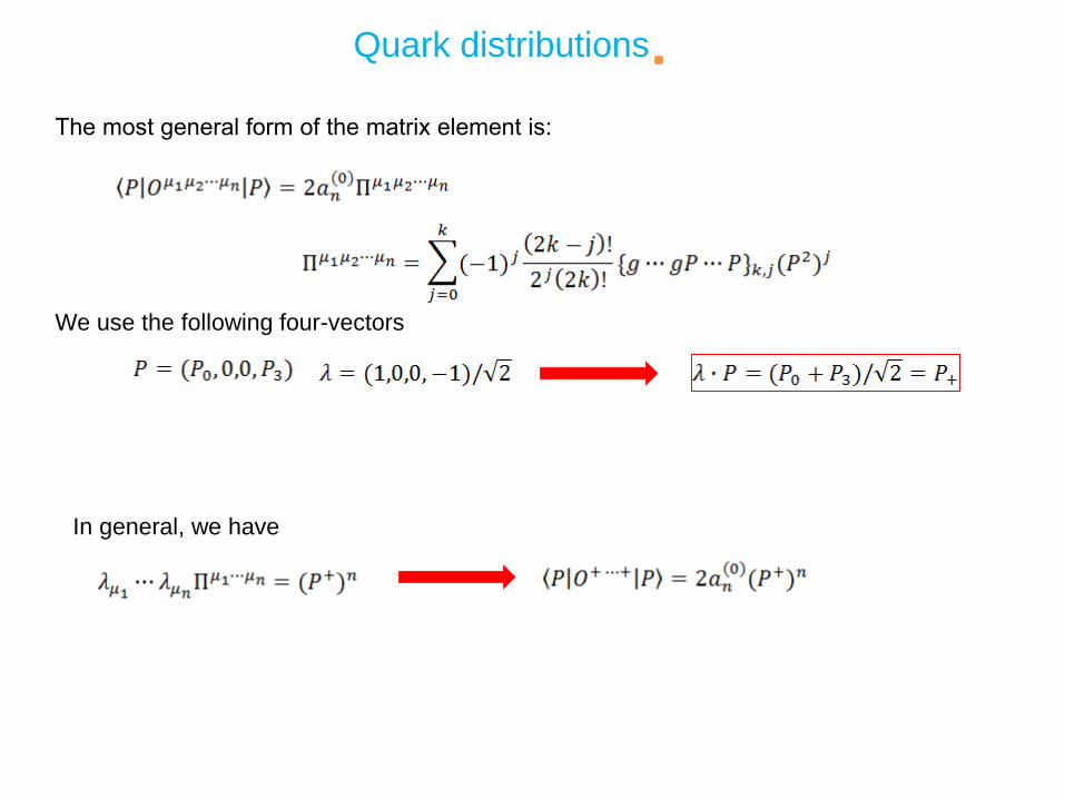
Quark distributions

The most general form of the matrix element is:

We use the following four-vectors

In general, we have

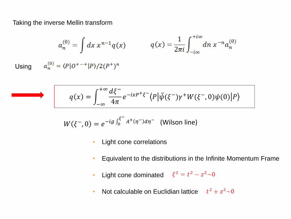
Taking the inverse Mellin transform

𝑞 𝑥 = න−∞

+∞ 𝑑𝜉−

4𝜋𝑒−𝑖𝑥𝑃+𝜉−

𝑃 ത𝜓(𝜉−)𝛾+𝑊(𝜉−, 0)𝜓(0) 𝑃

𝑊 𝜉−, 0 = 𝑒−𝑖𝑔 0𝜉−

𝐴+ 𝜂− 𝑑𝜂−

• Light cone correlations

• Equivalent to the distributions in the Infinite Momentum Frame

• Light cone dominated

• Not calculable on Euclidian lattice

(Wilson line)

Using

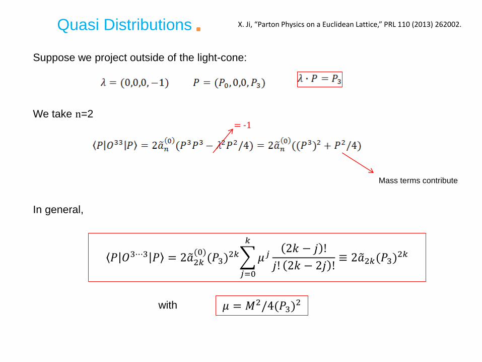
Quasi Distributions

with 𝜇 = 𝑀2/4(𝑃3)2

𝑃 𝑂3⋯3 𝑃 = 2 𝑎2𝑘(0)

(𝑃3)2𝑘

𝑗=0

𝑘

𝜇𝑗2𝑘 − 𝑗 !

𝑗! 2𝑘 − 2𝑗 !≡ 2 𝑎2𝑘(𝑃3)2𝑘

X. Ji, “Parton Physics on a Euclidean Lattice,” PRL 110 (2013) 262002.

Suppose we project outside of the light-cone:

We take n=2 = -1

Mass terms contribute

In general,

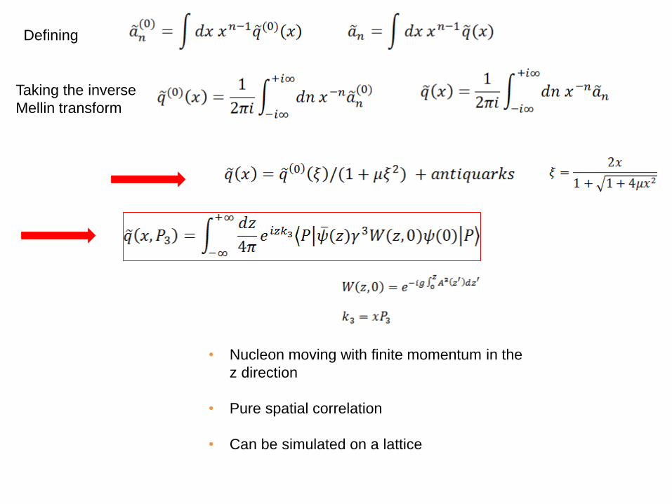
Defining

Taking the inverse

Mellin transform

• Nucleon moving with finite momentum in the

z direction

• Pure spatial correlation

• Can be simulated on a lattice

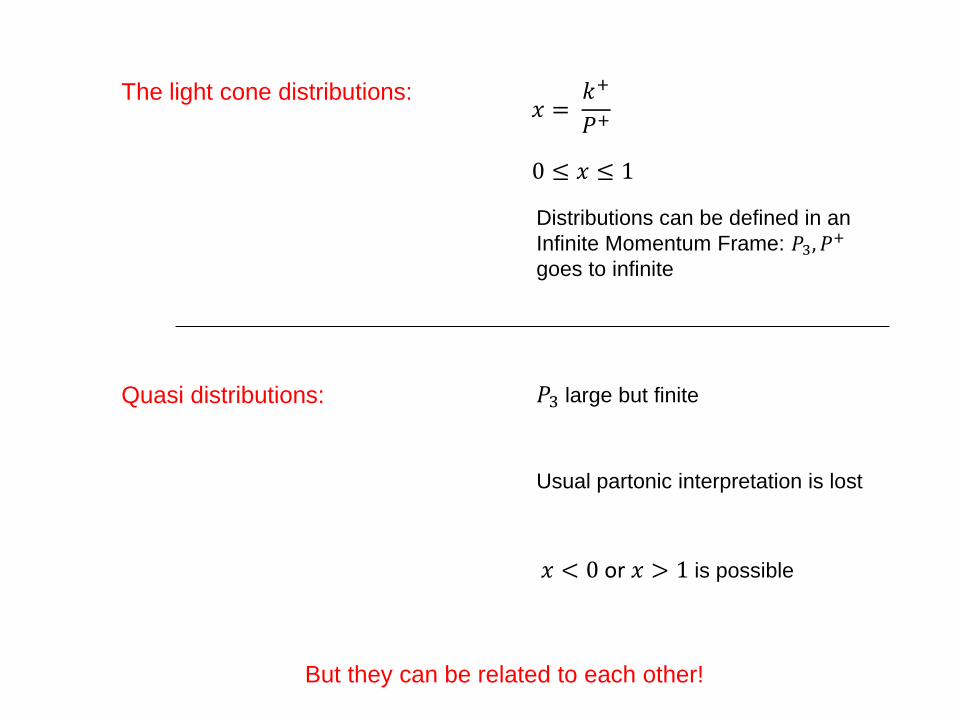
The light cone distributions:𝑥 =

𝑘+

𝑃+

0 ≤ 𝑥 ≤ 1

Quasi distributions:

𝑥 < 0 or 𝑥 > 1 is possible

Usual partonic interpretation is lost

But they can be related to each other!

𝑃3 large but finite

Distributions can be defined in an

Infinite Momentum Frame: 𝑃3, 𝑃+

goes to infinite

Infinite momentum:

Finite momentum:

Largest value at which the calculations are meaningful

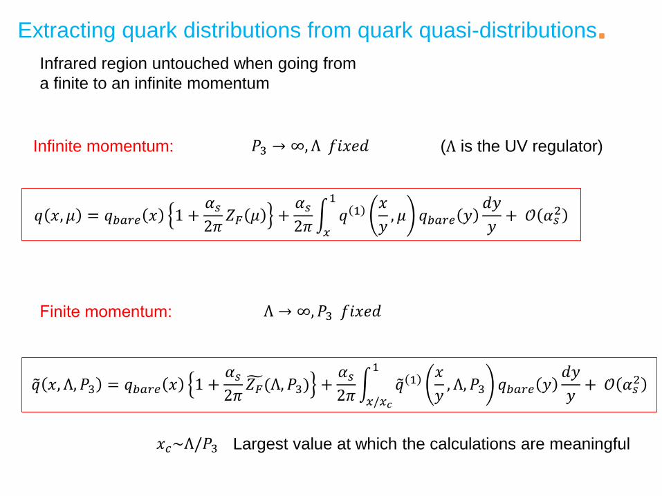
Infrared region untouched when going from

a finite to an infinite momentum

Extracting quark distributions from quark quasi-distributions

𝑃3 → ∞, Λ 𝑓𝑖𝑥𝑒𝑑

Λ → ∞, 𝑃3 𝑓𝑖𝑥𝑒𝑑

𝑥𝑐~Λ/𝑃3

𝑞 𝑥, 𝜇 = 𝑞𝑏𝑎𝑟𝑒 𝑥 1 +𝛼𝑠

2𝜋𝑍𝐹 𝜇 +

𝛼𝑠

2𝜋න

𝑥

1

𝑞 1𝑥

𝑦, 𝜇 𝑞𝑏𝑎𝑟𝑒 𝑦

𝑑𝑦

𝑦+ 𝒪 𝛼𝑠

2

𝑞 𝑥, Λ, 𝑃3 = 𝑞𝑏𝑎𝑟𝑒 𝑥 1 +𝛼𝑠

2𝜋෪𝑍𝐹(Λ, 𝑃3) +

𝛼𝑠

2𝜋න

𝑥/𝑥𝑐

1

𝑞 1𝑥

𝑦, Λ, 𝑃3 𝑞𝑏𝑎𝑟𝑒 𝑦

𝑑𝑦

𝑦+ 𝒪 𝛼𝑠

2

(Λ is the UV regulator)

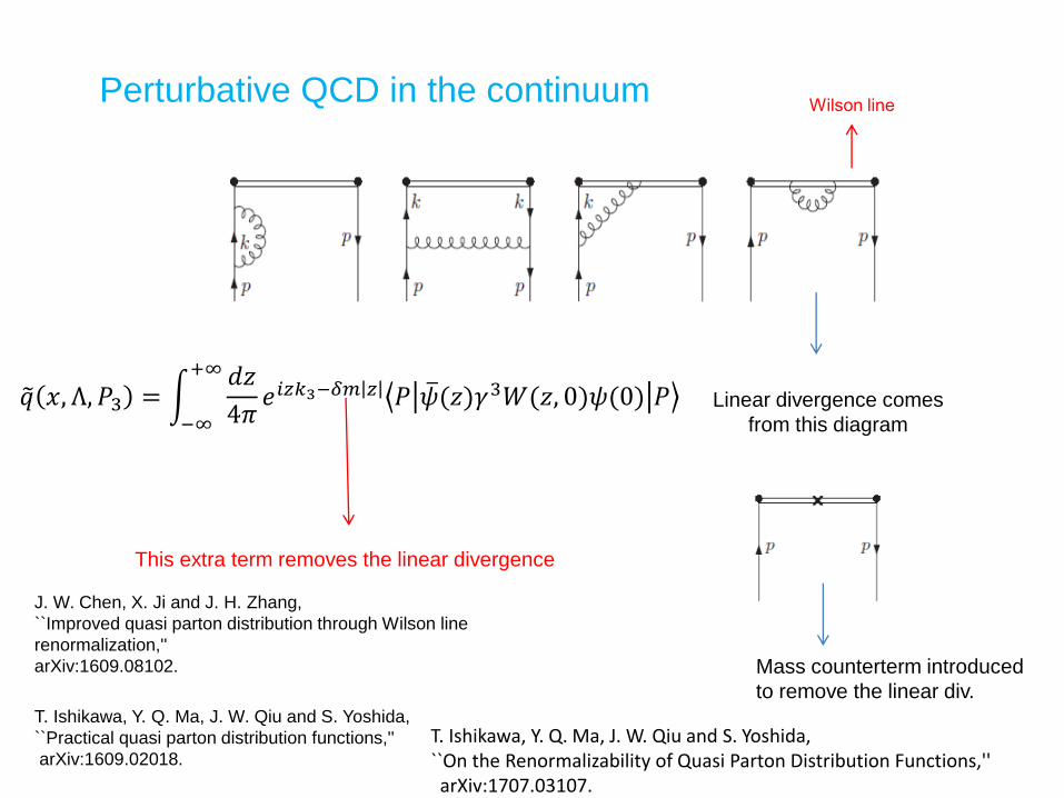
Perturbative QCD in the continuum

Linear divergence comes

from this diagram

Mass counterterm introduced

to remove the linear div.T. Ishikawa, Y. Q. Ma, J. W. Qiu and S. Yoshida,

``Practical quasi parton distribution functions,''

arXiv:1609.02018.

J. W. Chen, X. Ji and J. H. Zhang,

``Improved quasi parton distribution through Wilson line

renormalization,''

arXiv:1609.08102.

This extra term removes the linear divergence

Wilson line

𝑞 𝑥, Λ, 𝑃3 = න−∞

+∞ 𝑑𝑧

4𝜋𝑒𝑖𝑧𝑘3−𝛿𝑚 𝑧 𝑃 ത𝜓(𝑧)𝛾3𝑊(𝑧, 0)𝜓(0) 𝑃

T. Ishikawa, Y. Q. Ma, J. W. Qiu and S. Yoshida, ``On the Renormalizability of Quasi Parton Distribution Functions,''arXiv:1707.03107.

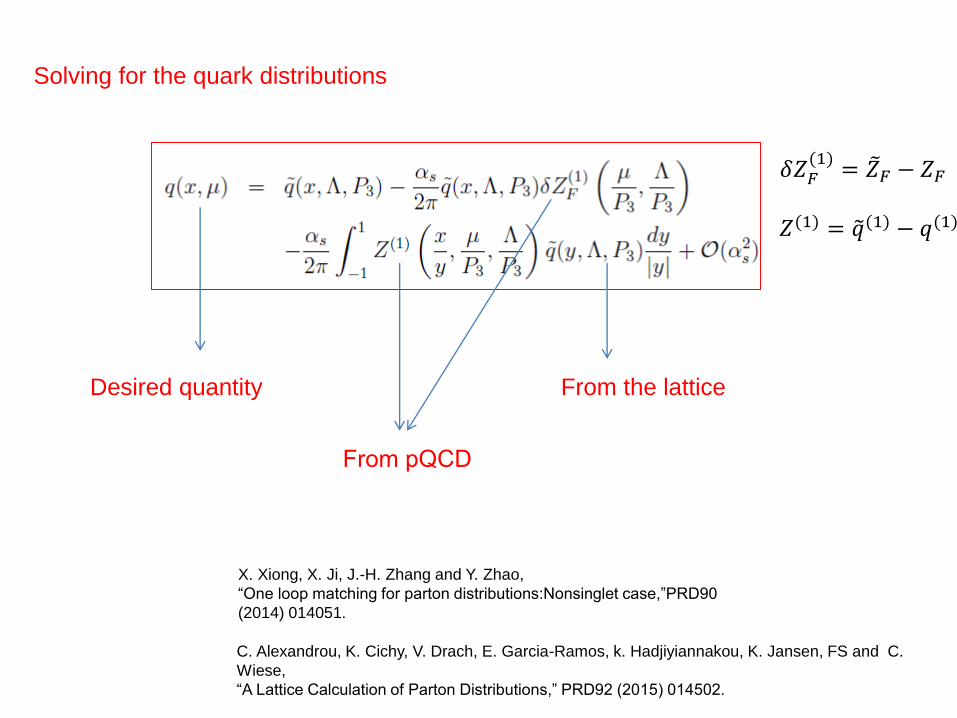
Solving for the quark distributions

𝛿𝑍𝐹(1)

= ෨𝑍𝐹 − 𝑍𝐹

𝑍(1) = 𝑞(1) − 𝑞(1)

Desired quantity From the lattice

From pQCD

C. Alexandrou, K. Cichy, V. Drach, E. Garcia-Ramos, k. Hadjiyiannakou, K. Jansen, FS and C.

Wiese,

“A Lattice Calculation of Parton Distributions,” PRD92 (2015) 014502.

X. Xiong, X. Ji, J.-H. Zhang and Y. Zhao,

“One loop matching for parton distributions:Nonsinglet case,”PRD90

(2014) 014051.

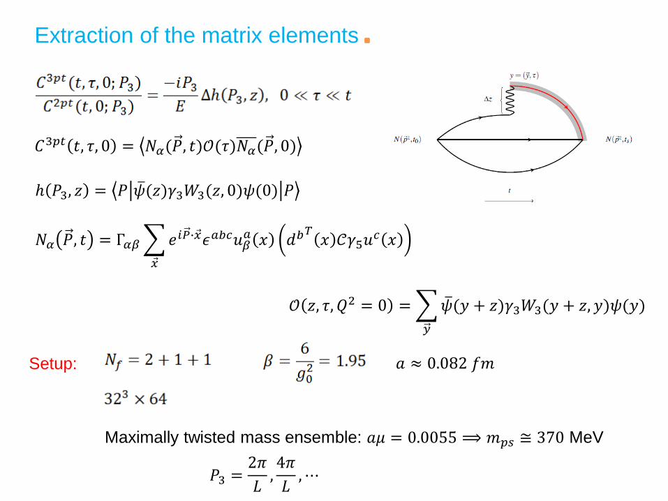
Extraction of the matrix elements

Maximally twisted mass ensemble: 𝑎𝜇 = 0.0055 ⟹ 𝑚𝑝𝑠 ≅ 370 MeV

𝑃3 =2𝜋

𝐿,4𝜋

𝐿, ⋯

𝑎 ≈ 0.082 𝑓𝑚

ℎ 𝑃3, 𝑧 = 𝑃 ത𝜓(𝑧)𝛾3𝑊3(𝑧, 0)𝜓(0) 𝑃

𝐶3𝑝𝑡 𝑡, 𝜏, 0 = 𝑁𝛼(𝑃, 𝑡)𝒪(𝜏)𝑁𝛼(𝑃, 0)

𝑁𝛼 𝑃, 𝑡 = Γ𝛼𝛽

Ԧ𝑥

𝑒𝑖𝑃∙ Ԧ𝑥𝜖𝑎𝑏𝑐𝑢𝛽𝑎 𝑥 𝑑𝑏𝑇

𝑥 𝒞𝛾5𝑢𝑐 𝑥

𝒪 𝑧, 𝜏, 𝑄2 = 0 =

𝑦

ത𝜓(𝑦 + 𝑧)𝛾3𝑊3(𝑦 + 𝑧, 𝑦)𝜓(𝑦)

Setup:

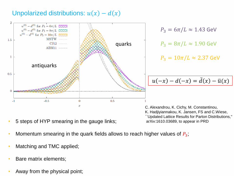
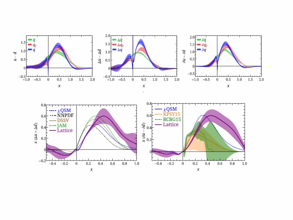
Unpolarized distributions: 𝑢 𝑥 − 𝑑 𝑥

• 5 steps of HYP smearing in the gauge links;

• Momentum smearing in the quark fields allows to reach higher values of 𝑃3;

• Matching and TMC applied;

• Bare matrix elements;

• Away from the physical point;

𝑃3 = 6𝜋/𝐿 ≈ 1.43 GeV

𝑃3 = 8𝜋/𝐿 ≈ 1.90 GeV

𝑃3 = 10𝜋/𝐿 ≈ 2.37 GeV

antiquarks

quarks

𝑢 −𝑥 − 𝑑 −𝑥 = ҧ𝑑 𝑥 − ത𝑢(𝑥)

C. Alexandrou, K. Cichy, M. Constantinou,

K. Hadjiyiannakou, K. Jansen, FS and C.Wiese,

``Updated Lattice Results for Parton Distributions,''

arXiv:1610.03689, to appear in PRD

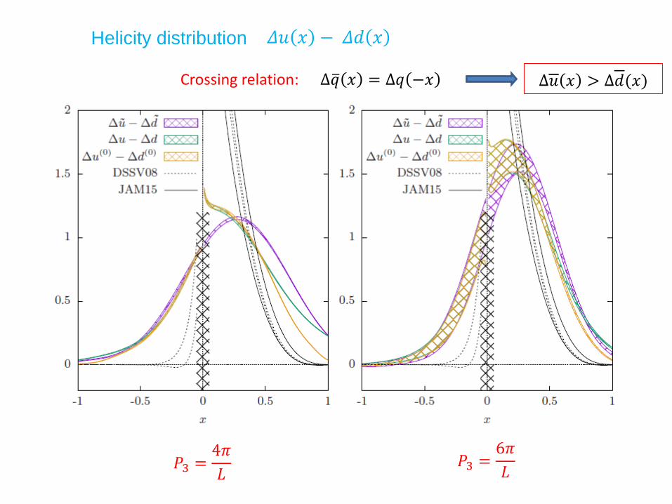
Crossing relation:

𝛥𝑢 𝑥 − 𝛥𝑑 𝑥

Δ𝑢 𝑥 > Δ𝑑(𝑥)

𝑃3 =4𝜋

𝐿𝑃3 =

6𝜋

𝐿

Δത𝑞 𝑥 = Δ𝑞 −𝑥

Helicity distribution

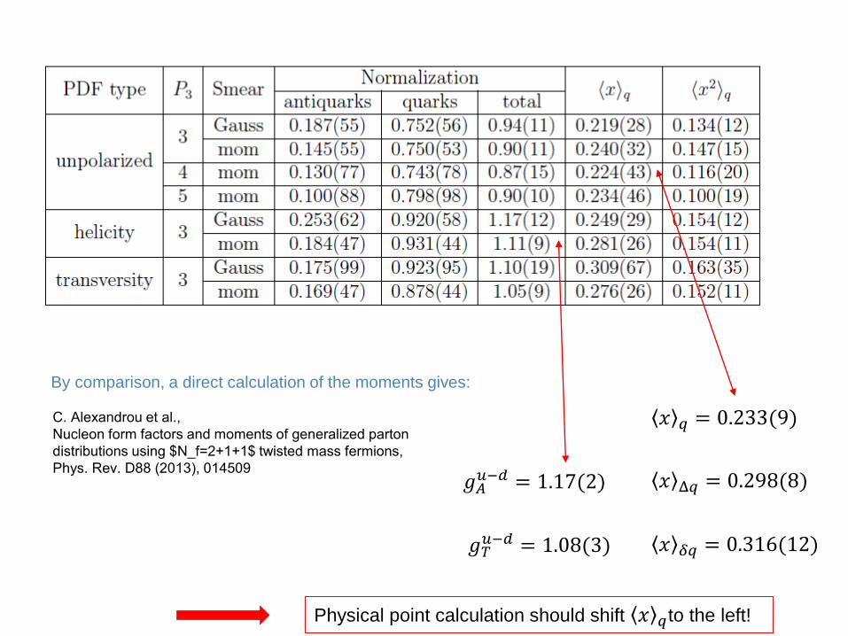
By comparison, a direct calculation of the moments gives:

𝑔𝐴𝑢−𝑑 = 1.17(2)

𝑔𝑇𝑢−𝑑 = 1.08(3)

𝑥 𝑞 = 0.233(9)

𝑥 Δ𝑞 = 0.298(8)

𝑥 𝛿𝑞 = 0.316(12)

C. Alexandrou et al.,

Nucleon form factors and moments of generalized parton

distributions using $N_f=2+1+1$ twisted mass fermions,

Phys. Rev. D88 (2013), 014509

Physical point calculation should shift 𝑥 𝑞to the left!

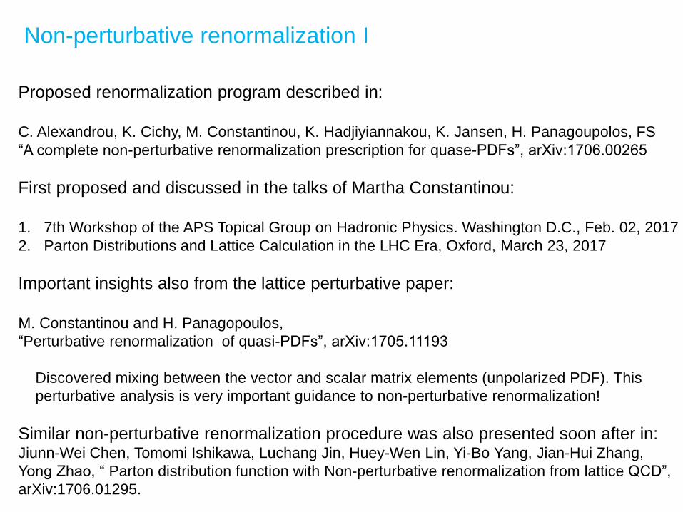
Non-perturbative renormalization I

Proposed renormalization program described in:

C. Alexandrou, K. Cichy, M. Constantinou, K. Hadjiyiannakou, K. Jansen, H. Panagoupolos, FS

“A complete non-perturbative renormalization prescription for quase-PDFs”, arXiv:1706.00265

First proposed and discussed in the talks of Martha Constantinou:

1. 7th Workshop of the APS Topical Group on Hadronic Physics. Washington D.C., Feb. 02, 2017

2. Parton Distributions and Lattice Calculation in the LHC Era, Oxford, March 23, 2017

Important insights also from the lattice perturbative paper:

M. Constantinou and H. Panagopoulos,

“Perturbative renormalization of quasi-PDFs”, arXiv:1705.11193

Discovered mixing between the vector and scalar matrix elements (unpolarized PDF). This

perturbative analysis is very important guidance to non-perturbative renormalization!

Similar non-perturbative renormalization procedure was also presented soon after in:Jiunn-Wei Chen, Tomomi Ishikawa, Luchang Jin, Huey-Wen Lin, Yi-Bo Yang, Jian-Hui Zhang,

Yong Zhao, “ Parton distribution function with Non-perturbative renormalization from lattice QCD”,

arXiv:1706.01295.

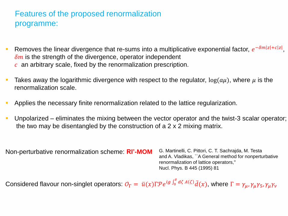
Features of the proposed renormalization

programme:

▪ Removes the linear divergence that re-sums into a multiplicative exponential factor, 𝑒−𝛿𝑚 𝑧 +𝑐 𝑧 ,

𝛿𝑚 is the strength of the divergence, operator independent

𝑐 an arbitrary scale, fixed by the renormalization prescription.

▪ Takes away the logarithmic divergence with respect to the regulator, log(𝑎𝜇), where 𝜇 is the

renormalization scale.

▪ Applies the necessary finite renormalization related to the lattice regularization.

▪ Unpolarized – eliminates the mixing between the vector operator and the twist-3 scalar operator;

the two may be disentangled by the construction of a 2 x 2 mixing matrix.

Non-perturbative renormalization scheme: RI’-MOM

Considered flavour non-singlet operators: 𝒪Γ = ത𝑢(𝑥)Γ𝒫𝑒𝑖𝑔 0𝑧

𝑑𝜁 𝐴 𝜁 ҧ𝑑(𝑥), where Γ = 𝛾𝜇 , 𝛾𝜇𝛾5, 𝛾𝜇𝛾𝜈

G. Martinelli, C. Pittori, C. T. Sachrajda, M. Testa

and A. Vladikas, ``A General method for nonperturbative

renormalization of lattice operators,''

Nucl. Phys. B 445 (1995) 81

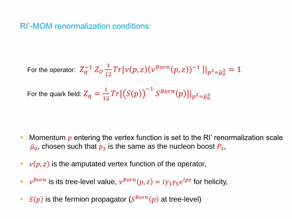
RI’-MOM renormalization conditions:

For the operator: 𝑍𝑞−1 𝑍𝒪

1

12𝑇𝑟[𝜈 𝑝, 𝑧 𝜈𝐵𝑜𝑟𝑛 𝑝, 𝑧 )−1 |𝑝2=ഥ𝜇0

2 = 1

For the quark field: 𝑍𝑞 =1

12𝑇𝑟[ 𝑆 𝑝

−1𝑆𝐵𝑜𝑟𝑛 𝑝 ]|𝑝2=ഥ𝜇0

2

▪ Momentum 𝑝 entering the vertex function is set to the RI’ renormalization scale

ҧ𝜇0, chosen such that 𝑝3 is the same as the nucleon boost 𝑃3,

▪ 𝜈 𝑝, 𝑧 is the amputated vertex function of the operator,

▪ 𝜈𝐵𝑜𝑟𝑛 is its tree-level value, 𝜈𝐵𝑜𝑟𝑛 𝑝, 𝑧 = 𝑖𝛾3𝛾5𝑒𝑖𝑝𝑧 for helicity,

▪ 𝑆 𝑝 is the fermion propagator (𝑆𝐵𝑜𝑟𝑛 𝑝 at tree-level)

▪ The vertex functions 𝜈(𝑝) contain the same linear divergence as the nucleon

matrix elements.

▪ This is crucial, as it allows the extraction of the exponential together with the

multiplicative Z-factor.

▪ 𝑍𝒪 can be factorized as 𝑍𝒪 = ҧ𝑍𝒪 𝑒+𝛿𝑚𝑧

𝑎−𝑐 𝑧

, where ҧ𝑍𝒪 is the multiplicative Z-factor

of the operator.

▪ Note that the exponential comes with a different sign compared to the nucleon

matrix element (𝑍𝒪 is related to the inverse of the vertex function).

▪ Consequently, the above renormalization condition handles all the divergences

which are present in the matrix element under consideration.

▪ In the absence of a Wilson line (𝑧 = 0), the renormalization functions reduce to

the local currents, free of any power divergence, e.g. for helicity 𝑍𝒪 𝑧 = 0 ≡ 𝑍𝐴.

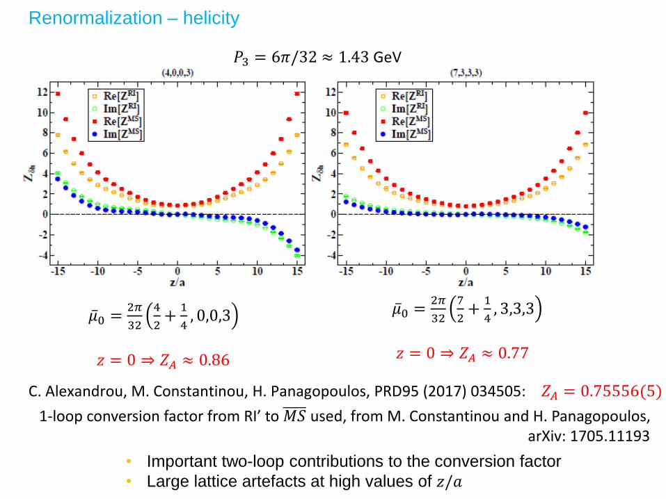
Renormalization – helicity

𝑃3 = 6𝜋/32 ≈ 1.43 GeV

ҧ𝜇0 =2𝜋

32

4

2+

1

4, 0,0,3

𝑧 = 0 ⇒ 𝑍𝐴 ≈ 0.86

ҧ𝜇0 =2𝜋

32

7

2+

1

4, 3,3,3

𝑧 = 0 ⇒ 𝑍𝐴 ≈ 0.77

C. Alexandrou, M. Constantinou, H. Panagopoulos, PRD95 (2017) 034505: 𝑍𝐴 = 0.75556(5)

• Important two-loop contributions to the conversion factor

• Large lattice artefacts at high values of 𝑧/𝑎

1-loop conversion factor from RI’ to 𝑀𝑆 used, from M. Constantinou and H. Panagopoulos,arXiv: 1705.11193

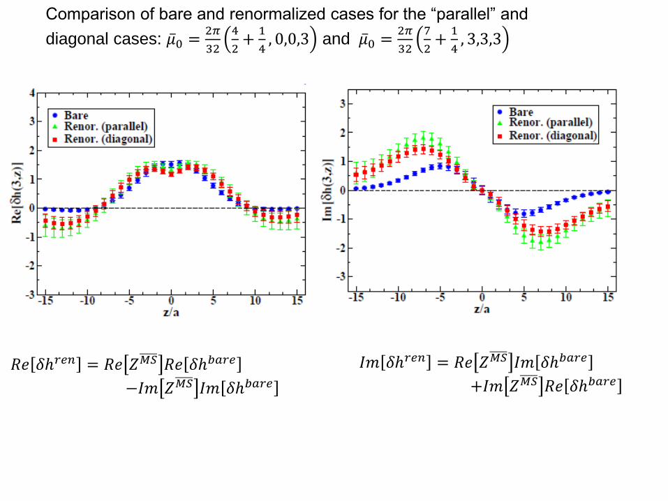
Comparison of bare and renormalized cases for the “parallel” and

diagonal cases: ҧ𝜇0 =2𝜋

32

4

2+

1

4, 0,0,3 and ҧ𝜇0 =

2𝜋

32

7

2+

1

4, 3,3,3

𝑅𝑒 𝛿ℎ𝑟𝑒𝑛 = 𝑅𝑒 𝑍𝑀𝑆 𝑅𝑒 𝛿ℎ𝑏𝑎𝑟𝑒

−𝐼𝑚 𝑍𝑀𝑆 𝐼𝑚 𝛿ℎ𝑏𝑎𝑟𝑒

𝐼𝑚 𝛿ℎ𝑟𝑒𝑛 = 𝑅𝑒 𝑍𝑀𝑆 𝐼𝑚 𝛿ℎ𝑏𝑎𝑟𝑒

+𝐼𝑚 𝑍𝑀𝑆 𝑅𝑒 𝛿ℎ𝑏𝑎𝑟𝑒

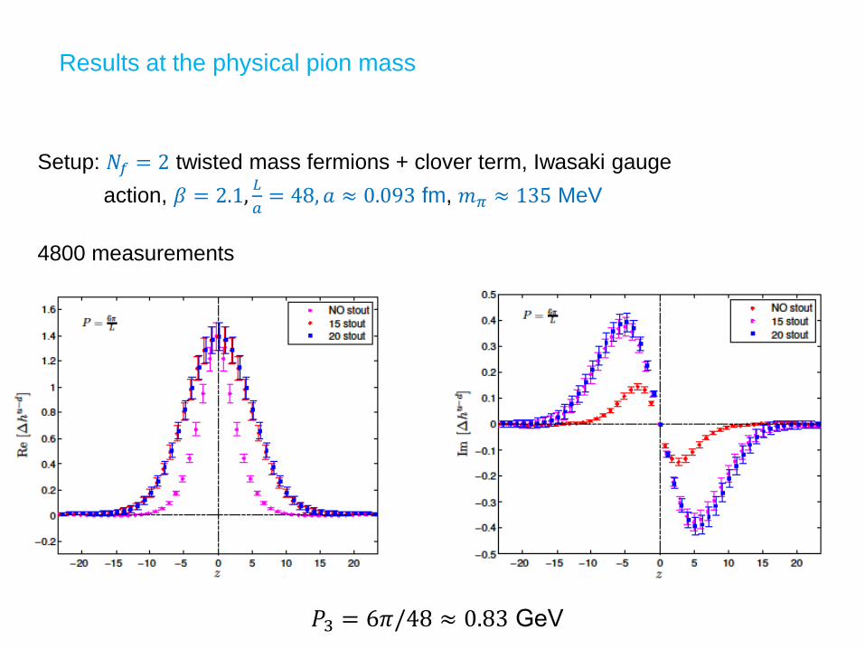
Results at the physical pion mass

Setup: 𝑁𝑓 = 2 twisted mass fermions + clover term, Iwasaki gauge

action, 𝛽 = 2.1,𝐿

𝑎= 48, 𝑎 ≈ 0.093 fm, 𝑚𝜋 ≈ 135 MeV

4800 measurements

𝑃3 = 6𝜋/48 ≈ 0.83 GeV

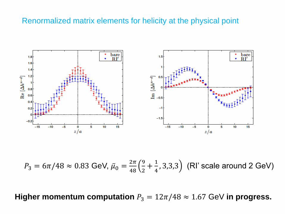
Renormalized matrix elements for helicity at the physical point

𝑃3 = 6𝜋/48 ≈ 0.83 GeV, ҧ𝜇0 =2𝜋

48

9

2+

1

4, 3,3,3 (RI’ scale around 2 GeV)

Higher momentum computation 𝑃3 = 12𝜋/48 ≈ 1.67 GeV in progress.

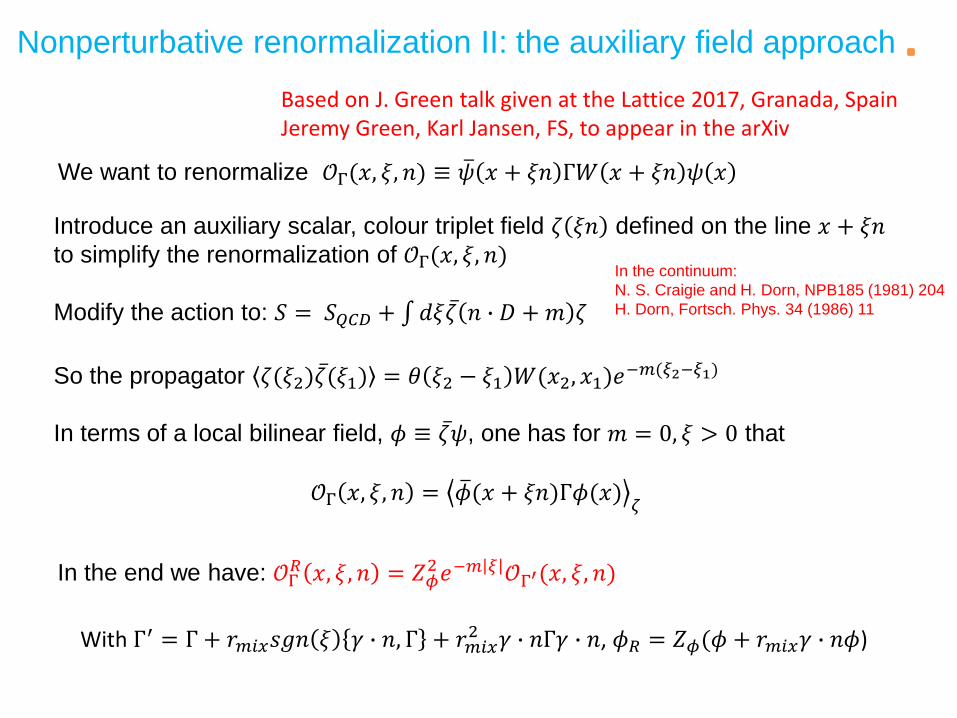
Nonperturbative renormalization II: the auxiliary field approach

We want to renormalize 𝒪Γ(𝑥, 𝜉, 𝑛) ≡ ത𝜓 𝑥 + 𝜉𝑛 Γ𝑊 𝑥 + 𝜉𝑛 𝜓 𝑥

Introduce an auxiliary scalar, colour triplet field 𝜁 𝜉𝑛 defined on the line 𝑥 + 𝜉𝑛to simplify the renormalization of 𝒪Γ(𝑥, 𝜉, 𝑛)

Modify the action to: 𝑆 = 𝑆𝑄𝐶𝐷 + 𝑑𝜉 ҧ𝜁 𝑛 ∙ 𝐷 + 𝑚 𝜁

So the propagator 𝜁(𝜉2) ҧ𝜁(𝜉1) = 𝜃 𝜉2 − 𝜉1 𝑊(𝑥2, 𝑥1)𝑒−𝑚(𝜉2−𝜉1)

In terms of a local bilinear field, 𝜙 ≡ ҧ𝜁𝜓, one has for 𝑚 = 0, 𝜉 > 0 that

𝒪Γ 𝑥, 𝜉, 𝑛 = ത𝜙(𝑥 + 𝜉𝑛)Γ𝜙(𝑥)𝜁

In the end we have: 𝒪Γ𝑅 𝑥, 𝜉, 𝑛 = 𝑍𝜙

2 𝑒−𝑚 𝜉 𝒪Γ′(𝑥, 𝜉, 𝑛)

With Γ′ = Γ + 𝑟𝑚𝑖𝑥𝑠𝑔𝑛 𝜉 𝛾 ∙ 𝑛, Γ + 𝑟𝑚𝑖𝑥2 𝛾 ∙ 𝑛Γ𝛾 ∙ 𝑛, 𝜙𝑅 = 𝑍𝜙(𝜙 + 𝑟𝑚𝑖𝑥𝛾 ∙ 𝑛𝜙)

Based on J. Green talk given at the Lattice 2017, Granada, SpainJeremy Green, Karl Jansen, FS, to appear in the arXiv

In the continuum:

N. S. Craigie and H. Dorn, NPB185 (1981) 204

H. Dorn, Fortsch. Phys. 34 (1986) 11

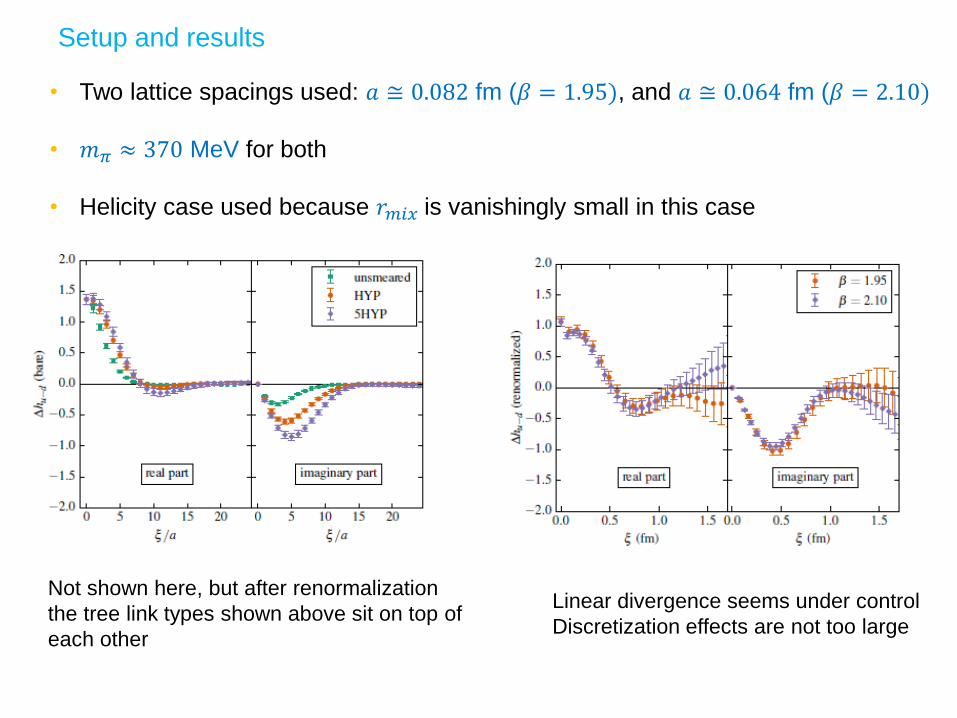
• Two lattice spacings used: 𝑎 ≅ 0.082 fm (𝛽 = 1.95), and 𝑎 ≅ 0.064 fm (𝛽 = 2.10)

• 𝑚𝜋 ≈ 370 MeV for both

• Helicity case used because 𝑟𝑚𝑖𝑥 is vanishingly small in this case

Setup and results

Linear divergence seems under control

Discretization effects are not too large

Not shown here, but after renormalization

the tree link types shown above sit on top of

each other

Summary

Calculation of bare non▪ -singlet quark distributions in lattice QCD at large values

of the nucleon momentum;

Asymmetry in the light antiquark distributions for all cases appears naturally; ▪

Calculated moments agree with previous calculation using a different method;▪

A full renormalization prescription to handle all the divergences present in the▪

matrix elements for the quasi-PDFs was presented;

Standard logarithmic divergence handled with ҧ𝑍𝒪

Power divergence renormalized with 𝑒+𝛿𝑚𝑧

𝑎−𝑐 𝑧

For unpolarized, mixing between vector and scalar matrix elements ▪ – needs

computation of a mixing matrix;

For conversion to ▪ 𝑀𝑆, one needs to take care of truncation effects in the

conversion factor. 𝐼𝑚 𝑍𝑀𝑆 should vanish for all 𝑧;

• We have presented preliminary bare and renormalized results at the

physical points – statistics constantly increasing, in particular at a

higher momentum;

• Alternative nonperturbative renormalization was presented. The

renormalization of the non-local operator is replaces by the

renormalization of a local quark bilinear;

• Increasingly rapid progress in this field.

Thanks for the attention!

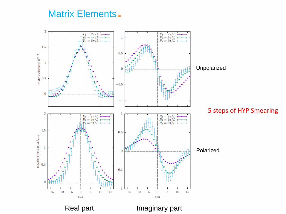
Matrix Elements

5 steps of HYP Smearing

Real part Imaginary part

Unpolarized

Polarized

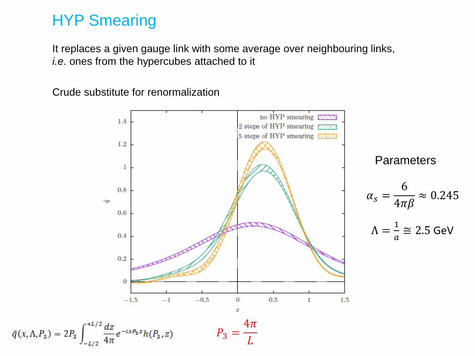
HYP Smearing

It replaces a given gauge link with some average over neighbouring links,

i.e. ones from the hypercubes attached to it

Crude substitute for renormalization

Parameters

𝑃3 =4𝜋

𝐿

𝛼𝑠 =6

4𝜋𝛽≈ 0.245

Λ =1

𝑎≅ 2.5 GeV

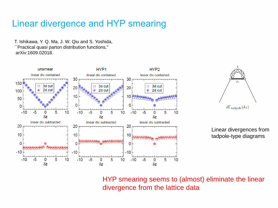
Linear divergence and HYP smearing

Linear divergences from

tadpole-type diagrams

HYP smearing seems to (almost) eliminate the linear

divergence from the lattice data

T. Ishikawa, Y. Q. Ma, J. W. Qiu and S. Yoshida,

``Practical quasi parton distribution functions,''

arXiv:1609.02018.

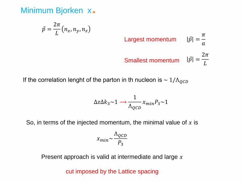
Minimum Bjorken x

Largest momentum

Smallest momentum

Present approach is valid at intermediate and large 𝑥

cut imposed by the Lattice spacing

If the correlation lenght of the parton in th nucleon is ~ 1/Λ𝑄𝐶𝐷

Δ𝑧Δ𝑘3~1 ⟶1

Λ𝑄𝐶𝐷𝑥𝑚𝑖𝑛𝑃3~1

𝑥𝑚𝑖𝑛~Λ𝑄𝐶𝐷

𝑃3

So, in terms of the injected momentum, the minimal value of 𝑥 is

Ԧ𝑝 =2𝜋

𝐿𝑛𝑥 , 𝑛𝑦 , 𝑛𝑧

Ԧ𝑝 =𝜋

𝑎

Ԧ𝑝 =2𝜋

𝐿

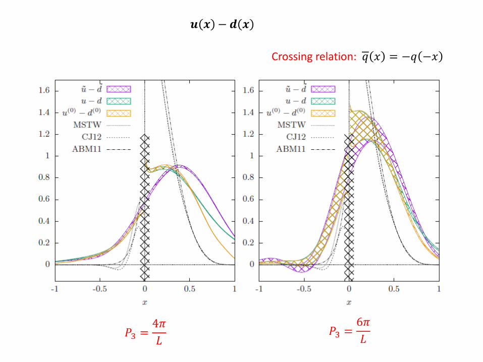
𝑞 𝑥 = −𝑞 −𝑥Crossing relation:

𝑃3 =4𝜋

𝐿𝑃3 =

6𝜋

𝐿

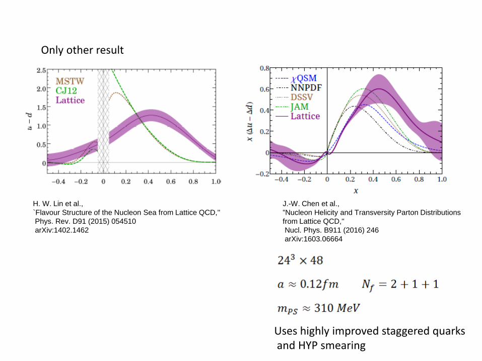
Only other result

H. W. Lin et al.,

`Flavour Structure of the Nucleon Sea from Lattice QCD,''

Phys. Rev. D91 (2015) 054510

arXiv:1402.1462

Uses highly improved staggered quarksand HYP smearing

J.-W. Chen et al.,

“Nucleon Helicity and Transversity Parton Distributions

from Lattice QCD,''

Nucl. Phys. B911 (2016) 246

arXiv:1603.06664

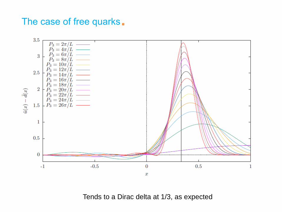
The case of free quarks

Tends to a Dirac delta at 1/3, as expected

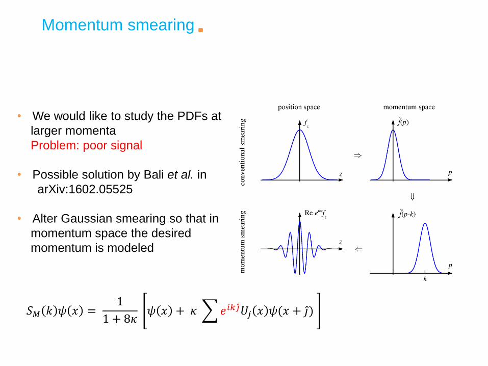
Momentum smearing

• We would like to study the PDFs at

larger momenta

Problem: poor signal

• Possible solution by Bali et al. in

arXiv:1602.05525

• Alter Gaussian smearing so that in

momentum space the desired

momentum is modeled

𝑆𝑀 𝑘 𝜓 𝑥 =1

1 + 8𝜅𝜓 𝑥 + 𝜅 𝑒𝑖𝑘 Ƹ𝑗𝑈𝑗 𝑥 𝜓(𝑥 + Ƹ𝑗)

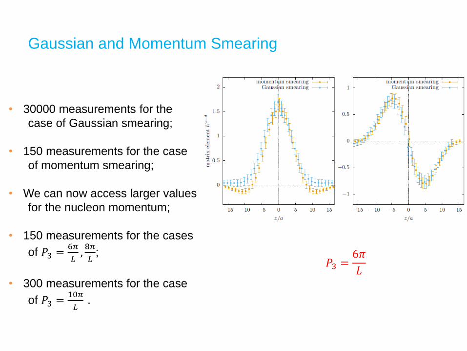
Gaussian and Momentum Smearing

𝑃3 =6𝜋

𝐿

• 30000 measurements for the

case of Gaussian smearing;

• 150 measurements for the case

of momentum smearing;

• We can now access larger values

for the nucleon momentum;

• 150 measurements for the cases

of 𝑃3 =6𝜋

𝐿,

8𝜋

𝐿;

• 300 measurements for the case

of 𝑃3 =10𝜋

𝐿.

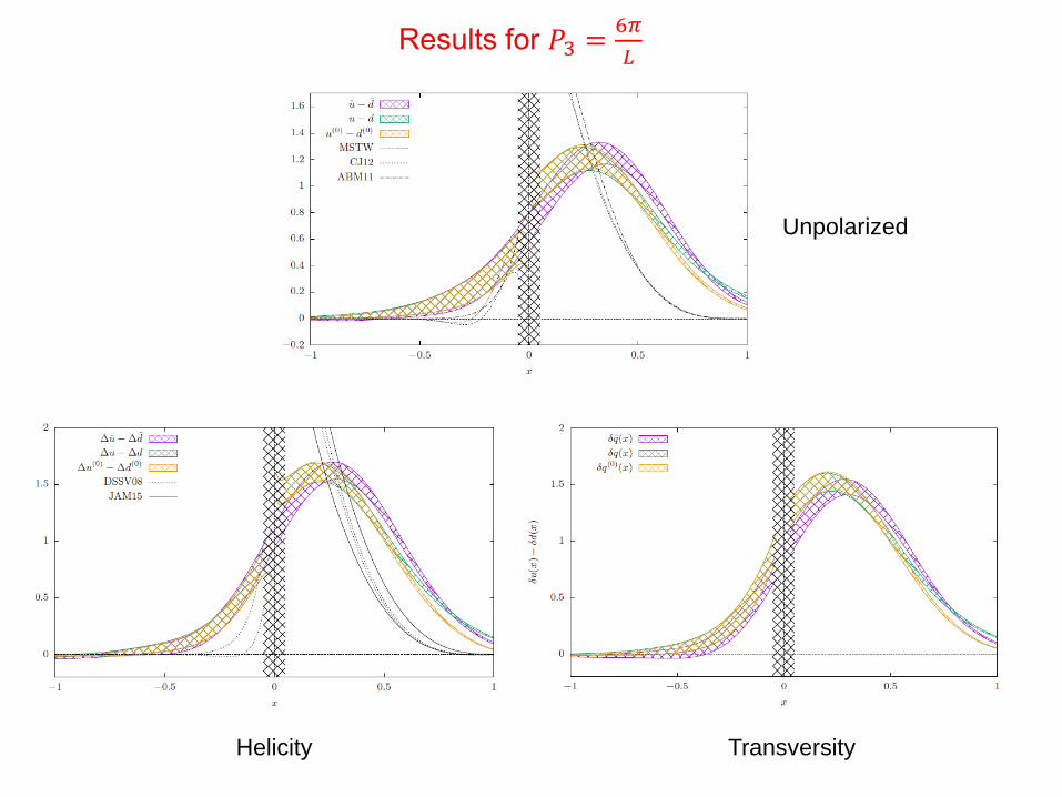
Results for 𝑃3 =6𝜋

𝐿

Unpolarized

Helicity Transversity

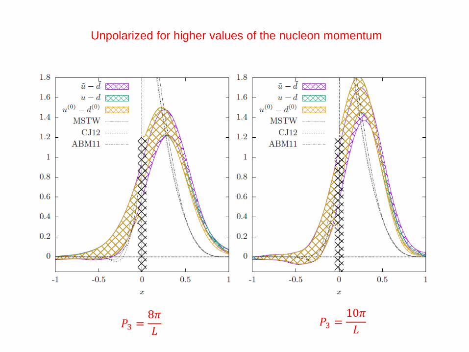
Unpolarized for higher values of the nucleon momentum

𝑃3 =8𝜋

𝐿𝑃3 =

10𝜋

𝐿

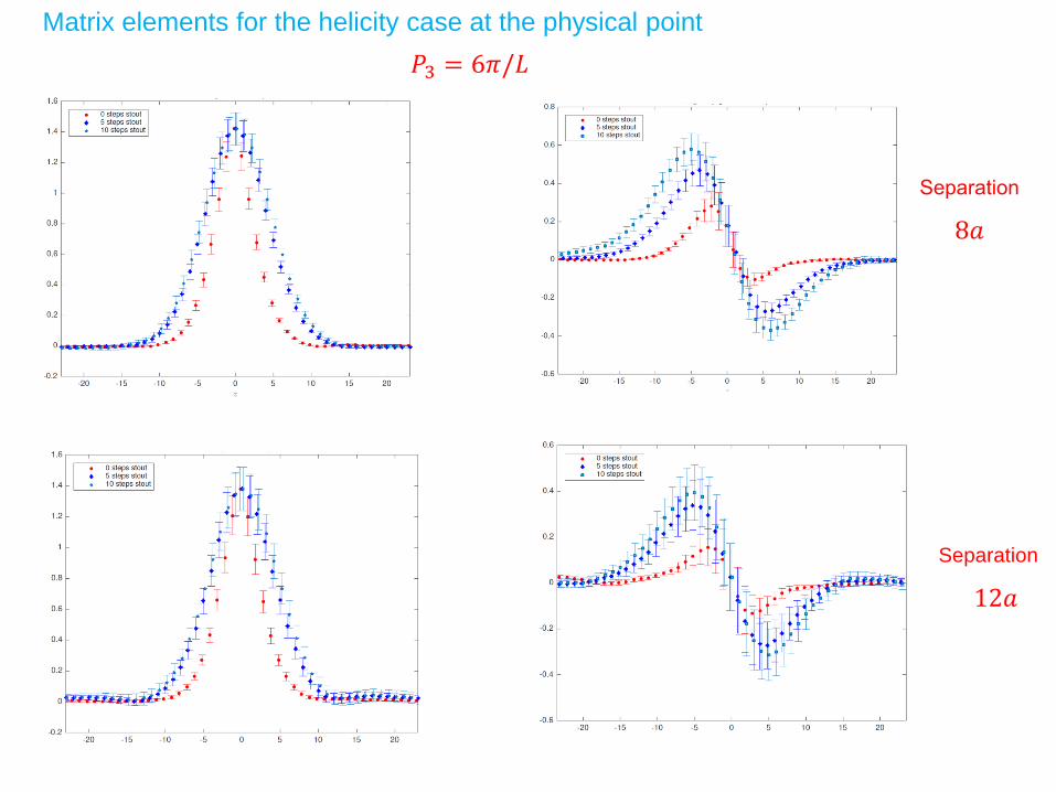
Matrix elements for the helicity case at the physical point

Separation

8𝑎

Separation

12𝑎

𝑃3 = 6𝜋/𝐿

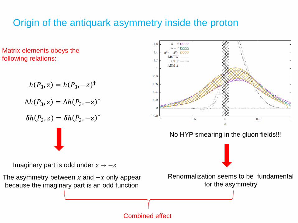
Origin of the antiquark asymmetry inside the proton

No HYP smearing in the gluon fields!!!

ℎ 𝑃3, 𝑧 = ℎ 𝑃3, −𝑧 †

Δℎ 𝑃3, 𝑧 = Δℎ 𝑃3, −𝑧 †

𝛿ℎ 𝑃3, 𝑧 = 𝛿ℎ 𝑃3, −𝑧 †

Matrix elements obeys the

following relations:

Renormalization seems to be fundamental

for the asymmetry

Imaginary part is odd under 𝑧 → −𝑧

The asymmetry between 𝑥 and −𝑥 only appear

because the imaginary part is an odd function

Combined effect

➢ First attempts of a direct QCD calculation of quark distributions;

➢ Valuable information from intermediate to large x region;

➢ Asymmetric sea appears naturally. Imaginary part plays a fundamental role;

➢ Non perturbative renormalization is on its way;

➢ Momentum Smearing: it allows access to higher momentum;

➢ Computation at the physical mass has started – smaller number of configurations available at the moment;

➢ Go to the continuum;

➢ Singlet distributions, gluon distributions, TMDs, etc

➢ Much to be done!

Summary & Outline

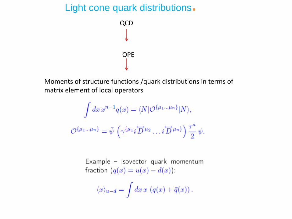
Light cone quark distributions

QCD

OPE

Moments of structure functions /quark distributions in terms ofmatrix element of local operators

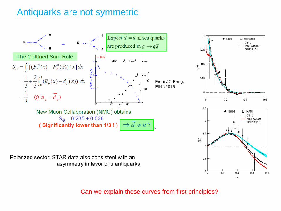
Antiquarks are not symmetric

Can we explain these curves from first principles?

From JC Peng,

EINN2015

Polarized sector: STAR data also consistent with an

asymmetry in favor of u antiquarks

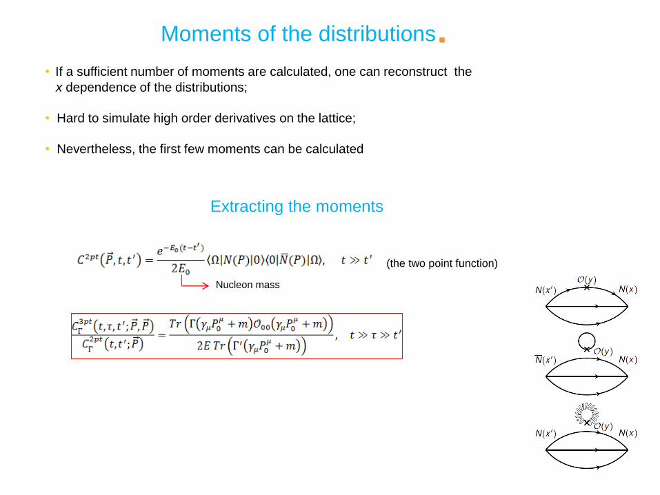
Moments of the distributions

• If a sufficient number of moments are calculated, one can reconstruct the

x dependence of the distributions;

• Hard to simulate high order derivatives on the lattice;

• Nevertheless, the first few moments can be calculated

Extracting the moments

(the two point function)

Nucleon mass

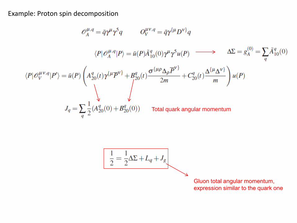
Example: Proton spin decomposition

Total quark angular momentum

Gluon total angular momentum,

expression similar to the quark one

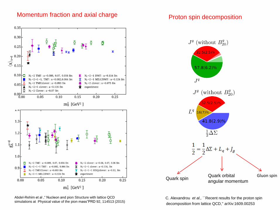
Proton spin decompositionMomentum fraction and axial charge

Quark spinQuark orbital

angular momentum

Gluon spin

Abdel-Rehim et al ,“ Nucleon and pion Structure with lattice QCD

simulations at Physical value of the pion mass”PRD 92, 114513 (2015)C. Alexandrou et al., ``Recent results for the proton spin

decomposition from lattice QCD,'' arXiv:1609.00253

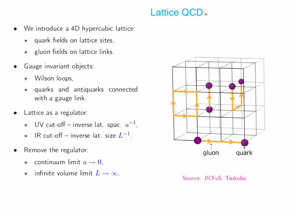
Lattice QCD

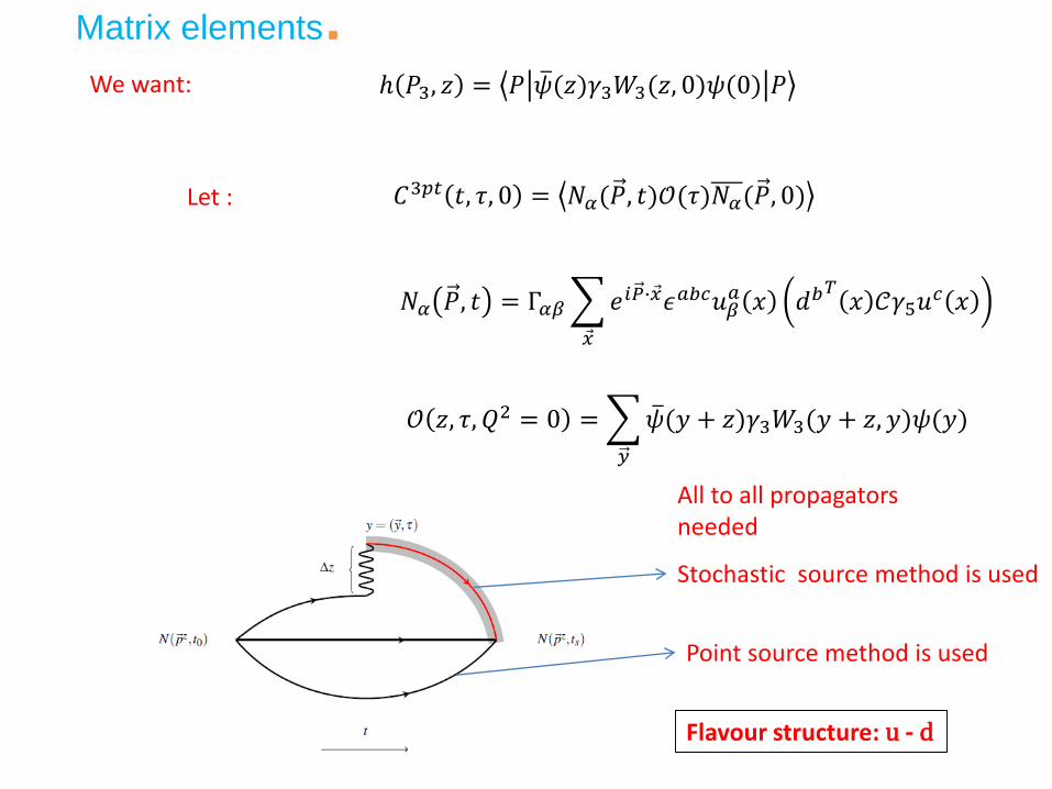
We want:

Let :

All to all propagators needed

Stochastic source method is used

Flavour structure: u - d

Point source method is used

ℎ 𝑃3, 𝑧 = 𝑃 ത𝜓(𝑧)𝛾3𝑊3(𝑧, 0)𝜓(0) 𝑃

𝐶3𝑝𝑡 𝑡, 𝜏, 0 = 𝑁𝛼(𝑃, 𝑡)𝒪(𝜏)𝑁𝛼(𝑃, 0)

𝑁𝛼 𝑃, 𝑡 = Γ𝛼𝛽

Ԧ𝑥

𝑒𝑖𝑃∙ Ԧ𝑥𝜖𝑎𝑏𝑐𝑢𝛽𝑎 𝑥 𝑑𝑏𝑇

𝑥 𝒞𝛾5𝑢𝑐 𝑥

𝒪 𝑧, 𝜏, 𝑄2 = 0 =

𝑦

ത𝜓(𝑦 + 𝑧)𝛾3𝑊3(𝑦 + 𝑧, 𝑦)𝜓(𝑦)

Matrix elements

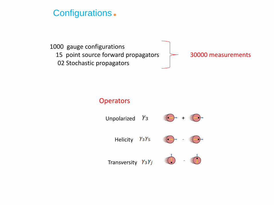
Configurations

1000 gauge configurations15 point source forward propagators02 Stochastic propagators

Operators

𝛾3

30000 measurements

Unpolarized

Helicity

Transversity

+