Embed Size (px)
Citation preview

Journal of Applied Geophysics 95 (2013) 135–156
Contents lists available at SciVerse ScienceDirect
Journal of Applied Geophysics
j ourna l homepage: www.e lsev ie r .com/ locate / jappgeo
Recent developments in the direct-current geoelectricalimaging method
M.H. Loke a, J.E. Chambers b, D.F. Rucker c,⁎, O. Kuras b, P.B. Wilkinson b
a Geotomo Software, 115 Cangkat Minden Jalan 6, 11700 Gelugor, Penang, Malaysiab British Geological Survey, Natural Environment Research Council, Kingsley Dunham Centre, Keyworth, Nottingham NG12 5GG, UKc hydroGEOPHYSICS, Inc., 2302 N Forbes Blvd., Tucson AZ 85745, USA
⁎ Corresponding author. Tel.: +1 520 343 5434.E-mail addresses: [email protected] (M.H. Loke
(D.F. Rucker).
0926-9851/$ – see front matter © 2013 Natural Environhttp://dx.doi.org/10.1016/j.jappgeo.2013.02.017
a b s t r a c t
a r t i c l e i n f oArticle history:Received 21 September 2012Accepted 19 February 2013Available online 22 March 2013
Keywords:Electrical resistivityReviewDevelopmentsTomographyApplicationsLimitations
There have been major improvements in instrumentation, field survey design and data inversion techniquesfor the geoelectrical method over the past 25 years. Multi-electrode and multi-channel systems have made itpossible to conduct large 2-D, 3-D and even 4-D surveys efficiently to resolve complex geological structuresthat were not possible with traditional 1-D surveys. Continued developments in computer technology, aswell as fast data inversion techniques and software, have made it possible to carry out the interpretationon commonly available microcomputers. Multi-dimensional geoelectrical surveys are nowwidely used in en-vironmental, engineering, hydrological and mining applications. 3-D surveys play an increasingly importantrole in very complex areas where 2-D models suffer from artifacts due to off-line structures. Large areas onland and water can be surveyed rapidly with computerized dynamic towed resistivity acquisition systems.The use of existing metallic wells as long electrodes has improved the detection of targets in areas wherethey are masked by subsurface infrastructure. A number of PC controlled monitoring systems are also avail-able to measure and detect temporal changes in the subsurface. There have been significant advancements intechniques to automatically generate optimized electrodes array configurations that have better resolutionand depth of investigation than traditional arrays. Other areas of active development include the translationof electrical values into geological parameters such as clay and moisture content, new types of sensors, esti-mation of fluid or ground movement from time-lapse images and joint inversion techniques. In this paper, weinvestigate the recent developments in geoelectrical imaging and provide a brief look into the future of wherethe science may be heading.
© 2013 Natural Environment Research Council and Elsevier BV. All rights reserved.
1. Introduction
The resistivity survey method is one of the oldest and most com-monly used geophysical exploration methods (Reynolds, 2011). It iswidely used in environmental and engineering (Chambers et al.,2006; Dahlin, 2001; Rucker et al., 2010), hydrological (Page, 1968;Wilson et al., 2006), archeological (Griffiths and Barker, 1994; Tsokaset al., 2008) and mineral exploration (Bauman, 2005; Legault et al.,2008; White et al., 2001) surveys. It has been used to image structuresfrom the millimeter scale to kilometers (Linderholm et al., 2008; Storzet al., 2000). Besides surveys on the land surface, it has been used acrossboreholes (Chambers et al., 2003; Daily and Owen, 1991) and in aquaticareas (Loke and Lane, 2004; Rucker et al., 2011b).
Since the first commercial use of the resistivity method in the early1920's (Burger et al., 2006) and right up to the late 1980's, it has beenused essentially as a one-dimensional (1-D) mapping method. However,
ment Research Council and Elsevie
even in moderately complex areas, a 1-D approach is not sufficiently ac-curate. Over the last 25 years, there have been revolutionary improve-ments to the resistivity method where two-dimensional (2-D) surveysare now routinely conducted. Three-dimensional (3-D) surveys arewidely used in areas with complex geology, while there have beensignificant interest and developments in four-dimensional (4-D)surveys. This has been made possible by recent developments infield instrumentation, automatic interpretation algorithms, and com-puter software. With the new tools, complex variations of the subsur-face resistivity in both space and time can now be accurately mapped.
In this review, we summarize key developments in the field ofgeoelectrical characterization and monitoring from the past two de-cades. The review is focused more towards the commercial develop-ment of the method, and is complementary to the research orientedreviews presented by Slater (2007) and Revil et al. (2012). It is largelyfocused on the D.C. resistivity method due to space constraints, withreferences to related methods such as induced polarization (I.P.) andspectral I.P. methods where appropriate.
The following section gives a short description of basic principlesof the resistivity method and traditional 1-D resistivity mapping
r BV. All rights reserved.
136 M.H. Loke et al. / Journal of Applied Geophysics 95 (2013) 135–156
methods. This is followed by brief overviews of recent developmentsin 2-D, 3-D and 4-D surveying methods, and practical applications invarious fields. Finally new developments in a few specific areas thatpoint to future trends are described.
2. Basic principles of the resistivity method
The relationship between the electrical resistivity, current and theelectrical potential is governed by Ohm's law. To calculate the poten-tial in a continuous medium, the form of Ohm's Law, combined withthe conservation of current, as given by Poisson's equation is normal-ly used. The potential due to a point current source located at xs isgiven by
∇·1
ρ x; y; zð Þ∇ϕ x; y; zð Þ� �
¼ −∂jc∂t δ xsð Þ ð1Þ
where ρ is the resistivity, ϕ is the potential and jc is the charge density.The potential at any point on the surface or within the medium can becalculated if the resistivity distribution is known. This is the forwardproblem, and we specifically separate it from the inverse problemdiscussed below. For 1-D models (Fig. 1), the forward problem is com-monly solved using the linear filter method (Ghosh, 1971). For 2-Dand 3-D models, analytical methods are used for simple structuressuch as a cylinder or sphere in a homogeneous medium (Wait, 1982;Ward and Hohmann, 1987). Boundary and analytical element methods(Furman et al., 2002; Spiegel et al., 1980; Xu, 2001) can also be used formore general structures but are usually limited to models where thesubsurface is divided into a relatively small number of regions. Formodeling offield data, thefinite-difference and associatedfinite volumemethods (Dey and Morrison, 1979a,b; Pidlisecky et al., 2007), and thefinite-element (Coggon, 1971; Holcombe and Jiracek, 1984) methodare more commonly used. These methods discretize the subsurfaceinto a large number of cells. By using a sufficiently fine mesh and theproper boundary conditions, an accurate solution for the potentialover complex distributions of resistivity can be obtained. In areaswhere anisotropy is significant (LaBrecque and Casale, 2002), Eq. (1)is modified where the resistivity is a vector that includes directionaldependent values instead of a scalar function.
The purpose of the resistivity method is to calculate the electricalresistivity of the subsurface, which is an unknown quantity. Themeasurements for the resistivity survey are made by passing a cur-rent into the ground through two current electrodes (usually metalstakes), and measuring the difference in the resulting voltage at twopotential electrodes. In its most basic form, the resistivity meter hasa current source and voltage measuring circuitry that are connectedby cables to a minimum of four electrodes. The basic data from a
Fig. 1. Resistivity sounding (A) and best-fit three-layer model interpretation (B) for a san(32 Ω.m); middle layer, river terrace sand and gravel (205 Ω.m); lower layer, Oxford Clay
resistivity survey are the positions of the current and potentialelectrodes, the current (I) injected into the ground and the resultingvoltage difference (ΔV) between the potential electrodes (Fig. 2).The current and voltage measurements are then converted into anapparent resistivity (ρa) value by using the following formula
ρa ¼ kΔVI
; ð2Þ
where k is the geometric factor that depends on the configuration of thecurrent and potential electrodes (Koefoed, 1979). Eq. (2) represents thesimplest form of the inverse problem and assumes that the earth is ho-mogeneous for each combination of current and potential measure-ments. Different arrangements of the current and potential electrodes(or arrays) have been devised over the years. The most commonlyused arrays are shown in Fig. 2, along with their associated geometricfactors. The advantages and disadvantages of the different arrays arediscussed in various papers; such as in Dahlin and Zhou (2004),Saydam and Duckworth (1978), Szalai and Szarka (2008) and Zhou etal. (2002). The suitability of an array depends on many factors; amongwhich are its sensitivity to the target of interest, signal-to-noise ratio,depth of investigation, lateral data coverage and more recently the effi-ciency of using it in a multichannel system. The multiple gradient array(Fig. 2F) was designed for use in multi-channel systems (Dahlin andZhou, 2006).
3. Resistivity acquisition, processing and interpretation
3.1. Traditional 1-D resistivity surveys
From the 1920's to the late 1980's there were essentially twosurveying techniques used, the profiling and sounding methods. In aprofiling survey, the distances between the electrodes were kept fixedand the four electrodes were moved along the survey line. A relatedtechnique is the mise-a-la-masse method where one electrode isembedded into a conductive body (with the second current electrodeat a sufficiently far distance) and the potential electrodes are movedaround it to produce an equipotentials map (Parasnis, 1967). The datainterpretation for profiling and mise-a-la-masse surveys were mainlyqualitative. In the sounding method (Koefoed, 1979) the center pointof the electrodes array remained fixed but the spacing between theelectrodes was increased to obtain information about the deeper sec-tions of the subsurface. Usually the Wenner or Schlumberger arrange-ment was used.
The interpretation model consisted of a series of 1-D horizontallayers (Fig. 1A), and the sounding method has been extensivelyused to investigate the ground for resource management, such as
d and gravel reconnaissance survey in the Thames Valley, UK. Note: upper layer, silt(11 Ω.m).

Fig. 2. Some commonly used electrode arrays and their geometric factors. Note that for the multiple gradient array, the total array length is ‘(s + 2)a’ and the distance between thecenter of the potential dipole pair P1–P2 and the center of the current pair C1–C2 is given by ‘ma’.British Geological Survey (c) NERC 2013
137M.H. Loke et al. / Journal of Applied Geophysics 95 (2013) 135–156
mineral, petroleum, and groundwater resources. Initially quantitativeinterpretation of geoelectric sounding data was conducted by usingpre-computed or ‘standard’ sounding curves. Sounding curves werelater superseded by computer inversion techniques with the adventof the linear filter method (Ghosh, 1971; Koefoed, 1979).
The modern application of resistivity processing includes inversemodeling. A commonly used method for sounding data inversion isthe damped least-squares method (Inman, 1975), based on the follow-ing equation:
JTJþ λI� �
Δq ¼ JTΔg; ð3Þ
where, the discrepancy vector Δg contains the difference between thelogarithms of the measured and the calculated apparent resistivityvalues and Δq is a vector consisting of the deviation of the estimatedmodel parameters from the true model. Here, the model parametersare the logarithms of the resistivity and thickness of the model layers.J is the Jacobian matrix of partial derivatives of apparent resistivitywith respect to the model parameters. λ is a damping or regularizationfactor that stabilizes the ill-condition Jacobian matrix usually encoun-tered for geophysical problems. Starting from an initial model (such asa homogeneous earth model), this method iteratively refines themodel so as to reduce the data misfit to a desired level (usually lessthan 5%). Other methods such as the conjugate gradient method, SVDanalysis and global optimization methods (including neural networksand simulated annealing) have also been used for resistivity data inver-sion (Pellerin and Wannamaker, 2005). Fig. 1 shows an example of theresults from a resistivity sounding survey using the offsetWenner array(Barker, 1981) that has a three-layer inversion model.
The main weakness of the sounding method is the assumptionthat there are no lateral changes in the resistivity. It is use-ful in geological situations where this is approximately true, butgives inaccurate results where there are significant lateral changes.The effect of lateral variations on the sounding data can be re-duced by using the offset Wenner method (Barker, 1981) but formore accurate results the lateral changes must be directly incorpo-rated into the interpretation model. It should be noted that someearly combined sounding and profiling surveys to produce 2-Dpseudosections were carried out for mineral exploration (Ward,1990), usually together with I.P. measurements. Conducting thesurveys and quantitative modeling using manual adjustments of aforward model (Hohmann, 1982) was laborious and thus suchsurveys were comparatively rare.
3.2. Multi-electrode systems and 2-D imaging surveys
While the resistivity meter used in sounding and profiling surveystypically has four electrodes connected via four separate cables,a multi-electrode system has 25 or more electrodes connected tothe resistivity meter via a multi-core cable (Fig. 3). Commercialmulti-electrode systems first appeared in the late 1980's (Griffithset al., 1990) and since then have become a standard tool in many geo-physical organizations. An internal switching circuitry controlled by aprogrammable microcomputer or microprocessor within the resistiv-ity meter automatically selects the appropriate 4 electrodes for eachmeasurement. This enables almost any array configuration to beused. By making measurements with different spacings at differentlocations along the cable, a 2-D profile of the subsurface is obtained.Together with the parallel development of fast and stable automaticdata inversion techniques (deGroot-Hedlin and Constable, 1990;
Fig. 3. Schematic diagram of a multi-electrode system, and a possible sequence of measurements to create a 2-D pseudosection.British Geological Survey (c) NERC 2013
138 M.H. Loke et al. / Journal of Applied Geophysics 95 (2013) 135–156
Li and Oldenburg, 1992; Loke and Barker, 1996a) that could beimplemented on commonly available microcomputers, 2-D electricalimaging surveys became widely used in the early 1990's.
A 2-D model that consists of a large number of rectangular cellsis commonly used to interpret the data (Loke and Barker, 1996a).The resistivity of the cells is allowed to vary in the vertical and onehorizontal direction, but the size and position of the cells are fixed.Again, different numerical methods can be used to calculate thepotential values for the 2-D forward model. Inverse methods arethen used to back calculate the resistivity that gave rise to the mea-sured potential measurements. Starting from a simple initial model(usually a homogeneous half-space), an optimization method isused to iteratively change the resistivity of the model cells to mini-mize the difference between the measured and calculated apparentresistivity values. The inversion problem is frequently ill-posedand ill-constrained due to incomplete, inconsistent and noisy data.Smoothness or other constraints are usually incorporated to stabilizethe inversion procedure to avoid numerical artifacts. As an example,the following equation includes a model smoothness constraint tothe least-squares optimization method,
JTJþ λF� �
Δqk ¼ JTΔgk−λFqk−1; ð4Þ
where
F ¼ αxCTxCx þ αzC
TzCz: ð5Þ
Cx and Cz are the roughness filter matrices in the horizontal (x)and vertical (z) directions and αx and αz are the respective relativeweights of the roughness filters. k represents the iteration number.One common form of the roughness filter is the first-order differencematrix (deGroot-Hedlin and Constable, 1990), but the elements ofthe matrices can be modified to introduce other desired character-istics into the inversion model (Farquharson, 2008; Pellerin andWannamaker, 2005). An L1-norm criterion can be used to produce‘blocky’ models for regions that are piecewise constant and separatedby sharp boundaries (Farquharson and Oldenburg, 1998; Loke et al.,
2003). The laterally constrained inversion method (Auken andChristiansen, 2004) that includes sharp boundaries has been success-fully used in areas with a layered subsurface structure. Joint inversionalgorithms using other geophysical or geological data to constrain themodel have also been implemented to help produce models that areconsistent with known information (Bouchedda et al., 2012; Hinnellet al., 2010; Linde et al., 2006a). A number of micro-computer basedsoftware are now available that can automatically carry out the inver-sion of a 2-D survey data set in a very short period of time.
There are many commercial multi-electrode resistivity systemscapable of connecting up to several hundreds of electrodes at once,with electrode spacings practically varying from 1 to 20 m. A recentdevelopment over the past 10 years is multi-channeled systemsthat can greatly reduce the survey time. Only two electrodes can beused as the current electrodes at a single time, but the voltagemeasurements can be made between many different pairs of poten-tial electrodes. Commercial systems with 4 to 10 channels are widelyavailable, and some customized systems have more than 100channels (Rucker et al., in press; Stummer et al., 2002). New dataacquisition techniques, such as using the multiple gradient array(Dahlin and Zhou, 2006), have been designed for the multi-channeled systems.
Fig. 4A shows an apparent resistivity pseudosection from a surveyusing the dipole–dipole array to map shallow Quaternary deposits atthe Eddleston experimental site, Scottish Borders, UK (Dochartaighet al., 2011). The dipole–dipole array was used with the dipole length‘a’ ranging from 3 to 18 m, and the dipole separation factor ‘n’ rangingfrom 1 to 8. The mid-point of the array was used to set the horizontallocation of the plotting point in the pseudosection, while the ‘mediandepth of investigation’ method was used to calculate the verticalposition (Edwards, 1977). The southern (left) half of the line lies ina floodplain where it crosses a small stream, while the northern(right) half crosses over into grasslands above the floodplain. Therelatively flat southern section is characterized by a low resistivitytop layer consisting of present-day alluvial deposits, with a generalincrease in the resistivity towards the northern end located on slightlyelevated grasslands (Fig. 4B). The higher resistivity layer at a depth of5 to 15 m corresponds to a coarser alluvial layer with some gravels.
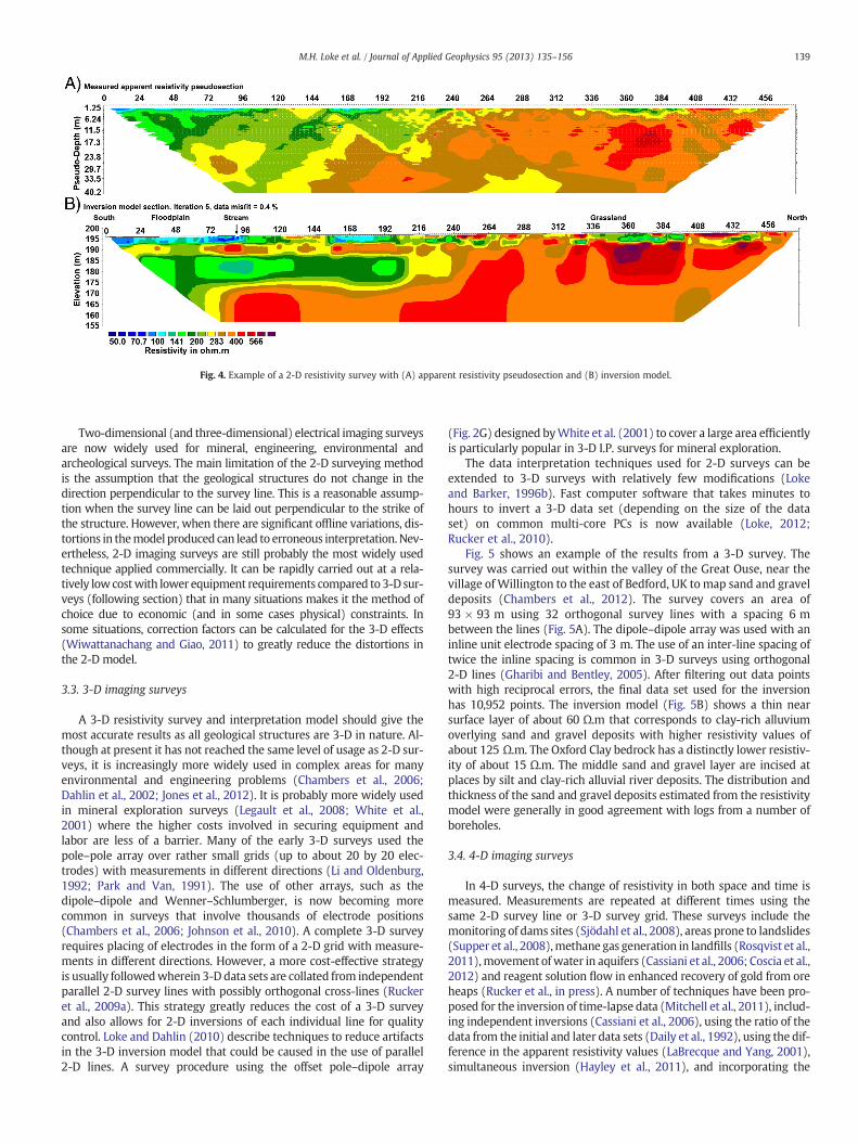
Fig. 4. Example of a 2-D resistivity survey with (A) apparent resistivity pseudosection and (B) inversion model.
139M.H. Loke et al. / Journal of Applied Geophysics 95 (2013) 135–156
Two-dimensional (and three-dimensional) electrical imaging surveysare now widely used for mineral, engineering, environmental andarcheological surveys. The main limitation of the 2-D surveying methodis the assumption that the geological structures do not change in thedirection perpendicular to the survey line. This is a reasonable assump-tion when the survey line can be laid out perpendicular to the strike ofthe structure. However, when there are significant offline variations, dis-tortions in themodel produced can lead to erroneous interpretation. Nev-ertheless, 2-D imaging surveys are still probably the most widely usedtechnique applied commercially. It can be rapidly carried out at a rela-tively lowcostwith lower equipment requirements compared to 3-D sur-veys (following section) that in many situations makes it the method ofchoice due to economic (and in some cases physical) constraints. Insome situations, correction factors can be calculated for the 3-D effects(Wiwattanachang and Giao, 2011) to greatly reduce the distortions inthe 2-D model.
3.3. 3-D imaging surveys
A 3-D resistivity survey and interpretation model should give themost accurate results as all geological structures are 3-D in nature. Al-though at present it has not reached the same level of usage as 2-D sur-veys, it is increasingly more widely used in complex areas for manyenvironmental and engineering problems (Chambers et al., 2006;Dahlin et al., 2002; Jones et al., 2012). It is probably more widely usedin mineral exploration surveys (Legault et al., 2008; White et al.,2001) where the higher costs involved in securing equipment andlabor are less of a barrier. Many of the early 3-D surveys used thepole–pole array over rather small grids (up to about 20 by 20 elec-trodes) with measurements in different directions (Li and Oldenburg,1992; Park and Van, 1991). The use of other arrays, such as thedipole–dipole and Wenner–Schlumberger, is now becoming morecommon in surveys that involve thousands of electrode positions(Chambers et al., 2006; Johnson et al., 2010). A complete 3-D surveyrequires placing of electrodes in the form of a 2-D grid with measure-ments in different directions. However, a more cost-effective strategyis usually followedwherein 3-D data sets are collated from independentparallel 2-D survey lines with possibly orthogonal cross-lines (Ruckeret al., 2009a). This strategy greatly reduces the cost of a 3-D surveyand also allows for 2-D inversions of each individual line for qualitycontrol. Loke and Dahlin (2010) describe techniques to reduce artifactsin the 3-D inversion model that could be caused in the use of parallel2-D lines. A survey procedure using the offset pole–dipole array
(Fig. 2G) designed byWhite et al. (2001) to cover a large area efficientlyis particularly popular in 3-D I.P. surveys for mineral exploration.
The data interpretation techniques used for 2-D surveys can beextended to 3-D surveys with relatively few modifications (Lokeand Barker, 1996b). Fast computer software that takes minutes tohours to invert a 3-D data set (depending on the size of the dataset) on common multi-core PCs is now available (Loke, 2012;Rucker et al., 2010).
Fig. 5 shows an example of the results from a 3-D survey. Thesurvey was carried out within the valley of the Great Ouse, near thevillage of Willington to the east of Bedford, UK to map sand and graveldeposits (Chambers et al., 2012). The survey covers an area of93 × 93 m using 32 orthogonal survey lines with a spacing 6 mbetween the lines (Fig. 5A). The dipole–dipole array was used with aninline unit electrode spacing of 3 m. The use of an inter-line spacing oftwice the inline spacing is common in 3-D surveys using orthogonal2-D lines (Gharibi and Bentley, 2005). After filtering out data pointswith high reciprocal errors, the final data set used for the inversionhas 10,952 points. The inversion model (Fig. 5B) shows a thin nearsurface layer of about 60 Ω.m that corresponds to clay-rich alluviumoverlying sand and gravel deposits with higher resistivity values ofabout 125 Ω.m. The Oxford Clay bedrock has a distinctly lower resistiv-ity of about 15 Ω.m. The middle sand and gravel layer are incised atplaces by silt and clay-rich alluvial river deposits. The distribution andthickness of the sand and gravel deposits estimated from the resistivitymodel were generally in good agreement with logs from a number ofboreholes.
3.4. 4-D imaging surveys
In 4-D surveys, the change of resistivity in both space and time ismeasured. Measurements are repeated at different times using thesame 2-D survey line or 3-D survey grid. These surveys include themonitoring of dams sites (Sjödahl et al., 2008), areas prone to landslides(Supper et al., 2008),methane gas generation in landfills (Rosqvist et al.,2011),movement ofwater in aquifers (Cassiani et al., 2006; Coscia et al.,2012) and reagent solution flow in enhanced recovery of gold from oreheaps (Rucker et al., in press). A number of techniques have been pro-posed for the inversion of time-lapse data (Mitchell et al., 2011), includ-ing independent inversions (Cassiani et al., 2006), using the ratio of thedata from the initial and later data sets (Daily et al., 1992), using the dif-ference in the apparent resistivity values (LaBrecque and Yang, 2001),simultaneous inversion (Hayley et al., 2011), and incorporating the
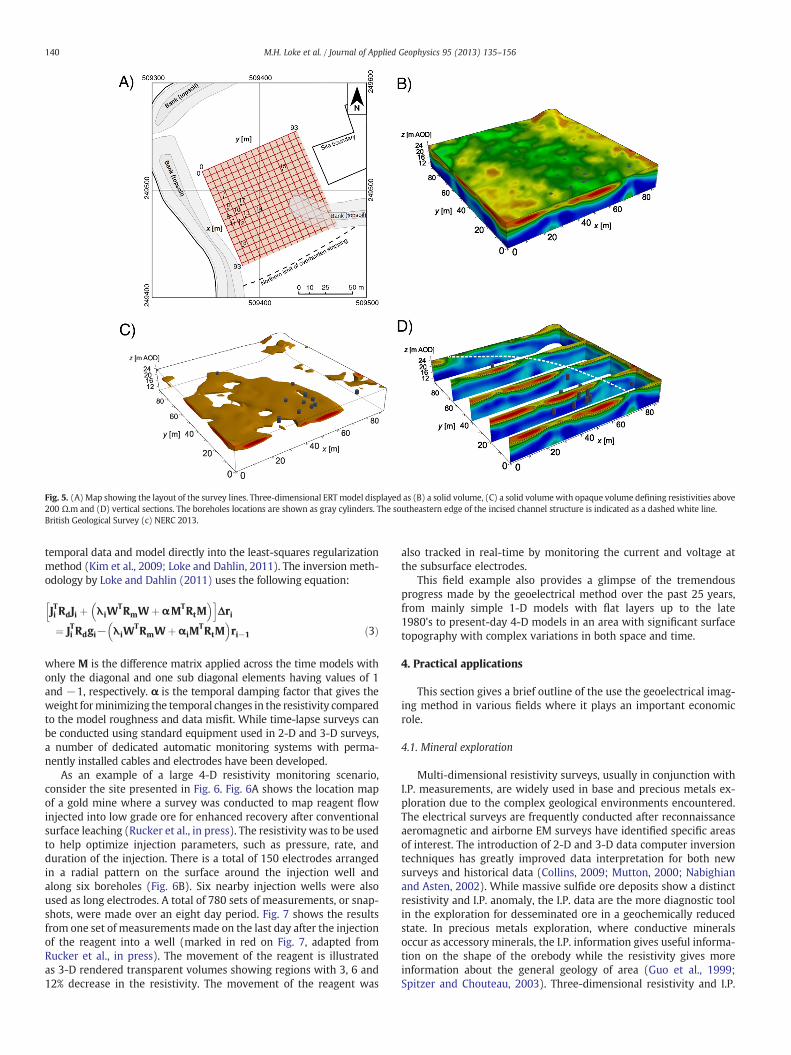
Fig. 5. (A)Map showing the layout of the survey lines. Three-dimensional ERT model displayed as (B) a solid volume, (C) a solid volumewith opaque volume defining resistivities above200 Ω.m and (D) vertical sections. The boreholes locations are shown as gray cylinders. The southeastern edge of the incised channel structure is indicated as a dashed white line.British Geological Survey (c) NERC 2013.
140 M.H. Loke et al. / Journal of Applied Geophysics 95 (2013) 135–156
temporal data and model directly into the least-squares regularizationmethod (Kim et al., 2009; Loke and Dahlin, 2011). The inversion meth-odology by Loke and Dahlin (2011) uses the following equation:
JTi RdJi þ λiWTRmW þ αMTRtM
� �h iΔri
¼ JTi Rdgi− λiWTRmW þ αiM
TRtM� �
ri−1 ð3Þ
where M is the difference matrix applied across the time models withonly the diagonal and one sub diagonal elements having values of 1and −1, respectively. α is the temporal damping factor that gives theweight forminimizing the temporal changes in the resistivity comparedto the model roughness and data misfit. While time-lapse surveys canbe conducted using standard equipment used in 2-D and 3-D surveys,a number of dedicated automatic monitoring systems with perma-nently installed cables and electrodes have been developed.
As an example of a large 4-D resistivity monitoring scenario,consider the site presented in Fig. 6. Fig. 6A shows the location mapof a gold mine where a survey was conducted to map reagent flowinjected into low grade ore for enhanced recovery after conventionalsurface leaching (Rucker et al., in press). The resistivity was to be usedto help optimize injection parameters, such as pressure, rate, andduration of the injection. There is a total of 150 electrodes arrangedin a radial pattern on the surface around the injection well andalong six boreholes (Fig. 6B). Six nearby injection wells were alsoused as long electrodes. A total of 780 sets of measurements, or snap-shots, were made over an eight day period. Fig. 7 shows the resultsfrom one set of measurements made on the last day after the injectionof the reagent into a well (marked in red on Fig. 7, adapted fromRucker et al., in press). The movement of the reagent is illustratedas 3-D rendered transparent volumes showing regions with 3, 6 and12% decrease in the resistivity. The movement of the reagent was
also tracked in real-time by monitoring the current and voltage atthe subsurface electrodes.
This field example also provides a glimpse of the tremendousprogress made by the geoelectrical method over the past 25 years,from mainly simple 1-D models with flat layers up to the late1980's to present-day 4-D models in an area with significant surfacetopography with complex variations in both space and time.
4. Practical applications
This section gives a brief outline of the use the geoelectrical imag-ing method in various fields where it plays an important economicrole.
4.1. Mineral exploration
Multi-dimensional resistivity surveys, usually in conjunction withI.P. measurements, are widely used in base and precious metals ex-ploration due to the complex geological environments encountered.The electrical surveys are frequently conducted after reconnaissanceaeromagnetic and airborne EM surveys have identified specific areasof interest. The introduction of 2-D and 3-D data computer inversiontechniques has greatly improved data interpretation for both newsurveys and historical data (Collins, 2009; Mutton, 2000; Nabighianand Asten, 2002). While massive sulfide ore deposits show a distinctresistivity and I.P. anomaly, the I.P. data are the more diagnostic toolin the exploration for desseminated ore in a geochemically reducedstate. In precious metals exploration, where conductive mineralsoccur as accessory minerals, the I.P. information gives useful informa-tion on the shape of the orebody while the resistivity gives moreinformation about the general geology of area (Guo et al., 1999;Spitzer and Chouteau, 2003). Three-dimensional resistivity and I.P.
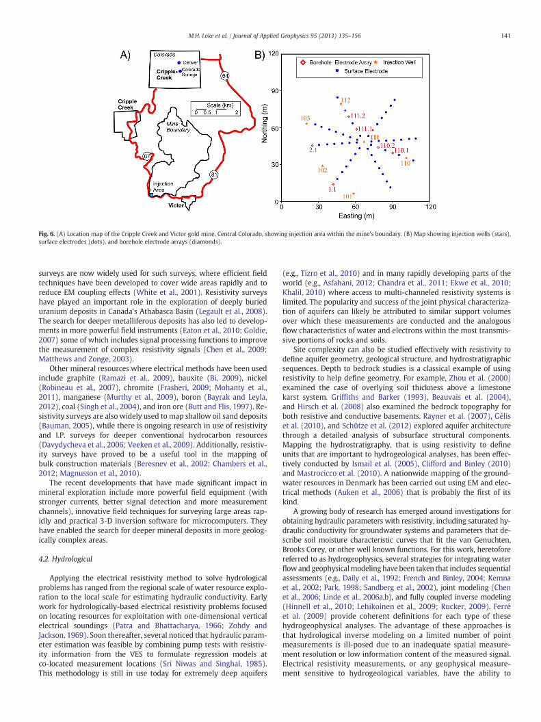
Fig. 6. (A) Location map of the Cripple Creek and Victor gold mine, Central Colorado, showing injection area within the mine's boundary. (B) Map showing injection wells (stars),surface electrodes (dots), and borehole electrode arrays (diamonds).
141M.H. Loke et al. / Journal of Applied Geophysics 95 (2013) 135–156
surveys are now widely used for such surveys, where efficient fieldtechniques have been developed to cover wide areas rapidly and toreduce EM coupling effects (White et al., 2001). Resistivity surveyshave played an important role in the exploration of deeply burieduranium deposits in Canada's Athabasca Basin (Legault et al., 2008).The search for deeper metalliferous deposits has also led to develop-ments in more powerful field instruments (Eaton et al., 2010; Goldie,2007) some of which includes signal processing functions to improvethe measurement of complex resistivity signals (Chen et al., 2009;Matthews and Zonge, 2003).
Other mineral resources where electrical methods have been usedinclude graphite (Ramazi et al., 2009), bauxite (Bi, 2009), nickel(Robineau et al., 2007), chromite (Frasheri, 2009; Mohanty et al.,2011), manganese (Murthy et al., 2009), boron (Bayrak and Leyla,2012), coal (Singh et al., 2004), and iron ore (Butt and Flis, 1997). Re-sistivity surveys are also widely used to map shallow oil sand deposits(Bauman, 2005), while there is ongoing research in use of resistivityand I.P. surveys for deeper conventional hydrocarbon resources(Davydycheva et al., 2006; Veeken et al., 2009). Additionally, resistiv-ity surveys have proved to be a useful tool in the mapping ofbulk construction materials (Beresnev et al., 2002; Chambers et al.,2012; Magnusson et al., 2010).
The recent developments that have made significant impact inmineral exploration include more powerful field equipment (withstronger currents, better signal detection and more measurementchannels), innovative field techniques for surveying large areas rap-idly and practical 3-D inversion software for microcomputers. Theyhave enabled the search for deeper mineral deposits in more geolog-ically complex areas.
4.2. Hydrological
Applying the electrical resistivity method to solve hydrologicalproblems has ranged from the regional scale of water resource explo-ration to the local scale for estimating hydraulic conductivity. Earlywork for hydrologically-based electrical resistivity problems focusedon locating resources for exploitation with one-dimensional verticalelectrical soundings (Patra and Bhattacharya, 1966; Zohdy andJackson, 1969). Soon thereafter, several noticed that hydraulic param-eter estimation was feasible by combining pump tests with resistiv-ity information from the VES to formulate regression models atco-located measurement locations (Sri Niwas and Singhal, 1985).This methodology is still in use today for extremely deep aquifers
(e.g., Tizro et al., 2010) and in many rapidly developing parts of theworld (e.g., Asfahani, 2012; Chandra et al., 2011; Ekwe et al., 2010;Khalil, 2010) where access to multi-channeled resistivity systems islimited. The popularity and success of the joint physical characteriza-tion of aquifers can likely be attributed to similar support volumesover which these measurements are conducted and the analogousflow characteristics of water and electrons within the most transmis-sive portions of rocks and soils.
Site complexity can also be studied effectively with resistivity todefine aquifer geometry, geological structure, and hydrostratigraphicsequences. Depth to bedrock studies is a classical example of usingresistivity to help define geometry. For example, Zhou et al. (2000)examined the case of overlying soil thickness above a limestonekarst system. Griffiths and Barker (1993), Beauvais et al. (2004),and Hirsch et al. (2008) also examined the bedrock topography forboth resistive and conductive basements. Rayner et al. (2007), Géliset al. (2010), and Schütze et al. (2012) explored aquifer architecturethrough a detailed analysis of subsurface structural components.Mapping the hydrostratigraphy, that is using resistivity to defineunits that are important to hydrogeological analyses, has been effec-tively conducted by Ismail et al. (2005), Clifford and Binley (2010)and Mastrocicco et al. (2010). A nationwide mapping of the ground-water resources in Denmark has been carried out using EM and elec-trical methods (Auken et al., 2006) that is probably the first of itskind.
A growing body of research has emerged around investigations forobtaining hydraulic parameters with resistivity, including saturated hy-draulic conductivity for groundwater systems and parameters that de-scribe soil moisture characteristic curves that fit the van Genuchten,Brooks Corey, or other well known functions. For this work, heretoforereferred to as hydrogeophysics, several strategies for integrating waterflowand geophysicalmodelinghave been taken that includes sequentialassessments (e.g., Daily et al., 1992; French and Binley, 2004; Kemnaet al., 2002; Park, 1998; Sandberg et al., 2002), joint modeling (Chenet al., 2006; Linde et al., 2006a,b), and fully coupled inverse modeling(Hinnell et al., 2010; Lehikoinen et al., 2009; Rucker, 2009). Ferréet al. (2009) provide coherent definitions for each type of thesehydrogeophysical analyses. The advantage of these approaches isthat hydrological inverse modeling on a limited number of pointmeasurements is ill-posed due to an inadequate spatial measure-ment resolution or low information content of the measured signal.Electrical resistivity measurements, or any geophysical measure-ment sensitive to hydrogeological variables, have the ability to
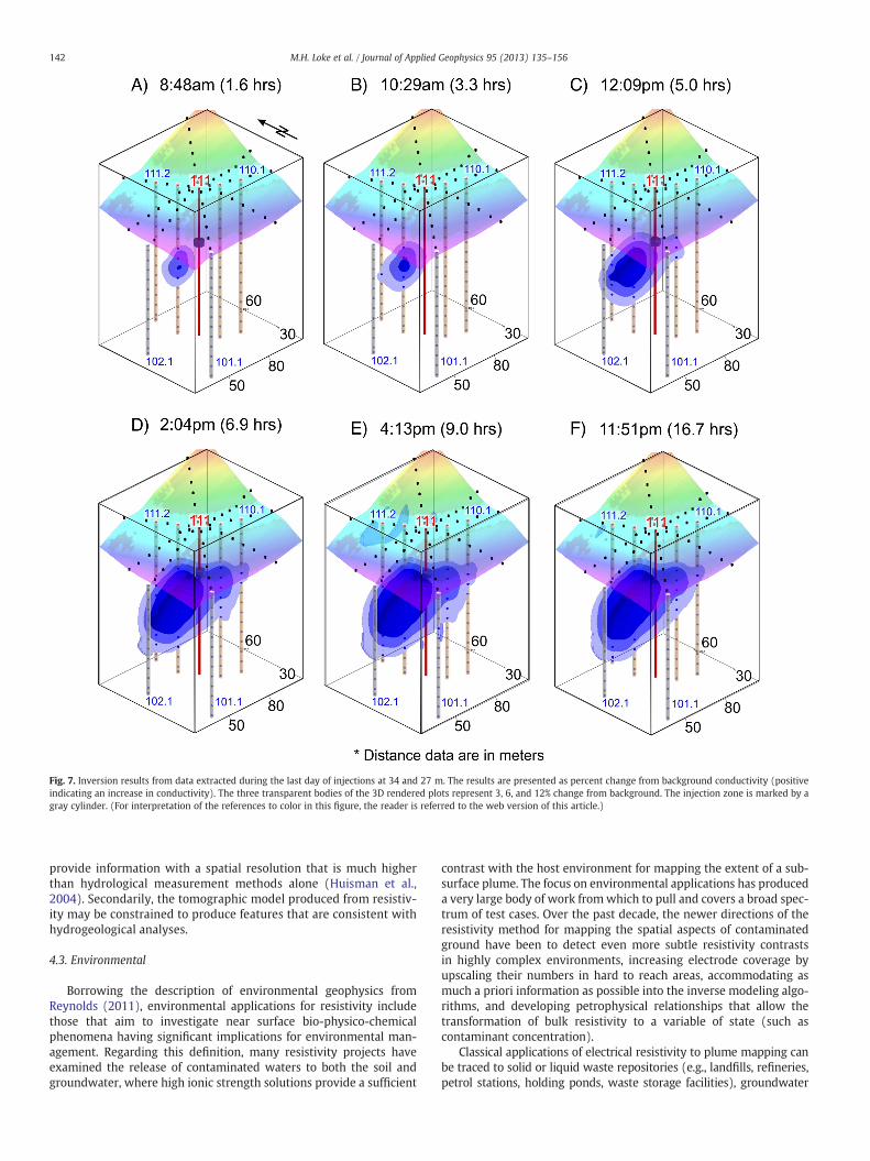
Fig. 7. Inversion results from data extracted during the last day of injections at 34 and 27 m. The results are presented as percent change from background conductivity (positiveindicating an increase in conductivity). The three transparent bodies of the 3D rendered plots represent 3, 6, and 12% change from background. The injection zone is marked by agray cylinder. (For interpretation of the references to color in this figure, the reader is referred to the web version of this article.)
142 M.H. Loke et al. / Journal of Applied Geophysics 95 (2013) 135–156
provide information with a spatial resolution that is much higherthan hydrological measurement methods alone (Huisman et al.,2004). Secondarily, the tomographic model produced from resistiv-ity may be constrained to produce features that are consistent withhydrogeological analyses.
4.3. Environmental
Borrowing the description of environmental geophysics fromReynolds (2011), environmental applications for resistivity includethose that aim to investigate near surface bio-physico-chemicalphenomena having significant implications for environmental man-agement. Regarding this definition, many resistivity projects haveexamined the release of contaminated waters to both the soil andgroundwater, where high ionic strength solutions provide a sufficient
contrast with the host environment for mapping the extent of a sub-surface plume. The focus on environmental applications has produceda very large body of work fromwhich to pull and covers a broad spec-trum of test cases. Over the past decade, the newer directions of theresistivity method for mapping the spatial aspects of contaminatedground have been to detect even more subtle resistivity contrastsin highly complex environments, increasing electrode coverage byupscaling their numbers in hard to reach areas, accommodating asmuch a priori information as possible into the inverse modeling algo-rithms, and developing petrophysical relationships that allow thetransformation of bulk resistivity to a variable of state (such ascontaminant concentration).
Classical applications of electrical resistivity to plume mapping canbe traced to solid or liquid waste repositories (e.g., landfills, refineries,petrol stations, holding ponds, waste storage facilities), groundwater
143M.H. Loke et al. / Journal of Applied Geophysics 95 (2013) 135–156
contamination from salt-laden waters originating from industrial,mining, and agricultural processes (e.g., brine pits, road salt or fertilizerrun off, tailing piles, animal feed lots), and coastal salt water intrusionmapping. Examples for leachate emanating from a landfill are plentifulin the published literature, but a few recent studies include those byBernstone et al. (2000), Chambers et al. (2006), and Clément et al.(2010). Agriculturally based contamination case studies have includednitrate infiltration from nonpoint source releases through the overuseof fertilizers (Boadu et al., 2008) and animal waste at feedlots (Sainatoet al., 2012). Hydrocarbon-based spills have also been shown to beinteresting targets, as a resistive body may develop from free product(Atekwana and Atekwana, 2010) or a conductive body from the degra-dation of chlorinated solvents (Sauck, 2000). Some of the more intensetargets have been discovered around nuclear waste disposal sites(Rucker et al., 2009a) and mine tailings (Martín-Crespo et al., 2011;Rucker et al., 2009b), where ratios of resistivity from background condi-tions to contaminated ground can easily reach 10,000:1. A similar appli-cation with large resistivity contrasts is saline water intrusion mappingin coastal areas (de Franco et al., 2009; Wilson et al., 2006). Severalresearchers have used the resistivity method to examine a reduction incontaminant loading from cleanup activities and remediation (Bentleyand Gharibi, 2004; Chambers et al., 2010; Slater and Binley, 2003).
The examples above discuss environmental applications of resistiv-ity from unplanned releases, whereby contaminants are accidentallyreleased or the consequences of releasewere not meant to be as severe.An alternative realm of study is the planned release of an electrolytictracer tomore fully understand physical and chemical processes withinporous media. Early work by Fried (1975), White (1988), and Lile et al.(1997) used resistivity imaging during salt water injections to under-stand groundwater flow directions, velocities, and mechanical dis-persion. Presently, the practice is quite common in open ground(e.g., Cassiani et al., 2006; Monego et al., 2010; Robert et al., 2012;Wilkinson et al., 2010b) and within small sand tanks and columns(Lekmine et al., 2012; Slater et al., 2002).
The large number of test cases available in the literature is a testa-ment to the versatility of resistivity to solve many different types ofenvironmental problems, from the large catchment scale (Robinsonet al., 2008) to characterization of pore-scale transport processes(Singha et al., 2008). Complex industrial sites also have a particularsubset of novel solutions for acquiring data, including a high densityof borehole arrays (Johnson et al., 2010), push technology (Pidliseckyet al., 2006), and the use of wells as long electrodes (Rucker et al.,2010, 2011a, 2012). Finally, to accommodate all spatial and temporalscales necessary to capture the relevant dynamics of these specializedproblems, both high capacity acquisition hardware (e.g., Kuras et al.,2009; Rucker et al., in press) and software (Loke et al., in press) areavailable to increase the resolution of the method and highlight evenmore subtle features.
4.4. Engineering
Resistivity imaging is widely used across an enormous range ofengineering applications, including the investigation and monitoringof made or artificial ground, and structures such as foundations,tunnels, earthworks and landfills, soil stability, as well as anthropo-genic problems associated with mining related activities.
Spatial information provided by resistivity imaging has proved to beeffective in characterizing heterogeneous made ground, in terms ofthickness and internal and external geometry (Guerin et al., 2004). Forfoundations, it has been applied to pre-installation ground assessment(Soupios et al., 2007), investigation of existing foundations (Cardarelliet al., 2007), and the monitoring of foundation stabilization procedures(Santarato et al., 2011). It has been used to predict ground conditionsahead of tunneling operations (Danielsen and Dahlin, 2009) to differen-tiate between poor (weathered) and good (unweathered) quality rock.Earthwork investigations employing resistivity imaging have been
used to characterize (Bedrosian et al., 2012; Kim et al., 2007; Minsleyet al., 2011; Oh, 2012) and monitor (Sjödahl et al., 2008, 2009, 2010)dams, and assess the condition of rail (Chambers et al., 2008; Donohueet al., 2011) and road (Fortier et al., 2011; Jackson et al., 2002) embank-ments. Mine related engineering applications include in-mine imagingduring working (van Schoor, 2005; van Schoor and Binley, 2010), aswell as the detection and characterization of old abandoned mineworkings (Chambers et al., 2007; Kim et al., 2006; Maillol et al., 1999;Wilkinson et al., 2005, 2006a).
Resistivity imaging is now a well-established technique for land-slide studies (Jongmans and Garambois, 2007), as it provides rapidand lightweight means of acquiring spatial information related toground structure, composition, and hydrogeology on unstable slopes.Landslide investigations are dominated by 2-D resistivity imagingwith numerous recent examples of the use of the technique forstructural characterization in hard-rock settings (Bekler et al., 2011;Jomard et al., 2010; Le Roux et al., 2011; Migon et al., 2010; Paneket al., 2010; Socco et al., 2010; Tric et al., 2010; Zerathe and Lebourg,2012) and soft rock settings (Bievre et al., 2012; Chang et al., 2012;de Bari et al., 2011; Erginal et al., 2009; Grandjean et al., 2011;Hibert et al., 2012; Jongmans et al., 2009; Lebourg et al., 2010;Piegari et al., 2009), and hydrogeological investigations (Bievre et al.,2012; Grandjean et al., 2009; Jomard et al., 2010; Lee et al., 2012;Travelletti et al., 2012; Yamakawa et al., 2010). Three-dimensionalresistivity imaging, while less commonly applied, has also been usedto investigate the internal structure and hydrogeological regimesassociated with landslides (Chambers et al., 2011; Di Maio andPiegari, 2011, 2012; Heincke et al., 2010; Lebourg et al., 2005;Udphuay et al., 2011). A class of landslide hazard for which resistivityimaging has proved to be particularly applicable is quick clay, which isprevalent across parts of Scandinavia and North America. Resistivityimaging has been used to locate and map quick clay formations dueto the higher resistivity exhibited by quick (leached) compared tonon-quick (unleached) formations (Donohue et al., 2012; Lundstromet al., 2009; Solberg et al., 2008, 2012).
A number of studies describe the use of resistivity imaging fordetecting open cavities (Deceuster et al., 2006; Nyquist et al., 2007;Zhu et al., 2012), collapsed or suffused sinkholes (Ezersky, 2008;Gutiérrez et al., 2009; Valois et al., 2011), and caves (Schwartz et al.,2008) that may affect the structural integrity of a building or maypose a safety hazard. As a target, these features can be either conductivefor the water- and clay-filled cavities, or resistive for air-filled cavities(Smith, 1986). Electrical resistivity lines placed either on the surfaceor in boreholes have been used to help find and map these featuresquite successfully.
Others have used resistivity to specifically understand geotechni-cal properties of engineering materials. Unfortunately, there is nodirect causative relationship between electrical resistivity and, say,rock strength. Indirectly, however, the resistivity value can be depen-dent upon jointly influencing parameters that comprise certainhydrogeological (e.g., Boadu, 2011; Boadu and Owusu-Nimo, 2010)or geomechanical attributes of rock, such as porosity, void ratio,water content, cementation, or composition. The Archie equation(Archie, 1942) shows that for fully saturated media, an increase inporosity causes the resistivity to decrease exponentially. In cases ofsedimentary rock, the porosity exponent has been related to cemen-tation or tortuosity through the pore networks (Schon, 1996). Basedon these influencing parameters that link porosity to both elasticmodulus (e.g., Kahraman and Alber, 2006) and electrical resistivity,some have constructed simple correlations between a mechanicalparameter and a resistivity for co-located measurements. This wasthe method applied by Braga et al. (1999), Oh and Sun (2008), andSudha et al. (2009) when presenting blow count from standardpenetration tests to an inverted resistivity value, when acquired asone-dimensional vertical electrical soundings or two-dimensionaltransects. Cosenza et al. (2006) used resistivity to create a scatter
144 M.H. Loke et al. / Journal of Applied Geophysics 95 (2013) 135–156
plot of co-located data with the cone resistance and found logicalgroupings of data associated with the specific lithology from whichthe data were collected.
4.5. Agriculture and soil science
Resistivity, and in particular its reciprocal, electrical conductivity(EC), have played an important role in the fields of agriculture andsoil science for many years as they are among the most useful andeasily obtained spatial properties of soil that influence crop produc-tivity (Corwin and Lesch, 2003, 2005; Samouelian et al., 2005). Thesensitivity of both parameters to soil moisture content, salinity andclay fraction makes them ideal candidates for mapping and evalu-ating the properties of agricultural land, for characterizing fieldvariability in precision agriculture and for monitoring of hydrologicalprocesses and soil performance in terms of nutrient cycling andstorage. Traditionally, high-resolution lateral mapping of resistivityor soil EC at discrete depths of investigation (Dabas, 2009; Dabaset al., 2012; Gebbers et al., 2009) has been favored over resistivityimaging in the strict interpretation of the term, and a range of mea-surement techniques based on inductively, galvanically and capaci-tively coupled sensors is available (Allred et al., 2006; Dabas andTabbagh, 2003).
Direct-current resistivity imaging (2-D and 3-D) has been success-fully applied to characterize the tillage layer (Basso et al., 2010;Besson et al., 2004; Seger et al., 2009), to detect soil cracking at smallscales (Samouelian et al., 2004), to estimate and monitor soil moisturein the root zone and monitor plant uptake (Celano et al., 2011;Nijland et al., 2010; Schwartz et al., 2008), to assess soil water deficit(Brunet et al., 2010), to monitor water percolation and optimize irriga-tion patterns (Greve et al., 2011; Kelly et al., 2011), to map and quantifyroot biomass (al Hagrey, 2007; Amato et al., 2009; Rossi et al., 2011),to characterize soil contamination and monitor remedial treatment(West et al., 1999), to define management zones on farms, plantationsand vineyards (Morari et al., 2009), to investigate soil weatheringprofiles (Beauvais et al., 2004), and to establish integrated 3D soil-geologymodels (Tye et al., 2011). Resistivity imaging is also used exten-sively in the related field of geoforensics (Pringle et al., 2008; Ruffell andMcKinley, 2005).
4.6. Archeology and cultural heritage
In terms of its historical development, the ERT method is arguablyvery closely associated with archeological investigation (Noel and Xu,1991). For archeological purposes however, the lateral mapping ofresistivity (or more typically earth resistance, i.e. the response of afixed-geometry four-electrode array inserted into the soil) has longbeen dominant amongst electrical methods for characterizing largearcheological sites and discriminating buried man-made structures(Gaffney, 2008). More recently though, detailed 2-D and 3-D resistiv-ity imaging have become increasingly popular amongst archeologistsas the method permits closer scrutiny of archeological targets prior toexcavation, for example by volumetric analysis and visualization.
Successful archeological applications of DC resistivity imaging in-clude the non-destructive characterization of mounds and tumuli(Griffiths and Barker, 1994; Papadopoulos et al., 2010; Wake et al.,2012), the investigation of multilayered human settlements (Bergeand Drahor, 2011a,b), the mapping of buried walls, voids and passage-ways (Leucci et al., 2007; Negri and Leucci, 2006; Orfanos andApostolopoulos, 2011), the imagingof ancient citywalls andpreeminentmonuments (Tsokas et al., 2011; Tsourlos and Tsokas, 2011), the detec-tion of tombs and the definition of their geometry (Elwaseif and Slater,2010; Matias et al., 2006), the detection of archeological structuresburied under exceptionally thick soil (Drahor, 2006), the investigationof previously excavated and then backfilled features (Sambuelli et al.,1999), the improved understanding of geological constraints on
archeological sites (Ercoli et al., 2012; Similox-Tohon et al., 2006), andthe comprehension of historic workflows and manufacturing processes(Leopold et al., 2011). Seafloor archeological applications of marineresistivity imaging have also been reported (Passaro, 2010).
A promising field of application is “rescue archeology”, whichcomprises archeological survey and excavation carried out in areasthreatened by, or revealed by, construction or other land develop-ment. This type of archeological investigation must be carried out atspeed; hence resistivity imaging proves to be a useful tool to supportthese surveys (Batayneh, 2011; Loperte et al., 2011). Cultural heritagepreservation is another related field where the benefits of resistivityimaging have been recognized (Mol and Preston, 2010). Its use hasbeen frequently reported for the structural assessment and resto-ration of historical buildings built over more ancient structures(Capizzi et al., 2012; Dabas et al., 2000; Di Maio et al., 2012; Tsokaset al., 2008).
4.7. Waterborne resistivity
Electrical resistivity investigations applied in marine environ-ments can be traced back to at least the mid-1930s (Schlumbergeret al., 1934) where the method was used to map limestone outcropsin the Caspian Sea and to determine the depth to bedrock in Algiersharbor (Corwin et al., 1985). Since then, applications for waterborneresistivity have spanned a wide array of problems that mostlymimic terrestrial applications, but with a few that are unique to themarine setting. For example, geological mapping, including bedrockgeometry, structure, lithology, and hydrostratigraphy is a rathertypical application of both land and waterborne resistivity methods(e.g. Rinaldi et al., 2006; Rucker et al., 2011b). Submarine groundwa-ter discharge (SGD), on the other hand, is a particular area of study foroff-shore resistivity characterization. SGD describes how freshwatermay move from aquifers to the sea and several large scale projectshave been conducted to observe these interactions (Day-Lewiset al., 2006; Henderson et al., 2010; Swarzenski et al., 2006, 2007).
The acquisition of resistivity in aquatic environments can beconducted at the water surface with floating electrodes (e.g. Hatchet al., 2010; Kelly et al., 2009; Song and Cho, 2009) or submerged atthe floor (Toran et al., 2010), with both strategies typically used inconjunction with continuous resistivity profiling (CRP). CRP involvestowing a multi-cored cable behind a vessel and using one pair of cur-rent transmitting electrodes and multiple pairs of potential measure-ment electrodes. The rate at which data are acquired is usually slowerfor the submerged array (Corwin et al., 1985), but typical acquisitionrates may be 3–5 km/h (see Snyder andWightman, 2002). The choiceof floating or submerged electrodes depends on the depth of thewater column, with very thin or very thick water columns using sub-merged electrodes and the intermediate range opting for floatingelectrodes. Loke and Lane (2004) recommend that floating electrodesbe used when the water column is no greater than 25% of the totaldepth of investigation and Lagabrielle (1983) discusses the sensitivityof both cases. In extremely shallow situations involving streams, itmay be more advantageous to use fixed submerged arrays insteadof CRP to avoid damage to the cable.
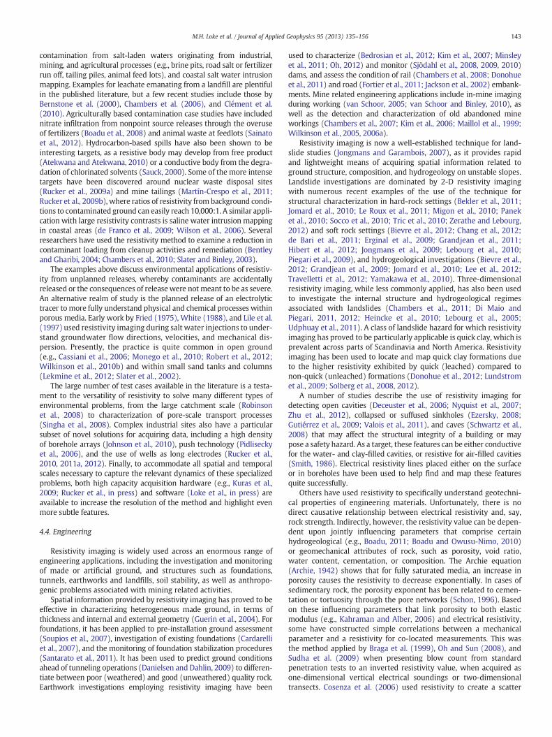
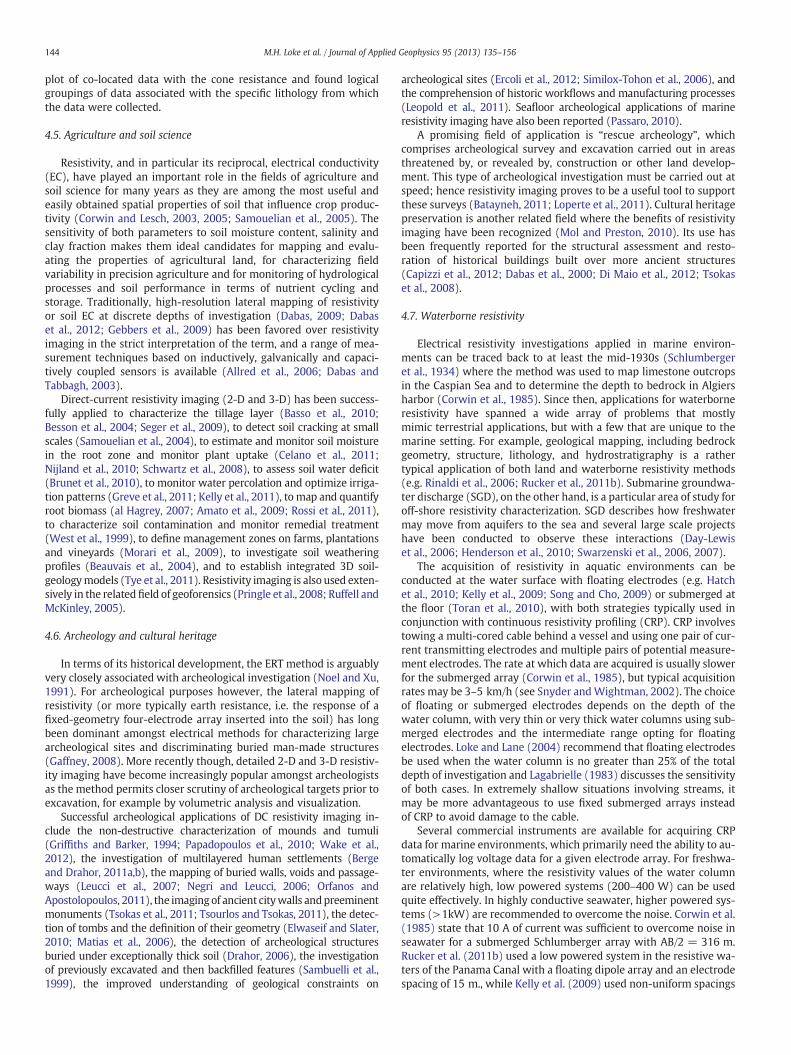
Several commercial instruments are available for acquiring CRPdata for marine environments, which primarily need the ability to au-tomatically log voltage data for a given electrode array. For freshwa-ter environments, where the resistivity values of the water columnare relatively high, low powered systems (200–400 W) can be usedquite effectively. In highly conductive seawater, higher powered sys-tems (>1kW) are recommended to overcome the noise. Corwin et al.(1985) state that 10 A of current was sufficient to overcome noise inseawater for a submerged Schlumberger array with AB/2 = 316 m.Rucker et al. (2011b) used a low powered system in the resistive wa-ters of the Panama Canal with a floating dipole array and an electrodespacing of 15 m., while Kelly et al. (2009) used non-uniform spacings

145M.H. Loke et al. / Journal of Applied Geophysics 95 (2013) 135–156
ranging 0.5 to 128 m. in a survey along the Namoi River in Australia.Butler (2009) lists other examples of instrumentation power versus elec-trode geometry and environment. Most modern equipment also has theability to accept GPS data to help georeference each measurement.
Data processing of the resistivity profiles typically involvestwo-dimensional inversion and investigating conductive or resistivebodies along the transect. Constraints, such as the bathymetry andconductivity of the water, can be added to the inversion to helpresolve issues at the water–rock interface. Provided the data aresufficiently georeferenced, multiple individual profiles can be inter-polated at off-line locations to produce quasi 3-D volumes. Recently,true 3-D inversion models of marine resistivity data collected over aseries of parallel profiles have been generated and Mansoor andSlater (2007) demonstrate how repeated measurements over thesame grid can produce high quality time-lapse information of a shal-low wetland. Rucker and Noonan (in press) demonstrate for longsubparallel lines that 3-D resistivity modeling can still be conductedefficiently if the numerical grid generated for the forward modelis distinctly separate from the inverse model grid. A meandering
Fig. 8. A map showing the Panama Canal survey area (A), the model grid used for the Panamand general geology (B), and the inversion model (C). The first two layers in the inversion msponds to moderately soft tuff, intermediate resistivity to moderately hard agglomerate an
trajectory does not lend itself well to inverse models that strictly ad-here to grids generated from each unique electrode position. Fig. 8presents an example from the survey by Rucker and Noonan(in press) in the Panama canal. Fig. 8A shows the location of the sur-vey and Fig. 8B details the acquisition within the canal as well as thegrid used to conduct the 3D model. Cell sizes were a uniform30 m × 30 m with 2 m layering to a depth of 32 m. The water col-umn ranged from 15 to 19 m with a resistivity of 67 Ω.m. Fig. 8Cshows the results of the inverse 3-D modeling as horizontal slices.The upper two subplots represent the water column and the lowersubplots show the distribution of rock properties associated withhard (high resistivity) or soft (low resistivity) material.
5. Special topics
In this section, a brief overview of more recent developments isgiven. All of the techniques have been tested in field surveys, whilemost are commercially available.
a Canal floating electrodes survey with 20 × 20 m cells together with the survey linesodel correspond to the water column. The lowest resistivity material generally corre-
d high resistivity to hard andesite.
146 M.H. Loke et al. / Journal of Applied Geophysics 95 (2013) 135–156
5.1. Cross-hole ERT
In order to improve the resolution of resistivity images at depth,electrodes are often placed in boreholes (Perri et al., 2012). Measure-ments are then made with various quadripole combinations ofcurrent and potential electrodes, either in the same hole (Slater etal., 2000), between the hole and the surface (Tsourlos et al., 2011)or between pairs of holes (Zhou and Greenhalgh, 2000). The designof surveys for cross-hole imaging has traditionally not been as widelyresearched as for surface investigations, although recent studies havelargely redressed this imbalance. To achieve acceptable image resolu-tion between a pair of boreholes, the separation of the holes shouldnot be more than about 0.75 times the borehole array length(LaBrecque et al., 1996b). The layout of the boreholes can be regular(LaBrecque et al., 1996b; Wilkinson et al., 2006a) or irregular(Chambers et al., 2007; Tsokas et al., 2011) depending on groundconditions and the presence of buildings or infrastructure. Measure-ments are typically made between pairs of boreholes (“panels”) andeither inverted in 2-D for individual panels (Deceuster et al., 2006)or in 3-D for combinations of panels (Nimmer et al., 2008;Wilkinson et al., 2006a). The types and combinations of quadripolesused to measure the data have been studied in terms of maximizingsignal-to-noise and image resolution (al Hagrey, 2011; Goes andMeekes, 2004; Slater et al., 2000; Zhou and Greenhalgh, 2000).Automated survey design algorithms have also been applied to theborehole ERT problem (al Hagrey, 2012; Wilkinson et al., 2006a).Since it is more difficult to determine accurate positions for boreholeelectrodes than surface electrodes, consideration must also be givento the effects of random and systematic offsets in electrode positionsand deviations of the boreholes from their assumed locations anddirection (Oldenborger et al., 2005; Wilkinson et al., 2008; Yi et al.,2009).
Achieving and maintaining good galvanic contact with the groundare also more challenging in boreholes than with surface arrays. Inthe saturated zone, most forms of completion will permit contactwith the electrode, including native backfill (Tsokas et al., 2011),metal casing (Osiensky et al., 2004), and slotted plastic casing(Wilkinson et al., 2006a). In the vadose zone, backfill with bentoniteor similar conductive material is desirable to maintain electrical con-tact (Wilkinson et al., 2010b). However, most forms of completionchange the electrical properties of the ground in the near vicinity ofthe electrodes, and can therefore have a pronounced effect on themeasurements. The effects of metal cased boreholes (Schenkel andMorrison, 1994; Singer and Strack, 1998), grouted boreholes (Deniset al., 2002), and fluid-filled boreholes (Nimmer et al., 2008;Osiensky et al., 2004) have all been analyzed in detail, allowing theeffects of boreholes on the resulting inverted images to be understoodquantitatively. It is further possible to incorporate a borehole modeldirectly in the inversion to remove these effects in 2.5-D (Sugimoto,1999) and 3-D (Doetsch et al., 2010).
5.2. Mobile systems and capacitive resistivity imaging
Continuous data acquisition systems for waterborne surveys weredescribed in an earlier section of this paper. Similar systems for landsurveys have also been developed. Some systems use cylindricalsteel electrodes based on an in-line array geometry (Sørensen,1996), while others use spiked wheels to achieve continuous galvaniccontact with the soil (Dabas, 2009; Panissod et al., 1998). Capacitivelycoupled systems are used in areas with very resistive surfacematerials (e.g. dry or frozen ground) or paved surfaces. These instru-ments use an oscillating, non-grounded electric dipole to generatecurrent flow in the ground and a second similar dipole to measurethe resulting potential distribution at the ground surface (Kuraset al., 2006). There are two major configurations for this type of in-strument. The first configuration (line antenna type) uses cylindrical
transmitters and receivers that are towed behind an operator(Fig. 9A). It gives measurements with typical depths of investigationof 1 to 20 m that are comparable to the galvanically coupled in-linedipole–dipole array (Møller, 2001). However, line antenna data donot fulfill the point source assumption of DC resistivity theory, andparticular care must therefore be taken when interpreting suchdatasets (Neukirch and Klitzsch, 2010). The second type (electrostaticquadripole) uses flatmetallic conductors in an equatorial dipole–dipoleconfiguration (Panissod et al., 1998; Souffache et al., 2010) and hasmaximum survey depths of up to a few meters (Fig. 9B). 2-D and 3-Dsurveys with dense lateral coverage can be rapidly conducted withthese systems, and it has been shown that DC resistivity methodologyand inversion schemes can be usefully applied to such datasets (Kuraset al., 2007). The term “capacitive resistivity imaging (CRI)” has becomesynonymous with this approach. Mobile arrays have traditionallyemployed a limited number of dipoles and associated 2-D and 3-Dmodels are therefore restricted in terms of their spatial resolution.Moreover, these arrays operate primarily at the meter scale. In a morerecent development, Kuras et al. (2012) describe novel multi-sensorCRI instrumentation, which is applied to the 4-D monitoring ofrock-freezing experiments in the laboratory. This methodology holdspromise for applications of ERT in cryospheric science, such as themon-itoring of rocks and soils under permafrost conditions (De Pascale et al.,2008; Hauck and Kneisel, 2006; Krautblatter et al., 2010).
5.3. Unconventional electrodes
Metal stakes are commonly used as the electrodes in resistivitysurveys. While steel electrodes are widely used, other types of metals(and graphite) have also been used (LaBrecque and Daily, 2008; Luand Macnae, 1998). Aluminum foil covered with soil soaked with saltwater is used as current electrodeswhen a current (1 to 20 A) is needed(Ward, 1990). In areas where it is difficult to insert a stake electrode(such as paved ground), flat-base (or plate) electrodes have been used(Athanasiou et al., 2007; Tsokas et al., 2008). Galvanic contact withthe ground is achieved using an electrically conductive gel or mud atthe base of the electrode. Non-polarizable electrodes (Reynolds, 2011)are widely used as the potential electrodes in I.P. surveys to reduce SPnoise, although there has been recent progress in using conventionalmetal electrodes (Dahlin and Leroux, 2012) which aremore convenientto use with multi-electrode systems. In modeling the potentials, theelectrode is usually assumed to be an ideal point. The effect of the finitesize of the electrode is small if the ratio of the electrode length to theelectrode spacing is less than 0.2 (Rücker and Günther, 2011).
In some areas, the existence of widespread subsurface infrastruc-ture can make the detection of subsurface targets by normal surveyswith electrode on the ground surface difficult. The use of existingmetallic wells as long electrodes can significantly improve the detec-tion of targets in such areas (Rucker et al., 2010, 2011a, 2012). Longelectrodes are wells grounded to the earth, extend to the target ofinterest, are already in existence, and can continue to operate in anormal capacity during imaging. Logistically, the wells are connectedto the resistivity acquisition system through a dedicated wire, whichis connected to the inner most casing that extends the deepest intothe earth. Care must be taken to ensure (1) a secured contact betweenthe wire and well, which usually involves cleaning the steel casingwith a wire brush, and (2) the well is electrically isolated fromother metallic infrastructrure such as pipes that may be used tocarry fluid. The numerical models accommodate the long electrodeby assigning those mesh cells representing the well with very lowvalues. Synthetic studies, pilot scale field examples, and full scalefield examples have demonstrated that long electrodes can reproducethe lateral extents of conductive targets with reasonable fidelity, butwith significant loss of vertical resolution. Vertical resolution can beenhanced by combining long electrodes with a large number ofshort electrodes on the surface (Zhu and Feng, 2011), combining
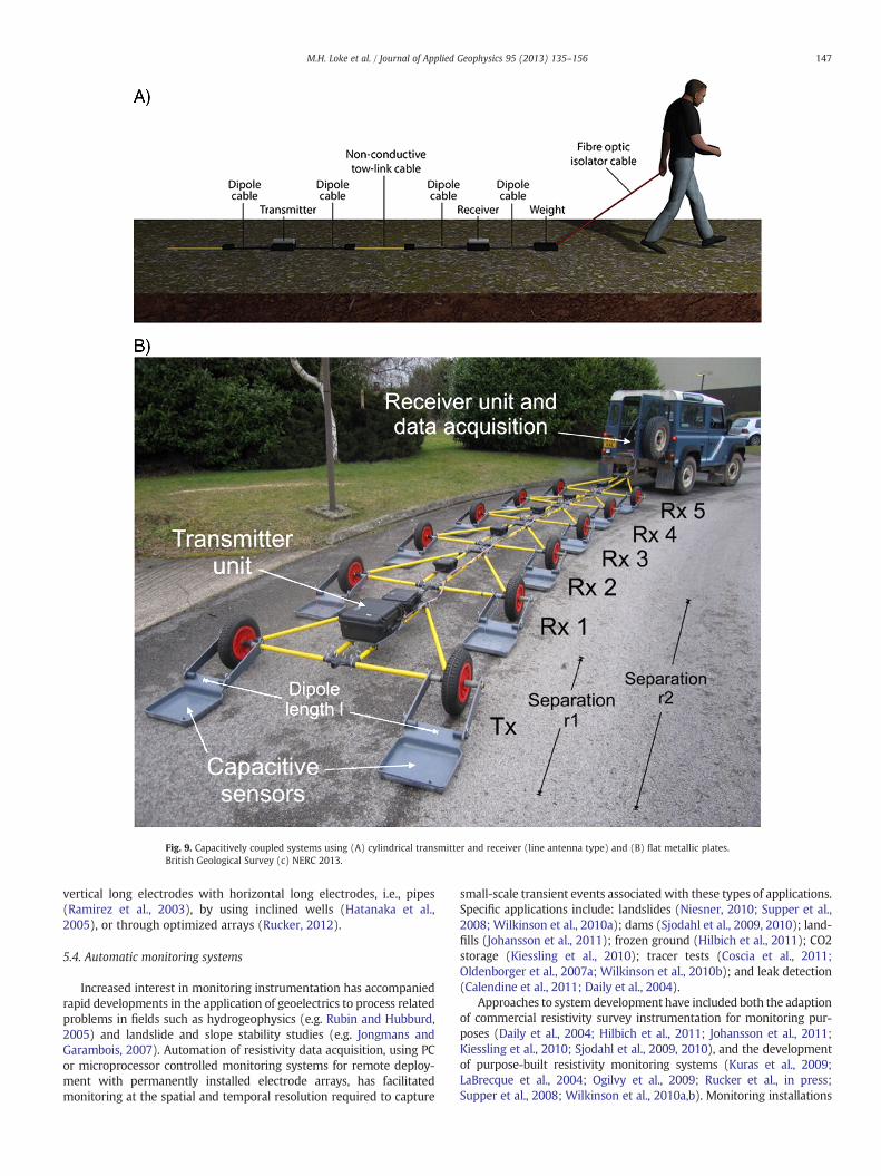
Fig. 9. Capacitively coupled systems using (A) cylindrical transmitter and receiver (line antenna type) and (B) flat metallic plates.British Geological Survey (c) NERC 2013.
147M.H. Loke et al. / Journal of Applied Geophysics 95 (2013) 135–156
vertical long electrodes with horizontal long electrodes, i.e., pipes(Ramirez et al., 2003), by using inclined wells (Hatanaka et al.,2005), or through optimized arrays (Rucker, 2012).
5.4. Automatic monitoring systems
Increased interest in monitoring instrumentation has accompaniedrapid developments in the application of geoelectrics to process relatedproblems in fields such as hydrogeophysics (e.g. Rubin and Hubburd,2005) and landslide and slope stability studies (e.g. Jongmans andGarambois, 2007). Automation of resistivity data acquisition, using PCor microprocessor controlled monitoring systems for remote deploy-ment with permanently installed electrode arrays, has facilitatedmonitoring at the spatial and temporal resolution required to capture
small-scale transient events associated with these types of applications.Specific applications include: landslides (Niesner, 2010; Supper et al.,2008; Wilkinson et al., 2010a); dams (Sjodahl et al., 2009, 2010); land-fills (Johansson et al., 2011); frozen ground (Hilbich et al., 2011); CO2storage (Kiessling et al., 2010); tracer tests (Coscia et al., 2011;Oldenborger et al., 2007a; Wilkinson et al., 2010b); and leak detection(Calendine et al., 2011; Daily et al., 2004).
Approaches to systemdevelopment have included both the adaptionof commercial resistivity survey instrumentation for monitoring pur-poses (Daily et al., 2004; Hilbich et al., 2011; Johansson et al., 2011;Kiessling et al., 2010; Sjodahl et al., 2009, 2010), and the developmentof purpose-built resistivity monitoring systems (Kuras et al., 2009;LaBrecque et al., 2004; Ogilvy et al., 2009; Rucker et al., in press;Supper et al., 2008; Wilkinson et al., 2010a,b). Monitoring installations
148 M.H. Loke et al. / Journal of Applied Geophysics 95 (2013) 135–156
are becoming increasingly sophisticated, and now incorporate telemet-ric control and data transfer, and local power generation through wind,solar, and fuel cell technology (Hilbich et al., 2011; Supper et al., 2008;Wilkinson et al., 2010a). With the automation of data acquisition andthe generation of very large data volumes, systems are also being devel-oped to manage the entire workflow, including scheduling of data col-lection, retrieval and storage, quality assessment and inversion(Chambers et al., in press; LaBrecque et al., 2004; Ogilvy et al., 2009).
5.5. Optimized survey design
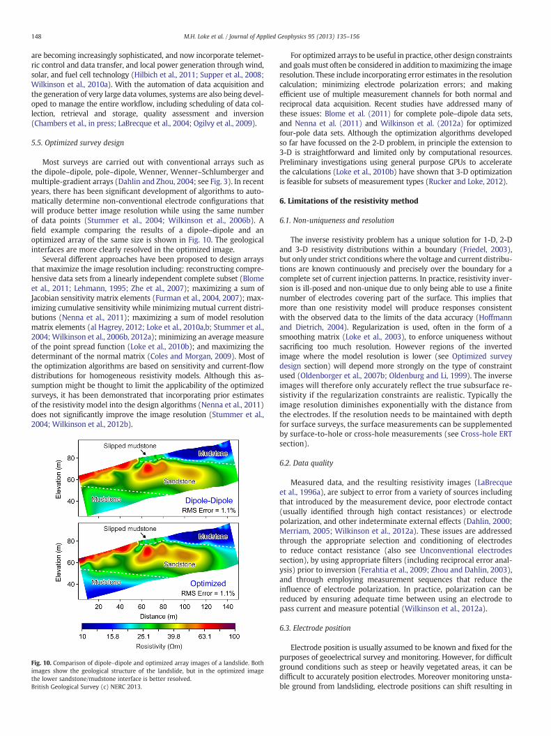
Most surveys are carried out with conventional arrays such asthe dipole–dipole, pole–dipole, Wenner, Wenner–Schlumberger andmultiple-gradient arrays (Dahlin and Zhou, 2004; see Fig. 3). In recentyears, there has been significant development of algorithms to auto-matically determine non-conventional electrode configurations thatwill produce better image resolution while using the same numberof data points (Stummer et al., 2004; Wilkinson et al., 2006b). Afield example comparing the results of a dipole–dipole and anoptimized array of the same size is shown in Fig. 10. The geologicalinterfaces are more clearly resolved in the optimized image.
Several different approaches have been proposed to design arraysthat maximize the image resolution including: reconstructing compre-hensive data sets from a linearly independent complete subset (Blomeet al., 2011; Lehmann, 1995; Zhe et al., 2007); maximizing a sum ofJacobian sensitivity matrix elements (Furman et al., 2004, 2007); max-imizing cumulative sensitivity while minimizing mutual current distri-butions (Nenna et al., 2011); maximizing a sum of model resolutionmatrix elements (al Hagrey, 2012; Loke et al., 2010a,b; Stummer et al.,2004; Wilkinson et al., 2006b, 2012a); minimizing an average measureof the point spread function (Loke et al., 2010b); and maximizing thedeterminant of the normal matrix (Coles and Morgan, 2009). Most ofthe optimization algorithms are based on sensitivity and current-flowdistributions for homogeneous resistivity models. Although this as-sumption might be thought to limit the applicability of the optimizedsurveys, it has been demonstrated that incorporating prior estimatesof the resistivity model into the design algorithms (Nenna et al., 2011)does not significantly improve the image resolution (Stummer et al.,2004; Wilkinson et al., 2012b).
Fig. 10. Comparison of dipole–dipole and optimized array images of a landslide. Bothimages show the geological structure of the landslide, but in the optimized imagethe lower sandstone/mudstone interface is better resolved.British Geological Survey (c) NERC 2013.
For optimized arrays to be useful in practice, other design constraintsand goalsmust often be considered in addition tomaximizing the imageresolution. These include incorporating error estimates in the resolutioncalculation; minimizing electrode polarization errors; and makingefficient use of multiple measurement channels for both normal andreciprocal data acquisition. Recent studies have addressed many ofthese issues: Blome et al. (2011) for complete pole–dipole data sets,and Nenna et al. (2011) and Wilkinson et al. (2012a) for optimizedfour-pole data sets. Although the optimization algorithms developedso far have focussed on the 2-D problem, in principle the extension to3-D is straightforward and limited only by computational resources.Preliminary investigations using general purpose GPUs to acceleratethe calculations (Loke et al., 2010b) have shown that 3-D optimizationis feasible for subsets of measurement types (Rucker and Loke, 2012).
6. Limitations of the resistivity method
6.1. Non-uniqueness and resolution
The inverse resistivity problem has a unique solution for 1-D, 2-Dand 3-D resistivity distributions within a boundary (Friedel, 2003),but only under strict conditionswhere the voltage and current distribu-tions are known continuously and precisely over the boundary for acomplete set of current injection patterns. In practice, resistivity inver-sion is ill-posed and non-unique due to only being able to use a finitenumber of electrodes covering part of the surface. This implies thatmore than one resistivity model will produce responses consistentwith the observed data to the limits of the data accuracy (Hoffmannand Dietrich, 2004). Regularization is used, often in the form of asmoothing matrix (Loke et al., 2003), to enforce uniqueness withoutsacrificing too much resolution. However regions of the invertedimage where the model resolution is lower (see Optimized surveydesign section) will depend more strongly on the type of constraintused (Oldenborger et al., 2007b; Oldenburg and Li, 1999). The inverseimages will therefore only accurately reflect the true subsurface re-sistivity if the regularization constraints are realistic. Typically theimage resolution diminishes exponentially with the distance fromthe electrodes. If the resolution needs to be maintained with depthfor surface surveys, the surface measurements can be supplementedby surface-to-hole or cross-hole measurements (see Cross-hole ERTsection).
6.2. Data quality
Measured data, and the resulting resistivity images (LaBrecqueet al., 1996a), are subject to error from a variety of sources includingthat introduced by the measurement device, poor electrode contact(usually identified through high contact resistances) or electrodepolarization, and other indeterminate external effects (Dahlin, 2000;Merriam, 2005; Wilkinson et al., 2012a). These issues are addressedthrough the appropriate selection and conditioning of electrodesto reduce contact resistance (also see Unconventional electrodessection), by using appropriate filters (including reciprocal error anal-ysis) prior to inversion (Ferahtia et al., 2009; Zhou and Dahlin, 2003),and through employing measurement sequences that reduce theinfluence of electrode polarization. In practice, polarization can bereduced by ensuring adequate time between using an electrode topass current and measure potential (Wilkinson et al., 2012a).
6.3. Electrode position
Electrode position is usually assumed to be known and fixed for thepurposes of geoelectrical survey and monitoring. However, for difficultground conditions such as steep or heavily vegetated areas, it can bedifficult to accurately position electrodes. Moreover monitoring unsta-ble ground from landsliding, electrode positions can shift resulting in
149M.H. Loke et al. / Journal of Applied Geophysics 95 (2013) 135–156
systematic data error which cannot be reduced through reciprocal errorfiltering (Oldenborger et al., 2005; Wilkinson et al., 2008, 2010a; Zhouand Dahlin, 2003). Approaches to reduce the impact of these effectsinclude the selection of measurement array geometries that are lesssensitive to positional errors (Wilkinson et al., 2008), and in the caseof moving electrodes, to estimate electrode position using a positioninversion routine (Wilkinson et al., 2010a).
6.4. Survey design
For very long 2-D survey lines, and for 3-D imaging grids, it can beimpractical to undertake measurements in a single deployment dueto the long cable lengths required. Consequently, very long 2D linesare often surveyed using overlapping sections (e.g. Donohue et al.,2012), and 3-D surface surveys are often undertaken using a networkof lines, where a single line is incrementally migrated across the sur-face to build up a measurement set comprising data from multiplelines (e.g. Bentley and Gharibi, 2004; Dahlin et al., 2002; Ruckeret al., 2009a). Where a single line orientation is used, linear featuresparallel to the line direction can be poorly resolved (Chamberset al., 2002), and banding or herring-bone effects can be present inthe model (Loke and Dahlin, 2010). Mitigation measures include:roll-along (or multiple line) data acquisition methodologies (Dahlinet al., 2002); orthogonal line directions (Chambers et al., 2002;Gharibi and Bentley, 2005); line separations of no more than two elec-trode spacings (Chambers et al., 2002; Gharibi and Bentley, 2005); andappropriate inversion settings (e.g. horizontal diagonal roughnessfilters) (Farquharson, 2008; Loke and Dahlin, 2010).
6.5. Smoothing
Smoothness constrained inversion, which dominates the field ofgeoelectrical imaging, typically produces smoothly varying resistivitydistributions, and so the precise location of geological or engineering in-terfaces can sometimes be difficult to determine in the absence of apriori subsurface information. In addition to robust (L1-norm) inversion(Loke et al., 2003), a range of other interface detection approaches havebeen applied. These include image analysis using gradient-based edgedetectors (Chambers et al., 2012; Elwaseif and Slater, 2010; Hsu et al.,2010), and alternative inversion approaches, such as laterallyconstrained inversion (Wisen et al., 2005), inclusion of sharp bound-aries (Chen et al., 2012; Smith et al., 1999) or joint inversionwith other geophysical data (Bouchedda et al., 2012). In addition,high-contrast heterogeneities in the subsurface that are small com-pared to the model cell-size cannot be accurately modeled, and so canhinder convergence between measured data and the resistivity modelduring the inversion process. However reducing the model cell sizeincreases the computer memory and time required for the data inver-sion, as well as possibly requiring a higher damping constraint to stabi-lize the inversion model (Loke and Dahlin, 2010; Loke and Lane, 2004).From numerical tests with 2-D models, Sasaki (1992) and Loke (2012)showed that using a model cell size of half the unit electrode spacingseems to provide the optimum balance.
6.6. Three-dimensional structures
Off-line three-dimensional structures (including topography) can-not be accurately modeled by 2-D inversion, and so can distortresistivity models (Bentley and Gharibi, 2004; Chambers et al.,2002; Nimmer et al., 2008). These effects can be reduced by ensuringlines are oriented perpendicular to the strike of elongated structuresand by using a 3-D survey approach in complex settings. Although itshould be noted that the edges of 3-D models will also be influencedby 3-D structures outside of the survey area.
6.7. Calibration and interpretation
ERT provides only indirect information of subsurface physical prop-erties such as lithology, moisture content, or temperature, which are ofprincipal interest to geologists, engineers and hydrologists. Due to theoverlapping resistivity ranges of many common earth materials, andthe influence of varying salinity, moisture and temperature, robustinterpretation of resistivity images requires other sources of groundtruth data. For ground investigation, resistivity imaging is routinelyused alongside intrusive methods such as drilling and cone penetrationtesting (CPT) (Wisen et al., 2005). In-situ measurement of resistivity(e.g. CPT resistivity profiles) or laboratory testing of subsurface mate-rials (e.g. Jackson et al., 2006; Russell and Barker, 2010) can be used todirectly constrain the inversion of resistivity data by fixing the resistiv-ities of known regions of the model (e.g. Günther and Rücker, 2009;Pidlisecky et al., 2006). For in-situ or laboratory measurements of resis-tivity to be suitable for constraining inversion, they must provide infor-mation at a scale appropriate to the resolution of the ERTmodel. This isparticularly crucial in highly heterogeneous subsurface conditions. Inthe case of CPT derived resistivitymeasurements, along-profile variabil-ity can be used to determine spatial averaging requirements. Likewise,for laboratory measurements of resistivity, sample volumes and distri-butions representative of the ERT survey resolution and materialheterogeneity are required. Investigation of the relationships betweenresistivity and temperature (Hayley et al., 2007, 2010; Musgrave andBinley, 2011), pore fluid salinity (Hayley et al., 2009; Lekmine et al.,2012; Monego et al., 2010), moisture content (Brunet et al., 2010;Cassiani et al., 2006), and lithology (e.g. Russell and Barker, 2010;Shevnin et al., 2007) are increasingly being undertaken to aid the inter-pretation of ERT sections and time-lapse resistivity monitoring data.
6.8. Anisotropy
The influence of evenmoderately anisotropic media on the results ofresistivity inversion that assumes isotropic conditions can producesignificant distortions in electrical tomograms (e.g. Greenhalgh et al.,2010;Herwanger et al., 2004). Typical geological causes of anisotropy in-clude fracturing, jointing, layering and rock fabric (e.g. strong alignmentof grains slates and shales). Detection of anisotropy has typically beenundertaken using azimuthal (Busby, 2000) and square array (Matias,2008) techniques. However, the most effective approach is perhapssurface to borehole imaging arrays, which unlike surface arrays,are sensitive to anisotropy associated with vertical or sub-vertical axesof symmetry, such as horizontal layering (Greenhalgh et al., 2010). Toaddress the problem of anisotropy, anisotropic resistivity inversionschemes have been developed (Greenhalgh et al., 2009; Herwangeret al., 2004; Kim et al., 2006; Pain et al., 2003); however, these arelimited by number of factors, including the requirement to solve foradditional parameters that exacerbates the problem of non-uniqueness,and the need for subsurface electrodes to effectively detect anisotropyassociated with horizontal layering (Greenhalgh et al., 2010).
7. Conclusions and future trends
There has been tremendous progress in the geoelectrical methodover the last 25 years. The images of the subsurface the methodprovides have become more geologically realistic, from simple 1-Dlayered models to complex 3-D structures varying with time. Therehave been parallel developments in field instrumentation, data inver-sion techniques, and automatic interpretation software that havemade this possible. It is now an established technique widely usedin mineral exploration, environmental, engineering, and hydrologicalsurveys not only on land but also in aquatic regions as well. In thenear future, we foresee an increasingly wider use of 3-D surveys incomplex areas in place of 2-D surveys, particularly with the wideravailability of multi-channel instruments. New research in practical
150 M.H. Loke et al. / Journal of Applied Geophysics 95 (2013) 135–156
implementation of I.P. measurements using conventional electrodesand cables with the less powerful systems commonly used in engi-neering and environmental surveys (Dahlin and Leroux, 2012) willprovide useful additional information without increasing the surveytime and cost. Measurement of resistivity variations in both spaceand time with automatic monitoring systems will become increasinglyimportant in detecting incipient problems such as seepage from dams,landslides and gas accumulation in landfills; as well as in assistingthe optimal extraction of resources. To fully exploit the data frommulti-dimensional geoelectrical surveys, an understanding of the limi-tations of the technique and the proper use of regularization constraintsis important. The greatest limitation of the electricalmethod is the rapidreduction of resolution with distance from the electrodes. This limita-tion can be partly reduced by the use of subsurface electrodes locatednearer to the region of interest, and the use of other geophysical andgeotechnical data (if available) to constrain the inversion model.
Acknowledgments
We would like to thank two reviewers for their constructive com-ments that have helped to improve this paper. This paper is publishedwith permission of the Executive Director of the British GeologicalSurvey (NERC).
References
al Hagrey, S.A., 2007. Geophysical imaging of root-zone, trunk, and moisture heterogeneity.Journal of Experimental Botany 58 (4), 839–854.
al Hagrey, S.A., 2011. CO2 plume modelling in deep saline reservoirs by 2D ERT inboreholes. The Leading Edge 30 (1), 24–33.
al Hagrey, S.A., 2012. 2D optimized electrode arrays for borehole resistivity tomographyand CO2 sequestration modelling. Pure and Applied Geophysics 169 (7), 1283–1292.
Allred, B.J., Ehsani, M.R., Saraswat, D., 2006. Comparison of electromagnetic induction,capacitively-coupled resistivity, and galvanic contact resistivity methods for soilelectrical conductivity measurement. Applied Engineering in Agriculture 22 (2),215–230.
Amato, M., Bitella, G., Rossi, R., Gomez, J.A., Lovelli, S., Ferreira Gomes, J.J., 2009. Multi-electrode 3D resistivity imaging of alfalfa root zone. European Journal of Agronomy31 (4), 213–222.
Archie, G.E., 1942. The electrical resistivity log as an aid in determining some reservoircharacteristics. Transactions of the American Institute of Mining, Metallurgical andPetroleum Engineers 146 (1), 54–62.
Asfahani, J., 2012. Quaternary aquifer transmissivity derived from vertical electricalsounding measurements in the semi-arid Khanasser valley region, Syria. ActaGeophysica 60 (4), 1143–1158.
Atekwana, E.A., Atekwana, E.A., 2010. Geophysical signatures of microbial activity athydrocarbon contaminated sites: a review. Surveys in Geophysics 31, 247–283.
Athanasiou, E.N., Tsourlos, P.I., Vargemezis, G.N., Papazachos, C.B., Tsokas, G.N., 2007.Non-destructive DC resistivity surveying using flat-base electrodes. Near SurfaceGeophysics 5 (4), 263–272.
Auken, E., Christiansen, A.V., 2004. Layered and laterally constrained 2D inversion ofresistivity data. Geophysics 69 (3), 752–761.
Auken, E., Pellerin, L., Christensen, N.B., Sørensen, K.I., 2006. A survey of currenttrends in near-surface electrical and electromagnetic methods. Geophysics 71(5), G249–G260.
Barker, R.D., 1981. The offset system of electrical resistivity sounding and its use with amulticore cable. Geophysical Prospecting 29 (1), 128–143.
Basso, B., Amato, M., Bitella, G., Rossi, R., Kravchenko, A., Sartori, L., Carvahlo, L.M.,Gomes, J., 2010. Two-dimensional spatial and temporal variation of soil physicalproperties in tillage systems using electrical resistivity tomography. AgronomyJournal 102 (2), 440–449.
Batayneh, A.T., 2011. Archaeogeophysics–archaeological prospection—a mini review.Journal of King Saud University Science 23 (1), 83–89.
Bauman, P., 2005. 2-D resistivity surveying for hydrocarbons—a primer. CSEG RecorderApril 2005, pp. 25–33.
Bayrak, M., Leyla, S., 2012. Two-dimensional resistivity imaging in the Kestelek boronarea by VLF and DC resistivity methods. Journal of Applied Geophysics 82, 1–10.
Beauvais, A., Ritz, M., Parisot, J.C., Bantsimba, C., Dukhan, M., 2004. Combined ERTand GPR methods for investigating two-stepped lateritic weathering systems.Geoderma 119 (1–2), 121–132.
Bedrosian, P.A., Burton, B.L., Powers, M.H., Minsley, B.J., Phillips, J.D., Hunter, L.E., 2012.Geophysical investigations of geology and structure at the Martis Creek Dam,Truckee, California. Journal of Applied Geophysics 77, 7–20.
Bekler, T., Ekinci, Y.L., Demirci, A., Erginal, A.E., Ertekin, C., 2011. Characterization of alandslide using seismic refraction, electrical resistivity and hydrometer methods,Adatepe–Canakkale, NW Turkey. Journal of Environmental and EngineeringGeophysics 16 (3), 115–126.
Bentley, L.R., Gharibi, M., 2004. Two- and three-dimensional electrical resistivityimaging at a heterogeneous remediation site. Geophysics 69 (3), 674–680.
Beresnev, I.A., Hruby, C.E., Davis, C.A., 2002. The use of multi-electrode resistivityimaging in gravel prospecting. Journal of Applied Geophysics 49 (4), 245–254.
Berge,M.A., Drahor, M.G., 2011a. Electrical resistivity tomography investigations of multi-layered archaeological settlements: part I—modelling. Archaeological Prospection 18(3), 159–171.
Berge, M.A., Drahor, M.G., 2011b. Electrical resistivity tomography investigations ofmultilayered archaeological settlements: part ii—a case from old Smyrna Hoyuk,Turkey. Archaeological Prospection 18 (4), 291–302.
Bernstone, C., Dahlin, T., Ohlsson, T., Hogland, W., 2000. DC-resistivity mapping ofinternal landfill structures: two pre-excavation surveys. Environmental Geology39 (3–4), 360–371.
Besson, A., Cousin, I., Samouelian, A., Boizard, H., Richard, G., 2004. Structural heterogeneityof the soil tilled layer as characterized by 2D electrical resistivity surveying. Soil &Tillage Research 79 (2), 239–249.
Bi, B.K., 2009. The application of the electric method to bauxite exploration. Geophysicaland Geochemical Exploration 33 (4), 400–402.
Bievre, G., Jongmans, D., Winiarski, T., Zumbo, V., 2012. Application of geophysicalmeasurements for assessing the role of fissures in water infiltration within a claylandslide (Trieves area, French Alps). Hydrological Processes 26 (14), 2128–2142.
Blome, M., Maurer, H., Greenhalgh, S., 2011. Geoelectric experimental design—efficientacquisition and exploitation of complete pole–bipole data sets. Geophysics 76 (1),F15–F26.
Boadu, F.K., 2011. Predicting the engineering and transport properties of soilsusing fractal equivalent circuit model: laboratory experiments. Geophysics 76(5), F329–F338.
Boadu, F.K., Owusu-Nimo, F., 2010. Influence of petrophysical and geotechnicalengineering properties on the electrical response of unconsolidated earth materials.Geophysics 75 (3), G21–G29.
Boadu, F.K., Owusu-Nimo, F., Menyeh, A., 2008. Nitrate contamination in groundwaterat farmlands in Nsawam, Ghana: the role of fractures from azimuthal resistivitysurveys. Journal of Environmental and Engineering Geophysics 13 (1), 27–37.
Bouchedda, A., Chouteau, M., Binley, A., Giroux, B., 2012. 2-D joint structural inversionof cross-hole electrical resistance and ground penetrating radar data. Journal ofApplied Geophysics 78, 52–67.
Braga, A.C.O., Malagutti, W., Dourado, J.C., Chang, H.K., 1999. Correlation of electricalresistivity and induced polarization with geotechnical survey standard penetrationtest measurements. Journal of Environmental and Engineering Geophysics 4 (2),123–130.
Brunet, P., Clement, R., Bouvier, C., 2010. Monitoring soil water content and deficitusing electrical resistivity tomography (ERT)—a case study in the Cevennes area,France. Journal of Hydrology 380 (1–2), 146–153.
Burger, H.T., Sheehan, A.F., Jones, C.H., 2006. Introduction to Applied Geophysics:Exploring the Shallow Subsurface. W.W. Norton & Company, London.
Busby, J.P., 2000. The effectiveness of azimuthal apparent-resistivity measurements asa method for determining fracture strike orientations. Geophysical Prospecting 48(4), 677–695.
Butler, K., 2009. Trends in waterborne electrical and EM induction methods for highresolution sub-bottom imaging. Near Surface Geophysics 9 (4), 241–246.
Butt, A.L., Flis, M.F., 1997. The application of geophysics to iron ore mining in theHamersley Basin, Western Australia. Exploration Geophysics 28 (2), 195–198.
Calendine, S., Rucker, D.F., Fink, J.B., Levitt, M.T., Schofield, J., 2011. Automated Leakdetection of buried tanks using geophysical methods at the Hanford nuclear site.SAGEEP 2011, Annual Meeting of the Environmental and Engineering GeophysicalSociety, Charleston, SC. April 10–14, 2011.
Capizzi, P., Martorana, R., Messina, P., Cosentino, P.L., 2012. Geophysical and geotechnicalinvestigations to support the restoration project of the Roman ‘Villa del Casale’, PiazzaArmerina, Sicily, Italy. Near Surface Geophysics 10 (2), 145–160.
Cardarelli, E., Cercato, M., Di Filippo, G., 2007. Assessing foundation stability and soil-structure interaction through integrated geophysical techniques: a case historyin Rome (Italy). Near Surface Geophysics 5 (2), 141–147.
Cassiani, G., Bruno, V., Villa, A., Fusi, N., Binley, A.M., 2006. A saline trace test monitoredvia time-lapse surface electrical resistivity tomography. Journal of Applied Geo-physics 59 (3), 244–259.
Celano, G., Palese, A.M., Ciucci, A., Martorella, E., Vignozzi, N., Xiloyannis, C., 2011.Evaluation of soil water content in tilled and cover-cropped olive orchards by thegeoelectrical technique. Geoderma 163 (3–4), 163–170.
Chambers, J.E., Ogilvy, R.D., Kuras, O., Cripps, J.C., Meldrum, P.I., 2002. 3D electricalimaging of known targets at a controlled environmental test site. EnvironmentalGeology 41 (6), 690–704.
Chambers, J.E., Loke, M.H., Ogilvy, R.D., Meldrum, P.I., 2003. Non-invasive monitoring ofDNAPL migration through a saturated porous medium using electrical impedancetomography. Journal of Contaminant Hydrology 68 (1–2), 1–22.
Chambers, J.C., Kuras, O., Meldrum, P.I., Ogilvy, R.D., Hollands, J., 2006. Electrical resis-tivity tomography applied to geologic, hydrogeologic, and engineering investiga-tions at a former waste-disposal site. Geophysics 71 (6), B231–B239.
Chambers, J.E., Wilkinson, P.B., Weller, A.L., Meldrum, P.I., Ogilvy, R.D., Caunt, S., 2007.Mineshaft imaging using surface and crosshole 3D electrical resistivity tomography: acase history from the East Pennine Coalfield, UK. Journal of Applied Geophysics 62 (4),324–337.
Chambers, J.E., Gunn, D.A., Wilkinson, P.B., Ogilvy, R.D., Ghataora, G.S., Burrow, M.P.N.,Smith, R.T., 2008. Non-invasive time-lapse imaging of moisture content changesin earth embankments using electrical resistivity tomography (ERT). In: Ellis, E., Yu,H.S.,McDowell, G., Dawson, A., Thom,N. (Eds.), Advances in TransportationGeotechnics.Crc Press-Taylor & Francis Group, Boca Raton, pp. 475–480.
151M.H. Loke et al. / Journal of Applied Geophysics 95 (2013) 135–156
Chambers, J.E.,Wilkinson, P.B.,Wealthall, G.P., Loke,M.H., Dearden, R.,Wilson, R., Allen, D.,Ogilvy, R.D., 2010. Hydrogeophysical imaging of deposit heterogeneity and ground-water chemistry changes during DNAPL source zone bioremediation. Journal ofContaminant Hydrology 118 (1–2), 43–61.
Chambers, J.E., Wilkinson, P.B., Kuras, O., Ford, J.R., Gunn, D.A., Meldrum, P.I.,Pennington, C.V.L., Weller, A.L., Hobbs, P.R.N., Ogilvy, R.D., 2011. Three-dimensionalgeophysical anatomy of an active landslide in Lias Group mudrocks, ClevelandBasin, UK. Geomorphology 125 (4), 472–484.
Chambers, J.E., Gunn, D.A., Wilkinson, P.B., Meldrum, P.I., Haslam, E., Holyoake, S.,Kirkham, M., Kuras, O., Merritt, A., Wragg, J., 2013. 4D electrical resistivity tomog-raphy monitoring of soil moisture dynamics in an operational railway embank-ment. Near Surface Geophysics (in press).
Chambers, J.E., Wilkinson, P.B., Wardrop, D., Hameed, A., Hill, I., Jeffrey, C., Loke, M.H.,Meldrum, P.I., Kuras, O., Cave, M., Gunn, D.A., 2012. Bedrock detection beneathriver terrace deposits using three-dimensional electrical resistivity tomography.Geomorphlogy 177–178, 17–25. http://dx.doi.org/10.1016/j.geomorph.2012.03.034.
Chandra, S., Ahmed, S., Rangarjan, R., 2011. Lithologically constrained rainfall (LCR) forestimating spatio-temporal recharge distribution in crystalline rocks. Journal ofHydrology 402 (3–4), 250–260.
Chang, P.Y., Chen, C.C., Chang, S.K., Wang, T.B., Wang, C.Y., Hsu, S.K., 2012. An investi-gation into the debris flow induced by Typhoon Morakot in the Siaolin Area,Southern Taiwan, using the electrical resistivity imaging method. GeophysicalJournal International 188 (3), 1012–1024.
Chen, J., Hubbard, S., Peterson, J., Williams, K., Fienen, M., Jardine, P., Watson, D., 2006.Development of a joint hydrogeophysical inversion approach and application to acontaminated fractured aquifer. Water Resources Research 42, W06425.
Chen, R., He, Z., He, L., Liu, X., 2009. Principle of relative phase spectrum measurementin SIP. SEG Expanded Abstracts 28 (1), 869–873.
Chen, J., Hoversten, G.M., Key, K., Nordquist, G., Cumming, W., 2012. Stochastic inver-sion of magnetotelluric data using a sharp boundary parameterization and applica-tion to a geothermal site. Geophysics 77 (4), E265–E279.
Clément, R., Descloitres, M., Günther, T., Oxarango, L., Morra, C., Laurent, J.-P., Gourc, J.-P.,2010. Improvement of electrical resistivity tomography for leachate injection moni-toring. Waste Management 30 (3), 452–464.
Clifford, J., Binley, A., 2010. Geophysical characterisation of riverbed hydrostratigraphyusing electrical resistance tomography. Near Surface Geophysics 8 (6), 493–501.
Coggon, J.H., 1971. Electromagnetic and electrical modeling by the finite elementmethod. Geophysics 36 (1), 132–155.
Coles, D.A., Morgan, F.D., 2009. A method of fast, sequential experimental design forlinearized geophysical inverse problems. Geophysical Journal International 178 (1),145–158.
Collins, S., 2009. Modern IP surveying. Recent Practical Advances in Mineral ExplorationTechnologies: AIG Bulletin, 50, pp. 17–25.
Corwin, D.L., Lesch, S.M., 2003. Application of soil electrical conductivity to precisionagriculture: theory, principles, and guidelines. Agronomy Journal 95 (3), 455–471.
Corwin, D.L., Lesch, S.M., 2005. Characterizing soil spatial variability with apparentsoil electrical conductivity I. Survey protocols. Computers and Electronics inAgriculture 46 (1–3), 103–133.
Corwin, R.F., Turnross, J.L., Harding Jr., R.S., 1985. Offshore applications of the direct-current resistivity method. SEG Expanded Abstracts 4 (1), 230–231.
Coscia, I., Greenhalgh, S.A., Linde, N., Doetsch, J., Marescot, L., Gunther, T., Vogt, T.,Green, A.G., 2011. 3D crosshole ERT for aquifer characterization and monitoringof infiltrating river water. Geophysics 76 (2), G49–G59.
Coscia, I., Linde, N., Greenhalgh, S., Vogt, T., Green, A., 2012. Estimating traveltimes andgroundwater flow patterns using 3D time-lapse crosshole ERT imaging of electricalresistivity fluctuations induced by infiltrating river water. Geophysics 77 (4),E239–E250.
Cosenza, P., Marmet, E., Rejiba, F., Cui, Y.J., Tabbagh, A., Charlery, Y., 2006. Correlationsbetween geotechnical and electrical data: a case study at Garchy in France. Journalof Applied Geophysics 60 (3–4), 165–178.
Dabas, M., 2009. Theory and practice of the new fast electrical imaging system ARP.In: Campana, S., Piro, S. (Eds.), Seeing the Unseen. Geophysics and LandscapeArchaeology. CRC Press, London, pp. 105–126.
Dabas, M., Tabbagh, A., 2003. A comparison of EMI and DC methods used in soilmapping—theoretical considerations for precision agriculture. In: Stafford, J.,Werner, A. (Eds.), Precision Agriculture. Wageningen Academic Publishers, TheNetherlands, pp. 121–127.
Dabas, M., Camerlynck, C., Camps, P.F.I., 2000. Simultaneous use of electrostaticquadrupole and GPR in urban context: investigation of the basement of the Cathedralof Girona (Catalunya, Spain). Geophysics 65 (2), 526–532.
Dabas, M., Jubeau, T., Rouiller, D., Larcher, J.-M., Charriere, S., Constant, T., 2012. Usinghigh-resolution electrical resistivity maps in a watershed vulnerability study. FirstBreak 30 (8), 51–56.
Dahlin, T., 2000. Short note on electrode charge-up effects inDC resistivity data acquisitionusing multi-electrode arrays. Geophysical Prospecting 48 (1), 181–187.
Dahlin, T., 2001. The development of DC resistivity imaging techniques. Computers andGeosciences 27 (9), 1019–1029.
Dahlin, T., Leroux, V., 2012. Improvement in time-domain induced polarization dataquality with multi-electrode systems by separating current and potential cables.Near Surface Geophysics 10 (6), 545–565.
Dahlin, T., Zhou, B., 2004. A numerical comparison of 2D resistivity imaging with tenelectrode arrays. Geophysical Prospecting 52 (5), 379–398.
Dahlin, T., Zhou, B., 2006. Multiple gradient array measurements for multi-channel 2Dresistivity imaging. Near Surface Geophysics 4 (2), 113–123.
Dahlin, T., Bernstone, C., Loke, M.H., 2002. A 3D resistivity investigation of a contami-nated site at Lernacken in Sweden. Geophysics 60 (6), 1682–1690.
Daily, W., Owen, E., 1991. Cross-borehole resistivity tomography. Geophysics 56 (8),1228–1235.
Daily, W., Ramirez, A., Labrecque, D., Nitao, J., 1992. Electrical-resistivity tomography ofvadose water-movement. Water Resources Research 28 (5), 1429–1442.
Daily, W., Ramirez, A., Binley, A., 2004. Remote monitoring of leaks in storage tanksusing electrical resistance tomography: application at the Hanford site. Journal ofEnvironmental and Engineering Geophysics 9 (1), 11–24.
Danielsen, B.E., Dahlin, T., 2009. Comparison of geoelectrical imaging and tunnel documen-tation at the Hallandsas Tunnel, Sweden. Engineering Geology 107 (3–4), 118–129.
Davydycheva, S., Rykhlinski, N., Legeido, P., 2006. Electrical-prospecting methodfor hydrocarbon search using the induced-polarization effect. Geophysics 71 (4),G179–G189.
Day-Lewis, F.D., White, E.A., Johnson, C.D., Lane Jr., J.W., 2006. Continuous resistivityprofiling to delineate submarine groundwater discharge—examples and limita-tions. The Leading Edge 25 (6), 724–728.
de Bari, C., Lapenna, V., Perrone, A., Puglisi, C., Sdao, F., 2011. Digital photogrammetricanalysis and electrical resistivity tomography for investigating the Picerno land-slide (Basilicata region, southern Italy). Geomorphology 133 (1–2), 34–46.
de Franco, R., Biella, G., Tosi, L., Teatini, P., Lozej, A., Chiozzotto, B., Giada, M., Rizzetto, F.,Claude, C., Mayer, A., Bassan, V., Gasparetto-Stori, G., 2009. Monitoring the saltwa-ter intrusion by time lapse electrical resistivity tomography: the Chioggia test site(Venice Lagoon, Italy). Journal of Applied Geophysics 69 (3–4), 117–130.
De Pascale, G.P., Pollard, W.H., Williams, K.K., 2008. Geophysical mapping of ground iceusing a combination of capacitive coupled resistivity and ground-penetratingradar, Northwest Territories, Canada. Journal of Geophysical Research: EarthSurface 113, F02S90. http://dx.doi.org/10.1029/2006JF000585.
Deceuster, J., Delgranche, J., Kaufmann, O., 2006. 2D cross-borehole resistivity tomogra-phies below foundations as a tool to design proper remedial actions in coveredkarst. Journal of Applied Geophysics 60 (1), 68–86.
deGroot-Hedlin, C., Constable, S., 1990. Occam's inversion to generate smooth, two-dimensional models from magnetotelluric data. Geophysics 55 (12), 1613–1624.
Denis, A., Marache, A., Obellianne, T., Breysse, D., 2002. Electrical resistivity boreholemeasurements: application to an urban tunnel site. Journal of Applied Geophysics50 (3), 319–331.
Dey, A., Morrison, H.F., 1979a. Resistivity modelling for arbitrary shaped two-dimensional structures. Geophysical Prospecting 27 (1), 106–136.
Dey, A., Morrison, H.F., 1979b. Resistivity modeling for arbitrarily shaped three-dimensional shaped structures. Geophysics 44 (4), 753–780.
Di Maio, R., Piegari, E., 2011. Water storage mapping of pyroclastic covers throughelectrical resistivity measurements. Journal of Applied Geophysics 75 (2),196–202.
Di Maio, R., Piegari, E., 2012. A study of the stability analysis of pyroclastic covers basedon electrical resistivity measurements. Journal of Geophysics and Engineering 9(2), 191–200.
Di Maio, R., Meola, C., Grimaldi, M., Pappalardo, U., 2012. New insights for conservation ofVilla Imperiale (Pompeii, Italy) through nondestructive exploration. InternationalJournal of Architectural Heritage 6 (5), 562–578.
Dochartaigh, B.É.Ó., MacDonald, A.M., Merritt, J.E., Auton, C.A., Archer, N., Bonell, M.,Kuras, O., Raines, M.G., Bonsor, H.C., Dobbs, M., 2011. Eddleston water floodplainproject: data report. British Geological Survey Open Report, OR/12/059. (84 pp.).
Doetsch, J.A., Coscia, I., Greenhalgh, S., Linde, N., Green, A., Günther, T., 2010. The borehole-fluid effect in electrical resistivity imaging. Geophysics 75 (4), F107–F114.
Donohue, S., Gavin, K., Tolooiyan, A., 2011. Geophysical and geotechnical assessment ofa railway embankment failure. Near Surface Geophysics 9 (1), 33–44.
Donohue, S., Long, M., O'Connor, P., Helle, T.E., Pfaffhuber, A.A., Romoen, M., 2012.Multi-method geophysical mapping of quick clay. Near Surface Geophysics 10(3), 207–219.
Drahor, M.G., 2006. Integrated geophysical studies in the upper part of Sardis archaeo-logical site, Turkey. Journal of Applied Geophysics 59 (3), 205–223.
Eaton, P., Anderson, B., Queen, S., Mackenzie, I., Wynn, D., 2010. NEWDAS—theNewmont Distributed IP Data Acquisition System. SEG Expanded Abstracts 29(1), 1768–1772.
Edwards, L.S., 1977. A modified pseudosection for resistivity and induced-polarization.Geophysics 42 (5), 1020–1036.
Ekwe, A.C., Nnodu, I.N., Ugwumbah, K.I., Onwuka, O.S., 2010. Estimation of aquifer hy-draulic characteristics of low permeability formation from geoounding data: a casestudy of Oduma Town, Enugu State. Online Journal of Earth Sciences 4 (1), 19–26.
Elwaseif, M., Slater, L., 2010. Quantifying tomb geometries in resistivity images usingwatershed algorithms. Journal of Archaeological Science 37 (7), 1424–1436.
Ercoli, M., Pauselli, C., Forte, E., Di Matteo, L., Mazzocca, M., Frigeri, A., Federico, C., 2012.A multidisciplinary geological and geophysical approach to define structural andhydrogeological implications of the Molinaccio spring (Spello, Italy). Journal ofApplied Geophysics 77, 72–82.
Erginal, A.E., Ozturk, B., Ekinci, Y.L., Demirci, A., 2009. Investigation of the nature of slipsurface using geochemical analyses and 2-D electrical resistivity tomography: a casestudy from Lapseki area, NW Turkey. Environmental Geology 58 (6), 1167–1175.
Ezersky, M., 2008. Geoelectric structure of the Ein Gedi sinkhole occurrence site at theDead Sea shore in Israel. Journal of Applied Geophysics 64 (3–4), 56–69.
Farquharson, C.G., 2008. Constructing piecewise-constant models in multidimensionalminimum-structure inversions. Geophysics 73 (1), K1–K9.
Farquharson, C.G., Oldenburg, D.W., 1998. Nonlinear inversion using general measuresof data misfit and model structure. Geophysical Journal International 134 (1),213–227.
Ferahtia, J., Djarfour, N., Baddari, K., Guerin, R., 2009. Application of signal dependentrank-order mean filter to the removal of noise spikes from 2D electrical resistivityimaging data. Near Surface Geophysics 7 (3), 159–169.
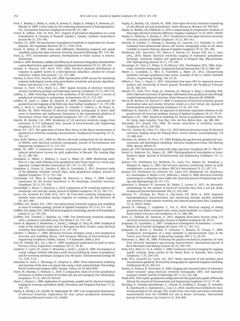
152 M.H. Loke et al. / Journal of Applied Geophysics 95 (2013) 135–156
Ferré, T., Bentley, L., Binley, A., Linde, N., Kemna, A., Singha, K., Holliger, K., Huisman, J.A.,Minsley, B., 2009. Critical steps for the continuing advancement of hydrogeophysics.Eos, Transactions American Geophysical Union 90 (23), 200.
Fortier, R., LeBlanc, A.M., Yu, W.B., 2011. Impacts of permafrost degradation on a roadembankment at Umiujaq in Nunavik (Quebec), Canada. Canadian GeotechnicalJournal 48 (5), 720–740.
Frasheri, A.I., 2009. The peculiarities of geophysical methods in exploration for chromedeposits. SEG Expanded Abstracts 28 (1), 1310–1314.
French, H., Binley, A., 2004. Snow melt infiltration: Monitoring temporal and spatialvariability using time-lapse electrical resistivity. Journal of Hydrology 297, 174–186.
Fried, J.J., 1975. Groundwater pollution. Developments in Water Science, 4. Elsevier,Amsterdam.
Friedel, S., 2003. Resolution, stability and efficiency of resistivity tomography estimated froma generalized inverse approach. Geophysical Journal International 153 (2), 305–316.
Furman, A., Warrick, A.W., Ferré, T.P.A., 2002. Electrical potential distributions inresponse to applied current in a heterogeneous subsurface, solution for circularinclusions. Vadose Zone Journal 1 (2), 273–280.
Furman, A., Ferré, T.P.A., Warrick, A.W., 2004. Optimization of ERT surveys for monitoringtransient hydrological events using perturbation sensitivity and genetic algorithms.Vadose Zone Journal 3 (4), 1230–1239.
Furman, A., Ferré, T.P.A., Heath, G.L., 2007. Spatial focusing of electrical resistivitysurveys considering geologic and hydrologic layering. Geophysics 72 (2), F65–F73.
Gaffney, C., 2008. Detecting trends in the prediction of the buried past: a review ofgeophysical techniques in archaeology. Archaeometry 50 (2), 313–336.
Gebbers, R., Lueck, E., Dabas, M., Domsch, H., 2009. Comparison of instruments forgeoelectrical soil mapping at the field scale. Near Surface Geophysics 7 (3), 179–190.
Gélis, C., Revil, A., Cushing, M.E., Jougnot, D., Lemeille, F., Cabrera, J., De Hoyos, A.,Rocher, M., 2010. Potential of electrical resistivity tomography to detect faultzones in limestone and argillaceous formations in the experimental platform ofTournemire, France. Pure and Applied Geophysics 167 (11), 1405–1418.
Gharibi, M., Bentley, L.R., 2005. Resolution of 3-D electrical resistivity images frominversions of 2-D orthogonal lines. Journal of Environmental and EngineeringGeophysics 10 (4), 339–349.
Ghosh, D.P., 1971. The application of linear filter theory to the direct interpretation ofgeoelectrical resistivity sounding measurements. Geophysical Prospecting 19 (2),192–217.
Goes, B.J.M., Meekes, J.A.C., 2004. An effective electrode configuration for the detectionof DNAPLs with electrical resistivity tomography. Journal of Environmental andEngineering Geophysics 9 (3), 127–141.
Goldie, M., 2007. A comparison between conventional and distributed acquisitioninduced polarization surveys for gold exploration in Nevada. The Leading Edge26 (2), 180–183.
Grandjean, G., Hibert, C., Mathieu, F., Garel, E., Malet, J.P., 2009. Monitoring waterflow in a clay–shale hillslope from geophysical data fusion based on a fuzzy logicapproach. Comptes Rendus Geosciences 341 (10–11), 937–948.
Grandjean, G., Gourry, J.C., Sanchez, O., Bitri, A., Garambois, S., 2011. Structural studyof the Ballandaz landslide (French Alps) using geophysical imagery. Journal ofApplied Geophysics 75 (3), 531–542.
Greenhalgh, S.A., Zhou, B., Greenhalgh, M., Marescot, L., Wiese, T., 2009. Explicitexpressions for the Frechet derivatives in 3D anisotropic resistivity inversion.Geophysics 70 (3), F31–F43.
Greenhalgh, S., Wiese, T., Marescot, L., 2010. Comparison of DC sensitivity patterns foranisotropic and isotropic media. Journal of Applied Geophysics 70 (2), 103–112.
Greve, A.K., Acworth, R.I., Kelly, B.F.J., 2011. 3D Cross-hole resistivity tomography tomonitor water percolation during irrigation on cracking soil. Soil Research 49(8), 661–669.
Griffiths, D.H., Barker, R.D., 1993. Two-dimensional resistivity imaging and modellingin areas of complex geology. Journal of Applied Geophysics 29 (3–4), 211–226.
Griffiths, D.H., Barker, R.D., 1994. Electrical imaging in archaeology. Journal of ArchaeologicalScience 21 (2), 153–158.
Griffiths, D.H., Turnbull, J., Olayinka, A.I., 1990. Two dimensional resistivity mappingwith a computer-controlled array. First Break 8 (4), 121–129.
Guerin, R., Begassat, P., Benderitter, Y., David, J., Tabbagh, A., Thiry, M., 2004. Geophysicalstudy of the industrial waste land in Mortagne-du-Nord (France) using electricalresistivity. Near Surface Geophysics 2 (3), 137–143.
Günther, T., Rücker, C., 2009. Advanced inversion strategies using a new geophysicalinversion and modelling library. 15th European Meeting of Environmental andEngineering Geophysics Dublin, Ireland, 7–9 September 2009, p. B14.
Guo, W., Dentith, M.C., Xu, J., Ren, F., 1999. Geophysical exploration for gold in GansuProvince, China. Exploration Geophysics 30 (2), 76–82.
Gutiérrez, F., Galve, J.P., Lucha, P., Bonachea, J., Jordá, L., Jordá, R., 2009. Investigation ofa large collapse sinkhole affecting a multi-storey building by means of geophysicsand the trenching technique (Zaragoza City, NE Spain). Environmental Geology 58(5), 1107–1122.
Hatanaka, H., Aono, T., Mizunaga, H., Ushijima, K., 2005. Three-dimensional modelingand inversion of the mise-a-la-masse data using a steel-casing borehole. ProceedingsWorld Geothermal Congress 2005. Antalya, Turkey, 24–29 April 2005.
Hatch, M., Munday, T., Heinson, G., 2010. A comparative study of in-river geophysicaltechniques to define variation of riverbed salt and aid managing river salinization.Geophysics 75 (4), WA135–WA147.
Hauck, C., Kneisel, C., 2006. Application of capacitively-coupled and DC electrical resistivityimaging for mountain permafrost studies. Permafrost and Periglacial Processes 17 (2),169–177.
Hayley, K., Bentley, L.R., Gharibi, M., Nightingale, M., 2007. Low temperature dependenceof electrical resistivity: implications for near surface geophysical monitoring.Geophysical Research Letters 34, L18402.
Hayley, K., Bentley, L.R., Gharibi, M., 2009. Time-lapse electrical resistivity monitoringof salt-affected soil and groundwater. Water Resources Research 45, W07425.
Hayley, K., Bentley, L.R., Pidlisecky, A., 2010. Compensating for temperature variations intime-lapse electrical resistivity difference imaging. Geophysics 75 (4), WA51–WA59.
Hayley, K., Pidisecky, A., Bentley, L., 2011. Simultaneous time-lapse electrical resistivityinversion. Journal of Applied Geophysics 75 (2), 401–411.
Heincke, B., Gunther, T., Dalsegg, E., Ronning, J.S., Ganerod, G.V., Elvebakk, H., 2010.Combined three-dimensional electric and seismic tomography study on the Aknesrockslide in western Norway. Journal of Applied Geophysics 70 (4), 292–306.
Henderson, R.D., Day-Lewis, F.D., Abarca, E., Harvey, C.F., Karam, H.N., Liu, L., Lane,J.W.J., 2010. Marine electrical resistivity imaging of submarine groundwaterdischarge: sensitivity analysis and application in Waquoit Bay, Massachusetts,USA. Hydrogeology Journal 18 (1), 173–185.
Herwanger, J.V., Pain, C.C., Binley, A., De Oliveira, C.R.E., Worthington, M.H., 2004. Aniso-tropic resistivity tomography. Geophysical Journal International 158 (2), 409–425.
Hibert, C., Grandjean, G., Bitri, A., Travelletti, J., Malet, J.P., 2012. Characterizinglandslides through geophysical data fusion: example of the La Valette landslide(France). Engineering Geology 128, 23–29.
Hilbich, C., Fuss, C., Hauck, C., 2011. Automated time-lapse ERT for improved processanalysis and monitoring of frozen ground. Permafrost and Periglacial Processes22 (4), 306–319.
Hinnell, A.C., Ferré, T.P.A., Vrugt, J.A., Huisman, J.A., Moysey, S., Rings, J., Kowalsky, M.B.,2010. Improved extraction of hydrologic information from geophysical data throughcoupled hydrogeophysical inversion. Water Resources Research 46, W00D40.
Hirsch, M., Bentley, L.R., Dietrich, P., 2008. A comparison of electrical resistivity, groundpenetrating radar and seismic refraction results at a river terrace site. Journal ofEnvironmental and Engineering Geophysics 13 (4), 325–333.
Hoffmann, R., Dietrich, P., 2004. An approach to determine equivalent solutions to thegeoelectrical 2D inversion problem. Journal of Applied Geophysics 56 (2), 79–91.
Hohmann, G.W., 1982. Numerical modeling for electrical geophysical methods. Proc.Int. Symp. Appl. Geophys. Trop. Reg., Univ. do Para, Belem, Braz. , pp. 308–384.
Holcombe, H.T., Jiracek, G.R., 1984. 3D terrain corrections in resistivity surveys.Geophysics 49 (4), 439–452.
Hsu, H.L., Yanites, B.J., Chen, C.C., Chen, Y.G., 2010. Bedrock detection using 2D electricalresistivity imaging along the Peikang River, central Taiwan. Geomorphology 114(3), 406–414.
Huisman, J.A., Bouten, W., Ferre, T.P., 2004. Bridging the gap between geophysical mea-surements and hydrological modelling. American Geophysical Union, Fall Meeting2004, abstract #H14C-01.
Inman, J.R., 1975. Resistivity inversion with ridge regression. Geophysics 40 (5), 798–817.Ismail, A., Anderson, N.L., Rogers, J.D., 2005. Hydrogeophysical investigation at Luxor,
Southern Egypt. Journal of Environmental and Engineering Geophysics 10 (1),35–50.
Jackson, P.D., Northmore, K.J., Meldrum, P.I., Gunn, D.A., Hallam, J.R., Wambura, J.,Wangusi, B., Ogutu, G., 2002. Non-invasive moisture monitoring within an earthembankment—a precursor to failure. NDT & E International 35 (2), 107–115.
Jackson, P.D., Northmore, K.J., Entwisle, D.C., Gunn, D.A., Milodowski, A.E., Boardman,D.I., Zourmpakis, A., Rogers, C.D.F., Jefferson, I., Dixon, N., 2006. Electrical resistivitymonitoring of a collapsing meta-stable soil. Quarterly Journal of Engineering Geol-ogy and Hydrogeology 39, 151–172.
Johansson, S., Rosqvist, H., Svensson, M., Dahlin, T., Leroux, V., 2011. An alternativemethodology for the analysis of electrical resistivity data from a soil gas study.Geophysical Journal International 186 (2), 632–640.
Johnson, T.C., Versteeg, R.J., Ward, A., Day-Lewis, F.D., Revil, A., 2010. Improvedhydrogeophysical characterization and monitoring through parallel modelingand inversion of time-domain resistivity and induced-polarization data. Geophysics75 (4), WA27–WA41.
Jomard, H., Lebourg, T., Guglielmi, Y., Tric, E., 2010. Electrical imaging of slidinggeometry and fluids associated with a deep seated landslide (La Clapiere, France).Earth Surface Processes and Landforms 35 (5), 588–599.
Jones, G., Zielinski, M., Sentenac, P., 2012. Mapping desiccation fissures using 3-Delectrical resistivity tomography. Journal of Applied Geophysics 84, 39–51.
Jongmans, D., Garambois, S., 2007. Geophysical investigation of landslides: a review.Bulletin de la Société Géologique de France 178 (2), 101–112.
Jongmans, D., Bievre, G., Renalier, F., Schwartz, S., Beaurez, N., Orengo, Y., 2009.Geophysical investigation of a large landslide in glaciolacustrine clays in theTrieves area (French Alps). Engineering Geology 109 (1–2), 45–56.
Kahraman, S., Alber, M., 2006. Predicting the physico-mechanical properties of rocksfrom electrical impedance spectroscopy measurements. International Journal ofRock Mechanics and Mining Sciences 43 (4), 543–553.
Kelly, B.F.J., Allen, D., Ye, K., Dahlin, T., 2009. Continuous electrical imaging for mappingaquifer recharge along reaches of the Namoi River in Australia. Near SurfaceGeophysics 7 (4), 259–270.
Kelly, B.F.J., Acworth, R.I., Greve, A.K., 2011. Better placement of soil moisture pointmeasurements guided by 2D resistivity tomography for improved irrigation scheduling.Soil Research 49 (6), 504–512.
Kemna, A., Kulessa, B., Vereecken, H., 2002. Imaging and characterisation of subsurfacesolute transport using electrical resistivity tomography (ERT) and equivalenttransport models. Journal of Hydrology 267 (3–4), 125–146.
Khalil,M.H., 2010. Hydro-geophysical configuration for the quaternary aquifer ofNuweibaAlluvial Fan. Journal of Environmental and Engineering Geophysics 15 (2), 77–90.
Kiessling, D., Schmidt-Hattenberger, C., Schuett, H., Schilling, F., Krueger, K., Schoebel,B., Danckwardt, E., Kummerow, J., Grp, C.S., 2010. Geoelectrical methods for mon-itoring geological CO2 storage: first results from cross-hole and surface-downholemeasurements from the CO2SINK test site at Ketzin (Germany). InternationalJournal of Greenhouse Gas Control 4 (5), 816–826.
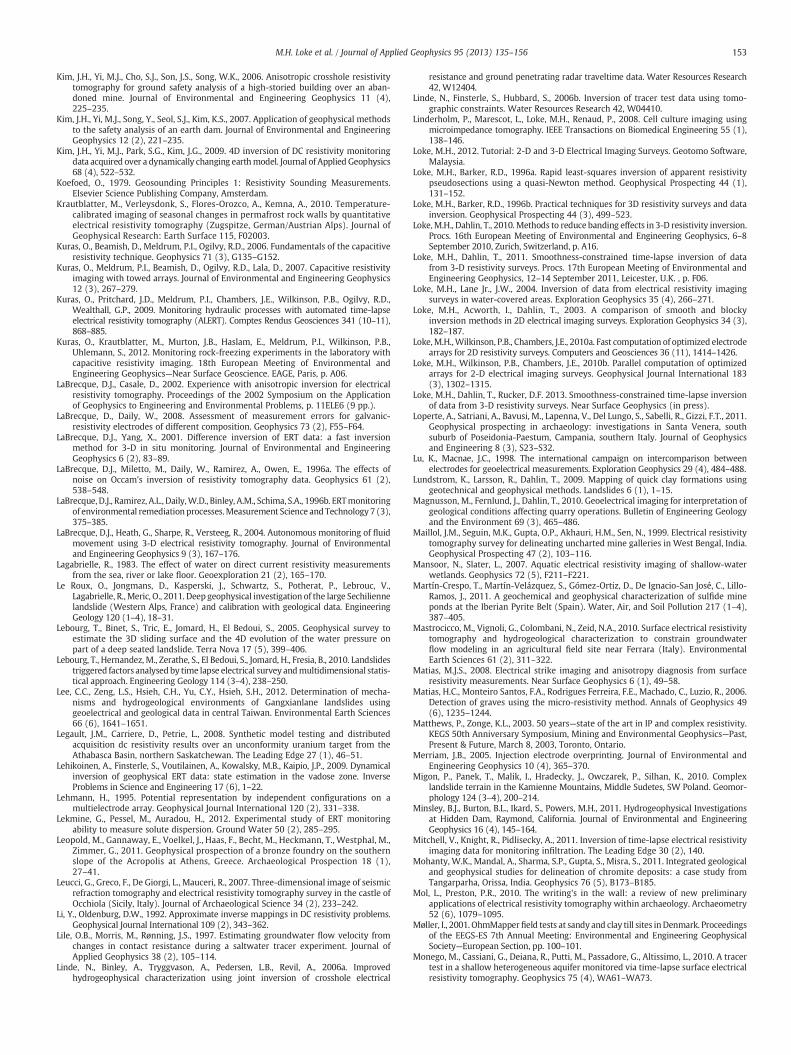
153M.H. Loke et al. / Journal of Applied Geophysics 95 (2013) 135–156
Kim, J.H., Yi, M.J., Cho, S.J., Son, J.S., Song, W.K., 2006. Anisotropic crosshole resistivitytomography for ground safety analysis of a high-storied building over an aban-doned mine. Journal of Environmental and Engineering Geophysics 11 (4),225–235.
Kim, J.H., Yi, M.J., Song, Y., Seol, S.J., Kim, K.S., 2007. Application of geophysical methodsto the safety analysis of an earth dam. Journal of Environmental and EngineeringGeophysics 12 (2), 221–235.
Kim, J.H., Yi, M.J., Park, S.G., Kim, J.G., 2009. 4D inversion of DC resistivity monitoringdata acquired over a dynamically changing earthmodel. Journal of Applied Geophysics68 (4), 522–532.
Koefoed, O., 1979. Geosounding Principles 1: Resistivity Sounding Measurements.Elsevier Science Publishing Company, Amsterdam.
Krautblatter, M., Verleysdonk, S., Flores-Orozco, A., Kemna, A., 2010. Temperature-calibrated imaging of seasonal changes in permafrost rock walls by quantitativeelectrical resistivity tomography (Zugspitze, German/Austrian Alps). Journal ofGeophysical Research: Earth Surface 115, F02003.
Kuras, O., Beamish, D., Meldrum, P.I., Ogilvy, R.D., 2006. Fundamentals of the capacitiveresistivity technique. Geophysics 71 (3), G135–G152.
Kuras, O., Meldrum, P.I., Beamish, D., Ogilvy, R.D., Lala, D., 2007. Capacitive resistivityimaging with towed arrays. Journal of Environmental and Engineering Geophysics12 (3), 267–279.
Kuras, O., Pritchard, J.D., Meldrum, P.I., Chambers, J.E., Wilkinson, P.B., Ogilvy, R.D.,Wealthall, G.P., 2009. Monitoring hydraulic processes with automated time-lapseelectrical resistivity tomography (ALERT). Comptes Rendus Geosciences 341 (10–11),868–885.
Kuras, O., Krautblatter, M., Murton, J.B., Haslam, E., Meldrum, P.I., Wilkinson, P.B.,Uhlemann, S., 2012. Monitoring rock-freezing experiments in the laboratory withcapacitive resistivity imaging. 18th European Meeting of Environmental andEngineering Geophysics—Near Surface Geoscience. EAGE, Paris, p. A06.
LaBrecque, D.J., Casale, D., 2002. Experience with anisotropic inversion for electricalresistivity tomography. Proceedings of the 2002 Symposium on the Applicationof Geophysics to Engineering and Environmental Problems, p. 11ELE6 (9 pp.).
LaBrecque, D., Daily, W., 2008. Assessment of measurement errors for galvanic-resistivity electrodes of different composition. Geophysics 73 (2), F55–F64.
LaBrecque, D.J., Yang, X., 2001. Difference inversion of ERT data: a fast inversionmethod for 3-D in situ monitoring. Journal of Environmental and EngineeringGeophysics 6 (2), 83–89.
LaBrecque, D.J., Miletto, M., Daily, W., Ramirez, A., Owen, E., 1996a. The effects ofnoise on Occam's inversion of resistivity tomography data. Geophysics 61 (2),538–548.
LaBrecque, D.J., Ramirez, A.L., Daily,W.D., Binley, A.M., Schima, S.A., 1996b. ERTmonitoringof environmental remediation processes.Measurement Science and Technology7 (3),375–385.
LaBrecque, D.J., Heath, G., Sharpe, R., Versteeg, R., 2004. Autonomous monitoring of fluidmovement using 3-D electrical resistivity tomography. Journal of Environmentaland Engineering Geophysics 9 (3), 167–176.
Lagabrielle, R., 1983. The effect of water on direct current resistivity measurementsfrom the sea, river or lake floor. Geoexploration 21 (2), 165–170.
Le Roux, O., Jongmans, D., Kasperski, J., Schwartz, S., Potherat, P., Lebrouc, V.,Lagabrielle, R.,Meric, O., 2011. Deep geophysical investigation of the large Sechiliennelandslide (Western Alps, France) and calibration with geological data. EngineeringGeology 120 (1–4), 18–31.
Lebourg, T., Binet, S., Tric, E., Jomard, H., El Bedoui, S., 2005. Geophysical survey toestimate the 3D sliding surface and the 4D evolution of the water pressure onpart of a deep seated landslide. Terra Nova 17 (5), 399–406.
Lebourg, T., Hernandez, M., Zerathe, S., El Bedoui, S., Jomard, H., Fresia, B., 2010. Landslidestriggered factors analysed by time lapse electrical survey andmultidimensional statis-tical approach. Engineering Geology 114 (3–4), 238–250.
Lee, C.C., Zeng, L.S., Hsieh, C.H., Yu, C.Y., Hsieh, S.H., 2012. Determination of mecha-nisms and hydrogeological environments of Gangxianlane landslides usinggeoelectrical and geological data in central Taiwan. Environmental Earth Sciences66 (6), 1641–1651.
Legault, J.M., Carriere, D., Petrie, L., 2008. Synthetic model testing and distributedacquisition dc resistivity results over an unconformity uranium target from theAthabasca Basin, northern Saskatchewan. The Leading Edge 27 (1), 46–51.
Lehikoinen, A., Finsterle, S., Voutilainen, A., Kowalsky, M.B., Kaipio, J.P., 2009. Dynamicalinversion of geophysical ERT data: state estimation in the vadose zone. InverseProblems in Science and Engineering 17 (6), 1–22.
Lehmann, H., 1995. Potential representation by independent configurations on amultielectrode array. Geophysical Journal International 120 (2), 331–338.
Lekmine, G., Pessel, M., Auradou, H., 2012. Experimental study of ERT monitoringability to measure solute dispersion. Ground Water 50 (2), 285–295.
Leopold, M., Gannaway, E., Voelkel, J., Haas, F., Becht, M., Heckmann, T., Westphal, M.,Zimmer, G., 2011. Geophysical prospection of a bronze foundry on the southernslope of the Acropolis at Athens, Greece. Archaeological Prospection 18 (1),27–41.
Leucci, G., Greco, F., De Giorgi, L., Mauceri, R., 2007. Three-dimensional image of seismicrefraction tomography and electrical resistivity tomography survey in the castle ofOcchiola (Sicily, Italy). Journal of Archaeological Science 34 (2), 233–242.
Li, Y., Oldenburg, D.W., 1992. Approximate inverse mappings in DC resistivity problems.Geophysical Journal International 109 (2), 343–362.
Lile, O.B., Morris, M., Rønning, J.S., 1997. Estimating groundwater flow velocity fromchanges in contact resistance during a saltwater tracer experiment. Journal ofApplied Geophysics 38 (2), 105–114.
Linde, N., Binley, A., Tryggvason, A., Pedersen, L.B., Revil, A., 2006a. Improvedhydrogeophysical characterization using joint inversion of crosshole electrical
resistance and ground penetrating radar traveltime data. Water Resources Research42, W12404.
Linde, N., Finsterle, S., Hubbard, S., 2006b. Inversion of tracer test data using tomo-graphic constraints. Water Resources Research 42, W04410.
Linderholm, P., Marescot, L., Loke, M.H., Renaud, P., 2008. Cell culture imaging usingmicroimpedance tomography. IEEE Transactions on Biomedical Engineering 55 (1),138–146.
Loke, M.H., 2012. Tutorial: 2-D and 3-D Electrical Imaging Surveys. Geotomo Software,Malaysia.
Loke, M.H., Barker, R.D., 1996a. Rapid least-squares inversion of apparent resistivitypseudosections using a quasi-Newton method. Geophysical Prospecting 44 (1),131–152.
Loke, M.H., Barker, R.D., 1996b. Practical techniques for 3D resistivity surveys and datainversion. Geophysical Prospecting 44 (3), 499–523.
Loke,M.H., Dahlin, T., 2010. Methods to reduce banding effects in 3-D resistivity inversion.Procs. 16th European Meeting of Environmental and Engineering Geophysics, 6–8September 2010, Zurich, Switzerland, p. A16.
Loke, M.H., Dahlin, T., 2011. Smoothness-constrained time-lapse inversion of datafrom 3-D resistivity surveys. Procs. 17th European Meeting of Environmental andEngineering Geophysics, 12–14 September 2011, Leicester, U.K. , p. F06.
Loke, M.H., Lane Jr., J.W., 2004. Inversion of data from electrical resistivity imagingsurveys in water-covered areas. Exploration Geophysics 35 (4), 266–271.
Loke, M.H., Acworth, I., Dahlin, T., 2003. A comparison of smooth and blockyinversion methods in 2D electrical imaging surveys. Exploration Geophysics 34 (3),182–187.
Loke,M.H.,Wilkinson, P.B., Chambers, J.E., 2010a. Fast computation of optimized electrodearrays for 2D resistivity surveys. Computers and Geosciences 36 (11), 1414–1426.
Loke, M.H., Wilkinson, P.B., Chambers, J.E., 2010b. Parallel computation of optimizedarrays for 2-D electrical imaging surveys. Geophysical Journal International 183(3), 1302–1315.
Loke, M.H., Dahlin, T., Rucker, D.F. 2013. Smoothness-constrained time-lapse inversionof data from 3-D resistivity surveys. Near Surface Geophysics (in press).
Loperte, A., Satriani, A., Bavusi, M., Lapenna, V., Del Lungo, S., Sabelli, R., Gizzi, F.T., 2011.Geophysical prospecting in archaeology: investigations in Santa Venera, southsuburb of Poseidonia-Paestum, Campania, southern Italy. Journal of Geophysicsand Engineering 8 (3), S23–S32.
Lu, K., Macnae, J.C., 1998. The international campaign on intercomparison betweenelectrodes for geoelectrical measurements. Exploration Geophysics 29 (4), 484–488.
Lundstrom, K., Larsson, R., Dahlin, T., 2009. Mapping of quick clay formations usinggeotechnical and geophysical methods. Landslides 6 (1), 1–15.
Magnusson, M., Fernlund, J., Dahlin, T., 2010. Geoelectrical imaging for interpretation ofgeological conditions affecting quarry operations. Bulletin of Engineering Geologyand the Environment 69 (3), 465–486.
Maillol, J.M., Seguin, M.K., Gupta, O.P., Akhauri, H.M., Sen, N., 1999. Electrical resistivitytomography survey for delineating uncharted mine galleries in West Bengal, India.Geophysical Prospecting 47 (2), 103–116.
Mansoor, N., Slater, L., 2007. Aquatic electrical resistivity imaging of shallow-waterwetlands. Geophysics 72 (5), F211–F221.
Martín-Crespo, T., Martín-Velázquez, S., Gómez-Ortiz, D., De Ignacio-San José, C., Lillo-Ramos, J., 2011. A geochemical and geophysical characterization of sulfide mineponds at the Iberian Pyrite Belt (Spain). Water, Air, and Soil Pollution 217 (1–4),387–405.
Mastrocicco, M., Vignoli, G., Colombani, N., Zeid, N.A., 2010. Surface electrical resistivitytomography and hydrogeological characterization to constrain groundwaterflow modeling in an agricultural field site near Ferrara (Italy). EnvironmentalEarth Sciences 61 (2), 311–322.
Matias, M.J.S., 2008. Electrical strike imaging and anisotropy diagnosis from surfaceresistivity measurements. Near Surface Geophysics 6 (1), 49–58.
Matias, H.C., Monteiro Santos, F.A., Rodrigues Ferreira, F.E., Machado, C., Luzio, R., 2006.Detection of graves using the micro-resistivity method. Annals of Geophysics 49(6), 1235–1244.
Matthews, P., Zonge, K.L., 2003. 50 years—state of the art in IP and complex resistivity.KEGS 50th Anniversary Symposium, Mining and Environmental Geophysics—Past,Present & Future, March 8, 2003, Toronto, Ontario.
Merriam, J.B., 2005. Injection electrode overprinting. Journal of Environmental andEngineering Geophysics 10 (4), 365–370.
Migon, P., Panek, T., Malik, I., Hradecky, J., Owczarek, P., Silhan, K., 2010. Complexlandslide terrain in the Kamienne Mountains, Middle Sudetes, SW Poland. Geomor-phology 124 (3–4), 200–214.
Minsley, B.J., Burton, B.L., Ikard, S., Powers, M.H., 2011. Hydrogeophysical Investigationsat Hidden Dam, Raymond, California. Journal of Environmental and EngineeringGeophysics 16 (4), 145–164.
Mitchell, V., Knight, R., Pidlisecky, A., 2011. Inversion of time-lapse electrical resistivityimaging data for monitoring infiltration. The Leading Edge 30 (2), 140.
Mohanty, W.K., Mandal, A., Sharma, S.P., Gupta, S., Misra, S., 2011. Integrated geologicaland geophysical studies for delineation of chromite deposits: a case study fromTangarparha, Orissa, India. Geophysics 76 (5), B173–B185.
Mol, L., Preston, P.R., 2010. The writing's in the wall: a review of new preliminaryapplications of electrical resistivity tomography within archaeology. Archaeometry52 (6), 1079–1095.
Møller, I., 2001. OhmMapperfield tests at sandy and clay till sites inDenmark. Proceedingsof the EEGS-ES 7th Annual Meeting: Environmental and Engineering GeophysicalSociety—European Section, pp. 100–101.
Monego, M., Cassiani, G., Deiana, R., Putti, M., Passadore, G., Altissimo, L., 2010. A tracertest in a shallow heterogeneous aquifer monitored via time-lapse surface electricalresistivity tomography. Geophysics 75 (4), WA61–WA73.
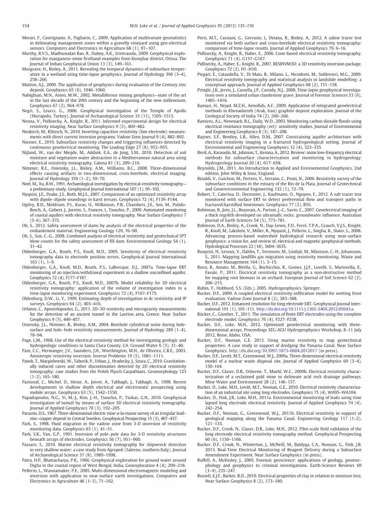
154 M.H. Loke et al. / Journal of Applied Geophysics 95 (2013) 135–156
Morari, F., Castrignano, A., Pagliarin, C., 2009. Application of multivariate geostatisticsin delineating management zones within a gravelly vineyard using geo-electricalsensors. Computers and Electronics in Agriculture 68 (1), 97–107.
Murthy, B.V.S., Madhusudan Rao, B., Dubey, A.K., Srinivasulu, 2009. Geophysical explo-ration for manganese-some firsthand examples from Keonjhar district, Orissa. TheJournal of Indian Geophysical Union 13 (3), 149–161.
Musgrave, H., Binley, A., 2011. Revealing the temporal dynamics of subsurface temper-ature in a wetland using time-lapse geophysics. Journal of Hydrology 396 (3–4),258–266.
Mutton, A.J., 2000. The application of geophysics during evaluation of the Century zincdeposit. Geophysics 65 (6), 1946–1960.
Nabighian, M.N., Asten, M.W., 2002. Metalliferous mining geophysics—state of the artin the last decade of the 20th century and the beginning of the new millennium.Geophysics 67 (3), 964–978.
Negri, S., Leucci, G., 2006. Geophysical investigation of the Temple of Apollo(Hierapolis, Turkey). Journal of Archaeological Science 33 (11), 1505–1513.
Nenna, V., Pidlisecky, A., Knight, R., 2011. Informed experimental design for electricalresistivity imaging. Near Surface Geophysics 9 (5), 469–482.
Neukirch, M., Klitzsch, N., 2010. Inverting capacitive resistivity (line electrode) measure-ments with direct current inversion programs. Vadose Zone Journal 9 (4), 882–892.
Niesner, E., 2010. Subsurface resistivity changes and triggering influences detected bycontinuous geoelectrical monitoring. The Leading Edge 27 (8), 952–955.
Nijland, W., van der Meijde, M., Addink, E.A., de Jong, S.M., 2010. Detection of soilmoisture and vegetation water abstraction in a Mediterranean natural area usingelectrical resistivity tomography. Catena 81 (3), 209–216.
Nimmer, R.E., Osiensky, J.L., Binley, A.M., Williams, B.C., 2008. Three-dimensionaleffects causing artifacts in two-dimensional, cross-borehole, electrical imaging.Journal of Hydrology 359 (1–2), 59–70.
Noel, M., Xu, B.W., 1991. Archaeological investigation by electrical-resistivity tomography—a preliminary-study. Geophysical Journal International 107 (1), 95–102.
Nyquist, J.E., Peake, J.S., Roth, M.J.S., 2007. Comparison of an optimized resistivity arraywith dipole–dipole soundings in karst terrain. Geophysics 72 (4), F139–F144.
Ogilvy, R.D., Meldrum, P.I., Kuras, O., Wilkinson, P.B., Chambers, J.E., Sen, M., Pulido-Bosch, A., Gisbert, J., Jorreto, S., Frances, I., Tsourlos, P., 2009. Automated monitoringof coastal aquifers with electrical resistivity tomography. Near Surface Geophysics 7(5–6), 367–375.
Oh, S., 2012. Safety assessment of dams by analysis of the electrical properties of theembankment material. Engineering Geology 129, 76–90.
Oh, S., Sun, C.-G., 2008. Combined analysis of electrical resistivity and geotechnical SPTblow counts for the safety assessment of fill dam. Environmental Geology 54 (1),31–42.
Oldenborger, G.A., Routh, P.S., Knoll, M.D., 2005. Sensitivity of electrical resistivitytomography data to electrode position errors. Geophysical Journal International163 (1), 1–9.
Oldenborger, G.A., Knoll, M.D., Routh, P.S., LaBrecque, D.J., 2007a. Time-lapse ERTmonitoring of an injection/withdrawal experiment in a shallow unconfined aquifer.Geophysics 72 (4), F177–F187.
Oldenborger, G.A., Routh, P.S., Knoll, M.D., 2007b. Model reliability for 3D electricalresistivity tomography: application of the volume of investigation index to atime-lapse monitoring experiment. Geophysics 72 (4), F167–F175.
Oldenburg, D.W., Li, Y., 1999. Estimating depth of investigation in dc resistivity and IPsurveys. Geophysics 64 (2), 403–416.
Orfanos, C., Apostolopoulos, G., 2011. 2D–3D resistivity and microgravity measurementsfor the detection of an ancient tunnel in the Lavrion area, Greece. Near SurfaceGeophysics 9 (5), 449–457.
Osiensky, J.L., Nimmer, R., Binley, A.M., 2004. Borehole cylindrical noise during hole-surface and hole–hole resistivity measurements. Journal of Hydrology 289 (1–4),78–94.
Page, L.M., 1968. Use of the electrical resistivity method for investigating geologic andhydrogeologic conditions in Santa Clara County, CA. Ground Water 6 (5), 31–40.
Pain, C.C., Herwanger, J.V., Saunders, J.H., Worthington, M.H., de Oliveira, C.R.E., 2003.Anisotropic resistivity inversion. Inverse Problems 19 (5), 1081–1111.
Panek, T., Margielewski,W., Taborik, P., Urban, J., Hradecky, J., Szura, C., 2010. Gravitation-ally induced caves and other discontinuities detected by 2D electrical resistivitytomography: case studies from the Polish Flysch Carpathians. Geomorphology 123(1–2), 165–180.
Panissod, C., Michel, D., Hesse, A., Joivet, A., Tabbagh, J., Tabbagh, A., 1998. Recentdevelopments in shallow depth electrical and electrostatic prospecting usingmobile arrays. Geophysics 63 (5), 1542–1550.
Papadopoulos, N.G., Yi, M.-J., Kim, J.-H., Tsourlos, P., Tsokas, G.N., 2010. Geophysicalinvestigation of tumuli by means of surface 3D electrical resistivity tomography.Journal of Applied Geophysics 70 (3), 192–205.
Parasnis, D.S., 1967. Three-dimensional electricmise-a-la-masse survey of an irregular lead–zinc–copper deposit in Central Sweden. Geophysical Prospecting 15 (3), 407–437.
Park, S., 1998. Fluid migration in the vadose zone from 3-D inversion of resistivitymonitoring data. Geophysics 63 (1), 41–51.
Park, S.K., Van, G.P., 1991. Inversion of pole–pole data for 3-D resistivity structuresbeneath arrays of electrodes. Geophysics 56 (7), 951–960.
Passaro, S., 2010. Marine electrical resistivity tomography for shipwreck detectionin very shallow water: a case study from Agropoli (Salerno, southern Italy). Journalof Archaeological Science 37 (8), 1989–1998.
Patra, H.P., Bhattacharya, P.K., 1966. Geophysical exploration for ground water aroundDigha in the coastal region of West Bengal, India. Geoexploration 4 (4), 209–218.
Pellerin, L., Wannamaker, P.E., 2005. Multi-dimensional electromagnetic modeling andinversion with application to near-surface earth investigations. Computers andElectronics in Agriculture 46 (1–3), 71–102.
Perri, M.T., Cassiani, G., Gervasio, I., Deiana, R., Binley, A., 2012. A saline tracer testmonitored via both surface and cross-borehole electrical resistivity tomography:comparison of time-lapse results. Journal of Applied Geophysics 79, 6–16.
Pidlisecky, A., Knight, R., Haber, E., 2006. Cone-based electrical resistivity tomography.Geophysics 71 (4), G157–G167.
Pidlisecky, A., Haber, E., Knight, R., 2007. RESINVM3D: a 3D resistivity inversion package.Geophysics 72 (2), H1–H10.
Piegari, E., Cataudella, V., Di Maio, R., Milano, L., Nicodemi, M., Soldovieri, M.G., 2009.Electrical resistivity tomography and statistical analysis in landslide modelling: aconceptual approach. Journal of Applied Geophysics 68 (2), 151–158.
Pringle, J.K., Jervis, J., Cassella, J.P., Cassidy, N.J., 2008. Time-lapse geophysical investiga-tions over a simulated urban clandestine grave. Journal of Forensic Sciences 53 (6),1405–1416.
Ramazi, H., Nejad, M.Z.H., Aenollah, A.F., 2009. Application of integrated geoelectricalmethods in Khenadarreh (Arak, Iran) graphite deposit exploration. Journal of theGeological Society of India 74 (2), 260–266.
Ramirez, A.L., Newmark, R.L., Daily, W.D., 2003. Monitoring carbon dioxide floods usingelectrical resistance tomography (ert): sensitivity studies. Journal of Environmentaland Engineering Geophysics 8 (3), 187–208.
Rayner, S.F., Bentley, L.R., Allen, D.M., 2007. Constraining aquifer architecture withelectrical resistivity imaging in a fractured hydrogeological setting. Journal ofEnvironmental and Engineering Geophysics 12 (4), 323–335.
Revil, A., Karaoulis, M., Johnson, T., Kemna, A., 2012. Review: some low-frequency electricalmethods for subsurface characterization and monitoring in hydrogeology.Hydrogeology Journal 20 (4), 617–658.
Reynolds, J.M., 2011. An Introduction to Applied and Environmental Geophysics, 2ndedition. John Wiley & Sons, England.
Rinaldi, V., Guichon, M., Ferrero, V., Serrano, C., Ponti, N., 2006. Resistivity survey of thesubsurface conditions in the estuary of the Rio de la Plata. Journal of Geotechnicaland Geoenvironmental Engineering 132 (1), 72–79.
Robert, T., Caterina, D., Deceuster, J., Kaufmann, O., Nguyen, F., 2012. A salt tracer testmonitored with surface ERT to detect preferential flow and transport paths infractured/karstified limestones. Geophysics 77 (2), B55.
Robineau, B., Join, J.L., Beauvais, A., Parisot, J.-C., Savin, C., 2007. Geoelectrical imaging ofa thick regolith developed on ultramafic rocks: groundwater influence. AustralianJournal of Earth Sciences 54 (5), 773–781.
Robinson, D.A., Binley, A., Crook, N., Day-Lewis, F.D., Ferré, T.P.A., Grauch, V.J.S., Knight,R., Knoll, M., Lakshmi, V., Miller, R., Nyquist, J., Pellerin, L., Singha, K., Slater, L., 2008.Advancing process-based watershed hydrological research using near-surfacegeophysics: a vision for, and review of, electrical and magnetic geophysical methods.Hydrological Processes 22 (18), 3604–3635.
Rosqvist, H., Leroux, V., Dahlin, T., Svensson, M., Lindsjö, M., Månsson, C.-H., Johansson,S., 2011. Mapping landfills gas migration using resistivity monitoring. Waste andResource Management 164 (1), 3–15.
Rossi, R., Amato, M., Bitella, G., Bochicchio, R., Gomes, J.J.F., Lovelli, S., Martorella, E.,Favale, P., 2011. Electrical resistivity tomography as a non-destructive methodfor mapping root biomass in an orchard. European Journal of Soil Science 62 (2),206–215.
Rubin, Y., Hubburd, S.S. (Eds.), 2005. Hydrogeophysics. Springer.Rucker, D.F., 2009. A coupled electrical resistivity-infiltration model for wetting front
evaluation. Vadose Zone Journal 8 (2), 383–388.Rucker, D.F., 2012. Enhanced resolution for long electrode ERT. Geophysical Journal Inter-
national 191 (1), 101–111. http://dx.doi.org/10.1111/j.1365-246X.2012.05643.x.Rücker, C., Günther, T., 2011. The simulation of finite ERT electrodes using the complete
electrode model. Geophysics 76 (4), F227–F238.Rucker, D.F., Loke, M.H., 2012. Optimized geoelectrical monitoring with three-
dimensional arrays. Proceedings SEG-AGU Hydrogeophysics Workshop, 8–11 July2012, Boise, Idaho, USA.
Rucker, D.F., Noonan, G.E. 2013. Using marine resistivity to map geotechnicalproperties: A case study in support of dredging the Panama Canal. Near SurfaceGeophysics. http://dx.doi.org/10.3997/1873-0604.2012017 (in press).
Rucker, D.F., Levitt, M.T., Greenwood, W.J., 2009a. Three-dimensional electrical resistivitymodel of a nuclear waste disposal site. Journal of Applied Geophysics 69 (3–4),150–164.
Rucker, D.F., Glaser, D.R., Osborne, T., Maehl, W.C., 2009b. Electrical resistivity charac-terization of a reclaimed gold mine to delineate acid rock drainage pathways.Mine Water and Environment 28 (2), 146–157.
Rucker, D., Loke, M.H., Levitt, M.T., Noonan, G.E., 2010. Electrical resistivity characteriza-tion of an industrial site using long electrodes. Geophysics 75 (4), WA95–WA104.
Rucker, D., Fink, J.B., Loke, M.H., 2011a. Environmental monitoring of leaks using timelapsed long electrode electrical resistivity. Journal of Applied Geophysics 74 (4),242–254.
Rucker, D.F., Noonan, G., Greenwood, W.J., 2011b. Electrical resistivity in support ofgeological mapping along the Panama Canal. Engineering Geology 117 (1–2),121–133.
Rucker, D.F., Crook, N., Glaser, D.R., Loke, M.H., 2012. Pilot-scale field validation of thelong electrode electrical resistivity tomography method. Geophysical Prospecting60 (6), 1150–1166.
Rucker, D.F., Crook, N., Winterton, J., McNeill, M., Baldyga, C.A., Noonan, G., Fink, J.B.2013. Real-Time Electrical Monitoring of Reagent Delivery during a SubsurfaceAmendment Experiment. Near Surface Geophysics (in press).
Ruffell, A., McKinley, J., 2005. Forensic geoscience: applications of geology, geomor-phology and geophysics to criminal investigations. Earth-Science Reviews 69(3–4), 235–247.
Russell, E.J.F., Barker, R.D., 2010. Electrical properties of clay in relation to moisture loss.Near Surface Geophysics 8 (2), 173–180.
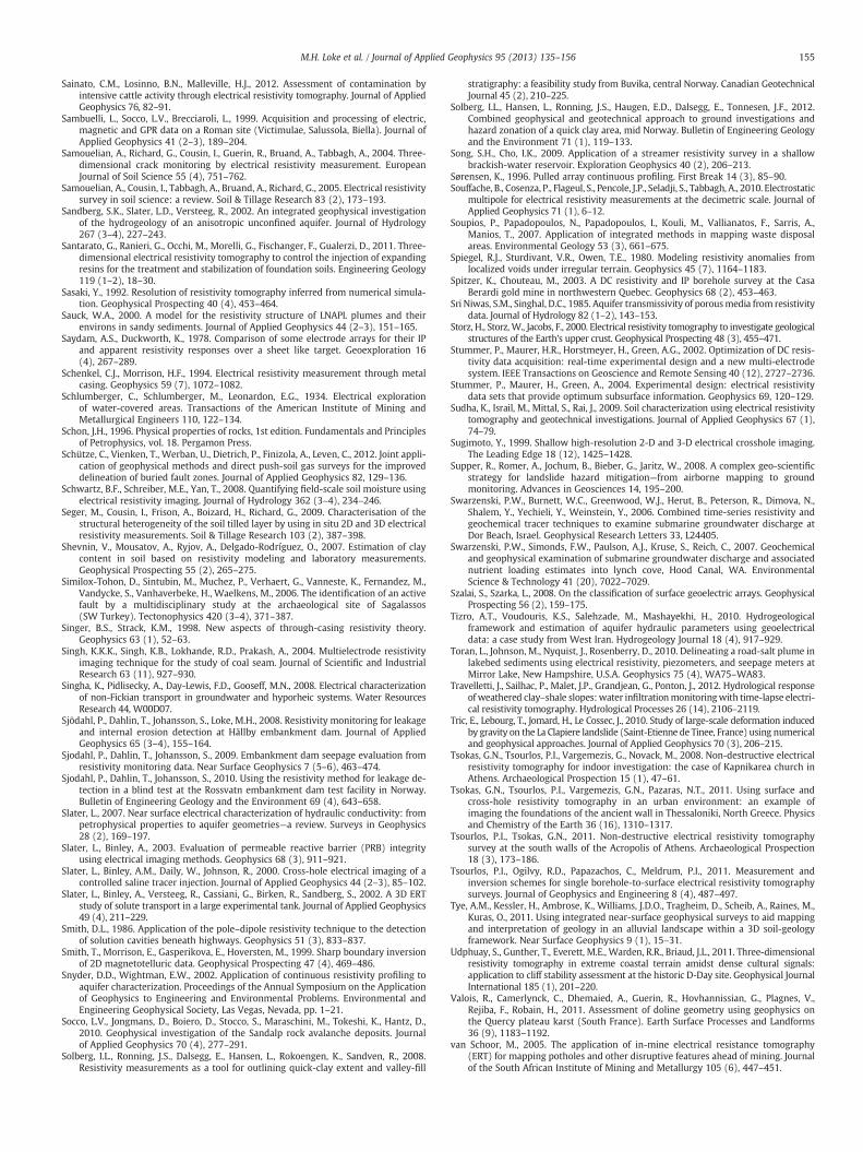
155M.H. Loke et al. / Journal of Applied Geophysics 95 (2013) 135–156
Sainato, C.M., Losinno, B.N., Malleville, H.J., 2012. Assessment of contamination byintensive cattle activity through electrical resistivity tomography. Journal of AppliedGeophysics 76, 82–91.
Sambuelli, L., Socco, L.V., Brecciaroli, L., 1999. Acquisition and processing of electric,magnetic and GPR data on a Roman site (Victimulae, Salussola, Biella). Journal ofApplied Geophysics 41 (2–3), 189–204.
Samouelian, A., Richard, G., Cousin, I., Guerin, R., Bruand, A., Tabbagh, A., 2004. Three-dimensional crack monitoring by electrical resistivity measurement. EuropeanJournal of Soil Science 55 (4), 751–762.
Samouelian, A., Cousin, I., Tabbagh, A., Bruand, A., Richard, G., 2005. Electrical resistivitysurvey in soil science: a review. Soil & Tillage Research 83 (2), 173–193.
Sandberg, S.K., Slater, L.D., Versteeg, R., 2002. An integrated geophysical investigationof the hydrogeology of an anisotropic unconfined aquifer. Journal of Hydrology267 (3–4), 227–243.
Santarato, G., Ranieri, G., Occhi, M., Morelli, G., Fischanger, F., Gualerzi, D., 2011. Three-dimensional electrical resistivity tomography to control the injection of expandingresins for the treatment and stabilization of foundation soils. Engineering Geology119 (1–2), 18–30.
Sasaki, Y., 1992. Resolution of resistivity tomography inferred from numerical simula-tion. Geophysical Prospecting 40 (4), 453–464.
Sauck, W.A., 2000. A model for the resistivity structure of LNAPL plumes and theirenvirons in sandy sediments. Journal of Applied Geophysics 44 (2–3), 151–165.
Saydam, A.S., Duckworth, K., 1978. Comparison of some electrode arrays for their IPand apparent resistivity responses over a sheet like target. Geoexploration 16(4), 267–289.
Schenkel, C.J., Morrison, H.F., 1994. Electrical resistivity measurement through metalcasing. Geophysics 59 (7), 1072–1082.
Schlumberger, C., Schlumberger, M., Leonardon, E.G., 1934. Electrical explorationof water-covered areas. Transactions of the American Institute of Mining andMetallurgical Engineers 110, 122–134.
Schon, J.H., 1996. Physical properties of rocks, 1st edition. Fundamentals and Principlesof Petrophysics, vol. 18. Pergamon Press.
Schütze, C., Vienken, T., Werban, U., Dietrich, P., Finizola, A., Leven, C., 2012. Joint appli-cation of geophysical methods and direct push-soil gas surveys for the improveddelineation of buried fault zones. Journal of Applied Geophysics 82, 129–136.
Schwartz, B.F., Schreiber, M.E., Yan, T., 2008. Quantifying field-scale soil moisture usingelectrical resistivity imaging. Journal of Hydrology 362 (3–4), 234–246.
Seger, M., Cousin, I., Frison, A., Boizard, H., Richard, G., 2009. Characterisation of thestructural heterogeneity of the soil tilled layer by using in situ 2D and 3D electricalresistivity measurements. Soil & Tillage Research 103 (2), 387–398.
Shevnin, V., Mousatov, A., Ryjov, A., Delgado-Rodríguez, O., 2007. Estimation of claycontent in soil based on resistivity modeling and laboratory measurements.Geophysical Prospecting 55 (2), 265–275.
Similox-Tohon, D., Sintubin, M., Muchez, P., Verhaert, G., Vanneste, K., Fernandez, M.,Vandycke, S., Vanhaverbeke, H., Waelkens, M., 2006. The identification of an activefault by a multidisciplinary study at the archaeological site of Sagalassos(SW Turkey). Tectonophysics 420 (3–4), 371–387.
Singer, B.S., Strack, K.M., 1998. New aspects of through-casing resistivity theory.Geophysics 63 (1), 52–63.
Singh, K.K.K., Singh, K.B., Lokhande, R.D., Prakash, A., 2004. Multielectrode resistivityimaging technique for the study of coal seam. Journal of Scientific and IndustrialResearch 63 (11), 927–930.
Singha, K., Pidlisecky, A., Day-Lewis, F.D., Gooseff, M.N., 2008. Electrical characterizationof non-Fickian transport in groundwater and hyporheic systems. Water ResourcesResearch 44, W00D07.
Sjödahl, P., Dahlin, T., Johansson, S., Loke, M.H., 2008. Resistivity monitoring for leakageand internal erosion detection at Hällby embankment dam. Journal of AppliedGeophysics 65 (3–4), 155–164.
Sjodahl, P., Dahlin, T., Johansson, S., 2009. Embankment dam seepage evaluation fromresistivity monitoring data. Near Surface Geophysics 7 (5–6), 463–474.
Sjodahl, P., Dahlin, T., Johansson, S., 2010. Using the resistivity method for leakage de-tection in a blind test at the Rossvatn embankment dam test facility in Norway.Bulletin of Engineering Geology and the Environment 69 (4), 643–658.
Slater, L., 2007. Near surface electrical characterization of hydraulic conductivity: frompetrophysical properties to aquifer geometries—a review. Surveys in Geophysics28 (2), 169–197.
Slater, L., Binley, A., 2003. Evaluation of permeable reactive barrier (PRB) integrityusing electrical imaging methods. Geophysics 68 (3), 911–921.
Slater, L., Binley, A.M., Daily, W., Johnson, R., 2000. Cross-hole electrical imaging of acontrolled saline tracer injection. Journal of Applied Geophysics 44 (2–3), 85–102.
Slater, L., Binley, A., Versteeg, R., Cassiani, G., Birken, R., Sandberg, S., 2002. A 3D ERTstudy of solute transport in a large experimental tank. Journal of Applied Geophysics49 (4), 211–229.
Smith, D.L., 1986. Application of the pole–dipole resistivity technique to the detectionof solution cavities beneath highways. Geophysics 51 (3), 833–837.
Smith, T., Morrison, E., Gasperikova, E., Hoversten, M., 1999. Sharp boundary inversionof 2D magnetotelluric data. Geophysical Prospecting 47 (4), 469–486.
Snyder, D.D., Wightman, E.W., 2002. Application of continuous resistivity profiling toaquifer characterization. Proceedings of the Annual Symposium on the Applicationof Geophysics to Engineering and Environmental Problems. Environmental andEngineering Geophysical Society, Las Vegas, Nevada, pp. 1–21.
Socco, L.V., Jongmans, D., Boiero, D., Stocco, S., Maraschini, M., Tokeshi, K., Hantz, D.,2010. Geophysical investigation of the Sandalp rock avalanche deposits. Journalof Applied Geophysics 70 (4), 277–291.
Solberg, I.L., Ronning, J.S., Dalsegg, E., Hansen, L., Rokoengen, K., Sandven, R., 2008.Resistivity measurements as a tool for outlining quick-clay extent and valley-fill
stratigraphy: a feasibility study from Buvika, central Norway. Canadian GeotechnicalJournal 45 (2), 210–225.
Solberg, I.L., Hansen, L., Ronning, J.S., Haugen, E.D., Dalsegg, E., Tonnesen, J.F., 2012.Combined geophysical and geotechnical approach to ground investigations andhazard zonation of a quick clay area, mid Norway. Bulletin of Engineering Geologyand the Environment 71 (1), 119–133.
Song, S.H., Cho, I.K., 2009. Application of a streamer resistivity survey in a shallowbrackish-water reservoir. Exploration Geophysics 40 (2), 206–213.
Sørensen, K., 1996. Pulled array continuous profiling. First Break 14 (3), 85–90.Souffache, B., Cosenza, P., Flageul, S., Pencole, J.P., Seladji, S., Tabbagh, A., 2010. Electrostatic
multipole for electrical resistivity measurements at the decimetric scale. Journal ofApplied Geophysics 71 (1), 6–12.
Soupios, P., Papadopoulos, N., Papadopoulos, I., Kouli, M., Vallianatos, F., Sarris, A.,Manios, T., 2007. Application of integrated methods in mapping waste disposalareas. Environmental Geology 53 (3), 661–675.
Spiegel, R.J., Sturdivant, V.R., Owen, T.E., 1980. Modeling resistivity anomalies fromlocalized voids under irregular terrain. Geophysics 45 (7), 1164–1183.
Spitzer, K., Chouteau, M., 2003. A DC resistivity and IP borehole survey at the CasaBerardi gold mine in northwestern Quebec. Geophysics 68 (2), 453–463.
Sri Niwas, S.M., Singhal, D.C., 1985. Aquifer transmissivity of porousmedia from resistivitydata. Journal of Hydrology 82 (1–2), 143–153.
Storz, H., Storz, W., Jacobs, F., 2000. Electrical resistivity tomography to investigate geologicalstructures of the Earth's upper crust. Geophysical Prospecting 48 (3), 455–471.
Stummer, P., Maurer, H.R., Horstmeyer, H., Green, A.G., 2002. Optimization of DC resis-tivity data acquisition: real-time experimental design and a new multi-electrodesystem. IEEE Transactions on Geoscience and Remote Sensing 40 (12), 2727–2736.
Stummer, P., Maurer, H., Green, A., 2004. Experimental design: electrical resistivitydata sets that provide optimum subsurface information. Geophysics 69, 120–129.
Sudha, K., Israil, M., Mittal, S., Rai, J., 2009. Soil characterization using electrical resistivitytomography and geotechnical investigations. Journal of Applied Geophysics 67 (1),74–79.
Sugimoto, Y., 1999. Shallow high-resolution 2-D and 3-D electrical crosshole imaging.The Leading Edge 18 (12), 1425–1428.
Supper, R., Romer, A., Jochum, B., Bieber, G., Jaritz, W., 2008. A complex geo-scientificstrategy for landslide hazard mitigation—from airborne mapping to groundmonitoring. Advances in Geosciences 14, 195–200.
Swarzenski, P.W., Burnett, W.C., Greenwood, W.J., Herut, B., Peterson, R., Dimova, N.,Shalem, Y., Yechieli, Y., Weinstein, Y., 2006. Combined time-series resistivity andgeochemical tracer techniques to examine submarine groundwater discharge atDor Beach, Israel. Geophysical Research Letters 33, L24405.
Swarzenski, P.W., Simonds, F.W., Paulson, A.J., Kruse, S., Reich, C., 2007. Geochemicaland geophysical examination of submarine groundwater discharge and associatednutrient loading estimates into lynch cove, Hood Canal, WA. EnvironmentalScience & Technology 41 (20), 7022–7029.
Szalai, S., Szarka, L., 2008. On the classification of surface geoelectric arrays. GeophysicalProspecting 56 (2), 159–175.
Tizro, A.T., Voudouris, K.S., Salehzade, M., Mashayekhi, H., 2010. Hydrogeologicalframework and estimation of aquifer hydraulic parameters using geoelectricaldata: a case study from West Iran. Hydrogeology Journal 18 (4), 917–929.
Toran, L., Johnson, M., Nyquist, J., Rosenberry, D., 2010. Delineating a road-salt plume inlakebed sediments using electrical resistivity, piezometers, and seepage meters atMirror Lake, New Hampshire, U.S.A. Geophysics 75 (4), WA75–WA83.
Travelletti, J., Sailhac, P., Malet, J.P., Grandjean, G., Ponton, J., 2012. Hydrological responseof weathered clay–shale slopes:water infiltrationmonitoringwith time-lapse electri-cal resistivity tomography. Hydrological Processes 26 (14), 2106–2119.
Tric, E., Lebourg, T., Jomard, H., Le Cossec, J., 2010. Study of large-scale deformation inducedby gravity on the La Clapiere landslide (Saint-Etienne de Tinee, France) using numericaland geophysical approaches. Journal of Applied Geophysics 70 (3), 206–215.
Tsokas, G.N., Tsourlos, P.I., Vargemezis, G., Novack, M., 2008. Non-destructive electricalresistivity tomography for indoor investigation: the case of Kapnikarea church inAthens. Archaeological Prospection 15 (1), 47–61.
Tsokas, G.N., Tsourlos, P.I., Vargemezis, G.N., Pazaras, N.T., 2011. Using surface andcross-hole resistivity tomography in an urban environment: an example ofimaging the foundations of the ancient wall in Thessaloniki, North Greece. Physicsand Chemistry of the Earth 36 (16), 1310–1317.
Tsourlos, P.I., Tsokas, G.N., 2011. Non-destructive electrical resistivity tomographysurvey at the south walls of the Acropolis of Athens. Archaeological Prospection18 (3), 173–186.
Tsourlos, P.I., Ogilvy, R.D., Papazachos, C., Meldrum, P.I., 2011. Measurement andinversion schemes for single borehole-to-surface electrical resistivity tomographysurveys. Journal of Geophysics and Engineering 8 (4), 487–497.
Tye, A.M., Kessler, H., Ambrose, K., Williams, J.D.O., Tragheim, D., Scheib, A., Raines, M.,Kuras, O., 2011. Using integrated near-surface geophysical surveys to aid mappingand interpretation of geology in an alluvial landscape within a 3D soil-geologyframework. Near Surface Geophysics 9 (1), 15–31.
Udphuay, S., Gunther, T., Everett, M.E., Warden, R.R., Briaud, J.L., 2011. Three-dimensionalresistivity tomography in extreme coastal terrain amidst dense cultural signals:application to cliff stability assessment at the historic D-Day site. Geophysical JournalInternational 185 (1), 201–220.
Valois, R., Camerlynck, C., Dhemaied, A., Guerin, R., Hovhannissian, G., Plagnes, V.,Rejiba, F., Robain, H., 2011. Assessment of doline geometry using geophysics onthe Quercy plateau karst (South France). Earth Surface Processes and Landforms36 (9), 1183–1192.
van Schoor, M., 2005. The application of in-mine electrical resistance tomography(ERT) for mapping potholes and other disruptive features ahead of mining. Journalof the South African Institute of Mining and Metallurgy 105 (6), 447–451.
156 M.H. Loke et al. / Journal of Applied Geophysics 95 (2013) 135–156
van Schoor,M., Binley, A., 2010. In-mine (tunnel-to-tunnel) electrical resistance tomographyin South African platinummines. Near Surface Geophysics 8 (6), 563–574.
Veeken, P.C.H., Legeydo, P.J., Davidenko, Y.A., Kudryavceva, E.O., Ivanov, S.A., Chuvaev, A.,2009. Benefits of the induced polarization geoelectric method to hydrocarbon explo-ration. Geophysics 74 (2), B47–B59.
Wait, J.R., 1982. Geo-Electromagnetism. Academic Press, New York.Wake, T.A., Mojica, A.O., Davis, M.H., Campbell, C.J., Mendizabal, T., 2012. Electrical
resistivity surveying and pseudo-three-dimensional tomographic imaging at SitioDrago, Bocas del Toro, Panama. Archaeological Prospection 19 (1), 49–58.
Ward, S.H., 1990. Resistivity and induced polarization methods. In: Ward, S.H. (Ed.),Geotechnical and Environmental Geophysics. Investigations in Geophysics No. 5.SEG, USA, pp. 147–190.
Ward, S.H., Hohmann, G.W., 1987. Electromagnetic theory for geophysical applications.In: Nabighian, M.N. (Ed.), Electromagnetic Methods in Applied Geophysics,Volume 1, Theory. Investigations in Geophysics No. 3. SEG.
West, L.J., Stewart, D.I., Binley, A.M., Shaw, B., 1999. Resistivity imaging of soil duringelectrokinetic transport. Engineering Geology 53 (2), 205–215.
White, P.A., 1988. Measurement of ground-water parameters using salt-water injectionand surface resistivity. GroundWater 26 (2), 179–186.
White, R.M.S., Collins, S., Denne, R., Hee, R., Brown, P., 2001. A new survey design for 3DIP modelling at Copper hill. Exploration Geophysics 32 (4), 152–155.
Wilkinson, P.B., Chambers, J.E., Meldrum, P.I., Ogilvy, R.D., Mellor, C.J., Caunt, S., 2005.A comparison of self-potential tomography with electrical resistivity tomogra-phy for the detection of abandoned mineshafts. Journal of Environmental andEngineering Geophysics 10 (4), 381–389.
Wilkinson, P.B., Chambers, J.E., Meldrum, P.I., Ogilvy, R.D., Caunt, S., 2006a. Optimiza-tion of array configurations and panel combinations for the detection and imagingof abandoned mineshafts using 3D cross-hole electrical resistivity tomography.Journal of Environmental and Engineering Geophysics 11 (3), 213–221.
Wilkinson, P.B., Meldrum, P.I., Chambers, J.E., Kuras, O., Ogilvy, R.D., 2006b. Improvedstrategies for the automatic selection of optimized sets of electrical resistivitytomography measurement configurations. Geophysical Journal International 167(3), 1119–1126.
Wilkinson, P.B., Chambers, J.E., Lelliott, M., Wealthall, G.P., Ogilvy, R.D., 2008. Extremesensitivity of crosshole electrical resistivity tomography measurements to geometricerrors. Geophysical Journal International 173 (1), 49–62.
Wilkinson, P.B., Chambers, J.E., Meldrum, P.I., Gunn, D.A., Ogilvy, R.D., Kuras, O., 2010a.Predicting the movements of permanently installed electrodes on an activelandslide using time-lapse geoelectrical resistivity data only. Geophysical JournalInternational 183 (2), 543–556.
Wilkinson, P.B., Meldrum, P.I., Kuras, O., Cambers, J.E., Holyoake, S.J., Ogilvy, R.D.,2010b. High-resolution electrical resistivity tomography monitoring of a tracertest in a confined aquifer. Journal of Applied Geophysics 70 (4), 268–276.
Wilkinson, P.B., Loke, M.H., Meldrum, P.I., Chambers, J.E., Kuras, O., Gunn, D.A., Ogilvy,R.D., 2012a. Practical aspects of applied optimized survey design for electricalresistivity tomography. Geophysical Journal International 189 (1), 428–440.
Wilkinson, P.B., Chambers, J.E., Meldrum, P.I., Kuras, O., Munro, C.J., 2012b. The robustnessand general applicability of optimal resistivity surveys designed bymaximisingmodelresolution. Proceedings 18th EuropeanMeeting of EAGENear Surface Geoscience, 3–5September 2012, Paris, France, p. B33.
Wilson, S.R., Ingham, M., McConchie, J.A., 2006. The applicability of earth resistivitymethods for saline interface definition. Journal of Hydrology 316 (1–4), 301–312.
Wisen, R., Auken, E., Dahlin, T., 2005. Combination of ID laterally constrained inversionand smooth inversion of resistivity data with a priori data from boreholes. NearSurface Geophysics 3 (2), 71–78.
Wiwattanachang, N., Giao, P.H., 2011. Monitoring crack development in fiber concrete beamby using electrical resistivity imaging. Journal of Applied Geophysics 75 (2), 294–304.
Xu, S.Z., 2001. The boundary element method in geophysics. Geophysical MonographSeries Number 9SEG, USA.
Yamakawa, Y., Kosugi, K., Masaoka, N., Tada, Y., Mizuyama, T., 2010. Use of a combinedpenetrometer-moisture probe together with geophysical methods to surveyhydrological properties of a natural slope. Vadose Zone Journal 9 (3), 768–779.
Yi, M.-Y., Kim, J.-H., Son, J.-S., 2009. Borehole deviation effect in electrical resistivitytomography. Geosciences Journal 13 (1), 87–102.
Zerathe, S., Lebourg, T., 2012. Evolution stages of large deep-seated landslides at thefront of a subalpine meridional chain (Maritime-Alps, France). Geomorphology138 (1), 390–403.
Zhe, J., Greenhalgh, S., Marescot, L., 2007. Multichannel, full waveform and flexibleelectrode combination resistivity-imaging system. Geophysics 72 (2), F57–F64.
Zhou, B., Dahlin, T., 2003. Properties and effects of measurement errors on 2D resistivityimaging surveying. Near Surface Geophysics 1 (3), 105–117.
Zhou, B., Greenhalgh, S.A., 2000. Cross-hole resistivity tomography using differentelectrode configurations. Geophysical Prospecting 48 (5), 887–912.
Zhou,W., Beck, B.F., Stephenson, J.B., 2000. Reliability of dipole–dipole electrical resistivitytomography for defining depth to bedrock in covered karst terranes. EnvironmentalGeology 39 (3), 760–766.
Zhou, W., Beck, B.F., Adams, A.L., 2002. Effective electrode array in mapping karst hazardsin electrical resistivity tomography. Environmental Geology 42 (8), 922–928.
Zhu, T., Feng, R., 2011. Resistivity tomography with a vertical line source and its appli-cation to the evaluation of residual oil saturation. Journal of Applied Geophysics 73(2), 155–163.
Zhu, J., Currens, J.C., Dinger, J.S., 2012. Challenges of using electrical resistivity methodto locate karst conduits—a field case in the Inner Bluegrass Region, Kentucky.Journal of Applied Geophysics 75 (3), 523–530.
Zohdy, A.A.R., Jackson, D.B., 1969. Application of deep electrical soundings for ground-water exploration in Hawaii. Geophysics 34 (4), 584–600.