Recent developments and applications in geotechnical field

investigations for deep foundations

Mayne, P.W.(1) and Niazi, F.S.(2)

(1) Georgia Institute of Technology, Atlanta, Georgia, USA <paul.mayne@ce.gatech.edu> (2) Indiana University - Purdue University, Fort Wayne, Indiana, USA <niazif@ipfw.edu>

ABSTRACT. For routine site investigations, the use of hybrid tools such as the seismic piezocone

and seismic flat dilatometer offer superior efficiency and economy to provide sufficient profiling

of subsurface conditions and the evaluation of geoparameters, as compared with routine soil

boring, drilling, and sampling. A single sounding provides up to five separate measurements on

soil behavior that can be used to calculate capacity and displacements for axial and lateral pile

foundation capacity, as well as in applications involving quality control for ground modification

projects. Axial pile capacity can be assessed using traditional approaches that utilize limit plasticity

and static equilibrium, or alternatively via direct in-situ testing methods. Load tests from a bridge

project in Minnesota are presented to illustrate the applicability of seismic piezocone testing.

1. INTRODUCTION

Each and every civil & environmental project requires a geotechnical site investigation to

determine the makeup of the underlying ground at that particular location. This can be

accomplished today using a combination and assortment of geophysical methods, soil drilling &

sampling for laboratory testing, and in-situ field testing.

There are currently many different types of deep foundation systems being used commercially

in support of civil engineering works for building loads, bridge piers, ports, and tower structures

both onshore and offshore. Pile types can include driven steel H and pipe (open-end versus closed-

end), precast versus prestressed concrete, timber, composite, tapered, and monotubes, or systems

of bored or augered deep foundations, such as cased or uncased drilled piers, slurry shafts,

augercast pilings, and caissons, as well as specialty types (e.g., Fundex, Omega, Screw, Dewaal).

Consequently, the notion that a single test number such as the SPT-N value can suffice for all the

needs in the analysis and design of modern piling foundations must be replaced with a more

rational belief that multiple measurements are paramount.

Herein, we shall explore the utilization of more modern tests, such as the seismic cone and

seismic dilatometer, for the collection of several measurements concerning soil behavior. In

addition to assessing soil stratigraphy and geoparameters in an efficient and economic manner,

these tests permit an evaluation of the nonlinear axial load-displacement response of deep

foundations.

1.1 Conventional Site Investigation

For the past century, the conventional approach to geotechnical subsurface investigation has been

the use of rotary drilling, augering, and sampling methods to create boreholes. Most common, the

use of open drive samplers permits the collection of small disturbed cylindrical soil specimens via

the standard penetration test (SPT). This provides a crude index (N-value) that needs an important

Page 2

correction for the energy inefficiency of various drop hammer systems in use since its debut in

1902, including: pinweight, donut, safety, and automatic hammers.

At the time that the geotechnical profession became aware of the energy efficiency issues

(Seed et al. 1985; Skempton 1986), the average energy efficiency of SPTs in practice was

approximately 60%, so this became the reference value for the correction, designated; N60, which

is obtained:

N60 = CE ∙ Nmeasured = (ER/60) ∙ Nmeasured

where CE = correction factor for energy efficiency

ER = energy ratio for the particular hammer system used (ASTM D 4633)

Nmeasured = number of hammer blows to drive a split-spoon sampler a vertical distance of

300 mm (or 1 foot), reported as blows/0.3 m.

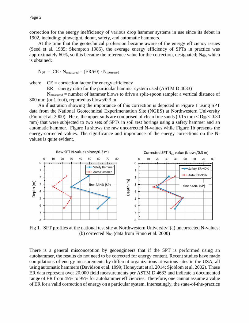
An illustration showing the importance of this correction is depicted in Figure 1 using SPT

data from the National Geotechnical Experimentation Site (NGES) at Northwestern University

(Finno et al. 2000). Here, the upper soils are comprised of clean fine sands (0.15 mm < D50 < 0.30

mm) that were subjected to two sets of SPTs in soil test borings using a safety hammer and an

automatic hammer. Figure 1a shows the raw uncorrected N-values while Figure 1b presents the

energy-corrected values. The significance and importance of the energy corrections on the N-

values is quite evident.

Fig 1. SPT profiles at the national test site at Northwestern University: (a) uncorrected N-values;

(b) corrected N60 (data from Finno et al. 2000)

There is a general misconception by geoengineers that if the SPT is performed using an

autohammer, the results do not need to be corrected for energy content. Recent studies have made

compilations of energy measurements by different organizations at various sites in the USA, all

using automatic hammers (Davidson et al. 1999; Honeycutt et al. 2014; Sjoblom et al. 2002). These

ER data represent over 20,000 field measurements per ASTM D 4633 and indicate a documented

range of ER from 45% to 95% for autohammer efficiencies. Therefore, one cannot assume a value

of ER for a valid correction of energy on a particular system. Interestingly, the state-of-the-practice

0

1

2

3

4

5

6

7

8

0 10 20 30 40 50 60 70 80

Dep

th (m

)

Corrected SPT N60 value (blows/0.3 m)

Safety: ER=40%

Auto: ER=95%

0

1

2

3

4

5

6

7

8

0 10 20 30 40 50 60 70 80

Dep

th (m

)

Raw SPT N-value (blows/0.3 m)

Safety Hammer

Auto Hammer

fine SAND (SP)fine SAND (SP)

Page 3

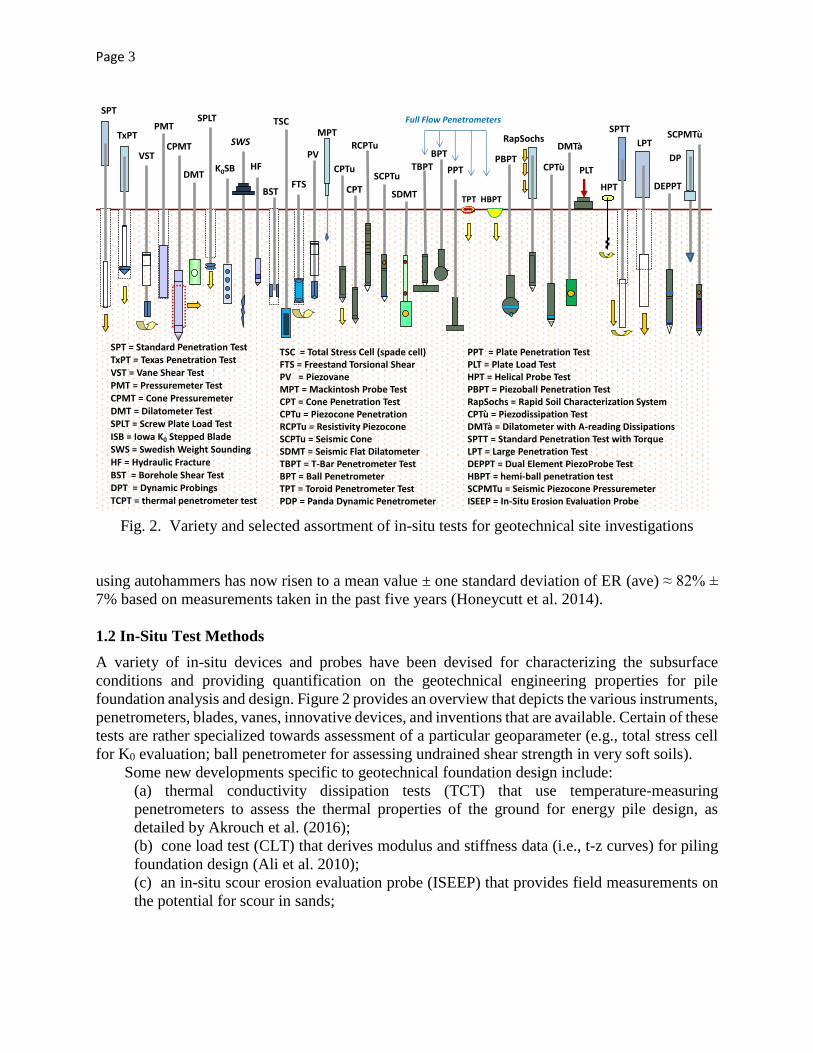
Fig. 2. Variety and selected assortment of in-situ tests for geotechnical site investigations

using autohammers has now risen to a mean value ± one standard deviation of ER (ave) ≈ 82% ±

7% based on measurements taken in the past five years (Honeycutt et al. 2014).

1.2 In-Situ Test Methods

A variety of in-situ devices and probes have been devised for characterizing the subsurface

conditions and providing quantification on the geotechnical engineering properties for pile

foundation analysis and design. Figure 2 provides an overview that depicts the various instruments,

penetrometers, blades, vanes, innovative devices, and inventions that are available. Certain of these

tests are rather specialized towards assessment of a particular geoparameter (e.g., total stress cell

for K0 evaluation; ball penetrometer for assessing undrained shear strength in very soft soils).

Some new developments specific to geotechnical foundation design include:

(a) thermal conductivity dissipation tests (TCT) that use temperature-measuring

penetrometers to assess the thermal properties of the ground for energy pile design, as

detailed by Akrouch et al. (2016);

(b) cone load test (CLT) that derives modulus and stiffness data (i.e., t-z curves) for piling

foundation design (Ali et al. 2010);

(c) an in-situ scour erosion evaluation probe (ISEEP) that provides field measurements on

the potential for scour in sands;

SPT

TxPTLPT

VST

PMT

CPMT

DMT

SPLT

K0SB

SWS

HF

BST

TSC

FTS

CPTu

CPT

RCPTu

SCPTu

SDMT

TBPT

BPT

Full Flow PenetrometersSPTT

SCPMTù

SPT = Standard Penetration TestTxPT = Texas Penetration TestVST = Vane Shear TestPMT = Pressuremeter TestCPMT = Cone PressuremeterDMT = Dilatometer TestSPLT = Screw Plate Load TestISB = Iowa K0 Stepped BladeSWS = Swedish Weight SoundingHF = Hydraulic FractureBST = Borehole Shear TestDPT = Dynamic ProbingsTCPT = thermal penetrometer test

TSC = Total Stress Cell (spade cell)FTS = Freestand Torsional ShearPV = PiezovaneMPT = Mackintosh Probe TestCPT = Cone Penetration TestCPTu = Piezocone PenetrationRCPTu = Resistivity PiezoconeSCPTu = Seismic ConeSDMT = Seismic Flat DilatometerTBPT = T-Bar Penetrometer TestBPT = Ball PenetrometerTPT = Toroid Penetrometer Test PDP = Panda Dynamic Penetrometer

PPT = Plate Penetration TestPLT = Plate Load TestHPT = Helical Probe TestPBPT = Piezoball Penetration TestRapSochs = Rapid Soil Characterization SystemCPTù = Piezodissipation TestDMTà = Dilatometer with A-reading DissipationsSPTT = Standard Penetration Test with TorqueLPT = Large Penetration TestDEPPT = Dual Element PiezoProbe TestHBPT = hemi-ball penetration testSCPMTu = Seismic Piezocone PressuremeterISEEP = In-Situ Erosion Evaluation Probe

PLT

DEPPTHPT

Selection of In-Situ Geotechnical Tests

PPT

MPT

PV PBPT

RapSochs

CPTù

DMTà

TPT HBPT

DP

Page 4

(d) multi-piezo-friction penetrometer (MPFP) for measuring soil-pile roughness and

quantification of soil-structure interaction effects on a site-specific basis (Hebeler and Frost

2006).

(e) parallel seismic method (PSM) for determining the unknown lengths of existing pile

foundations, often needed in bridge replacement or retrofit projects (Niederleithinger 2012).

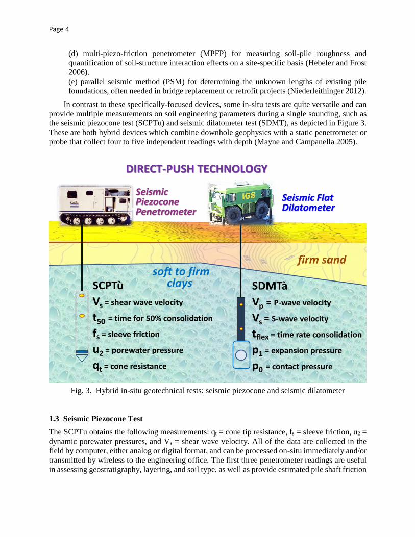
In contrast to these specifically-focused devices, some in-situ tests are quite versatile and can

provide multiple measurements on soil engineering parameters during a single sounding, such as

the seismic piezocone test (SCPTu) and seismic dilatometer test (SDMT), as depicted in Figure 3.

These are both hybrid devices which combine downhole geophysics with a static penetrometer or

probe that collect four to five independent readings with depth (Mayne and Campanella 2005).

Fig. 3. Hybrid in-situ geotechnical tests: seismic piezocone and seismic dilatometer

1.3 Seismic Piezocone Test

The SCPTu obtains the following measurements: qt = cone tip resistance, fs = sleeve friction, u2 =

dynamic porewater pressures, and Vs = shear wave velocity. All of the data are collected in the

field by computer, either analog or digital format, and can be processed on-situ immediately and/or

transmitted by wireless to the engineering office. The first three penetrometer readings are useful

in assessing geostratigraphy, layering, and soil type, as well as provide estimated pile shaft friction

DIRECT-PUSH TECHNOLOGY

SDMTà

Vp = P-wave velocity

Vs = S-wave velocity

tflex = time rate consolidation

p1 = expansion pressure

p0 = contact pressure

SCPTù

Vs = shear wave velocity

t50 = time for 50% consolidation

fs = sleeve friction

u2 = porewater pressure

qt = cone resistance

firm sandsoft to firm

clays

SeismicPiezoconePenetrometer

Seismic FlatDilatometer

Page 5

and end-bearing resistances. Of additional value, the shear wave velocity provides a fundamental

stiffness of the ground via:

G0 = Gmax = t ∙Vs2 (1)

where G0 = initial tangent shear modulus and t = t/ga = total soil mass density, t = soil unit

weight, and ga = 9.81 m/s2 = gravitational constant. This is particularly important in calculations

involving the evaluation of pile displacements and axial load transfer distributions along the pile

length.

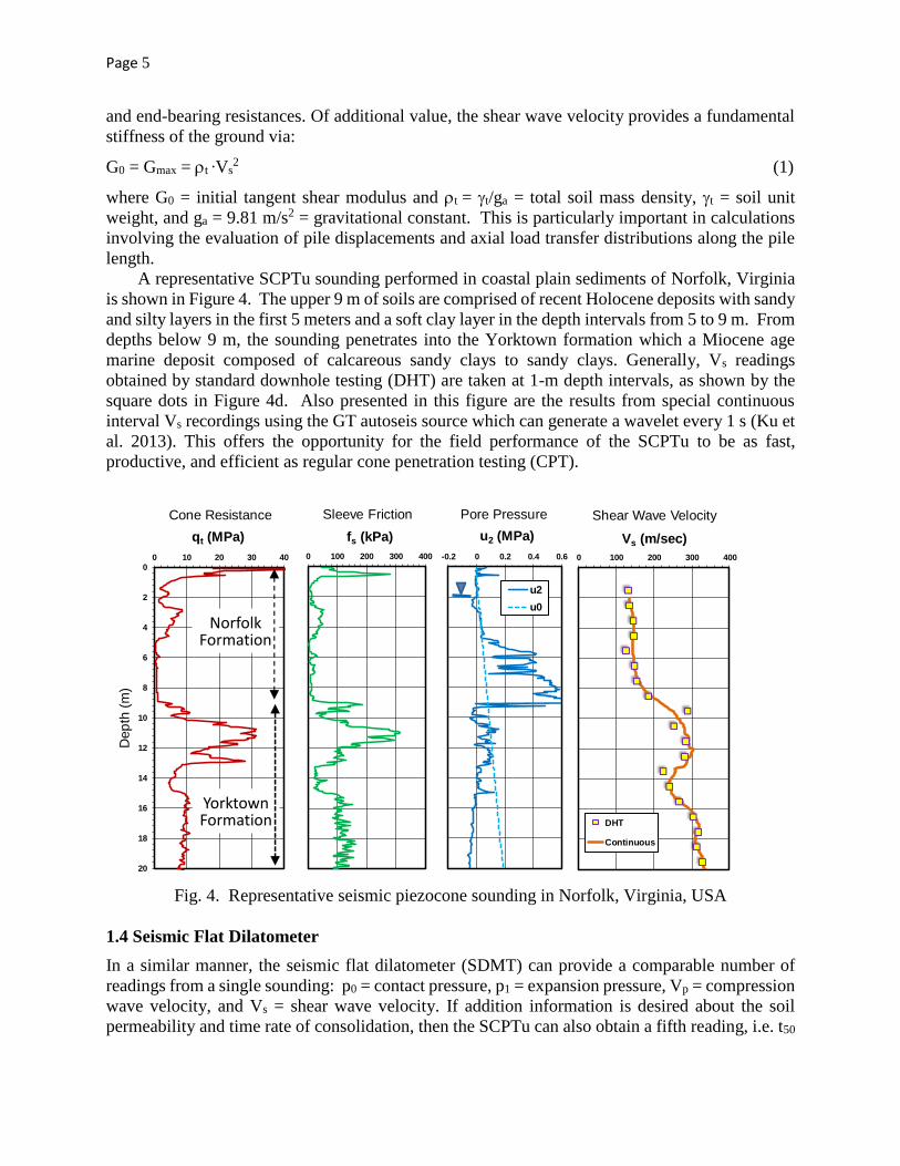
A representative SCPTu sounding performed in coastal plain sediments of Norfolk, Virginia

is shown in Figure 4. The upper 9 m of soils are comprised of recent Holocene deposits with sandy

and silty layers in the first 5 meters and a soft clay layer in the depth intervals from 5 to 9 m. From

depths below 9 m, the sounding penetrates into the Yorktown formation which a Miocene age

marine deposit composed of calcareous sandy clays to sandy clays. Generally, Vs readings

obtained by standard downhole testing (DHT) are taken at 1-m depth intervals, as shown by the

square dots in Figure 4d. Also presented in this figure are the results from special continuous

interval Vs recordings using the GT autoseis source which can generate a wavelet every 1 s (Ku et

al. 2013). This offers the opportunity for the field performance of the SCPTu to be as fast,

productive, and efficient as regular cone penetration testing (CPT).

Fig. 4. Representative seismic piezocone sounding in Norfolk, Virginia, USA

1.4 Seismic Flat Dilatometer

In a similar manner, the seismic flat dilatometer (SDMT) can provide a comparable number of

readings from a single sounding: p0 = contact pressure, p1 = expansion pressure, Vp = compression

wave velocity, and Vs = shear wave velocity. If addition information is desired about the soil

permeability and time rate of consolidation, then the SCPTu can also obtain a fifth reading, i.e. t50

0

2

4

6

8

10

12

14

16

18

20

0 10 20 30 40

Dep

th (

m)

qt (MPa)

Cone Resistance

0 100 200 300 400

fs (kPa)

Sleeve Friction

-0.2 0 0.2 0.4 0.6

u2 (MPa)

Pore Pressure

u2

u0

0 100 200 300 400

Vs (m/sec)

Shear Wave Velocity

DHT

Continuous

NorfolkFormation

YorktownFormation

Page 6

= time rate of porewater dissipation, and the SDMT can collect tflex = time rate of the p0 reading.

Example results from SDMT are presented by Marchetti et al. (2008) and Amoroso et al. (2014).

2 INTERPRETATION OF CONE PENETRATION TESTS

2.1 Geoparameter Evaluation from CPTu

The interpretation of cone and piezocone penetration tests can be made on the basis of theoretical,

analytical, numerical, empirical, and statistical relationships (Lunne et al. 1997; Mayne 2007;

Schnaid 2009). Efforts at calibration of the interpretative CPT procedures rely on one or more of

the following: (a) matching field results with benchmark values obtained from laboratory tests on

undisturbed samples, (b) backcalculating parameters from full-scale foundation performance, (c)

1-g model testing in chambers; and (d) centrifuge testing using mini- and micro-penetrometers.

Advantages and shortcomings are associated with each of these approaches.

For evaluating the axial capacity of deep foundations, the CPTu must evaluate the following

geoparameters: (a) soil type; (b) unit weight; (c) effective friction angle; (d) stress history; (e)

undrained shear strength; and (f) lateral stress coefficient. Moreover, in assessing pile

displacements and axial load distributions, the small strain shear modulus (G0 = Gmax) plays an

important role. Each of these are briefly discussed in subsequent sections, as restricted to

uncemented sands and clays of low to medium sensitivities.

2.2. Soil Behavioral Type

Since soil samples are not normally collected during CPT, indirect methods for soil classification

are often used. These generally include: (a) approximate "rules of thumb"; (b) soil behavioral type

charts; and (c) probabilistic methods. The approximate rules suggest that sands are identified when

qt > 5 MPa and u2 ≈ u0, whereas intact clays occur when qt < 5 MPa and u2 > u0 (Mayne et al.

2002). For fissured overconsolidated clays, u2 readings are often negative. Probability-based

methods are discussed by Tumay et al. (2013).

The most popular methods are based on soil behavioral charts with popular favoring of the 9-

zone classification system (Lunne et al. 1997; 2009) that uses normalized piezocone readings: (a)

normalized tip resistance: Q = (qt - vo)/vo', (b) normalized sleeve friction: F (%) = 100∙fs/(qt -

vo); and normalized porewater pressure: Bq = (u2 - u0)/(qt - vo). Any of these indirect CPT soil

classification approaches should be cross-checked and verified for a particular geologic setting

before routine use in practice.

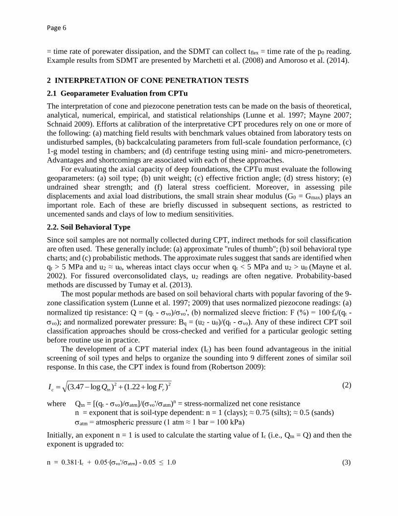
The development of a CPT material index (Ic) has been found advantageous in the initial

screening of soil types and helps to organize the sounding into 9 different zones of similar soil

response. In this case, the CPT index is found from (Robertson 2009):

(2)

where Qtn = [(qt - vo)/atm]/(vo'/atm)n = stress-normalized net cone resistance

n = exponent that is soil-type dependent: n = 1 (clays); ≈ 0.75 (silts); ≈ 0.5 (sands)

atm = atmospheric pressure (1 atm ≈ 1 bar = 100 kPa)

Initially, an exponent n = 1 is used to calculate the starting value of Ic (i.e., Qtn = Q) and then the

exponent is upgraded to:

n = 0.381∙Ic + 0.05∙(vo'/atm) - 0.05 ≤ 1.0 (3)

22 )log22.1()log47.3( rtnc FQI

Page 7

Fig. 5. Soil behavioral type zones and algorithms for zone identification by CPT

Then the index Ic is recalculated. Iteration converges quickly and generally only 3 cycles are

needed to secure the operational Ic at each depth. The soil zones and associated Ic values are

detailed in Figure 5. The sensitive soils of zone 1 can be screened using the following expression:

Zone 1: Qtn < 12 exp ( -1.4 ∙ Fr) (4)

The stiff soils of zone 8 (1.5% < Fr < 4.5%) and zone 9 (Fr > 4.5%) can be identified from:

Zones 8 and 9: 002.0)1(0003.0)1(005.0

12

rr

tnFF

Q (5)

Then, the remaining soil types are identified by the CPT material index: Zone 2 (organic clayey

soils: Ic ≥ 3.60); Zone 3 (clays to silty clays: 2.95 ≤ Ic < 3.60); Zone 4 (silt mixtures: 2.60 ≤ Ic <

2.95); Zone 5 (sand mixtures: 2.05 ≤ Ic < 2.60); Zone 6 (clean sands: 1.31 ≤ Ic < 2.05); and Zone

7 (gravelly to dense sands: Ic ≤ 1.31). The red dashed line at Ic = 2.60 represents an approximate

boundary separating drained (Ic < 2.60) from undrained behavior (Ic > 2.60).

2.3. Soil Unit Weight

Soil unit weight can be estimated from the CPT sleeve friction resistance (Mayne 2015):

Soil BehavioralType (SBTn) Chartfor normalized CPT

(after Robertson 2009)

1

10

100

1000

0.1 1 10

Norm

aliz

ed T

ip R

esis

tan

ce,

Qtn

Normalized Friction, Fr = 100 fs /(qt - vo) (%)

9 - ZONE SBT

Gravelly Sands (zone 7)

Sands(zone 6)

Sandy Mixtures(zone 5)

Silt Mix(zone 4)

Clays(zone 3)

Organic Soils(zone 2)

FocalPoint

Sensitive Claysand Silts(zone 1)

Ic = 1.31

Ic = 2.05

Ic = 2.60

Ic = 2.95

Ic = 3.60

Notes:

Ic = Radius:

Very stiff OC clayto silt (zone 9)

n

atmvo

atmvottn

qQ

)/'(

/)(

22 )log22.1()log47.3( rtnc FQI

Very stiffOC sandto clayey

sand(zone 8)

Exponent: 15.0)/'(05.0381.0 atmvocIn

a. Find sensitive soils of zone 1 identified when: Qtn < 12 exp(-1.4 Fr )

b. Identify: Zone 8 (1.5 < Fr< 4.5%) and Zone 9 (Fr > 4.5%):

c. Use CPT index Ic for Zones 2 through 7 002.0)9.0(0004.0)9.0(006.0

12

rr

tnFF

Q

ApproximateAlgorithm Steps:

Ic < 2.6: Drained

Ic > 2.6: Undrained

Page 8

t/w = 1.22 + 0.15 ∙ ln (100*fs/atm+0.01) (6)

where w = unit weight of water.

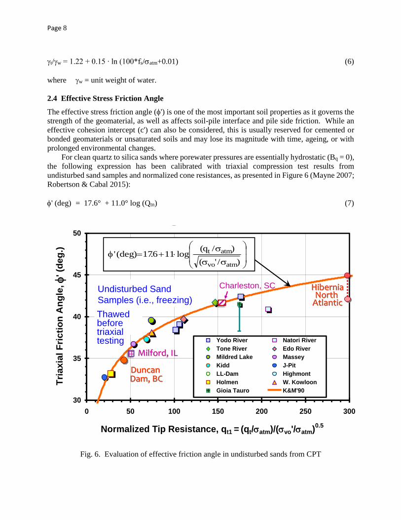
2.4 Effective Stress Friction Angle

The effective stress friction angle (') is one of the most important soil properties as it governs the

strength of the geomaterial, as well as affects soil-pile interface and pile side friction. While an

effective cohesion intercept (c') can also be considered, this is usually reserved for cemented or

bonded geomaterials or unsaturated soils and may lose its magnitude with time, ageing, or with

prolonged environmental changes.

For clean quartz to silica sands where porewater pressures are essentially hydrostatic (Bq = 0),

the following expression has been calibrated with triaxial compression test results from

undisturbed sand samples and normalized cone resistances, as presented in Figure 6 (Mayne 2007;

Robertson & Cabal 2015):

' (deg) = 17.6° + 11.0° log (Qtn) (7)

Fig. 6. Evaluation of effective friction angle in undisturbed sands from CPT

Friction Angle of Sands from CPT

30

35

40

45

50

0 50 100 150 200 250 300

Normalized Tip Resistance, qt1 = (qt/atm)/(vo'/atm)0.5

Tri

axia

l F

ric

tio

n A

ng

le,

' (d

eg

.)

Yodo River Natori River

Tone River Edo River

Mildred Lake Massey

Kidd J-Pit

LL-Dam Highmont

Holmen W. Kowloon

Gioia Tauro K&M'90

)/'(

)/q(log116.17(deg)'

atmvo

atmt

Sands with mica, smectite, illite,

and other minerals

DuncanDam, BC

HiberniaNorth

Atlantic

Milford, IL

Charleston, SCUndisturbed Sand

Samples (i.e., freezing)

Thawedbefore triaxialtesting

Page 9

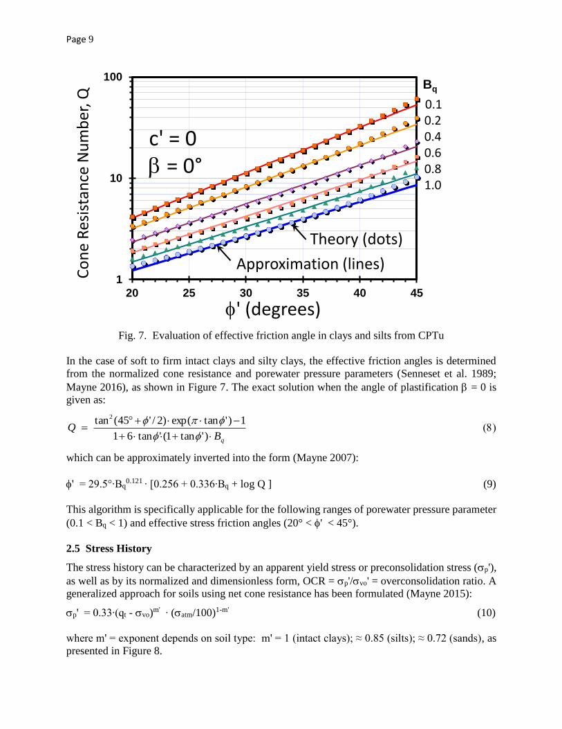
Fig. 7. Evaluation of effective friction angle in clays and silts from CPTu

In the case of soft to firm intact clays and silty clays, the effective friction angles is determined

from the normalized cone resistance and porewater pressure parameters (Senneset et al. 1989;

Mayne 2016), as shown in Figure 7. The exact solution when the angle of plastification = 0 is

given as:

qBQ

)'tan1('tan61

1)'tanexp()2/'45(tan2

which can be approximately inverted into the form (Mayne 2007):

' = 29.5°∙Bq0.121 ∙ [0.256 + 0.336∙Bq + log Q ] (9)

This algorithm is specifically applicable for the following ranges of porewater pressure parameter

(0.1 < Bq < 1) and effective stress friction angles (20° < ' < 45°).

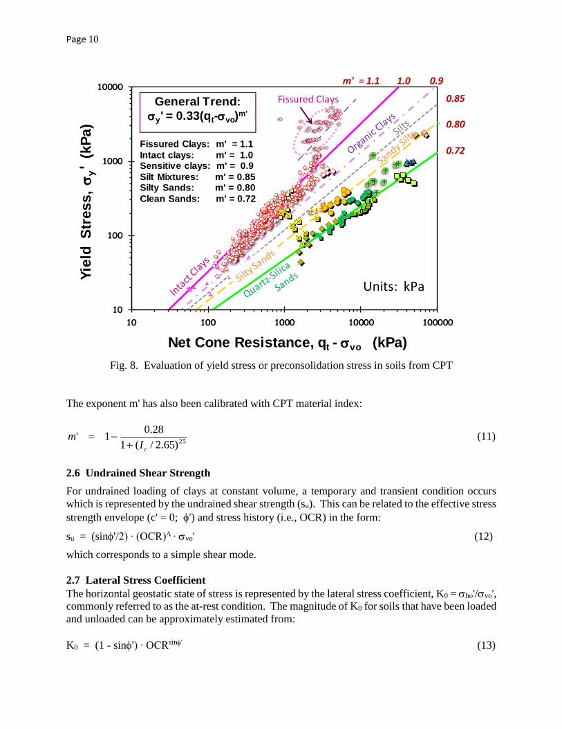
2.5 Stress History

The stress history can be characterized by an apparent yield stress or preconsolidation stress (p'),

as well as by its normalized and dimensionless form, OCR = p'/vo' = overconsolidation ratio. A

generalized approach for soils using net cone resistance has been formulated (Mayne 2015):

p' = 0.33∙(qt - vo)m' ∙ (atm/100)1-m' (10)

where m' = exponent depends on soil type: m' = 1 (intact clays); ≈ 0.85 (silts); ≈ 0.72 (sands), as

presented in Figure 8.

Approximate NTH Solution for ' from CPTu

qBQ

)'tan1('tan61

1)'tanexp()2/'45(tan2

Approx: ' ≈ 29.5°∙Bq0.121∙[0.256 + 0.336∙Bq + log Q ]

1

10

100

20 25 30 35 40 45

Co

ne

Res

ista

nce

Nu

mb

er, Q

' (degrees)

Bq

0.10.20.40.60.81.0

c' = 0 = 0°

Theory (dots)

Approximation (lines)

Theory:

Page 10

Fig. 8. Evaluation of yield stress or preconsolidation stress in soils from CPT

The exponent m' has also been calibrated with CPT material index:

25)65.2/(1

28.01'

cIm

(11)

2.6 Undrained Shear Strength

For undrained loading of clays at constant volume, a temporary and transient condition occurs

which is represented by the undrained shear strength (su). This can be related to the effective stress

strength envelope (c' = 0; ') and stress history (i.e., OCR) in the form:

su = (sin'/2) ∙ (OCR)∙ vo' (12)

which corresponds to a simple shear mode.

2.7 Lateral Stress Coefficient

The horizontal geostatic state of stress is represented by the lateral stress coefficient, K0 = ho'/vo',

commonly referred to as the at-rest condition. The magnitude of K0 for soils that have been loaded

and unloaded can be approximately estimated from:

K0 = (1 - sin') ∙ OCRsin' (13)

Yield stress in soils from CPT

10

100

1000

10000

10 100 1000 10000 100000

Yie

ld S

tre

ss

,

y'

(kP

a)

Net Cone Resistance, qt - vo (kPa)

Blessington

General Trend:

y' = 0.33(qt-vo)m'

Fissured Clays: m' = 1.1

Intact clays: m' = 1.0 Sensitive clays: m' = 0.9

Silt Mixtures: m' = 0.85Silty Sands: m' = 0.80

Clean Sands: m' = 0.72

m' = 1.1 1.0 0.9

0.85

0.80

0.72

Units: kPa

Fissured Clays

Page 11

The value of K0 finds applicability in assessing the pile side friction via the beta method, whereby

as a first approximation: = K0 ∙ tan'.

2.8 Additional GeoParameters

If desired, additional engineering properties can be determined during SCPTu (e.g., Robertson and

Cabal 2015). For instance, the effective cohesion intercept (c') can also be determined from

plotting (qt - vo) versus vo' (Mayne 2016). If piezo-dissipation measurements are taken, the

coefficient of consolidation (cvh) and permeability (k) can be assessed (Mayne and Campanella

2005). This can be useful for pile driving projects in clays and silts that require an estimate of time

for equilibrium of excess porewater pressures caused during installation, as well as for ground

modification projects where these data are used for calculating time-rate-of-consolidation and wick

drain spacings.

.

3 RELEVANCE OF SCPTu in DEEP FOUNDATION DESIGN

The analysis of the axial load-displacement-capacity response of deep foundations is usually

separated into two analytical components: (a) capacity; and (b) displacements. The SCPTu

provides sufficient data input to handle the requirements using conventional calculations using

limit equilibrium and plasticity solutions, as well as direct methods that are based on statistical

analyses of large foundation load test databases, most recently funded by the offshore energy

industry, including oil, gas, and wind.

3.1 Traditional Methods for Evaluating Side Friction and Toe Resistance

In common practice, pile shaft friction (rs) is often calculated using alpha methods for clays and

beta methods for sands (Brown et. al. 2010). The beta method has also shown applicable for both

clays and sands (O'Neill 2001; Fellenius 2016). Using the information from Section 2.7, a

generalized expression for shaft friction can be given by:

rs = CM ∙ CK ∙ K0 ∙ vo' ∙ tan' (14)

where CM = pile material factor = 1 (rough cast-in-place concrete); 0.9 (prestressed concrete)

0.8 (timber); and 0.7 (steel);

CK = installation factor = 0.9 (bored or augered); 1.0 (low displacement, e.g. H-pile or

open end pipe); and 1.1 (driven solid, e.g. prestressed concrete, closed-end pipe).

The evaluation of toe resistance (rt) is often taken from limit plasticity solutions with associated

shape and depth factors (Brown et al. 2010). For undrained toe response, the full value may be

attained, thus:

undrained: rt = Nc' ∙ su (15)

where Nc' = 9.33 for a circular pile.

For drained toe response, the situation is more complex as the pile toe resistance increases with

toe displacement (Fellenius 2016). Thus, from a practical standpoint, only a portion of the

theoretical resistance will be realized:

drained: rt = vo' ∙ Nq' ∙ fx' (16)

Page 12

where Nq' ≈ 0.77 ∙ exp ('/7.5°) = approximate expression for bearing factor

fx' = strain incompatibility factor = 0.1 (bored piles); 0.2 (jacked); 0.3 (driven)

3.2 Direct CPT methods for Axial Pile Capacity

In lieu of assessing soil parameters (t', su, K0, OCR) from CPT results that are input into

theoretical formulae, considerable research efforts have centered on Direct CPT methods whereby

the measured CPT results are scaled straightaway to provide unit shaft (rs) and unit toe (rt)

resistances. At least 35 different Direct CPT methods are available (Niazi and Mayne 2013).

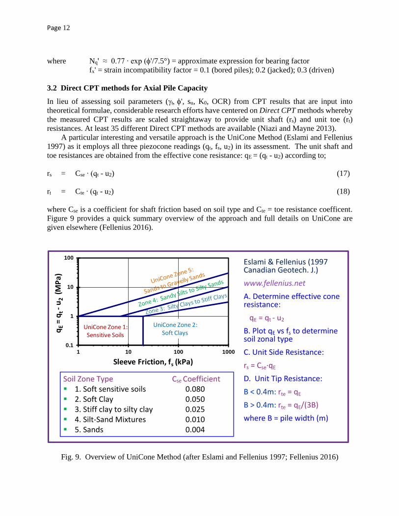
A particular interesting and versatile approach is the UniCone Method (Eslami and Fellenius

1997) as it employs all three piezocone readings (qt, fs, u2) in its assessment. The unit shaft and

toe resistances are obtained from the effective cone resistance: qE = (qt - u2) according to;

rs = Cse ∙ (qt - u2) (17)

rt = Cte ∙ (qt - u2) (18)

where Cse is a coefficient for shaft friction based on soil type and Cte = toe resistance coefficent.

Figure 9 provides a quick summary overview of the approach and full details on UniCone are

given elsewhere (Fellenius 2016).

Fig. 9. Overview of UniCone Method (after Eslami and Fellenius 1997; Fellenius 2016)

Overview: UniCone CPTu Method

Soil Zone Type Cse Coefficient 1. Soft sensitive soils 0.080 2. Soft Clay 0.050 3. Stiff clay to silty clay 0.025 4. Silt-Sand Mixtures 0.010 5. Sands 0.004

Eslami & Fellenius (1997 Canadian Geotech. J.)

www.fellenius.net

A. Determine effective cone resistance:

qE = qt - u2

B. Plot qE vs fs to determine soil zonal type

C. Unit Side Resistance:

rs = Cse∙qE

D. Unit Tip Resistance:

B < 0.4m: rte = qE

B > 0.4m: rte = qE/(3B)

where B = pile width (m)

fs (kPa)

0.1

1

10

100

1 10 100 1000

qE

= q

t -

u2

(MP

a)

Sleeve Friction, fs (kPa)

UniCone Zone 1:Sensitive Soils

UniCone Zone 2:Soft Clays

Page 13

A modified UniCone approach has been devised that uses the CPT material index (Ic) to assign

values to the Cse and Cte coefficients (Niazi and Mayne 2016). For SBTn zone 1 (sensitive clays),

the Cse coefficient is obtained from:

SBTn Zone 1: Cse = 0.074 - 0.004 ∙ [Qtn - 12 ∙ exp(-1.4∙F)] (19)

and for the remaining soil types, the shaft coefficient may be estimated from the following

expression:

SBTn Zones 2 to 9: Cse = 1 ∙ 2 ∙ 3 ∙ 10 [0.732∙Ic - 3.605] (20)

where 1 = pile type factor: 0.84 (bored piles), 1.02 (jacked), 1.13 (driven); 2 = load direction

factor: 1.11 (compression) and 0.85 (tension), and 3 = loading rate factor (1.0 for soils with Ic <

2.6 and for Ic > 2.6: 0.97 (stepped load) and 1.09 (constant rate of penetration).

The toe coefficient may be estimated from:

All SBTn Zones: Cte = 10 [0.325∙Ic - 1.218] (21)

The total axial compression capacity (Qult) is the sum of shaft capacity (Rs) plus toe capacity (Rt):

Qult = Rs + Rt = ∫ (As ∙ rs) dz + At ∙ rt (22)

where As = circumferential area of the pile at depth z and At = toe area of the pile.

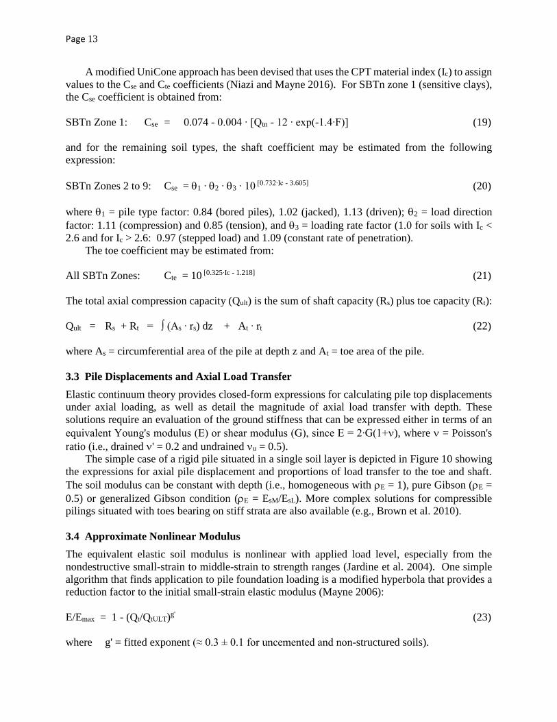
3.3 Pile Displacements and Axial Load Transfer

Elastic continuum theory provides closed-form expressions for calculating pile top displacements

under axial loading, as well as detail the magnitude of axial load transfer with depth. These

solutions require an evaluation of the ground stiffness that can be expressed either in terms of an

equivalent Young's modulus (E) or shear modulus (G), since E = 2∙G(1+), where = Poisson's

ratio (i.e., drained ' = 0.2 and undrained u = 0.5).

The simple case of a rigid pile situated in a single soil layer is depicted in Figure 10 showing

the expressions for axial pile displacement and proportions of load transfer to the toe and shaft.

The soil modulus can be constant with depth (i.e., homogeneous with E = 1), pure Gibson (E =

0.5) or generalized Gibson condition (E = EsM/EsL). More complex solutions for compressible

pilings situated with toes bearing on stiff strata are also available (e.g., Brown et al. 2010).

3.4 Approximate Nonlinear Modulus

The equivalent elastic soil modulus is nonlinear with applied load level, especially from the

nondestructive small-strain to middle-strain to strength ranges (Jardine et al. 2004). One simple

algorithm that finds application to pile foundation loading is a modified hyperbola that provides a

reduction factor to the initial small-strain elastic modulus (Mayne 2006):

E/Emax = 1 - (Qt/QtULT)g' (23)

where g' = fitted exponent (≈ 0.3 ± 0.1 for uncemented and non-structured soils).

Page 14

Fig. 10. Elastic continuum solution for rigid axial pile in soil layer

The seismic piezocone test (SCPTu) thus finds special application to deep foundation analysis

because it provides sufficient data (qt, fs, and u2) for axial pile capacity calculations, as well as

supplying the necessary soil stiffness (Emax) for the evaluation of displacements and load transfer.

To illustrate the usefulness of the SCPTu results in axial pile evaluation, a case study from load

tests for the Wakota Bridge are presented.

4 CASE STUDY - WAKOTA BRIDGE, MINNESOTA

The ten-lane Wakota Bridge is located southeast of Saint Paul, Minnesota and was completed in

2010. The bridge enables interstate loop 494 to cross the Mississippi River. During the design

phase, load tests on both driven open-end and closed end steel pipe piles were conducted with test

piles having an outer diameter d = 0.457 m, an embedded length L = 32 m, and wall thickness t =

12.5 mm (Dasenbrock 2006). Both piles were loaded in axial compression, then afterwards loaded

in tension, using a static reaction frame arrangement.

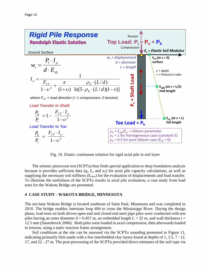
Soil conditions at the site can be assessed via the SCPTu sounding presented in Figure 11,

indicating primarily firm sands with a few interbedded clay layers found at depths of 1, 3.5, 7 - 12,

17, and 22 - 27 m. The post-processing of the SCPTu provided direct estimates of the soil type via

Ps

= Sh

aft

Load

sL

t

tEd

IPw

Load Transfer to Toe:

)]1)(/(5ln[

)/(

)1(1

1

2 vdL

dLFI

E

ECT

211

IF

P

P CT

t

b

Toe Load = Pb

Randolph Elastic Solution

Ground Surface

Top Load: Pt = Ps + Pb

Rigid Pile Response

wt = displacementd = diameter

L = length

Es = Elastic Soil Modulus

Es0 (at z = 0)surface

EsM (at z = L/2)mid-length

EsL (at z = L)full length

Load Transfer to Shaft:

E = EsM/EsL = Gibson parameterE = 1 for homogeneous case (constant E)E = 0.5 for pure Gibson case (Es0 = 0)

where FCT = load direction (= 1 compression; 0 tension)

21

IF

P

P CT

t

b

z = depth

= Poisson's ratio

Tension

Compression

Page 15

Fig. 11. Seismic piezocone results at I-494 Wakota Bridge site, Saint Paul, Minnesota

material index (Ic), unit weight (t), effective friction angle ('), preconsolidation stress (p'), and

K0 profiles for input into beta method for pile shaft resistance (ave. rs = 65 kPa), as well as by

direct CPT methods using Unicone (ave. rs = 70 kPa) and Modified Unicone (ave. rs = 75 kPa).

Evaluation of the toe resistance determined rte = 3593 kPa by the Modified Unicone expression.

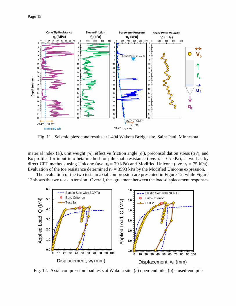
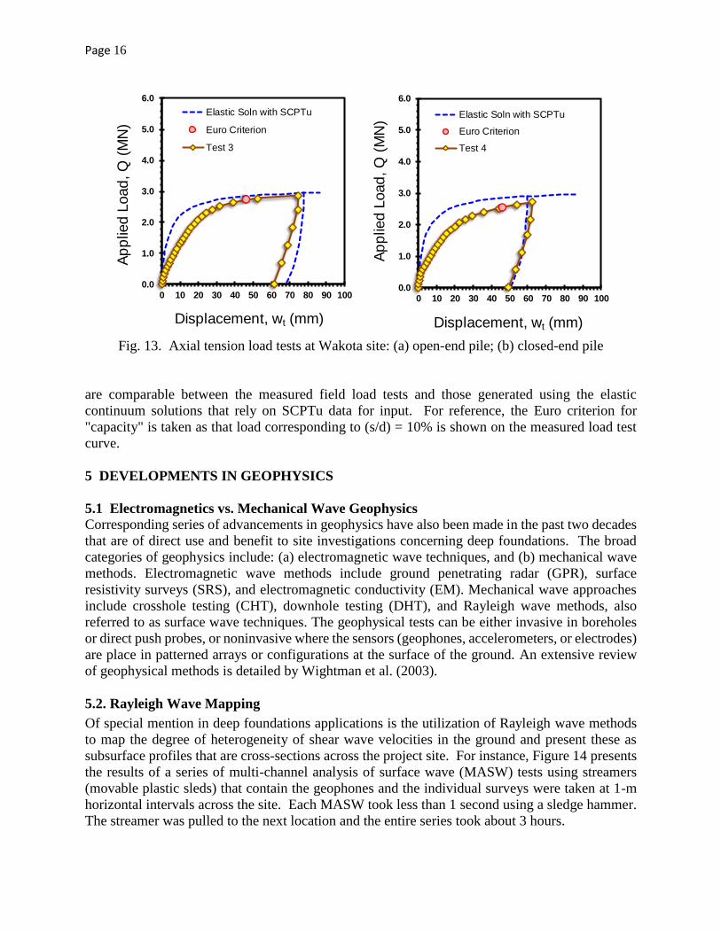
The evaluation of the two tests in axial compression are presented in Figure 12, while Figure

13 shows the two tests in tension. Overall, the agreement between the load-displacement responses

Fig. 12. Axial compression load tests at Wakota site: (a) open-end pile; (b) closed-end pile

MnDOT Wakota Bridge - CPTu C107

0

2

4

6

8

10

12

14

16

18

20

22

24

26

28

30

32

34

36

0 5 10 15 20 25 30 35 40

De

pth

(m

ete

rs)

Cone Tip Resistance

qt (MPa)

qt

u2

fs

CLAY SAND

5 MPa (50 tsf)

VS

0

2

4

6

8

10

12

14

16

18

20

22

24

26

28

30

32

34

36

0 100 200 300 400

Sleeve Friction

fs (kPa)

0

2

4

6

8

10

12

14

16

18

20

22

24

26

28

30

32

34

36

0 200 400 600 800 1000

Porewater Pressure

u2 (kPa)

INTACT CLAY:u2 > u0

SAND: u2 ≈ u0

Groundwater at 9.0 m

0

2

4

6

8

10

12

14

16

18

20

22

24

26

28

30

32

34

36

0 100 200 300 400

Shear Wave Velocity

Vs (m/s)

0

2

4

6

8

10

12

14

16

18

20

22

24

26

28

30

32

34

36

0 100 200 300 400

Shear Wave Velocity

Vs (m/s)

Wakota Bridge

0.050

0.100

0.150

0.200

0.250

0.300

0.350

0.400

0.450

0.500

0.550

0.600

0.650

0.700

0.0

1.0

2.0

3.0

4.0

5.0

6.0

0 10 20 30 40 50 60 70 80 90 100

Ap

plie

d L

oad

, Q

(M

N)

Displacement, wt (mm)

Elastic Soln with SCPTu

Euro Criterion

Test 1a

0.0

1.0

2.0

3.0

4.0

5.0

6.0

0 10 20 30 40 50 60 70 80 90 100

Ap

plie

d L

oad

, Q

(M

N)

Displacement, wt (mm)

Elastic Soln with SCPTu

Euro Criterion

Test 2

Page 16

Fig. 13. Axial tension load tests at Wakota site: (a) open-end pile; (b) closed-end pile

are comparable between the measured field load tests and those generated using the elastic

continuum solutions that rely on SCPTu data for input. For reference, the Euro criterion for

"capacity" is taken as that load corresponding to (s/d) = 10% is shown on the measured load test

curve.

5 DEVELOPMENTS IN GEOPHYSICS

5.1 Electromagnetics vs. Mechanical Wave Geophysics

Corresponding series of advancements in geophysics have also been made in the past two decades

that are of direct use and benefit to site investigations concerning deep foundations. The broad

categories of geophysics include: (a) electromagnetic wave techniques, and (b) mechanical wave

methods. Electromagnetic wave methods include ground penetrating radar (GPR), surface

resistivity surveys (SRS), and electromagnetic conductivity (EM). Mechanical wave approaches

include crosshole testing (CHT), downhole testing (DHT), and Rayleigh wave methods, also

referred to as surface wave techniques. The geophysical tests can be either invasive in boreholes

or direct push probes, or noninvasive where the sensors (geophones, accelerometers, or electrodes)

are place in patterned arrays or configurations at the surface of the ground. An extensive review

of geophysical methods is detailed by Wightman et al. (2003).

5.2. Rayleigh Wave Mapping

Of special mention in deep foundations applications is the utilization of Rayleigh wave methods

to map the degree of heterogeneity of shear wave velocities in the ground and present these as

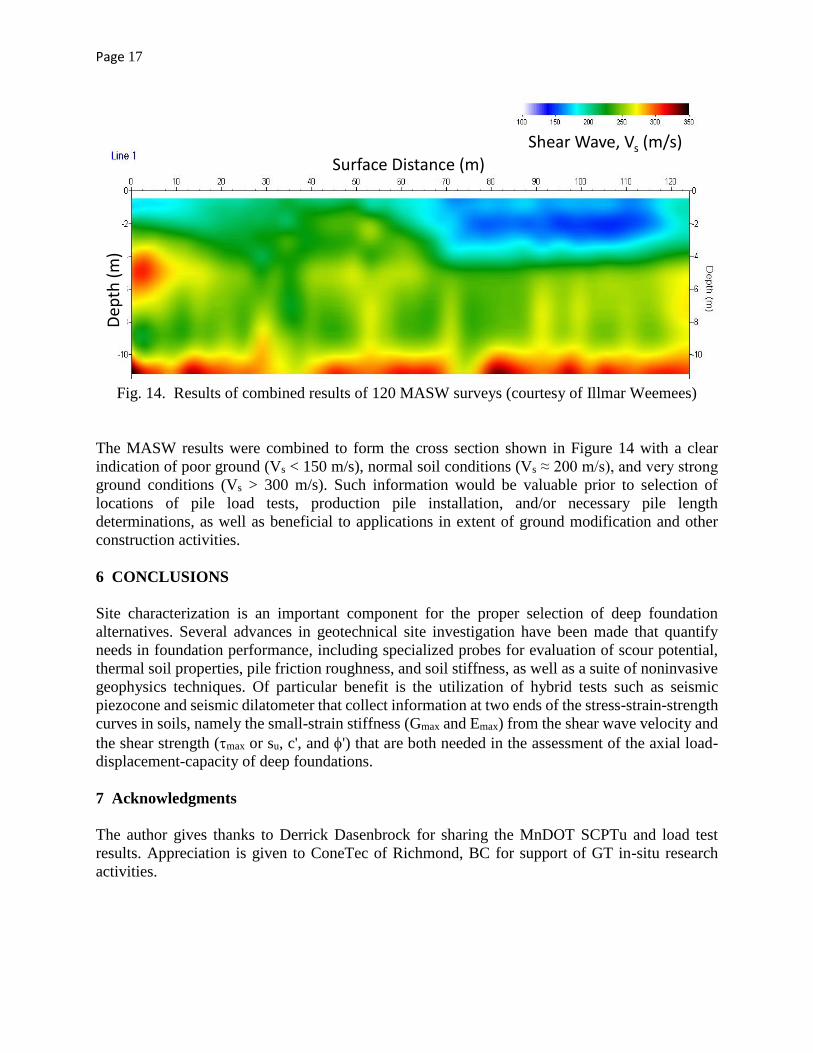
subsurface profiles that are cross-sections across the project site. For instance, Figure 14 presents

the results of a series of multi-channel analysis of surface wave (MASW) tests using streamers

(movable plastic sleds) that contain the geophones and the individual surveys were taken at 1-m

horizontal intervals across the site. Each MASW took less than 1 second using a sledge hammer.

The streamer was pulled to the next location and the entire series took about 3 hours.

Wakota Bridge

0.050

0.100

0.150

0.200

0.250

0.300

0.350

0.400

0.450

0.500

0.550

0.600

0.650

0.700

0.750

0.0

1.0

2.0

3.0

4.0

5.0

6.0

0 10 20 30 40 50 60 70 80 90 100

Ap

plie

d L

oad

, Q

(M

N)

Displacement, wt (mm)

Elastic Soln with SCPTu

Euro Criterion

Test 3

0.0

1.0

2.0

3.0

4.0

5.0

6.0

0 10 20 30 40 50 60 70 80 90 100

Ap

plie

d L

oad

, Q

(M

N)

Displacement, wt (mm)

Elastic Soln with SCPTu

Euro Criterion

Test 4

Page 17

Fig. 14. Results of combined results of 120 MASW surveys (courtesy of Illmar Weemees)

The MASW results were combined to form the cross section shown in Figure 14 with a clear

indication of poor ground (Vs < 150 m/s), normal soil conditions (Vs ≈ 200 m/s), and very strong

ground conditions (Vs > 300 m/s). Such information would be valuable prior to selection of

locations of pile load tests, production pile installation, and/or necessary pile length

determinations, as well as beneficial to applications in extent of ground modification and other

construction activities.

6 CONCLUSIONS

Site characterization is an important component for the proper selection of deep foundation

alternatives. Several advances in geotechnical site investigation have been made that quantify

needs in foundation performance, including specialized probes for evaluation of scour potential,

thermal soil properties, pile friction roughness, and soil stiffness, as well as a suite of noninvasive

geophysics techniques. Of particular benefit is the utilization of hybrid tests such as seismic

piezocone and seismic dilatometer that collect information at two ends of the stress-strain-strength

curves in soils, namely the small-strain stiffness (Gmax and Emax) from the shear wave velocity and

the shear strength (max or su, c', and ') that are both needed in the assessment of the axial load-

displacement-capacity of deep foundations.

7 Acknowledgments

The author gives thanks to Derrick Dasenbrock for sharing the MnDOT SCPTu and load test

results. Appreciation is given to ConeTec of Richmond, BC for support of GT in-situ research

activities.

Combined MASW Arrays for 2DMapping Subsurface Heterogeneity

Surface Distance (m)Shear Wave, Vs (m/s)

Dep

th (

m)

courtesy: Illmar Weemees - ConeTec

Page 18

8 References

Akrouch, G.A., Briaud, J-L., Sanchez, M. and Yilmaz, R. 2016. Thermal cone test to determine

soil thermal properties. J. Geotechnical & Geoenvironmental Engrg. 142 (3): 04014085.

Amoroso, S., Monaco, P., Lehane, B.M. and Marchetti, D. 2014. Examination of the potential of

the SDMT to estimate in-situ stiffness decay curves. Soils and Rocks 37 (3): 177-194.

Ali, H., Reiffsteck, P., Baguelin, F., van de Graaf, H., Bacconnet, C. and Gourvès, R. 2010.

Settlement of pile using cone loading test: load settlement curve approach. Proc. 2nd Intl.

Symp. on Cone Penetration Testing (CPT'10), Huntingdon Beach, California: Paper ID 3-24.

Brown, D.A., Turner, J.P. and Castelli, R.J. 2010. Drilled shafts: construction procedures and

LRFD design Methods. Report FHWA-NHI-10-016, National Highway Institute, Federal

Highway Administration, Washington, DC: 972 p.

Dasenbrock, D.D. 2006. Assessment of pile capacity by static and dynamic methods to reconcile

design predictions with observed performance. Proc. 54th Minnesota Geotechnical

Engineering Conference, Edited by Labuz, J., Univ. of Minnesota, St. Paul: 95-108.

Davidson, J.L., Maultsby, J.P. and Spoor, K.B. 1999. Standard penetration test energy calibrations.

Report Number WPI 0510859 by Univ. Florida - Gainesville submitted to Florida Dept.

Transportation, Tallahassee: 123 pages.

Eslami, A. and Fellenius, B.H. 1997. Pile capacity by direct CPT and CPTu methods applied to

102 case histories. Canadian Geotechnical Journal 34 (6): 886-904.

Fellenius, B.H, 2016. Basics of Foundation Design, Electronic Edition, Sidney, British Columbia,

453 pages: www.fellenius.net

Finno, R.J., Gassman, S.L. and Calvello, M. 2000. The NGES at Northwestern University.

National Geotechnical Experimentation Sites (GSP 93), ASCE, Reston, Virginia: 130-159.

Gabr, M., Caruso, C., Key, A. and Kayser, M. 2013. Assessment of in-situ scour profile in sand

using a jet probe. ASTM Geotechnical Testing J. 36 (2): 1-11.

Hebeler, G.L. and Frost, J.D. 2006. A multi-piezo-friction attachment for penetration testing.

Geotechnical Engineering in the Information Technology Age (Proc. GeoCongress, Atlanta),

ISBN 9781604234909; ASCE, Reston, Virginia: 1-6.

Honeycutt, J.N., Kiser, S.E. and Anderson, J.B. 2014. Database evaluation of energy transfer for

cme automatic hammer SPT. J. Geotechnical & Geoenv. Engrg. 140 (1): 194-200.

Jardine, R.J., Gens, A., Hight, D.W. and Coop, M.R. 2004. Developments in understanding soil

behavior. Advances in Geotechnical Engineering (Proc. Skempton Conference), Thomas

Telford, London: 103-206.

Ku, T., Mayne, P.W, and Cargill, E. 2013. Continuous-interval shear wave velocity profiling by

auto-source and seismic piezocone tests. Canadian Geotechnical J. 50 (1): 382–390.

Lunne, T., Robertson, P.K. and Powell, J.J.M. 1997. Cone Penetration Testing in Geotechnical

Practice. EF Spon/Blackie Academic, London, 352 p.

Marchetti, S., Monaco, P., Totani, G., and Marchetti, D. (2008). In-situ tests by seismic dilatometer

(SDMT). From Research to Practice in Geotechnical Engineering (Proc. GeoCongress 2008,

GSP 180, New Orleans), ASCE, Reston, Virginia: 292-311.

Mayne, P.W., Christopher, B., Berg, R., and DeJong, J. 2002. Subsurface Investigations -

Geotechnical Site Characterization. Publication No. FHWA-NHI-01-031, National Highway

Institute, Federal Highway Administration, Washington, D.C., 301 p.

Page 19

Mayne, P.W. and Campanella, R.G. 2005. Versatile site characterization by seismic piezocone

tests. Proceedings, 16th International Conference on Soil Mechanics & Geotechnical

Engineering, (ICSMGE, Osaka), Vol. 2, Millpress, Rotterdam: 721-724.

Mayne, P.W. 2007. NCHRP Synthesis 368 on Cone Penetration Test. Transportation Research

Board, National Academies Press, Washington, D.C., 118 p. www.trb.org

Mayne, P.W. 2015. Keynote lecture: In-situ geocharacterization of soils in the year 2016 and

beyond. Advances in Soil Mechanics, Vol. 5: Geotechnical Synergy (Proc. 15th PCSMGE,

Buenos Aires), IOS Press, Amsterdam: 139-161.

Mayne, P.W. 2016. Evaluating effective stress parameters and undrained shear strengths of soft-

firm clays from CPTu and DMT. Australian Geomechanics J. 51 (4): 27-55.

Niazi, F.S. and Mayne, P.W. (2013). Cone penetration test based direct methods for evaluating

static axial capacity of single piles. Geot. and Geological Engrg. 31 (4), Springer: 979-1009.

Niazi, F.S. and Mayne, P.W. (2016). CPTu-based enhanced UniCone method for pile capacity.

Engineering Geology 212, Elsevier: 21-34.

Niederleithinger, E. 2012. Improvement and extension of the parallel seismic method for

foundation depth measurement. Soils and Foundations 52 (6): 1093-1101.

O'Neill, M.W. 2001. Side resistance in piles and drilled shafts (34th Terzaghi Lecture). J.

Geotechnical & Geoenvironmental Engineering 127 (1): 3-16. Robertson, P.K. 2009. Cone penetration testing: a unified approach. Canadian Geotechnical J. 46

(11): 1337-1355. Robertson, P.K. and Cabal, K.L. 2015. Guide to Cone Penetration Testing for Geotechnical

Engineering, 6th Edition, Gregg Drilling & Testing, Inc., Signal Hill, California: 142 p. Schnaid, F. 2009. In-Situ Testing in Geomechanics: The Main Tests. Taylor & Francis Group,

London, 322 p.

Seed, H.B., Tokimatsu, K., Harder, L.F. and Chung, R.M. 1985. The influence of SPT procedures

in soil liquefaction resistance evaluations. J. Geotechnical Engineering 111 (12): 1425–1445.

Senneset, K., Sandven, R. & Janbu, N. 1989. Evaluation of soil parameters from piezocone tests.

In-Situ Testing of Soil Properties for Transportation, Transportation Research Record 1235.

National Research Council, Washington DC: 24-37.

Sjoblom, D., Bischoff, J., and Cox, K. 2002. SPT energy measurements with the PDA". Proc. 2nd

Intl. Conf. on the Application of Geophysical and NDT Methodologies to Transportation

Facilities & Infrastructure, Conference sponsored by FHWA, TRB, and CALTRANS.

Skempton, A.W. 1986. Standard penetration test procedures and effects in sands of overburden

pressure, relative density, particle size, ageing, and overconsolidation. Geotechnique 36 (3):

425-447.

Tumay, M.T., Hatipkarasulu, Y., Marx, E.R. and Cotton, B. 2013. CPT/PCPT-based organic

material profiling. Proc. 18th ICSMGE, Paris: 633-636.

Wightman, W.E., Jalinoos, F., Sirles, P. and Hanna, K. 2003. Application of Geophysical Methods

to Highway Related Problems. Contract Report No. DTFH68-02-P-00083, Federal Highway

Administration, Washington, D.C., 742 p.