Embed Size (px)
Citation preview

DP2013-05
Recent Changes in Micro-Level Determinants of Fertility in India:
Evidence from National Family Health Survey Data *
Katsushi S. IMAI Takahiro SATO
February 18, 2013
* The Discussion Papers are a series of research papers in their draft form, circulated to encourage discussion and comment. Citation and use of such a paper should take account of its provisional character. In some cases, a written consent of the author may be required.

1
Recent Changes in Micro-Level Determinants of Fertility in India:
Evidence from National Family Health Survey Data
31
January 2013
Katsushi S. Imai
Economics, School of Social Sciences, University of Manchester, UK
&
Takahiro Sato
Research Institute for Economics & Business Administration (RIEB), Kobe
University, Japan
Corresponding Author:
Dr. Katsushi. S. Imai
Economics, School of Social Sciences, University of Manchester, Arthur Lewis
Building, Oxford Road, Manchester M13 9PL, UK, Telephone:+44-(0)161-275-4827,
Fax:+44-(0)161-275-4812, Email: [email protected]
Acknowledgements:
We are grateful to the financial support of Grant-in-Aid for Scientific Research (S)
(#21221010), the Australian Research Council-AusAID Linkage grant LP0775444 in
Australia, and the small grant from DFID and Chronic Poverty Research Centre at the
University of Manchester in the UK. Research support from RIEB, Kobe University
for the first author is greatly acknowledged. We have benefited from valuable
comments at various stages from Barrientos Armando, Sonia Bhalotra, Pranab
Bardhan, Per Eklund, Raghav Gaiha, Raghbendra Jha, Kunal Sen, Shoji Nishijima,
Yoshifumi Usami, Koji Yamazaki and participants in seminars at Harvard,
Manchester, Bristol, Kobe, Osaka City and Doshisha Universities and the
international conference on ‘New Directions in Welfare’ at St Catherine’s College,
Oxford University, 29 June - 1 July 2009 and the joint Kobe-Hanyang Workshop at
RIEB, Kobe University on 28th
May 2010. Valuable comments from two referees are
greatly acknowledged. The views expressed are, however, those of the authors’ and
do not necessarily represent those of the organisations to which they are affiliated.

2
Recent Changes in Micro-Level Determinants of Fertility in India:
Evidence from National Family Health Survey Data
Abstract
This paper empirically investigates the determinants of fertility and their
changes in recent years drawing upon large household data sets in India,
namely National Family Health Survey (NFHS) data over the period 1992-
2006. It is found that there is a negative and significant association between
the number of children and parental education when we apply OLS, ordered
logit and pseudo panel models, while in case of IV model only mother’s
literacy is negatively associated with the number of children. It is implied by
the results of OLS and ordered logit models that households belonging to
Scheduled Castes (SCs) tend to have more children than the rest. Our results
suggest that policies of national and state governments to support social
infrastructure, such as school at various levels and to promote both male and
female education, particularly for households belonging to SCs, would be very
important to reduce fertility and to speed down the population growth.
Key Words: Fertility, Parental Education, Scheduled Caste, Social Backwardness,
NFHS (National Family Health Survey), India, Asia
1. Introduction
The population problem is still one of the important global issues in the 21st century in
light of alleviating world poverty and guaranteeing food security. The population
increase is also closely related to global warming simply because more people will
consume more resources.1
3
Based on the UN estimate in 2012, the world population is estimated to reach 6.90
billion by the end of 2010 and 9.31 billion in 2050 (Table 1). More than one third of
the current world population is concentrated in India and China. However, India is
likely to be the most populous country in the world by 2050, while China’s population
will be reduced to 1.30 billion under certain assumptions on mortality and fertility
changes (the United Nations, 2012). While curbing the population growth in Sub-
Saharan African (SSA) countries will undoubtedly remain crucial in providing a
solution for the global population problem, India’s population problem, however,
would be equally important, at least in terms of its size.
(Table 1 to be inserted)
The population problem is one of the crucial domestic issues for India as well
because, for example, the fertility decline will have direct and indirect impacts on
national poverty.2 If the calculation of the poverty rate is based on per capita
expenditure or income, the reduction in fertility will decrease it significantly. If the
household has fewer children, then the access to education or health services for each
child will be increased, which would improve the poverty situations indirectly.
Economic growth is influenced by population growth and fertility changes, while the
former would affect the latter in a complex way, for example, through technical
changes (e.g. Rosenzweig, 1990).
Although India was among the first developing countries to implement family
planning programs, authoritarian birth control measures corresponding to China’s
‘one child policy’ have never been included as a policy option except for a very short
period during the mid 1970's. While the population trend has been upwards since the
last century, it is conjectured that India is now moving from the second stage to the

4
third stage of the demographic transition.3 Indeed, the annual growth rate of the
population went down from 2.3% in 1960-1970 to 1.7% in 1995-2000 (Mahbub ul
Haq Human Development Center 2002). Few studies, however, have examined the
causes for this structural change using the household or individual survey data.
The objective of the present study is to identify the determinants of fertility rates in
India and their changes drawing upon National Family Health Survey (NFHS) Data in
1992-3, 1998-9 and 2005-6, given the possible changes in fertility behavior in this
period with high economic growth rate and increased education opportunities.4 An
individual household's fertility decision which underlies macro-level demographic
transition can be directly analysed by using the household data sets. As one of our
main focuses, we will examine the role of parental education in reducing the fertility
rates. The role of female education in fertility reduction in India has been reported, for
example, by Subbarao and Raney (1995) and Drèze and Sen (2002), but the present
study highlights both female and male education. The impacts of other household
socioeconomic characteristics on fertility are also tested.
The form of the data (e.g. cross section or panel data) or their level of aggregation
(e.g. national, state, district, or household level) varies considerably among different
studies to draw these conclusions. For example, Subbarao and Raney (1995) and
Drèze and Murthi (2001) used the district-level data, the data which aggregate the
census data at district levels in India. However, few studies have examined the
determinants of fertility using household level data despite the fact that fertility
decision is actually made at individual or household levels. Drèze and Murthi (2001,
p.40) recognize the value of employing household-level data as follows: “…if fertility
decisions are, in fact, driven mainly by individual and household characteristics (with
social effects playing little role), then household-level analyses are more appropriate,

5
bearing in mind the potential aggregation problems involved in treating the district as
the unit of analysis.” The present study attempts to fill the gap.
The rest of the paper is organized as follows. An analytical framework is outlined
in Section 2 to motivate our empirical study. The data we use in this paper are
described with their basic statistical analysis in Section 3. After the presentation of
econometric models in Section 4, we report and discuss the regression results in
Section 5. The final section offers concluding remarks with some policy implications.
2. Analytical Framework
This section outlines a basic analytical framework with focus on the factors which
would influence the number of children a household wishes to bear. The neoclassical
approach to understanding a household's fertility decision is based on its utility
maximization behavior, which is subject to budget constraints (e.g. Becker 1960,
1981; Becker and Lewis, 1973; Bardhan and Udry 1999). While it is possible to use
the framework of ‘unitary’ model (e.g. Becker, 1981; Becker and Lewis, 1973) which
focuses on the trade-off between the number of children and the current consumption
of goods, our presentation below is based on a version of the ‘collective’ model of
household behavior that explicitly models intra-household resource allocation (e.g.
Browning and Chiappori 1998) because the collective model explicitly analyses the
bargaining relationship between mother and father as a main determinant of the
fertility outcome.
We consider a two-person household with a wife (or a mother, m) and a husband
(or a father, f). Let xi be the ith person’s consumption (i = m, f), and n be the number of
children. The ith
person’s utility is where Ai is a vector consisting of
exogenous factors that determine the preferences of the individual i. In this setting, the
6
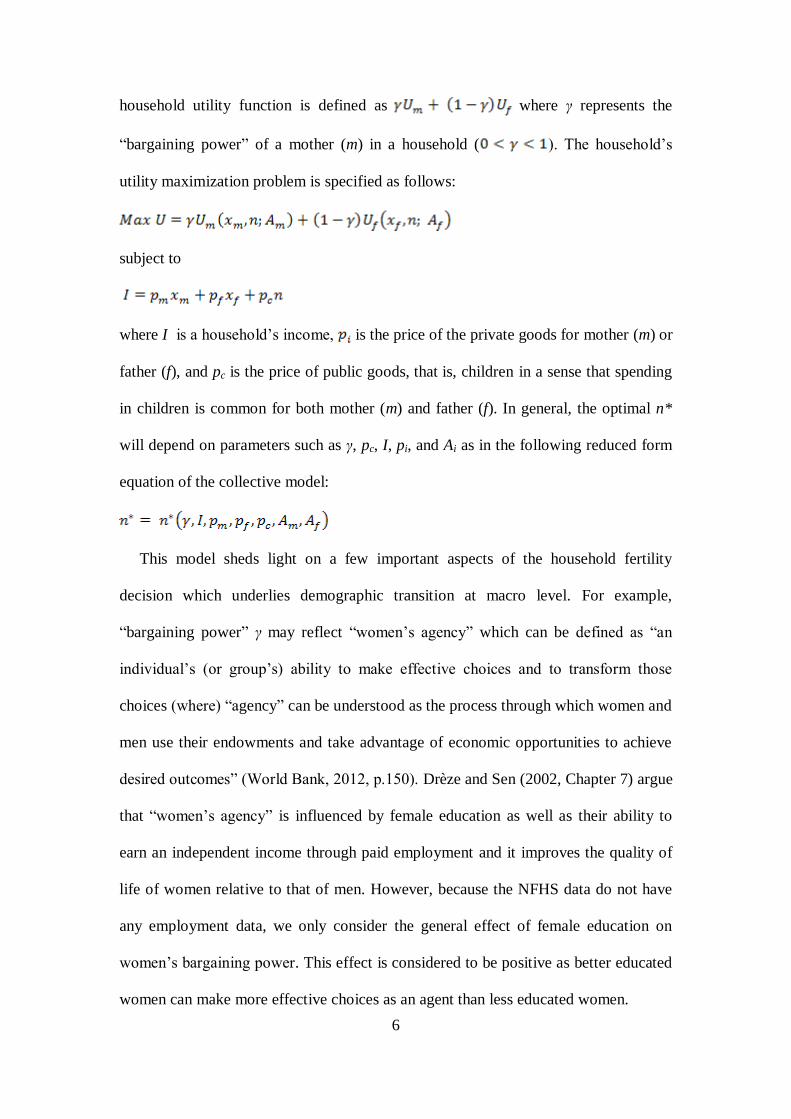
household utility function is defined as where γ represents the
“bargaining power” of a mother (m) in a household ( ). The household’s
utility maximization problem is specified as follows:
subject to
where I is a household’s income, is the price of the private goods for mother (m) or
father (f), and pc is the price of public goods, that is, children in a sense that spending
in children is common for both mother (m) and father (f). In general, the optimal n*
will depend on parameters such as γ, pc, I, pi, and Ai as in the following reduced form
equation of the collective model:
This model sheds light on a few important aspects of the household fertility
decision which underlies demographic transition at macro level. For example,
“bargaining power” γ may reflect “women’s agency” which can be defined as “an
individual’s (or group’s) ability to make effective choices and to transform those
choices (where) “agency” can be understood as the process through which women and
men use their endowments and take advantage of economic opportunities to achieve
desired outcomes” (World Bank, 2012, p.150). Drèze and Sen (2002, Chapter 7) argue
that “women’s agency” is influenced by female education as well as their ability to
earn an independent income through paid employment and it improves the quality of
life of women relative to that of men. However, because the NFHS data do not have
any employment data, we only consider the general effect of female education on
women’s bargaining power. This effect is considered to be positive as better educated
women can make more effective choices as an agent than less educated women.
7
It is further assumed here that the stronger bargaining power of mother (m) over
father (f) reflected in higher generally leads to fewer children, given that mother is
less likely than father, to value n, the number of children due to her health risk for
child bearing and/or her heavier load of household tasks imposed on her in raising
children in the future. A higher relative bargaining power of women over men may
thus lead women to have a larger influence on family planning.5 In this framework, a
higher level of female education is likely to reduce the number of children through the
higher bargaining power of mother, γ. That is, education will increase women’s
bargaining power, γ (or women’s agency), which in turn will reduce n*, the optimal
number of children.6
Furthermore, the preferences Ai represent each household member’s attitude
toward the fertility decision, which may be different in various classes, social groups,
religious communities, and regions, and they may move toward “small family value”
with social and economic changes.7 Economic growth increases a household’s income
level I with a consequent effect on consumption xi, and the number of children n*.
Implicit in the model is that an increase in the income level lowers n and increases xi.8
In addition, as women attend schools and participate in labour markets more than
they did previously and as the wages increase, the opportunity cost of raising children
pc will increase. As a consequence of the substitution effect, a household may reduce
its n*. This also predicts the negative relation between female education and the
number of children, which will be tested in subsequent sections.
In sum, the above simplified version of the collective household model implies that
(i) the higher bargaining power of mother (m), γ, decreases n*, an optimal number of
children; (ii) education of mother decreases n* through the increased bargaining power
of mother, γ (as an implication derived by (i)); (iii) a household’s income level I
8
decreases n*; (iv) the preferences Ai (e.g. social groups, religious communities, and
regions) influence n*; and (v) the higher pc (e.g. through a higher opportunity cost of
raising children due to higher female wages) reduces n*, an optimal number of
children. That is, social, household and individual characteristics will influence the
household decision between mother and father regarding the optimal number of
children a mother a woman will bear. We cannot test all the predictions or
implications of the model due to data constraints, but we will highlight some of these
in the subsequent sections.
3. Data
This study draws upon NFHS Data in 1992-3, 1998-9 and 2005-6 (or NFHS-1,
NFHS-2 and NFHS-3). The NFHS is a major nationwide, large multi-round survey
conducted in a representative sample of households in India with focus on health and
nutrition of household members, especially of women and young children.9 The
survey also contains the detailed data on fertility and mortality. A direct proxy for the
fertility rate is available from NFHS, which has a question to ask mothers aged 15- 49
years old on how many children they have borne, after excluding any miscarriage but
including any death of children. We used the number of children based on this
question as a dependent variable.
Table 2 summarizes the recent trend of total fertility rate (TFR)10
by region in
India. Overall, TFR declined from 1992 to 2005 across different areas and regions in
India. However, there remains a significant disparity between rural and urban areas.
Also noted is a disparity among different regions, reflecting disparity among different
states. TFRs are much lower in South (Andhra Pradesh, Karnataka, Kerala and Tamil
Nadu) and West (Goa, Gujarat and Maharashtra) than in Central (Madhya Pradesh

9
and Uttar Pradesh), East (Bihar, Orissa and West Bengal) or Northeast (Arunachal
Pradesh, Assam, Manipur, Meghalaya, Mizoram, Nagaland, Sikkim and Tripura).
North is roughly at the national average, while TFR is varied within North raging
from 1.94 in Himachal Pradesh and 1.99 in Punjab to 3.21 in Rajasthan in 2005.
(Table 2 to be inserted)
4. Econometric Models
The main objective of our econometric models is to identify the key determinants of
fertility proxied by the number of children. The basic idea of specifying the
econometric model of fertility behavior draws upon Drèze and Sen (2001).
(1) OLS Model
Using the cross sectional household data constructed by three rounds of NFHS, we
estimate the reduced form equation by OLS as a baseline model.11
DRSLMOBAEEnniiiii
m
i
f
i
m
iii,,,,,,,,, (1)
12
i denotes household and the dependent variable is i
n the number of children a mother
has borne. i
n is estimated by the following explanatory variables.
m
iE : A vector of the mother’s education (Case (A): whether literate or not; Case (B): a
set of dummy variables on the level of educational achievement of mother). In Case
(A), education is simply defined in terms of literacy of a mother, with focus on the
effect of being illiterate on fertility. In Case (B), we used a set of dummies, namely,
(i) whether attended or completed primary school, (ii) whether completed secondary
school, and (iii) whether completed higher education. Each dummy variable takes
either 1 or 0.
10
In general, female education can be considered to be a proxy for the opportunity
cost of raising children. The forgone income by, for example, leaving a job or shifting
from a full-time to a part-time job for childcare after giving birth may be larger for the
women who are more educated and tend to have the job with higher income.
Furthermore, an increase in female education will empower women and their
increased bargaining capability in households would enable them to control over the
fertility in India (Drèze and Murthi, 2001). Using the NFHS-2 and 3 data on Andhra
Pradesh, Sujatha and Reddy (2009) have shown that women’s autonomy in decision
making, access to money and freedom of movement increase with education and
reduces fertility. Moreover, educated women may be able to understand ‘the quality’
of children better and thus they may place more importance on ‘quality’ over
‘quantity’, which would reduce their desired number of children.
It is often argued that educated women also tend to have more knowledge of
contraception than illiterate women which will lead to the smaller number of children,
but the effect of education has to be understood in the context of family planning
programmes. When a central or state government provides the family planning
services to women, they tend to be availed only by educated women who are open-
minded and can understand the logic of family planning, and less educated women
groups generally large in size remain untouched (Singh, 2001). This would make the
negative relation between education and fertility even further pronounced.
Higher education also makes women delay the age of marriage or of giving birth to
the first child. This results in the negative relationship between women’s education
and the number of children particularly in case of OLS where the women in all the
age groups (15-49 years old) are pooled.13
Educated women with higher income

11
would place more importance on ‘quality’ of children over ‘quantity’ and this would
make the fertility-education correlation further negative.
f
iE : A vector of the father’s education (defined same as above).
Higher level of the father’s education might lead him to cooperate with mother in
developing the family plan and using contraceptives. This has been relatively
neglected in the literature with a few exceptions, such as, Bhat (2002). However,
because in many households men tend to spend much less time for childcare than
women, the negative link between education and fertility is expected to be weaker.
However, educated men who tend to be open-minded would be willing to listen to
women’s needs (e.g. preference for children’s ‘quality’) and to cooperate with women
for family planning. An expected sign of the coefficient estimate is thus negative.
m
iA : Mother’s age and its square, which take account of the life cycle effect of mother.
iB : Social backwardness of the household in terms of (i) whether a household
belongs to Scheduled Caste and (ii) whether it belongs to scheduled tribe.
iO : Occupation of parents in terms of (i) whether the household is classified as non-
agricultural self-employment and (ii) whether as agricultural self-employment. We
assume that self-employment households have a greater demand for child labour and
thus higher fertility. This is a permanent occupation category and not affected by
unemployment.
iM : Religion of the household. We use the Muslim dummy only in consideration of
the unique fertility behavior among Muslims. Fertility rates are supposed to be high
among Muslims because of their pronatalist ideology and opposition to family
planning or early marriages (e.g. Mouhasha and Rama Rao, 1999, Mishra, 2004, Bhat
and Zavier, 2005).
12
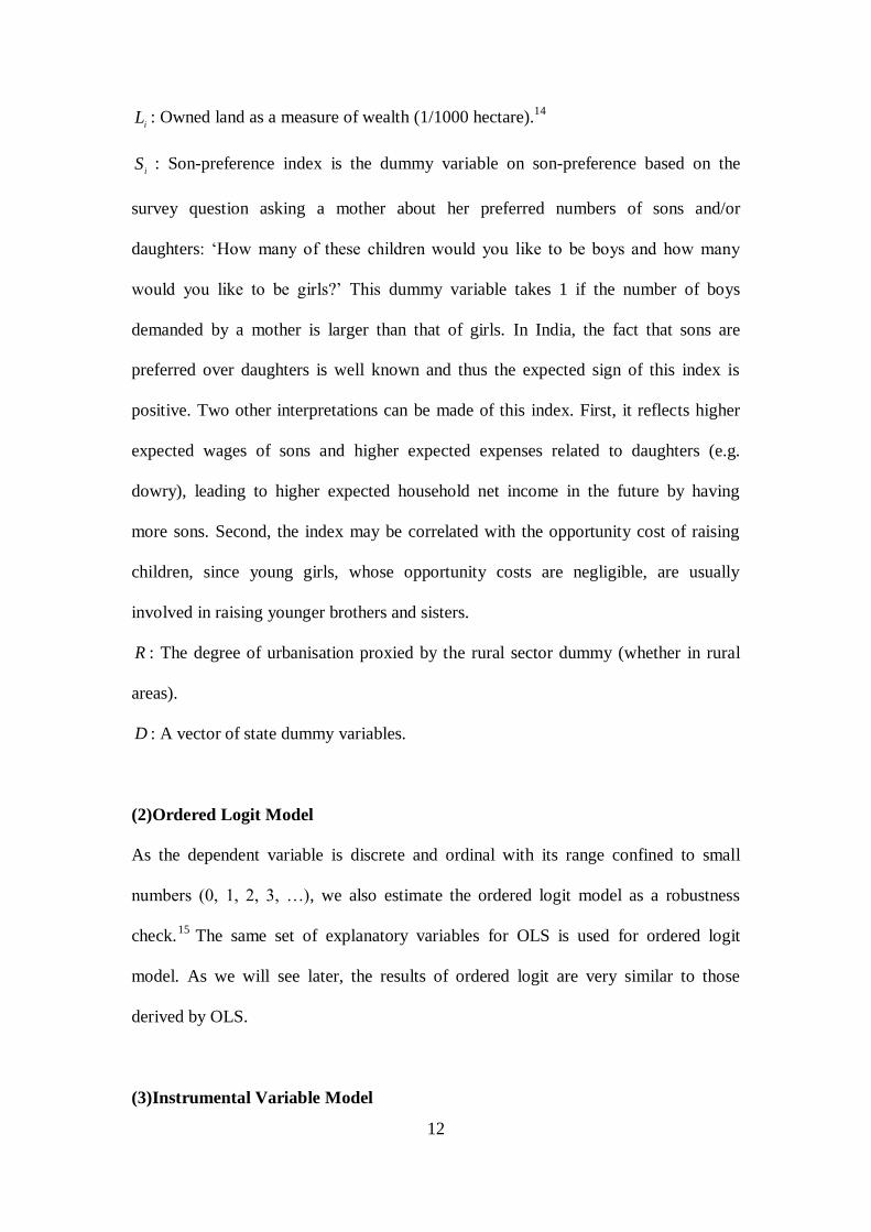
iL : Owned land as a measure of wealth (1/1000 hectare).
14
iS : Son-preference index is the dummy variable on son-preference based on the
survey question asking a mother about her preferred numbers of sons and/or
daughters: ‘How many of these children would you like to be boys and how many
would you like to be girls?’ This dummy variable takes 1 if the number of boys
demanded by a mother is larger than that of girls. In India, the fact that sons are
preferred over daughters is well known and thus the expected sign of this index is
positive. Two other interpretations can be made of this index. First, it reflects higher
expected wages of sons and higher expected expenses related to daughters (e.g.
dowry), leading to higher expected household net income in the future by having
more sons. Second, the index may be correlated with the opportunity cost of raising
children, since young girls, whose opportunity costs are negligible, are usually
involved in raising younger brothers and sisters.
R : The degree of urbanisation proxied by the rural sector dummy (whether in rural
areas).
D : A vector of state dummy variables.
(2) Ordered Logit Model
As the dependent variable is discrete and ordinal with its range confined to small
numbers (0, 1, 2, 3, …), we also estimate the ordered logit model as a robustness
check.15
The same set of explanatory variables for OLS is used for ordered logit
model. As we will see later, the results of ordered logit are very similar to those
derived by OLS.
(3) Instrumental Variable Model

13
For most of parents in India, the period for fertility starts after education is completed.
However, some young women give birth when they are in their late teens and for
them the decision on whether they should take secondary/higher education or marry
and give birth may be made simultaneously where ‘fertility’ may affect ‘female
education’ (i.e. the opposite direction of causality). Though the proportion of those
women is not likely to be so large16
, this may cause the correlation of education and
the error term, which will bias the coefficient estimate. Instrumental Variable (IV)
model, such as 2SLS, would partially address this issue. As a robustness check for
OLS, we estimate the IV model (Case (C)) where mother’s literacy is instrumented.
The IV model requires a valid instrument satisfying an exclusion restriction where the
instrument which affects the endogenous variable (mother’s literacy) does not have an
independent causal effect on the outcome (fertility).
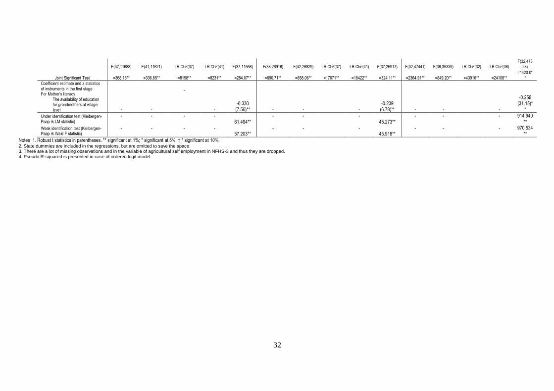
Finding such an instrument would be extremely difficult as the NFHS data do not
cover or allow us to construct such a variable due to the inherent data constraints. In
the present study, we use as an instrument the ratio of women who attended secondary
school in the total in the age group 50 or above averaged at the village level. This is a
proxy for general education levels or the availability of secondary education for
grandmothers, which would affect mother’s education, but not fertility directly
because the village-level aggregation has at least partially eliminated the direct link
between the fertility and the instrument. However, the validity of this instrument may
be questioned for various conceptual grounds. For example, many women in India
marry men outside the village, or better education in the previous generation reflects
better information about child health and nutrition and preference for child quality
over quantity. Given that the instrument is not perfect, the results will have to be
interpreted with caution. However, we would argue that this instrument is one of the

14
best ones due to the data constraints and it is justified as the specification passes
various statistical tests for the validity of instruments (e.g. under-identification and
weak identification tests presented at the bottom of Table 3). For pseudo panel data
model we discuss below, we have included only the women aged from 19 to 33 years
in the first round and thus the endogeneity issue is likely to be less relevant.
(4) Pseudo Panel Data Model
One of the limitations of the above model is that each round of NFHS is used
separately for the cross-sectional estimations. To overcome this and to identify the
determinants of fertility which are specific to a particular generation and common
over the years, we apply the pseudo panel model which aggregates micro-level
household data by any meaningful unit or cohort (e.g. geographical areas or age
groups) that is common across cross-sectional data sets in different years. We apply
the pseudo panel for the cohort k based on the combination of states and rural-urban
classifications. The cohort is denoted as k in the equation (2) below.
ktiktiktiktiktikt
m
ikt
m
iktiktiSLMOBAEnn ,,,,,, (2)
where k denotes cohort (i.e., age cohort state rural-urban classification) and t
stands for survey years for three rounds of NFHS, 1992, 1998 and 2005. The upper
bar means that the average of each variable is taken for each cohort, k for each round,
t . As mother’s education is highly correlated with father’s at the aggregate level, we
insert either kt
m
tE or
kt
f
tE at one time.
The equation (2) can be estimated by the standard static panel model, such as fixed
effects or random effects model.
kt
q
l kttkt
l
i
l
ktieDxn 1 (3)
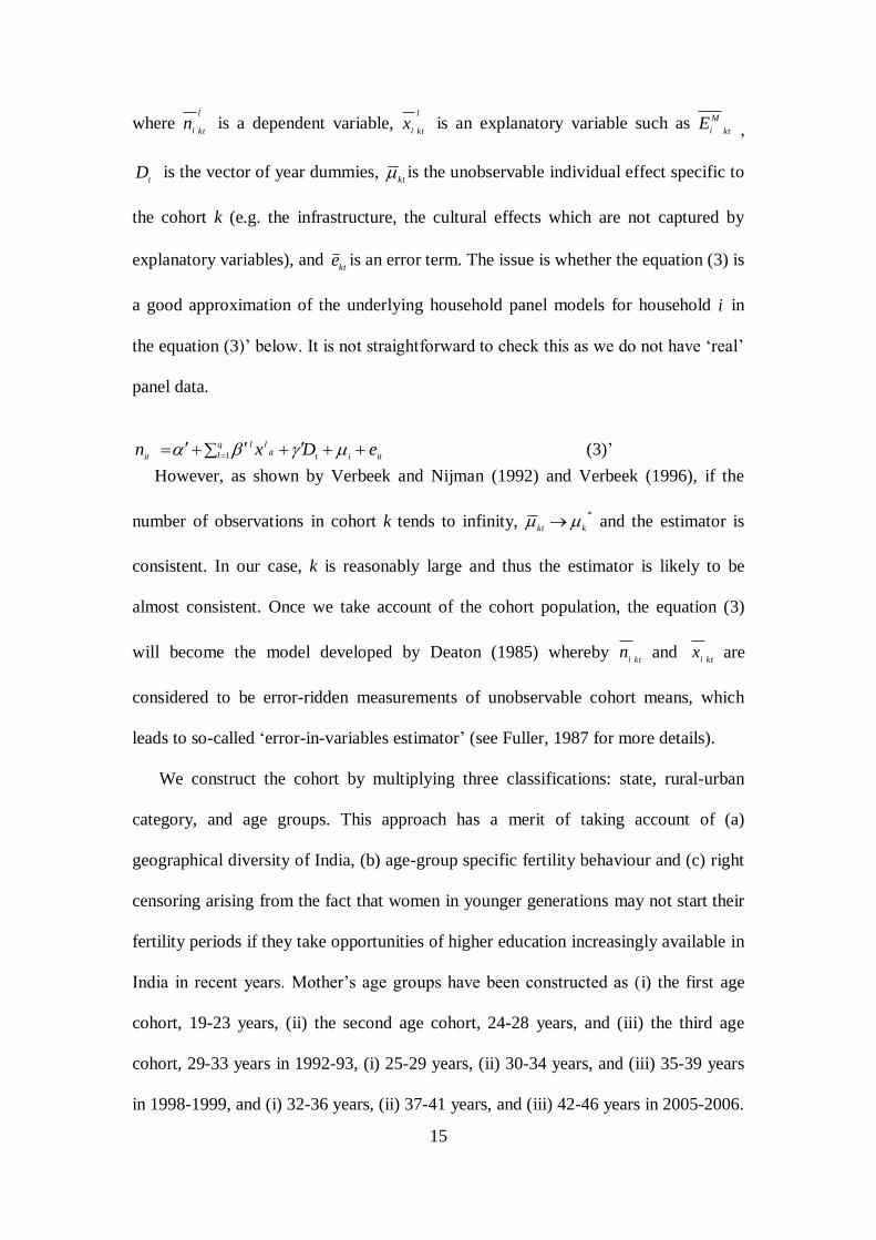
15
where l
ktin is a dependent variable,
l
ktix is an explanatory variable such as
kt
M
iE ,
tD is the vector of year dummies,
kt is the unobservable individual effect specific to
the cohort k (e.g. the infrastructure, the cultural effects which are not captured by
explanatory variables), and kt
e is an error term. The issue is whether the equation (3) is
a good approximation of the underlying household panel models for household i in
the equation (3)’ below. It is not straightforward to check this as we do not have ‘real’
panel data.
q
l itititll
iteDxn 1 (3)’
However, as shown by Verbeek and Nijman (1992) and Verbeek (1996), if the
number of observations in cohort k tends to infinity, *
kkt and the estimator is
consistent. In our case, k is reasonably large and thus the estimator is likely to be
almost consistent. Once we take account of the cohort population, the equation (3)
will become the model developed by Deaton (1985) whereby kti
n and kti
x are
considered to be error-ridden measurements of unobservable cohort means, which
leads to so-called ‘error-in-variables estimator’ (see Fuller, 1987 for more details).
We construct the cohort by multiplying three classifications: state, rural-urban
category, and age groups. This approach has a merit of taking account of (a)
geographical diversity of India, (b) age-group specific fertility behaviour and (c) right
censoring arising from the fact that women in younger generations may not start their
fertility periods if they take opportunities of higher education increasingly available in
India in recent years. Mother’s age groups have been constructed as (i) the first age
cohort, 19-23 years, (ii) the second age cohort, 24-28 years, and (iii) the third age
cohort, 29-33 years in 1992-93, (i) 25-29 years, (ii) 30-34 years, and (iii) 35-39 years
in 1998-1999, and (i) 32-36 years, (ii) 37-41 years, and (iii) 42-46 years in 2005-2006.

16
5. Main Results
In this section we will report and discuss econometric results for the models described
in the previous section. The results of cross-sectional estimations for the first, second
and third rounds of NFHS are reported in Table 3, while those of pseudo panel data
model are shown in Table 4.
(1) OLS, Ordered Logit, and IV Results for Households across all India
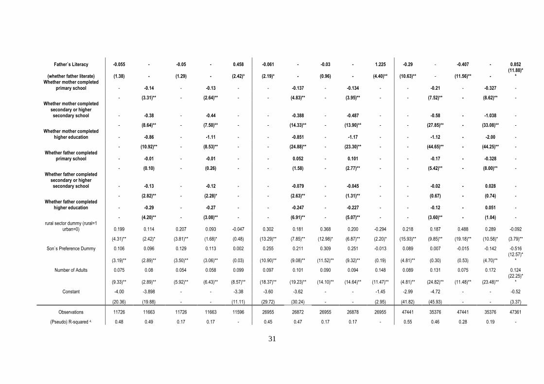
Table 3 presents five cases for three rounds of NFHS, – Case (A): OLS model with
literacy dummies for mother and father, Case (B): OLS model with a set of dummy
variables of their educational attainments, Case (C): ordered logit with literacy
dummies for mother and father, Case (D): ordered logit model with a set of dummy
variables of their educational attainments, and Cade (E): IV model where literacy
dummies are instrumented.17
(Table 3 to be inserted)
We first highlight the effects of education on fertility. In Case (A) (OLS) and Case
(C) (ordered logit), the dummy variable on mother’s literacy is all negative and
significant for all the three rounds – with the coefficient estimate increasingly
significant in the later rounds. The coefficient estimate of a mother’s literacy dummy
suggests that if a mother is literate, the number of children she has borne on average is
likely to be reduced by 0.303, 0.406, and 0.610 in 1992, 1998 and 2005 respectively,
ceteris paribus in Case (A) in which OLS is applied. The estimated reduction in the
number of children is larger in Case (C) (ordered logit) - 0.322, 0.490, and 1.01 in
1992, 1998 and 2005 respectively. These reductions seem substantial in comparison
with the average total fertility rate (TFR) as each figure of reduction corresponds to

17
9.6%, 14.2% and 22.8% of TFR in each year. It is also noted that the negative effect
of mother’s literacy on fertility is larger in more recent years in both Case (A) and
Case (C). It is not clear only from our regression results why mother’s literacy had an
increasingly negative effect on the number of children. It is surmised, however, that if
the average fertility of illiterate women has not changed dramatically, that of literate
women (some of whom became more likely to receive secondary or higher education
in later rounds) has been reduced over the years as a result of their increased
autonomy and bargaining power in the household.
Father’s literacy is negative and non-significant in 1992 and negative and
significant in 1998 and 2005 with the coefficient estimate more significant in the last
round in Case (A) (OLS). It is negative and significant only in 2005 in Case (C)
(ordered logit). While the absolute values of coefficient estimates of father’s literacy
is much smaller than that of mother’s literacy, it changes from -0.055 in 1992, to -
0.061 in 1998 and -0.290 in 2005 in Case (A). Mother’s education is generally
deemed a more important determinant of fertility than father’s education because
women are still responsible for childcare in a majority of households in India and thus
the income forgone by giving up a job is likely to be larger for women than for men.
However, father’s literacy became increasingly important in the last round with its
effect nearly half of the effect of mother’s literacy in Case (A). The reason for this is
not clear, but this might be due to some change in the bargaining relation between a
husband and a wife in favour of the latter because it is likely that women became
more and more educated and empowered in the later rounds, which might change the
behavioral response of literate men who began to cooperate with family planning in
recent years.

18
The effects of dummy variables on educational attainment of mother and father
have been examined in Case (B) (OLS) and Case (D) (ordered logit). For all the three
levels (i.e. completed only primary school, only secondary or higher secondary school,
and higher education), mother’s education is negative and significant across all the
three rounds in both cases. The absolute values of coefficient estimates are similar in
1992 and in 1998, but it is substantially larger for all the levels in 2005. For example,
if a household has a mother completing only primary school, the number of children
reduces by 0.21 (or 0.327) in 2005 in Case (B) (or Case (D)), ceteris paribus. This
will increase to 0.58 (or 1.038) for completion of secondary or higher secondary
school and 1.12 (or 2.00) for higher education in Case (B) (or Case (D)). This
confirms the increasing role of mother’s education as we have discussed above. On
the role of father’s education, the coefficient estimates of educational attainments are
negative and significant except for primary education in the first two rounds and
secondary or higher secondary school in the last round. While the results imply that
father’s education reduces the number of children, its marginal effects are much
smaller than mother’s education. Contrary to our expectation, the effect of father
competing higher education was getting smaller in absolute terms over the years with
the coefficient estimate changing from -0.290, -0.247 to -0.120 in Case (B) (or from -
0.270, -0.227 to 0.051 in Case (D)). The reason is again not clear, but it is noted that
the effect of father’s completing primary education in reducing fertility became
relative larger in the last round (-0.17) (the magnitude of which became closer to
mother’s completing primary education (-0.21)) in Case (B). That is, if men had basic
or primary education, they would become able to, for example, understand the logic
of family planning, or be willing to cooperate with women in the household

19
bargaining, while completing secondary or higher education has a relatively small
impact on fertility.
Case (E) reports the results of IV model. Given the limitation of our instrument,
the results will have to be interpreted with caution.18
Though the coefficient estimates
are less statistically significant, the pattern of the results for mother’s literacy in Case
(E) is similar to the corresponding results in Case (A) or Case (C). That is, the role of
mother’s literacy in reducing fertility has become more and more important in the
later rounds. However, father’s literacy is positive and significant in Case (E) in all
the rounds. Since the reason is not clear and given the limitation of our instrument in
Case (E), we would use Cases (A) and (C) as our preferred cases for the following
discussion.19
Our results confirm the greater role of female education in fertility reduction as
emphasized by earlier studies, for example, Brookins and Brookins (2002), Drèze and
Sen (2002), Drèze and Murthi (2001), Subbarao and Raney (1985), and Jain and Nag
(1986). While Drèze and Murthi (2001) and Drèze and Sen (2002) claim that male
literacy makes no contribution to reduction in fertility when controlled by female
education, our study shows that both male literacy and education attainments are
closely associated with fertility reduction in both OLS and ordered logit.
Turning to the results of other variables, all the cases for three rounds show that the
coefficient estimate of mother’s age is positive and significant and its square is
negative and significant, which reflects the non-linearity in the age-fertility
relationship. The coefficient estimate of Scheduled Caste (SC) dummy is positive and
significant in both OLS and ordered logit, whilst that of scheduled tribe (ST) dummy
is positive and significant only in the last round in these cases. ST dummy is negative
and significant in Case (E) or IV across three rounds. The current results alone will
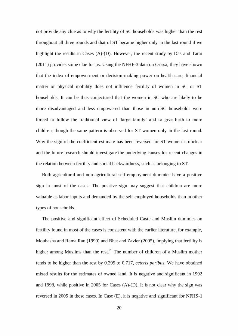
20
not provide any clue as to why the fertility of SC households was higher than the rest
throughout all three rounds and that of ST became higher only in the last round if we
highlight the results in Cases (A)-(D). However, the recent study by Das and Tarai
(2011) provides some clue for us. Using the NFHF-3 data on Orissa, they have shown
that the index of empowerment or decision-making power on health care, financial
matter or physical mobility does not influence fertility of women in SC or ST
households. It can be thus conjectured that the women in SC who are likely to be
more disadvantaged and less empowered than those in non-SC households were
forced to follow the traditional view of ‘large family’ and to give birth to more
children, though the same pattern is observed for ST women only in the last round.
Why the sign of the coefficient estimate has been reversed for ST women is unclear
and the future research should investigate the underlying causes for recent changes in
the relation between fertility and social backwardness, such as belonging to ST.
Both agricultural and non-agricultural self-employment dummies have a positive
sign in most of the cases. The positive sign may suggest that children are more
valuable as labor inputs and demanded by the self-employed households than in other
types of households.
The positive and significant effect of Scheduled Caste and Muslim dummies on
fertility found in most of the cases is consistent with the earlier literature, for example,
Mouhasha and Rama Rao (1999) and Bhat and Zavier (2005), implying that fertility is
higher among Muslims than the rest.20
The number of children of a Muslim mother
tends to be higher than the rest by 0.295 to 0.717, ceteris paribus. We have obtained
mixed results for the estimates of owned land. It is negative and significant in 1992
and 1998, while positive in 2005 for Cases (A)-(D). It is not clear why the sign was
reversed in 2005 in these cases. In Case (E), it is negative and significant for NFHS-1

21
and 3. The son preference dummy variable is mostly positive and significant in Cases
(A)-(D), but it is negative and significant in Case (E) (IV) for NFHS-3. Taking OLS
and ordered logit as our preferred cases, the positive coefficient estimate of son
preference dummy implies that mothers who prefer sons tend to have more children
and thus high fertility results. This is consistent with earlier studies, such as Drèze and
Sen (2002).
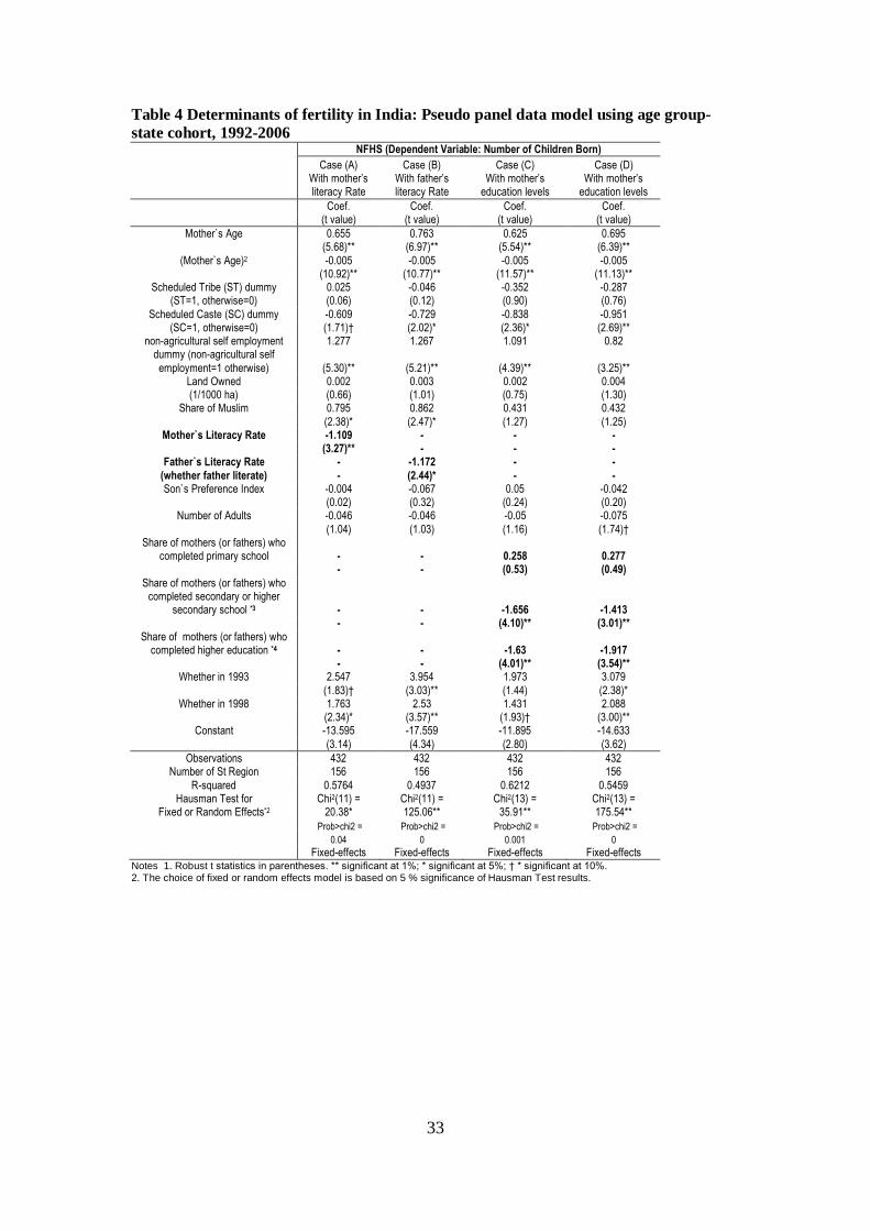
(2) Results of Pseudo Panel Model
Table 4 presents the results based on pseudo panel models based on cohorts
constructed by (a) age cohorts, (b) state, and (c) a rural and urban classification. A
few points are noted on the selection of explanatory variables. First, we use education
variables (literacy or a set of educational levels) separately for a father and a mother
as they are correlated at the aggregate level.21
Second, the results based on fixed-
effects model are presented following the results of Hausman tests which favour fixed
effects models over random-effects models in all cases. Four cases are shown
according to whether education is for mother or father and how education is defined,
i.e. the literacy rate or the educational attainments. Case (A) is the case with mother’s
literacy rate, Case (B) is with father’s literacy rate, Case (C) is the case with mother’s
educational attainments as shares, and Case (D) is with father’s educational
attainments. As we discussed, three age cohorts for mothers were traced for the entire
period of 14 years from 1992 to 2006. As a robustness check to take account of right
censoring, we have tried the cases only with the second and the third cohorts and
those only with the third cohort. To save the space, only the cases with all 3 cohorts
are presented in Table 4.
(Table 4 to be inserted)
22
The results in Table 4 are broadly consistent with those in Table 3. Table 4 shows
that coefficient estimates of variables on mother or father’s education are mostly
negative and significant regardless of the definition of education. It is noted that these
negative effects are observed with similar patterns in the cases with the second and
third age cohorts and those with the third age cohort only.22
Because pseudo panel
involves averaging a dependent variable and explanatory variables within a cohort,
there is little difference in the absolute values of coefficient estimates for mother’s
education and father’s education. These results are important as we have taken
account of (1) age-specific fertility behavior over the years, (2) time-series changes in
fertility rates at regional cohort, and (3) right censoring due to the fact that young
mothers may not start their fertility period if they participate in attend higher
education. Our results are consistent with the role of parental education in reducing
fertility rates in India.
On other variables, we obtain the coefficient estimates with same signs and
significance as obtained by household data for mother’s age (positive) and its square
(negative), and non-agricultural self-employed dummies (positive). Those of Schedule
Caste are negative and significant, which is consistent with the results of Table 3.
Share of Muslim is positive and significant in Case (A) and Case (B). Son’s
preference index is statistically insignificant. This is probably because there is little
inter-state variation in son’s preference index (that is, the extent to which mother
prefers son is not much different among different states) which resulted in
insignificant coefficient estimates in the case of pseudo panel model, while the intra-
state variation of the index has mainly driven the significant estimates in OLS in
Table 3.
23
6. Concluding Observations
This paper examines the determinants of fertility and its changes drawing upon three
rounds of NFHS data over the period 1992-2006. That fertility declined dramatically
in many parts of India during the period is consistent with the view that India is seen
to be moving through the second stage toward the third stage of demographic
transition. The investigation of fertility in India is important not only for providing an
insight into the population problem for the second populous country in the world. It
also serves as a background for the debate on poverty in India which would be
influenced by the geographical pattern of population growth. This paper sheds an
empirical light on the determinants of fertility by applying econometric models to the
large household data sets constructed by NFHS data. Our main findings are
summarized below.
Consistent with the literature, mother’s education is related to reduction in fertility.
We have confirmed a negative and significant association of the number of children
and mother’s education - defined in terms of both literacy and educational attainments.
More importantly, the role of mother’s education in reducing fertility became
increasingly important over the years. The negative link between mother’s education
and fertility has been reported in the past (e.g. Drèze and Murthi, 2001), but the past
studies used the district-level data or the data which aggregate the census data at
district levels in the context of India. The present study is the first, to our knowledge,
to show this link using the nation-wide household survey data. Our contribution to the
literature has also been made by tracing the data over the period spanning from 1992
to 2006 and by confirming that the negative association between mother’s education
and fertility has become stronger in recent years. Furthermore, we have found

24
significant and negative coefficient estimates for father’s education in case of OLS
and ordered logit. However, its effect is generally smaller than mother’s education.
Few studies have focused on the role of father’s education on fertility and this is also
a unique contribution of the present study.
The negative and significant effects of parental education have been observed
when we run the pseudo panel regressions for age cohorts further classified by state,
and rural-urban classification. The negative effect of education of parents is
unchanged regardless of the definition of education and of the age cohorts to be
included and it is consistent with the role of parental education in reducing fertility.
The findings based on OLS and ordered logit have been confirmed by pseudo panel
models by which age-group specific fertility behavior or time-series effects are taken
into account.
Our econometric results identify other factors, such as, social backwardness, land
owned or religion, which are important determinants of fertility. It is implied that the
women in Scheduled Castes (SCs) who are likely to be more disadvantaged and less
empowered than those belonging to non-SCs tend to have more children, while the
results on Scheduled Tribe (ST) are mixed where both positive and negative
coefficient estimates are found in different cases. We have also found that Muslim
households tend to have more children than the rest.
Our results suggest that policies of national and state governments to support social
infrastructure, such as school at various levels and to promote both male and female
education, would be very important to reduce fertility and to speed down the
population growth. These policies would play particularly important roles in
backward states or for socially disadvantaged groups (e.g. Scheduled Castes) which
have higher fertility as well as poverty rates.
25
References
Bardhan, P. & Udry, C. (1999) Development Microeconomics (New York: Oxford
University Press).
Basu, K. (2006) Gender and Say: a Model of Household Behaviour with
Endogenously Determined Balance of Power, The Economic Journal, 116, pp.
558-580.
Becker, G. S. (1960) An Economic Analysis of Fertility, in Demographic and
Economic Change in Developed Countries: a conference of the Universities-
National Bureau Committee for Economic Research. ed. George B. Roberts
(Chairman, Universities-National Bureau Committee for Economic Research)
(New York: Princeton University Press), pp.209-240.
Becker, G. S. (1981) A Treatise on the Family (Cambridge: Harvard University Press).
Becker, G. S. & Lewis, H. G. (1973) On the Interaction between Quantity and Quality
of Children, Journal of Political Economy, 81, pp.S279-S288.
Bhalotra, S. & van Soest, A. (2008) Birth-Spacing, Fertility and Neonatal Mortality in
India: Dynamics, Frailty, and Fecundity, Journal of Econometrics, 143, pp.274-
290.
Bhat, P. N. M., (2002) Returning a Favor: Reciprocity Between Female Education and
Fertility in India, World Development, 30(10), pp.1791–1803.
Bhat, P. N. M. & Zavier, A. J. F. (2005) Role of Religion in Fertility Decline,
Economic & Political Weekly, 40(5), pp.385-402, January 29.
Bose, A. (2000) North-South Divide in India's Demographic Scene, Economic and
Political Weekly, pp.1698-1699, May 13.
Brookins, M. L. & Brookins, O. T. (2002) An exploratory analysis of fertility
differentials in India, Journal of Development Studies, 39(2), pp.54-72.
26
Browning, M. & Chiappori, P. A. (1998) Efficient Intra-Household Allocations,
Econometrica, 66(6), pp.1241-1278.
Browning, M. & Gørtz, M. (2012) Spending Time and Money within the Household,
Scandinavian Journal of Economics, 114(3), pp. 681-704.
Das, B. & Tarai, D. (2011) Decision-making and Fertility Behaviour: A Comparative
Analysis of Scheduled Caste and Scheduled Tribe Women in Odisha, Social
Change, 41(2), pp.233–249.
Deaton, A. (1985) Panel Data from the Time Series of Cross-Sections, Journal of
Econometrics, 30, pp.109-126.
Drèze, J. & Sen, A. (2002) India: Development and Participation (New Delhi, Oxford
University Press).
Drèze, J. & Murthi, M. (2001) Fertility, Education and Development, Population and
Development Review, 27(1), pp.33-63.
Fuller, W. A. (1987) Measurement Error Models, Wiley and Sons, New York.
Greene, W. (2003) Econometric Analysis, Fifth Edition, Prentice Hall, New Jersey.
Himanshu (2007) Recent Trends in Poverty and Inequality: Some Preliminary
Results, Economic and Political Weekly 42, pp.497-508, February 10.
International Institute for Population Science (2001) National Family Health Survey:
India 1998-99 (Mumbai, IIPS).
Imai, K. & Sato, T. (2010) Fertility, Parental Education and Development in India:
Evidence from National Household Survey Data, RIEB Discussion Paper Series
DP2010-17 (Kobe: Kobe University).
Imai, K., Annim, S.K., Gaiha, R., and Kulkarni, V.S. (2012) Does Women’s
Empowerment Reduce Prevalence of Stunted and Underweight Children in Rural
India?, RIEB Discussion Paper Series DP2012-11 (Kobe: Kobe University).
27
Jain, A. & Nag, M. (1986) The Importance of Female Primary Education for Fertility
Reduction in India, Economic and Political Weekly, 21(36), pp.1602-1608,
September 6.
Mahbub ul Haq Human Development Center (2002) Human Development in South
Asia 2001 Globalisation and Human Development (Karachi, Oxford University
Press).
Mishra, V. (2004) ‘Muslim/Non-Muslim Differentials in Fertility and Family
Planning in India’, East-West Center Working Papers- Population Health Series
No. 122, Jan 2004.
Moulasha, K. & Rao, G. R. (1999) Religion-Specific Differentials in Fertility and
Family Planning, Economic and Political Weekly, 34(42-43), pp.3047-51, October
16-23.
Vallely, P. (2008) Population paradox: Europe's time bomb, The article in the
Independent, August 9, 2008,
http://www.independent.co.uk/news/world/europe/population-paradox-europes-
time-bomb-888030.html.
Rosenzweig, M. (1990) Population growth and human capital investments: theory and
evidence, Journal of Political Economy, 98(5), pp.S12- S70.
Singh, A. (2001) ‘Education, Fertility and Fertility Preferences’, on-line article,
http://news.wikinut.com/Education,-Fertility-and-Fertility-Preferences/rwgg_59f/
(accessed on 30th September 2011).
Subbarao, K. & Raney, L. (1995) Social Gains from Female Education, Economic
Development and Cultural Change, 44, pp.105-28.
Sujatha, D. S. & Reddy, G. B. (2009) Women’s Education, Autonomy and Fertility
Behaviour, Asia-Pacific Journal of Social Sciences, 1(1), pp.35-50.
28
United Nations (2012) World Population Prospects: The 2011 Revision (New York,
Population Division of the Department of Economic and Social Affairs of the
United Nations Secretariat).
Verbeek, M. (1996) Pseudo Panel Data in Matyas, L. & Sevestre, P. (Eds.), The
econometrics of panel data: A handbook of the theory with applications, second
edition, in Advanced Studies in Theoretical and Applied Econometrics, vol. 33.
(Boston and London, Kluwer Academic), pp. 280-92.
Verbeek, M. & Nijman T. E. (1992) Can Cohort Data Be Treated As Genuine Panel
Data? Empirical Economics 17, pp.9-23.
World Bank (2012) World Development Report 2012: Gender Equality and
Development (New York, Oxford University Press).

29
Table 1 Population Projection for India, China, Sub-Saharan Africa and World in 2005
India China SSA*2.
World
1980 700 983 375 4453
(15.7%) (22.1%) (8.4%) (100%)
2010 1225 1341 823 6896
(17.8%) (19.4%) (11.9%) (100%)
2050 1692 1296 1892 9306
(18.2%) (13.9%) (20.3%) (100%)
*1. Unit: million. The number in the brackets: share in the world.
*2. Sub-Saharan Countries total.
*3. Source: UN (2012). The figures in 2050 are the estimate of medium variant.
Table 2 Total Fertility Rate for 15-49 in India based on NFHS-1, 2 and 3 (1992-3, 1998-9
and 2005-6) URBAN RURAL Total
1992 1998 2005 1992 1998 2005 1992 1998 2005
North 2.69 2.15 1.95 3.60 2.98 2.68 3.32 2.71 2.43
Central 3.43 2.75 2.66 4.65 3.94 3.64 4.36 3.65 3.37
East 2.64 2.21 2.04 3.46 2.86 3.04 3.28 2.75 2.82
Northeast 2.53 2.08 2.09 2.70 3.43 3.17 3.31 3.12 2.87
West 2.33 2.09 1.87 2.76 2.53 2.31 2.58 2.34 2.11
South 2.22 1.90 1.76 2.60 2.22 1.99 2.48 2.13 1.90
All India 2.70 2.27 2.06 3.67 3.07 2.98 3.39 2.85 2.68
Source: Based on National Familiy Health Survey in 1998-99 and 2005-6 (Table 4.3)

30
Table 3 Determinants of fertility in India (OLS, Ordered Logit Model and IV Model for cross-sectional household data) NFHS-1 (1992/3) NFHS-2 (1998/9) NFHS-3 (2005/6)
Case (A) Case (B) Case (C) Case (D) Case (E) Case (A) Case (B) Case (C) Case (D) Case (E) Case (A) Case (B) Case (C) Case (D) Case (E)
OLS
OLS Ordered
Logit Ordered
Logit IV
OLS
OLS Ordered
Logit Ordered
Logit
IV OLS OLS Ordered
Logit Ordered
Logit IV
Coef. Coef. Coef. Coef. Coef. Coef. Coef. Coef. Coef. Coef. Coef. Coef. Coef. Coef. Coef.
Explanatory Variables (t value) (t value) (t value) (t value) (t value) (t value) (t value) (t value) (t value) (t value) (t value) (t value) (t value) (t value) (t value)
Mother`s Age 0.221 0.23 0.41 0.42 0.240 0.211 0.222 0.41 0.43 0.188 0.185 0.261 0.686 0.543 0.096
(18.26)** (18.82)** (27.58)** (28.21)** (16.57)** (28.70)** (30.36)** (40.59)** (42.62)** (16.35)** (50.46)** (47.70)** (75.32)** (53.83)**
(14.91)*
*
(Mother`s Age)2 -0.001 -0.086 -0.004 -0.004 -0.002 -0.001 -0.001 -0.004 -0.004 -0.001 -0.001 -0.003 -0.007 -0.005 0.0001
(6.05)** (6.78)** (16.51)** (17.30)** (6.30)** (11.12)** (12.82)** (24.59)** (26.68)** (7.61)** (20.44)** (27.04)** (55.68)** (36.06)** (1.29)
Scheduled Tribe (ST) dummy (ST=1, otherwise=0) -0.082 -0.086 -0.040 -0.004 -0.293 0.048 0.016 0.048 0.001 -0.434 0.124 0.249 0.207 -0.360 -0.081
(1.48) (1.56) (0.66) (0.71) (3.13)** (1.27) (0.44) (1.10) (0.03) (3.77)** (4.78)** (7.09)** (4.76)** (7.85)** (2.34)**
Scheduled Caste (SC) dummy (SC=1, otherwise=0) 0.267 0.242 0.250 0.230 0.070 0.273 0.206 0.309 0.222 -0.252 0.181 0.234 0.380 0.384 -0.033
(4.75)** (4.31)** (4.12)** (3.77)** (0.77) (10.04)** (7.55)** (9.67)** (6.92)** (2.11)* (9.78)** (9.33)** (11.33)** (10.79)** (1.26)
non-agricultural self employment dummy (non-agricultural self
employment=1 otherwise) 0.194 0.071 0.215 0.074 -0.032 0.016 0.006 0.019 0.007 0.150 0.035 0.04 0.369 0.017 0.186
(4.35)** (1.49) (3.98)** (1.29) (0.35) (0.67) (0.24) (0.62) (0.21) (3.44)** (2.20)** (2.48)* (14.49)** (0.66) (8.98)**
agricultural self employment
dummy (agricultural self employment=1 otherwise=0) *3 0.209 0.068 0.233 0.076 -0.152 0.069 0.009 0.010 0.025 -0.217 - - - - -
(4.56)** (1.38) (4.36)** (1.33) (1.12) (2.88)** (0.39) (3.53)** (0.86) (3.06)** - - - - -
Land Owned (1/1000 ha) -0.001 -0.000 -0.002 -0.002 -0.0007 -0.004 -0.004 -0.006 -0.005 -0.005 0.006 0.015 0.026 0.045 0.002
(3.40)** (3.05)* (3.51)* (3.24)** (1.88)† (1.89)† (1.80)† (2.37)* (2.21)* (2.13)* (5.51)** (7.85)** (13.76)** (16.71)** (1.71)†
Muslim dummy(Muslim=1, otherwise=0) 0.325 0.295 0.338 0.301 0.210 0.509 0.404 0.603 0.467 0.050 0.382 0.54 0.801 0.879 0.116
(4.39)** (3.96)** (4.54)** (4.00)** (2.40)* (13.31)** (10.54)** (14.15)** (10.84)** (0.45) (16.34)** (16.49)** (20.05)** (20.36)** (3.58)**
Mother`s Literacy -0.303 - -0.322 - -1.983 -0.406 - -0.49 - -3.868 -0.61 - -1.01 - -3.033
(whether mother literate) (8.25)** - (7.39)** - (3.36)** (17.29)** - (17.55)** - (5.19)** (35.36)** - (42.25)** - (22.96)*
*
31
Father`s Literacy -0.055 - -0.05 - 0.458 -0.061 - -0.03 - 1.225 -0.29 - -0.407 - 0.852
(whether father literate) (1.38) - (1.29) - (2.42)* (2.19)* - (0.96) - (4.40)** (10.63)** - (11.56)** - (11.88)*
* Whether mother completed
primary school - -0.14 - -0.13 - - -0.137 - -0.134 - - -0.21 - -0.327 -
- (3.31)** - (2.64)** - - (4.83)** - (3.95)** - - (7.52)** - (8.62)** -
Whether mother completed
secondary or higher secondary school - -0.38 - -0.44 - - -0.388 - -0.487 - - -0.58 - -1.038 -
- (8.64)** - (7.50)** - - (14.33)** - (13.90)** - - (27.85)** - (33.08)** -
Whether mother completed higher education - -0.86 - -1.11 - - -0.851 - -1.17 - - -1.12 - -2.00 -
- (10.92)** - (8.53)** - - (24.88)** - (23.30)** - - (44.65)** - (44.25)** -
Whether father completed primary school - -0.01 - -0.01 - - 0.052 - 0.101 - - -0.17 - -0.328 -
- (0.10) - (0.26) - - (1.58) - (2.77)** - - (5.42)** - (8.00)** -
Whether father completed secondary or higher secondary school - -0.13 - -0.12 - - -0.079 - -0.045 - - -0.02 - 0.028 -
- (2.82)** - (2.28)* - - (2.63)** - (1.31)** - - (0.67) - (0.74) -
Whether father completed higher education - -0.29 - -0.27 - - -0.247 - -0.227 - - -0.12 - 0.051 -
- (4.20)** - (3.08)** - - (6.91)** - (5.07)** - - (3.60)** - (1.04) -
rural sector dummy (rural=1 urban=0) 0.199 0.114 0.207 0.093 -0.047 0.302 0.181 0.368 0.200 -0.294 0.218 0.187 0.488 0.289 -0.092
(4.31)** (2.42)* (3.81)** (1.68)* (0.48) (13.29)** (7.85)** (12.98)* (6.87)** (2.20)* (15.93)** (9.85)** (19.18)** (10.58)* (3.79)**
Son`s Preference Dummy 0.106 0.096 0.129 0.113 0.002 0.255 0.211 0.309 0.251 -0.013 0.089 0.007 -0.015 -0.142 -0.516
(3.19)** (2.89)** (3.50)** (3.06)** (0.03) (10.90)** (9.08)** (11.52)** (9.32)** (0.19) (4.81)** (0.30) (0.53) (4.70)**
(12.57)*
*
Number of Adults 0.075 0.08 0.054 0.058 0.099 0.097 0.101 0.090 0.094 0.148 0.089 0.131 0.075 0.172 0.124
(9.33)** (2.89)** (5.92)** (6.43)** (8.57)** (18.37)** (19.23)** (14.10)** (14.64)** (11.47)** (4.81)** (24.82)** (11.48)** (23.48)**
(22.25)*
*
Constant -4.00 -3.898 - - -3.38 -3.60 -3.62 - - -1.45 -2.99 -4.72 - - -0.52
(20.36) (19.88) - - (11.11) (29.72) (30.24) - - (2.95) (41.82) (45.93) - - (3.37)
Observations 11726 11663 11726 11663 11596 26955 26872 26955 26878 26955 47441 35376 47441 35376 47361
(Pseudo) R-squared 4. 0.48 0.49 0.17 0.17 - 0.45 0.47 0.17 0.17 - 0.55 0.46 0.28 0.19 -
32
Joint Significant Test
F(37,11688) F(41,11621) LR Chi2(37) LR Chi2(41) F(37,11558) F(38,26916) F(42,26829) LR Chi2(37) LR Chi2(41) F(37,26917) F(32,47441) F(36,35339) LR Chi2(32) LR Chi2(36) F(32,473
28)
=368.15** =336.65** =8158** =8231** =284.07** =690.71** =658.06** =17671** =18422** =324.11** =2364.91** =849.20** =43916** =24108** =1420.0*
*
Coefficient estimate and z statistics of instruments in the first stage For Mother’s literacy
The availability of education for grandmothers at village level - -
-
- -0.330
(7.56)** - -
- -0.239
(6.78)** - -
-
-0.256 (31.15)*
*
Under identification test (Kleibergen-Paap rk LM statistic)
-
-
- -
61.494**
-
-
-
45.273**
-
-
-
914.940
**
Weak identification test (Kleibergen-Paap rk Wald F statistic)
-
-
- - 57.203**
-
-
- 45.918**
-
-
-
970.534**
Notes 1. Robust t statistics in parentheses. ** significant at 1%; * significant at 5%; † * significant at 10%. 2. State dummies are included in the regressions, but are omitted to save the space. 3. There are a lot of missing observations and in the variable of agricultural self employment in NFHS-3 and thus they are dropped. 4. Pseudo R-squared is presented in case of ordered logit model.
33
Table 4 Determinants of fertility in India: Pseudo panel data model using age group-
state cohort, 1992-2006 NFHS (Dependent Variable: Number of Children Born)
Case (A) Case (B) Case (C) Case (D)
With mother’s literacy Rate
With father’s literacy Rate
With mother’s education levels
With mother’s education levels
Coef. (t value)
Coef. (t value)
Coef. (t value)
Coef. (t value)
Mother`s Age 0.655 0.763 0.625 0.695 (5.68)** (6.97)** (5.54)** (6.39)**
(Mother`s Age)2 -0.005 -0.005 -0.005 -0.005 (10.92)** (10.77)** (11.57)** (11.13)**
Scheduled Tribe (ST) dummy 0.025 -0.046 -0.352 -0.287 (ST=1, otherwise=0) (0.06) (0.12) (0.90) (0.76)
Scheduled Caste (SC) dummy -0.609 -0.729 -0.838 -0.951 (SC=1, otherwise=0) (1.71)† (2.02)* (2.36)* (2.69)**
non-agricultural self employment 1.277 1.267 1.091 0.82 dummy (non-agricultural self
employment=1 otherwise) (5.30)** (5.21)** (4.39)** (3.25)** Land Owned 0.002 0.003 0.002 0.004 (1/1000 ha) (0.66) (1.01) (0.75) (1.30)
Share of Muslim 0.795 0.862 0.431 0.432
(2.38)* (2.47)* (1.27) (1.25) Mother`s Literacy Rate -1.109 - - -
(3.27)** - - - Father`s Literacy Rate - -1.172 - -
(whether father literate) - (2.44)* - - Son`s Preference Index -0.004 -0.067 0.05 -0.042
(0.02) (0.32) (0.24) (0.20) Number of Adults -0.046 -0.046 -0.05 -0.075
(1.04) (1.03) (1.16) (1.74)† Share of mothers (or fathers) who
completed primary school - - 0.258 0.277 - - (0.53) (0.49)
Share of mothers (or fathers) who completed secondary or higher
secondary school *3 - - -1.656 -1.413 - - (4.10)** (3.01)**
Share of mothers (or fathers) who completed higher education *4 - - -1.63 -1.917
- - (4.01)** (3.54)** Whether in 1993 2.547 3.954 1.973 3.079
(1.83)† (3.03)** (1.44) (2.38)* Whether in 1998 1.763 2.53 1.431 2.088
(2.34)* (3.57)** (1.93)† (3.00)** Constant -13.595 -17.559 -11.895 -14.633
(3.14) (4.34) (2.80) (3.62)
Observations 432 432 432 432 Number of St Region 156 156 156 156
R-squared 0.5764 0.4937 0.6212 0.5459 Hausman Test for Chi2(11) = Chi2(11) = Chi2(13) = Chi2(13) =
Fixed or Random Effects*2 20.38* 125.06** 35.91** 175.54** Prob>chi2 = Prob>chi2 = Prob>chi2 = Prob>chi2 =
0.04 0 0.001 0
Fixed-effects Fixed-effects Fixed-effects Fixed-effects Notes 1. Robust t statistics in parentheses. ** significant at 1%; * significant at 5%; † * significant at 10%. 2. The choice of fixed or random effects model is based on 5 % significance of Hausman Test results.

34
Notes
1 See Vallely (2008) for the debate on this issue.
2 Poverty head count ratio based on the national poverty line in 2004/5 is 28.7% (Himanshu, 2007).
3 The theory of demographic transition explains the common pattern of transition in
population history. While the first stage of transition before economic modernisation sees
stable population due to high birth and death rates, the population grows rapidly in the second stage where death rates decline more rapidly than birth rates, for example, through
better educational systems and medical and health care facilities only available in
modernised society. The population becomes stable again in the third stage when further modernisation and better education cause fertility to go down.
4 For example, the average annual growth rate of GDP per capita of India in 1992-2006 is
4.7%, while the primary and secondary school enrolment increased from 70.1% in 1992 to 90.2% in 2006 (calculated by World Development Indicator 2010).
5 Browning and Gørtz (2012) found that in Denmark women’s relative expenditures (over
men’s) are positively influenced by their higher relative wages, but women’s relative
leisure is negatively affected by their relative wages. As women with a higher bargaining power who tend to have less leisure are likely to have fewer children to avoid their leisure
time being further squeezed, Browning and Gørtz’s results seem consistent with a negative
effect of women’s bargaining on fertility. The bargaining-fertility relationship is thus complex, but we consider only the general effect of education on fertility due to the data
constraints. 6 It is assumed here that the bargaining coefficient, γ is exogenously determined by, e.g.,
female education or cultural factors, in other words, γ affects the household decision on the number of children, but not the other way around. However, the bargaining coefficient, γ,
can be endogenous in reality, that is, the household decision on the number of children
could in turn affect γ as modelled by Basu (2006) who assumes the endogeneity of γ in the collective bargaining model. This endogeneity is not taken into account in the present
analysis. 7 While we assume that only parental education affects the bargaining power in the model due to the data constraints, other factors, such as, the difference in ages or labour participation of
parents could affect the relative bargaining power (e.g. Imai et al. 2012). It is possible that
the preferences Ai may reflect some factors influencing the bargaining, but we have not
modelled the interactions explicitly. As we primarily focus on the effects of parental education, rather than bargaining, on fertility in the present study, we do not use any proxy
for the intra-household bargaining in our econometric models. 8 As the NFHS data do not have income or consumption data, the relation between fertility and income cannot be examined. We have instead estimated the effect of owned land on
the fertility and have found a negative and significant coefficient estimate. 9 See http://www.nfhsindia.org/index.html for the detailed description of NFHS.
10 TFR is the average number of children that would be born to a woman over her lifetime if
she were to experience the exact current age-specific fertility rates through her lifetime,
and she were to survive from birth through the end of her reproductive life. 11
Given the presence of heteroskedasticity in our large sample, we have opted for robust OLS model by using the White-Huber sandwich estimator, not robust Tobit model,
because the latter is likely to be inconsistent with heteroskedasticity (Greene, 2003). We
owe this useful comment to one of the referees. 12
There is a high correlation between neo-natal mortality and fertility as a mother who has
lost her baby is more likely to have another baby, analytically and empirically shown by
Bhalotra and van Soest (2008) in the Indian context. 13
The problem is partly alleviated by applying pseudo panel where age cohorts are introduced in the model.

35
14
We have also used ‘wealth index’ which is based on the data of different household
assets, characteristics and access to infrastructure, and have obtained similar results. 15
See, for example, Wooldridge (2002, Chapter 15) for the details of ordered logit model.
The use of ordered probit model or Poisson regression model gives broadly similar results
and thus we report only those of ordered logit model. 16
It is not possible to calculate the share of teenagers who were married or have given birth in the total number of teenagers due to data constraints. However, the number of married
couples in which a wife was a teenager (15-19 years) is much smaller than that of any
other age groups. 17
In our earlier version (Imai and Sato, 2010), we estimated the same model using three
rounds of National Sample Survey data in 1993, 1999 and 2005 and obtained broadly
similar results by using a proxy for the fertility rate based on a number of children under 15 years old in a household. However, given the possible measurement error in this proxy,
we have decided to present only the results based on NFHS. 18
We expect that grandmothers’ education at the village level has a positive effect on
mother’s literacy in the first stage of IV, but the coefficient estimate is negative and significant. This may be because in the village (or district/ state) where education was
more widely available a generation ago, government has spent a larger budget on literacy
projects and thus some reversal may have occurred. 19
If the positive coefficient estimate of father’s literacy in Case (E) is valid, we would
conjecture that educated men tend to have a larger bargaining power and impose the
traditional value of large family on women. This is contradictory to the results of Case (A)
or (C). 20
Note that we excluded Muslim households with more than one female spouse of a male
household head. 21
As the pseudo-panel model involves averaging mother’s and father’s education at state level, the average education of mothers and that of fathers are highly correlated. Inclusion
of both mother and father education in the model has lead to the results which are
counterintuitive and incoherent due to multicollinearity and it was not possible to insert both at the same time.
22 The results are not reported but will be furnished on request.