Paper No. OSP 4 1

RECENT ADVANCES IN NON-LINEAR SITE RESPONSE ANALYSIS

Youssef M. A. Hashash Camilo Phillips University of Illinois at Urbana-Champaign University of Illinois at Urbana-Champaign Urbana, Illinois-USA 61801 Urbana, Illinois-USA 61801

David R. Groholski University of Illinois at Urbana-Champaign Urbana, Illinois-USA 61801

ABSTRACT

Studies of earthquakes over the last 50 years and the examination of dynamic soil behavior reveal that soil behavior is highly non-linear and hysteretic even at small strains. Non-linear behavior of soils during a seismic event has a predominant role in current site response analysis. The pioneering work of H. B. Seed and I. M. Idriss during the late 1960’s introduced modern site response analysis techniques. Since then significant efforts have been made to more accurately represent the non-linear behavior of soils during earthquake loading. This paper reviews recent advances in the field of non-linear site response analysis with a focus on 1-D site response analysis commonly used in engineering practice. The paper describes developments of material models for both total and effective stress considerations as well as the challenges of capturing the measured small and large strain damping within these models. Finally, inverse analysis approaches are reviewed in which measurements from vertical arrays are employed to improve material models. This includes parametric and non-parametric system identification approaches as well as the use of Self Learning Simulations to extract the underlying dynamic soil behavior unconstrained by prior assumptions of soil behavior.

INTRODUCTION

Earthquakes in the last 50 years have demonstrated the role of site effects in the distribution and magnitude of the damages associated with a seismic event to be paramount. In 1985 an 8.1 magnitude earthquake caused significant casualties and extensive damage in Mexico City. The occurrence of damage in a city located 350 km from the earthquake epicenter has been attributed to the amplification of seismic waves throughout the city’s unconsolidated lacustrine deposit. Seismic events such as the Loma Prieta (1989), Northridge (1994) Kobe (1995), and Chi-Chi earthquakes (1999) have corroborated the significance of local geologic and geomorphologic conditions on the seismic ground response. The changes in the intensity and the frequency content of the motion due to the propagation of the seismic waves in soil deposits and the presence of topographic features, commonly referred to as site effects, have a direct impact on the response of structures during each of these earthquake events. The behavior of soil under cyclic loading is often non-linear and depends on several factors including amplitude of loading, number of cycles, soil type and in situ confining pressure.

Even at relatively small strains, soils exhibit non-linear behavior. Thus it is necessary to incorporate soil non-linearity in any site response analysis. One dimensional site response analysis methods are widely used to quantify the effect of soil deposits on propagated ground motions in research and practice. These methods can be divided into two main categories: (1) frequency domain analyses (including the equivalent linear method, e.g. SHAKE 91 (1972)) and (2) time domain analyses (including non-linear analyses).

FREQUENCY DOMAIN EQUIVALENT LINEAR ANALYSIS

Seed and Idriss (1969) proposed the use of an equivalent linear scheme in which the shear modulus and damping are modeled using a linear spring and a dashpot respectively. The spring and the dashpot parameters are calculated based on the secant shear modulus and the damping ratio for a given level of shear strain. For earthquake input motions, Seed and Idriss (1969) suggested that the properties should be calculated for a strain equal to 2/3 of the maximum strain level in a given layer. Currently an expression proposed by Idriss and Sun

Paper No. OSP 4 2

(1992) that relates the ratio of effective shear strain to maximum shear strain ( R ) with the earthquake magnitude (M) is commonly used [Equation (1)].

101MR (1)

The equivalent linear scheme was implemented as an iterative procedure as it is not possible to determine the maximum level of strain in each layer of the soil profile before the analysis is completed. The first step is to set the stiffness and damping properties for each layer and then perform a shear wave propagation analysis. After the analysis is concluded the stiffness and damping properties are updated based on the strain that corresponds to R times the maximum strain at each given layer. Subsequent analyses are performed until the maximum strain for all layers converge for two consecutive calculations. An example of the equivalent linear iterative procedure is presented in Figure 1.

0.0

0.2

0.4

0.6

0.8

1.0

G/G

0

0.0001 0.001 0.01 0.1 1 10Shear Strain - - [%]

0

5

10

15

20

25

Dam

ping

- -

[%]

Target CurveIteration 1Iteration 2Iteration 3

a)

b)

Figure 1 Equivalent Linear iterative procedure a) Modulus reduction curve, b) Damping curve

Site response analyses using the equivalent linear method can be solved in the frequency domain thereby reducing computational time requirements of the site response analysis. SHAKE (Schnabel et al. 1972) and SHAKE 91 (Idriss and Sun 1992) are the most widely used software implementations of

the one-dimensional equivalent linear method. Hudson et al. (2003) implemented a 2-D finite element solution in the frequency domain using an equivalent linear approach. This solution allowed the effect of topographic features to be taken into account in the site response analysis. For soft soil sites or sites subjected to strong seismic motions, the use of the equivalent linear method produces results that do not match available observations. Sugito et al. (1994) and Assimaki et al. (2000) extended the equivalent linear approach to include frequency and pressure dependence of soil dynamic properties. The results of Sugito et al. (1994) and Assimaki et al. (2000) suggest that it is necessary to assume soil damping to be frequency dependent to represent non-linear soil response in a frequency domain analysis Park and Hashash (2008) developed a series of modified equivalent linear analyses to characterize the effect of the rate-dependent soil behavior on site response. It was concluded that the effect of the rate–dependence on soil behavior is relatively limited, resulting in up to 20% difference in the computed response for very weak ground motions, and within 10% for higher amplitude motions. Frequency domain methods are widely used methods to estimate site effects due to their robustness, simplicity, flexibility and low computational requirements, but do have some limitations. There are cases (i.e. high seismic intensities at the rock base and/or high strain levels in the soil layers) in which an equivalent soil stiffness and damping for each layer cannot accurately represent the behavior of the soil column over the entire duration of a seismic event. In these cases, a non-linear time domain solution is used to represent the variation of the shear modulus (G) and the damping ratio ( ) during shaking. TIME DOMAIN NON-LINEAR ANALYSIS

In non-linear analysis, the following dynamic equation of motion is solved:

guIMuKuCuM (2)

where M is the mass matrix, C is the viscous damping matrix, K is the stiffness matrix, u is the vector of nodal relative acceleration, u is the vector of nodal relative velocities and u is the vector of nodal relative displacements. gu is the acceleration at the base of the soil

column and I is the unit vector. M , C and K matrices are assembled using the incremental response of the soil layers. The soil response is obtained from a constitutive model that describes the cyclic behavior of soil. The dynamic equilibrium equation, Equation (2), is solved numerically at each time step using a time integration method [e.g. Newmark (1959) method].

Paper No. OSP 4 3

The soil column is discretized into individual layers using a multi-degree-of-freedom lumped parameter model or finite elements (Kramer 1996). In many time domain solutions each individual layer i is represented by a corresponding mass, non-linear spring, and a dashpot for viscous damping. Lumping half the mass from two consecutive layers at their common boundary forms the mass matrix. The stiffness matrix is updated at each time increment to incorporate non-linearity of the soil. Figure 2 presents a schematic representation of the discretized lumped parameter model for one-dimensional wave propagation.

1h11 ,G

Layer1

2

i

n

22 ,G

ii ,G

nn ,G

3 33 ,G

EE ,G

iii hm

22 21 mm

22 32 mm

21m

2nmSEEE VC nn c,k

11 c,k

22 c,k

33 c,k

2h

3h

nh

ih

1h11 ,G

Layer1

2

i

n

22 ,G

ii ,G

nn ,G

3 33 ,G

EE ,G

iii hm

22 21 mm

22 32 mm

21m

2nmSEEE VC nn c,k

11 c,k

22 c,k

33 c,k

2h

3h

nh

ih

Figure 2 Multi-degree-of freedom lumped parameter model representation of horizontally layered soil deposit shaken at the base by a vertically propagating horizontal shear wave

Different solutions have been and continue to be developed to solve the propagation of shear waves throughout a non-linear soil profile; these solutions have been used to develop a variety of site response analysis software. Streeter et al. (1974) implemented a finite difference scheme (method of characteristics) and a Ramberg-Osgood constitutive model (Ramberg and Osgood 1943) in the program CHARSOIL to perform site response analysis. Martin and Seed (1978) developed MASH, a program which used the Martin-Davidenkov constitutive model with an implicit time-domain solution based on the cubic inertia method. DESRA-2C, developed by Lee and Finn (1978), allowed total as well as effective stress site response analysis with redistribution and dissipation of porewater pressure to be performed. DESRA-2C implemented a hyperbolic stress-strain relationship (Duncan and Chang 1970) as the soil constitutive model. SOIL CONSTITUTIVE BEHAVIOR

A broad range of simplified and advanced soil constitutive models have been employed in non-linear site response analysis. Advanced constitutive models are able to capture important features of soil behavior such as anisotropy, pore

water pressure generation, and dilation among others. Prevost (1977) proposed a plasticity based model that describes both drained and undrained, anisotropic, path-dependent stress-strain-strength properties of saturated soils. This model was later implemented in the DYNA1D software (Prevost 1989). Using the bounding surface hypoplasticity model, Li et al. (1997) developed the program SUMDES that uses a multi-directional formulation to more accurately model the simultaneous propagation of shear and compression waves; the formulation is able to reproduce complex soil behavior as progressive softening due to pore water pressure generation. A three-dimensional bounding surface plasticity model with a vanishing elastic region has been implemented by Borja and Amies (1994) to model the propagation of seismic waves through non-liquefiable soil profiles. The results presented by Borja et al. (1999) suggest that the plasticity based model is able to accommodate the effects of plastic deformation even from the onset of loading. Elgamal (2004) developed a web-based platform for conducting model-based numerical simulations. The platform allows the user to develop one-dimensional wave propagation analyses using the open source code OpenSEES (McKenna and Fenves 2001) and pressure independent and pressure dependent constitutive models developed by Yang (2000). The soil constitutive model implemented in this application is able to represent the generation and dissipation of porewater pressure and the behavior of the soil when cyclic mobility occurs. Gerlymos and Gazetas (2005) developed a phenomenological constitutive model for the non-linear 1-D ground response analysis of layered sites. This model and an explicit finite-difference algorithm were implemented in the computer code NL-DYAS to obtain the nonlinear response of the soil. The computer code was used for soft marine normally-consolidated clay profiles. The use of advanced soil constitutive models is appropriate when detailed information on soil behavior is available. However, for most applications the only information available are the modulus reduction and damping curves. Therefore, use of more simplified models - especially models that belong to the family of hyperbolic soil models - are often used. The more widely used non-linear time domain site response analysis codes [e.g. DESRA (Lee and Finn 1978), DMOD (Matasovic 1993), and DEEPSOIL (Hashash 2009)] employ variations of the hyperbolic model to represent the backbone curve of the soil along with the extended unload-reload Masing rules (Masing 1926) to model hysteretic behavior. The extended Masing rules are discussed in a later section of this paper. The hyperbolic model can be described by using two sets of equations; the first equation – known as the backbone curve -

Paper No. OSP 4 4

defines the stress-strain relationship for loading; the second equation defines the stress-strain relationship for unloading-reloading conditions. Equations (3) and (4) present the loading and unloading-reloading relationships respectively for the modified Kondner-Zelasko (MKZ) model (Matasovic 1993) - a variation of the hyperbolic model.

s

r

G

1

0 (3)

revs

r

rev

revG

21

22 0

(4)

whereby, is the given shear strain, r is the reference shear strain is a dimensionless factor, G0 is the maximum shear modulus, and s is a dimensionless exponent. OVERBURDEN PRESSURE DEPENDENT PROPERTIES

The effect of confining pressure on dynamic properties (e.g. secant shear modulus and damping ratio) has been recognized by Hardin and Drnevich (1972b), Iwasaki (1978) and Kokusho (1980). Ishibashi and Zhang (1993) have published a series of relations relating modulus reduction to confining pressure and plasticity. Data obtained and collected by Laird and Stokoe (1993), EPRI (1993) and Darendeli (2001) illustrated that an increase of confining pressure results in a decrease of the shear modulus reduction (higher secant shear modulus vs. maximum shear modulus ratios for a given strain) and the small strain damping. Hashash and Park (2001) modified the non-linear model proposed by Matasovic (1993) to include the effect of confining pressure on the secant shear modulus of the soil. In the modified model, a new formulation is introduced in which the reference strain r is no longer a constant for a soil type, but a variable that depends on the effective stress following the expression shown in Equation (5).

b

ref

'v

r a (5)

where a and b are curve fitting parameters, �’v is the vertical (overburden) effective stress to the midpoint of the soil layer and ref is a reference confining pressure of 0.18 MPa. To take into account the reduction of the small strain damping with the increase of confining pressure Hashash and Park (2001) proposed the relationship presented in Equation (6):

d'v

c (6)

where c and d are curve fitting parameters and �’v is the vertical effective stress. This expression is able to represent the decrease of the small strain damping which data has shown accompanies an increase of confining pressure. For deep soil profiles (e.g. Mississippi Embayment) the use of pressure dependent formulations results in an increase of the computed surface spectral acceleration compared to the results of using a pressure independent soil model (Hashash and Park 2001). VISCOUS AND HYSTERETIC DAMPING

Ideally, the hysteretic response represented in non-linear soil models should be sufficient to capture soil damping. However, most soil models give nearly zero damping at small strains in contrast to the results of laboratory and field measurements. Therefore, velocity proportional viscous damping is often used to supplement hysteretic damping from non-linear soil models in site response analysis (Park and Hashash, 2004 and Kwok et. al, 2007). Small strain (viscous) damping

Most time-domain wave propagation codes include small strain damping by implementing the original expression proposed by Rayleigh and Lindsay (1945) in which the damping matrix results from the addition of two matrices - one proportional to the mass matrix and the other proportional to the stiffness matrix as shown in Equation (7).

KaMaC 10 (7) where [M] is the mass matrix, [K] is the stiffness matrix and a0 and a1 are scalar values selected to obtain given damping values for two control frequencies. Small strain damping calculated using the Rayleigh and Lindsay (1945) solution is frequency dependent, a result that is inconsistent with most of the available experimental data. This data indicates that material damping in soils is frequency independent at very small strain levels within the seismic frequency band of 0.001 to 10 Hz (Lai and Rix 1998). Hudson et al. (2003) incorporated a new formulation (two-frequency scheme) of damping matrices for 2D site response analyses. The use of this solution results in a significant reduction in the damping of higher frequencies commonly associated with the use of a Rayleigh damping solution. The use of a two-frequency scheme allows the model to respond to the predominant frequencies of the input motion without experiencing significant over-damping. Hudson et al. (1994) and Park and Hashash (2004) described the application of the full Rayleigh formulation in site response analysis. For soil profiles with constant damping ratio, scalar values of a0 and a1 can be computed using two significant natural modes i and j using Equation (8):

Paper No. OSP 4 5

jj

ii

j

i

ff

ff1

1

41 (8)

where i and j are the damping ratios for the frequencies fi and fj of the system respectively. For site response analysis the natural frequency of the selected mode is commonly calculated as (Kramer 1996):

HV)n(f s

n 412 (9)

where n is the mode number and fn is the natural frequency of the corresponding mode. It is common practice to choose frequencies that correspond to the first mode of the soil column and a higher mode that corresponds to the predominant frequency of the input motion. Kwok et al. (2007) recommended a value equal to five times the natural frequency. Park and Hashash (2004) also give a series of recommendations to determine these two frequencies. Equal values of modal damping ratios are specified at each of the two modes. Wilson (2005) proposed to use only the stiffness proportional damping term to solve dynamic problems involving complex structural systems in which a large number of high frequencies (short periods) are present. In such problems, periods smaller than the time step have a tendency to oscillate indefinitely after they are excited. Although the stiffness proportional damping with reference frequency equal to the sampling rate frequency provides numerical stability, its behavior resembles a high pass filter which results in a highly frequency dependent viscous damping. Common values of the sampling rate frequency (i.e. 50, 100 or 200 Hz) are higher than the upper limit of the frequency content range of almost all seismic motions and natural frequencies of the soil deposit. Therefore, one dimensional wave propagation problems will not exhibit the aforementioned numerical instability. The solution proposed by Wilson (2005) is highly frequency dependent and therefore is not able to represent the soil behavior under seismic loads. Equation (7) can be extended so that more than two frequencies/modes can be specified, which is referred to as the extended Rayleigh formulation. Park and Hashash (2004) implemented an extended Rayleigh scheme using four modes in the DEEPSOIL software (Hashash 2009). Using the orthogonality conditions of the mass and stiffness matrices, the damping matrix can consist of any combination of mass and stiffness matrices (Clough and Penzien 1993), as follows:

1

0

1N

b

bb KMaMC (10)

where N is the number of frequencies/modes incorporated. The coefficient ab is a scalar value assuming a constant damping ratio throughout the profile and is defined as follows:

1

0

224

1 N

b

bnb

nn fa

f (11)

Equation (11) implies that the damping matrix can be extended to include any number of frequencies/modes. The resultant matrix from Equation (10) is numerically ill-conditioned since coefficients 1

nf , 1nf , 3

nf , 5nf … 12n

nf differ by orders of magnitude. Employing more than four frequencies/modes can result in a singular matrix depending on fn such that ab cannot be calculated. An increase in the frequencies/modes used in the calculation of the damping matrix also generates an increase in the number of diagonal bands of the viscous damping matrix, and therefore, a significant time increase for the solution of the wave propagation problem. In addition, one must be careful in the selection of the number of frequencies/modes to employ so as not to obtain negative damping. Incorporating an odd number of modes will result in negative damping at certain frequencies (Clough and Penzien 1993). Figure 3 presents a comparison of the effective damping obtained using one-mode, two-mode and four-mode solutions.

0.1 1 10Frequency [Hz]

0

2

4

6

8

10

Nor

mal

ized

Ray

leig

h D

ampi

ng

Number of Modes in Rayleigh Damping1 Mode 2 Modes 4 Modes Target

Figure 3 Effective damping for one, two and four (extended)

modes Rayleigh formulation

Phillips and Hashash (2009) implemented the rational indexed extension proposed by Liu and Gorman (1995). Using the rational indexed extension and an index b equal to 1/2 in Equation (10), Equations (10) and (11) reduce to Equations (12) and (13) respectively.

Paper No. OSP 4 6

11

0

21

0

1N

b

bb

N

b

bb aMKMaMC

11

021

N

b

aM

(12)

1

0

224

1 N

b

bnb

nn fa

f

2121 212

41 afa

f nn

na 221

(13)

Equation (13) shows that for b = 1/2 the viscous damping of the system is not dependent on the frequency. Therefore, the matrix calculated using Equation (12) is frequency independent. Equation (12) was implemented by Phillips and Hashash (2009) by using a QL/QR algorithm with implicit shifts (Press et al. 1992) to calculate the natural frequencies diagonal matrix and the real modal matrix of the system

. The frequency independent model provides a better match when compared with the exact solution (which in a linear analysis corresponds to a frequency domain solution). A set of two linear site response analyses with constant damping ( = 5%) are presented to examine the influence of the proposed frequency independent viscous damping formulation on a 100 and 1000 m soil column in the Mississippi Embayment (Figure 4a and 4b). These columns are analyzed to represent medium depth and deep sites respectively.

0 500 1000

Shear Wave Velocity -VS- [m/s]

1000

800

600

400

200

0

Dep

th -

[m]

0 500 1000

Shear Wave Velocity -VS- [m/s]

100

80

60

40

20

0a) b)

Figure 4 Mississippi Embayment soil columns of different depths a) 100 m b) 1000 m.

Figure 5 presents a comparison between the computed surface response spectra from linear frequency domain (exact solution) and time domain solutions (two mode Rayleigh damping and frequency independent damping) for the soil profiles located in the Mississippi Embayment with a total thickness of 100m (Figure 5a) and 1000m (Figure 5b). The use of the Rayleigh damping method to represent small strain damping results in an increase in error with increasing profile depth. The frequency independent method provides a significantly improved match with the results of the frequency domain solution for the two soil profiles.

0

2

4

6

8

Spec

tral A

ccel

erat

ion

- Sa -

[g]

0.01 0.1 1Frequency [Hz]

0

2

4

6

Spec

tral A

ccel

erat

ion

- Sa -

[g]

Frequency DomainTime Domain - 2 ModesTime Domain - Frequency Independent

a)

b)

Figure 5 Surface response spectra comparison with constant damping = 5% profile and linear site response analysis from a) 100 m depth soil column b) 1000 soil m depth soil column

Hysteretic damping

Many models follow the Masing rules (Masing 1926) to describe the hysteretic behavior when a soil is unloaded or reloaded. The four extended Masing rules are commonly stated as: 1. For initial loading, the stress–strain curve follows the backbone curve

Paper No. OSP 4 7

)(Fbb (14) where is the shear stress and Fbb( ) is the backbone curve function. 2. If a stress reversal occurs at a point ( rev, rev), the stress–strain curve follows a path given by:

22rev

bbrev F (15)

3. If the unloading or reloading curve intersects the backbone curve, it follows the backbone curve until the next stress reversal. 4. If an unloading or reloading curve crosses an unloading or reloading curve from the previous cycle, the stress–strain curve follows that of the previous cycle. Overestimation of damping at large strain can result when the hysteretic damping is calculated using the unload-reload stress-strain loops obtained by adhering to the Masing rules(Kwok et al. 2007). Alternatives to the Masing rules have been proposed in recent years to overcome the overestimation of hysteretic damping problem. Pyke (1979) proposed an alternative hypothesis (Cundall-Pyke hypothesis) to the second Masing rule. The hypothesis states that the scale of the stress-strain relationship for initial loading is a function of the stress level on reversal for unloading and reloading, instead of using a constant factor (i.e. factor equal to 2). The hypothesis in conjunction with a hyperbolic model (referred as HDCP model) was implemented later in the software TESS (Pyke 2000) to solve total and effective stress one-dimensional propagation problems. Using the Cundall-Pyke hypothesis instead of the Masing rules does not always generate a better match with laboratory dynamic curves. Therefore, Pyke (2000) proposed that the hysteretic damping calculated in the soil model be divided by a factor of two to achieve a match to the laboratory measurements. To provide a good fit to both modulus reduction and damping curves based on laboratory tests, the HDCP model implements a shear modulus degradation scheme in which the modulus at a reversal point is not equal to G0 but is instead a function of the level of strain and number of cycles (Pyke 2000). The main shortcomings of using the HDCP model with shear modulus degradation matching both modulus reduction and damping curves are: (1) the shear modulus degradation seems excessive and therefore not always representative of soil behavior, and (2) the resulting damping curve in most cases is not a smooth function. Muravskii (2005) presented a methodology to construct loading and reloading curves based on a general function that becomes an alternative to scaling the backbone by a factor of two (as is stated in the Masing rules). Three different functions (Davidenkov (1938), Puzrin and Burland (1996) and Muravskii and Frydman (1998)) are used to construct the unloading and reloading curves.

Gerolymos and Gazetas (2005) developed a phenomenological constitutive model capable of reproducing non-linear hysteretic behavior for different types of soils and has the ability to generate realistic modulus and damping curves simultaneously. However, the model requires information on anisotropic behavior of the soil and the shape of the unload-reload loop which can be a limitation to general use. Based on the idea proposed by Darendeli (2001) of including a factor to reduce the hysteretic damping, Phillips and Hashash (2009) proposed a formulation that modifies the loading-unloading criteria that result from using the Masing rules. The formulation introduces a reduction factor, F( m). The new formulation provides better agreement with the damping curves for larger shear strains, but preserves the simplicity of the solution proposed by Darendeli (2001) which was based on nearly 200 dynamic test results. Equation (16) presents the selected functional form for the damping reduction factor:

3

021 1

p

m GG

ppF m (16)

where p1, p2 and p3 are non-dimensional parameters selected to obtain the best possible fit with the target damping curve. The modulus reduction and damping curve fitting procedure using the reduction factor (MRDF) consists of the following three steps: 1) Determine the best backbone curve parameters of the

modified hyperbolic model to fit the modulus reduction curve

2) Calculate the corresponding damping curve using the back-bone curve (determined in the previous step) and Masing rules.

3) Estimate the reduction factor parameters (p1, p2 and p3) that provide the best fit for the damping curve.

Figure 6 presents a comparison of the result of using a shear modulus only fitting scheme (MR for Modulus Reduction), shear modulus and damping fitting scheme (MRD for Modulus Reduction and Damping) both using the Masing rules, and the new model with reduction factor (MRDF) proposed by Phillips and Hashash (2009) which deviates from Masing rules. The new MRDF formulation was tested using 50 sets of dynamic curves obtaining a very good to excellent fit for both modulus reduction and damping curves simultaneously. The model proposed by Phillips and Hashash (2009) was later implemented in the 1-D non-linear site response analysis by including the reduction factor to modify the unloading-reloading equations. Equation (17) represents the backbone curve, while Equation (18) represents the unloading or reloading conditions.

Paper No. OSP 4 8

s

r

G

1

0 (17)

revs

r

m

rev

s

r

m

revs

r

rev

rev

m

G

GG

F

1

12

1

22

0

00

(18)

whereby, is the given shear strain, r is the reference shear strain, is the dimensionless factor, s is the dimensionless exponent rev is the reversal shear strain rev is the reversal shear stress m is the maximum shear strain, F( m) is the reduction factor and G0 is the initial shear modulus.

0.0

0.2

0.4

0.6

0.8

1.0

G/G

0

0.0001 0.001 0.01 0.1 1 10Shear Strain - - [%]

0

10

20

30

Dam

ping

-- [

%]

TargetMRMRDMRDF

a)

b)

\ Figure 6 Evaluation of proposed damping reduction factor a) Modulus reduction and b) Damping curve using Darendeli’s

curves for cohesionless soils as target. A set of non-linear analyses using the shear wave velocity profile presented in Figure 4b and the target dynamic curves presented in Figure 7 are performed to evaluate the influence of the MRDF Model.

0.0

0.2

0.4

0.6

0.8

1.0

G/G

0

a)

0.0001 0.001 0.01 0.1 1 10Shear Strain - - [%]

0

5

10

15

20

25

Dam

ping

- [%

]10 m50 m200 m500 m

b)

Figure 7 Target Dynamic Curves for non-linear example a)

Modulus Reduction b) Damping The analysis results are presented in Figure 8 and include results using equivalent linear, and MR and MRDF time domain approaches with frequency independent small strain damping (with a symbol +D). The results of using the MRDF model showed significantly higher responses than MR analysis. The MRDF spectrum is slightly lower than the equivalent linear (EL) spectrum in the short and long period ranges but higher in the mid-period range.

0.01 0.1 1 10Period [sec]

0.0

0.3

0.6

0.9

1.2

1.5

Spec

tral A

ccel

erat

ion

- Sa -

[g]

ELMR+DMRDF+D

Figure 8 Effect of the method used to fit the dynamic properties in non-linear site response analysis

Paper No. OSP 4 9

PORE PRESSURE GENERATION AND DISSIPATION MODELS

The simultaneous generation, dissipation, and redistribution of excess pore pressures within the layers of a soil deposit can significantly alter the stiffness and seismic response of the deposit. The modeling of pore pressure response in non-linear site response analysis has seen extensive development based on the results of field measurements (Matasovic and Vucetic 1993) and laboratory tests (Ishihara et al. 1976), including the effects of multi-directional shaking (Seed et al. 1978). However, models for the generation of pore pressures for cohesive soils have received less development as the phenomenon has not been as extensively researched as it has been for cohesionless soils. Pore pressure generation models can generally be categorized into stress-based, strain-based, and energy-based models which can be applied in one-, two-, and three-dimensional analyses. Whereas initial models were primarily based on the results of cyclic stress-controlled tests, other research demonstrated improved correlation with the level of shear strain (Dobry et al. 1985b; Youd 1972) or the energy dissipated within the soil deposit (Green et al. 2000). Stress-based pore pressure generation models For cyclic stress-controlled tests, the excess pore pressures are assumed to be those when the applied deviator stress is equal to zero. Lee and Albaisa (1974) observed the generation of excess pore pressures in cyclic stress-controlled tests on saturated cohesionless soils and found that the generation of excess pore water pressures generally falls in a narrow band defined by the excess pore pressure ratio, ru = ux/ �’ co, and the cycle ratio N/Nliq. ux is the excess pore pressure, �’ co is the initial effective confining stress, N is the number of loading cycles, and Nliq is the number of loading cycles required to initiate liquefaction which can be determined from cyclic stress-controlled laboratory testing. Seed et al. (1975) developed an empirical expression for ru, which was later simplified by (Booker et al. 1976) and implemented in the analysis program GADFLEA. The expression is shown below as Equation (19).

21

12

liqu N

Nsinr (19)

where N is the number of loading cycles, Nliq is the number of cycles required to initiate liquefaction, and is a calibration parameter which can be determined from stress-controlled cyclic triaxial tests. Despite its simple form, the application of this expression is difficult as it requires that the earthquake motion be converted to an equivalent number of uniform cycles. Recently, there has been a shift from the development

of stress-based models to strain-based and energy-based modeling of pore pressure generation. Strain-based pore pressure generation models Site response analysis software which models soil behavior according to a hyperbolic model or modifications thereof (Finn et al. 1977; Hardin and Drnevich 1972a; Hashash and Park 2001; Kondner and Zelasko 1963; Matasovic and Vucetic 1993; Prevost and Keane 1990) and which allow for fully coupled effective stress analysis are better suited to take advantage of strain-based pore pressure generation models. Such software programs which include strain-based pore pressure generation models include D-MOD (Matasovic 1993), D-MOD2000 (GeoMotions 2000), DESRA-1 (Lee and Finn 1975), DESRA-2C (Lee and Finn 1978), DESRAMOD (Vucetic 1986), LASS-IV (Ghaboussi and Dikmen 1984), NAPS (Nishi et al. 1985), TESS (Pyke 2000), and DEEPSOIL (Hashash 2009). The results of cyclic strain-controlled tests performed by Youd (1972), Silver and Seed (1971), and Pyke (1975) show that the densification of dry sands is primarily controlled by cyclic strains rather than cyclic stresses. Testing the compaction of dry sand revealed the existence of a threshold value of cyclic shear strain below which no change in volume occurs. In extending this concept to saturated cohesionless soils subjected to dynamic loading, the generation of excess pore pressures would occur only when the threshold value had been exceeded (thus, change in volume could occur). Dobry et al. (1985a) presented a pore pressure generation model for saturated sands which is based on undrained testing, theoretical effective stress considerations, and a curve-fitting procedure. Vucetic and Dobry (1988) presented a modified version of the Dobry et al model in order to include the effects of 2-D shaking, which is established as shown in Equation (20):

tvpc

stvpc*

N NFfNFfp

u1

(20)

where *

Nu is the normalized (by ’v0) excess cyclic porewater pressure after cycle N. The primary factors controlling the generation of pore water pressure are identified as the amplitude of the cyclic shear strain, c, the number of shear straining cycles, N, and the magnitude of the volumetric threshold shear strain, tvp. The f parameter is used in simulating 2-D effects, while p, F, and s are curve-fitting parameters. The primary factors controlling the generation of pore water pressure are identified as the amplitude of the cyclic shear strain, c, the number of shear straining cycles, N, and the magnitude of the volumetric threshold shear strain, tvp.

Paper No. OSP 4 10

The generation of excess porewater pressures in soils results in a reduction of soil stiffness which can be generally represented by a modulus degradation model [Equation (21)] and stress degradation model [Equation (22)] for cohesionless soils:

*N

* uGG 10 (21)

*N

* u1 (22) Matasovic (1993) found that the use of these models consistently resulted in an overestimation of degradation, but could be improved by including an exponential constant, , as shown in Equation (23):

00 1 *N

* u (23)

where is the stress degradation index function. Similarly, there is a corresponding modulus degradation index function whereby:

G*N

* GuGG 00 1 (24) Based on the same considerations as the Dobry (1985a) model, Matasovic (1993) developed a pore pressure generation model for cohesive soils which employed the same primary factors controlling the pore pressure generation, in addition to consideration of the loading history of the cohesive soil. The latter must be considered as overconsolidated clays may develop large negative pore pressures during early cyclic loading. For cohesive soils, the degradation index function can be expressed in terms of either shear modulus or shear stresses (i.e. G = ). The degradation index function for cohesive soils is given in Equation (25):

tN (25) where N is the number of cycles, and t is a degradation parameter of a hyperbolic form which was modified by Matasovic (1993), and is given by Equation (26):

rtvpcst (26)

where c is once again the amplitude of the cyclic shear strain, tvp is the magnitude of the volumetric threshold shear strain,

and s and r are curve-fitting parameters which can be approximated based on knowledge of the plasticity index (PI) and overconsolidation ratio (OCR). The pore pressure generation model for clays is defined by Equation (27).

DCNBNANu

rtvpc

rtvpc

rtvpc

)(s

)(s)(s*N

23 (27)

where c is once again the amplitude of the cyclic shear strain, tvp is the magnitude of the volumetric threshold shear strain,

and A, B, C, D, s, and r are curve-fitting parameters. Matasovic (1993) included the effects of the stress and modulus degradation by applying the modulus degradation and stress degradation index factors to the MKZ hyperbolic model. The generalized stress-strain degradation model for the loading portion of the MKZ model is as Equation (28):

s

r

sG

GG

1

0 (28)

whereas the unloading-reloading portion is given by Equation (29):

revs

r

revs

G

revGG

21

22 0

(29)

The work of Moreno-Torres et al. (2010) further extended the MRDF pressure-dependent hyperbolic model to include the effects of degradation due to pore water pressure generation. During the loading portion, the model is exactly the same as shown in Equation (28) as proposed by Matasovic (1993). For unloading-reloading, the equation incorporates the reduction factor, F( m), as shown in Equation (30):

revs

r

ms

G

revG

s

r

ms

G

revGs

r

revs

G

revG

m

G

GG

F

1

12

1

22

0

00

(30)

The coupling of the MRDF pressure-dependent hyperbolic model (following non-Masing criteria) with the modulus and stress degradation index factors developed by Matasovic (1993) allow for improved modeling of soil constitutive behavior. Energy-based pore pressure generation models Energy-based models are empirical expressions which relate the generation of excess pore pressure to the energy dissipated per unit volume of soil. The dissipated energy can be calculated for a given increment of time from the stress-strain curve as the area under the curve as illustrated in Figure 9.

Paper No. OSP 4 11

-1.2 -0.8 -0.4 0 0.4 0.8Axial strain - - [%]

-80

-40

0

40

80

Dev

iato

ric S

tress

-d-

[kPa

]

tt+1

tt+1

Energy = ( t+1+ t )*( t+1- t )/2

Figure 9 The dissipated energy per unit volume for a soil sample is defined as the area bound by the stress-strain

hysteretic loop Energy-based models are generally in the form of Equation (31) (Kramer 1996).

Nu Wr (31) where and are curve-fitting or calibration parameters while WN is the energy dissipated for cycle N. For general loadings, increments in WN are related to stress conditions and increments in strain. This feature allows for the implementation of energy-based pore pressure models in non-linear site response analysis software. The work of Moreno-Torres et al. (2010) considered the implementation of an energy-based pore pressure generation model – the GMP model (Green et al. 2000) – in nonlinear site response analysis. The GMP model computes the excess pore pressure as shown in Equation (32), which is a special case of the general equation shown in Equation (31) as well as the model proposed by Berrill and Davis (1985).

PECW

r su

(32)

where Ws is the dissipated energy per unit volume of soil divided by the initial effective confining pressure, and PEC is the “pseudo energy capacity” – a calibration parameter. The dissipated energy, Ws can be calculated by Equation (33):

1

111

21 n

iiiii

o's *W

(33)

where 'v0 is the initial effective vertical stress, n is the number of load increments to trigger liquefaction, i and i+1 are shear stresses at load increments i and i+1; and i and i+1 are the shear strains corresponding to load increments i and i+1. It can be seen that Equation (33) employs the trapezoidal

rule to compute the area bounded by the stress-strain hysteretic loops which is then normalized by 'v0. The determination of the PEC calibration parameter can be conducted either via graphical procedure or by use of an empirical relationship. The graphical procedure is described in detail by Green et al. (2000). However, this causes an interruption in analysis as it requires the construction of the graphical procedure outside of site response analysis software. Polito et al (2008) derived an empirical relationship between PEC, relative density (Dr), and fines content (FC) from a large database of laboratory data on non-plastic silt-sand mixtures ranging from clean sands to pure silts. The empirical relationship is defined by Equation (34):

431

43235

35cDcexpFCc:%FC

cDcexp:%FCPECln

rc

r

(34)

where c1 = -0.597, c2 = 0.312, c3 = 0.0139, and c4 = -1.021. The use of this empirical relationship allows the use of the GMP model directly in nonlinear site response analysis software by removing the need to find the value of PEC through graphical procedures. Effect of multidirectional shaking on pore pressure generation Correct implementation of pore pressure generation models within one-dimensional non-linear site response analysis requires the foresight that while only one component of the earthquake motion is considered in the analysis the development of pore pressure is dependent on multidirectional loading. Seed et al. (1978) explored the effect of multidirectional shaking on pore pressure development in sands. The results of this work indicate that sands subjected to two equal and orthogonal components of shaking exhibit generation of pore pressure occurring approximately twice as fast as compared to one-dimensional shaking, or twice the amount of pore pressure generated for a given time increment. This effect is accounted for in various ways depending on the pore pressure generation model or analytical program employed. The Dobry et al. (1985a) model for pore pressure generation in cohesionless soils can optionally account for this effect by multiplying the calculated pore pressure by two for two-dimensional shaking. DEEPSOIL and D-MOD employ the Dobry model and can thus account for the effect of two-dimensional shaking on the development of pore pressures. Other analytical programs such as SUMDES allow for the specification of a second earthquake motion which is solely referenced when determining the generation of pore pressures.

Paper No. OSP 4 12

Dissipation / redistribution models The dissipation and redistribution of excess pore pressures within a soil deposit is governed by the rate of flow of water in and out of the layers of the deposit and the respective rate of pore pressure generation in a given time increment. The flow of water is commonly modeled (e.g. Hashash, (2009), and Matasovic, (1993) using a form of the Terzaghi one-dimensional theory of consolidation – Hashash (2009) employs the coefficient of consolidation (cv), while Matasovic (1993) employs the constrained oedometric rebound modulus ( r). Equation (35) represents the dissipation / redistribution model employed by Hashash (2009).

cvstv t

uzuc

tu

2

2 (35)

An analysis scheme is required to compute the final pore pressures. The most common applied method is a finite difference method, or a variation thereof (Hashash 2009; Lee and Finn 1978; Matasovic 1993). Once the effect of dissipation for a given time increment has been calculated, any change in pore pressure is added algebraically to the existing pore pressure to obtain the final pore pressure. IMPLIED SOIL STRENGTH AT LARGE STRAINS

Site response analyses that involve large levels of shear strain must not only ensure that the stiffness and damping are properly represented, but must also incorporate the shear strength of the soil. Performing an analysis without checking the implied shear strength of the soil can lead to unreasonable soil behavior that commonly results in significant overestimation or underestimation of the shear strain profile. Chiu et al. (2008) have shown that if the modulus reduction curve is determined by using only the Darendeli (2001) model the shape of the backbone curve at large shear strains would be based principally on extrapolation which typically underestimates the shear strength at shallow depths. Stewart and Kwok (2008) proposed a hybrid procedure to solve this issue. In this procedure, the modulus reduction curves are constructed using cyclic test results or correlation relationships to define the shape of the backbone curve until a certain strain level 1. At strain levels exceeding 1, the strain-stress coordinates calculated by the hyperbolic relationship that accounts for the material shear strength ( ff) for simple shear conditions is adjusted for rate effects. Figure 10 presents an example of the proposed procedure. It can be observed that for shear strain values higher than 0.1% ( 1 = 0.1% in this example), as the shear strain increases the shear stress values approach the maximum shear strength.

0.0

0.2

0.4

0.6

0.8

1.0

G/G

0

0.001 0.01 0.1 1 10Shear Strain - - [%]

0

20

40

60

Shea

r Stre

ss -

-[kP

a]

Darendeli (2001)AdjustedRef Strain =330

a)

b)

Figure 10 Stewart and Kwok (2008) proposed hybrid procedure for a sand ’=33°, ’v=100 kPa, Vs=200 m/s a)

Modulus reduction curve b) Shear strain curve The backbone curve based on shear strength data provides more realistic modeling of large strain behavior which results in a decrease of the maximum shear strain along the soil profile (Chiu et al. 2008) and a slight increase in the spectral acceleration values at the surface.- The method proposed by Stewart and Kwok (2008) provides curves that match the behavior observed in tests for low to intermediate cyclic shear strains (bender element, resonant column and cyclic triaxial test) and do not underestimate the shear strength of the soil. The use of such a composite curve is easily employed in equivalent linear analysis but cannot be directly used in nonlinear site response analysis. Based on work the authors have performed, it is observed that while some target modulus reduction curves underestimate the soil strengths, others overestimate the strength. A new procedure is developed to rectify this problem in nonlinear site response analysis using the MRDF model discussed earlier. The procedure consists of the following five steps:

1) Fit the target curve for the soil (e.g. curve obtained using Darendeli (2001) equations) using the aforementioned MRDF model. Obtain the soil model parameters ( r, s, ,

small, p1, p2, p3).

Paper No. OSP 4 13

2) Compute the implied soil shear strength as the maximum shear stress value calculated using Equation (36) for all points that are part of the modulus reduction curve.

0

2

GGVs (36)

where is the mass density, Vs is the shear wave velocity, G/G0 is the modulus reduction value and is the correspondent shear strain.

For cohesionless soils the implied friction angle can be estimated using Equation (37):

v

max

'tan 1 (37)

where is the implied friction angle, max is the implied shear strength of the soil and �’v is the vertical effective stress at mid depth of the layer.

3) Compare the obtained implied shear strength or friction

angle with the soil dynamic (target) shear strength or (target) friction angle. The dynamic shear strength may be estimated as 1.1-1.4 times the static shear strength. (Chiu et al. 2008; Ishihara and Kasuda 1984; Sheahan et al. 1996).

4) In the case of the implied shear strength/friction angle

being lower than the target value (underestimation of the shear strength): For shear strains exceeding values of 0.1%, manually increase the modulus reduction curve data points such that the implied shear strength or friction angle is somewhat larger than the target value. In the case of the implied shear strength/friction being higher than the target value (overestimation of the shear strength): For strains in excess of 0.1%, manually reduce the modulus reduction curve data points such that the implied shear strength or friction angle is somewhat lower than the target value.

5) Fit the modified modulus reduction curve (Step 3) and

the damping curve obtained in Step 1 using the MRDF procedure.

6) Calculate the implied shear strength for the fitted curve

using the aforementioned equations. If the implied shear strength is significantly higher or lower than the target value repeat Steps 3-5.

Figure 11 presents an example of the application of the proposed method to a layer of a clay with ’v=460kPa, Vs=366 m/s. The modulus reduction of the original curve has an implied shear strength that is almost three times higher than the target shear strength determined in experimental tests. The proposed method provides a similar modulus reduction curve to the original modulus reduction curve for strains lower than 0.1%, an almost identical damping curve and a implied shear

strength almost equal to the target shear strength for this type of soil at the given confinement pressure.

0

0.2

0.4

0.6

0.8

1

G/G

0

0.01 0.1 1 10Shear Strain - - [%]

0

5

10

15

20

25

Dam

ping

-- [

%]

0 2 4 6 8 10Shear Strain - - [%]

0

200

400

600

Shea

r Stre

ss -

-[kP

a]

Original CurveTarget Shear Strength - target

Manually Fit Step 3Final Fit Step 5

a)

b)

c)

Figure 11 Application of the methodology proposed by Hashash for generation of dynamic curves for Old Bay Clay.

a) Modulus reduction b) Damping c) Shear strength curve

Paper No. OSP 4 14

VERTICAL SITE RESPONSE

Field evidence collected in the Kalamata (Greece, 1986), Northridge (USA, 1994) and Kobe (Japan, 1995) earthquakes indicate that damage and collapse of concrete and steel buildings and several bridges can be attributed to high vertical ground motions (Papazoglou and Elnashai 1996). Bozorgnia and Campbell (2004), Elgamal and Liangcai (2004) and Watabe et al. (1990) have shown that the vertical to horizontal ratio (V/H) of strong motion response spectra is highly dependent on the natural period of the input motion, source to site distance and local site conditions. Bozorgnia and Campbell (2004) observed that V/H spectra values with distance are different for firm soil (NEHRP site category D) than for stiffer soil and rock deposits. For firm soil sites, V/H values higher than one were predicted. For short periods, close distances, and large magnitude earthquakes, V/H values close to 1.8 have been predicted. The limited availability of downhole vertical array records hinders the ability to establish definitive conclusions regarding wave propagation of vertical ground motions through soil profiles. The available data shows that the peak vertical acceleration (PVA) amplification mainly occurs within the top 20 m of soil. At the ground surface, PVA was amplified by a factor of 2–3 (Elgamal and Liangcai 2004). Using the same analytical procedure as employed for horizontal ground motions, Mok et al. (1998) developed a site response analysis procedure for vertical ground motions. For this analysis the controlling parameter of the soil column response is the compression-wave propagation velocity instead of the shear-wave velocity of traditional site response analysis. Mok et al. (1998) recommended reducing the compression-wave propagation velocity determined by geophysical measurements of near-surface unsaturated soils by 40 to 60% and using the geophysical measurements for soils with compression-wave velocities equal or greater than that of water. To include soil damping in vertical site response analysis damping, Mok et al. (1998) recommended using the average values estimated from site response analyses for horizontal components without exceeding 10% of the critical damping ratio in any layer. Following these recommendations, Mok et al. (1998) obtained a reasonably good agreement between the results of the vertical site response analysis and the measured values (vertical component) at Lotung and Port Island sites. Elgamal and Liangcai (2004) used vertical motion records of the Lotung downhole vertical array to examine a vertical wave propagation model based on the equivalent-linear model employed in SHAKE91 (Schnabel et al. 1972). An optimization procedure (Elgamal et al. 2001) was employed to obtain the dynamic properties of the model. High damping (even for small input motions) in the range of 15% and wave

velocity approximately equal to 3/4 Vp were required to match the measured time histories at different depths of the vertical array. Although the use of optimized properties allows for an accurate reproduction of the measurements, there is no physical basis to explain the use of high damping values and low compression-wave velocity. Additional data and analyses are required to develop a rational vertical motion site response analysis procedure (Beresnev et al. 2002). ADDITIONAL PRACTICAL CONSIDERATIONS

Maximum layer thickness

An important consideration in nonlinear analysis is the thickness of layers when discretizing the soil column. In general, the maximum frequency (fmax) which can be propagated through a soil layer in non-linear analysis is calculated as shown in equation (38):

HVf s

max 4 (38)

where Vs is the shear wave velocity and H is the thickness of the given layer. This is known as the maximum cut-off frequency. Frequencies above this value will not be propagated through the soil layer. It is recommended that the maximum cut-off frequency for any given layer be no less than 25-30 Hz, but may be larger as governed by the frequency content of the input motion and the level of strains anticipated in the soil profile. An appropriate selection of the maximum cut-off frequency is required to ensure computationally accurate soil constitutive behavior. Elastic versus rigid base

After establishing an appropriately discretized soil column, the engineering practitioner must next address the modeling of the half-space at the base beneath the column. The modeling of this half-space is selected as either an elastic or rigid base and is dependent on the location at which the motion was recorded. Selection of a rigid base implies a fixed-end boundary at the base of the column which will completely reflect any descending waves back through the column. In this case, the motion of the base is unaffected by motions within the overlying geologic column. If the earthquake motion was obtained from within the soil column (e.g. from a vertical array), a rigid base should be selected to accurately represent the shaking at the base of the column (Kwok et al. 2007). Selection of an elastic base allows for only the partial reflection of descending waves back through the column. This allows for some of the elastic wave energy to be dissipated into the bedrock, resulting in ground surface motions smaller in magnitude than those obtained using a rigid base. If a rock outcrop motion is being used, an elastic base should be selected to account for the radiation damping of elastic wave energy as the waves propagate through rock to the outcrop. In

Paper No. OSP 4 15

general the input motions used in most engineering analyses are motions at an equivalent rock outcrop, thus an elastic base should be used in these analyses. Role of equivalent linear analysis

The previous sections describe in detail many issues involved in nonlinear site response analysis. However, the authors recommend that equivalent linear analyses always be conducted in parallel with nonlinear analyses. From a practical point of view there are many potential pitfalls in the nonlinear analyses that the user can readily identify by comparing the results with those of equivalent linear analysis. It is expected that equivalent linear and nonlinear analyses will provide different results; nevertheless a comparison of the two will help the user quickly identify obvious errors in the analysis methodology. DYNAMIC SOIL BEHAVIOR FROM VERTICAL ARRAY DATA

Conventional site response analysis models are used to predict seismic response at a site including acceleration, velocity, and displacement at the ground surface and within the soil column. The accuracy of prediction highly depends on the representation of cyclic soil behavior. Laboratory tests are often used to measure or evaluate dynamic soil behavior and then to develop cyclic soil constitutive models. The loading paths in lab tests, however, are significantly different from those soil experienced in the field (Kramer 1996) and are not necessarily representative of anticipated soil behavior under real shaking. Consequently, site response analysis models may not be able to predict site response accurately. Recently, an increasing number of downhole arrays are being deployed to measure motions at the ground surface and within the soil profile. These arrays provide valuable data to enhance site response analysis models and reveal the real soil behavior under earthquake shaking. Nevertheless, learning from field measurements is an inherently inverse problem that can be challenging to solve. Ad hoc approaches are sometimes adopted to adjust soil model properties to match field observations, but these approaches are not always successful and do not necessarily provide additional insight into the seismic site response or cyclic soil behavior. Parametric and non-parametric system identification

Zeghal and Elgamal (1993) used a linear interpolation approach to estimate shear stress and strain seismic histories from downhole arrays via a nonparametric system identification procedure. However, soil behavior identified by this method only represents averaged behavior between two points of measurements. Recently, another system identification approach, called parametric system identification, such as time-domain method (Glaser and Baise 2000) and frequency domain method (Elgamal et al. 2001;

Harichance et al. 2005) has also been applied to downhole arrays. Although this approach provides better estimates of the dynamic properties of soil (shear stiffness and damping ratios) compared to the linear interpolation approach, the approach still has some limitations. The frequency domain method (Elgamal et al. 2001; Harichance et al. 2005) can only identify the equivalent stiffness and damping of the system regardless of the level of shaking. It cannot identify the variation of these quantities with time. The time-domain method (Glaser and Baise 2000) is able to identify the variation of stiffness and damping ratio at each time interval, but these time-varied parameters still cannot be readily integrated into a material constitutive model for future use in site response analysis. More recently Assimaki and Steidl (2007) developed a hybrid optimization scheme for downhole array seismogram inversion. The proposed approach estimates the low-strain dynamic soil properties by the inversion of low-amplitude waveforms and the equivalent linear dynamic soil properties by inversion of the main shock. The results have shown that that inversion of strong motion site response data may be used for the approximate assessment of nonlinear effects experienced by soil formations during strong motion events. Current approaches, while providing important insights from field observations, do not fully benefit from field observations. They are often constrained by prior assumptions about soil behavior or the employed soil model. Self Learning Simulations

SelfSim, self-learning simulations, is an inverse analysis framework that implements and extends the autoprogressive algorithm (Ghaboussi et al. 1998). The algorithm requires two complementary sets of measured boundary forces and displacements in two complementary numerical analyses of the boundary value problem. The analyses produce complementary pairs of stresses and strains that are used to develop a neural network (NN)-based material constitutive model. The procedure is repeated until an acceptable match is obtained between the two sets of analyses. The resulting material model can then be used in the analysis of new boundary value problems. SelfSim has been used to extract material behavior from non-uniform material tests (Sidarta and Ghaboussi 1998). Tsai and Hashash (2007) extended SelfSim to extract dynamic soil behavior from downhole arrays which constitutes a major departure from general system identification methods from field observations and conventional methods for development and calibration of dynamic soil models using laboratory measurements. The proposed method (Figure 12) proved to be capable of extracting non-linear soil behavior using downhole array measurements unconstrained by prior assumptions of soil behavior.

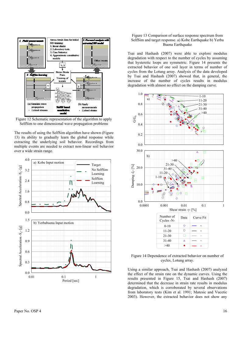
Paper No. OSP 4 16

Figure 12 Schematic representation of the algorithm to apply

SelfSim to one dimensional wave propagation problems

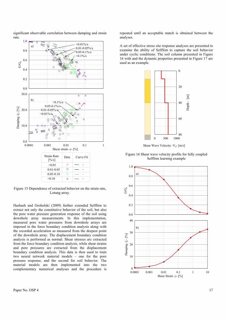
The results of using the SelfSim algorithm have shown (Figure 13) its ability to gradually learn the global response while extracting the underlying soil behavior. Recordings from multiple events are needed to extract non-linear soil behavior over a wide strain range.

0.0

0.8

1.6

2.4

3.2

4.0

Spec

tral A

ccel

erat

ion

-Sa-

[g]

0.01 0.1 1Period [sec]

0.0

0.3

0.6

0.9

1.2

1.5

Spec

tral A

ccel

erat

ion

-Sa-

[g]

TargetNo SelfSim LearningSelfSim Learning

b)

a)

Yerbabuena Input motion

Kobe Input motion

Figure 13 Comparison of surface response spectrum from SelfSim and target response. a) Kobe Earthquake b) Yerba

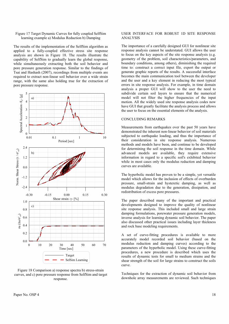
Buena Earthquake Tsai and Hashash (2007) were able to explore modulus degradation with respect to the number of cycles by assuming that hysteretic loops are symmetric. Figure 14 presents the extracted behavior of one soil layer in terms of number of cycles from the Lotung array. Analysis of the data developed by Tsai and Hashash (2007) showed that, in general, the increase of the number of cycles results in modulus degradation with almost no effect on the damping curve.

0.0

0.2

0.4

0.6

0.8

1.0

G/G

0

0.0001 0.001 0.01 0.1 1Shear strain - - [%]

0.0

10.0

20.0

30.0

Dam

ping

-- [

%]

a)

b)

1-1011-2021-3031-40

>40

1-1011-20

21-3031-40

>40

Number of Cycles -N-

0-1011-2021-3031-40>40

Data Curve Fit

Figure 14 Dependence of extracted behavior on number of cycles, Lotung array.

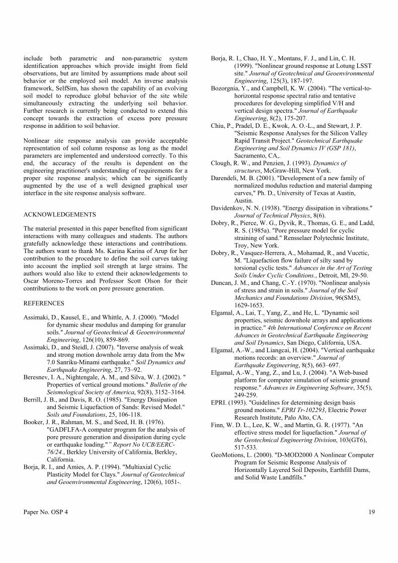
Using a similar approach, Tsai and Hashash (2007) analyzed the effect of the strain rate on the dynamic curves. Using the results presented in Figure 15, Tsai and Hashash (2007) determined that the decrease in strain rate results in modulus degradation, which is corroborated by several observations from laboratory tests (Kim et al. 1991; Matesic and Vucetic 2003). However, the extracted behavior does not show any

Paper No. OSP 4 17

significant observable correlation between damping and strain rate.

0.0

0.2

0.4

0.6

0.8

1.0

G/G

0

0.0001 0.001 0.01 0.1 1Shear strain - - [%]

0.0

10.0

20.0

30.0

Dam

ping

-- [

%]

a)

b)

<0.01%/s0.01-0.05%/s0.05-0.1%/s>0.1%/s

<0.01%/s0.01-0.05%/s

0.05-0.1%/s>0.1%/s

Strain Rate [%/s]

<0.010.01-0.050.05-0.10>0.10

Data Curve Fit

Figure 15 Dependence of extracted behavior on the strain rate,

Lotung array. Hashash and Groholski (2009) further extended SelfSim to extract not only the constitutive behavior of the soil, but also the pore water pressure generation response of the soil using downhole array measurements. In this implementation, measured pore water pressures from downhole arrays are imposed in the force boundary condition analysis along with the recorded acceleration as measured from the deepest point of the downhole array. The displacement boundary condition analysis is performed as normal. Shear stresses are extracted from the force boundary condition analysis, while shear strains and pore pressures are extracted from the displacement boundary condition analysis. This data is then used to train two neural network material models – one for the pore pressure response, and the second for soil behavior. The material models are then implemented into the two complementary numerical analyses and the procedure is

repeated until an acceptable match is obtained between the analyses. A set of effective stress site response analyses are presented to examine the ability of SelfSim to capture the soil behavior under cyclic conditions. The soil column presented in Figure 16 with and the dynamic properties presented in Figure 17 are used as an example.

0 500 1000

Shear Wave Velocity -VS- [m/s]

80

60

40

20

0

Dep

th -

[m]

Figure 16 Shear wave velocity profile for fully coupled SelfSim learning example

0.0

0.2

0.4

0.6

0.8

1.0

G/G

0

a)

0.0001 0.001 0.01 0.1 1 10Shear Strain - - [%]

0

10

20

30

40

Dam

ping

- [%

]

b)

Paper No. OSP 4 18

Figure 17 Target Dynamic Curves for fully coupled SelfSim learning example a) Modulus Reduction b) Damping

The results of the implementation of the SelfSim algorithm as applied to a fully-coupled effective stress site response analysis are shown in Figure 18. The results illustrate the capability of SelfSim to gradually learn the global response, while simultaneously extracting both the soil behavior and pore pressure generation response. Similar to the findings of Tsai and Hashash (2007), recordings from multiple events are required to extract non-linear soil behavior over a wide strain range, with the same also holding true for the extraction of pore pressure response.

0.01 0.1 1 10Period [sec]

0

1

2

3

4

5

Spec

tral A

ccel

erat

ion

-Sa-

[g]

-0.30 -0.15 0.00 0.15 0.30Shear strain - - [%]

-2.4

-1.2

0.0

1.2

2.4

Nor

m. S

hear

Stre

ss (

/ ' v0

)

0 10 20 30 40 50 60 70Time [sec]

0.0

0.2

0.4

0.6

0.8

1.0

ru (

u/' v0

)

TargetSelSim Learning

c)

b)

a)

Figure 18 Comparison a) response spectra b) stress-strain curves, and c) pore pressure response from SelfSim and target

response.

USER INTERFACE FOR ROBUST 1D SITE RESPONSE ANALYSIS

The importance of a carefully designed GUI for nonlinear site response analysis cannot be understated. GUI allows the user to focus on the key aspects of the site response analysis (e.g. geometry of the problem, soil characteristics/parameters, and boundary conditions, among others), diminishing the required time to: construct a correct input file, export the output or generate graphic reports of the results. A successful interface becomes the main communication tool between the developer and the user and a key element in reducing the most typical errors in site response analysis. For example, in time domain analysis a proper GUI will show to the user the need to subdivide certain soil layers to ensure that the numerical model will not filter the higher frequencies of the input motion. All the widely used site response analysis codes now have GUI that greatly facilitate the analysis process and allows the user to focus on the essential elements of the analysis. CONCLUDING REMARKS

Measurements from earthquakes over the past 50 years have demonstrated the inherent non-linear behavior of soil materials subjected to earthquake loading, and thus the importance of their consideration in site response analysis. Numerous methods and models have been, and continue to be developed for determining the soil response in the time domain. While advanced models are available, they require extensive information in regard to a specific soil's exhibited behavior while in most cases only the modulus reduction and damping curves are available. The hyperbolic model has proven to be a simple, yet versatile model which allows for the inclusion of effects of overburden pressure, small-strain and hysteretic damping, as well as modulus degradation due to the generation, dissipation, and redistribution of excess pore pressures. The paper described many of the important and practical developments designed to improve the quality of nonlinear site response analysis. This included small and large strain damping formulations, porewater pressure generation models, inverse analysis for learning dynamic soil behavior. The paper also discussed other practical issues including layer thickness and rock base modeling requirements. A set of curve-fitting procedures is available to more accurately model recorded soil behavior (based on the modulus reduction and damping curves) according to the parameters of the hyperbolic model. Using these curve-fitting procedures, a new procedure is described which uses the results of dynamic tests for small to medium strains and the shear strength of the soil for large strains to construct the soils curve. Techniques for the extraction of dynamic soil behavior from downhole array measurements are reviewed. Such techniques

Paper No. OSP 4 19

include both parametric and non-parametric system identification approaches which provide insight from field observations, but are limited by assumptions made about soil behavior or the employed soil model. An inverse analysis framework, SelfSim, has shown the capability of an evolving soil model to reproduce global behavior of the site while simultaneously extracting the underlying soil behavior. Further research is currently being conducted to extend this concept towards the extraction of excess pore pressure response in addition to soil behavior. Nonlinear site response analysis can provide acceptable representation of soil column response as long as the model parameters are implemented and understood correctly. To this end, the accuracy of the results is dependent on the engineering practitioner's understanding of requirements for a proper site response analysis; which can be significantly augmented by the use of a well designed graphical user interface in the site response analysis software.

ACKNOWLEDGEMENTS

The material presented in this paper benefited from significant interactions with many colleagues and students. The authors gratefully acknowledge these interactions and contributions. The authors want to thank Ms. Karina Karina of Arup for her contribution to the procedure to define the soil curves taking into account the implied soil strength at large strains. The authors would also like to extend their acknowledgements to Oscar Moreno-Torres and Professor Scott Olson for their contributions to the work on pore pressure generation. REFERENCES

Assimaki, D., Kausel, E., and Whittle, A. J. (2000). "Model for dynamic shear modulus and damping for granular soils." Journal of Geotechnical & Geoenvironmental Engineering, 126(10), 859-869.

Assimaki, D., and Steidl, J. (2007). "Inverse analysis of weak and strong motion downhole array data from the Mw 7.0 Sanriku-Minami earthquake." Soil Dynamics and Earthquake Engineering, 27, 73–92.

Beresnev, I. A., Nightengale, A. M., and Silva, W. J. (2002). " Properties of vertical ground motions." Bulletin of the Seismological Society of America, 92(8), 3152–3164.

Berrill, J. B., and Davis, R. O. (1985). "Energy Dissipation and Seismic Liquefaction of Sands: Revised Model." Soils and Foundations, 25, 106-118.

Booker, J. R., Rahman, M. S., and Seed, H. B. (1976). "GADFLFA-A computer program for the analysis of pore pressure generation and dissipation during cycle or earthquake loading."�” Report No UCB/EERC-76/24., Berkley University of California, Berkley, California.

Borja, R. I., and Amies, A. P. (1994). "Multiaxial Cyclic Plasticity Model for Clays." Journal of Geotechnical and Geoenvironmental Engineering, 120(6), 1051-.

Borja, R. I., Chao, H. Y., Montans, F. J., and Lin, C. H. (1999). "Nonlinear ground response at Lotung LSST site." Journal of Geotechnical and Geoenvironmental Engineering, 125(3), 187-197.

Bozorgnia, Y., and Campbell, K. W. (2004). "The vertical-to-horizontal response spectral ratio and tentative procedures for developing simplified V/H and vertical design spectra." Journal of Earthquake Engineering, 8(2), 175-207.

Chiu, P., Pradel, D. E., Kwok, A. O.-L., and Stewart, J. P. "Seismic Response Analyses for the Silicon Valley Rapid Transit Project." Geotechnical Earthquake Engineering and Soil Dynamics IV (GSP 181), Sacramento, CA,.

Clough, R. W., and Penzien, J. (1993). Dynamics of structures, McGraw-Hill, New York.

Darendeli, M. B. (2001). "Development of a new family of normalized modulus reduction and material damping curves," Ph. D., University of Texas at Austin, Austin.

Davidenkov, N. N. (1938). "Energy dissipation in vibrations." Journal of Technical Physics, 8(6).

Dobry, R., Pierce, W. G., Dyvik, R., Thomas, G. E., and Ladd, R. S. (1985a). "Pore pressure model for cyclic straining of sand." Rensselaer Polytechnic Institute, Troy, New York.

Dobry, R., Vasquez-Herrera, A., Mohamad, R., and Vucetic, M. "Liquefaction flow failure of silty sand by torsional cyclic tests." Advances in the Art of Testing Soils Under Cyclic Conditions., Detroit, MI, 29-50.

Duncan, J. M., and Chang, C.-Y. (1970). "Nonlinear analysis of stress and strain in soils." Journal of the Soil Mechanics and Foundations Division, 96(SM5), 1629-1653.

Elgamal, A., Lai, T., Yang, Z., and He, L. "Dynamic soil properties, seismic downhole arrays and applications in practice." 4th International Conference on Recent Advances in Geotechnical Earthquake Engineering and Soil Dynamics, San Diego, California, USA.

Elgamal, A.-W., and Liangcai, H. (2004). "Vertical earthquake motions records: an overview." Journal of Earthquake Engineering, 8(5), 663–697.

Elgamal, A.-W., Yang, Z., and Lu, J. (2004). "A Web-based platform for computer simulation of seismic ground response." Advances in Engineering Software, 35(5), 249-259.

EPRI. (1993). "Guidelines for determining design basis ground motions." EPRI Tr-102293, Electric Power Research Institute, Palo Alto, CA.

Finn, W. D. L., Lee, K. W., and Martin, G. R. (1977). "An effective stress model for liquefaction." Journal of the Geotechnical Engineering Division, 103(GT6), 517-533.

GeoMotions, L. (2000). "D-MOD2000 A Nonlinear Computer Program for Seismic Response Analysis of Horizontally Layered Soil Deposits, Earthfill Dams, and Solid Waste Landfills."

Paper No. OSP 4 20

Gerolymos, N., and Gazetas, G. (2005). "Constitutive model for 1-D cyclic soil behaviour applied to seismic analysis of layered deposits." Soils and Foundation, 45(3), 147-159.

Ghaboussi, J., and Dikmen, S. U. (1984). "Effective stress analysis of seismic response and liquefaction: Case studies,." Journal of Geotechnical Engineering, ASCE, 110(5), 645–658.

Ghaboussi, J., Pecknold, D. A., Zhang, M., and Haj-Ali, R. (1998). "Autoprogressive training of neural network constitutive models." International Journal for Numerical Methods in Engineering, 42(1), 105-126.

Glaser, S. D., and Baise, L. G. (2000). "System identification estimation of soil properties at the Lotung site." Soil Dynamics and Earthquake Engineering, 19, 521-531.

Green, R. A., Mitchell, J. K., and Polito, C. P. "An energy-based pore pressure generation model for cohesionless soils.." John Booker Memorial Symp.�—Developments in Theoretical Geomechanics, Rotterdam, The Netherlands, 383–390.

Hardin, B. O., and Drnevich, V. P. (1972a). "Shear modulus and damping in soils: Design equations and curves." Journal of Soil Mechanics and Foundations, 98(SM7), 289-324.

Hardin, B. O., and Drnevich, V. P. (1972b). "Shear modulus and damping in soils: Measurement and parameter effects." Journal of Soil Mechanics and Foundation Engineering Division, 98(SM6), 603-624.

Harichance, Z., Afra, H., and Elachachi, S. M. (2005). "An identification procedure of soil profile characteristics from two free field acclerometer records." Soil Dynamics and Earthquake Engineering, 25, 431-438.

Hashash, Y. M., and Groholski, D. "Extraction of dynamic pore water pressure generation behavior via inverse analysis in seismic site response modeling." 1st International Symposium on Computational Geomechanics (ComGeo I), ,, Juan-les-Pins, Cote d'Azur, France.

Hashash, Y. M. A. (2009). "DEEPSOIL V 3.7, Tutorial and User Manual. 2002-2009." University of Illinois at Urbana-Champaign, Urbana, Illinois.

Hashash, Y. M. A., and Park, D. (2001). "Non-linear one-dimensional seismic ground motion propagation in the Mississippi embayment." Engineering Geology, 62(1-3), 185-206.

Hudson, M., Idriss, I. M., and Beikae, M. (2003). QUAD4M : a computer program to evaluate the seismic response of soil structures using finite element procedures and incorporating a compliant base. rev. 2003, Center for Geotechnical Modeling Dept. of Civil and Environmental Engineering University of California Davis.

Hudson, M., Idriss, I.M., and Beikae, M. 1994. (1994). "QUAD4M - A computer program to evaluate the seismic response of soil structures using finite element procedures and incorporating a compliant base." Center for Geotechnical Modeling,

Department of Civil and Environmental Engineering, University of California, Davis, CA., Davis, CA.

Idriss, I. M., and Sun, J. I. (1992). "SHAKE91: A computer program for conducting equivalent linear seismic response analyses of horizontally layered soil deposits." Department of Civil and Environmental Engineering, University of California Davis.

Ishibashi, I., and Zhang, X. (1993). "Unified dynamic shear moduli and damping ratios of sand and clay." Soils and Foundations, 33(1), 182-191.

Ishihara, K., and Kasuda, K. "Dynamic strenght of cohesive soil." Proceedings of the Sixth Budapest Conference on Soil Mechanics and Foundation Engineering, Budapest, Hung.

Ishihara, K., Lysmer, J., Yasuda, S., and Hirao, H. (1976). " Prediction of liquefaction in sand deposits during earthquakes." Soils and Foundations, 16(1), 1-16.

Iwasaki, T., Tatsuoka, F., and Takagi, Y. (1978). "Shear moduli of sands under cyclic torsional shear loading." Soils and Foundations, 18(1), 32-56.

Kim, D. S., Stokoe, K. H., and Hudson, W. R. (1991). "Deformational characteristics of soils at small to intermediate strains from cyclic tests." 1177-3, Center of Transportation Research, Bureau of Engineering Research, Austin Texas.

Kokusho, T. (1980). "Cyclic triaxial test of dynamic soil properties for wide strain range." Soils and Foundations, 20(2), 45-60.

Kondner, R. L., and Zelasko, J. S. "Hyperbolic stress-strain formulation of sands." Second pan American Conference on Soil Mechanics and Foundation Engineering, Sao Paulo, Brazil, 289-324.

Kramer, S. L. (1996). Geotechnical earthquake engineering, Prentice Hall, Upper Saddle River, N.J.

Kwok, A. O. L., Stewart, J. P., Hashash, Y. M. A., Matasovic, N., Pyke, R., Wang, Z., and Yang, Z. (2007). "Use of exact solutions of wave propagation problems to guide implementation of nonlinear, time-domain ground response analysis routines." ASCE Journal of Geotechnical and Geoenvironmental Engineering, in press.

Lai, C. G., and Rix, G. J. (1998). "Simultaneous Inversion of Rayleigh Phase Velocity and Attenuation for Near-Surface Site Characterization." Georgia Institute of Technology.

Laird, J. P., and Stokoe, K. H. (1993). "Dynamic properties of remolded and undisturbed soil samples test at high confining pressure." GR93-6, Electric Power Research Institute.

Lee, K. L., and Albaisa, A. S. (1974). "Earthquake induced settlements in saturated sands." Journal of Geotechnical Engineering, ASCE, 100(GT4), 387-406.

Lee, M. K., and Finn, W. D. L. (1975). "DESRA-1, Program for the dynamic effective stress response analysis of soil deposits including liquefaction evaluation." Soils Mechanics No 36, Department of Civil Engineering,

Paper No. OSP 4 21

University of British Columbia, Vancouver, B.C. Canada.

Lee, M. K., and Finn, W. D. L. (1978). "DESRA-2, Dynamic effective stress response analysis of soil deposits with energy transmitting boundary including assessment of liquefaction potential." Soil Mechanics Series, No. 36, Department of Civil Engineering, University of British Columbia, Vancouver, Canada.

Li, X., Wang, Z. L., and Shen, C. K. (1997). "SUMDES. A nonlinear procedure for response analysis of horizontally layered sites subjected to multi-directional earthquake loading." Department of Civil Engineering, University of California at Davis.

Liu, M., and Gorman, D. G. (1995). "Formulation of Rayleigh damping and its extensions." Computers and Structures, 57(2), 277-285.

Martin, P. P., and Seed, H. B. (1978). "MASH: a computer program for the non-linear analysis of vertically propagating shear waves in horizontally layered deposits." University of California at Berkeley, San Francisco.

Masing, G. "Eignespannungen und Verfestigung beim Messing." Second International Congress on Applied Mechanics, Zurich, Switzerland, 332-335.

Matasovic, N. (1993). "Seismic response of composite horizontally-layered soil deposits," Ph.D. Thesis, University of California, Los Angeles.

Matasovic, N., and Vucetic, M. (1993). "Cyclic Characterization of Liquefiable Sands." ASCE Journal of Geotechnical and Geoenvironmental Engineering, 119(11), 1805-1822.

Matesic, L., and Vucetic, M. (2003). "Strain-rate effect on soil secant shear modulus at small cyclic strains." J. Geotech. and Geoenvir. Engrg, 129(6), 536-539.

McKenna, F., and Fenves, G. L. (2001). "The OpenSees Command Language Manual: version 1.2." PEER Center, University of California at Berkely.

Mok, C.-M., Chang, C.-Y., and Legaspi, D. E. "Site response analyses of vertical excitation." Geotechnical Earthquake Engineering and Soil Dynamics III, Seatlle, WA, 739-753.

Moreno-Torres, O., Hashash, Y. M. A., and Olson, S. M. "A simplified coupled soil-pore water pressure generation for use in site response analysis." GeoFlorida Advances in Analysis, Modeling & Design, West Palm Beach, Florida, USA.

Muravskii, G. (2005). "On description of hysteretic behaviour of materials." International Journal of Solids and Structures, 42, 2625-2644.

Muravskii, G., and Frydman, S. (1998). "Site response analysis using a nonlinear hysteretic model." Soil Dynamics and Earthquake Engineering, 17, 227–238.

Newmark, N. M. (1959). "A Method of Computation for Structural Dynamics." Journal of the Engineering Mechanics Division, 85, 67-94.

Nishi, K., Tohma, J., and Kanatani, M. "Effective stress analysis for level sand deposits with cyclic mobility."

5th Internationa Conference on Numerical Methods in Geomechanics, Nagoya, Japan.

Papazoglou, A. J., and Elnashai, A. S. (1996). "Analytical and field evidence of the damaging effect of vertical earthquake ground motion." Journal of Earthquake Engineering and Structural Dynamics, 25(10), 1109–1137.

Park, D., and Hashash, Y. M. A. (2004). "Soil damping formulation in nonlinear time domain site response analysis." Journal of Earthquake Engineering, 8(2), 249-274.

Park, D., and Hashash, Y. M. A. (2008). "Rate-dependent soil behavior in seismic site response analysis." Canadian Geotechnical Journal, 45(4), 454-446.

Phillips, C., and Hashash, Y. M. (2009). "Damping formulation for nonlinear 1D site response analyses." Soil Dynamics and Earthquake Engineering, 29(7), 1143–1158.

Polito, C. P., Green, R. A., and Lee, J. H. (2008). "Pore pressure generation models for sands and silty soils subjected to cyclic loading." Journal of Geotechnical and Geoenvironmental Engineering, 134(10), 1490-1500.

Press, W. H., Teukolsky, S. A., Vetterling, W. T., and Flannery, B. P. (1992). Numerical Recipes in FORTRAN 77 The Art of Scientific Computing, Cambridge University Press, Cambridge, UK.

Prevost, J. H. (1977). "Mathematical modeling of monotonic and cyclic undrained clay behavior." International Journal of Numerical and Analytical Methods in Geomechanics, 1(2), 195-216.

Prevost, J. H. (1989). "DYNA1D: A computer program for nonlinear site response analysis, technical documentation."", National Center of Earthquake Engineering Research, Sunny at Buffalo, NY.

Prevost, J. H., and Keane, C. M. (1990). "Multimechanism Elasto-Plastic Model for Soils." Journal of Engineering Mechanics, 116(9), 1924-1945.

Puzrin, A. M., and Burland, J. B. (1996). "A logarithmic stress–strain function for rocks and soils." Geotechnique, 46(1), 157–164.

Pyke, R. (2000). "TESS: A computer program for nonlinear ground response analyses." TAGA Engineering Systems and Software, Lafayette, California.

Pyke, R. M. (1979). "Nonlinear soil models for irregular cyclic loadings." Journal of the Geotechnical Engineering Division, 105(GT6), 715-726.

Pyke, R. M., Seed, H. B., and Chan, C. K. (1975). "Settlement of sands under multidirectional shaking." Journal of Geotechincal Engineering Division, ASCE, 101(GT4), 379-398.

Ramberg, W., and Osgood, W. R. (1943). "Description of stress-strain curves by three parameters." Technical Note No. 902, National Advisory Committee For Aeronautics, Washington DC.

Rayleigh, J. W. S., and Lindsay, R. B. (1945). The theory of sound, Dover Publications, New York.

Paper No. OSP 4 22

Schnabel, P. B., Lysmer, J. L., and Seed, H. B. (1972). "SHAKE: A computer program for earthquake response analysis of horizontally layered sites." EERC-72/12, Earthquake Engineering Research Center, Berkeley, CA.

Seed, H. B., and Idriss, I. M. (1969). "Influence of soil conditions on ground motions during earthquakes." ASCE J Soil Mech Found Div, 95, 99-137.

Seed, H. B., Idriss, I. M., Makdisi, F., and Bannerjee, N. (1975). "Representation of irregular stress time histories by equivalent uniform stress series in liquefaction analyses." Report No. UCB/EERC/75-29, Earthquake Engineering Research Center, University of California, Berkeley, California.

Seed, H. B., Pyke, R. M., and Martin, G. R. (1978). "Effect of multi-directional shaking on pore-pressure development in sands." Journal Geotechnical Engineering Division, ASCE, 104(GT1), 27-44.

Sheahan, T. C., Ladd, C. C., and J.T.Germaine. (1996). "Rate Dependent Undrained Shear Behavior of Saturated Clay." Journal of Geotechnical and Geoenvironmental Engineering, 122(2), 99-108.

Sidarta, D., and Ghaboussi, J. (1998). "Modelling constitutive behavior of materials from non-uniform material tests." Computers and Geotechnics, 22(1), 53-71.

Silver, M. L., and Seed, H. B. (1971). "Volume changes in snads during cyclic loading." Journal of Soil Mechanics and Foundation Division, American Society of Civil Engineers, 97(SM9), 1174-1178.

Stewart, J., and Kwok, A. O. L. "Nonlinear seismic ground response analysis: Code usage protocols and verification against vertical array data." Geotechnical Earthquake Engineering and Soil Dynamics IV Congress 2008 - Geotechnical Earthquake Engineering and Soil Dynamics, GSP 181.

Streeter, V. L., Wylie, E. B., and Richart, F. E. (1974). "Soil motion computation by characteristic method." Journal of the Geotechnical Engineering Division, 100(GT3), p 247-263.

Sugito, M., Goda, H., and Masuda, T. (1994). "Frequency dependent equi-linearized technique for seismic response analysis of multi-layered ground." Doboku Gakkai Rombun-Hokokushu/Proceedings of the Japan Society of Civil Engineers, 493(3-2), 49-58.

Tsai, C.-C., and Hashash, Y. M. A. (2007). "A novel framework integrating downhole array data and site response analysis to extract dynamic soil behavior." Soil Dynamics and Earthquake Engineering, 28(3), 181-197.

Vucetic, M. (1986). "Pore pressure buildup and liquefaction at level sand sites during earthquakes," Rensselaer Polytechnic Institute, Troy, N. Y.

Vucetic, M., and Dobry, R. (1988). "Cyclic triaxial strain-controlled testing of liquefiable sands." Advanced Triaxial Testing of Soil and Rock, ASTM STP 977, American Society for Testing and Materials, Philadelphia, 475-485.

Watabe, M., Tohido, M., Chiba, O., and Fukuzawa, R. "Peak accelerations and response spectra of vertical strong motions from near-field records in USA,." Eighth Japan Earthquake Engineering Symposium, Tokyo, Japan, 301-306.

Wilson, E. (2005). "Dynamic analysis by numerical integration." Computers and Structures Inc., San Francisco, California.

Yang, Z. (2000). "Numerical Modeling of Earthquake Site Response Including Dilation and Liquefaction.," Columbia University, NY, New York.

Youd, T. L. (1972). "Compaction of sands by repeated shear straining. J." Journal of Soil Mechanics and Foundation Division, American Society of Civil Engineers, 98, 709–725.

Zeghal, M., and Elgamal, A.-W. (1993). "Lotung sites: downhole seismic data analysis." Electric Power Research Institute, Palo Alto, Calif,.