Recent advances in Astrophysical MHD

Jim Stone Department of Astrophysical Sciences

& PACMPrinceton University, USA

Recent collaborators:Tom Gardiner (Cray Research)John Hawley (UVa)Peter Teuben (UMd)

Eagle nebula (M16)

Numerical methods for MHD are crucial for understanding the dynamics of astrophysical plasmas.

Modern schemes solve the equations of ideal MHD in conservative form

Many schemes are possible: central schemesWENO schemesTVD schemes

We have adopted finite-volume techniques using Godunov’s method.

C

Basic Algorithm: Discretization

Bx

By

EV

Scalars and velocity at cell centers

Magnetic field at cell faces

Cell-centered quantities volume-averaged

Face centered quantities area-averaged

Area averaging is the natural discretization for the magnetic field.

For pure hydrodynamics of ideal gases, exact/efficient nonlinearRiemann solvers are possible.

In MHD, nonlinear Riemann solvers are complex because:1. There are 3 wave families in MHD – 7 characteristics2. In some circumstances, 2 of the 3 waves can be degenerate

(e.g. VAlfven = Vslow )

Equations of MHD are not strictly hyperbolic (Brio & Wu, Zachary & Colella)

Thus, in practice, MHD Godunov schemes use approximate and/or linearized Riemann solvers.

Key element of Godunov method is Riemann solver

Many possible approximations are possible:

1. Roe’s method – keeps all 7 characteristics, but treats each as a simple wave.

2. Harten-Lax-van Leer (HLLE) method – keeps only largest and smallest characteristics, averages intermediate states in-between.

3. HLLD method – Adds entropy and Alfven wave back into HLLE method, giving four intermediate states.

Good resolution of all wavesRequires characteristic decomposition in conserved variablesExpensive and difficult to add new physicsDoes not preserve positivity

Very simple and efficientGuarantees positivityVery diffusive for contact discontinuities

Reasonably simple and efficientGuarantees positivityBetter resolution of contact discontinuities

Keeping B = 0

1. Do nothing. Assume errors remain small and bound.

2. Evolve B using vector potential defined through B=

3. Remove solenoidal part of B using “flux-cleaning”. That is, set B B – where + B = 0

4. Use Powell’s “8-wave solver” (adds div(B) source terms)

5. Evolve integral form of induction equation so as to conserve magnetic flux (constrained transport).

.

2

Requires taking second difference numerically to compute Lorentz force

Requires solving elliptic PDE every timestep – expensiveMay smooth discontinuities in B

Gives wrong jump conditions for some shock problems

Requires staggered grid for B (although see Toth 2000)

The CT Algorithm

• Finite Volume / Godunov algorithm gives E-field at face centers.

• “CT Algorithm” defines E-field at grid cell corners.

• Arithmetic averaging: 2D plane-parallel flow does not reduce to equivalent 1D problem

• Algorithms which reconstruct E-field at corner are superior Gardiner & Stone 2005

Ez,i 1 2,j 1

Ez,i 1 2,j

Ez,i , j 1 2 Ez,i 1, j 1 2

Ez,i 1 2,j 1 2

Simple advection tests demonstrate differences

Field Loop Advection (106): MUSCL - Hancock

Arithmetic average Gardiner & Stone 2005(Balsara & Spicer 1999)

QuickTime™ and aGIF decompressor

are needed to see this picture.

QuickTime™ and aGIF decompressor

are needed to see this picture.

Which Multidimensional Algorithm?

CornerTransportUpwind [Colella 1991] (12 R-solves)• Optimally Stable, CFL < 1

• Complex & Expensive for MHD...

CTU (6 R-solves)• Stable for CFL < 1/2

• Relatively Simple...

MUSCL-Hancock• Stable for CFL < 1/2

• Very Simple, but diffusive...

Verification: Linear Wave Convergence(2N x N x N) Grid

Validation: Hydro RT instability

2562 x 512 grid

Random perturbations

Isosurface and slices of density

QuickTime™ and aGIF decompressor

are needed to see this picture.

Dimonte et al, Phys. Fluids (2004) have used time evolution of rising “bubbles” and falling “spikes” from experiments to validate hydro codes:

Asymptotic slope too small in ALL codes by about factor 2

Probably because of mixing at grid scale

Comparison with expts. using miscible fluids much better

experiment

Application: 3D MHD RT instability

2562 x 512 grid

Random perturbations

Isosurface and slices of density

B = (Bx, 0, 0) crit = Lx/2

QuickTime™ and aGIF decompressor

are needed to see this picture.

Codes are publicly available

Download a copy from

www.astro.princeton.edu/~jstone/athena.html

Current status:• 1D version publicly available• 2D version publicly available• 3D version will be released in ~1 month

• Latest project is funded by NSF ITR; source code public.• Code, documentation, and training material posted on web.• 1D, 2D, and 3D versions are/will be available.

EXAMPLE APPLICATION: MHD of Accretion disks

e.g., mass transfer in a close binary

If accreting plasma has any angular momentum, it will form a rotationally supported disk

L r1/2

r-3/2

Thereafter, accretion can only occur if angular momentum is transported outwards.

• microscopic viscosity too small• anomalous (turbulent?) viscosity required

MHD turbulence driven by magnetorotational instability (MRI) dominates

Profiles of specific angular momentum (L) and orbital frequency () for Keplerian disk:

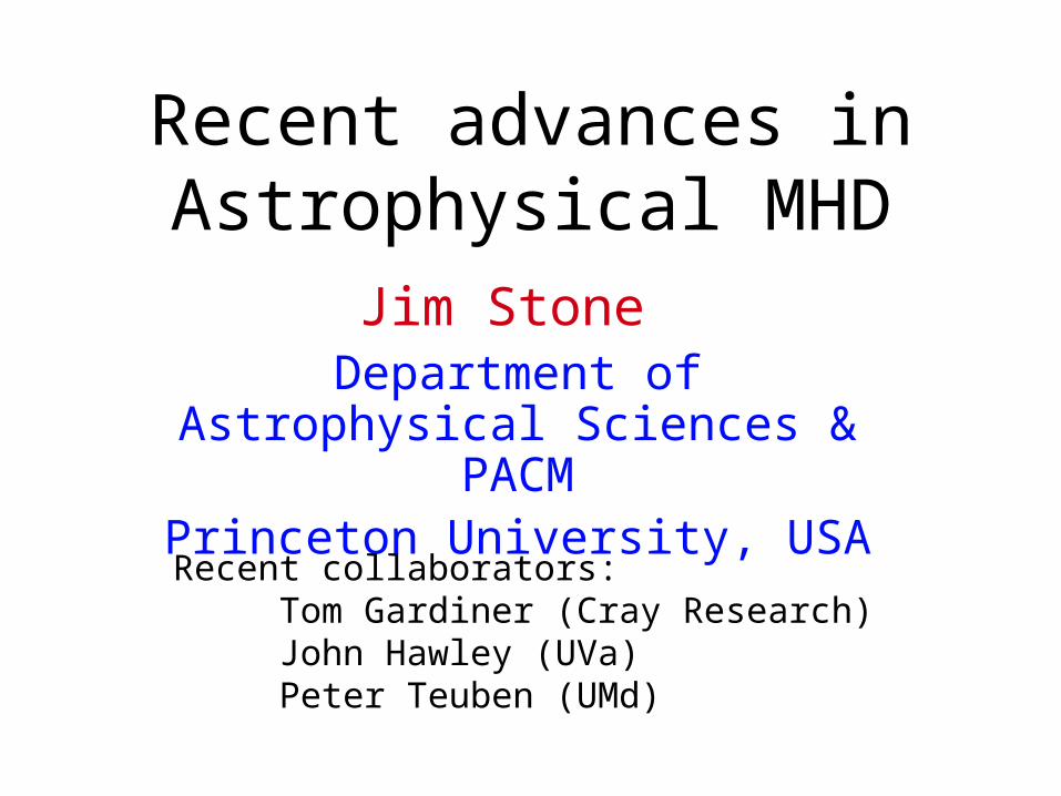
Start from a vertical field with zero net flux: Bz=B

0sin(2x)

Sustained turbulence not possible in 2D – dissipation rateafter saturation is sensitive to numerical dissipation: Code Test

Animation of angular velocity fluctuations: Vy=V

y+1.5

0x

CTU with 3rd order reconstruction, 2562 grid, min

=4000, orbits 2-10

QuickTime™ and aGIF decompressor

are needed to see this picture.

Magnetic Energy Evolution

Numerical dissipation is ~1.5 times smaller withCTU & 3rd order reconstruction than Zeus.

3D MRIAnimation of angular velocity fluctuations: V

y=V

y+1.5

0x

Initial Field Geometry is Uniform By

CTU with 3rd order reconstruction, 128 x 256 x 128 Grid

min= 100, orbits 4-20

In 3D, sustained turbulenceQuickTime™ and a

Video decompressorare needed to see this picture.

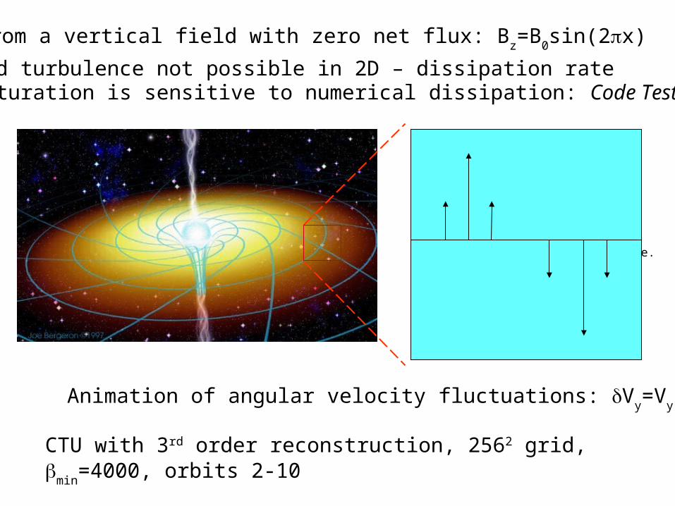
Stress & Energy for <Bz> 0

No qualitative difference with ZEUS results (Hawley, Gammie, & Balbus 1995)

Vertical structure of stratified disks

Now using static nested-grids to refine midplane of thin disks with cooling in shearing box

Next step towards nested-grid global models

Density Angular momentum fluctuations

Future Extensions to Algorithm• Curvilinear coordinates• Nested and adaptive grids (already implemented)• full-transport radiation hydrodynamics (w. Sekora)• non-ideal MHD (w. Lemaster)• special relativistic MHD (w. MacFayden)

Star formation Global models of accretion disks

Future Applications