© 1999 Macmillan Magazines Ltd

letters to nature

NATURE | VOL 399 | 17 JUNE 1999 | www.nature.com 673

wavelength using Eagle Eye II and a top-mounted 350-nm ultravioletilluminator (Stratagene). Automated colony detection and individual fluorescenceintensity measurements were performed using Optimas 5.0 image analysissoftware (Optimas) with a weighted score of 27,000 grey scale. A blue band-passfilter (430–470 nm), 4× lens zoom level, and 1/10 s CCD exposure time wereused. Typical colony diameters were ,0.4–0.8 mm. Scanned images werefurther processed by configuring overall thresholding, geometry recognition,intensity quantification, global and local segmentation, and cutting edges toreduce background fluorescence.Hydroxylation activity measurements. Naphthalene and 3-PPA whole-cellhydroxylation activities were measured in 200-ml reactions in a 96-wellmicrotitre plate. P450cam þ HRP cells grown in 50-ml flasks were collected bycentrifugation (Beckman CS SR) at 3,350 r.p.m. and resuspended in 1 ml of0.1 M sodium phosphate buffer (pH 9.0). A 50-ml aliquot of the cell solutionwas added to the reaction mixtures (total 200 ml) containing 25% ethanol, 3-PPA (0.5 mM) or naphthalene (6 mM), and H2O2 (10 mM) in the same buffer.Fluorescence was measured in a 96-well microfluorimeter (HTS 7000, PerkinElmer).

For regioselectivity comparisons, reactions were carried out using cellsexpressing P450cam and no HRP. Cells grown in 50-ml flasks were collected bycentrifugation and gently resuspended in 5 ml of 0.1 M phosphate buffer (pH9.0) containing 5% (v/v) ethanol, 50 mM naphthalene and 50 mM H2O2. After1 h incubation, the products were extracted with 2 ml of chloroform, and thephases were separated by centrifugation. Residual proteins and salt wereremoved by ethanol precipitation (3×). The final extracts were spotted on a thin-layer silica plate (Kieselgel 60F254, Merck, Darmstadt, Germany) and developedwith 94% (v/v) chloroform/methanol. Spots corresponding to 1-naphthol and1,3-DHN were identified by comparison to the pure compounds andconfirmed using an electrospray ionization-quadrupole ion trap massspectrometer (LCQ, Finnigan, Bremen, Germany). No other hydroxylatednaphthalenes were observed at significant concentrations in the productmixtures. Relative concentrations were determined from the integrated spotdensities on the thin layer chromatogram (AlphaImager 2000).Mutagenic PCR and StEP recombination. Mutagenic PCR was performed in a100 ml reaction as described31, using 0.7 mM MnCl2, 14 pmol of each primer, 5 unitsof Taq polymerase (Boehringer Mannheim), 0.01% gelatin, 20 pmol of templateDNA (P450cam_pCWori(+)). PCR was performed in a thermocycler (PTC200, MJResearch, Waltham, Massachusetts) for 30 cycles (94 8C, 30 s; 45 8C, 30 s; 72 8C,2 min). Sequences of forward and reverse primers are 59-CATCGATGCTTAGGAGGTCATATG-39 and 59-TCATGTTTGACAGCTTATCATCGAT-39. The StEPmethod25,31 was used to recombine five mutant P450cam genes from the firstgeneration, under slightly mutagenic conditions (0.3 mM MnCl2).P450cam purification and assay. Wild-type and M7-8H P450cam were purifiedas described32. P450 content was estimated by measuring absorbance at 392 nm,with e ¼ 104 mM 2 1 cm 2 1. P450 fractions eluted from a Q–Sepharose(Pharmacia) column were pooled (average purity, A392/A280:1.4–1.6) andwashed three times with fresh 10 mM Tris buffer (pH 7.3). Assay conditionswere: (200 ml total) 100 mM dibasic phosphate buffer (pH 9.0), 15% (v/v) pureethanol, 30 mM naphthalene, 1.75 mM HRP (E.C.1.11.1.7, type II; Sigma),100 mM H2O2, 0.031 mM (or 0.282 mg) purified P450. Fluorescence at 465 nm(excitation at 350 nm) was measured in a 96-well microfluorimeter. One unit isdefined as the value of 1 a.u. fluorescence increase at 465 nm per min per mgP450.

Received 14 December 1998; accepted 11 May 1999.

1. Nelson, D. R. et al. P450 superfamily: update on new sequences, gene mapping, accession numbersand nomenclature. Pharmacogenetics 6, 1–42 (1996).

2. Cerniglia, C. E. Biodegradation of polycyclic aromatic hydrocarbons. Biodegradation 3, 351–368(1992).

3. Cook, D. L. & Atkins, W. M. Enhanced detoxication due to distributive catalysis and toxic thresholds:a kinetic analysis. Biochemistry 36, 10801–10806 (1997).

4. Waxman, D. J. & Chang, T. K. H. in Cytochrome P450: Structure, Mechanism and Biochemistry 2nd edn(ed. Ortiz de Montellano, P. R.) 391–417 (Plenum, New York, 1995).

5. Gonzalez, F. J. & Nebert, D. W. Evolution of the P450-gene superfamily—animal plant warfare,molecular drive and human genetic differences in drug oxidation. Trends Genet. 6, 182–186 (1990).

6. Sono, M., Roach, M. P., Coulter, E. D. & Dawson, J. H. Heme-containing oxygenases. Chem. Rev. 96,2841–2887 (1996).

7. Jounaidi, Y., Hecht, J. E. D. & Waxman, D. J. Retroviral transfer of human cytochrome P450 genes foroxazaphosphorine-based cancer gene therapy. Cancer Res. 58, 4391–4401 (1998).

8. Wackett, L. P., Sadowsky, M. J., Newman, L. M., Hur, H.-G. & Li, S. Metabolism of polyhalogenatedcompounds by a genetically engineered bacterium. Nature 368, 627–629 (1994).

9. Faber, K. Biotransformations in Organic Chemistry 208–220 (Springer, Berlin, 1997).

10. Duport, C., Spagnoli, R., Degryse, E. & Pompon, D. Self-sufficient biosynthesis of pregnenolone andprogesterone in engineered yeast. Nature Biotechnol. 16, 186–189 (1998).

11. Arnold, F. H. Design by directed evolution. Acc. Chem. Res. 31, 125–131 (1998).12. Nordblom, G. D., White, R. E. & Coon, M. J. Studies on hydroperoxide-dependent substrate

hydroxylation by purified liver microsomal cytochrome P450. Arch. Biochem. Biophys. 175, 524–533 (1976).

13. Hrycay, E. G., Gustafsson, J.-A., Ingelman-Sundberg, M. & Ernster, L. Sodium periodate, sodiumchlorite, organic hydroperoxides and hydrogen peroxide as hydroxylating agents in steroid hydro-xylation reactions catalyzed by partially purified cytochrome P450. Biochem. Biophys. Res. Commun.66, 209–216 (1975).

14. Hummel, W. & Kula, M.-R. Dehydrogenases for the synthesis of chiral compounds. Eur. J. Biochem.184, 1–13 (1989).

15. Seelbach, K. et al. A novel, efficient regenerating method of NADPH using a new formatedehydrogenase. Tetrahedron Lett. 37, 1377–1380 (1997).

16. Henriksen, A. et al. Structural interactions between horseradish peroxidase C and the substratebenzhydroxamic acid determined by X-ray crystallography. Biochemistry 37, 8054–8060 (1998).

17. Lin, Z., Thorsen, T. & Arnold, F. H. Functional expression of horseradish peroxidase in Escherichia coliby directed evolution. Biotechnol. Prog. 15, 467–471 (1999).

18. Gunsalus, I. C., Meeks, J. R., Lipscomb, J. D., Debrunner, P. G. & Munck, E. in Molecular Mechanismsof Oxygen Activation (ed. Hayaishi, O.) 559–613 (Academic, New York, 1974).

19. England, P. A., Harford-Cross, C. F., Stevenson, J.-A., Rouch, D. A. & Wong, L.-L. The oxidation ofnaphthalene and pyrene by cytochrome P450cam. FEBS Lett. 424, 271–274 (1998).

20. Poulos, T. L. & Raag, R. Cytochrome P450cam: crystallography, oxygen activation, and electrontransfer. FASEB J. 6, 674–679 (1992).

21. Graham-Lorence, S. & Peterson, J. A. P450s: Structural similarities and functional differences. FASEBJ. 10, 206–214 (1996).

22. Denu, J. M. & Tanner, K. G. Specific and reversible inactivation of protein tyrosine phosphatases byhydrogen peroxide: evidence for a sulfenic acid intermediate and implications for redox regulation.Biochemistry 37, 5633–5642 (1998).

23. van Deurzen, M. P. J., van Rantwijk, F. & Sheldon, R. A. Selective oxidations catalyzed by peroxidases.Tetrahedron 53, 13183–13220 (1997).

24. Crameri, A., Raillard, S.-A., Bermudez, E. & Stemmer, W. P. C. DNA shuffling of a family of genes fromdiverse species accelerates directed evolution. Nature 391, 288–291 (1998).

25. Zhao, H., Giver, L., Shao, Z., Affholter, J. A. & Arnold, F. H. Molecular evolution by staggeredextension process (StEP) in vitro recombination. Nature Biotechnol. 16, 258–261 (1998).

26. Moore, J. C. & Arnold, F. H. Directed evolution of a para-nitrobenzyl esterase for aqueous-organicsolvents. Nature Biotechnol. 14, 458–467 (1996).

27. Giver, L., Gershenson, A., Freskgard, P. O. & Arnold, F. H. Directed evolution of a thermostableesterase. Proc. Natl Acad. Sci. USA 95, 12809–12813 (1998).

28. Zhao, H. & Arnold, F. H. Directed evolution converts subtillisin E into a functional equivalent ofthermitase. Protein Eng. 12, 47–53 (1999).

29. McKay, C. P. & Hartman, H. Hydrogen peroxide and the evolution of oxygenic photosynthesis.Origins Life Evol. Biosphere 21, 157–163 (1991).

30. Samuilov, V. D. Photosynthetic oxygen: the role of H2O2. A review. Biochemistry (Moscow) 62, 451–454 (1997).

31. Zhao, H., Moore, J. C., Volkov, A. A. & Arnold, F. H. in Manual of Industrial Microbiology andBiotechnology 2nd edn (eds Demain, A. L. & Davies, J. E.) 597–604 (ASM Press, Washington DC,1999).

32. Unger, B. P., Gunsalus, I. C. & Sligar, S. G. Nucleotide-sequence of the Pseudomonas-putidacytochrome P-450cam gene and its expression in Escherichia-coli. J. Biol. Chem. 261, 1158–1163 (1986).

Acknowledgements. We thank J. H. Richards for encouragement and support, P. R. Ortiz de Montellanofor discussions, and G. Bandara for assistance with purification. This work was supported by theBiotechnology Research and Development Corporation and by the Office of Naval Research. H.J. receivedpartial support from the Korea Research Foundation.

Correspondence and requests for materials should be addressed to F.H.A. (e-mail: frances@cheme.caltech.edu).

Reassessmentof ice-agecoolingof the tropicaloceanandatmosphereS. W. Hostetler* & A. C. Mix†

* US Geological Survey, 200 SW 35th Street, Corvallis, Oregon 97331-5503, USA† College of Oceanic & Atmospheric Science, Ocean Administration Building 104,Oregon State University, Corvallis, Oregon 97331-5503, USA. . . . . . . . . . . . . . . . . . . . . . . . . . . . . . . . . . . . . . . . . . . . . . . . . . . . . . . . . . . . . . . . . . . . . . . . . . . . . . . . . . . . . . . . . . . . . . . . . . . . . . . . . . . . . . . . . . . . . . . . .

The CLIMAP1 project’s reconstruction of past sea surface tem-perature inferred limited ice-age cooling in the tropical oceans.This conclusion has been controversial, however, because of thegreater cooling indicated by other terrestrial and ocean proxydata2–6. A new faunal sea surface temperature reconstruction,calibrated using the variation of foraminiferal species throughtime, better represents ice-age faunal assemblages and so revealsgreater cooling than CLIMAP in the equatorial current systems ofthe eastern Pacific and tropical Atlantic oceans7. Here we explorethe climatic implications of this revised sea surface temperaturefield for the Last Glacial Maximum using an atmospheric generalcirculation model. Relative to model results obtained using

© 1999 Macmillan Magazines Ltd

letters to nature

674 NATURE | VOL 399 | 17 JUNE 1999 | www.nature.com

CLIMAP sea surface temperatures, the cooler equatorial oceansmodify seasonal air temperatures by 1–2 8C or more across partsof South America, Africa and southeast Asia and cause attendantchanges in regional moisture patterns. In our simulation of theLast Glacial Maximum, the Amazon lowlands, for example, arecooler and drier, whereas the Andean highlands are cooler andwetter than the control simulation. Our results may help toresolve some of the apparent disagreements between oceanicand continental proxy climate data. Moreover, they suggest awind-related mechanism for enhancing the export of watervapour from the Atlantic to the Indo–Pacific oceans, which maylink variations in deep-water production and high-latitudeclimate changes to equatorial sea surface temperatures.

Modern foraminiferal assemblages in the tropics are pooranalogues for those of the ice-age ocean in the eastern equatorialPacific and Atlantic oceans. Such limited representation of the trueice-age fauna in these areas decreases the sensitivity of traditionalfaunal transfer-functions (which use statistical relationships topredict temperature from species distributions) in these regions,and leads to underestimates of sea surface temperature (SST)changes (Fig. 1a). A new reconstruction (referred to as the ‘OSU’reconstruction)7 resolves the analogue problem by calibratingmodern (core-top) faunal assemblages on the basis of ancientsamples. In this reconstructed SST anomaly field (Last GlacialMaximum, LGM, minus modern; Fig. 1b), significant coolingspans the Atlantic Ocean from the eastern boundary regionsalong Africa (4–5 8C cooling) to the Caribbean (,3 8C cooling).In the Pacific Ocean, cooling of up to 5 8C extends westward fromPeru along the Equator, roughly similar to a perpetual La Ninaclimate state. Near the centre of the subtropical gyres, the OSUreconstruction indicates only a small SST cooling (or even slightwarming) relative to present, roughly similar to CLIMAP1.

The largest changes in the LGM fauna near the Equator involvespecies associated with the eastern boundary currents, suggestingenhanced circulation of the subtropical gyres during the LGM7. Thisinferred circulation is consistent both with data suggesting a coolerand better-ventilated thermocline8, and with some coupled atmo-sphere–ocean climate models that display enhanced polewardoceanic heat transport into the subtropics9.

We evaluate the effects of this new LGM reconstruction ontropical climate in a series of sensitivity tests with an atmosphericgeneral circulation model, AGCM (GENESIS 2.01, atmosphericresolution 3.758 by 3.758, surface resolution 28 by 28 latitude andlongitude10). Three simulations were conducted: (1) modernclimate with prescribed SSTs (the control simulation), (2) 21,000

years ago (21 kyr ago), with prescribed CLIMAP SSTs (the CLIMAPsimulation), and (3) 21 kyr ago with the new tropical SSTreconstruction7 substituted for CLIMAP in the area 208 N–208 S,1408 W–208 E (the OSU simulation). All simulations used modernvegetation11 and either modern or LGM sea ice and ice sheets12,13,orbital parameters, and atmospheric CO2 concentration (300 partsper million by volume, p.p.m.v., modern, 200 p.p.m.v. LGM). Wedid not change the CLIMAP temperatures in the western Pacific orIndian oceans because revisions to SSTs in these areas wouldprobably be much smaller than the changes we propose for theeastern Pacific and Atlantic14.

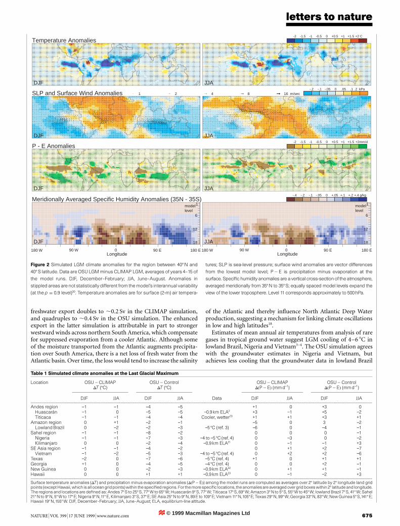
The cooler equatorial SSTs in the OSU simulation induce wide-spread atmospheric anomalies relative to the CLIMAP simulation(Fig. 2). Cooling is evident in summer (June, July, August; JJA) andwinter (December, January, February; DJF) over the central Andes,lowland South America, tropical and subtropical Africa, easternAfrica, the Arabian peninsula, and southern Asia. In the OSUsimulation, a large positive sea-level pressure anomaly associatedwith cooler SSTs spans the Equator in the tropical Atlantic andeastern Pacific oceans. The change in wind flow induced by thishigher pressure, and by opposing circulation patterns in the north-ern and southern hemispheres (clockwise and anticlockwise out ofhigh-pressure centres, respectively), is manifested in enhancedwestward flow over northern South America into the Pacific (JJA)and by enhanced eastward flow in the mid-latitudes over the SouthAtlantic (DJF and JJA). Elsewhere, modified pressure gradientschange surface winds over Africa, the Arabian peninsula, and theIndian Ocean. The monsoonal winds over India and southeast Asiaare weaker in the OSU simulation than in the control but strongerthan those of the CLIMAP simulation; they are thus more consistentwith an observed small reduction in Arabian Sea upwelling duringthe LGM15.

The equatorial Walker circulation is characterized as a zonalpattern of ascending air over Indonesia, South America, and Africaand descending air over the eastern Pacific, Atlantic and westernIndian oceans. Vertical motions are estimated here based on changesin the vertical pressure gradient in the model. Relative to CLIMAP,in the OSU simulation rising motions are weakened over SouthAmerica and strengthened over Indonesia, while sinking motionsare enhanced over the eastern Pacific, Atlantic, and western Indianoceans. Such changes, together with modified winds at the surfaceand aloft, indicate a stronger Walker circulation in the OSUsimulation, which contributes to changes in the distribution ofatmospheric moisture (Fig. 2).

In both seasons, net moisture (precipitation minus evaporation,P 2 E) anomalies are negative (that is, drier) in the OSU simulationrelative to CLIMAP near and just downwind of the cooler SSTs(Fig. 2). Seasonal drying in the OSU simulation extends well inlandover the Amazon basin and Central America. Drying also extendseastward over central Africa to the Indian Ocean. Off the Equator,the thermal gradients focus moisture from the relatively warmsubtropical gyres along the edges of the cool anomalies, resultingin net moisture increases over the Andes and northern Mexico,generally consistent with terrestrial data16. During boreal summer,in the OSU simulation wetter conditions also exist in the monsoonregions of India and southeast Asia, as a result of pressure-relatedchanges in wind fields and stronger rising and sinking motions inthe Indo-Pacific sector of the Walker circulation, however, both theOSU and CLIMAP simulations produce summer drying relative tothe control simulation.

Net export of atmospheric water vapour from the Atlanticdrainage helps to maintain modern global thermohaline oceancirculation. For the control simulation, our estimate of net fresh-water export from the Atlantic to the Pacific and Indian oceans(integrated vertically from 1,000 to 200 hPa) is ,0.1 Sv(1 Sv ¼ 106 m3 s 2 1), a value similar to other model estimates butlower than values inferred from atmospheric data17. In the model,

Figure 1 Sea surface temperature anomalies estimated from foraminiferal

species. a, CLIMAP LGM1 minus modern; b, OSU LGM7 minus modern. Points

indicate core locations of LGM samples. White areas indicate no data.

© 1999 Macmillan Magazines Ltd

letters to nature

NATURE | VOL 399 | 17 JUNE 1999 | www.nature.com 675

freshwater export doubles to ,0.2 Sv in the CLIMAP simulation,and quadruples to ,0.4 Sv in the OSU simulation. The enhancedexport in the latter simulation is attributable in part to strongerwestward winds across northern South America, which compensatefor suppressed evaporation from a cooler Atlantic. Although someof the moisture transported from the Atlantic augments precipita-tion over South America, there is a net loss of fresh water from theAtlantic basin. Over time, the loss would tend to increase the salinity

of the Atlantic and thereby influence North Atlantic Deep Waterproduction, suggesting a mechanism for linking climate oscillationsin low and high latitudes18.

Estimates of mean annual air temperatures from analysis of raregases in tropical ground water suggest LGM cooling of 4–6 8C inlowland Brazil, Nigeria and Vietnam3–4. The OSU simulation agreeswith the groundwater estimates in Nigeria and Vietnam, butachieves less cooling that the groundwater data in lowland Brazil

Temperature Anomalies

DJF

-2 -1.5 -1 -0.5 0 +0.5 +1 +1.5 +2 C

JJA

SLP and Surface Wind Anomalies

DJF

1 2 4 8 16 m/sec-.2 -.1 -.05 0 .05 .1 .2 kPa

JJA

P - E Anomalies

DJF

-2 -1.5 -1 -0.5 0 +0.5 +1 +1.5 +2mm/d

JJA

Meridionally Averaged Specific Humidity Anomalies (35N - 35S)

DJF

-.4 -.2 -.1 -.05 0 +.05 +.1 +.2 +.4 g/kg

JJA 18

1

12

6

modellevel

18

1

12

6

modellevel

180 W 90 W 0 90 E 180 ELongitude

180 W 90 W 0 90 E 180 ELongitude

Figure 2 Simulated LGM climate anomalies for the region between 408 N and

408 S latitude. Data are OSU LGM minus CLIMAP LGM, averages of years 4–15 of

the model runs. DJF, December–February; JJA, June–August. Anomalies in

stippled areas are not statistically different from the model’s interannual variability

(at the p ¼ 0:9 level)30. Temperature anomalies are for surface (2-m) air tempera-

tures; SLP is sea-level pressure; surface wind anomalies are vector differences

from the lowest model level; P 2 E is precipitation minus evaporation at the

surface. Specific humidity anomalies are a vertical cross-section of the atmosphere,

averaged meridionally from 358N to 358S; equally spaced model levels expand the

view of the lower troposphere. Level 11 corresponds approximately to 500hPa.

Table 1 Simulated climate anomalies at the Last Glacial Maximum

Location OSU 2 CLIMAPDT (8C)

OSU 2 ControlDT (8C)

OSU 2 CLIMAPDðP 2 EÞ (mmd−1)

OSU 2 ControlDðP 2 EÞ (mmd−1)

DJF JJA DJF JJA Data DJF JJA DJF JJA...................................................................................................................................................................................................................................................................................................................................................................

Andes region −1 −1 −4 −5 +1 0 +3 0Huascaran −1 0 −5 −5 −0.9 km ELA2 +3 −1 +5 −2Titicaca −1 −1 −4 −4 Cooler, wetter20 +1 +1 +3 +1

Amazon region 0 +1 −2 −1 −5 0 3 −2Lowland Brazil 0 −2 −2 −3 −5 8C (ref. 3) −6 0 −4 −1

Sahel region −1 −1 −8 −2 0 0 0 −1Nigeria −1 −1 −7 −3 −4 to −5 8C (ref. 4) 0 −3 0 −2Kilimanjaro 0 0 −2 −4 −0.9 km ELA21 0 −1 −1 +3

SE Asia region −1 −1 −4 −2 0 +1 +2 −7Vietnam −1 −2 −5 −3 −4 to −5 8C (ref. 4) 0 +2 +2 −6

Texas −2 0 −7 −6 −5 8C (ref. 4) +1 0 +1 +1Georgia +1 0 −4 −5 −4 8C (ref. 4) 0 0 +2 −1New Guinea 0 0 −2 −3 −0.9 km ELA22 0 +1 +1 −1Hawaii 0 0 +1 +1 −0.9 km ELA23 0 −1 −2 +3...................................................................................................................................................................................................................................................................................................................................................................Surface temperature anomalies (DT) and precipitation minus evaporation anomalies (DðP 2 EÞ) among the model runs are computed as averages over 28 latitude by 28 longitude land gridpoints (except Hawaii,which is all oceangridpoints)within the specified regions. For themore specific locations, the anomaliesare averagedovergridboxeswithin 28 latitudeand longitude.The regions and locations are defined as: Andes 78 S to 258 S, 778 W to 658 W; Huascaran 98 S, 778 W; Titicaca 178 S, 698 W; Amazon 38 N to 58 S, 558 W to 458 W; lowland Brazil 78 S, 418 W; Sahel218 N to 98 N, 58 W to 178 E; Nigeria 98 N,118 E, Kilimanjaro 38 S, 378 E; SE Asia 258 N to 98 N, 89E to 1098 E; Vietnam 118 N,1058 E; Texas 298 N, 998 W; Georgia 338 N, 838 W; New Guinea 58 S,1418 E;Hawaii 198 N,1558 W. DJF, December–February; JJA, June–August; ELA, equilibrium-line altitude.

© 1999 Macmillan Magazines Ltd

letters to nature

676 NATURE | VOL 399 | 17 JUNE 1999 | www.nature.com

(Table 1). In the Amazon lowlands the OSU simulation is substan-tially drier than the CLIMAP simulation (up to 5 mm d−1 in DJF),and is consistent with evidence for Pleistocene aridity19. Both theCLIMAP and OSU simulations are in agreement with groundwatertemperature estimates from Texas and Georgia4.

Glacier data from the Andes20, Kilimanjaro21, New Guinea22, andHawaii23 indicate that equilibrium-line altitudes were ,900 mlower than at present (,780 m reduction relative to lower sealevel). But limiting dates for these advances range widely (20–15 kyr ago for Huascaran, 30–10 kyr for Kilimanjaro, .15 kyr forNew Guinea and 22–9 kyr for Hawaii), so the synchronicity oflowered equilibrium-line altitudes across the tropics remains uncer-tain. For Kilimanjaro and Huascaran, the OSU simulation is 3–5 8Ccooler than the control, yielding approximate temperature-relateddepressions of equilibrium-line altitudes of 550–900 m (based on anominal tropical lapse rate of 5.5 8C km−1). In both areas netmoisture at the LGM is greater than that of the control, whichwould further enhance glacier growth. The OSU simulation is thusconsistent with regional glacier advances in the Andes and eastAfrica. We did not modify CLIMAP SSTs near New Guinea andHawaii, and as a result temperatures in the OSU simulation areessentially the same as those of the CLIMAP simulation (3 8C coolerand 1 8C warmer than the control, respectively) and perhapsinconsistent with local glaciation, indicating the need for furtherstudy of these regions24.

The OSU simulation helps to resolve some, but not all, disagree-ments between land and ocean data. We did not consider climatefeedbacks associated with LGM vegetation, and these may yieldfurther modelled cooling over land25. Although the ice-age tropicsin the OSU simulation are generally cooler and drier than thecontrol, some regions such as the Andean highlands are cooler andwetter, suggesting substantial variation within the tropics bothregionally and with altitude, consistent with recent datacompilations26. The LGM cooling in the OSU simulation agreeswell with recent ocean and atmosphere–ocean model simulationsover the eastern Pacific, the equatorial Atlantic and regions of Africaand Asia9,27–29. To the extent that our AGCM results are model-independent, this agreement suggests convergence of data andmodels in these regions. In the western Pacific, the OSU reconstructionagrees with one ocean simulation29 and one coupled atmosphere–ocean simulation28, but disagrees with a coupled atmosphere–oceansimulation that yields a cooling of 4–6 8C (ref. 27). Nevertheless, ourresults highlight the potentially widespread influences of regional SSTchanges in circulation patterns and moisture fluxes associated withtropical–extratropical temperature gradients, and understore theneed to reconstruct both the amplitude and the geographicaldistribution of LGM climate changes in much greater detail. M

Received 28 January; accepted 5 May 1999.

1. CLIMAP Project Members. Seasonal reconstruction of the earth’s surface at the last glacial maximum.(Map & Chart Ser. MC-3, Geol. Soc. Am., Boulder, Colorado, 1981).

2. Thompson, L. G. et al. Late glacial stage and Holocene tropical ice core records from Huascaran, Peru.Science 269, 46–50 (1995).

3. Stute, M. et al. Cooling of tropical Brazil (58 C) during the last glacial maximum. Science 269, 379–383(1995).

4. Stute, M. et al. Glacial paleotemperature records for the tropics derived from noble gases dissolved ingroundwater (abstr). Eos 78, F44 (1997).

5. Guilderson, T. P., Fairbanks, R. G. & Rubenstone, J. L. Tropical temperature variations since 20,000years ago: modulating interhemispheric climate change. Science 263, 663–665 (1994).

6. Rind, D. & Peteet, D. Terrestrial conditions at the last glacial maximum and CLIMAP sea-surfacetemperature estimates: are they consistent? Quat. Res. 24, 1–22 (1985).

7. Mix, A. C., Morey, A., Pisias, N. G. & Hostetler, S. Foraminiferal faunal estimates of paleotemperature:Circumventing the no-analog problem yields cool ice age tropics. Paleoceanography 14, 350–359 (1999).

8. Slowey, N. & Curry, W. B. Glacial-interglacial differences in circulation and carbon cycling within theupper western North Atlantic. Paleoceanography 10, 715–732 (1995).

9. Ganopolski, A., Rahmstorf, S., Petoukhov, V. & Claussen, M. Simulation of modern and glacialclimates with a coupled global model of intermediate complexity. Nature 391, 351–356 (1998).

10. Thompson, S. L. & Pollard, D. A global climate model (GENESIS) with a land-surface-transfer scheme(LSX), 1, present-day climate. J. Clim. 8, 732–761 (1995).

11. Dorman, J. L. & Sellers, P. J. A global climatology of albedo, roughness length, and stomatal resistancefor atmospheric general circulation models as represented by the simple biosphere model (SiB). J.Appl. Meteorol. 28, 833–855 (1989).

12. Clark, P. U., Licciardi, J. M., MacAyeal, D. R. & Jenson, J. W. Numerical reconstruction of a soft-bedded Laurentide ice sheet during the last glacial maximum. Geology 24, 679–682 (1996).

13. Peltier, W. R. Ice age paleotopography. Science 265, 195–201 (1994).14. Thunell, R. C., Anderson, D. M., Gellar, D. & Miao, Q. Sea-surface temperature estimates for the

tropical western Pacific during the last glaciation and their implications for the Pacific warm pool.Quat. Res. 41, 255–264 (1994).

15. Prell, W. L. & Kutzbach, J. E. Monsoon variability over the past 150,000 years. J. Geophys. Res. 92,8411–8425 (1987).

16. Markgraf, V. in Global Climates Since the Last Glacial Maximum (eds Wright, H. E. et al.) 357–385(Univ. Minnesota Press, Minneapolis, 1993).

17. Zaucker, F. & Broecker, W. S. The influence of atmospheric moisture transport on the fresh waterbalance of the Atlantic drainage basin: General circulation model simulations and observations. J.Geophys. Res. 97, 2765–2773 (1992).

18. Zaucker, F., Stocker, T. F. & Broecker, W. S. Atmospheric freshwater fluxes and their effect on the globalthermohaline circulation. J. Geophys. Res. 99, 12443–12457 (1994).

19. Servant, M. et al. Tropical forest changes during the late Quaternary in African and South Americanlowlands. Glob. Planet. Change 7, 25–40 (1993).

20. Klein, A. G., Seltzer, G. O. & Isacks, B. L. Modern and last local glacial maximum snowlines in theCentral Andes of Peru, Bolivia, and Northern Chile. Quat. Sci. Rev. 18, 63–84 (1999).

21. Downie, C. & Wilkinson, P. The Geology of Kilimanjaro (Univ. Sheffield Press, 1972).22. Loffler, E. Pleistocene glaciation in Papua and New Guinea. Z. Geomorphol. 13, 32–58 (1972).23. Porter, S. C. Chronology of Hawaiian glaciations. Science 195, 61–63 (1977).24. Lee, K. E. & Slowey, N. C. Cool surface waters of the subtropical North Pacific Ocean during the last

glacial. Nature 397, 512–514 (1999).25. Crowley, T. J. & Baum, S. K. Effect of vegetation on an ice-age climate model simulation. J. Geophys.

Res. 102, 16463–16480 (1997).26. Farrera, I. et al. Tropical climates at the last glacial maximum: A new synthesis of terrestrial

palaeoclimate data, I, Vegetation, lake levels, and geochemistry. Clim. Dyn. (in the press).27. Bush, A. B. G. & Philander, S. G. H. The role of ocean-atmosphere interactions in tropical cooling

during the last glacial maximum. Science 279, 1341–1344 (1998).28. Weaver, A. J., Eby, M., Fanning, A. F. & Wiebe, E. C. Simulated influence of carbon dioxide, orbital

forcing, and ice sheets on the climate of the last glacial maximum. Nature 394, 847–853 (1998).29. Bigg, G. R., Wadley, M. R., Stevens, D. P. & Johnson, J. A. Simulation of two last glacial maximum

ocean states. Paleoceanography 13, 340–351 (1998).30. Chervin, R. M. Interannual variability and seasonal predictability. J. Atmos. Sci. 43, 233–241 (1986).

Acknowledgements. We thank P. Bartlein for discussions and the design of Fig. 2; P. Clark, N. Pisias,D. Pollard for discussions; P. Valdez for comments and suggestions; and A. Morey and D. Zahnle forassistance. Model simulations were conducted at the National Center for Atmospheric Research, theEnvironmental Protection Agency, and the College of Oceanic and Atmospheric Sciences at Oregon StateUniversity. The US Geological Survey (S.W.H.) and The National Science Foundation (A.C.M.)supported this research.

Correspondence and requests for materials should be addressed to S.W.H. (e-mail: steve@ucar.edu).

Goldconcentrationsofmagmatic brinesandthemetal budget ofporphyrycopperdepositsT. Ulrich*, D. Gunther*† & C. A. Heinrich*

* Isotope Geology and Mineral Resources, Department of Earth Sciences,ETH Zentrum 8092 Zurich, Switzerland. . . . . . . . . . . . . . . . . . . . . . . . . . . . . . . . . . . . . . . . . . . . . . . . . . . . . . . . . . . . . . . . . . . . . . . . . . . . . . . . . . . . . . . . . . . . . . . . . . . . . . . . . . . . . . . . . . . . . . . . .

Porphyry copper–molybdenum–gold deposits are the mostimportant metal resources formed by hydrothermal processesassociated with magmatism. It remains controversial, however,whether the metal content of porphyry-style and other mag-matic–hydrothermal deposits is dominantly controlled by metalpartitioning between magma and an exsolving magmatic fluidphase1,2 or by scavenging of metals from solid upper-crustal rocksby surface-derived fluids3. It also remains unknown to whatdegree the metal content in such deposits is affected by selectivemineral precipitation from the ore fluid. Extremely saline fluids4,precipitating quartz and ore minerals in veins have been inferredto have a significant magma-derived component, on the basis ofgeological5, isotopic6,7 and experimental evidence8,9. Here wereport gold and copper concentrations of single fluid inclusionsin quartz, determined by laser-ablation inductively coupledplasma mass spectrometry. The results show that the Au/Curatio of primary high-temperature brines is identical to the bulkAu/Cu ratio in two of the world’s largest copper–gold ore bodies.This indicates that the bulk metal budget of such deposits isprimarily controlled by the composition of the incoming fluid,which is, in turn, likely to be controlled by the crystallization

† Present address: Laboratory of Inorganic Chemistry, ETH Zentrum 8092 Zurich, Switzerland.