Reassessing False Discoveries in

Mutual Fund Performance: Skill,

Luck, or Lack of Power?

A Reply

LAURENT BARRAS, OLIVIER SCAILLET, and RUSS WERMERS∗

ABSTRACT

Andrikogiannopoulou and Papakonstantinou (2019, AP) inquire into

the bias of the False Discovery Rate (FDR) estimators of Barras,

Scaillet, and Wermers (2010, BSW). In this Reply, we replicate their

results, then explore the bias issue further by (i) using different pa-

rameter values and (ii) updating the sample period. Over the original

period (1975 to 2006), we show that reasonable adjustments to the pa-

rameter choices made by BSW and AP result in a sizeable reduction

in the bias relative to AP. Over the updated period (1975 to 2018), we

∗Barras (corresponding author, laurent.barras@mcgill.ca) is at McGill University (De-sautels Faculty of Management), Scaillet is at the University of Geneva (Geneva FinanceResearch Institute (GFRI)) and at the Swiss Finance Institute (SFI), and Wermers isat the University of Maryland (Smith School of Business). We thank the Editor, StefanNagel, and two anonymous referees for very helpful feedback. We have read the Journalof Finance’s disclosure policy and have no conflicts of interest to disclose.

1

show that the performance of the FDR improves dramatically across

a large range of parameter values. Specifically, we find that the proba-

bility of misclassifying a fund with a true alpha of 2% per year is 32%

(versus 65% in AP). Our results, together with those of AP, indicate

that the use of the FDR in finance should be accompanied by a careful

evaluation of the underlying data-generating process, especially when

the sample size is small.

In a paper published in the Journal of Finance, Barras, Scaillet, and Wer-

mers (2010, henceforth BSW) apply a new econometric approach—the False

Discovery Rate (FDR)—to the field of mutual fund performance. BSW use

this approach with two main objectives in mind: (i) estimate the propor-

tions of zero and nonzero alpha funds in the population, π0 and πA, and

(ii) form portfolios of funds that differ in their ability to generate future

(out-of-sample) positive alphas.1

It is well known from theory that the FDR estimators, π̂0 and π̂A, are

potentially biased, as π̂0 overestimates π0 and π̂A underestimates πA (e.g.,

Genovese and Wasserman (2004), Storey (2002)). This issue arises when

nonzero alpha funds are difficult to detect in the data, because their alphas

are small, estimation noise is large, or both. Whereas using a conservative

estimator, π̂0, is beneficial for the selection of a subset of truly outperforming

funds (objective (ii) of BSW), it may result in an undesirable level of bias in

evaluating performance in the overall fund population (objective (i) of BSW).

To quantify this bias, BSW perform simulation analysis and conclude that

1Henceforth, “zero alpha funds” (“nonzero alpha funds”) refers to those funds that

have a true model alpha equal to zero (different from zero).

2

both π̂0 and π̂A are close to their true values.

Andrikogiannopoulou and Papakonstantinou (2019, henceforth AP) chal-

lenge the simulation analysis of BSW based on the choice of parameter values.

First, AP correctly point out that BSW set the number of assumed fund re-

turn observations too high, which artificially reduces the estimation noise

compared to the actual sample. Second, AP consider smaller (in magni-

tude) values for the true alphas of nonzero alpha funds. Incorporating these

changes, AP conclude from simulations based on revised parameter values

that the proportions π̂0 and π̂A are heavily biased. AP, therefore, question

the usefulness of the FDR approach for evaluating the performance of mutual

funds (objective (i) of BSW).

AP conduct an important critical evaluation of the FDR approach for

the benefit of empirical research. The FDR has been increasingly used as an

estimation approach to evaluate mutual fund performance, as well as being

used in other areas of finance, because it is simple and fast—simply put, it

amounts to estimating a simple average based on t-statistics.2 This contrasts

with alternative approaches that impose much more structure to improve esti-

mation performance. Bayesian/parametric approaches, for instance, require

computer-intensive numerical estimation of π0 and πA using sophisticated

Markov Chain Monte Carlo (MCMC) and Expectation-Maximization (EM)

methods. Thus, if the FDR approach is to be discarded, the costs to re-

2See, among others, Augustin, Brenner, and Subrahmanyam (2019), Bajgrowicz and

Scaillet (2012), Barras (2019), Cuthbertson, Nitzsche, and O’Sullivan (2008), Ferson and

Chen (2020), Giglio, Liao, and Xiu (2019), and Scaillet, Treccani, and Trevisan (forth-

coming).

3

searchers in terms of time and complexity are potentially large.3

In this Reply to AP, we further assess the bias of the FDR estimators.

We begin by replicating the results of BSW and AP. We, then, extend the

BSW and AP simulation results by (i) using parameter values that we believe

better reflect the data-generating process (DGP) of mutual fund alphas in the

real world, and (ii) updating the sample period. In doing so, we develop an

analytical approach that allows us to quantify the bias of the FDR estimator

without recourse to simulations.4 The analytical approach is simple and

allows for a completely transparent comparison of the results in BSW, AP,

and our Reply.

Our results reveal that the changes in parameter values materially affect

the evaluation of the FDR approach. Over the original period (1975 to

2006), we find that the bias decreases significantly relative to AP after (i)

considering alternative values for the residual volatility of individual funds

and (ii) accounting for the relations between the different parameters that

are motivated by theory and supported by empirical evidence. To illustrate,

3If the FDR is discarded, researchers also lose the benefits of the FDR as a nonpara-

metric approach. Specifically, the FDR makes no assumptions about the shape of the

alpha distributions of negative versus positive alpha funds. Therefore, it is less susceptible

to potential misspecification errors that arise when researchers make incorrect specification

assumptions about the shape of these distributions.

4To explain, we build on the analysis of BSW and AP, making the same assumptions

regarding the DGP for the cross-section of mutual fund returns. Given these assumptions,

we show that a simulation analysis is unnecessary—instead, we use the properties of

the Student t-distribution to derive exact expressions for the probability that the FDR

misclassifies nonzero alpha funds, and the bias of the FDR proportions π̂0 and π̂A.

4

while AP find that a fund with a true alpha of 2% per year is misclassified

as a zero alpha fund 65% of the time, we find that the misclassification

probability is equal to 44%. The evidence documented here, therefore, is

more nuanced than in BSW and AP. In particular, whereas we confirm that

the initial analysis of BSW may be too optimistic, we do not find the high

levels of bias documented by AP.

Next, we provide updated evidence on the bias by examining the period

1975 to 2018 (by contrast, BSW and AP study the period 1975 to 2006). Over

this extended period, the performance of the FDR improves significantly,

regardless of the procedure employed to choose the parameter values. Using

the same procedure as in BSW and AP, we find that the probability of

misclassifying a fund with an alpha of 2% per year drops to 37%. Using

the procedure proposed here, the misclassification probability drops further

to 32%. We, therefore, believe that the FDR approach does a good job

capturing the salient features of the cross-sectional alpha distribution.

Our Reply has implications beyond the context of evaluating mutual fund

performance. First, it highlights the importance of carefully analyzing the

properties of the data to assess the benefits of the FDR. Such analysis is

particularly important if the sample period is relatively short. Second, it

provides a simple approach for evaluating the bias of the FDR without re-

course to simulations—a practical benefit to empiricists who wish to explore

the performance of the FDR approach for their empirical application.

The remainder of our Reply is organized as follows. Section I provides

background on the context behind the critique of AP. Section II describes our

new methodology for computing the bias of the FDR proportions. Section III

5

replicates the results of BSW and AP. Section IV presents our analysis and

summarizes our main findings. The Appendix provides additional details on

our new methodology.

I. The Context

To place our Reply to AP in context, we first discuss the applications

of the FDR approach to mutual fund performance as specified in BSW, in-

cluding the procedure for estimating the FDR proportions of zero alpha and

nonzero alpha funds. We then review the bias of the FDR proportions.

A. The FDR Approach

A.1. Applications of the FDR Approach

As explained in their introduction (p. 180), BSW apply the FDR ap-

proach to a large panel of mutual funds to (i) estimate the proportions of

zero alpha and nonzero alpha funds, π0 and πA, and (ii) based on these pro-

portion estimates, select subgroups of funds to determine whether mutual

fund performance persists out of sample.5

To meet the first objective, BSW use the FDR as an estimation approach.

This approach proposed by Storey (2002) is straightforward—it uses as inputs

5In the first paragraph of the introduction, BSW summarize these two objectives as

follows: “... It is natural to wonder how many fund managers possess true stockpicking

skills, and where these funds are located in the cross-sectional estimated alpha distribution.

From an investment perspective, precisely locating skilled funds maximizes our chances of

achieving persistent outperformance” (p. 180).

6

only the p-values of the fund alphas obtained from a regression of individual

fund returns on benchmark returns. Whereas the p-values of nonzero alpha

funds are typically close to zero because their alphas are different from zero,

the p-values of zero alpha funds generally take large values. By choosing a

small interval, Ip, close to one, we can bifurcate the two categories of funds—

zero and nonzero alpha funds—and estimate the FDR proportions π0 and πA

(see Figure 2 of BSW, p. 188, for a graphical illustration).

To meet the second objective, BSW use the FDR as a multiple testing

approach. The basic idea is to conduct a test of the null hypothesis for each

fund i, H0,i: αi = 0 (for i = 1, 2, ...), to select funds with positive alphas.

When conducting this multiple testing approach on several thousand funds,

we are likely to have many false discoveries—true zero alpha funds that, by

chance, exhibit nonzero estimated alphas of a significant magnitude. Using

the FDR allows us to explicitly control for these false discoveries. In other

words, it is an extension of the notion of Type I error from single to multiple

hypothesis testing.

The critique of AP pertains to the first objective of BSW. Accordingly,

we focus below exclusively on the properties of the FDR proportions. We

refer the reader interested in multiple testing (including its application to

finance) to the extensive literature devoted to this issue (see, among others,

Bajgrowicz and Scaillet (2012), Bajgrowicz, Scaillet, and Treccani (2016),

BSW, Benjamini and Hochberg (1995), Efron (2010), and Storey (2002)).

7

A.2. The FDR Proportions

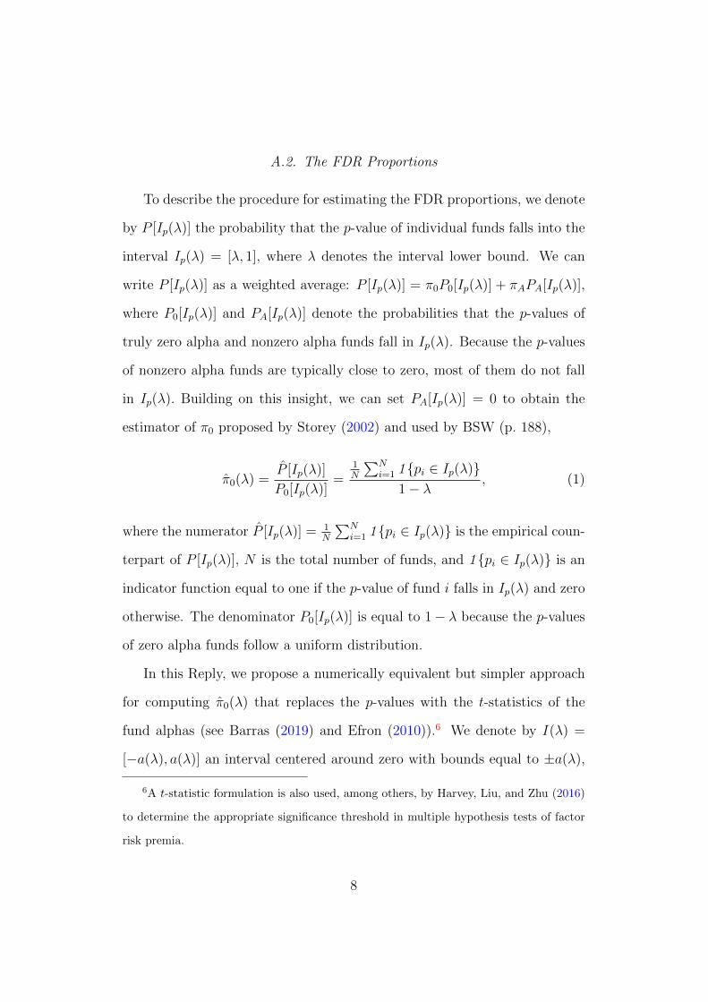
To describe the procedure for estimating the FDR proportions, we denote

by P [Ip(λ)] the probability that the p-value of individual funds falls into the

interval Ip(λ) = [λ, 1], where λ denotes the interval lower bound. We can

write P [Ip(λ)] as a weighted average: P [Ip(λ)] = π0P0[Ip(λ)] + πAPA[Ip(λ)],

where P0[Ip(λ)] and PA[Ip(λ)] denote the probabilities that the p-values of

truly zero alpha and nonzero alpha funds fall in Ip(λ). Because the p-values

of nonzero alpha funds are typically close to zero, most of them do not fall

in Ip(λ). Building on this insight, we can set PA[Ip(λ)] = 0 to obtain the

estimator of π0 proposed by Storey (2002) and used by BSW (p. 188),

π̂0(λ) =P̂ [Ip(λ)]

P0[Ip(λ)]=

1N

∑Ni=1 1{pi ∈ Ip(λ)}

1− λ, (1)

where the numerator P̂ [Ip(λ)] = 1N

∑Ni=1 1{pi ∈ Ip(λ)} is the empirical coun-

terpart of P [Ip(λ)], N is the total number of funds, and 1{pi ∈ Ip(λ)} is an

indicator function equal to one if the p-value of fund i falls in Ip(λ) and zero

otherwise. The denominator P0[Ip(λ)] is equal to 1− λ because the p-values

of zero alpha funds follow a uniform distribution.

In this Reply, we propose a numerically equivalent but simpler approach

for computing π̂0(λ) that replaces the p-values with the t-statistics of the

fund alphas (see Barras (2019) and Efron (2010)).6 We denote by I(λ) =

[−a(λ), a(λ)] an interval centered around zero with bounds equal to ±a(λ),

6A t-statistic formulation is also used, among others, by Harvey, Liu, and Zhu (2016)

to determine the appropriate significance threshold in multiple hypothesis tests of factor

risk premia.

8

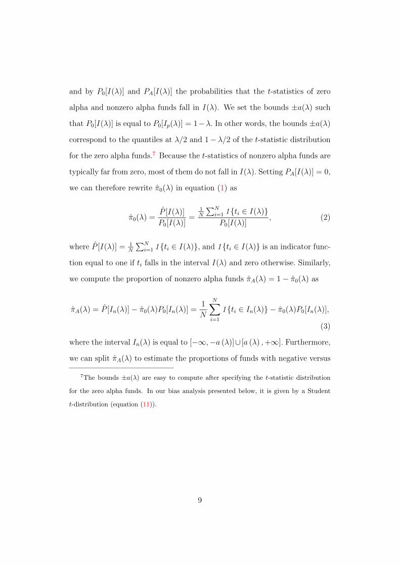
and by P0[I(λ)] and PA[I(λ)] the probabilities that the t-statistics of zero

alpha and nonzero alpha funds fall in I(λ). We set the bounds ±a(λ) such

that P0[I(λ)] is equal to P0[Ip(λ)] = 1−λ. In other words, the bounds ±a(λ)

correspond to the quantiles at λ/2 and 1− λ/2 of the t-statistic distribution

for the zero alpha funds.7 Because the t-statistics of nonzero alpha funds are

typically far from zero, most of them do not fall in I(λ). Setting PA[I(λ)] = 0,

we can therefore rewrite π̂0(λ) in equation (1) as

π̂0(λ) =P̂ [I(λ)]

P0[I(λ)]=

1N

∑Ni=1 1{ti ∈ I(λ)}P0[I(λ)]

, (2)

where P̂ [I(λ)] = 1N

∑Ni=1 1{ti ∈ I(λ)}, and 1{ti ∈ I(λ)} is an indicator func-

tion equal to one if ti falls in the interval I(λ) and zero otherwise. Similarly,

we compute the proportion of nonzero alpha funds π̂A(λ) = 1− π̂0(λ) as

π̂A(λ) = P̂ [In(λ)]− π̂0(λ)P0[In(λ)] =1

N

N∑i=1

1{ti ∈ In(λ)} − π̂0(λ)P0[In(λ)],

(3)

where the interval In(λ) is equal to [−∞,−a (λ)]∪ [a (λ) ,+∞]. Furthermore,

we can split π̂A(λ) to estimate the proportions of funds with negative versus

7The bounds ±a(λ) are easy to compute after specifying the t-statistic distribution

for the zero alpha funds. In our bias analysis presented below, it is given by a Student

t-distribution (equation (11)).

9

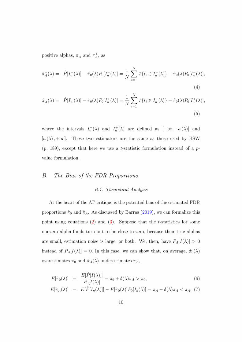
positive alphas, π−A and π+A , as

π̂−A(λ) = P̂ [I−n (λ)]− π̂0(λ)P0[I−n (λ)] =

1

N

N∑i=1

1{ti ∈ I−n (λ)} − π̂0(λ)P0[I−n (λ)],

(4)

π̂+A(λ) = P̂ [I+n (λ)]− π̂0(λ)P0[I

+n (λ)] =

1

N

N∑i=1

1{ti ∈ I+n (λ)} − π̂0(λ)P0[I+n (λ)],

(5)

where the intervals I−n (λ) and I+n (λ) are defined as [−∞,−a (λ)] and

[a (λ) ,+∞]. These two estimators are the same as those used by BSW

(p. 189), except that here we use a t-statistic formulation instead of a p-

value formulation.

B. The Bias of the FDR Proportions

B.1. Theoretical Analysis

At the heart of the AP critique is the potential bias of the estimated FDR

proportions π̂0 and π̂A. As discussed by Barras (2019), we can formalize this

point using equations (2) and (3). Suppose that the t-statistics for some

nonzero alpha funds turn out to be close to zero, because their true alphas

are small, estimation noise is large, or both. We, then, have PA[I(λ)] > 0

instead of PA[I(λ)] = 0. In this case, we can show that, on average, π̂0(λ)

overestimates π0 and π̂A(λ) underestimates πA,

E[π̂0(λ)] =E[P̂ [I(λ)]]

P0[I(λ)]= π0 + δ(λ)πA > π0, (6)

E[π̂A(λ)] = E[P̂ [In(λ)]]− E[π̂0(λ)]P0[In(λ)] = πA − δ(λ)πA < πA, (7)

10

where we define the ratio δ(λ) as

δ(λ) =PA[I(λ)]

P0[I(λ)]=PA[I(λ)]

1− λ. (8)

Taking the expectations of equations (4) and (5), we can further show that

π̂−A(λ) and π̂+A(λ) are also biased (see the Appendix).

We can write the ratio δ(λ) as the relative bias of π̂A(λ), that is,

δ(λ) =πA − E[π̂A(λ)]

πA. (9)

Equation (9) implies that we can interpret δ(λ) as the misclassification prob-

ability associated with the FDR approach. For instance, a value of 40%

for δ(λ) implies a 40% probability that nonzero alpha funds are incorrectly

classified as zero alpha funds. Because δ(λ) is a relative measure, we can

compute it without having to specify the true proportions π0, π−A , and π+

A .

For this reason, δ(λ) provides a convenient measure of the bias implied by

the FDR approach.

The potential bias of the estimated FDR proportions has been known

for some time—it is discussed extensively in the statistical papers cited by

BSW (Genovese and Wasserman (2004), Storey (2002), Storey, Taylor, and

Siegmund (2004)). In addition, several finance papers explicitly discuss the

potential bias of the FDR proportions and propose alternative approaches

that impose more parametric assumptions on the fund alpha distribution

(e.g., Chen, Cliff, and Zhao (2017), Ferson and Chen (2020), Harvey and

11

Liu (2018) ).8 However, these papers provide limited information on the

magnitude of the bias in the context of mutual funds.9

B.2. Quantitative Analysis

Two studies provide a quantitative assessment of the bias of the FDR

proportions. BSW perform a simulation analysis calibrated on the data over

the period 1975 to 2006. The results reported in the Internet Appendix of

BSW reveal that both the bias and the variance of π̂0(λ) and π̂A(λ) are small:

“...the simulation results reveal that the average values of our estimators

closely match the true values, and that their 90% confidence intervals are

narrow” (p. 5 of the Internet Appendix).

More recently, AP perform simulation analysis using the same 1975 to

2006 period, but they consider scenarios in which funds have different as-

sumed alphas and/or shorter return time-series than those examined in BSW.

Contrary to BSW, AP find that π̂0(λ) and π̂A(λ) are heavily biased. Moti-

vated by these results, AP question the applicability of the FDR approach

for evaluating mutual fund performance: “Overall, our results raise con-

cerns about the applicability of the FDR in fund performance evaluation

8If these specification assumptions are correct, the proposed estimators achieve better

performance than the FDR estimators. However, if they are incorrect, the proposed

estimators are plagued by misspecification errors and could potentially be more biased

than the FDR estimators.

9One exception is Ferson and Chen (2020) who perform simulation analysis to examine

the properties of the FDR estimators. However, the results are difficult to compare with

those in BSW and AP, because the simulations are calibrated on hedge fund data.

12

and more widely in finance where the signal-to-noise ratio in the data is

similarly low”(p. 2).

These two studies reach different conclusions regarding the bias of the

FDR proportions. To understand the reasons for these large differences,

we propose a novel methodology that allows for a simple and transparent

analysis of the bias.

II. Methodology for Computing the Bias

In presenting our methodology, we first discuss the main distributional

assumptions that we make on mutual fund returns. Building on these as-

sumptions, we then propose a simple analytical approach to compute the

bias without recourse to simulations.

A. Mutual Fund Returns

To specify the time-series properties of fund returns, we use the same

DGP as that proposed by BSW (p. 3 of the Internet Appendix), and used

by both BSW and AP. Our analysis, therefore, guarantees a fair comparison

between the results documented in (i) BSW, (ii) AP, and (iii) our Reply.

We assume that the excess net return ri,t of each fund i (i = 1, ..., N)

during each month t (t = 1, ..., T ) can be written as

ri,t = αi + birm,t + sirsmb,t + hirhml,t +mirmom,t + εi,t = αi + β′ift + ei,t, (10)

where αi is the net alpha, ft = (rm,t, rsmb,t, rhml,t, rmom,t)′ is the vector of

13

benchmark excess returns for market, size, value, and momentum, βi =

(bi, si, hi,mi)′ is the vector of fund betas, and ei,t is the error term (un-

correlated across funds). We also assume that ft and ei,t are independent

and normally distributed: ft ∼ N(0, Vf ), ei,t ∼ N(0, σ2e), where Vf is the

factor covariance matrix and σ2e denotes the residual variance.

Under these assumptions, the t-statistic ti follows a Student t-distribution

(tc) with T − 5 degrees of freedom if the fund alpha is null:

ti ∼ tc(T ), if αi = 0. (11)

If the fund alpha is different from zero, ti follows a noncentral Student t-

distribution (tnc) with T−5 degrees of freedom and a noncentrality parameter

t̄ equal to ασe/√T

:

ti ∼ tnc(α, σe, T ), if αi = α 6= 0. (12)

These distributional results are exact (i.e., they hold for fixed T ) because the

error term is independent, identically normally distributed, and orthogonal

to the factors.

B. A Simple Analytical Approach

BSW and AP estimate the bias of π̂0(λ) and π̂A(λ) via a simulation ap-

proach that requires that all of the parameters in equation (10) be specified.

However, this approach is unnecessary given the assumptions above. In par-

ticular, we can instead use an analytical approach that delivers exact values

for the bias directly from the Student t-distributions.

14

Using an analytical approach is simpler and faster. For one, it only re-

quires that we specify the three parameters of the Student t-distributions

(i.e., α, σe, and T ). Moreover, it is immune to simulation noise by construc-

tion. Finally, it allows for a completely transparent analysis of the bias—

conditional on the choice of parameters, there is only one possible output.

In our Reply, therefore, we use this analytical approach to study the bias of

the FDR proportions.

The main computation step is to quantify the misclassification probability

in equation (8). After specifying the values for α, σe, and T, we compute

δ(λ) as

δ(λ) =Fnc(I(λ);α, σe, T )

1− λ, (13)

where Fnc(I(λ);α, σe, T ) is the probability inferred from the noncentral Stu-

dent distribution tnc over the interval I(λ) = [−a(λ), a(λ)], where the bounds

±a(λ) correspond to the quantiles at λ/2 and 1−λ/2 of the central Student

distribution tc. We can then substitute δ(λ) into equations (6) and (7) to

obtain the (absolute) bias of π̂0(λ) and π̂A(λ). As discussed in the Appendix

of this Reply, we can also use δ(λ) to compute the (absolute) bias of the

proportions of negative versus positive alpha funds, π̂−A(λ) and π̂+A(λ).

III. Replication Analysis

We begin our analysis by replicating the results of BSW and AP using

the analytical approach presented above. The objectives of this replication

analysis are twofold. First, it confirms that the analytical approach yields

similar results as those obtained via simulation (as expected from econometric

15

theory). Second, it allows us to discuss the choice of parameter values in BSW

and AP, as well as its impact on the bias of the FDR proportions.

A. The Results in BSW

BSW calibrate their simulations using a sample of all active U.S. equity

funds (2,076 funds with a minimum of 60 monthly observations) over the

period January 1975 to December 2006 (“original sample” henceforth). They

set σe equal to the empirical mean of the residual volatility across funds, and

T equal to the total sample size: σe = 0.021, T = 384.10 Using a calibration

based on the FDR approach, they further specify that negative alpha funds

exhibit an alpha of -3.2% per year, whereas positive alpha funds earn an

alpha of 3.8% per year—α−ann = −3.2%, α+ann = 3.8%—where α−ann and α+

ann

are divided by 12 to obtain monthly values. Finally, they use the estimated

FDR proportions as proxies of the true proportions: π0 = 75%, π−A = 23%,

π+A = 2%. Additional details on the calibration can be found in the Internet

Appendix of BSW (pp. 3–7).

To compute the misclassification probability and the bias terms, we must

specify the interval I(λ) by choosing the parameter value λ. For simplicity, we

initially set λ equal to 0.5—this value is viewed as reasonable by BSW (p. 8

of the Internet Appendix), and is used by AP in some of their calculations

(see their Figure 1). We discuss alternative values for λ in Section IV.A

10To be more precise, the empirical mean across all funds is equal to 0.020 (and not

0.021). BSW use a value of 0.021 because they work with a randomly selected subsample

of 1,400 (out of the 2,076) funds that allow them to compare results with and without

cross-fund dependence.

16

below.

Table I reports results of our replication exercise. Panel A shows the

misclassification probability δ(λ) for the two values of the true alpha, that

is, |αann| = {3.2%, 3.8%}. In both cases, the probability of misclassifying

nonzero alpha funds is close to zero. Consistent with these results, Panel

B shows that the bias levels for π̂0(λ), π̂−A(λ), and π̂+A(λ) are all very small

(below 2%). Therefore, our computations closely replicate the results docu-

mented by BSW in their Table IA.I (p. 20 of the Internet Appendix).

Please insert Table I here

B. The Results in AP

Next, we repeat our replication exercise for AP, who use a similar sample

as BSW (active U.S. equity funds between January 1975 and December 2006).

AP improve the initial analysis of BSW along two dimensions. First, they

point out that using T = 384 overestimates the typical time-series length of

mutual fund returns. Using the empirical average of the number of monthly

observations across funds, AP set T equal to 150 (σe = 0.021, T = 150).

Second, they note that the simulation analysis of BSW is incomplete because

it examines only two values of alpha. To address this issue, they consider

a wider range of values for negative versus positive alpha funds, that is,

α−ann = −αann and α+ann = αann, where αann = {1.0%, 1.5%, ..., 3.5%}.

AP consider four values for the proportion vector (π0, π−A , π

+A)′. Specifi-

cally, they choose four values for π0: 94%, 75.0%, 38%, and 6%. For each

value of π0, they determine π−A and π+A such that the ratio π−A/π

+A remains

17

equal to 11.5 as in BSW (i.e., 23/2 = 11.5).

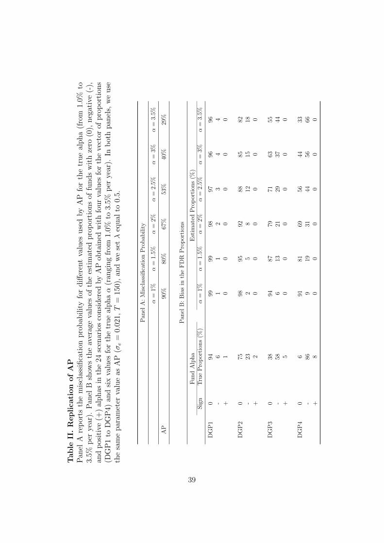
Panel A of Table II reports the misclassification probability δ(λ) for each

value of the true alpha αann. Panel B reports the bias of the FDR proportions

across the 24 scenarios (four proportion vectors × six alphas). We find that

our analytical approach closely replicates the results obtained by AP. In

particular, we find that 67% of the funds with an alpha of 2% per year are

misclassified as zero alpha funds—a number close to that reported by AP

in their abstract: “65% of funds with economically large alphas of ±2% are

misclassified as zero alpha.” In addition, the differences in bias for π̂0(λ)

relative to the results in Table V of AP are equal, on average, to only 0.5%

across all scenarios.11

Overall, the replication results confirm the analysis of AP. If we change

the initial framework of BSW by (i) decreasing the number of observations

and (ii) reducing the alpha that funds may exhibit, the FDR proportions

become markedly biased.

Please insert Table II here

11The tiny observed differences are due to several factors. First, AP only set λ equal

to 0.5 to plot their Figure 1. For the simulations, they follow BSW and use the Mean

Squared Error (MSE)-minimization procedure of Storey (2002) to select λ across values

ranging from 0.3 to 0.7. Second, AP do not set T = 150 for all funds, but randomly

draw values from the empirical distribution in their sample, which has a median of 150.

Third, AP set the mean of ft equal to its empirical average (instead of zero). Finally, the

simulation analysis does not yield exact values because it is subject to simulation noise.

18

IV. Our Analysis

We now turn to the main analysis of our Reply. In Section IV.A, we

revisit the analysis of BSW and AP by considering alternative values for the

parameters and for the interval I(λ). In Section IV.B, we update the evidence

on the bias by extending the sample period from 2006 to 2018. Section IV.C

summarizes our results.

A. Criticism of BSW and AP

A.1. The Choice of Parameter Values

We agree with AP that the initial analysis of BSW overestimates the

number of observations T and focuses on somewhat limited values of the

true alpha of nonzero alpha funds. In addition to these modifications, we

argue that two additional changes in parameter values are important to re-

produce the salient feature of mutual fund data. These changes, which are

not considered by BSW and AP, could materially affect the performance of

the FDR estimators.

(i) Residual volatility. Throughout their analyses, BSW and AP set the

residual volatility equal to the empirical mean across funds (σe = 0.021). This

value is then used as a proxy for the residual volatility of all funds in the

population. The main issue with this approach is that the mean is influenced

by a few extremely volatile funds. That is, the cross-sectional distribution of

residual volatility is heavily skewed (the skewness is equal to 3.9). To obtain

a value for σe that is more representative of the typical fund, we propose a

19

simple solution—replacing the mean with the median. Applying this change

to both the residual volatility and the number of observations, we obtain

σe = 0.018 and T = 135.12

(ii) Relations between fund parameters. AP extend the analysis of BSW

by considering a large set of values for the true alpha αann. Specifically, they

examine different scenarios in which αann varies but the other parameters σe

and T stay constant. As theory suggests, however, these scenarios may not be

realistic representations of the real world. If a fund has a high alpha and low

residual volatility, it will be highly attractive because of its high information

ratio (Treynor and Black (1973)). Stambaugh (2014) shows that as investors

allocate more money to such a fund, capacity constraints will tighten and its

alpha will move downward in line with its residual volatility (i.e., lower σe

means lower α).13 Furthermore, the model of Berk and Green (2004) implies

that funds deliver positive alphas only during the learning phase when they

are young (i.e., higher T means lower α). These arguments suggest that an

analysis in which α varies should allow for the possibility that σe and T vary

as well.

We propose a simple calibration approach to capture the relations be-

tween parameters. For each value of αann, we select a total of Jα funds

whose estimated alpha α̂ann falls in the bin αann±0.5%, where the bin width

12For consistency, we also use the median for the number of return observations (T =

135). Choosing T = 150 as in AP would therefore improve the accuracy of the FDR

estimators reported in Table IV.

13In the model of Stambaugh (2014), there is a one-to-one mapping between α and σe

because the information ratios of all funds must be equal in equilibrium.

20

corresponds to the distance between the different values of αann examined

by AP (αann = {1.0%, 1.5%, ..., 3.5%}). Extending equation (13), we then

compute the misclassification probability δ(λ) by using the values of σej and

Tj that are specific to each selected fund j (j = 1, ..., Jα) :

δ(λ) =

1Jα

Jα∑j=1

Fnc(I(λ);α, σej , Tj)

1− λ. (14)

For each value of alpha αann, Table III reports the estimated median residual

volatility and median number of return observations among the Jα selected

funds. Consistent with the theoretical predictions, we find that funds with

lower alphas (i) exhibit lower residual volatility and (ii) have a higher number

of return observations.14

Please insert Table III here

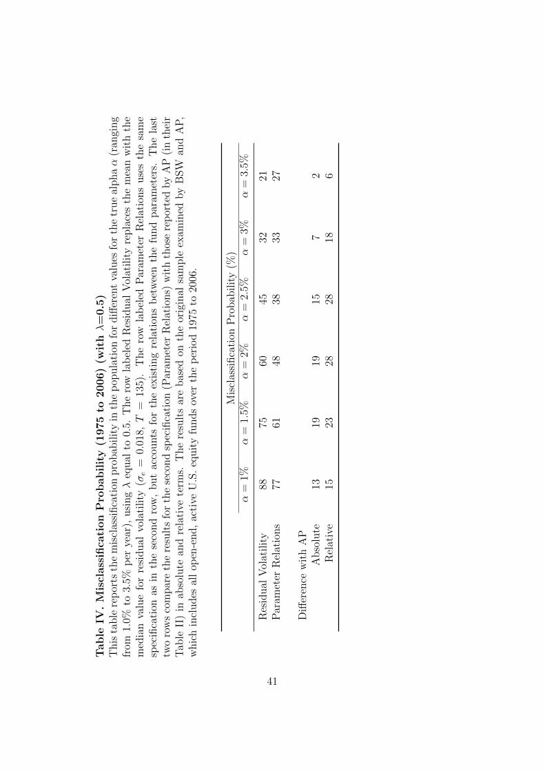
In Table IV, we examine the effect of these changes on the misclassification

probability. In the row labelled Residual Volatility, we use equation (13) to

compute δ(λ) (with σe = 0.018, T = 135, λ = 0.5). In the row labelled

Parameter Relations, we compute δ(λ) using equation (14). In the last two

rows, we compare our results with those obtained by AP (reported in their

Table II).

We find that these changes have a favorable impact on the performance

of the FDR proportions. For instance, the probability of misclassifying funds

14This finding resonates with the empirical evidence (Figure 1 and Table II) in Kosowski

et al. (2006).

21

with an alpha of 2% per year is equal to 48% using the second specification

(Parameter Relations), which represents a 28% reduction relative to AP ((67-

48)/67=0.28). Consistent with intuition, we also find that accounting for the

relations between parameters materially improves the detection of funds with

low alphas (i.e., those with αann between 1% and 2% per year).

Please insert Table IV here

A.2. The Choice of the Interval I(λ)

We now revisit the choice of interval I(λ) used by BSW and AP, and

examine its impact on the FDR proportions. Choosing λ ∈ (0, 1) involves

a trade-off between the mean and variance of the FDR proportions. To

elaborate, a higher λ lowers the bias of π̂0(λ) because I(λ) includes the t-

statistics of fewer nonzero alpha funds (i.e., δ(λ) grows small). However, it

also increases the variance of π̂0(λ) because I(λ) contains a smaller number

of fund t-statistics.

BSW account for this trade-off by using the method of Storey (2002) and

choosing λ based on the estimated MSE of π̂0(λ) (p. 189). In addition, BSW

impose an upper bound on λ at 0.7 to guarantee a conservative (biased)

estimator of π0. AP use exactly the same procedure to maintain consistency

with BSW.

Using this particular procedure makes sense in the context of BSW be-

cause they use the FDR as a multiple testing approach (as discussed in

Section I.A above). As a result, it is desirable to obtain a conservative esti-

mator π̂0(λ) to guarantee strong control of the Type I error in the selection

22

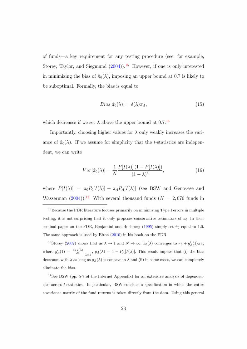
of funds—a key requirement for any testing procedure (see, for example,

Storey, Taylor, and Siegmund (2004)).15 However, if one is only interested

in minimizing the bias of π̂0(λ), imposing an upper bound at 0.7 is likely to

be suboptimal. Formally, the bias is equal to

Bias[π̂0(λ)] = δ(λ)πA, (15)

which decreases if we set λ above the upper bound at 0.7.16

Importantly, choosing higher values for λ only weakly increases the vari-

ance of π̂0(λ). If we assume for simplicity that the t-statistics are indepen-

dent, we can write

V ar[π̂0(λ)] =1

N

P [I(λ)] (1− P [I(λ)])

(1− λ)2, (16)

where P [I(λ)] = π0P0[I(λ)] + πAPA[I(λ)] (see BSW and Genovese and

Wasserman (2004)).17 With several thousand funds (N = 2, 076 funds in

15Because the FDR literature focuses primarily on minimizing Type I errors in multiple

testing, it is not surprising that it only proposes conservative estimators of π0. In their

seminal paper on the FDR, Benjamini and Hochberg (1995) simply set π̂0 equal to 1.0.

The same approach is used by Efron (2010) in his book on the FDR.

16Storey (2002) shows that as λ → 1 and N → ∞, π̂0(λ) converges to π0 + g′A(1)πA,

where g′A(1) = dgA(λ)dλ

∣∣∣λ=1

, gA(λ) = 1 − PA[I(λ)]. This result implies that (i) the bias

decreases with λ as long as gA(λ) is concave in λ and (ii) in some cases, we can completely

eliminate the bias.

17See BSW (pp. 5-7 of the Internet Appendix) for an extensive analysis of dependen-

cies across t-statistics. In particular, BSW consider a specification in which the entire

covariance matrix of the fund returns is taken directly from the data. Using this general

23

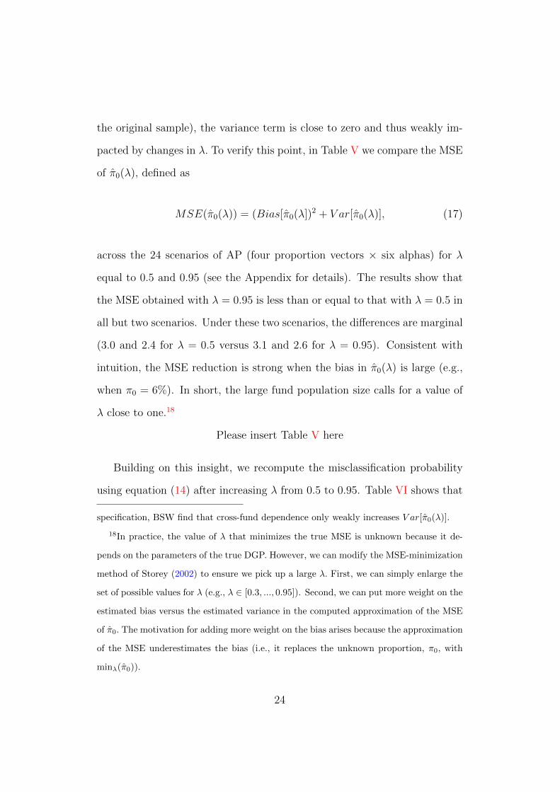
the original sample), the variance term is close to zero and thus weakly im-

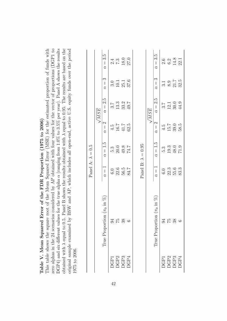
pacted by changes in λ. To verify this point, in Table V we compare the MSE

of π̂0(λ), defined as

MSE(π̂0(λ)) = (Bias[π̂0(λ])2 + V ar[π̂0(λ)], (17)

across the 24 scenarios of AP (four proportion vectors × six alphas) for λ

equal to 0.5 and 0.95 (see the Appendix for details). The results show that

the MSE obtained with λ = 0.95 is less than or equal to that with λ = 0.5 in

all but two scenarios. Under these two scenarios, the differences are marginal

(3.0 and 2.4 for λ = 0.5 versus 3.1 and 2.6 for λ = 0.95). Consistent with

intuition, the MSE reduction is strong when the bias in π̂0(λ) is large (e.g.,

when π0 = 6%). In short, the large fund population size calls for a value of

λ close to one.18

Please insert Table V here

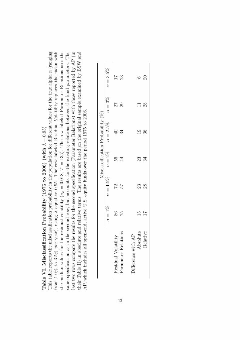
Building on this insight, we recompute the misclassification probability

using equation (14) after increasing λ from 0.5 to 0.95. Table VI shows that

specification, BSW find that cross-fund dependence only weakly increases V ar[π̂0(λ)].

18In practice, the value of λ that minimizes the true MSE is unknown because it de-

pends on the parameters of the true DGP. However, we can modify the MSE-minimization

method of Storey (2002) to ensure we pick up a large λ. First, we can simply enlarge the

set of possible values for λ (e.g., λ ∈ [0.3, ..., 0.95]). Second, we can put more weight on the

estimated bias versus the estimated variance in the computed approximation of the MSE

of π̂0. The motivation for adding more weight on the bias arises because the approximation

of the MSE underestimates the bias (i.e., it replaces the unknown proportion, π0, with

minλ(π̂0)).

24

a more careful choice of λ further improves the performance of the FDR

estimated proportions. For instance, the misclassification probability of a

fund with an alpha of 2% per year drops to 44% under the second specification

(Parameter Relations), which represents a 34% decrease relative to AP ((67-

44)/67=0.34).

Please insert Table VI here

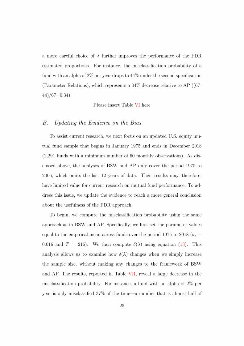
B. Updating the Evidence on the Bias

To assist current research, we next focus on an updated U.S. equity mu-

tual fund sample that begins in January 1975 and ends in December 2018

(2,291 funds with a minimum number of 60 monthly observations). As dis-

cussed above, the analyses of BSW and AP only cover the period 1975 to

2006, which omits the last 12 years of data. Their results may, therefore,

have limited value for current research on mutual fund performance. To ad-

dress this issue, we update the evidence to reach a more general conclusion

about the usefulness of the FDR approach.

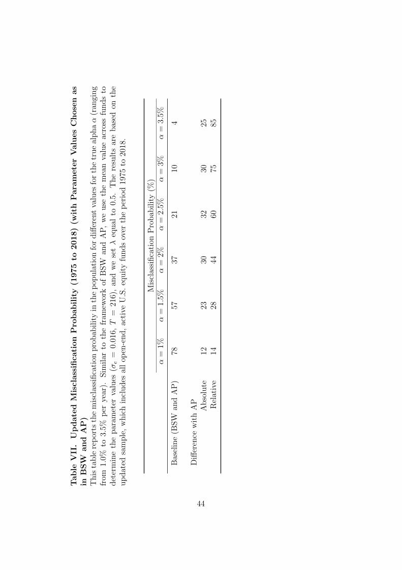
To begin, we compute the misclassification probability using the same

approach as in BSW and AP. Specifically, we first set the parameter values

equal to the empirical mean across funds over the period 1975 to 2018 (σe =

0.016 and T = 216). We then compute δ(λ) using equation (13). This

analysis allows us to examine how δ(λ) changes when we simply increase

the sample size, without making any changes to the framework of BSW

and AP. The results, reported in Table VII, reveal a large decrease in the

misclassification probability. For instance, a fund with an alpha of 2% per

year is only misclassified 37% of the time—a number that is almost half of

25

that documented by AP (67%).

Please insert Table VII here

Next, we reexamine the relation between the different parameters over

the updated sample. Similar to the results for the period 1975 to 2006,

Table VIII shows that the fund parameters are related—lower values of α

come with lower values of σe and higher values of T .

Please insert Table VIII here

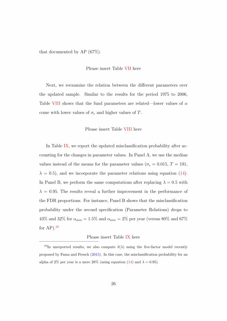
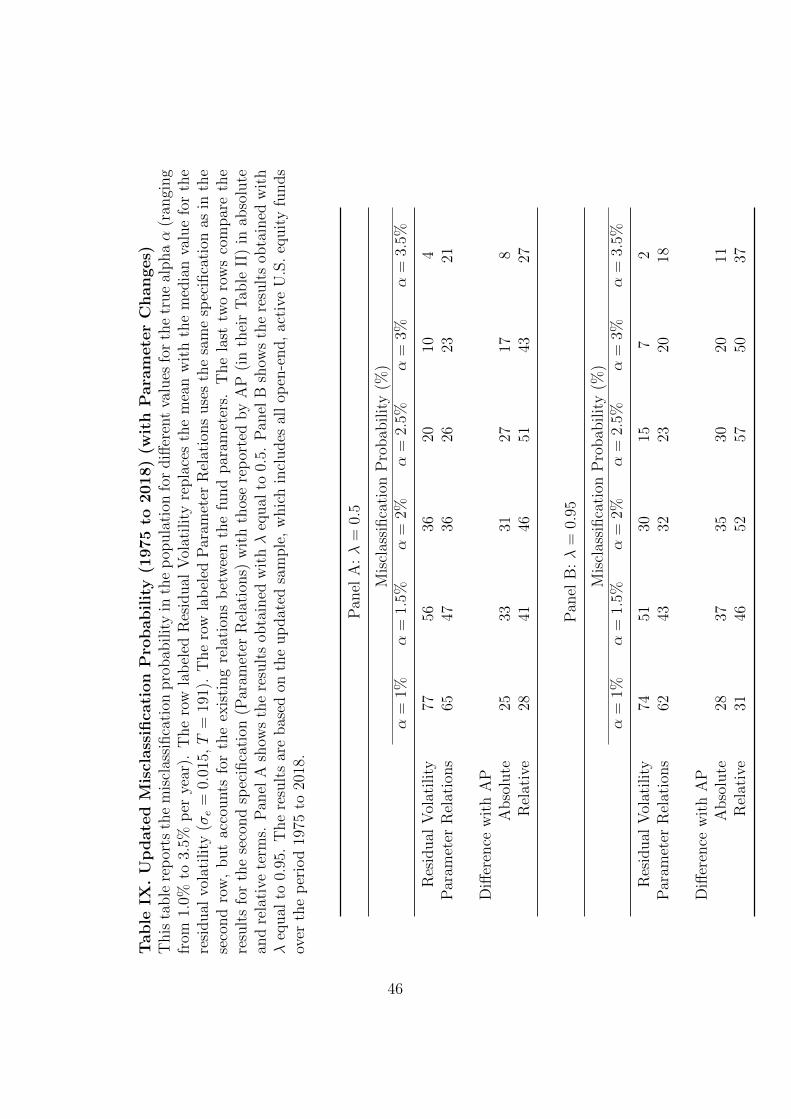
In Table IX, we report the updated misclassification probability after ac-

counting for the changes in parameter values. In Panel A, we use the median

values instead of the means for the parameter values (σe = 0.015, T = 191,

λ = 0.5), and we incorporate the parameter relations using equation (14).

In Panel B, we perform the same computations after replacing λ = 0.5 with

λ = 0.95. The results reveal a further improvement in the performance of

the FDR proportions. For instance, Panel B shows that the misclassification

probability under the second specification (Parameter Relations) drops to

43% and 32% for αann = 1.5% and αann = 2% per year (versus 80% and 67%

for AP).19

Please insert Table IX here

19In unreported results, we also compute δ(λ) using the five-factor model recently

proposed by Fama and French (2015). In this case, the misclassification probability for an

alpha of 2% per year is a mere 28% (using equation (14) and λ = 0.95).

26

Finally, we quantify the bias of the FDR proportions estimators across a

wide range of scenarios. Specifically, we consider 10 values for the proportion

vector (π0, π−A , π

+A)′ and six values for the true alpha of nonzero alpha funds,

which yields a total of 60 scenarios.20 We start by setting π0 equal to 95%

and decreasing it by increments of 10%, that is, π0 = {95%, 85%, ..., 5%}.

Then, for each value of π0, we follow AP and determine π−A and π+A such that

the ratio π−A/π+A is equal to 11.5.

Table X reports the average values of π̂0(λ), π̂−A(λ), and π̂+A(λ) for each

of the 60 scenarios using λ = 0.95. In about half of the scenarios (27 out

of 60), the bias of π̂0(λ) is lower than 10%, which implies that the FDR

approach provides a relevant representation of performance in the mutual

fund industry. The only scenarios in which the bias rises above 20% feature

a large proportion of nonzero alpha funds with low alphas or, equivalently,

funds that become increasingly similar to zero alpha funds (i.e., both π0 and

α are low). In other words, the bias can grow large in specific scenarios.

However, when it does, it also loses its economic significance—separating

zero and nonzero alpha funds becomes less relevant when these funds become

increasingly similar.

Please insert Table X here

20Our analysis gives equal weight to the different values of π0 and thus covers a larger

set of scenarios than AP (60 versus 24).

27

C. Summary of the Results

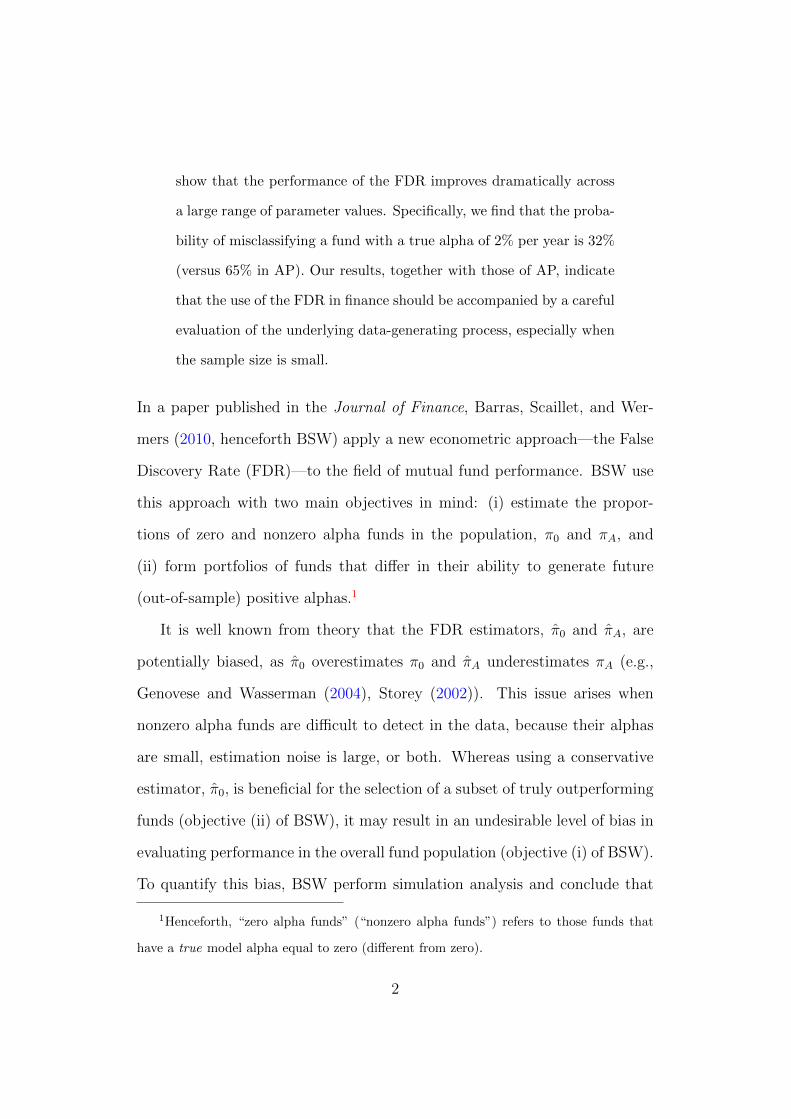
Our main findings are summarized in Figure 1. We plot the misclassifica-

tion probability as a function of the alpha for both the original sample (Panel

A) and the updated sample (Panel B). We introduce each of our changes in

a sequential manner to evaluate its marginal impact on δ(λ), that is, we

first use the median residual volatility, we next also account for the relations

between parameters, and finally we increase λ from 0.5 to 0.95.

Please insert Figure 1 here

Our analysis of the original sample (1975 to 2006) incorporates the main

points raised by AP but argues that additional changes are also necessary.

First, modifying the parameter values is important to capture the salient

features of mutual fund data. Second, increasing the value of λ improves

the performance of the FDR proportions. With these changes, the overall

evidence documented here provides a more nuanced view relative to BSW

and AP. In particular, whereas we confirm that the initial analysis of BSW

may be too optimistic, we do not find the high levels of bias documented by

AP.

Our analysis of the updated sample provides a clearer picture of the

performance of the FDR. The misclassification probability decreases signifi-

cantly, and the bias of the FDR proportions estimators is low across a wide

range of scenarios. We therefore conclude that the FDR approach is useful

for current research in the field of mutual fund performance. The results

represent good news for the academic community, which typically favors

28

statistical methods that are simple and fast—two major advantages of the

FDR approach. They also call for further research on the pros and cons of

the different methods for estimating the cross-sectional distributions of fund

alphas, which include the FDR as well as the parametric/Bayesian and non-

parametric approaches proposed in the literature (e.g., Barras, Gagliardini,

and Scaillet (2019), Harvey and Liu (2018), Jones and Shanken (2005)).

29

Appendix

A. The Bias of the Proportions on Nonzero Alpha Funds

As discussed in Section I.B, the estimated proportions of funds with neg-

ative/positive alphas are given by

π̂−A(λ) = P̂ [I−n (λ)]− π̂0(λ)P0[I−n (λ)], (A1)

π̂+A(λ) = P̂ [I+n (λ)]− π̂0(λ)P0[I

+n (λ)]. (A2)

Taking the expectations of P̂ [I−n (λ)] and P̂ [I+n (λ)], we obtain

P̂ [I−n (λ)] = P−A [I−n (λ)]π−A + P0[I−n (λ)]π0 + P+

A [I−n (λ)]π+A , (A3)

P̂ [I+n (λ)] = P+A [I+n (λ)]π+

A + P0[I+n (λ)]π0 + P−A [I+n (λ)]π−A , (A4)

where P−A [I−n (λ)] and P−A [I+n (λ)] denote the probabilities that the t-statistic

of a negative alpha fund falls in the interval I−n (λ) and I+n (λ). Similarly,

P+A [I−n (λ)] and P+

A [I+n (λ)] denote the probabilities that the t-statistic of a

positive alpha fund falls in the interval I−n (λ) and I+n (λ). Inserting these

expressions into equations (A1) and (A2) and replacing E[π̂0(λ)] with π0 +

δ(λ)πA, we obtain

E[π̂−A(λ)] = P−A [I−n (λ)]π−A − δ(λ)P0[I−n (λ)]πA + P+

A [I−n (λ)]π+A , (A5)

E[π̂+A(λ)] = P+

A [I+n (λ)]π+A − δ(λ)P0[I

+n (λ)]πA + P−A [I+n (λ)]π−A . (A6)

30

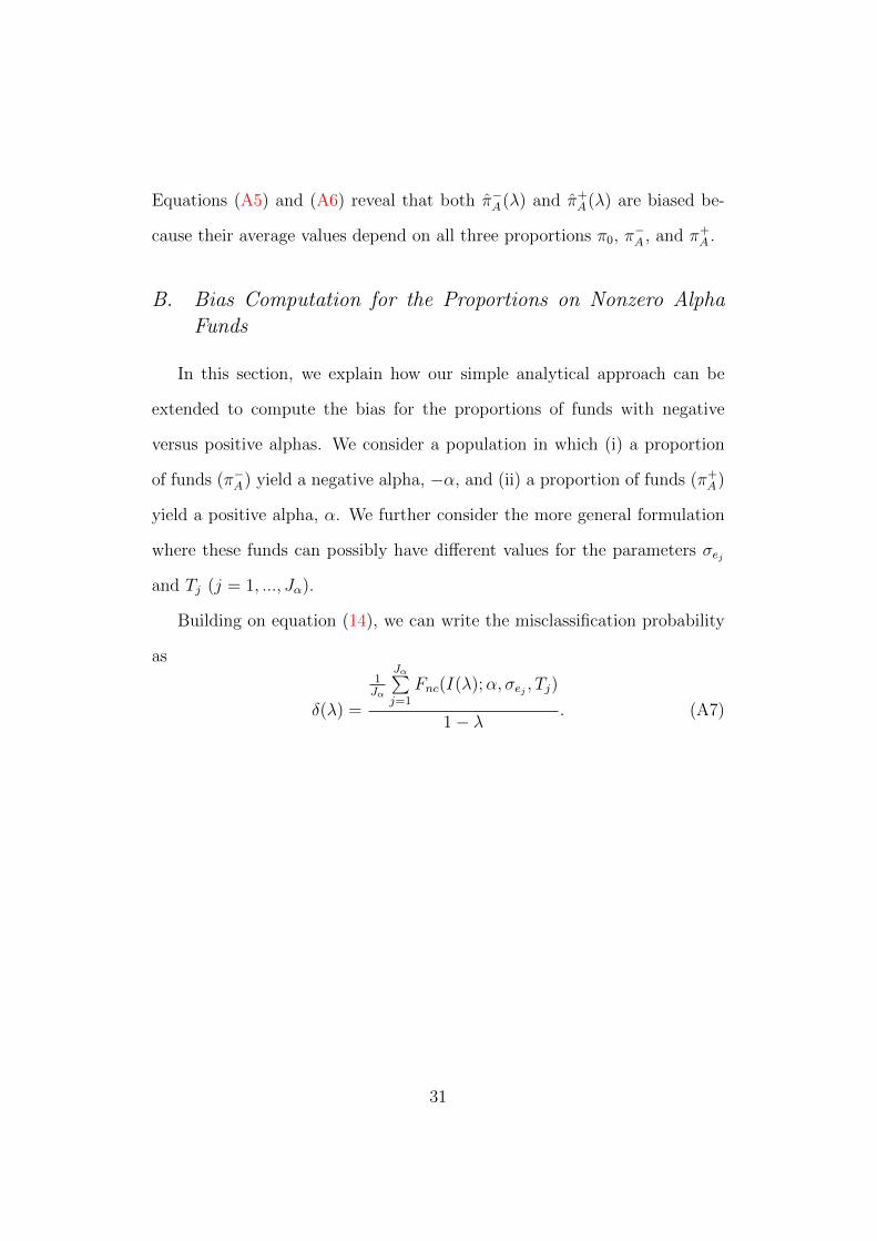
Equations (A5) and (A6) reveal that both π̂−A(λ) and π̂+A(λ) are biased be-

cause their average values depend on all three proportions π0, π−A , and π+

A .

B. Bias Computation for the Proportions on Nonzero AlphaFunds

In this section, we explain how our simple analytical approach can be

extended to compute the bias for the proportions of funds with negative

versus positive alphas. We consider a population in which (i) a proportion

of funds (π−A) yield a negative alpha, −α, and (ii) a proportion of funds (π+A)

yield a positive alpha, α. We further consider the more general formulation

where these funds can possibly have different values for the parameters σej

and Tj (j = 1, ..., Jα).

Building on equation (14), we can write the misclassification probability

as

δ(λ) =

1Jα

Jα∑j=1

Fnc(I(λ);α, σej , Tj)

1− λ. (A7)

31

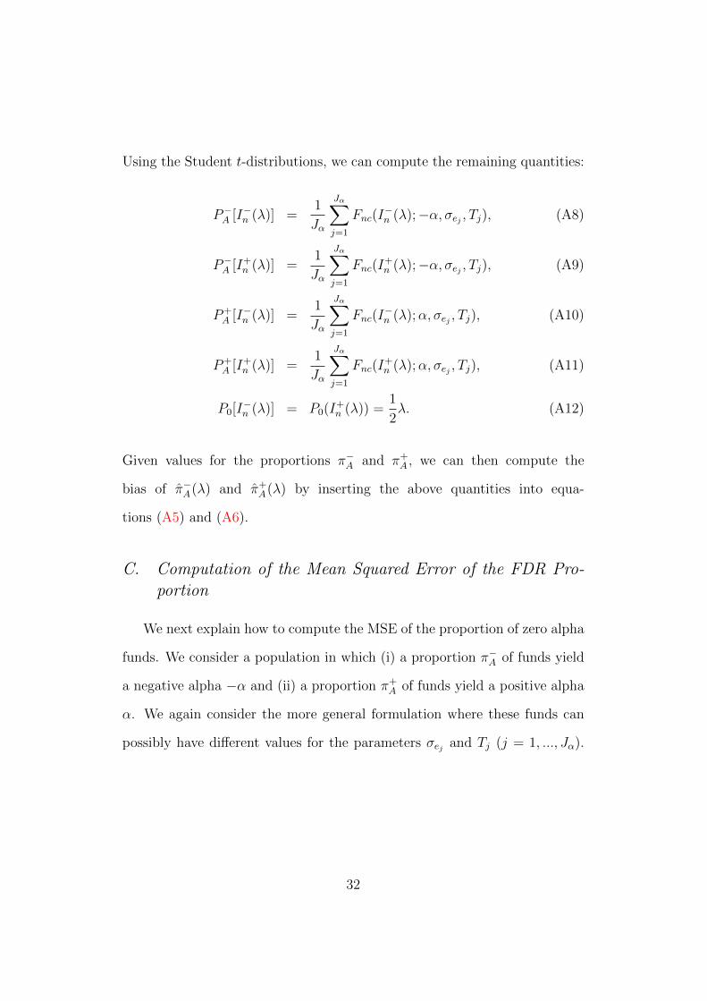
Using the Student t-distributions, we can compute the remaining quantities:

P−A [I−n (λ)] =1

Jα

Jα∑j=1

Fnc(I−n (λ);−α, σej , Tj), (A8)

P−A [I+n (λ)] =1

Jα

Jα∑j=1

Fnc(I+n (λ);−α, σej , Tj), (A9)

P+A [I−n (λ)] =

1

Jα

Jα∑j=1

Fnc(I−n (λ);α, σej , Tj), (A10)

P+A [I+n (λ)] =

1

Jα

Jα∑j=1

Fnc(I+n (λ);α, σej , Tj), (A11)

P0[I−n (λ)] = P0(I

+n (λ)) =

1

2λ. (A12)

Given values for the proportions π−A and π+A , we can then compute the

bias of π̂−A(λ) and π̂+A(λ) by inserting the above quantities into equa-

tions (A5) and (A6).

C. Computation of the Mean Squared Error of the FDR Pro-portion

We next explain how to compute the MSE of the proportion of zero alpha

funds. We consider a population in which (i) a proportion π−A of funds yield

a negative alpha −α and (ii) a proportion π+A of funds yield a positive alpha

α. We again consider the more general formulation where these funds can

possibly have different values for the parameters σej and Tj (j = 1, ..., Jα).

32

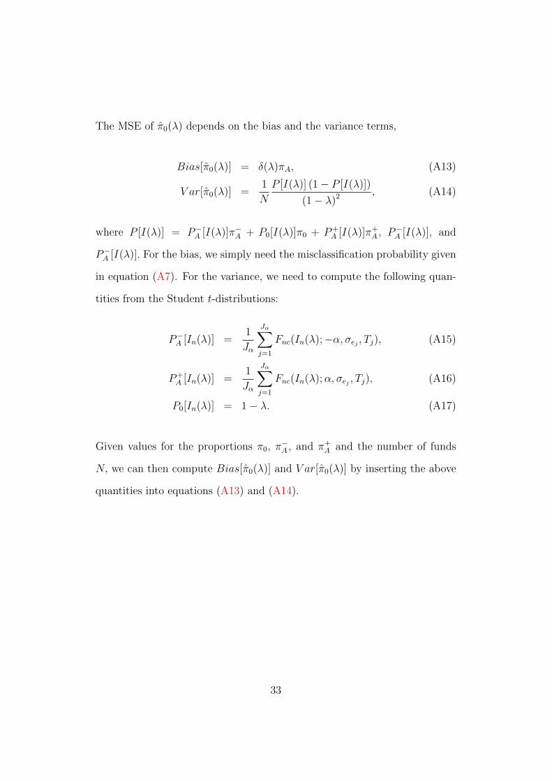
The MSE of π̂0(λ) depends on the bias and the variance terms,

Bias[π̂0(λ)] = δ(λ)πA, (A13)

V ar[π̂0(λ)] =1

N

P [I(λ)] (1− P [I(λ)])

(1− λ)2, (A14)

where P [I(λ)] = P−A [I(λ)]π−A + P0[I(λ)]π0 + P+A [I(λ)]π+

A , P−A [I(λ)], and

P−A [I(λ)]. For the bias, we simply need the misclassification probability given

in equation (A7). For the variance, we need to compute the following quan-

tities from the Student t-distributions:

P−A [In(λ)] =1

Jα

Jα∑j=1

Fnc(In(λ);−α, σej , Tj), (A15)

P+A [In(λ)] =

1

Jα

Jα∑j=1

Fnc(In(λ);α, σej , Tj), (A16)

P0[In(λ)] = 1− λ. (A17)

Given values for the proportions π0, π−A , and π+

A and the number of funds

N, we can then compute Bias[π̂0(λ)] and V ar[π̂0(λ)] by inserting the above

quantities into equations (A13) and (A14).

33

REFERENCES

Andrikogiannopoulou, Angie, and Filippos Papakonstantinou, 2019, Re-

assessing false discoveries in mutual fund performance: Skill, luck, or lack

of power? The Journal of Finance 74, Replications and Corrigenda, 2667–

2688.

Augustin, Patrick, Menachem Brenner, and Marti G. Subrahmanyam, 2019,

Informed options trading prior to takeover announcements: Insider trad-

ing? Management Science 65, 5697–5720.

Bajgrowicz, Pierre, and Olivier Scaillet, 2012, Technical trading revisited:

False discoveries, persistence tests, and transaction costs, Journal of Fi-

nancial Economics 106, 473–491.

Bajgrowicz, Pierre, Olivier Scaillet, and Adrien Treccani, 2016, Jumps in

high-frequency data: Spurious detections, dynamics, and news, Manage-

ment Science 62, 2198–2217.

Barras, Laurent, 2019, A large-scale approach for evaluating asset pricing

models, Journal of Financial Economics 134, 549–569.

Barras, Laurent, Patrick Gagliardini, and Olivier Scaillet, 2019, Skill and

value creation in the mutual fund industry, Swiss Finance Institute Re-

search Paper No. 18-66.

Barras, Laurent, Olivier Scaillet, and Russ Wermers, 2010, False discoveries

in mutual fund performance: Measuring luck in estimated alphas, The

Journal of Finance 65, 179–216.

34

Benjamini, Yoav, and Yosef Hochberg, 1995, Controlling the false discovery

rate: A practical and powerful approach to multiple testing, Journal of the

Royal Statistical Society: Series B (Methodological) 57, 289–300.

Berk, Jonathan B., and Richard C. Green, 2004, Mutual fund flows and

performance in rational markets, Journal of Political Economy 112, 1269–

1295.

Chen, Yong, Michael Cliff, and Haibei Zhao, 2017, Hedge funds: The good,

the bad, and the lucky, Journal of Financial and Quantitative Analysis 52,

1081–1109.

Cuthbertson, Keith, Dirk Nitzsche, and Niall O’Sullivan, 2008, UK mutual

fund performance: Skill or luck? Journal of Empirical Finance 15, 613–

634.

Efron, Bradley, 2010, Large-scale inference: Empirical Bayes methods for

estimation, testing, and prediction (Cambridge University Press, NY).

Fama, Eugene F., and Kenneth R. French, 2015, A five-factor asset pricing

model, Journal of Financial Economics 116, 1–22.

Ferson, Wayne, and Yong Chen, 2020, How many good and bad fund man-

agers are there, really? in C.F. Lee, ed., Handbook of Financial Economet-

rics, Mathematics, Statistics, and Machine Learning , volume 4, chapter

108, 3757–3831 (World Scientific Publishing, NJ).

Genovese, Christopher, and Larry Wasserman, 2004, A stochastic process

35

approach to false discovery control, The Annals of Statistics 32, 1035–

1061.

Giglio, Stefano, Yuan Liao, and Dacheng Xiu, 2019, Thousands of alpha

tests, Chicago Booth Research Paper 2018–16.

Harvey, Campbell R., and Yan Liu, 2018, Detecting repeatable performance,

The Review of Financial Studies 31, 2499–2552.

Harvey, Campbell R., Yan Liu, and Heqing Zhu, 2016, ...and the cross-section

of expected returns, The Review of Financial Studies 29, 5–68.

Jones, Christopher S., and Jay Shanken, 2005, Mutual fund performance

with learning across funds, Journal of Financial Economics 78, 507–552.

Kosowski, Robert, Allan Timmermann, Russ Wermers, and Hal White, 2006,

Can mutual fund “stars” really pick stocks? New evidence from a boot-

strap analysis, The Journal of Finance 61, 2551–2595.

Scaillet, Olivier, Adrien Treccani, and Christopher Trevisan, forthcoming,

High-frequency jump analysis of the bitcoin market, Journal of Financial

Econometrics .

Stambaugh, Robert F., 2014, Presidential address: Investment noise and

trends, The Journal of Finance 69, 1415–1453.

Storey, John D., 2002, A direct approach to false discovery rates, Journal of

the Royal Statistical Society: Series B (Statistical Methodology) 64, 479–

498.

36

Storey, John D., Jonathan E. Taylor, and David Siegmund, 2004, Strong

control, conservative point estimation and simultaneous conservative con-

sistency of false discovery rates: A unified approach, Journal of the Royal

Statistical Society: Series B (Statistical Methodology) 66, 187–205.

Treynor, Jack L., and Fischer Black, 1973, How to use security analysis to

improve portfolio selection, The Journal of Business 46, 66–86.

37

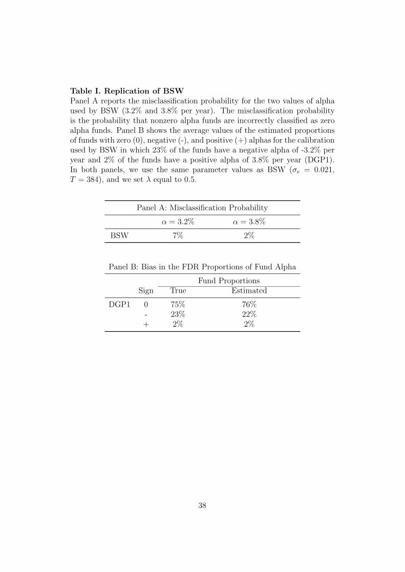
Table I. Replication of BSWPanel A reports the misclassification probability for the two values of alphaused by BSW (3.2% and 3.8% per year). The misclassification probabilityis the probability that nonzero alpha funds are incorrectly classified as zeroalpha funds. Panel B shows the average values of the estimated proportionsof funds with zero (0), negative (-), and positive (+) alphas for the calibrationused by BSW in which 23% of the funds have a negative alpha of -3.2% peryear and 2% of the funds have a positive alpha of 3.8% per year (DGP1).In both panels, we use the same parameter values as BSW (σe = 0.021,T = 384), and we set λ equal to 0.5.

Panel A: Misclassification Probability

α = 3.2% α = 3.8%

BSW 7% 2%

Panel B: Bias in the FDR Proportions of Fund Alpha

Fund ProportionsSign True Estimated

DGP1 0 75% 76%- 23% 22%+ 2% 2%

38

Tab

leII

.R

epli

cati

on

of

AP

Pan

elA

rep

orts

the

mis

clas

sifica

tion

pro

bab

ilit

yfo

rdiff

eren

tva

lues

use

dby

AP

for

the

true

alpha

(fro

m1.

0%to

3.5%

per

year

).P

anel

Bsh

ows

the

aver

age

valu

esof

the

esti

mat

edpro

por

tion

sof

funds

wit

hze

ro(0

),neg

ativ

e(-

),an

dp

osit

ive

(+)

alphas

inth

e24

scen

ario

sco

nsi

der

edby

AP

obta

ined

wit

hfo

ur

valu

esfo

rth

eve

ctor

ofpro

por

tion

s(D

GP

1to

DG

P4)

and

six

valu

esfo

rth

etr

ue

alphaα

(ran

ging

from

1.0%

to3.

5%p

erye

ar).

Inb

oth

pan

els,

we

use

the

sam

epar

amet

erva

lue

asA

P(σ

e=

0.02

1,T

=15

0),

and

we

setλ

equal

to0.

5.

Pan

elA

:M

iscl

assi

fica

tion

Pro

bab

ilit

y

α=

1%α

=1.

5%α

=2%

α=

2.5%

α=

3%α

=3.

5%

AP

90%

80%

67%

53%

40%

29%

Pan

elB

:B

ias

inth

eF

DR

Pro

por

tion

s

Fund

Alp

ha

Est

imat

edP

rop

orti

ons

(%)

Sig

nT

rue

Pro

por

tion

s(%

)α

=1%

α=

1.5%

α=

2%α

=2.

5%α

=3%

α=

3.5%

DG

P1

094

9999

9897

9696

-6

11

23

44

+1

00

00

00

DG

P2

075

9895

9288

8582

-23

25

812

1518

+2

00

00

00

DG

P3

038

9487

7971

6355

-58

613

2129

3744

+5

00

00

00

DG

P4

06

9181

6956

4433

-86

919

3144

5666

+8

00

00

00

39

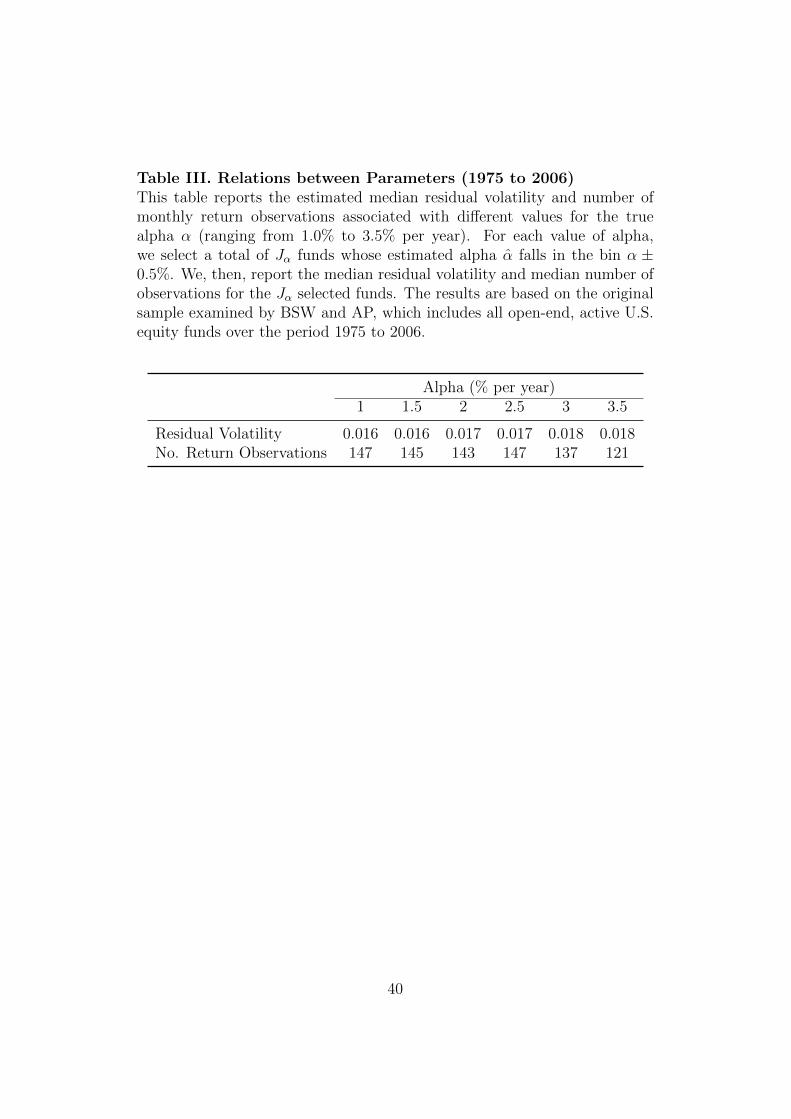
Table III. Relations between Parameters (1975 to 2006)This table reports the estimated median residual volatility and number ofmonthly return observations associated with different values for the truealpha α (ranging from 1.0% to 3.5% per year). For each value of alpha,we select a total of Jα funds whose estimated alpha α̂ falls in the bin α ±0.5%. We, then, report the median residual volatility and median number ofobservations for the Jα selected funds. The results are based on the originalsample examined by BSW and AP, which includes all open-end, active U.S.equity funds over the period 1975 to 2006.

Alpha (% per year)1 1.5 2 2.5 3 3.5

Residual Volatility 0.016 0.016 0.017 0.017 0.018 0.018No. Return Observations 147 145 143 147 137 121

40

Tab

leIV

.M

iscl

ass

ifica

tion

Pro

babil

ity

(1975

to2006)

(wit

hλ=

0.5

)T

his

table

rep

orts

the

mis

clas

sifica

tion

pro

bab

ilit

yin

the

pop

ula

tion

for

diff

eren

tva

lues

for

the

true

alphaα

(ran

ging

from

1.0%

to3.

5%p

erye

ar),

usi

ngλ

equal

to0.

5.T

he

row

lab

eled

Res

idual

Vol

atilit

yre

pla

ces

the

mea

nw

ith

the

med

ian

valu

efo

rre

sidual

vola

tility

(σe

=0.

018,T

=13

5).

The

row

lab

eled

Par

amet

erR

elat

ions

use

sth

esa

me

spec

ifica

tion

asin

the

seco

nd

row

,but

acco

unts

for

the

exis

ting

rela

tion

sb

etw

een

the

fund

par

amet

ers.

The

last

two

row

sco

mpar

eth

ere

sult

sfo

rth

ese

cond

spec

ifica

tion

(Par

amet

erR

elat

ions)

wit

hth

ose

rep

orte

dby

AP

(in

thei

rT

able

II)

inab

solu

tean

dre

lati

vete

rms.

The

resu

lts

are

bas

edon

the

orig

inal

sam

ple

exam

ined

by

BSW

and

AP

,w

hic

hin

cludes

all

open

-end,

acti

veU

.S.

equit

yfu

nds

over

the

per

iod

1975

to20

06.

Mis

clas

sifica

tion

Pro

bab

ilit

y(%

)α

=1%

α=

1.5%

α=

2%α

=2.

5%α

=3%

α=

3.5%

Res

idual

Vol

atilit

y88

7560

4532

21P

aram

eter

Rel

atio

ns

7761

4838

3327

Diff

eren

cew

ith

AP

Abso

lute

1319

1915

72

Rel

ativ

e15

2328

2818

6

41

Tab

leV

.M

ean

Square

dE

rror

of

the

FD

RP

rop

ort

ion

(1975

to2006)

This

table

show

sth

esq

uar

ero

otof

the

Mea

nSquar

edE

rror

(MSE

)fo

rth

ees

tim

ated

pro

por

tion

offu

nds

wit

hze

roal

phas

inth

e24

scen

ario

sco

nsi

der

edby

AP

obta

ined

wit

hfo

ur

valu

esfo

rth

eve

ctor

ofpro

por

tion

s(D

GP

1to

DG

P4)

and

six

diff

eren

tva

lues

for

the

true

alphaα

(ran

ging

from

1.0%

to3.

5%p

erye

ar).

Pan

elA

show

sth

ere

sult

sob

tain

edw

ithλ

equal

to0.

5.P

anel

Bsh

ows

the

resu

lts

obta

ined

wit

hλ

equal

to0.

95.

The

resu

lts

are

bas

edon

the

orig

inal

sam

ple

exam

ined

by

BSW

and

AP

,w

hic

hin

cludes

all

open

-end,

acti

veU

.S.

equit

yfu

nds

over

the

per

iod

1975

to20

06.

Pan

elA

:λ

=0.

5√MSE

Tru

eP

rop

orti

on(π

0in

%)

α=

1α

=1.

5α

=2

α=

2.5

α=

3α

=3.

5

DG

P1

946.

05.

34.

53.

73.

02.

4D

GP

275

22.6

20.0

16.7

13.3

10.1

7.3

DG

P3

3856

.549

.841

.733

.225

.118

.0D

GP

46

84.7

74.7

62.5

49.7

37.6

27.0

Pan

elB

:λ

=0.

95√MSE

Tru

eP

rop

orti

on(π

0in

%)

α=

1α

=1.

5α

=2

α=

2.5

α=

3α

=3.

5

DG

P1

946.

05.

34.

53.

73.

12.

6D

GP

275

22.3

19.3

15.7

12.1

8.9

6.2

DG

P3

3855

.648

.039

.030

.021

.714

.8D

GP

46

83.3

71.9

58.5

44.9

32.5

22.1

42

Tab

leV

I.M

iscl

ass

ifica

tion

Pro

babil

ity

(1975

to2006)

(wit

hλ

=0.

95)

This

table

rep

orts

the

mis

clas

sifica

tion

pro

bab

ilit

yin

the

pop

ula

tion

for

diff

eren

tva

lues

for

the

true

alphaα

(ran

ging

from

1.0%

to3.

5%p

erye

ar),

usi

ngλ

equal

to0.

95.

The

row

lab

eled

Res

idual

Vol

atilit

yre

pla

ces

the

mea

nw

ith

the

med

ian

valu

esfo

rth

ere

sidual

vola

tility

(σe

=0.

018,T

=13

5).

The

row

lab

eled

Par

amet

erR

elat

ions

use

sth

esa

me

spec

ifica

tion

asin

the

seco

nd

row

,but

acco

unts

for

the

exis

ting

rela

tion

sb

etw

een

the

fund

par

amet

ers.

The

last

two

row

sco

mpar

eth

ere

sult

sfo

rth

ese

cond

spec

ifica

tion

(Par

amet

erR

elat

ions)

wit

hth

ose

rep

orte

dby

AP

(in

thei

rT

able

II)

inab

solu

tean

dre

lati

vete

rms.

The

resu

lts

are

bas

edon

the

orig

inal

sam

ple

exam

ined

by

BSW

and

AP

,w

hic

hin

cludes

all

open

-end,

acti

veU

.S.

equit

yfu

nds

over

the

per

iod

1975

to20

06.

Mis

clas

sifica

tion

Pro

bab

ilit

y(%

)α

=1%

α=

1.5%

α=

2%α

=2.

5%α

=3%

α=

3.5%

Res

idual

Vol

atilit

y86

7256

4027

17P

aram

eter

Rel

atio

ns

7557

4434

2923

Diff

eren

cew

ith

AP

Abso

lute

1523

2319

116

Rel

ativ

e17

2834

3628

20

43

Tab

leV

II.

Up

date

dM

iscl

ass

ifica

tion

Pro

babil

ity

(1975

to2018)

(wit

hP

ara

mete

rV

alu

es

Ch

ose

nas

inB

SW

and

AP

)T

his

table

rep

orts

the

mis

clas

sifica

tion

pro

bab

ilit

yin

the

pop

ula

tion

for

diff

eren

tva

lues

for

the

true

alphaα

(ran

ging

from

1.0%

to3.

5%p

erye

ar).

Sim

ilar

toth

efr

amew

ork

ofB

SW

and

AP

,w

euse

the

mea

nva

lue

acro

ssfu

nds

todet

erm

ine

the

par

amet

erva

lues

(σe

=0.

016,T

=21

6),

and

we

setλ

equal

to0.

5.T

he

resu

lts

are

bas

edon

the

up

dat

edsa

mple

,w

hic

hin

cludes

all

open

-end,

acti

veU

.S.

equit

yfu

nds

over

the

per

iod

1975

to20

18.

Mis

clas

sifica

tion

Pro

bab

ilit

y(%

)α

=1%

α=

1.5%

α=

2%α

=2.

5%α

=3%

α=

3.5%

Bas

elin

e(B

SW

and

AP

)78

5737

2110

4

Diff

eren

cew

ith

AP

Abso

lute

1223

3032

3025

Rel

ativ

e14

2844

6075

85

44

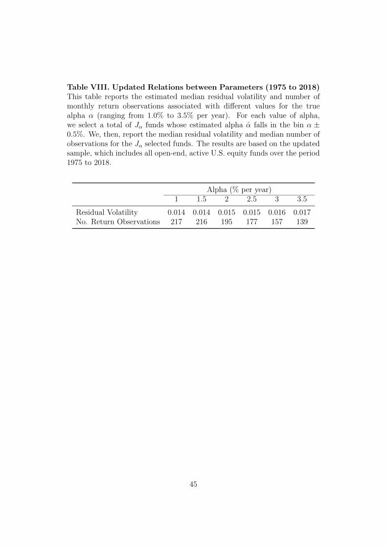
Table VIII. Updated Relations between Parameters (1975 to 2018)This table reports the estimated median residual volatility and number ofmonthly return observations associated with different values for the truealpha α (ranging from 1.0% to 3.5% per year). For each value of alpha,we select a total of Jα funds whose estimated alpha α̂ falls in the bin α ±0.5%. We, then, report the median residual volatility and median number ofobservations for the Jα selected funds. The results are based on the updatedsample, which includes all open-end, active U.S. equity funds over the period1975 to 2018.

Alpha (% per year)1 1.5 2 2.5 3 3.5

Residual Volatility 0.014 0.014 0.015 0.015 0.016 0.017No. Return Observations 217 216 195 177 157 139

45

Tab

leIX

.U

pdate

dM

iscl

ass

ifica

tion

Pro

babil

ity

(1975

to2018)

(wit

hP

ara

mete

rC

han

ges)

This

table

rep

orts

the

mis

clas

sifica

tion

pro

bab

ilit

yin

the

pop

ula

tion

for

diff

eren

tva

lues

for

the

true

alphaα

(ran

ging

from

1.0%

to3.

5%p

erye

ar).

The

row

lab

eled

Res

idual

Vol

atilit

yre

pla

ces

the

mea

nw

ith

the

med

ian

valu

efo

rth

ere

sidual

vola

tility

(σe

=0.

015,T

=19

1).

The

row

lab

eled

Par

amet

erR

elat

ions

use

sth

esa

me

spec

ifica

tion

asin

the

seco

nd

row

,but

acco

unts

for

the

exis

ting

rela

tion

sb

etw

een

the

fund

par

amet

ers.

The

last

two

row

sco

mpar

eth

ere

sult

sfo

rth

ese

cond

spec

ifica

tion

(Par

amet

erR

elat

ions)

wit

hth

ose

rep

orte

dby

AP

(in

thei

rT

able

II)

inab

solu

tean

dre

lati

vete

rms.

Pan

elA

show

sth

ere

sult

sob

tain

edw

ithλ

equal

to0.

5.P

anel

Bsh

ows

the

resu

lts

obta

ined

wit

hλ

equal

to0.

95.

The

resu

lts

are

bas

edon

the

up

dat

edsa

mple

,w

hic

hin

cludes

all

open

-end,

acti

veU

.S.

equit

yfu

nds

over

the

per

iod

1975

to20

18.

Pan

elA

:λ

=0.

5

Mis

clas

sifica

tion

Pro

bab

ilit

y(%

)α

=1%

α=

1.5%

α=

2%α

=2.

5%α

=3%

α=

3.5%

Res

idual

Vol

atilit

y77

5636

2010

4P

aram

eter

Rel

atio

ns

6547

3626

2321

Diff

eren

cew

ith

AP

Abso

lute

2533

3127

178

Rel

ativ

e28

4146

5143

27

Pan

elB

:λ

=0.

95

Mis

clas

sifica

tion

Pro

bab

ilit

y(%

)α

=1%

α=

1.5%

α=

2%α

=2.

5%α

=3%

α=

3.5%

Res

idual

Vol

atilit

y74

5130

157

2P

aram

eter

Rel

atio

ns

6243

3223

2018

Diff

eren

cew

ith

AP

Abso

lute

2837

3530

2011

Rel

ativ

e31

4652

5750

37

46

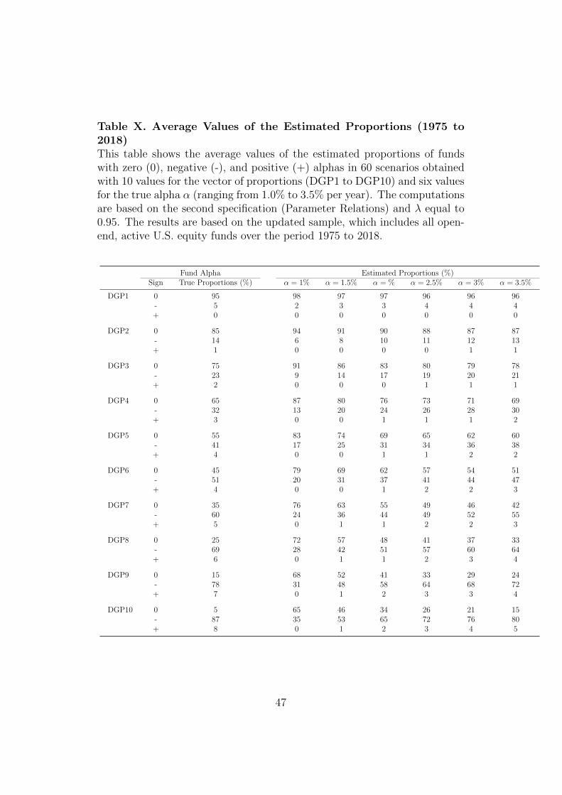
Table X. Average Values of the Estimated Proportions (1975 to2018)This table shows the average values of the estimated proportions of fundswith zero (0), negative (-), and positive (+) alphas in 60 scenarios obtainedwith 10 values for the vector of proportions (DGP1 to DGP10) and six valuesfor the true alpha α (ranging from 1.0% to 3.5% per year). The computationsare based on the second specification (Parameter Relations) and λ equal to0.95. The results are based on the updated sample, which includes all open-end, active U.S. equity funds over the period 1975 to 2018.

Fund Alpha Estimated Proportions (%)Sign True Proportions (%) α = 1% α = 1.5% α = % α = 2.5% α = 3% α = 3.5%

DGP1 0 95 98 97 97 96 96 96- 5 2 3 3 4 4 4+ 0 0 0 0 0 0 0

DGP2 0 85 94 91 90 88 87 87- 14 6 8 10 11 12 13+ 1 0 0 0 0 1 1

DGP3 0 75 91 86 83 80 79 78- 23 9 14 17 19 20 21+ 2 0 0 0 1 1 1

DGP4 0 65 87 80 76 73 71 69- 32 13 20 24 26 28 30+ 3 0 0 1 1 1 2

DGP5 0 55 83 74 69 65 62 60- 41 17 25 31 34 36 38+ 4 0 0 1 1 2 2

DGP6 0 45 79 69 62 57 54 51- 51 20 31 37 41 44 47+ 4 0 0 1 2 2 3

DGP7 0 35 76 63 55 49 46 42- 60 24 36 44 49 52 55+ 5 0 1 1 2 2 3

DGP8 0 25 72 57 48 41 37 33- 69 28 42 51 57 60 64+ 6 0 1 1 2 3 4

DGP9 0 15 68 52 41 33 29 24- 78 31 48 58 64 68 72+ 7 0 1 2 3 3 4

DGP10 0 5 65 46 34 26 21 15- 87 35 53 65 72 76 80+ 8 0 1 2 3 4 5

47

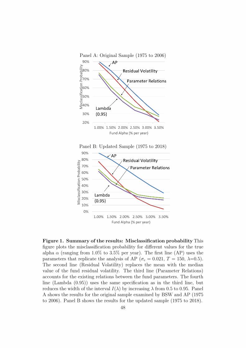
Panel A: Original Sample (1975 to 2006)

Panel B: Updated Sample (1975 to 2018)

Figure 1. Summary of the results: Misclassification probability Thisfigure plots the misclassification probability for different values for the truealpha α (ranging from 1.0% to 3.5% per year). The first line (AP) uses theparameters that replicate the analysis of AP (σe = 0.021, T = 150, λ=0.5).The second line (Residual Volatility) replaces the mean with the medianvalue of the fund residual volatility. The third line (Parameter Relations)accounts for the existing relations between the fund parameters. The fourthline (Lambda (0.95)) uses the same specification as in the third line, butreduces the width of the interval I(λ) by increasing λ from 0.5 to 0.95. PanelA shows the results for the original sample examined by BSW and AP (1975to 2006). Panel B shows the results for the updated sample (1975 to 2018).

48