Embed Size (px)
Citation preview

Artificial Intelligence 133 (2001) 139–188
Reasoning about nonlinear system identification
Elizabeth Bradleya,∗,1, Matthew Easleyb,1, Reinhard Stollec,2a Department of Computer Science, University of Colorado, Campus Box 430, Boulder, CO 80309-0430, USA
b Rockwell Science Center, 444 High Street, Suite 400, Palo Alto, CA 94301, USAc Xerox PARC, 3333 Coyote Hill Road, Palo Alto, CA 94304, USA
Received 19 May 2000; received in revised form 4 May 2001
Abstract
System identification is the process of deducing a mathematical model of the internal dynamics ofa system from observations of its outputs. The computer program PRET automates this process bybuilding a layer of artificial intelligence (AI) techniques around a set of traditional formal engineeringmethods. PRET takes a generate-and-test approach, using a small, powerfulmeta-domain theory thattailors the space of candidate models to the problem at hand. It then tests these models againstthe known behavior of the target system using a large set of more-general mathematical rules. Thecomplex interplay of heterogeneous reasoning modes that is involved in this process is orchestratedby a special first-order logic system that uses static abstraction levels, dynamic declarative metacontrol, and a simple form of truth maintenance in order to test models quickly and cheaply. Unlikeother modeling tools—most of which use libraries to model small, well-posed problems in limiteddomains and rely on their users to supply detailed descriptions of the target system—PRET workswith nonlinear systems in multiple domains and interacts directly with the real world via sensors andactuators. This approach has met with success in a variety of simulated and real applications, rangingfrom textbook systems to real-world engineering problems. 2001 Elsevier Science B.V. All rightsreserved.
Keywords: Automated model building; System identification; Qualitative reasoning; Qualitative physics;Knowledge representation framework; Reasoning framework; Input-output modeling
* Corresponding author.E-mail addresses: [email protected] (E. Bradley), [email protected] (M. Easley),
[email protected] (R. Stolle).1 Supported by NSF NYI #CCR-9357740, ONR #N00014-96-1-0720, and a Packard Fellowship in Science
and Engineering from the David and Lucile Packard Foundation.2 Research performed while a research assistant at the University of Colorado at Boulder and during a
postdoctoral fellowship at Stanford University funded by the German Academic Exchange Service (DAAD)“Gemeinsames Hochschulsonderprogramm III von Bund und Ländern”.
0004-3702/01/$ – see front matter 2001 Elsevier Science B.V. All rights reserved.PII: S0004-3702(01)00143-6

140 E. Bradley et al. / Artificial Intelligence 133 (2001) 139–188
1. Introduction
One of the most powerful analysis and design tools in existence—and often one ofthe most difficult to create—is a good model. Modeling is an essential first step in avariety of engineering problems. Faced with the task of designing a controller for arobot arm, for instance, a mechanical engineer performs a few simple experiments on thesystem, observes the resulting behavior, makes some informed guesses about what modelfragments could account for that behavior, and then combines those terms into a modeland checks it against the physical system. This model then becomes the mathematical coreof the controller. Accuracy is not the only requirement; for efficiency reasons, engineerswork hard to construct minimal models—those that ignore unimportant details and captureonly the behavior that is important for the task at hand. The subtlety of the reasoning skillsinvolved in this process, together with the intricacy of the interplay between them, has ledmany of its practitioners to classify modeling as “intuitive” and “an art” [69].
The computer program PRET, the topic of this paper, formalizes these intuitions andautomates a coherent and useful part of this art. PRET is an automated tool for nonlinearsystem identification. Its inputs are a set of observations of the outputs of a target system,some optional hypotheses about the physics involved, and a set of tolerances within whicha successful model must match the observations; its output is an ordinary differentialequation (ODE) model of the internal dynamics of that system. See Fig. 1 for a blockdiagram. PRET uses a small, powerful domain theory to build models and a larger, more-general mathematical theory to test them. It is designed to work in any domain that admitsODE models; adding a new domain is simply a matter of coding one or two simple domainrules. Its architecture wraps a layer of artificial intelligence (AI) techniques around a set oftraditional formal engineering methods. This AI layer incorporates a variety of reasoningmodes: qualitative reasoning, qualitative simulation, numerical simulation, geometricreasoning, constraint propagation, resolution, reasoning with abstraction levels, declarativemeta control, and a simple form of truth maintenance. Models are represented usinga component-based modeling framework that accommodates different domains, adaptssmoothly to varying amounts of domain knowledge, and allows expert users to createmodel-building frameworks for new application domains easily. An input-output modelingsubsystem allows PRET to observe target systems actively, manipulating actuators andreading sensors to perform experiments whose results augment its knowledge in a mannerthat is useful to the modeling problem that it is trying to solve. The entire reasoning process
Fig. 1. PRET combines AI and formal engineering techniques to build ODE models of nonlinear dynamicalsystems. It uses domain-specific knowledge to build models and an encoded ODE theory to test them, and itinteracts directly and autonomously with target systems using sensors and actuators.

E. Bradley et al. / Artificial Intelligence 133 (2001) 139–188 141
Fig. 2. The system identification (SID) process. Structural identification yields the general form of the model; inparameter estimation, values for the unknown coefficients in that model are determined. PRET automates bothphases of this process.
is orchestrated by a special first-order logic inference system, which automatically chooses,invokes, and interprets the results of the techniques that are appropriate for each point inthe model-building procedure. This combination of techniques lets PRET shift fluidly backand forth between domain-specific reasoning, general mathematics, and actual physicalexperiments in order to navigate efficiently through an exponential search space of possiblemodels.
In general, system identification proceeds in two interleaved phases: first,structuralidentification, in which the form of the differential equation is determined, and thenparameter estimation, in which values for the coefficients are obtained. If structuralidentification produces an incorrect ODE model, no coefficient values can make itssolutions match the sensor data. In this event, the structural identification process mustbe repeated—often using information about why the previous attempt failed—until theprocess converges to a solution, as shown diagrammatically in Fig. 2. In linear physicalsystems, structural identification and parameter estimation are fairly well understood.The difficulties—and the subtleties employed by practitioners—arise where noisy orincomplete data are involved, or where efficiency is an issue. See [59,66] for someexamples. Innonlinear systems, however, both procedures are vastly more difficult—thetype of material that is covered only in the last few pages of standard textbooks.
Unlike system identification software used in the control theory community, PRET is notjust an automated parameter estimator; rather, it uses sophisticated reasoning techniques toautomate the structural phase of model building as well. The basic paradigm is “generateand test”. PRET first uses its encoded domain theory—the upper ellipse in Fig. 1—toassemble combinations of user-specified and automatically generated ODE fragments intoa candidate model. In a mechanics problem, for instance, the generate phase uses Newton’slaws to combine force terms; in electronics, it uses Kirchhoff’s laws to sum voltages in aloop or currents in a cutset. In order to test a candidate model, PRET performs a series ofinferences about the model and the observations that the model is to match. This processis guided by two important assumptions: that abstract reasoning should be chosen over

142 E. Bradley et al. / Artificial Intelligence 133 (2001) 139–188
lower-level techniques, and that any model that cannot be proved wrong is right. PRET’sinference engine uses an encoded mathematical theory (the lower ellipse in Fig. 1) to searchfor contradictions in the sets of facts inferred from the model and from the observations. AnODE that is linear, for instance, cannot account for chaotic behavior; such a model shouldfail the test if the target system has been observed to be chaotic. Furthermore, establishingwhether an ODE is linear is a matter of simple symbolic algebra, so the inference engineshould not resort to a numerical integration to establish this contradiction. Like the domaintheory, PRET’s ODE theory is designed to be easily extended by an expert user.
To make these ideas more concrete, consider the spring/mass system shown at the topright of Fig. 3. To instruct PRET to build a model of this system, a user would enterthe find-model call at the left of the figure. (PRET also has a GUI that leads usersthrough this interaction without subjecting them to this syntax.) Thedomain statementinstantiates the relevant domain theory; the next two lines inform PRET that the system
Fig. 3. Modeling a simple spring/mass system. In this example call to PRET, the user first sets up the problem, thenmakes five observations about the position coordinatesq1 andq2, hypothesizes nine different force terms, andfinally specifies resolution and range criteria that a successful model must satisfy. Angle brackets (e.g.,<time>)identify state variables and other special keywords that play roles in PRET’s use of its domain theory. We useteletype font in the body of this paper to identify terms that play roles in a user’s interaction with PRET.

E. Bradley et al. / Artificial Intelligence 133 (2001) 139–188 143
has two point-coordinate state variables.3 Observations are measured automaticallyby sensors and/or interpreted by the user; they may be symbolic or numeric and can takeon a variety of formats and degrees of precision. For example, the first observation inFig. 3 informs PRET that the system to be modeled is autonomous;4 the second states thatthe state variableq1 oscillates.Numeric observations are physical measurements madedirectly on the system. An optional list ofhypotheses about the physics involved—e.g.,a set of ODE terms (“model fragments”) that describe different kinds of friction—may besupplied as part of thefind-model call; these may conflict and need not be mutuallyexclusive, whereas observations are always held to be true. Finally,specificationsindicate the quantities of interest and their resolutions. The ones at the end of Fig. 3, forinstance, require any successful model to matchq1 to within 1% and one microsecond overthe first 120 seconds of the system’s evolution. It should be noted that this spring/massexample is representative neither of PRET’s power nor of its intended applications. Linearsystems of this type are very easy to model [5,66]; no engineer would use a software toolto do generate-and-test and guided search on such an easy problem. We chose this simplesystem to make this presentation brief and clear.
To construct a model from the information in thisfind-model call, PRET uses themechanics domain rule(point-sum <force> 0) that is encoded in its knowledgebase to combine hypotheses into an ODE. In the absence of any domain knowledge—omitted here, again, to keep this example short and clear—PRET simply selects the firsthypothesis, producing the ODEk1q1 = 0. This candidate model then passes to the testphase for comparison against the observations. The model tester, implemented as a customfirst-order logic inference engine [83], uses a set of general rules about ODE propertiesto draw inferences from the model and from the observations. In this case, a SCHEME5
function called on the ODEk1q1 = 0 establishes the fact(order <q1> 0), whichexpresses that the highest derivative ofq1 in this model is zero. Reasoning from this factand the(oscillation <q1>) observation in thefind-model call, PRET uses thefollowing two rules from its ODE theory to establish a contradiction:
(<- (not-oscillation (var StateVar))((linear-system)(autonomous (var StateVar))(order (var StateVar) (var N))(< (var N) 2))) (1)
(<- (falsum)((oscillation (var StateVar))(not-oscillation (var StateVar)))) (2)
Rules are represented declaratively using a logic-based formalism; each implication is ageneralized Horn clause [9], written—following SCHEME convention—in prefix notation.A clause(<- head body) has the usual meaning: thehead is implied by the conjunction
3 As described later in this paper, PRET uses a variety of techniques to infer this kind of information from thetarget system itself; to keep this example simple, we bypass those facilities by giving it the information up front.
4 That is, it does not explicitly depend on time.5 PRET is written in SCHEME [75].

144 E. Bradley et al. / Artificial Intelligence 133 (2001) 139–188
of the formulae in thebody; falsum is the formula that represents inconsistency. Thefirst rule expresses that a state variablexi of a linear system does not oscillate if itsorder (i.e., the highest derivative that appears in the model) is less than two and thephysical system is autonomous; the second simply states that no state variable can beoscillatory and non-oscillatory at the same time. The way PRET handles this first candidatemodel demonstrates the power of its abstract-reasoning-first approach: only a few steps ofinexpensive qualitative reasoning suffice to let it quickly discard the model.
PRET tries all combinations of<force> hypotheses at single point coordinates, but allthese models are ruled out for qualitative reasons. It then proceeds with ODE systems thatconsist oftwo force balances—one for each point coordinate. One example of a candidatemodel of this type is
k1q1+m1q1= 0,
m2q2= 0.
PRET cannot discard this model by purely qualitative means, so it invokes its nonlinearparameter estimation reasoner (NPER), which uses knowledge derived in the structuralidentification phase to guide the parameter estimation process (e.g., choosing goodapproximate initial values and thereby avoiding local minima in regression landscapes)[16]. The NPER finds no appropriate values for the coefficientsk1, m1, andm2 such thatany solution of this ODE matches the numeric time series, so this candidate model is alsoruled out. This, however, is a far more expensive proposition than the simple contradictionproof of the fact(order <q1> 0)—roughly five minutes of CPU time, as compared toa fraction of a second—which is exactly why PRET’s inference guidance system is set upto use the NPER only as a last resort, after all of the more-abstract reasoning tools in itsarsenal have failed to establish a contradiction.
After having discarded a variety of unsuccessful candidate models via similar proce-dures, PRET eventually tries the model
k1q1+ k2(q1− q2)+m1q1= 0,
k3q2+ k2(q1− q2)+m2q2= 0.
Again, it calls the NPER, this time successfully. It then substitutes the returned parametervalues for the constantsk1, k2, k3, m1, and m2 and integrates the resulting ODEsystem with fourth-order Runge–Kutta, comparing the result to the numeric time-seriesobservation. The difference between the integration and the observation stays withinthe specified resolution, so the numeric comparison yields no contradiction and thiscandidate model, together with its parameter values, is returned as the answer.6 If thelist of user-supplied hypotheses is exhausted before a successful model is found, PRET
generates hypotheses automatically using Taylor-series expansions on the state variables—the standard engineering fallback in this kind of situation. This simple solution actuallyhas a far deeper and more important advantage as well, as discussed later in this paper: itconfers black-box modeling capabilities on PRET.
6 If more than one adequate model exists, PRET returns the first one it encounters.

E. Bradley et al. / Artificial Intelligence 133 (2001) 139–188 145
The technical challenge of this model-building process is efficiency; the search spaceis huge—particularly if one resorts to Taylor expansions—and so PRET must choosepromising model components, combine them intelligently into candidate models, andidentify contradictions as quickly and simply as possible. Simple hypothesis enumerationwould create a combinatorial explosion. This profoundly influenced the design goals forboth phases of the model-building process. In particular, PRET’s generate phase mustexploit all available domain-specific knowledge insofar as possible. A modeling domainthat is too small may omit a key model; an overly general domain has a prohibitivelylarge search space. By specifying the modeling domain, the user helps PRET identify whatthe possible or typical “ingredients” of the target system’s ODE are likely to be, therebynarrowing down the search space of candidate models. This “grey-box” modeling approachdiffers from traditional “black-box” modeling, where the model must be inferred onlyfrom external observations of the target system’s behavior. (PRET can actually do both, asmentioned in the previous paragraph.) It is also more realistic, as described in more depthin Section 2: the engineers who are PRET’s target audience do not operate in a completevacuum, and its ability to leverage the kinds of domain knowledge that such users typicallybring to a modeling problem lets PRET tailor the search space to the problem at hand.
The key to our approach is to classify model and system behavior at the highest possibleabstraction level. As demonstrated in the example above, high-level techniques likesymbolic algebra can be used to remove large branches from the search space; knowledgethat the target system oscillates, for instance, lets PRET quickly rule out any autonomouslinear ODE model of order less than two. In other situations, pruning a single leaf off thetree of possible models can be extremely expensive (e.g., estimating parameter values for anonlinear ODE prior to a final corroborative simulation/comparison run). Efficient search,then, requires rapid, accurate selection of the appropriate reasoning mode—a difficult,dynamic problem that depends on how much PRET knows about the target system at agiven stage of the model-building process. Judicious use of domain-specific knowledgeis also important to speeding the modeltesting phase. Some analysis methods—such ascreep tests in viscoelastic systems, for example—are extremely powerful, but only applyin specific domains. Other methods, such as phase-portrait analysis, apply to all dynamicalsystems, but are more general and arguably less powerful. To effectively build and testmodels of nonlinear systems, PRET must determine which methods are appropriate to agiven situation, invoke and coordinate them, and interpret their results.
Orchestrating this subtle and complex reasoning process is a difficult problem. PRET’ssolution rests on carefully crafted knowledge representation frameworks, described inthe following section, that allow for an elegant formalization of the essential buildingblocks of an engineer’s knowledge and reasoning, and powerful automated reasoningmachinery, described in Section 3, that uses this formalized knowledge to reason flexiblyabout a variety of modeling problems. The input-output modeling techniques describedin Section 4—also omitted from the simplified example in Fig. 3—allow PRET toautonomously explore the relationship between the inputs and outputs of a target system,and to reason about multiple behavioral regimes. Working in concert, these methods allowPRET to construct accurate, parsimonious models of the internal dynamics of nonlinearsystems in any domain that admits ODE models, ranging from toy problems like Fig. 3 todifficult real-world applications. Section 5 covers three practical engineering examples—

146 E. Bradley et al. / Artificial Intelligence 133 (2001) 139–188
a vehicle suspension, a water resource system, and a parametrically forced pendulum—in some detail, and summarizes results on several other applications, including a radio-controlled (R/C) car. In all of these cases, good models are crucial not only to theunderstanding of the physics of the system, but also to the process of engineering design.The core of a controller designed to direct the behavior of an R/C car, for instance, isan ODE model of the device—information that is absent from a Radio Shack spec sheet.Similarly, decision support for water resource systems depends critically on knowledgeabout how changes (e.g., rainfall) propagate through the system, which is most effectivelycaptured by an ODE model, and the driven pendulum is the basic mechanical elementin many modern robotics systems. As an AI tool that automates the process of buildingmodels of systems like this, PRET has many possible implications for and roles inthe practice of science and engineering: as a means of corroborating and/or evaluatingexisting models and designs, as a medium within which to instruct newcomers, and as anintelligent assistant, whose aid allows more time and creative thought to be devoted to otherdemanding tasks.
In the AI literature, work on automatically finding a model for a given dynamic systemfalls under the rubrics of “reasoning about physical systems”, “automated modeling”,“machine learning”, and “scientific discovery”. The techniques presented in this paperresemble ideas from all of these research areas. PRET’s representational scheme and itsreasoning about candidate models build on a large body of work in automated modelbuilding and reasoning about physical systems (see, for example, [3,36,39,73,93,94]). Inparticular, our emphasis on qualitative reasoning and qualitative representations and theirintegration with numerical information and techniques falls largely into the category of“qualitative physics” (e.g., [92]). The project in this branch of the literature that is mostclosely related to PRET is the QR-based viscoelastic system modeling tool developed byCapelo et al. [21], which also builds ODE models from time-series data. PRET is moregeneral; it handles linearand nonlinear systems in a variety of domains using a richer setof model fragments that is designed to be adaptable. (Indeed, one of PRET’s implementedmodeling domains,viscoelastics, allows it to model the same problems as in [21].)
The problem of modeling dynamic systems has also been examined from the perspec-tives of machine learning and scientific discovery (e.g., [57,63,88,91,97]). Target systemsfor automated modeling tools range from general natural phenomena and systems (e.g.,gravity, planetary motion) to specific natural systems (e.g., predator–prey systems) to en-gineered systems (e.g., a radio-controlled car) to isolated behavioral episodes of engineeredsystems (the radio-controlled car’s drive across the hallway last Wednesday). Correspond-ingly, the spectrum of possible models of such target systems ranges from scientific the-ories (which may even postulate newly discovered entities) to natural laws to equationsystems whose abstraction level is determined by task-driven engineering requirements.Scientific discovery systems, as implied by their name, have traditionally emphasized thediscovery of scientific theories or entities. Therefore, research in scientific discovery mustaddress the question about whether the discovered theory accurately models the targetsystem (e.g., nature), or whether it just happens to match the observations that were pre-sented to the discovery program. Likewise, machine learning systems routinely use valida-tion techniques (such as cross-validation) in order to ensure the “accuracy” of the learnedmodel. PRET takes a strict engineering approach to the question of accuracy. Its goal is to

E. Bradley et al. / Artificial Intelligence 133 (2001) 139–188 147
find an ODE system that serves as a useful model of the target systemin the context of en-gineering tasks, such as controller design. PRET’s notion of “accuracy” is relative only tothe given observations: it finds an ODE system that matches the observations to within theuser-specified precision, and does not try to second-guess these specifications or the user’schoice of observations. It is the user’s responsibility to ensure that the set of observationspresented to PRET and the supplied specifications reflect the engineering task at hand. Itis, of course, possible to use PRET as a scientific discovery tool by supplying several setsof observations to it in separate runs and then unifying the results. PRET can also be usedto solve the kinds of cross-validation problems that arise in the ML literature: one wouldsimply use it to perform several individual validation runs and then interpret the results.
The project in the scientific discovery/machine learning branch of the literature that ismost closely related to PRET is LAGRANGE [30], which builds ODE models of completelyobserved linear systems by applying regression techniques to time-series data. PRET andLAGRANGE can model problems of similar complexity; they differ in that PRET can handlenonlinear systems andincomplete data, while LAGRANGE cannot. This is reflected in theirinternal complexity as well. Since linear models admit linear regression, which is mucheasier than PRET’s vastly more computationally expensive nonlinear parameter estimation,LAGRANGE’s model tester is simple, fast, and cheap, and so its generator can afford tocreate a much larger number of models. PRET’s search space is not only much larger, butmuch more expensive to navigate, hence the varied arsenal of techniques described in therest of this paper.
Because of the highly interdisciplinary nature of the contents of this article, there areimportant relations to several other fields and disciplines. We have chosen to distributethe related work discussion among the appropriate subsections, rather than gather it into aseparate section.
2. Representations for model building
A central problem in any automated modeling task is that the size of the search spaceis exponential in the number of model fragments unless severe restrictions are placedon the model-building process. Ideally, one would like to buildblack-box models usinggeneral reasoning techniques that applied toany system and did not require anydomainknowledge about the system under examination. The combinatorics of the generate phasemake this paradigm unrealistic. Most AI modeling work has taken aclear-box modelingapproach, in which one knows almost everything about what one is trying to model.This is unrealistic for engineering practice. A good compromise isgrey-box modeling,where partial information about the internals of the box—e.g., whether the system iselectronic or viscoelastic—is used to prune the search space down to a reasonable size.The key to making grey-box modeling of nonlinear dynamical systems practical is aflexible knowledge representation scheme that adapts to the problem at hand. Domain-dependent knowledge can drastically reduce the search-space size, but its applicabilityis fundamentally limited. The challenge in balancing these influences is to be able todetermine, at every point in the reasoning procedure, what knowledge is applicable anduseful.

148 E. Bradley et al. / Artificial Intelligence 133 (2001) 139–188
Table 1Example component representations
Component Proportional Differentiating Integrating
General e=Bf f = C dedt e=A df
dt
Electrical v = Ri i = C dvdt v =L di
dt
Mechanical v =Bf f =M dvdt v =K df
dt
Our solution, termedcomponent-based modeling or CBM, combines a representationthat allows for different levels of domain knowledge, a set of reasoning techniquesappropriate to each level, and a control strategy that invokes the right technique atthe right time. In particular, we combine ideas from generalized physical networks[79], a meta-level representation of idealized two-terminal elements, with traditionalcompositional model building [36] and qualitative reasoning [92]. The intent is to span thespectrum between highly specific frameworks that work well in a single, limited domain(e.g., a spring/dashpot vocabulary for modeling simple mechanical systems) and abstractframeworks that rely heavily upon general mathematical formalisms at the expense of hugesearch space sizes (e.g., [17]).
2.1. The CBM paradigm: Representation
In the late 1950s and early 1960s, inspired by the realization that the principlesunderlying Newton’s third law and Kirchhoff’s current law were identical,7 researchersbegan combining multi-port methods from a number of engineering fields into ageneralized engineering domain with prototypical components [74]. The basis of thisgeneralized physical networks (GPN) paradigm is that the behavior of an ideal two-terminal element—a “component”—may be described by a mathematical relationshipbetween two dependent variables: generalized flow and generalized effort, whereflow(t) ∗effort(t) = power(t). This pair of variables manifests differently in each domain: (flow,effort) is (current, voltage) in an electrical domain and (force, velocity) in a mechanicaldomain. In bond graphs [60], another generalized representation paradigm that has seensome use in the AI modeling literature, velocity is a flow variable and force is an effortvariable. The only difference between GPNs and bond graphs is a frame-of-reference shift.While bond graphs are a good alternative to generalized physical networks—especially ifcausality issues are a concern—converting them into ODE models is difficult, which makesthem less useful for the kinds of complex nonlinear modeling tasks that we address in thispaper. The GPN representation has three important advantages for model building. Firstly,its two-port nature makes it easy to incorporate sensors and actuators as integral parts ofa model. For example, a current source often has an associated impedance that creates aloading effect on the rest of the circuit. With a network approach, these effects naturallybecome part of the model, just as they do in real systems. Secondly, GPNs bring outsimilarities between components and properties in different domains. Electrical resistors
7 Summation of {forces, currents} at a point is zero, respectively; both are manifestations of the conservationof energy.

E. Bradley et al. / Artificial Intelligence 133 (2001) 139–188 149
Fig. 4. Two systems that are described by the same GPN model: (a) a series RLC circuit and (b) a seriesdamper-spring-mass system.V is a voltage source in (a) and a velocity source in (b).
(v = iR) and mechanical dampers (v = fB) are physically analogous; both dissipateenergy in a manner that is proportional to the operative state variable, and so both canbe represented by a single GPN component that incorporates aproportional relationshipbetween the flow and effort variables. Two other useful GPN components instantiateintegrating and differentiating relationships; the representation also allows for flow andeffort source components, as shown in Table 1. See [60] or [79] for additional domainsand components. Thirdly, the GPN representation makes it very easy to incorporatevarying amounts and levels of information. This is closely related to its ability to capturebehavioral analogs. Both of the networks in Fig. 4, for example, can be modeled by a seriesproportional/integrating/differentiating GPN; knowledge that the system is electronic ormechanical would let one refine the model accordingly (to a series RLC circuit or damper-spring-mass, respectively). The available domain knowledge, then, can be viewed as alens that expands upon the internals of some GPN components, selectively sharpening themodelin appropriate and useful ways.
PRET currently incorporates five specific GPN-based modeling domains:mechanics,viscoelastics,linear-electronics,linear-rotational, andlinear-mechanics. Domains are constructed by domain experts, stored in the domain-theoryknowledge base, and instantiated by thedomain line of the find-model call.Each consists of a set of component primitives and a framework for connecting thosecomponents into a model. The basiclinear-electronics domain, for example,was built by an electrical engineer; it comprises the components{linear-resistor,linear-capacitor}, the standard parallel and series connectors, and some codifiednotions of model equivalence (e.g., Thévenin). Specification of state variables in differentdomains—type, frames of reference, etc.—is a nontrivial design issue. In themechanicsdomain, a body-centered inertial reference frame is assumed, together with coordinatesthat follow the formulation of classical mechanics [46], which assigns one coordinateto each degree of freedom, thereby allowing all equations to be written without vectors.The representation described in this section is designed to handle the coordinate issuesassociated with the remaining domains. Finally, these modeling domains are dynamic: if adomain does not contain a successful model, it automatically expands to include additionalcomponents and connections. This procedure is described in the following section.
If a user wants to apply PRET to a system that does not fall in an existing domain,he or she can either build a new domain from scratch—a matter of making a list ofcomponents and connectors—or use one of PRET’s meta-domains: general frameworksthat arrange hypotheses into candidate models by relying on modeling techniques that

150 E. Bradley et al. / Artificial Intelligence 133 (2001) 139–188
transcend individual application domains. Thexmission-line meta-domain, forinstance, generalizes the notion of building models using an iterative pattern, similarto a standard model of a transmission line, which is useful in modeling distributedparameter systems. Thelinear-plus meta-domain takes advantage of fundamentallinear-systems properties that allow the linear and nonlinear components to be treatedseparately under certain circumstances, which dramatically reduces the model searchspace. Both can be used directly or customized for a specific application domain, asdemonstrated in Section 5. We chose this particular pair of meta-domains as a good initialset because they cover such a wide variety of engineering domains. We are exploring otherpossibilities, especially for the purposes of modeling nonlinear networks.
Choosing a modeling domain for a given problem is not trivial, but it is not a difficulttask for the practicing engineers who are PRET’s target audience. Such a user would firstlook through the existing domains to see if one matched his or her problem. If none wereappropriate, he or she would choose a meta-domain based upon the general properties ofthe modeling task. If there is a close match between the physical system’s components andthe model’s components (i.e., it is a lumped parameter system), thenlinear-plus isappropriate;xmission-line is better suited to modeling distributed parameter systems.There is significant overlap between the various domains and meta-domains; a linearelectronic circuit can be modeled using the specificlinear-electronics domain,the xmission-line meta-domain, or thelinear-plus meta-domain. In all threecases, PRET will produce the same model, but the amount of effort involved will be verydifferent. The advantage of thelinear-electronics domain is its specialized, built-in knowledge about linear electrical circuits, and the effect of this knowledge is to focusthe search. A capacitor in parallel with two resistors, for instance, is equivalent to a singleresistor in parallel with that capacitor. Thelinear-electronics domain “knows”this, allowing it to avoid duplication of effort; the two meta-domains do not. Perhaps mostimportant of all, their generality and overlap make the meta-domains particularly helpfulif one does not know exactly what kind of system one is dealing with, which is not anuncommon situation in engineering practice.
There are a variety of ways to use generalized physical networks to help automatePRET’s structural identification phase. One could create a library of GPN components andtest each possible combination until a valid model is found. This method is obviouslyimpractical, as simple enumeration creates an exponential search space—a severe problemif the component library is large, as must be the case if one is attempting to modelnonlinear systems.8 A more-intelligent method is to use a hierarchy of domain-dependentand -independent knowledge to direct the search, as described next.
2.2. The CBM paradigm: Reasoning
The GPN representation is an effective basis for dynamic modeling domains whosecomplexity naturally rises and falls according to the available information about the targetsystem. A general domain—e.g., the set of all dynamical systems—has a complex search
8 Nonlinear terms are somewhat idiosyncratic, and each would have to be supplied as a separate library entry.This issue has not arisen in previous work on GPNs because they have been applied mainly to linear problems.

E. Bradley et al. / Artificial Intelligence 133 (2001) 139–188 151
Fig. 5. A hierarchy of model building domains.
space; a specific domain like the set of conservative mechanical systems has a muchsmaller one. The challenge in reasoning about GPN models is to tailor the reasoning to theknowledge level in such a way as to prune the search space to the minimum. Organizingdomains into a hierarchy of generality—as shown in Fig. 5—is not enough; what is neededis a hierarchical set of analysis tools, as well as a means for assessing the situation andchoosing which tool is appropriate.
Focused, appropriate analysis is critical to the efficiency of the automated modelbuilding process. As demonstrated in the spring/mass example of Fig. 3, invalid modelscan often be ruled out using purely qualitative information, rather than expensive point-by-point numerical comparisons. The challenge in designing the component-based modelingparadigm was to come up with a framework that supported this kind of reasoning. Thekey idea is that different analysis techniques are appropriate in different domains, andour solution combines a structured hierarchy of analysis tools, part of which is shown inTable 2, with a scheme that lets the GPN component type and domain knowledge dictatewhich tools to use.Cell dynamics is a geometric reasoning technique that classifies a phaseportrait qualitatively using simple discretized heuristics.Delay-coordinate embedding letsone infer the dimension and topology of the internal system dynamics from a time seriesmeasured by asingle output sensor. Nonlinear time-series analysis is a blanket term forclassification that follows the{attractors, bifurcations, . . .} ontology of nonlinear dynamics.Linear systems analysis refers to the techniques taught to undergraduate engineers (pole-zero diagrams, step response, etc.). Analysis tools for restricted linear systems—e.g., creeptesting—are highly domain-specific. Tools at any level of the table apply at all lower levelsas well. See Section 4.1 for further details.
Reasoning about model-building proceeds in the obvious manner dictated by thishierarchy: if no domain knowledge about the target system is available (i.e., the true“black box” situation), then models are constructed using general reasoning techniquesand analysis tools that apply toall ODEs—those in the top line of Table 2. This highlygeneral approach is computationally expensive but universally applicable. (Combined withthe Taylor-series hypothesis generation, this layer makes PRET a capable, albeit slow,black-box modeling tool.) If the system is known to be linear, the extensive and powerfulrepertoire of linear analysis tools developed over the last several decades makes the modelbuilding and testing tasks far less imposing. Moreover, system inputs (drive terms) in linear

152 E. Bradley et al. / Artificial Intelligence 133 (2001) 139–188
Table 2Component type and domain knowledge dictate what analysistools PRET should use to build and test models. Tools higher inthis table are more general but their results can be less powerful
System type Analysis tools
Nonlinear Cell dynamics [56]Delay-coordinate embedding [80]Nonlinear time series analysis [14,86]
Linear Linear system analysis [76]
Restricted linear Domain dependent (e.g., [21])
systems appear verbatim in the resulting system ODE, which makes input/output analysismuch easier, as described in Section 5. In more-restricted domains, analysis tools are evenmore specific and powerful. In viscoelastics, for example, three qualitative properties of a“strain test” reduce the search space of possible models to linear [21].
Given all of this machinery, PRET’s generate phase proceeds as follows. First, acandidate model is constructed from the list of hypotheses—in the form of GPNcomponents—that are built into the domain and/or supplied by the user. These componenthypotheses are combined into models using the rules of the operative domain: e.g.,Newton’s Third Law formechanics and Kirchhoff’s Voltage Law forelectrical-xmission-line. Note that this entails selecting and using the properconnectors aswell, as model topology is highly domain-specific. Special keywords within the hypotheses(e.g.,<force> or <voltage>) serve as links to these domain rules. Equally important,these keywords (and the declarative nature of PRET’s overall knowledge representationscheme; see Section 3) make the flow of the reasoning easily understandable to applicationengineers, allowing them to modify or augment the domain rules. The model generatorselects hypotheses via simple enumeration on the list of built-in and user-suppliedhypotheses, beginning with all possible one-term models, then all possible two-termmodels, and so on. If no model in this sequence is consistent with the observations, ituses a variety of power-series expansions to automatically generate new ODE terms, addsthem to the end of the hypothesis list, and continues the process.
This model testing process is guided by the hierarchy in Fig. 5 and the analysis toolsin Table 2. If the system is nonlinear, for example, the cohort of nonlinear tools is appliedto the sensor data to determine the dimensiond of the dynamics; this fact allows PRET toautomatically disregard all models of order< d . Other nonlinear analysis techniques yieldsimilar search-space reductions. If the system is linear, many more tools apply; these toolsare cheaper and more powerful than the nonlinear tools, and so the CBM framework guidesPRET to use the former before the latter. Knowledge that the target system is oscillating,for example, not only constrains any autonomous linear model to be of least second order,but also implies some constraints on its coefficients; this reasoning is purely symbolic andhence very inexpensive. These rules, too, are represented declaratively, using keywords thatfollow the language of mathematics texts (e.g.,deriv, jacobian, etc.), which allowsexperts to customize the ODE theory as well.

E. Bradley et al. / Artificial Intelligence 133 (2001) 139–188 153
The generate and test phases are interleaved, as shown in Fig. 2: if the generate phase’sfirst-cut search space does not contain a model that matches the observed system behavior,the GPN modeling domain dynamically expands to include more-esoteric components.As described in Section 2.1, for example, thelinear-electronics domain beginswith the components {linear-resistor, linear-capacitor}. If all models inthis search space are rejected, the CBM framework automatically expands the domain toinclude the component typelinear-inductor. The intuition captured by this notionof “layered” domains is that inductors are much less common, in practical engineeringsystems, than capacitors. Expanding domains beyond linear components is more difficult,since the number of possible component types increases dramatically and any orderingscheme necessarily becomes somewhatad hoc. In many engineering domains, however,there exist well-defined categorization schemes that help codify this procedure. Tribologytexts, for example,9 specify different kinds of friction for different kinds of ball bearings,as well as some notions about which of those are common and should be tried first, andwhich are rare and esoteric [48]. The CBM paradigm is designed to let an expert user—a“domain builder”—encode this kind of information quickly and easily, and to let PRET
leverage that knowledge in the model-building process. Because a domain expert shouldnot be required to have a detailed understanding of the internal structure of the programor a working knowledge of SCHEME, CBM provides a simple construct for specifying thestructure of this information: a natural number that prioritizes possible components. Themeta-domain facilities also simplify this process; building a customized domain can be assimple as adding a few components to a meta-domain. Theviscoelastics domain,for instance, is an instantiation of thexmission-linemeta-domain with a proportionaland an integrating element in series. See Section 5 for more examples.
The primary disadvantage of the CBM paradigm—and of energy-based modelingapproaches in general—is that their assumptions constrain the types of problems that canbe modeled. Nonphysical systems like currency exchanges, for instance, do not necessarilyobey conservation of energy, and so their dynamics cannot be described by GPNs. Therehas been some recent work that extends energy-based modeling paradigms for problemsthat may not obey the traditional (effort-flow) relationships. Thermal systems, for instance,seem to have a direct electrical analogy: temperature to voltage and heat flow to current.However, the product of temperature and heat flow is not power; rather, heat flow itselfis power. One thermal modeling tool [60] works around this by treating temperature as aneffort variable and heat flow as a flow variable, but this requiresad hoc techniques to couplea thermal subsystem to a more traditional subsystem (e.g., electrical or mechanical) wherethe traditional power relationship holds. Another interesting approach, termedForresterSystem Dynamics (FSD) [42,49], has met with success in diverse areas where no powerrelationship exists, such as biology, epidemiology, sociology, economics, and strategicmanagement. FSD models consist of a network of components that model the flow oraccumulation ofother important conserved quantities (e.g., pollutants in a river, ecologicalpopulations, or buyers in a market). This is a natural extension to our framework, andwe are currently working out how to incorporate a more-general notion of conservationinto our current implementation, which would greatly expand the class of applications that
9 Tribology is the science of surface contact.

154 E. Bradley et al. / Artificial Intelligence 133 (2001) 139–188
PRET can handle. This extension should be fairly straightforward; indeed, LeFèvre [65]showed that FSD models are a subset of bond graphs that use only capacitance, modulatedflow sources, and generalized Kirchhoff’s voltage and current laws.
Once a GPN network is generated, the final step in the model-building process is toconvert it into ODE format. This conversion step, which rests upon powerful network-theoretic principles that have been in the engineering vernacular for many decades, isfairly easy to automate. In particular, PRET uses loop and node equations to convert a GPNnetwork with unspecified component values into an ODE (also with unspecified componentvalues). The mechanical details of the conversion algorithm are described in [32].
2.3. Component-based modeling: Summary
The component-based modeling paradigm’s hierarchy of qualitative and quantitativereasoning tools, which relate observed physical behavior and model form, coupled withits generalized physical network-based representation, provide the flexibility required forgrey-box modeling of nonlinear dynamical systems. This type of reasoning, wherein themodeling tool has only partial knowledge of the internals of the target system, accuratelyreflects the abstraction levels and reasoning processes used effectively by engineersduring the system identification procedure. The GPN representation is powerful enoughto describe a wide range of systems. It naturally captures similarities (e.g., betweenmechanical damping and electronic resistance) and it adapts smoothly to different levelsof domain knowledge: the same GPN model can be abstract and general or highly specific,depending on how much one knows about the system. This reduces PRET’s search spaceby allowing it to work with GPN components—and the corresponding abstract, qualitativereasoning techniques—as long as possible: up until the point when it converts the GPNinto a set of ODEs. Coupled with the domain and meta-domain facilities described inSection 2.2, the CBM paradigm makes creating a domain simple: an expert need onlyspecify the prototypical components and connections. Optionally, he or she can also specifyefficient model construction techniques and data analysis tools for different situations,and prescribe a set of rules to help identify the correct model quickly. This layereddomain/meta-domain structure makes it easy to apply PRET to new problems (e.g., thehuman ear, which we are currently modeling with thexmission-line meta-domain).The CBM paradigm also helps naïve users in that it allows hypotheses to take the formthat they do in engineering and physical sciences textbooks. This makes interacting withPRET very natural; the user only needs to know the domain and its components, not thephysics of their function, interaction, and composition. Finally, the two-port nature of theGPN representation lets PRET incorporate sensors and actuators as integral parts of themodel—an essential part of its solution to the input/output modeling problem, as describedin Section 4.
The novelty and utility of component-based modeling lie in its use of meta-level, two-terminal components for automated modeling of nonlinear systems. Previous work in theAI community using meta-level components similar to GPNs has typically been restrictedto reasoning about causality [89] and modeling hybrid systems [70]. Amsterdam’s workon automated model construction in multiple physical domains [4] is an exception to this,but it is limited to linear systems of order two or less. Capelo et al. [21], as described in the

E. Bradley et al. / Artificial Intelligence 133 (2001) 139–188 155
previous section, build ODE models of linear viscoelastic systems by evaluating time seriesdata using qualitative reasoning techniques. Although these goals are similar to PRET’s, thelibrary of possible models is more restricted: it involves only two component types (linearsprings and linear dashpots). PRET’s CBM framework is much more general; not only doesit use a large and rich set of meta-level components for automated model building of linearand nonlinear systems, but it also supports easy user customization of these componentsand domains.
3. Orchestrating reasoning about models
As described in the previous section, PRET uses component-based representations, userhypotheses, and domain knowledge to generate candidate models of a given target system.In this section, we describe the reasoning framework in which PRET tests such a modelagainst observations of the target system. Like a human expert, PRET makes use of a varietyof reasoning techniques at various abstraction levels during the course of this process,ranging from detailed numerical simulation to high-level symbolic reasoning. These modesand their interactions are described in Section 3.1. The challenge in designing PRET’smodel tester was to work out a formalism that met two requirements: first, it had to facilitateeasy formulation of the various reasoning techniques; second, it had to allow PRET toreason about which techniques are appropriate in which situations. In particular, reasoningabout both physical systems and candidate models should take place at an abstract level firstand resort to more-detailed reasoning later and only if necessary. To accomplish this, PRET
judges models according to the opportunistic paradigm “valid if not proven invalid”: if amodel is bad, there must be a reason for it. Or, conversely, if there is no reason to discard amodel, it is a valid model. PRET’s central task, then, is to quickly find inconsistenciesbetween a candidate model and the target system. Section 3.2 describes the reasoningcontrol techniques that allow it to do so.
3.1. Reasoning modes
PRET’s test phase uses six different classes of techniques in order to test a candidatemodel against a set of observations of a target system:• qualitative reasoning,• qualitative simulation,• constraint reasoning,• geometric reasoning,• parameter estimation, and• numerical simulation.
In our experience (see Section 5), this set of techniques, described in the followingfive subsections, provides PRET with the right tools to quickly test models againstthe given observations. Parameter estimation and numerical simulation are low-level,computationally expensive methods that ensure that no incorrect model passes the test.Intelligent use of the other, more-abstract techniques in the list above allows PRET toavoid these costly low-level techniques insofar as possible; most candidate models can be

156 E. Bradley et al. / Artificial Intelligence 133 (2001) 139–188
discarded by purely qualitative techniques or by semi-numerical techniques in conjunctionwith constraint reasoning. Section 3.2 describes how PRET uses meta control techniquesto exploit this by deciding which of these modes is most appropriate for each part of themodel test phase.
3.1.1. Qualitative reasoningReasoning about abstract features of a physical system or a candidate model is typically
faster than reasoning about their detailed properties. Because of this, PRET uses a “high-level first” strategy: it tries to rule out models by purelyqualitative techniques [28,38,41,92] before advancing to more-expensive semi-numerical or numerical techniques. Often,only a few steps of inexpensive qualitative reasoning (QR) suffice to quickly discard amodel. Some of PRET’s qualitative rules, in turn, make use of other tools, e.g., symbolicalgebra facilities from the commercial package MAPLE [23]. For example, PRET’s encodedODE theory includes the qualitative rule that nonlinearity is a necessary condition forchaotic behavior:
(<- (falsum)((linear-system) ;; ode is linear(chaotic))) ;; target system is chaotic (3)
This lets any linear model be discarded without performing more-complex operations10
such as, for example, a numerical integration of the ODE. PRET’s QR facilities are not onlyimportant for accelerating the search for inconsistencies between the physical system andthe model; they also allow the user to express incomplete information [62]. For example,the user might not know the exact value of a friction coefficient, but he or she might knowthat it is constant and positive. This is useful not only in isolation, but in conjunction withthe constraint reasoning mode, as described later in this section.
3.1.2. Qualitative simulationAfter using its qualitative reasoning facilities to the fullest possible extent and before
resorting to the numerical level, PRET attempts to establish contradictions by reasoningabout the states of the physical system [62]. It does not do full qualitative simulation [61];rather, it envisions the state space of all possible combinations of qualitative values of statevariables and parameters. Specifically, PRET’s qualitative envisioning module constrainsthe possible ranges of parameters in the candidate model. If the constraints becomeinconsistent—i.e., the range of a parameter becomes the empty set—the model is ruledout. Currently, the qualitative states contain only sign information(−,0,+). For example,for the modelax + by = 0, the state(x, y)= (+,+) constrains(a, b) to the possibilities(+,−) or (0,0) or (−,+). This strategy is faster than full qualitative simulation, but it isalso less accurate; it may let invalid models pass the test, but these models will later beruled out by the numeric simulator. However, for the models that do fail the qualitativeenvisioning test, this test is much cheaper than a numeric simulation and point-by-pointcomparison would be.
10Determining whether or not an ODE is linear involves calculation of the Jacobian, which is a simple symbolicoperation that PRET accomplishes via a single call to MAPLE, as shown in (4).

E. Bradley et al. / Artificial Intelligence 133 (2001) 139–188 157
3.1.3. Constraint reasoningOften, informationbetween the purely qualitative and the purely numeric levels is
also available. If a linear system oscillates, for example, the imaginary parts of at leastone pair of the roots of its model’s characteristic polynomial must be nonzero. If theoscillation is damped, the real parts of those roots must also be negative. Thus, if the modelax + bx + cx = 0 is to match andamped-oscillation observation, the coefficientsmust satisfy the inequalities 4ac > b2 andb/a > 0. PRET uses expression inference [87]to merge and simplify such constraints [58]. However, this approach works only for linearand quadratic expressions and some special cases of higher order, and the expressionsthat arise in model testing can be far more complex. For example, if the candidatemodel x + ax4 + bx2 = 0 is to match an observation that the system is conservative,the coefficientsa and b must take on values such that the divergence−4ax3 − 2bx iszero, below a certain resolution threshold, for the specified range of interest ofx. We areinvestigating techniques (e.g., [37]) for reasoning about more-general expressions like this.
3.1.4. Geometric reasoningOther qualitative forms of information that are useful in reasoning about models are
the geometry and topology of a system’s behavior, as plotted in the time or frequencydomain, state space, etc. A bend of a certain angle in the frequency response, for instance,indicates that the ODE has a root at that frequency, which implies algebraic inequalitieson coefficients, much like the facts inferred from thedamped-oscillation above;asymptotes in the time domain have well-known implications for system stability, andstate-space trajectories that cross imply that an axis is missing from that space. In orderto incorporate this type of reasoning, PRET processes thenumeric observations—curvefitting, recognition of linear regions and asymptotes, and so on—using MAPLE functions[23] and simple phase-portrait analysis techniques [13], producing the type of abstractinformation that its inference engine can leverage to avoid expensive numerical checks.These methods, which are used primarily in the analysis of sensor data [15], are describedin more detail in Sections 2.2 and 4. PRET does not currently reason about topology, butwe are investigating how best to do so [77,78].
3.1.5. Parameter estimation and numerical simulationPRET’s final check of any model requires a point-by-point comparison of a numerical
integration of that ODE against all numerical observations of the target system. In order tointegrate the ODE, however, PRET must first estimate values for any unknown coefficients.Parameter estimation, the lower box in Fig. 2, is a complex nonlinear global optimizationproblem [54,90]. Given an ODE with unknown coefficients and a possibly noisy time-series observation of some subset of its state variables, a parameter estimator mustfind values for the unknown parameters of the ODE.11 In linear physical systems, thisprocedure is fairly well understood. Innonlinear systems, however, it is vastly moredifficult; linear signal processing methods do not apply, so PRET must fall back on
11Note that this is not simply a curve-fitting problem; it actually amounts to inverting methods like Runge–Kutta.

158 E. Bradley et al. / Artificial Intelligence 133 (2001) 139–188
regression, and nonlinear regression landscapes typically exhibit local extrema that cantrap numerical methods.
PRET’s nonlinear parameter estimation reasoner (NPER) solves this problem using anew, highly effective global optimization method that combines qualitative reasoning (QR)and local optimization techniques. Space limitations preclude a thorough discussion of thisapproach here; what follows is only a brief overview. Please see [16] for more details. Thebasic idea is to use QR to do the abstract, broad-brush reasoning part of the optimizationproblem and then to focus in using more-precise numerical methods. The core of theNPER is ODRPACK [11,12], a robust nonlinear least-squares solver. Around this core isbuilt a layer of QR techniques that allow PRET to automatically interact with and exploitODRPACK’s unique and powerful features. Using qualitative observations—provided bythe user or inferred from other observations via any of the reasoning modes describedin the previous subsections—the NPER’s QR layer can, for instance, intelligently choosestarting values for the unknown coefficients, helping ODRPACK avoid local extrema inthe parameter landscape. QR can be used to determine cutoff frequencies for filteringalgorithms, so noise can be removed without disturbing the data’s structure. The NPERalsouses QR to interpret ODRPACK’s results on an abstract level—quickly and yet correctly.This demonstrates the importance and power of interaction among the various reasoningmodes. A qualitative result in the NPERabout the sign of a parameter or a constraint on aproduct (e.g.,b2 > 4ac) can be used by the constraint reasoner, and vice versa. The truthmaintenance facilities of PRET’s logic inference system, described in the following section,were designed to facilitate exactly this type of interaction.
3.2. Control of reasoning
A model should be ruled inconsistent if its mathematical properties conflict withany known observation of the target system. The reasoning modes described in theprevious section play different roles in the search for inconsistency; PRET’s challenge inorchestrating them properly was to test models against observations using the cheapestpossible reasoning mode and, at the same time, avoid duplication of effort. In order toaccomplish this, the inference engine—illustrated in Fig. 6—uses the following techniquesto represent and reason with knowledge about the target system and about candidatemodels, and to guide the reasoning process by choosing and invoking the appropriatemodes and interpreting their results:• SLD-based resolution,• declarative dynamic meta-level control,• a hierarchy of abstraction levels, and• a simple form of truth maintenance.
3.2.1. SLD-based resolutionAs is common for AI programs, PRET’s knowledge representation and reasoning
formalism is declarative: both object-level and meta-level knowledge are represented asfirst-order logical formulae. The language in which observations and the ODE theory areexpressed is that of generalized Horn clause intuitionistic logic (GHCIL) [68]. Roughly,GHCIL clauses are Horn clauses that also allow embedded implications in their bodies.

E. Bradley et al. / Artificial Intelligence 133 (2001) 139–188 159
Fig. 6. PRET’s architecture: an SLD-based inference engine performs deductions in generalized Horn clause logicwith negation as inconsistency, operates relative to various abstraction levels, is controlled by a meta theory, storesintermediate results as relevant formulae, and interacts with the model generator of Section 2 and the input/outputmodeling subsystem of Section 4.
The special atomic formulafalsum—which means inconsistency—may only appear asthe head of a clause. Such clauses are often calledintegrity constraints; they expressfundamental reasons for inconsistencies, e.g., that a system cannot be oscillatingand non-oscillating at the same time (cf. rule (2)). PRET’s search for an inconsistency between theobservations and a particular candidate model amounts to an attempt to provefalsum.A model is ruled out if and only if a contradiction exists between a mathematical propertyof the physical system (e.g., the(oscillation <x>) observation of Fig. 3) and amathematical property of the model (e.g., the fact(no-oscillation <x>), derivedvia the ODE theory from a root-locus analysis of some candidate model). Therefore,provingfalsum is the critical mechanism in the model test procedure: if PRET can derivefalsum from the union of the observations and facts about a candidate model, then thatmodel is ruled out. This concept ofnegation as inconsistency [43] is the only form ofnegation in our paradigm. Negation as failure, which is the standard form of negation inPROLOG[82], is particularly undesirable for our purposes. Since we do not require the userto supply all possible12 observations, the absence of knowledge cannot be used to generatenew knowledge.
PRET’s inference engine is an SLD resolution-based theorem prover [67]. For everycandidate model, this prover combines basic facts about the target system, basic facts aboutthe candidate model, and basic facts and rules from the ODE theory into one set of clauses,
12Here,possible meansexpressible with the implemented observation vocabulary.

160 E. Bradley et al. / Artificial Intelligence 133 (2001) 139–188
and then tries to derivefalsum from that set. The basic facts about the system are theobservations from thefind-model call. The ODE theory comprises several dozenrules like rules (1), (2), and (3). The basic facts about the current model are obtained by acollection of SCHEME “model observer” functions that identify mathematical propertiesof the model, e.g., that it is linear, of third order, etc. The following model observerfunction, for example, called on a candidate modelthe-model, makes a call to theMAPLE jacobian function, and returns the fact(linear-system) if no system statevariable appears in the resulting matrix.
(define (linear-system? the-model state-variables)(let ((model-jacobian (jacobian the-model)))(not (any-variable-in-matrix?
state-variables model-jacobian)))) (4)
Together with the ODE theory, these model observer functions, which are typicallynon-logic-based, implement the basic operations found in any differential equationstext. Because the inference engine cannot invoke other functions directly, however, theimplementer of the ODE theory must use the special logical predicatescheme-eval tocall upon them. Whenever the inference engine attempts to prove a goal with this predicate,the corresponding function is invoked automatically. Thescheme-eval predicate alsoprovides the link to all modules that implement other non-logical reasoning modes, suchas the constraint reasoner and the parameter estimator. For a more detailed discussion ofPRET’s logic system, including examples of howscheme-eval is used in the ODEtheory, see [52,83–85].
One of the most important advantages of this declarative reasoning framework is itsmodularity and extensibility. It was intentionally designed so that working with it does notrequire knowledge of any of the inner workings of the program, which allows mathematicsexperts to easily modify and extend PRET’s ODE theory. Adding a reasoning mode toPRET’s repertoire, for example, amounts to writing two or three Horn clauses, similarto rules (1), (2), and (3). These Horn clauses interpret the results of the reasoningmode by specifying the conditions under which those results contradict observationsabout the target system. If a model observer function that evaluates the correspondingmathematical property of a model does not exist, the expert would also have to writea short SCHEME/MAPLE function like linear-system?, above. The existing ODEtheory provides ample models for these kinds of functions.
Declarative formalisms like the one described in this section are widely used by AIsystems. However, PRET uses declarative techniques not only for the representation ofknowledge about dynamical systems and their models, but also for the representationof strategies that specify under which conditions the inference engine should focus itsattention on particular pieces or types of knowledge. This is the topic of the next twosubsections.
3.2.2. Declarative meta level controlThecontrol strategy of a SLD-resolution theorem prover is defined by the function that
selects the literal that is resolved and by the function that chooses the resolving clause.PRET provides meta-level language constructs that allow the implementer of the ODE

E. Bradley et al. / Artificial Intelligence 133 (2001) 139–188 161
theory to specify thecontrol strategy that is to be used to accomplish this. The notionof controlling resolution in a declarative manner originated in the late 1970s [26,44,45].More recently, implemented logic programming languages (e.g., [7,47,51]) and planningsystems (e.g., [6,22]) have been influenced by these ideas. The declarative specificationof query optimization techniques for relational databases [24] can also be seen as a formof declarative meta control. The intuition behind PRET’s declarative control constructs is,again, that the search should be guided toward a cheap and quick proof of a contradiction.As an example, consider the following (simplified and schematized) excerpt from theknowledge base.
stable ← linear,all_roots_in_left_half _plane.
stable ← nonlinear, stable_in_all_basins.
hot(L) ← linear,goal(L, stable). (5)
A linear dynamical system has a unique equilibrium point, and the stability of that point—and therefore of the system as a whole—can be determined by examining the system’seigenvalues, which is a simple symbolic manipulation of the coefficients of the equation.Nonlinear systems, on the other hand, can have arbitrary numbers of equilibrium sets,which can be expensive to find and evaluate. Thus, if a system is known to be linear, itsoverall stability is easy to establish, whereas evaluating the stability of a nonlinear systemis far more complicated and expensive. PRET’s meta control predicates are intended toallow the crafter of the knowledge base to prioritize checks in ways that are appropriateto situations like this. Besides the predicatehot, the selection of the next literal mayalso be specified using the predicatesbefore and notready. The order in whichclauses are used to resolve a chosen literal is specified using the meta control predicateclauseorder. For a more detailed discussion of PRET’s meta control constructs, see[7,52].
3.2.3. Reasoning at different abstraction levelsTo every rule, the ODE theory implementer assigns a natural number, indicating its
level of abstraction: the lower theabstraction level number, the more abstract the rule.These abstraction levels reflect the anticipated expense of the reasoning involved in a givenrule; they expressstatic control knowledge of the type: “In general, try to build proofsinvolving qualitative properties before building proofs involving numeric properties”. Themeta predicates described in Section 3.2.2, in contrast, specifydynamic control—i.e., howto build one particular proof in one particular situation. The implementation of this schemeis straightforward; the inference engine proceeds to a higher abstraction level numberonly if the attempt to prove thefalsum with ODE rules with lower abstraction levelnumbers fails. (This means that bad choices for abstraction levels affect only speed, andnot correctness or completeness.) For example, thescheme-eval rule that triggersnumerical integration has a higher abstraction level number than thescheme-evalrule that calls the qualitative simulation. This static abstraction level hierarchy facilitatesstrategies that cannot be expressed by the dynamic meta-level predicates alone: whereas thedynamic control rules impose anorder on the subgoals and clauses ofone particular (butcomplete) proof, the abstraction levels allow PRET to omit less-abstract parts of the ODE

162 E. Bradley et al. / Artificial Intelligence 133 (2001) 139–188
theory altogether. The omitted parts are considered only in a subsequent (less-abstract)proof attempt if the more-abstract proof attempt fails. Therefore, PRET tries to build entireproofs on a more-abstract level before even considering less-abstract rules. Since abstractreasoning usually involves less detail, this approach leads to short and quick proofs of thefalsum whenever possible.
3.2.4. Storing and reusing intermediate resultsIn order to avoid duplication of effort, PRET stores formulae that have been expensive to
derive and that are likely to be useful again later in the reasoning process. Engineeringa framework that lets PRET store just the right type and amount of knowledge is asurprisingly tricky endeavor. On the one hand, remembering every formula that has everbeen derived (e.g., in an ATMS [27]) is too expensive, especially since variables thatrange over real numbers have prohibitively many potential instantiations.13 On the otherhand, many intermediate results are very expensive to derive and would have to berederived multiple times if they were not stored for reuse. PRET reuses previously derivedknowledge in three ways. First, knowledge about the physical system is global, whereasknowledge about a candidate model is local to that model. Because of this, knowledge thatis independent of the current candidate model can be reused throughout the run. The factthat a time series measured from the physical system contains a limit cycle, for example,can be reused across all candidate models, but the fact that the current candidate model isof second order must be thrown out when a new candidate model is considered.
Knowledge is also reused within the process of reasoning about one particular model.Every time the reasoning proceeds to a less-abstract level, PRET needs all informationthat has already been derived at the more-abstract level, so it stores this information ratherthan rederiving it. PRET currently relies on the ODE theory implementer to help identifywhat kinds of information fall into this category. This involves declaring a number ofpredicates asrelevant [8], which causes all succeeding subgoals with this predicate to bestored for later reuse.14 Currently, PRET recognizes special cases and generalizations ofpreviously proved formulae, but it maintains no contexts or labels [27] for intermediateresults. Unfortunately we do not have a clear-cut heuristic as to which predicates shouldbe declared relevant. Ultimately this is a matter of experimentation and experience. Goodcandidates for relevancy, however, are formulae that are expensive to derive or likely tobe useful in multiple reasoning contexts. For example, the formula(linear-system),which states that the current candidate model is a linear ODE, is established at a highabstraction level by ascheme-eval goal. If the abstract proof of thefalsum fails,subsequent (less-abstract) proofs would evaluate the samescheme-eval goal again ifPRET had not stored the(linear-system) fact for reuse. It is important to note thatinappropriate declarations of relevance, like badly chosen static abstraction levels, do notlead toincorrect reasoning—only toslow reasoning.
Finally, many of the reasoning modes described in Section 3.1 use knowledge thathas been generated by previous inferences, which may in turn have triggered other
13Everett and Forbus [35] have shown that freeing facts for garbage collection can often solve that problem. Asan alternative solution, we are investigating the notion of “sparse truth maintenance”.
14The set of previously derived relevant formulae is currently implemented as a hash table.

E. Bradley et al. / Artificial Intelligence 133 (2001) 139–188 163
reasoning modes. As described at the end of Section 3.1.5, for instance, the nonlinearparameter estimation reasoner relies heavily on qualitative knowledge derived during thestructural identification phase—e.g., a constraint (e.g., 4ac > b2) that has been derived bya (symbolic) root-locus analysis—in order to avoid local extrema in regression landscapes.To facilitate this, PRET gives these modules access to the set of formulae that have beenderived so far.
3.3. Reasoning about models: Summary
The declarative framework described in Sections 3.1 and 3.2 allows knowledge aboutdynamical systems and their models to be represented in a highly effective manner. SincePRET keeps its operational semantics equivalent to its declarative semantics and uses asimple and clear modeling paradigm, it is extremely easy—even for non-programmers—tounderstand and use it. PRET’s control knowledge works with that declarative knowledgeabout systems and models in order to test the latter against the former quickly andcheaply. This control knowledge is expressed as a declarative meta theory, which makesthe formulation of control knowledge convenient, understandable, and extensible. Thisframework maintains correctness and completeness while guiding the model testingprocess towards quick and cheap contradiction proofs. This particular way of controllingreasoning and its instantiation to a combination of tactics—designed for and focused upona particular problem domain—constitute one of the contributions of the work describedin this article. None of the reasoning techniques described in Section 3.1 is new; expertengineers routinely use them when modeling dynamical systems, and versions of mosthave been used in at least one automated modeling tool. The set of techniques used byPRET’s inference engine, the multimodal reasoning framework that integrates them, andthe system architecture that lets PRET decide which one is appropriate in which situation,make the approach taken here novel and powerful.
4. Input-output modeling
Dynamical systems used in engineering applications are rarely passive. Rather, theyhave both inputs and outputs, and the relationship between the two is a critical feature ofthe system’s behavior—and thus an important part of its model. Moreover, many dynamicalsystems have multiple behavioral regimes, and any successful model builder must beable to reason about this property. This can be a daunting task, even for human experts;selecting and exploring appropriate ranges of state variables, parameter values, etc., is asubtle and difficult problem that has received much attention in the qualitative reasoningcommunity [2,13,95,96]. Manipulation of actuators and sensors so as to effect this kindof exploration is another difficult problem; determining what experiments are possiblefrom a given initial condition with a given actuator configuration is the control-theoreticproblem known ascontrollability or reachability. For nonlinear systems, this is an openproblem; the automatic control community has developed some partial solutions for limitedclasses of systems [81], but we are not aware of any systematic schemes for truly automaticexperiment planning, execution, and interpretation in nonlinear systems. Lastly, the results

164 E. Bradley et al. / Artificial Intelligence 133 (2001) 139–188
of input-output analysis must be consolidated with any existing knowledge before they canbe used in the model-building process.
PRET’s input/output modeling facilities solve these problems using a new knowl-edge representation and reasoning framework calledqualitative bifurcation analysis orQBA. This framework, which is designed to support reasoning about input/output ef-fects and the existence of multiple behavioral regimes, is based on ideas from hybridsystems, nonlinear dynamics, and computer vision. Its representation is a new con-struct termed thequalitative state/parameter (QS/P) space, which combines informa-tion about the behavior of a complex system and the effects of its control parame-ters (inputs) upon its behavior. QBA’s reasoning procedures emulate a classic tech-nique from nonlinear dynamics known asbifurcation analysis, wherein a human ex-pert changes a control parameter, classifies the resulting behavior, determines the regimeboundaries, and groups similar behaviors into equivalence classes. Putting these ideasinto physical practice requires yet another reasoning layer, which translates abstractconcepts about experiments, such as “measure the step response”, into low-level com-mands that manipulate actuators and sensors in appropriate ways. PRET uses the knowl-edge that results from the QBA procedure in both its generate and test phases, iter-ating the analysis/knowledge consolidation steps if necessary until it finds one model(or set of models) that accurately describes the target system in all specified operatingregimes.
4.1. The QBA paradigm: Representation
The model-building procedures described in Sections 2 and 3 are purely passive: givena static set of observations made in a single operating regime, they produce a single ODEmodel that accounts for that behavior. In order to reason about the relationships betweeninputs and outputs, PRET needed to combine these facilities with a representation thatcould handlemultiple sets of observations about a given system. Our solution, termedthequalitative state/parameter space, is specifically designed to classify system behaviorand to support reasoning about different regimes thereof. For linear systems, there area variety of well-known and well-understood tools for doing this, such as step andfrequency response. Almost all of these analytical tools, however, are useless in nonlinearproblems. Because of this, nonlinear dynamicists typically reason about attractors in thestate space, and how the topology of those attractors changes (“bifurcates”) when thesystem parameters are varied. This is the basis of the QBA framework.
One of the goals of the qualitative reasoning community is to abstract specific instancesof behavior into more-general descriptions of a system. Reasoning about time-seriesvoltage signals from two slightly different RLC circuits, for instance, requires detailedexamination of the envelopes and phase of two decaying sinusoids. The state-spacerepresentation, which suppresses the time variable and plots voltage versus its timederivative, brings out the similarity between these two behaviors in a very clear way; alldamped oscillations in linear systems, for instance, manifest on a state-space plot as similardecaying spirals. Adiscretized version of the state-space representation can effectivelyabstract away even more of the low-level details about the dynamics of a system whilepreserving its important qualitative and invariant properties. The cell dynamics formalism

E. Bradley et al. / Artificial Intelligence 133 (2001) 139–188 165
Fig. 7. Identifying aperiod-one limit cycle using the cell-dynamics method.
[55,56] discretizes a set ofn-dimensional state vectors onto ann-dimensional mesh ofuniform boxes orcells. The circular state-space trajectory in Fig. 7(a), for example—asequence of two-vectors of floating-point numbers—can be represented as the followingcell sequence
[. . . (0,0)(1,0)(2,0)(3,0)(4,0)(4,1)(4,2)(4,3) . . .]Because multiple trajectory points are mapped into each cell, this discretized representationof the dynamics is significantly more compact than the original series of floating-point numbers and therefore much easier to work with. Using this representation, thedynamics of a trajectory can be quickly and qualitatively classified using simple geometricheuristics—in this case as alimit cycle. PRET’s intelligent sensor data analysis proceduresuse this type of discretized geometric reasoning to “distill” out the qualitative featuresof a given state-space portrait, allowing it to reason about these features at a much higher(and cheaper) abstraction level. These automated phase-portrait analysis techniques, whichcombine ideas from dynamical systems, discrete mathematics, and AI, are covered in moredetail in [15].
Raising the abstraction level of the analysis of individual sensor data sets, however,is only a very small part of the power of qualitative analysis of state-space portraits.Dynamical systems can be extremely complicated. Attempting to understand one byanalyzing a single behavior instance—e.g., system evolution fromone initial conditionat one parameter value, like Fig. 7(a)—is generally inadequate. Rather, one must vary asystem’s inputs and study the change in the response. Even in one-parameter systems,however, this procedure can be difficult; as the parameter is varied, the behavior may varysmoothly in some ranges and then change abruptly at certain critical parameter values.A thorough representation of this behavior, then, requires a “stack” of phase portraits:at least one for each interesting and/or distinct range of parameter values. Constructingsuch a stack requires automatic recognition of these regimes, and the cell dynamicsrepresentation makes this easy. Fig. 7(b), for example, shows another period-one limitcycle—one with different geometry but identical topology. The key concept here is thata set of geometrically different and yet qualitatively similar trajectories—an “equivalenceclass” with respect to some important dynamical property—can be classified as a singlecoherent group of state-space portraits.
Consider, for example, the driven pendulum system described by the ODE
θ (t)+ a2θ (t)+ a1 sinθ(t)= d1 sinαt

166 E. Bradley et al. / Artificial Intelligence 133 (2001) 139–188
Fig. 8. The state/parameter (S/P) space portrait of the driven pendulum: a parameterized collection of phaseportraits of the device at various drive frequencies. Each (θ,ω) slice of thisS/P-space portrait is a standardstate-space plot at one parameter value.
with drive amplituded1 and drive frequencyα. a1 anda2 are physical constants of thesystem representing the effects of the pendulum’s mass length, and damping factor, as wellas gravity; the state variables of this system areθ andω= θ . In many experimental setups,the drive amplitude and/or frequency are controllable: these are the “control parameter”inputs to the system. The behavior of this apparently simple device is really quitecomplicated and interesting. For low drive frequencies, it has a single stable fixed point;as the drive frequency is raised, the attractor undergoes a series of bifurcations betweenchaotic and periodic behavior [29]. These bifurcations do not, however, necessarily causethe attractor tomove. That is, the qualitative behavior of the system changes and theoperating regime (in state space) does not. Traditionalbifurcation analysis of this systemwould involve constructing phase portraits of the system, like the ones shown in Fig. 7,at closely spaced control parameter values across some interesting range. TraditionalAI/hybrid representations [18,71] do not handle this smoothly, as the operating regimesinvolved are not distinct. If, however, one adds an axis to the space, most of these problemsvanish. Fig. 8 describes the behavior of the driven pendulum in thisstate/parameter space(S/P space) representation. Eachθ,ω slice of this plot is a state-space portrait, and thecontrol parameter varies along theDrive Frequency axis.
Our final step in the development of the representation for the qualitative bifurcationanalysis framework is to combine the state/parameter space idea pictured in Fig. 8 withthe qualitative abstraction of the cell dynamics of Fig. 7, producing thequalitativestate/parameter space (QS/P space) representation. A QS/P-space portrait of the drivenpendulum is shown in Fig. 9. This representation is similar to the state/parameter spaceportrait in Fig. 8, but it groups qualitatively similar behaviors into equivalence classes, andthen uses those groupings to define the boundaries of qualitatively distinct regions. TheQS/P space is an extremely effective way to capture information about actuator signals,

E. Bradley et al. / Artificial Intelligence 133 (2001) 139–188 167
Fig. 9. Thequalitative state/parameter-space (QS/P-space) portrait of the driven pendulum. In this abstraction ofthe state/parameter space, qualitatively similar behaviors are grouped into equivalence classes and those groupingsare used to define the boundaries of qualitatively distinct regions of state/parameter space.
sensor data, and different behavioral regions in a single compact representation. It letsthe model builder leverage the knowledge that its regions—e.g., the five slabs in Fig. 9—all describe the behavior of thesame system, at different parameter values. This is veryuseful in reducing the complexity of the model generation and test phases. The QS/P-space representation also contributes to automatic experiment planning and execution.Among other things, it allows PRET to reason effectively about test inputs; a good testinput excites the behavior in a useful but not overwhelming way, and choosing such aninput is nontrivial. The following section elaborates on all of these ideas.
4.2. The QBA paradigm: Reasoning
The “input” part of PRET’s input-output reasoning takes place in theintelligent sensordata analyzer [15]. This subsystem first reconstructs any hidden dynamics from the sensordata. This step is necessary because fullyobservable systems, in which all of a system’sstate variables can be measured, are rare in normal engineering practice. Often, some ofthe state variables are either physically inaccessible or cannot be measured with availablesensors. This is control theory’sobserver problem: the task of inferring the internal state ofa system solely from observations of its outputs. (There has been some work in the AI/QRcommunity on this topic; see [40].) Delay-coordinate embedding [1,80], PRET’s solution tothis problem, creates anm-dimensionalreconstruction-space vector fromm time-delayedsamples of data from a single sensor. The central idea is that the reconstruction-spacedynamics and the true (unobserved) state-space dynamics are topologically identical. Thisprovides a partial solution to the observer problem, as a state-space portrait reconstructedfrom a single sensor is qualitatively identical to the true multidimensional dynamics of thesystem. Given a reconstructed state-space portrait of the system’s dynamics, the intelligentsensor data analyzer’s second phase uses geometric reasoning to parse the trajectoriesinto transients and attractors, and then distills out the qualitative properties of the latter—e.g.,limit-cycle, fixed-point, chaotic, etc.—using the cell dynamics methoddescribed in the previous section.

168 E. Bradley et al. / Artificial Intelligence 133 (2001) 139–188
Reasoning about actuators, which takes place in PRET’s intelligent actuator controller[33], is much more difficult. The problem lies in the inherent difference between passiveand active modeling. It is easy to recognize damped oscillations in sensor data withoutknowing anything about the system or the sensor, but using an actuator requires a lot ofknowledge about both. Different actuators have different characteristics (range, resolution,response time, etc.); consider the difference between the time constants involved in turningoff a burner on a gas versus an electric stove, and what happens if the cook is unawareof this difference. The effect of an actuator on a system also depends intimately on howthe two are connected. For example, a DC motor may be viewed as a voltage-to-RPMconverter with a linear range and a saturation limit. How that motor affects a drivenpendulum depends not only on those characteristics, but also on the linkage between thetwo devices, (e.g., a direct rotary drive configuration versus a slot/cam-follower setup).To execute experiments successfully, PRET must model these kinds of properties andeffects. It does so by exploiting the two-port nature of the GPN representation that wasintroduced in Section 2.1: the effects of an actuator simply become part of the modelvia additional modeling components. Note that introduction of an actuator necessarilymakes the system nonautonomous, which means that the model must include ODE termsthat explicitly contain the variable<time>. Moreover, the explicit form of the actuator’seffect on the system may not be known exactly; even if PRET transmits a known sinusoidalvoltage to a particular motor, for instance, that motor may respond in a nonlinear manner(e.g., saturating above some threshold voltage). PRET’s framework handles these kinds ofproblems automatically; the only difference between modeling drive effects and modelinginternal physics is that the ODE terms that describe the former are functions of time aswell as of the state variables.
Qualitative bifurcation analysis requires interleaved input and output reasoning, in whichPRET uses its sensors and actuators to probe the system at a variety of control parametervalues to find interesting behaviors and identify boundaries between different regimes.Currently, the user must specify the applicable range for each parameter, in the formof a specification. The QBA reasoner simply scans each of these ranges in turn,classifying the results as described above; it then zeroes in on the bifurcations using asimple bisecting search. These bifurcations are the dividing lines between regimes in theQS/P-space portrait of the system, and the qualitative classifications are the labels for theregimes. The results of the QBA process are twofold: a QS/P-space representation of thesystem dynamics—like the one shown in Fig. 9—and a set of qualitative observationssimilar to those a human engineer would make about the system, such as “When the controlparameterρ is in the range [1.2, 5.6], the state variablex1 oscillates”. This qualitativeinformation is useful in that it raises the abstraction level of PRET’s reasoning aboutmodels, in the manner described at length in Section 3. The information captured in theQS/P-space portrait is also used by PRET’s generate phase to reason about candidatemodels. For example, a model that is valid in one regime may be valid in other regimes thathave the same qualitative behavior. And even when the qualitative behavior is different,continuity suggests that a neighboring regime’s model is a reasonable starting point.(See Section 5 for discussion of some of the associated caveats.) Coupled with the ideasdescribed in Section 2, this kind of reasoning lets the generate phase avoid combinatorialexplosions in the search space.

E. Bradley et al. / Artificial Intelligence 133 (2001) 139–188 169
Fig. 10. Effective planning, execution, and interpretation of experiments will require PRET to reason about whichones areuseful andpossible.
Apart from the identification of regime boundaries, QBA is a relatively mechanicalprocedure, and we are currently working on making it more intelligent. Specifically, itwould be useful to focus the experiments using the knowledge that PRET has aboutthe target system (and perhaps the candidate model), rather than simply doing a simplescan of each control parameter range. This will require determining what experimentsare possible, and which of those are useful to the task at hand. As shown in Fig. 10,these sets of experiments may or may not overlap. Theutility of a particular experimentdepends on what PRET knows and what it is trying to establish. It would not be useful,for instance, to duplicate existing knowledge, but utility-related reasoning is not alwaysso simple. If PRET were trying to build a full-range model of a driven pendulum, butall of its observations concerned small-angle motions (where the dynamics looks like asimple harmonic oscillator), it might be useful to investigate initial conditions with largerangles. Experiment utility also depends on the domain. Impulse response is an extremelyuseful analytic tool if the system is known to be linear; if one can confine the problemto an even narrower domain, the available tools are even more powerful, as described inconjunction with Table 2. The GPN-based representation described in Section 2.1 will playa critical role in the solution to this problem, as it is specifically designed to incorporate andexploit different levels of knowledge. The declarative meta control constructs described inSection 3.2 can be used to guide PRET’s input/output exploration in a dynamic fashionthat adapts to its evolving knowledge about the system (cf. example (5)). Determiningwhat experiments arepossible is even more challenging; to do so, PRET must reasonabout what state-space points are reachable from a given initial condition with a givenactuator configuration—which requires solving the controllability/reachability problem.In the pendulum modeling scenario, for instance, it might be extremely useful to find outwhat happens when the device is balanced at the inverted point, but getting the systemto that point is a significant real-time control problem in and of itself. Solving problemslike this requires reasoning about the structure and function of the system, the actuators,and the combination of the two, given only partial information about each. The GPN-based representation, again, will be critical to this solution, as it allows PRET to model theactuator/system combination explicitly. This type of reasoning—even more so than thatinvolved in determining utility—depends on how much PRET knows about the domain ofthe target system.

170 E. Bradley et al. / Artificial Intelligence 133 (2001) 139–188
4.3. Summary: Automating input-output modeling
The goal of input-output modeling is to apply a test input to a system, analyze theresults, and learn something useful from the cause/effect pair. Automating this processis worthwhile for a variety of reasons. It makes PRET’s expert knowledge useful tonovices, allows it to corroborate and verify an expert’s results, and represents an importantstep towards the type of fully autonomous operation that is required for many real-world AI applications (e.g., [53,72]). Automating the input/output analysis procedure ishard and interesting, from both AI and engineering standpoints. In particular, planning,executing, and interpreting experiments requires some fairly difficult reasoning aboutwhat experiments are useful and possible. Research on these general classes of reasoningproblems is ongoing in the control theory/operations research and AI communities,15
and many of the specific techniques used in the design and implementation of the QBAframework have appeared in one or both of these contexts. The new idea here is the notionof working out a systematic scheme for truly automatic experiment planning, execution,and interpretationfor the purposes of modeling nonlinear systems.
Our solutions to the problems of reasoning about sensors, actuators, and how to usethem to perform experiments that are useful to the modeling process are embodied inPRET’s ISAAC (intelligent sensor analysis and actuator control) module. ISAAC rests ona hybrid construct, thestate/parameter (S/P) space, which combines information about thebehavior of a complex system and the effects of the control parameter upon its behavior.Via a reasoning procedure termed qualitative bifurcation analysis, ISAAC uses geometricreasoning to decompose the S/P space into discrete regions, each associated with anequivalence class of dynamical behavior, to produce aqualitative state/parameter space(QS/P space) portrait of the system’s dynamics. In this representation, each trajectory iseffectively equivalent, in a well-known sense, to all the other trajectories in the same region,which allows ISAAC to describe the behavior of a multiregime system in a significantlysimpler way, thereby streamlining the analysis and easing the computational burden.Finally, ISAAC also exploits the behavioral similarity captured by the QS/P space, togetherwith continuity along its parameter axis, in order to assist the generate phase.
5. Examples
The representation, reasoning, and input-output techniques described in this paper haveenabled PRET to build models of a variety of engineering problems, ranging from thesimple spring/mass exercise of Fig. 3 to a radio-controlled car in a deployed roboticssystem. This section presents three examples. The first two highlight the general executionof a PRET call and the model generation representations of Section 2.1—especially thenotions of modeling domains and meta-domains. The first of these two is a traditionalautomotive engineering task: a vehicle’s suspension. The second, drawn from a waterresource domain, shows how pumping water into an aquifer affects wells that are attached
15Under the rubrics of “experimental design” and “reasoning about action”, respectively.

E. Bradley et al. / Artificial Intelligence 133 (2001) 139–188 171
Fig. 11. A one-degree-of-freedom quarter-vehicle model that includes a shock absorber—a viscous dampingelement,B—connected in parallel with a spring,K, and the loading effects of the car,M.
to that aquifer. The third example, a parametrically driven pendulum, highlights PRET’sreasoning techniques and its input-output modeling facilities.
5.1. Modeling a shock absorber
Hydraulic shock absorbers, common in modern commercial vehicles, are complexnonlinear devices whose behavior depends upon the amplitude and frequency of theimposed motion. Accurate mathematical models of this behavior are key to realistic vehiclesimulations and active-suspension controllers, among other things. Shock-absorber modelsnormally come in two forms: either as a stand-alone device—typically just a connectedspring and damper element—or as part of a “quarter-vehicle model”, where the loadingeffects of one quarter of the vehicle are included; see Fig. 11. The effects of differentshock absorbers in one- and two-degree-of-freedom quarter-vehicle models may be foundin [64]; Besigner et al. [10] summarize the behavior of five different damper model variants,such as “no spring”, “velocity-dependent damping”, or “linear spring”. Note the similarityto the component-based modeling terminology of Section 2. This is exactly the kind ofexpert reasoning that motivated PRET’s domain knowledge framework, and these kinds ofsimilarities make it easy for engineers to use PRET on real problems.
To illustrate its operation, we will give a brief narrative description of PRET’s actionsas it models a hydraulic shock absorber. As shown in thefind-model call fragmentin Fig. 12, the user initializes PRET in a manner similar to the spring/mass exampleof Fig. 3, but with a different domain (linear-mechanics), different hypotheses (aspring force that obeys a cubic version of Hooke’s law), a drive term that represents aconstant normal force on the suspension, and a noisy time-series measurement of thedeflection, shown graphically in Fig. 13. Thelinear-mechanics domain has threedefault components: linear spring, mass, and damping forces. Because these componentsare built into the domain, the user need not enter them explicitly in thefind-model call;PRET’s model generator will automatically use these three hypotheses along with thosespecified in the user’shypotheses entry. One of the challenges in this problem is toconstruct a minimal model: one that avoids overfitting the noisy data. The specificationconcerning the resolution of the state variable<x> plays a key role in this, allowing theuser to explicitly prescribe how closely the model must match the numeric observation.PRET uses this information to set up the cell size for its geometric reasoning stage,which automatically filters out smaller fluctuations. In the case of Fig. 13, this meansthat the small, high-frequency oscillation about the local mean is disregarded and state

172 E. Bradley et al. / Artificial Intelligence 133 (2001) 139–188
(find-model(domain linear-mechanics)(state-variables (<x> (integral <v>)))(observations(numeric (<time> <x>)
((0 1.3) (0.1 1.2) ...))(hypotheses
(<force> (∗ k (cube (integral <v>)))))(drive (<force> d))(specifications(<x> absolute-resolution 1.2 (0 15))))
Fig. 12. Afind-model call for the shock absorber. The state variable<v> is velocity (i.e.,v = dx/dt , wherex = <x> is the deflection from the equilibrium position). The hypothesis represents a cubic spring force:F = kx3.By default, thelinear-mechanicsdomain includes linear spring, mass, and damping components, so PRET’suser need not specify them explicitly. Thenumeric observation is the noisy dotted time series shown in thefollowing figure.
Fig. 13. Step responses of a hydraulic shock absorber (dotted) an unsuccessful candidate model with a linearspring (dashed) and PRET’s final result, which incorporates a cubic spring (solid). The deflection sensor is quitenoisy; part of PRET’s task is to avoid overfitting this sensor trace.
variable<x> is judged to be undergoing a damped oscillation to a fixed point. Fromthese facts, the inference engine described in Section 3 deduces (among other things) thatthe order of any linear model must be at least two. As in the spring/mass example ofSection 1, this qualitative information lets PRET immediately rule out the first dozen or socandidate models. Proceeding to slightly more complex ODEs, PRET generates the modelax + bx + cx + d = 0 (wherex = <x>), which is made up of three domain hypotheses16
and the user’s drive hypothesis. None of the qualitative rules in the ODE theory allowsthis model to be ruled out, so PRET is forced to use its parameter estimator, numericalintegration, and a point-by-point comparison between this model—the dashed trace inFig. 13—and the noisynumeric observation to establish a contradiction and rule out
16linear-mass, which is (<force> (∗ a (deriv <v>))); linear-damping, which is(<force> (∗ b <v>)); andlinear-spring, which is(<force> (∗ c (integral <v>))).

E. Bradley et al. / Artificial Intelligence 133 (2001) 139–188 173
this ODE. After discarding a variety of other unsuccessful candidate models by variousmeans, PRET eventually generates and tests the ODEax + bx + cx + kx3+ d = 0. Thismodel passes all qualitative and quantitative checks, and so is returned as PRET’s output:
... no refutation ...(model ((= (+ (∗ (const a) (deriv (deriv <x>)))
(∗ (const b) (deriv <x>))(∗ (const c) <x>)(∗ (const k) (cube <x>))(const d)) 0)
((a 1.000) (b 0.500) (c 0.308) (k 0.0245)(d 1.304))))
The crafter of PRET’s knowledge bases can implement thelinear-mechanicsdomain in several ways. The current instantiation uses thelinear-plus meta-domainand adds several domain-specific components:linear-mass, linear-damping andlinear-spring. These are just the generalized componentslinear-differen-tiating, linear-proportional and linear-integrating, renamed in amanner that makes their meaning obvious to someone who would be using thelinear-mechanics domain. Jargon matching is only a small part of the power of domaincustomization, however; as described in Section 2, domain knowledge allows PRET toselectively sharpen its knowledge in appropriate ways. In this example, because PRET
knows that the system is linear and mechanical, the general componentlinear-integrating takes on the more-specific meaning associated withlinear-spring—e.g., the knowledge that mechanical springs often have appreciable mass and internalfriction that cannot be neglected.
Implementing thelinear-mechanics domain using thelinear-plus meta-domain has another very important advantage for problems like this, which have a fewdrive terms and a few nonlinear terms.linear-plus separates components into a linearand a nonlinear set, as shown in Fig. 14, in order to exploit two fundamental properties oflinear systems:
(1) there are a polynomial number of uniquenth-order linear ODEs [20], and(2) linear system inputs (drive terms) appear verbatim in the resulting ODE system.
The first of these properties effectively converts an exponential search space to polynomial;functionally equivalent linear networks reduce to the same Laplace transform transferfunction, which allows PRET to identify and rule out any ODEs that are equivalent tomodels that have already failed the test. The second property allows this meta-domain (andthus any specific domain constructed upon it) to handle a limited number of nonlinearterms17 by treating them as system inputs. As long as the number of nonlinear hypothesesremains small, the search space of possible models remains tractable under this assumption.See [31] for further details.
PRET’s user could also skip thelinear-mechanics domain and use thelinear-plus meta-domain directly for this problem, simply by specifying a few extra terms in
17Thus the name linear-plus.

174 E. Bradley et al. / Artificial Intelligence 133 (2001) 139–188
Fig. 14. PRET’s linear-plus meta-domain is designed for systems that are basically linear, but thatincorporate a few nonlinear terms and a few drive terms. Separating the linear and nonlinear/drive parts of themodel reduces an exponential search space to polynomial and streamlines handling of drive terms.
thehypotheses line of thefind-model call (e.g.,(<force> (∗ c (integral<v>))) and so on). The only difference between doing this and using thelinear-plus meta-domain with extra components is an increase in PRET’s run time, as it wouldno longer be able to use domain knowledge to streamline the generate and test phases.Indeed, one could even omitall hypotheses, since PRET automatically performs power-series expansions if it runs out of domain and user hypotheses, but that would increase thesearch space and the run time even further. (This is the true “black box” situation.) The bestcourse of action is to exploit all available domain knowledge to reduce the search space,and PRET’s layered domain/meta-domain framework is designed to make it easy to do so.
5.2. Modeling a well/aquifer system
Water resource systems are made up of streams, dams, reservoirs, wells, aquifers,etc. In order to design, build, and/or manage these systems, engineers must model therelationships between the inputs (e.g., rainfall), the state variables (e.g., reservoir levels),and the outputs (e.g., the flow to some farmer’s irrigation ditch). To do this in a trulyaccurate fashion requires partial differential equations because the physics of fluidsinvolves multiple independent variables—not just time—and an infinite number of statevariables. Partial differential equations (PDEs) are extremely hard to work with, however,so the state of the art in the water resource engineering field falls far short of that. Mostexisting water resource applications, such as river-dam or well-water management systems,use rule-based or statistical models. ODE models, which capture the dynamics moreaccurately than statistical or rule-based models but are not as difficult to handle as PDEs,are a good compromise between these two extremes, and the water resource communityhas recently begun to take this approach [19,25]. In this section, we use PRET to duplicatesome of these research results and model the effects of sinusoidal pressure fluctuation in anaquifer on the level of water in a well that penetrates that aquifer, as shown in Fig. 15. Thisexample is a particularly good demonstration of the power of generalized components: itshows how GPNs allow PRET to model a variety of systems using the same underlyingrepresentation. This is especially useful when none of PRET’s existing domains exactlymatches a user’s application area. The well/aquifer example also demonstrates how domainknowledge and the structure inherited from the meta-domain let the model generator buildinteresting systems without creating an overwhelming number of models, as well as howGPNs let PRET model the load effects easily and naturally.
The first step in describing this modeling problem to PRET is to specify a domain.Because there is no built-in “water resource” domain, the user has to choose (and

E. Bradley et al. / Artificial Intelligence 133 (2001) 139–188 175
Fig. 15. An idealized representation of an open well penetrating an artesian aquifer. If the pressure in the aquiferfluctuates, the water level in the well will move in response.
Fig. 16. Thexmission-linemeta-domain allows PRET to use its lumped-element GPN components to modelspatially distributed systems like transmission lines, vibrating strings, and so on. The basic paradigm is an iterativestructure with a variable number of sections, each of which has the same topology—a series elementAi and aparallel elementBi . The number of sections, each of which models a small piece of the continuum physics, riseswith the precision of the model.
perhaps customize) one of the meta-domains. For this problem, the choice is obvious, asthexmission-line meta-domain is specifically designed for this kind ofdistributedphysics, which turns up in fluid flows, vibrating strings, gas acoustics, thermal conductionand diffusion, etc. This meta-domain is designed to serve as a bridge between two verydifferent paradigms. The GPN components of Section 2.1 represent prototypicallumpedelements, each of which models a single physical component, whereas a system like atransmission line or a guitar string can be thought of as an infinite number of smallelements. Using the former to model the latter requires an incremental approach. Inparticular, one can approximate a spatiotemporally distributed system using an iterativestructure with a large number of identical lumped sections. Fig. 16 shows a diagram ofthis: a generalized iterative two-port network withn uniform sections, each of which hasa serial (Ai ) and a parallel (Bi ) element. Each of these elements can contain one or moreGPN components; they may also be “null” (essentially a short for theAi and an open fortheBi ).
The motivation for thexmission-line meta-domain was the basic engineeringtreatment of an electrical transmission line, wherein typical electrical parameters, suchas resistance or inductance, are given in per-unit-length form. Note that the topologyof the sections is fixed in this metaphor: all theAi contain the same network of GPNcomponents, as do all theBi ; coefficient values within the individual elements may vary.If the user knows the internal structure of the elements, he or she would specify a singleoption for each of theAi andBi in the hypotheses argument to thefind-model

176 E. Bradley et al. / Artificial Intelligence 133 (2001) 139–188
call,18 and the search space is O(n), where n is the number of sections that areultimately required to build a successful model. If the internal element structure is knowna priori across a given application area, that information can be used to construct a newmodeling domain. PRET’s viscoelastics domain, for instance, is an instantiationof the xmission-line meta-domain where theAi are null and theBi are made upof an integrating and a proportional GPN—which correspond to a linear spring and alinear dashpot, respectively—connected in series. The second layer of components, whichPRET uses if it needs to expand the domain dynamically, incorporates dashpots andparallel dashpot/spring combinations as well. Together, these layers allow PRET to modelthe same problems as in [21]. If the structure within a section isnot known, the userwould suggest several hypotheses; thexmission-linemeta-domain would then try outvarious combinations of those components in theAi andBi , iterating each combinationout to a predetermined depth.19 Although this does give an exponential search space—O(2dn), if there ared possible components andn required sections—d is almost alwaysthree or less in engineering practice. If the application really demands more than three orfour components, it would be best to build a new application-specific domain, based onthose components and incorporating knowledge about how to efficiently combine them, asdescribed in Section 2.1.
As in the shock absorber example, PRET’s user can either customize the meta-domainfor the well/aquifer problem or use it directly. In this case, the customization would consistof renaming the general componentslinear-differentiating,-integrating,and -proportional to match the standard domain vocabulary; differentiating andproportional effects, in particular, simulate radial flow in an aquifer, and water massis treated as integrating. (These concepts and equivalences are a routine part of awater-resource practitioner’s textbook knowledge.) The meta-domain could be furthercustomized based upon knowledge of the aquifer’s forcing function; if the water’s velocitychanges slowly, for instance, inertial effects can normally be ignored, which reduces thesize of the search space. For the purposes of demonstrating how one uses a PRET meta-domain directly, however, we omit all customization in this example, so thefind-modelcall of Fig. 17 simply instantiates thexmission-linemeta-domain.
This call differs from the previous examples in a variety of ways. This meta-domain hasno built-in components; it only provides the template of an iterative network structure.PRET must therefore rely solely on user-specified hypotheses to build models.20 Thestate variables bear domain-independent names like<effort> and<flow>, rather thandomain-specific ones like<voltage> and <force>. The xmission-line meta-domain uses these hypotheses as the constituents of the serial and parallel elements (AiandBi , respectively), dynamically creating instances of each kind of state variable asAi/Bi segments are added to the model. Since numeric observations describe specificstate variables (e.g., the numerical observation of<well-flow> in thefind-model
18Doing so requires using an extended version of thefind-model syntax, which is covered elsewhere [34].19Currently set at five; we are investigating other values, as well as intelligent adaptation of that limit.20 In other domains, PRET uses power-series expansions if it runs out of built-in and user-supplied hypotheses.
Since the basic paradigm inxmission-line is essentially a spatial expansion, power-series expansions wouldbe a duplication of effort.
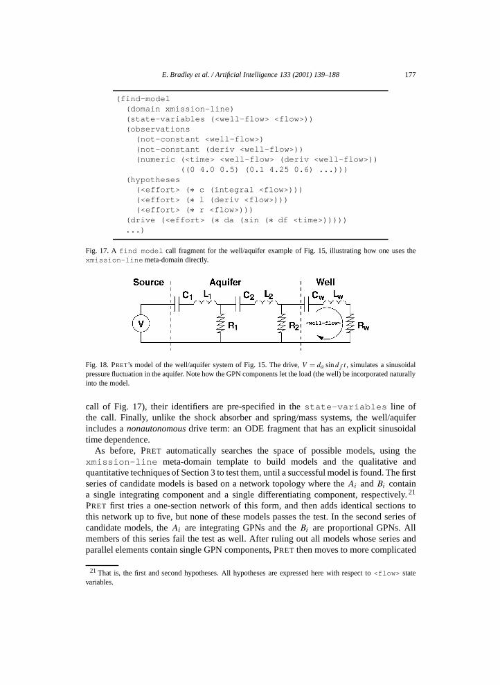
E. Bradley et al. / Artificial Intelligence 133 (2001) 139–188 177
(find-model(domain xmission-line)(state-variables (<well-flow> <flow>))(observations
(not-constant <well-flow>)(not-constant (deriv <well-flow>))(numeric (<time> <well-flow> (deriv <well-flow>))
((0 4.0 0.5) (0.1 4.25 0.6) ...)))(hypotheses
(<effort> (∗ c (integral <flow>)))(<effort> (∗ l (deriv <flow>)))(<effort> (∗ r <flow>)))
(drive (<effort> (∗ da (sin (∗ df <time>)))))...)
Fig. 17. Afind model call fragment for the well/aquifer example of Fig. 15, illustrating how one uses thexmission-linemeta-domain directly.
Fig. 18. PRET’s model of the well/aquifer system of Fig. 15. The drive,V = da sindf t , simulates a sinusoidalpressure fluctuation in the aquifer. Note how the GPN components let the load (the well) be incorporated naturallyinto the model.
call of Fig. 17), their identifiers are pre-specified in thestate-variables line ofthe call. Finally, unlike the shock absorber and spring/mass systems, the well/aquiferincludes anonautonomous drive term: an ODE fragment that has an explicit sinusoidaltime dependence.
As before, PRET automatically searches the space of possible models, using thexmission-line meta-domain template to build models and the qualitative andquantitative techniques of Section 3 to test them, until a successful model is found. The firstseries of candidate models is based on a network topology where theAi andBi containa single integrating component and a single differentiating component, respectively.21
PRET first tries a one-section network of this form, and then adds identical sections tothis network up to five, but none of these models passes the test. In the second series ofcandidate models, theAi are integrating GPNs and theBi are proportional GPNs. Allmembers of this series fail the test as well. After ruling out all models whose series andparallel elements contain single GPN components, PRET then moves to more complicated
21That is, the first and second hypotheses. All hypotheses are expressed here with respect to<flow> statevariables.

178 E. Bradley et al. / Artificial Intelligence 133 (2001) 139–188
topologies. The first such series hasAi as a serial network containing a differentiatingand an integrating GPN component andBi as a single proportional component; the thirdelement of this series, shown in Fig. 18, passes all qualitative and quantitative checks. InPRET’s internal format, this model is expressed as follows:
(= (+ (∗ (deriv (deriv <i1>)) l1)(∗ da (sin (∗ df <time>)))(∗ c1 <i1>) (∗ r1 (deriv <i1>))(- (∗ r1 (deriv <i2>)))) 0)
(= (+ (∗ (deriv (deriv <i2>)) l2) (∗ r1 (deriv <i2>))(- (∗ r1 (deriv <i1>))) (∗ c2 <i2>)(∗ r2 (deriv <i2>))(- (∗ r2 (deriv <iW>)))) 0)
(= (+ (∗ (deriv (deriv <iW>)) lW) (∗ r2 (deriv <iW>))(- (∗ r2 (deriv <i2>))) (∗ cW <iW>)(∗ rW (deriv <iW>))) 0)
A perfect model of a spatiotemporally distributed system, of course, requires an infinitenumber of discrete sections, but one can construct approximations using only a fewsections, and the fidelity of the match rises with the number of sections. This dovetailsneatly with PRET’s specifications, which prescribe the required resolution of themodel: The CBM framework simply keeps adding sections until the model matches theobservations.22 In this case, it used twoxmission-line sections to model the aquiferand one to model the well. This automatic incorporation of the well as an integral partof the model—the rightmost loop in Fig. 15—is an important feature, as loading effectsplay critical roles in engineering analysis and design. The behavior of an audio amplifier,for example, will change radically if one short-circuits its speaker outputs, and the two-terminal GPN load model would factor in those effects automatically. Component-basedmodeling also facilitates a simple and natural treatment of the drive term, which is attacheddirectly to the iterative part of the network. With this approach, an actuator itself, with itsvarious nonlinear and non-ideal properties, is represented directly as part of the network;its effects automatically become part of the model, just as they do in real systems. Finally,like linear-plus, thexmission-line meta-domain lets PRET avoid duplicationof effort. Connecting arbitrary components in parallel and series creates an exponentialnumber of candidate models, many of which are mathematically equivalent (cf., Théveninand Norton equivalents, in network theory). Thexmission-line meta-domain avoidsthis duplication by first limiting the number of possible component combinations in theinitial network model and then incrementing this structure to a limited depth beforeattempting another initial network.
5.3. Modeling a driven pendulum
The driven pendulum introduced in Section 4 is a prototypical example in dynamicalsystems and control theory. It is also widely useful in mechanical engineering in general
22This is exactly the notion of an ODE truncation of a PDE, which PRET uses thexmission-line meta-domain to capture.
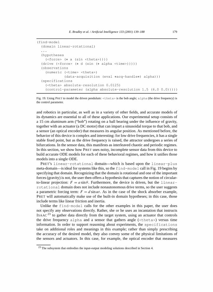
E. Bradley et al. / Artificial Intelligence 133 (2001) 139–188 179
(find-model(domain linear-rotational)...(hypotheses
(<force> (∗ a (sin <theta>))))(drive (<force> (∗ d (sin (∗ alpha <time>)))))(observations
(numeric (<time> <theta>)(data-acquisition (eval ∗acq-handle∗) alpha)))
(specifications(<theta> absolute-resolution 0.0125)(control-parameter (alpha absolute-resolution 1.5 (6.0 0.0)))))
Fig. 19. Using PRET to model the driven pendulum:<theta> is the bob angle;alpha (the drive frequency) isthe control parameter.
and robotics in particular, as well as in a variety of other fields, and accurate models ofits dynamics are essential to all of these applications. Our experimental setup consists ofa 15 cm aluminum arm (“bob”) rotating on a ball bearing under the influence of gravity,together with an actuator (a DC motor) that can impart a sinusoidal torque to that bob, anda sensor (an optical encoder) that measures its angular position. As mentioned before, thebehavior of this device is complex and interesting: for low drive frequencies, it has a singlestable fixed point, but as the drive frequency is raised, the attractor undergoes a series ofbifurcations. In the sensor data, this manifests as interleaved chaotic and periodic regimes.In this section, we show how PRET uses noisy, incomplete sensor data from this device tobuild accurate ODE models for each of these behavioral regimes, and how it unifies thosemodels into a single ODE.
PRET’s linear-rotational domain—which is based upon thelinear-plusmeta-domain—is ideal for systems like this, so thefind-model call in Fig. 19 begins byspecifying that domain. Recognizing that the domain is rotational and one of the importantforces (gravity) is not, the user then offers a hypothesis that captures the notion of circular-to-linear projection:F = a sinθ . Furthermore, the device is driven, but thelinear-rotational domain does not include nonautonomous drive terms, so the user suggestsa parametric forcing term:F = d sinαt . As in the case of the shock absorber example,PRET will automatically make use of the built-in domain hypotheses; in this case, thoseinclude terms like linear friction and inertia.
Unlike the find-model calls for the other examples in this paper, the user doesnot specify any observations directly. Rather, she or he uses an incantation that instructsISAAC 23 to gather data directly from the target system, using an actuator that controlsthe drive frequencyalpha and a sensor that gathers angle (<theta>) versus timeinformation. In order to support reasoning about experiments, thespecificationstake on additional roles and meanings in this example; rather than simply prescribingthe accuracy of the desired model, they also convey some of the physical limitations ofthe sensors and actuators. In this case, for example, the optical encoder that measures
23The subsystem that embodies the input-output modeling solutions described in Section 4.

180 E. Bradley et al. / Artificial Intelligence 133 (2001) 139–188
<theta> has a resolution of± 0.7 degrees. The motor that drives the pendulum has afixed amplitude; its frequency range and resolution are 0–6 radians per second and 1.5radians per second, respectively. This information alone, however, is not enough to letPRET execute experiments automatically. Every sensor and actuator is different—whetherit is digital or analog, voltage- or current-activated, involves frequency or phase, etc.Because this kind of information is all but impossible to deduce automatically, PRET
requires its user to give a minimal description of the operative sensors and actuators, inthe form of a short SCHEME procedure (in this case called∗acq-handle∗) that the userdefines in the environment from which he or she calls PRET. The function, which is used togather data from the target system for specific settings of the parameteralpha, is passed toPRET in thefind-model call via the keywordeval, which causes the variable∗acq-handle∗ to be evaluated in the calling environment. In this case,∗acq-handle∗ hasone argument—the control parameteralpha—and it returns a time series<theta> vs.<time>:
(define ∗acq-handle∗(let ((length 100) ;;; run 100 seconds for
each alpha(time-step 0.1) ;;; sample at 10 Hz(type ’DC-voltage)) ;;; sensor type
(lambda (alpha)(let ((v-control alpha))
(run-DAQ length time-step type v-control)))))
The functionrun-DAQ, which is part of ISAAC’s knowledge base, manages the data-acquisition (DAQ) system that communicates with the actuator and sensor. Its first threearguments specify the length and sample rate of the sensor trace,24 together with thesensor type. (There are currently four types of sensors—AC-voltage, DC-voltage,4-wire-resistance, and4-wire-temperature—and four types of actuators:DC and AC voltage and current sources.)run-DAQ first sends a control voltage (v-control) out to the physical device via the DAQ system’s digital-to-analog converter;this voltage is connected to the frequency-control input of the motor that drives thependulum base. As instructed by∗acq-handle∗, run-DAQ then uses the DAQ’smultimeter board to gather a 100-second long time series of the voltage from the bobangle sensor, measured every tenth of a second. The associated driver function operatesvia system calls to the Standard Instrument Control Library (SICL) [50], which containshigh-level procedures that control the data-acquisition hardware. PRET will eventuallyincorporate a variety of such driver functions, one for each useful actuator/sensorcombination that is supported by the DAQ.
PRET begins by building an ODE model for the first time series. As before, the modelgenerator proposes simple models first and more-complicated ones later, and the model
24Typically, the user will set thetime-step of this sensor trace to be equal to the time resolution in thespecifications section of thefind-model call. However, this is not an absolute requirement. Whereasthetime-step determines the sample rate at which data is gathered, theresolution specifies how closelythe final ODE model must match the data.

E. Bradley et al. / Artificial Intelligence 133 (2001) 139–188 181
tester checks these models individually, always taking advantage of the abstract-reasoning-first paradigm to discard bad models quickly. The qualitative information distilled outof the sensor data during the QBA procedure plays a particularly important role inthis process; without it, the rest of PRET would be forced to rely on manipulations ofthe low-level data in order to build and test models, which is an extremely expensiveproposition. For example, the first step in the delay-coordinate embedding procedureestimates the dimension of the system dynamics; this symbolic fact allows the modeltester to immediately rule out all first-order models. Because the formulae that encodethe information returned by the geometric reasoning processes reside at high abstractionlevels, the logic system can preferentially use this kind of abstract information to establishcontradictions between model and observations quickly and cheaply.
Once PRET accepts a model for the initial time series, ISAAC repeats the reconstruc-tion/classification procedure at the nextalpha value. The∗acq-handle∗ uses theabsolute-resolution range and step specifications in thefind-model call toincrement the control parameteralpha. If the behavior of the resulting time series isqualitatively the same, ISAAC conjectures that the physical system is in the same regimeof the qualitative state/parameter space. Reasoning from this conjecture, the model gener-ator proposes the model that it constructed for the previousalpha value. If, however, theportrait is qualitatively different (e.g., the attractor has undergone a bifurcation), ISAAC as-sumes that the previously identified model does not hold, and so the model search processfor this particular time series must begin anew. PRET continues looping in this fashion untilall of thealpha values have been investigated. If it identifies different models for adja-cent regimes, it attempts to unify the two in a pair-wise fashion—by applying the secondmodel to the first model’s regime and vice versa. Since coefficient values may vary betweenneighboring domains even if the same ODE holds in both, this generally requires anotherround of parameter estimation on each model. Whichever one is applicable in both regimesis accepted as the unifying model. Such a model may not, of course, exist; a system maybe governed by completely different physics in different regimes, and thus no single ODEmay be able to account for its behavior. In such a case, the different regime models wouldbe mutually exclusive and the unification process would be unable to create a single ODE.If this happens, our solution is to simply return the list of regimes, models, and transitions,which is exactly the form of a traditional hybrid model [18] of a multi-regime system.
For the driven pendulum, this procedure plays out as follows:• ISAAC begins its exploration of the system by generating a time series with the drive
frequencyα set to 6.0 radians per second, and its sensor analysis tools identifythe resulting pendulum phase portrait as alimit-cycle response. The modelgenerator proposes a number of first-order models, which the model tester eliminatesusing qualitative and quantitative means. The model generator next proposes asecond-order model using a single built-in domain hypothesis that represents aproportional relationship between force and angular displacement:θ = a1θ . Themodel tester accepts this model with the parameter valuea1=−35.99.• ISAAC continues its exploration at the next control parameter value (α = 4.5) and
again identifies the time series as alimit-cycle. Since the neighboring phaseportraits are qualitatively similar, ISAAC reasons that the adjacent regime’s model isa good starting point, and so it signals the model generator accordingly. In this case,

182 E. Bradley et al. / Artificial Intelligence 133 (2001) 139–188
however, this conjecture is not borne out. Though the phase portraits are qualitativelysimilar, the arc of the pendulum arm is much larger at slower drive frequencies. Thisquantitative difference actually necessitates aqualitative change in the ODE model.In particular, a pendulum may be modeled as a simple harmonic oscillator if the angleis small (θ ≈ sinθ ). At larger angles, however, this approximation no longer holds,so the simple harmonic oscillator (θ = a1θ ) model from the neighboring regime failsthe test, forcing PRET to begin the model search anew. (This is an example of whatwe call an “incorrect” ODE: one whose solutions cannot match the observed timeseries forany coefficient values.) PRET continues generating and testing as before,eventually finding the nonlinear modelθ = a sinθ with a =−36.10. The next step isto reconcile the two models, applying both of them in both regimes. Sinceθ = a sinθsubsumesθ = a1θ , PRET discards the latter.• ISAAC continues the QBA procedure by repeating the reconstruction/classifica-
tion procedure atα = 3.0, finds that the pendulum has bifurcated into a newbehavior regime (in this case, chaotic),25 and again restarts the model search. Aftergenerating and testing several models, PRET finds the ODE modelθ = a2θ+a sinθ+d sinαt , which contains another built-inlinear-rotational domain hypothesisthat relates force and angularvelocity, with coefficient valuesa2 = −1.65, a =−24.81, d = 20.72, andα = 3.02. (This is actually the globally valid model, butPRET cannot know this and must treat it as any other.) Note that theα value in thismodel is not exactly 3.000. This comes about because PRET’s parameter estimatoradjusts the model coefficients to optimize its fit to the observed time series—anintentional design feature that lets it ignore any noise that may be present in itsboundary conditions. Lastly, PRET notes that this more-complex model subsumes theneighboring regime’s model (θ = a sinθ ), and so accepts the former in both regimes;at the same time, it performs a bisecting search to find the preciseα value for theboundary between them.• At the nextalpha value, 1.5, ISAAC identifies the phase portrait as alimit-cycle. Since this behavior has been observed before, ISAAC has examples fromwhich to work. In particular, it proposes the most recent model that was valid in alimit-cycle regime—in this case, the globally valid model. The model tester quicklyacceptsθ = a2θ +a sinθ +d sinαt for this regime as well, with the coefficient valuesa2=−1.66, a =−24.49, d = 20.833, andα = 1.50.• At the final control parameter value,α = 0.0, ISAAC identifies the phase portrait as
a damped-oscillation. Since PRET has not yet modeled any such behavior,ISAAC has no prior model to suggest, and the model generator must start anew. Afterrejecting a few models, the model tester acceptsθ = a2θ + a sinθ with a2 =−1.59anda =−24.38. A final unification step accepts the globally valid for this regime aswell.
25This algorithm may miss bifurcations altogether if two or more of them occurbetween parameter slices,canceling out each others’ effects. It is, however, a good compromise; bifurcations represent deep changes inthe dynamics, and each one leaves a highly individual signature in the behavior—signatures that are unlikely tocancel out.

E. Bradley et al. / Artificial Intelligence 133 (2001) 139–188 183
Table 3Models of the driven pendulum in different behavioral regimes
Drive ODE Description
Frequency
None θ (t)= a2θ (t)+ a sinθ(t) Damped oscillator
Low θ (t)= a2θ (t)+ a sinθ(t)+ d1 sinαt Complex oscillator
Medium θ (t)= a2θ (t)+ a sinθ(t)+ d1 sinαt Chaotic behavior
High θ (t)= a sinθ(t) Sinusoidal oscillator
Very High θ (t)= a1θ(t) Small angle (linear) model
In the absence of unification, PRET would return different ODE models, listed in Table 3,for the five different regimes that ISAAC identifies in this system. Because it interleaves theunification process with the model-building process, however, PRET is able to unify thesemodels in a straightforward and efficient manner. Even more important, this interleavingcan vastly reduce the complexity of the generate phase. One problem with the pair-wiseunification procedure, however, is that it can fail to unify a set of models even if it includesa single globally valid one. For example, assume model “A” is discovered first, followed bya different model “B” and that these two models cannot be unified. If a third and globallyunifying model “C” is found next, the pair-wise procedure would not correctly unify thethree models into one. A better unification procedure that solves the pair-wise deficiencywould be to apply all valid models to every time series. We choose not to do this because itis expensive—O(n2), wheren is the number of time series—and not absolutely necessary;practicing engineers are quite capable of deciding which models in a list subsume oneanother if PRET misses a few equivalences.
6. Conclusion
PRET is designed to produce the type of formal engineering models that a humanexpert would create—quickly and automatically. Unlike existing system identificationtools, PRET is not just a fancy parameter estimator; rather, it uses sophisticated knowledgerepresentation and reasoning techniques to automate the structural identification phase ofmodel building as well. Unlike existing AI tools, PRET takes anactive approach to thetask of modeling complex, nonlinear systems, using techniques drawn from engineering,dynamical systems, and control theory to explore their behavior directly, via sensorsand actuators. Unlike any existing software tools, PRET works with high-dimensional,nonlinear, grey-box systems: the kinds of hard problems with which engineers are facedon a daily basis.
The challenges involved in automating nonlinear system identification are significant,especially because PRET is designed to be easily extensible to any problem domainthat admits ordinary differential equations. The control-theoretic issues involved inreasoning about nonlinear dynamical systems—particularly those involving the planningand execution of experiments—routinely stymie human experts. PRET’s solution is based

184 E. Bradley et al. / Artificial Intelligence 133 (2001) 139–188
on two paradigms: generate-and-test and input/output modeling. The generate phase restson a flexible, powerful representation—the generalized physical network—and a layeredhierarchy of knowledge representations that we termdomains and meta-domains. Thisframework lets PRET effectively model systems in a wide variety of application areas andalso adapt smoothly to different levels of domain knowledge. The test phase is based ona first-order logic inference system that uses a variety of heterogeneous reasoning modesto check models against observations. This inference system orchestrates the selection,invocation, and interaction of these reasoning modes using declaratively representedknowledge about dynamical systems, together with knowledge abouthow to reason aboutdynamical systems, in order to test candidate models as cheaply as possible. Input/outputtechniques—automatic planning, execution, and interpretation of experiments—make themodeling process interactive. This is a particularly difficult problem. In practice, onecan rarely measure (or evenknow) all the state variables of a system; usually, one hasaccess to imprecise, noisy sensors attached to some subset of its outputs. PRET works withimprecision by representing and reasoning with it explicitly, deals with noise by QR-guidedfiltering in its nonlinear parameter estimation reasoner, reconstructs any unmeasureddynamics using delay-coordinate embedding, and identifies different behavioral regimesand the connection between inputs and outputs using cell dynamics, bifurcation analysis,and a new representation called the qualitative state/parameter space.
Theoretically, PRET can modelany system that admits an ODE model—even in themost severe black-box situation, where it knows nothing whatsoever about that system.26
Because thexmission-line meta-domain allows PRET to use its lumped-elementGPN components to model spatially distributed systems, it can even model systems thattechnically require PDE models. In practice, however, the size of the associated searchspace and the available computer power limit PRET’s range. The representation andreasoning tactics described in this paper mitigate this by intelligently streamlining themodel-building and -testing processes. Thanks to these tactics, PRET has been able tosuccessfully construct models of a dozen or so textbook problems (Rössler, Lorenz, simplependulum, pendulum on a spring, etc.; see [16,17,34]), as well as several interesting anddifficult real-world examples, such as the well, shock absorber, and driven pendulum inthe previous section and a commercial radio-controlled car, which is covered in [16].These examples are representative of wide classes of dynamical systems, both linear andnonlinear. PRET’s model of the radio-controlled car was particularly interesting; it not onlyfit the experimental data, but actually enabled the project analysts to identify what waswrong with their mental models of the system. Specifically, PRET’s model matched theobservationsbut not their intuition, and the disparities led them to understand the systemdynamics better.
This anecdote brings out an important point: PRET is intended to be an engineer’s tool,and that goal dictated a specific set of design choices. From an engineering standpoint, asuccessful model balances accuracy and parsimony. Accordingly, PRET’s goal is not to in-fer physics that the user left implicit, but rather to construct the simplest model that matchesthe observed behavior to within the predefinedspecifications. Because evaluation
26This is due largely to its Taylor-series model-generation facilities and the lowest-level layer of model-testingtools in Table 2.

E. Bradley et al. / Artificial Intelligence 133 (2001) 139–188 185
criteria are always domain-specific, we believe that modeling tools should let their domain-expert users dictate them, and not simply build in an arbitrary set of thresholds and percent-ages. The notion of aminimal model that is tightly (some might say myopically) guided byits user’s specifications represents a very different philosophy from traditional AI work inthis area. Unlike some scientific discovery systems, PRET makes no attempt to exceed therange and resolution specifications that are prescribed by its user: a loosespecifica-tion for a particular state variable, for instance, is taken as an explicit statement that anexact fit of that state variable is not important to the user, so PRET will not add terms to theODE in order to model small fluctuations in that variable. Conversely, a single out-of-rangedata point will cause a candidate model to fail PRET’s test. These are not unwelcome sideeffects of the finite resolution; they are intentional and useful by-products of the abstrac-tion level of the modeling process. A single outlying data point may appear benign if onereasons only about variances and means, but engineers care deeply about such single-pointfailures (such as the temperature dependence of O-ring behavior in space shuttle boosters),and a tool designed to support such reasoning must reflect those constraints.
Achieving model parsimony and accuracy in the face of incomplete, heterogeneousknowledge and an exponential search space is a nontrivial problem. Automatic planning,execution, and interpretation of experiments can aid in its solution, but the associatedimplementation issues are nontrivial. Manipulating actuators and sensors in order toaugment a model-builder’s knowledge in useful ways is made difficult not only by thecontrol-theoretic issues that are buried in the physics, but also by the meta-knowledgeconstraints that are inherent in the problem requirements. Corroborating, verifying, andeven filling in a human expert’s knowledge is a worthwhile goal, but it can conflictwith model minimality. Nonetheless, automating the input/output modeling process is animportant step for autonomous situations, for nonexpert users, etc., so sensible ways aroundthis conundrum are one of the current foci of our research.
Acknowledgements
Apollo Hogan, Brian LaMacchia, Abbie O’Gallagher, Janet Rogers, Ray Spiteri, andTom Wrensch contributed code and/or ideas to PRET.
References
[1] H. Abarbanel, Analysis of Observed Chaotic Data, Springer, Berlin, 1995.[2] H. Abelson, The bifurcation interpreter: A step towards the automatic analysis of dynamical systems,
Internat. J. Comput. Math. Appl. 20 (1990) 13.[3] S. Addanki, R. Cremonini, J.S. Penberthy, Graphs of models, Artificial Intelligence 51 (1991) 145–178.[4] J. Amsterdam, Automated qualitative modeling of dynamic physical systems, Ph.D. Thesis, MIT,
Cambridge, MA, 1992.[5] K. Astrom, P. Eykhoff, System identification—A survey, Automatica 7 (1971) 123–167.[6] A. Barrett, D. Christianson, M. Friedman, C. Kwok, K. Golden, S. Penberthy, Y. Sun, D. Weld,
UCPOP User’s Manual (version 4.0), Technical Report 93-09-06d, Department of Computer Science andEngineering, University of Washington, Seattle, WA, 1995.
[7] C. Beckstein, R. Stolle, G. Tobermann, Meta-programming for generalized Horn clause logic, in: Proc. 5thInternational Workshop on Metaprogramming, Metareasoning in Logic (META-96), Bonn, Germany, 1996,pp. 27–42.

186 E. Bradley et al. / Artificial Intelligence 133 (2001) 139–188
[8] C. Beckstein, G. Tobermann, Evolutionary logic programming with RISC, in: Proc. 4th InternationalWorkshop on Logic Programming Environments, Washington, DC, Technical Report TR 92-143, Centerfor Automation and Intelligent Systems Research at Case Western Reserve University, Cleveland, OH,November 1992, pp. 16–21.
[9] C. Beckstein, G. Tobermann, Algorithmic debugging and hypothetical reasoning, J. Automat. SoftwareEngineering 4 (1997) 151–178.
[10] F. Besinger, D. Cebon, D. Cole, Damper models for heavy vehicle ride dynamics, Vehicle SystemDynamics 24 (1997) 35–64.
[11] P. Boggs, R. Byrd, J. Rogers, R. Schnabel, User’s reference guide forODRPACK—Software for weightedorthogonal distance regression, Technical Report 4103, National Institute of Standards and Technology,Gaithersburg, MD, 20899, 1991.
[12] P. Boggs, R. Byrd, R. Schnabel, A stable and efficient algorithm for nonlinear orthogonal distanceregression, SIAM J. Sci. Statist. Comput. 8 (6) (1987) 1052–1078.
[13] E. Bradley, Autonomous exploration and control of chaotic systems, Cybernetics and Systems 26 (1995)299–319.
[14] E. Bradley, Time-series analysis, in: M. Berthold, D. Hand (Eds.), Intelligent Data Analysis: AnIntroduction, Springer, Berlin, 2000.
[15] E. Bradley, M. Easley, Reasoning about sensor data for automated system identification, Intelligent DataAnalysis 2 (2) (1998) 123–138.
[16] E. Bradley, A. O’Gallagher, J. Rogers, Global solutions for nonlinear systems using qualitative reasoning,Ann. Math. Artificial Intelligence 23 (1998) 211–228.
[17] E. Bradley, R. Stolle, Automatic construction of accurate models of physical systems, Ann. Math. ArtificialIntelligence 17 (1996) 1–28.
[18] M. Branicky, V. Borkar, S. Mitter, A unified framework for hybrid control, in: Proc. 33rd IEEE Conferenceon Decision & Control, Lake Buena Vista, FL, 1994, pp. 4228–4234.
[19] J. Bredehoeft, H. Cooper, I. Papadopulos, Inertial and storage effects in well-aquifer systems, WaterResource Research 2 (4) (1966) 697–707.
[20] W. Brogan, Modern Control Theory, 3rd edn., Prentice-Hall, Englewood Cliffs, NJ, 1991.[21] A. Capelo, L. Ironi, S. Tentoni, Automated mathematical modeling from experimental data: An application
to material science, IEEE Trans. Systems Man Cybernet. 28 (1998) 356–370.[22] J. Carbonell, J. Blythe, O. Etzioni, Y. Gil, R. Joseph, D. Kahn, C. Knoblock, S. Minton, A. Pérez, S. Reilly,
M. Veloso, X. Wang, PRODIGY 4.0: The manual and tutorial, Technical Report CMU-CS-92-150, Schoolof Computer Science, Carnegie Mellon University, Pittsburgh, PA, 1992.
[23] B.W. Char, K.O. Geddes, G.H. Gonnet, B.L. Leong, M.B. Monagan, S.M. Watt, Maple V LanguageReference Manual, Springer, Berlin, 1991.
[24] M. Cherniack, S. Zdonik, Changing the rules: Transformations for rule-based optimizers, in: Proc. ACMSIGMOD International Conference on Management of Data, Seattle, WA, 1998.
[25] D. Chin, Water-Resource Engineering, Prentice Hall, Englewood Cliffs, NJ, 2000.[26] R. Davis, Meta-rules: Reasoning about control, Artificial Intelligence 15 (3) (1980) 179–222.[27] J. de Kleer, An assumption-based TMS, Artificial Intelligence 28 (2) (1986) 127–162.[28] J. de Kleer, B.C. Williams (Eds.), Artificial Intelligence, Vol. 51, Elsevier Science, Amsterdam, 1991,
Special Volume on Qualitative Reasoning about Physical Systems II.[29] D. D’Humieres, M. Beasley, B. Huberman, A. Libchaber, Chaotic states and routes to chaos in the forced
pendulum, Phys. Rev. A 26 (1982) 3483–3496.[30] S. Džeroski, L. Todorovski, Discovering dynamics: From inductive logic programming to machine
discovery, J. Intelligent Inform. Systems 4 (1995) 89–108.[31] M. Easley, Automating input-output modeling of dynamic physical systems, Ph.D. Thesis, University of
Colorado at Boulder, 2000.[32] M. Easley, E. Bradley, Generalized physical networks for model building, in: Proc. IJCAI-99, Stockholm,
Sweden, 1999, pp. 1047–1052.[33] M. Easley, E. Bradley, Reasoning about input-output modeling of dynamical systems, in: Proc. 3rd
International Symposium on Intelligent Data Analysis (IDA-99), Amsterdam, Springer, Berlin, 1999,pp. 343–355.
E. Bradley et al. / Artificial Intelligence 133 (2001) 139–188 187
[34] M. Easley, E. Bradley, Meta-domains for automated system identification, in: C.H. Dagli, M. Akay,O.K. Ersoy, Ferná, A. Smith (Eds.), Proc. Smart Engineering System Design (ANNIE 00), ASME Press,Fairfield, NJ, 2000, pp. 165–170.
[35] J. Everett, K. Forbus, Scaling up logic-based truth maintenance systems via fact garbage collection, in: Proc.AAAI-96, Portland, OR, 1996, pp. 614–620.
[36] B. Falkenhainer, K. Forbus, Compositional modeling: Finding the right model for the job, ArtificialIntelligence 51 (1991) 95–143.
[37] B. Faltings, E. Gelle, Local consistency for ternary numeric constraints, in: Proc. IJCAI-97, Nagoya, Japan,1997, pp. 392–397.
[38] B. Faltings, P. Struss (Eds.), Recent Advances in Qualitative Physics, MIT Press, Cambridge, MA, 1992.[39] K. Forbus, Qualitative process theory, Artificial Intelligence 24 (1984) 85–168.[40] K. Forbus, Interpreting observations of physical systems, IEEE Trans. Systems Man Cybernet. 17 (3) (1987)
350–359.[41] K. Forbus, Qualitative reasoning, in: A. Tucker (Ed.), CRC Computer Science and Engineering Handbook,
CRC Press, Boca Raton, FL, 1997.[42] J. Forrester, World Dynamics, Wright Allen Press, New York, 1971.[43] D.M. Gabbay, M.J. Sergot, Negation as inconsistency I, J. Logic Programming 3 (1) (1986) 1–36.[44] H. Gallaire, C. Lasserre, Controlling knowledge deduction in a declarative approach, in: Proc. IJCAI-79,
Tokyo, Japan, 1979, pp. S–1–S–6.[45] H. Gallaire, C. Lasserre, Metalevel control for logic programs, in: K.L. Clark, S.A. Tärnlund (Eds.), Logic
Programming, Academic Press, London, 1982, pp. 173–185.[46] H. Goldstein, Classical Mechanics, Addison Wesley, Reading, MA, 1980.[47] B. Grosof, Courteous logic programs: Prioritized conflict handling for rules, Technical Report RC 20836,
IBM Research, 1997.[48] J. Halling (Ed.), Principles of Tribology, MacMillan, 1978.[49] B. Hannon, M. Ruth, Dynamic Modeling, Springer, New York, 1995.[50] Hewlett-Packard, Standard Instrument Control Library Reference Manual, 1996.[51] P. Hill, J. Lloyd, The Gödel Programming Language, MIT Press, Cambridge, MA, 1994.[52] A. Hogan, R. Stolle, E. Bradley, Putting declarative meta control to work. Technical Report CU-CS-856-98,
University of Colorado at Boulder, 1998.[53] D. Hong, S. Velinsky, X. Feng, Verification of a wheeled mobile robot dynamic model and control
ramifications, Dynamic Systems, Measurement, and Control 131 (1) (1999) 58–63.[54] R. Horst, P. Pardalos, N. Thoai, Introduction to Global Optimization, Nonconvex Optimization and its
Applications, Vol. 3, Kluwer, Dordrecht, 1987.[55] C. Hsu, A theory of cell-to-cell mapping dynamical systems, J. Appl. Mech. 47 (1980) 931–939.[56] C. Hsu, Cell-to-Cell Mapping, Springer, New York, 1987.[57] K.-M. Huang, J.M. Zytkow, Discovering empirical equations from robot-collected data, in: Z. Ras,
A. Skowron (Eds.), Foundations of Intelligent Systems, Lecture Notes in Computer Science, Vol. 1325,Springer, Berlin, 1997, pp. 287–297. Proceedings of ISMIS-97, Charlotte, NC, October 1997.
[58] J. Jaffar, M. Maher, Constraint logic programming: A survey, J. Logic Programming 20 (1994) 503–581.[59] J.-N. Juang, Applied System Identification, Prentice Hall, Englewood Cliffs, NJ, 1994.[60] D. Karnopp, D. Margolis, R. Rosenberg, System Dynamics: A Unified Approach, 2nd edn., Wiley, New
York, 1990.[61] B.J. Kuipers, Qualitative simulation, Artificial Intelligence 29 (3) (1986) 289–338.[62] B.J. Kuipers, Qualitative Reasoning: Modeling and Simulation with Incomplete Knowledge, Addison-
Wesley, Reading, MA, 1992.[63] P. Langley, H.A. Simon, G.L. Bradshaw, J.M. Zytkow (Eds.), Scientific Discovery: Computational
Explorations of the Creative Process, MIT Press, Cambridge, MA, 1987.[64] R. Langlois, R. Anderson, Preview control algorithms for the active suspension of an off-road vehicle,
Vehicle System Dynamics 24 (1997) 65–97.[65] J. LeFèvre, Reactive system dynamics: An extension of forrester’s system dynamics using bond graph-like
notations, in: Bond Graph Modeling and Simulations, ICBGM ’97, Conference Proceedings, Phoenix, AZ,1997, pp. 149–155.
[66] L. Ljung (Ed.), System Identification: Theory for the User, Prentice-Hall, Englewood Cliffs, NJ, 1987.

188 E. Bradley et al. / Artificial Intelligence 133 (2001) 139–188
[67] J.W. Lloyd, Foundations of Logic Programming, 2nd extended edn., Springer, Berlin, 1987.[68] L. McCarty, Clausal intuitionistic logic I. Fixed-point semantics, J. Logic Programming 5 (1988) 1–31.[69] F. Morrison, The Art of Modeling Dynamic Systems, Wiley, New York, 1991.[70] P. Mosterman, G. Biswas, Formal specifications for hybrid dynamical systems, in: Proc. IJCAI-97, Nagoya,
Japan, 1997.[71] P.J. Mosterman, G. Biswas, A formal hybrid modeling scheme for handling discontinuities in physical
system models, in: Proc. AAAI-96, Portland, OR, 1996, pp. 985–990.[72] N. Muscettola, P. Nayak, B. Pell, B. Williams, Remote agent: To boldly go where no AI system has gone
before, Artificial Intelligence 103 (1998) 5–48.[73] P.P. Nayak, Automated Modeling of Physical Systems, Lecture Notes in Computer Science, Vol. 1003,
Springer, Berlin, 1995. Revised version of Ph.D. Thesis, Stanford University, 1992.[74] H. Paynter, Analysis and Design of Engineering Systems, MIT Press, Cambridge, MA, 1961.[75] J. Rees, W. Clinger, The revised3 report on the algorithmic language Scheme, ACM SIGPLAN Notices 21
(1986) 37.[76] J. Reid, Linear System Fundamentals, McGraw-Hill, New York, 1983.[77] V. Robins, J. Meiss, E. Bradley, Computing connectedness: An exercise in computational topology,
Nonlinearity 11 (1998) 913–922.[78] V. Robins, J. Meiss, E. Bradley, Computing connectedness: Disconnectedness and discreteness, Physica
D 139 (2000) 276–300.[79] R. Sanford, Physical Networks, Prentice-Hall, Englewood Cliffs, NJ, 1965.[80] T. Sauer, J. Yorke, M. Casdagli, Embedology, J. Statist. Phys. 65 (1991) 579–616.[81] E.D. Sontag, Mathematical Control Theory, Springer, Berlin, 1998.[82] L. Sterling, E. Shapiro, The Art of PROLOG, MIT Press, Cambridge, MA, 1986.[83] R. Stolle, Integrated multimodal reasoning for modeling of physical systems, Ph.D. Thesis, University of
Colorado, 1998. To appear in Lecture Notes in Computer Science, Springer, Berlin.[84] R. Stolle, E. Bradley, A customized logic paradigm for reasoning about models, in: Y. Iwasaki, A. Farquhar
(Eds.), Proc. 10th International Workshop on Qualitative Reasoning (QR-96), Stanford Sierra Camp, CA,AAAI Technical Report WS-96-01, 1996.
[85] R. Stolle, E. Bradley, Multimodal reasoning for automatic model construction, in: Proc. AAAI-98, Madison,WI, 1998, pp. 181–188.
[86] S. Strogatz, Nonlinear Dynamics and Chaos, Addison-Wesley, Reading, MA, 1994.[87] G. Sussman, G. Steele, CONSTRAINTS—A language for expressing almost hierarchical descriptions,
Artificial Intelligence 14 (1980) 1–39.[88] L. Todorovski, S. Džeroski, Declarative bias in equation discovery, in: Proc. 14th International Conference
on Machine Learning (ICML-97), San Francisco, CA, Morgan Kaufmann, San Mateo, CA, 1997, pp. 376–384.
[89] J. Top, H. Akkermans, Computational and physical causality, in: Proc. IJACI-91, Sydney, Australia, 1991.[90] A. Torn, A. Zilinskas, Global Optimization, Lecture Notes in Computer Science, Vol. 350, Springer, Berlin,
1995.[91] T. Washio, H. Motoda, N. Yuji, Discovering admissible model equations from observed data based on scale-
types and identity constraints, in: Proc. IJCAI-99, Stockholm, Sweden, 1999, pp. 772–779.[92] D. Weld, J. de Kleer (Eds.), Readings in Qualitative Reasoning about Physical Systems, Morgan Kaufmann,
San Mateo, CA, 1990.[93] D.S. Weld, Reasoning about model accuracy, Artificial Intelligence 56 (1992) 255–300.[94] B.C. Williams, W. Millar, Decompositional, model-based learning and its analogy to diagnosis, in: Proc.
AAAI-98, Madison, WI, 1998.[95] K. Yip, KAM: A System for Intelligently Guiding Numerical Experimentation by Computer, Artificial
Intelligence Series, MIT Press, Cambridge, MA, 1991.[96] F. Zhao, Computational dynamics: Modeling and visualizing trajectory flows in phase space, Ann. Math.
Artificial Intelligence 8 (1993) 285–300.[97] J.M. Zytkow, Model construction: Elements of a computational mechanism, in: Proc. Conference on
Creativity, Edinburgh, 1999.


![Active Learning for Nonlinear System Identification with ...arXiv:2006.10277v1 [stat.ML] 18 Jun 2020 Active Learning for Nonlinear System Identification with Guarantees Horia Mania](https://img.pdfslide.us/doc/110x75/60d4813c8eceea7d64273b88/active-learning-for-nonlinear-system-identiication-with-arxiv200610277v1.jpg)
![Sparse Identification of Nonlinear Dynamical …arXiv:2005.13232v1 [stat.ML] 27 May 2020 Sparse Identification of Nonlinear Dynamical Systems via Reweighted ℓ1-regularized Least](https://img.pdfslide.us/doc/110x75/5fbe8824ad344c04ec197bab/sparse-identification-of-nonlinear-dynamical-arxiv200513232v1-statml-27-may.jpg)