Embed Size (px)
Citation preview
REALSIMPLE Basic Virtual Acoustic Guitar Lab
Nelson Lee and Julius O. Smith III
RealSimple Project∗
Center for Computer Research in Music and Acoustics (CCRMA)Department of Music, Stanford University
Stanford, California 94305
June 5, 2008
Abstract
This is the REALSIMPLE lab on estimating parameters for a physics-based guitar modelfrom measurements from your own guitar! We discuss various components of a physics-basedmodel, and methods for measuring these components and estimating parameters for correspond-ing model components.
1 Introduction
As discussed in previous labs, there are three components to a phyicals-based guitar model: the exci-tation, the string and the body. The string model, as reviewed in Electric Guitar Lecture: Simple Strings,is based on the Digital Waveguide: a digital implementation of the solution to the Wave Equation.The body of the guitar is implemented as a filter, which can be measured by striking the bridgeof your guitar with an impulse-force hammer. Lastly, we present simple methods for computingexcitation signals to drive your string-model.
2 Setting Up
In this laboratory you will estimate parameters for a physical-model guitar model based on mea-surements of a real acoustic guitar.
Below are the steps to be taken, along with some illustrations of the kind of results you shouldexpect:1
2.1 Required Software
1. Matlab: Student versions of Matlab are available; the Signal Processing Toolbox is required.
2. CCRMA STK (C++ signal toolkit): the STK is free for download from the CCRMA home-page.
∗Work supported by the Wallenberg Global Learning Network1The figures in this laboratory were generated by Stanford Ph.D. student Nelson Lee, using software developed in
the course of his thesis research.
1
2.2 Required Hardware
1. Your guitar!
2. The guitar we used for this lab is a Selmer-Maccaferri copy, similar to the guitar DjangoReinhardt used throughout his career.
3. Our recording setup at CCRMA consisted of a Digidesign M-box 2, with two XLR inputjacks, and Digidesign’s recording software, Pro Tools 7.0. The guitar was equipped with aSchertler DYN-G contact pickup that connected straight into the M-box.
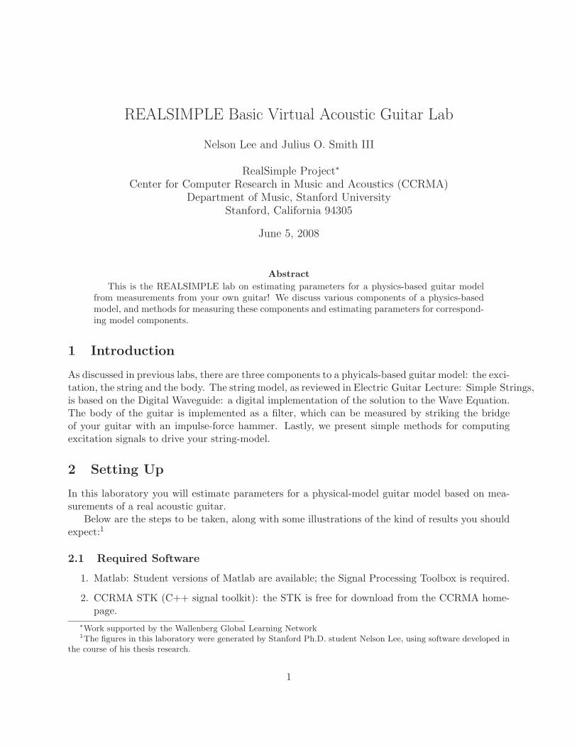
3 Record a Note From Your Guitar
Record a note on your guitar. Figure 1 shows what your note might look like when plotted in thetime domain (highest open note on an acoustic steel-string manouche guitar).
0 1 2 3 4 5 6 7 8−0.06
−0.04
−0.02
0
0.02
0.04
0.06
0.08
0.1
0.12
0.14
seconds
ampl
itude
original signal in time domain
Figure 1: Original signal in the time domain.
The following code segments shows basic usage of reading a file into Matlab and plotting thedata to obtain the results in Figure 1.
2

fileName = ’hard_long_1_16b.wav’;
[y,fs,bits]=wavread(fileName);
%% fs is the sampling rate of the recording
%% here we have fs = 44100
t=(0:length(y)-1)*1/fs;
figure;plot(t,y)
xlabel(’seconds’);
ylabel(’amplitude’);
title(’original signal in time domain’);
3
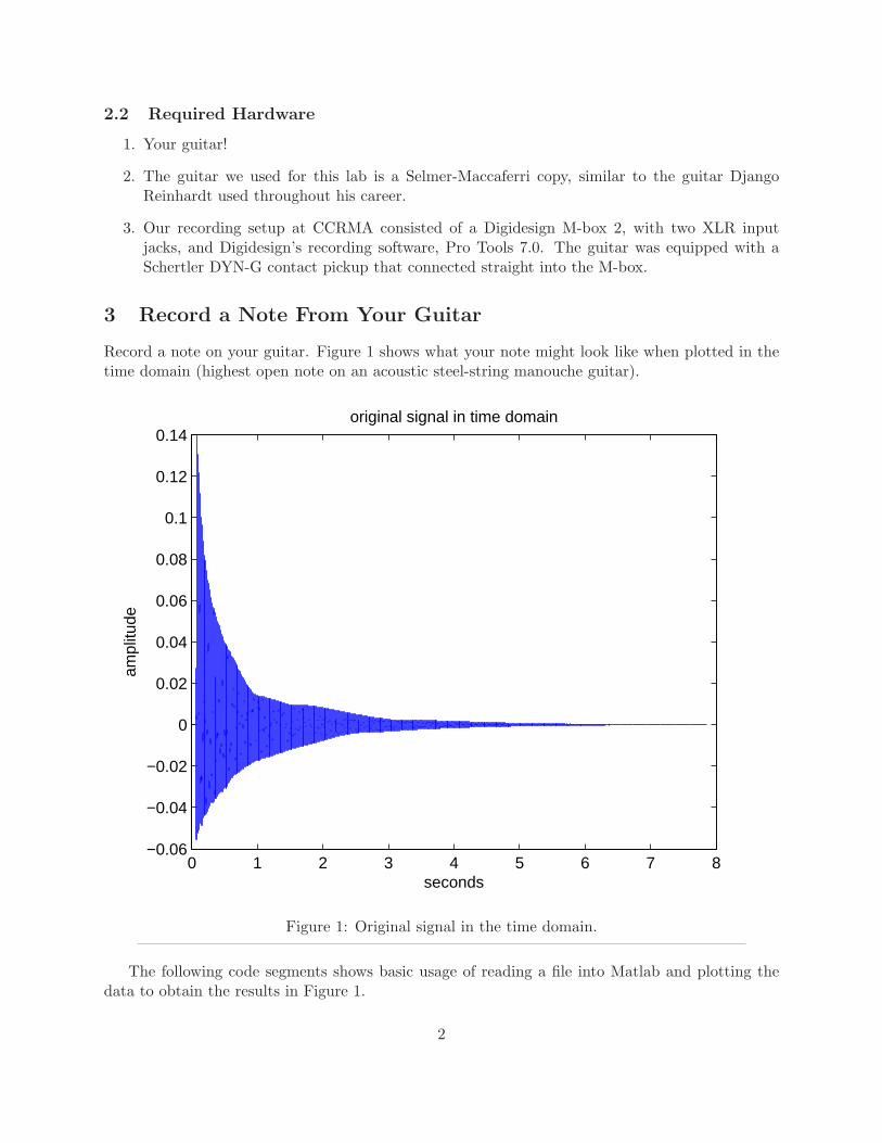
4 The String Model
In this section, we will use a metric commonly used in reverberation studies for estimating thedecay-rates/loop-filter parameters of your string model. The metric, Energy Decay Relief, showshow the energy of a signal decays over time for different frequencies. In this section we will reviewthe Energy Decay Relief and then estimate parameters for your loop filter for your string-model.
4.1 Using the Energy Decay Relief (EDR)
Compute the Energy Decay Relief (EDR) [1] of the original signal. Here we use Matlab’s SignalProcessing Toolkit. The function spectrogram computes the Short-Time Fourier Transform (STFT)of the signal. From the STFT, we compute the EDR. Figure 2 and Fig. 3 show EDRs for the recordednote.
Figure 2: EDR of the signal truncated at -85 dB
We’ve provided the following code segments to demonstrate usage of the Signal ProcessingToolbox in Matlab, as well as three-dimensional plotting.
frameSizeMS = 30; % minimum frame length, in ms
4
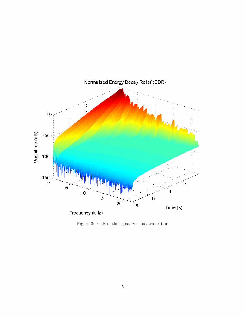
Figure 3: EDR of the signal without truncation
5
overlap = 0.75; % fraction of frame overlapping
windowType = ’hann’; % type of windowing used for each frame
[signal,fs,bits] = wavread(fileName);
% calculate STFT frames
minFrameLen = fs*frameSizeMS/1000;
frameLenPow = nextpow2(minFrameLen);
frameLen = 2^frameLenPow; % frame length = fft size
eval([’frameWindow = ’ windowType ’(frameLen);’]);
[B,F,T] = spectrogram(signal,frameWindow,overlap*frameLen,2*STFT_Npt,fs);
[nBins,nFrames] = size(B);
B_energy = B.*conj(B);
B_EDR = zeros(nBins,nFrames);
for i=1:nBins
B_EDR(i,:) = fliplr(cumsum(fliplr(B_energy(i,:))));
end
B_EDRdb = 10*log10(abs(B_EDR));
% normalize EDR to 0 dB and truncate the plot below a given dB threshold
offset = max(max(B_EDRdb));
B_EDRdbN = B_EDRdb-offset;
B_EDRdbN_trunc = B_EDRdbN;
for i=1:nFrames
I = find(B_EDRdbN(:,i) < minPlotDB);
if (I)
B_EDRdbN_trunc(I,i) = minPlotDB;
end
end
figure(gcf);clf;
mesh(T,F/1000,B_EDRdbN_trunc);
view(130,30);
title(’Normalized Energy Decay Relief (EDR)’);
xlabel(’Time (s)’);ylabel(’Frequency (kHz)’);zlabel(’Magnitude (dB)’);
axis tight;zoom on;
6
4.2 Designing the loop filter for your guitar model
In this section we review Matlab calls for fitting filters to wanted magnitude responses. As usingsuch functions are not only useful for computing the loop-filter of your string-model, it should bekept in mind that such methods are useful for general applications requiring filter-fitting.
4.2.1 Fitting Filters in Matlab
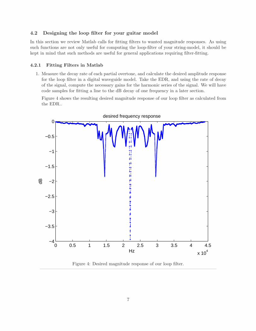
1. Measure the decay rate of each partial overtone, and calculate the desired amplitude responsefor the loop filter in a digital waveguide model. Take the EDR, and using the rate of decayof the signal, compute the necessary gains for the harmonic series of the signal. We will havecode samples for fitting a line to the dB decay of one frequency in a later section.
Figure 4 shows the resulting desired magnitude response of our loop filter as calculated fromthe EDR..
0 0.5 1 1.5 2 2.5 3 3.5 4 4.5
x 104
−4
−3.5
−3
−2.5
−2
−1.5
−1
−0.5
0
dB
Hz
desired frequency response
Figure 4: Desired magnitude response of our loop filter.
7
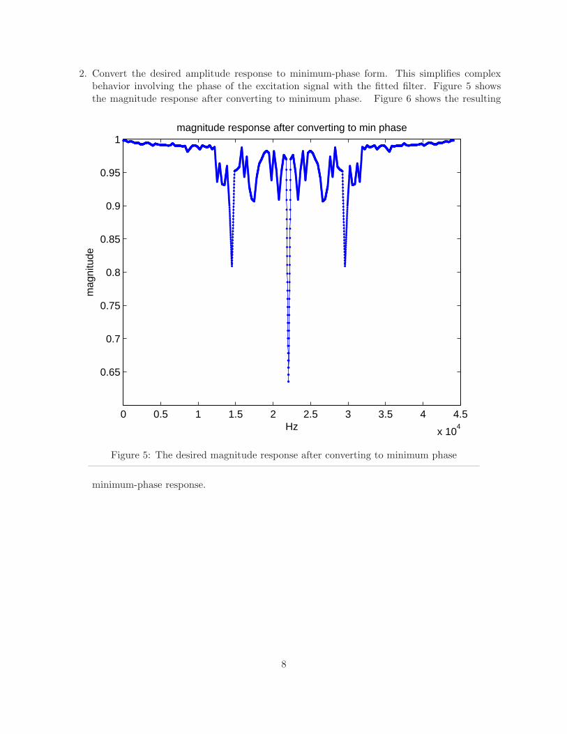
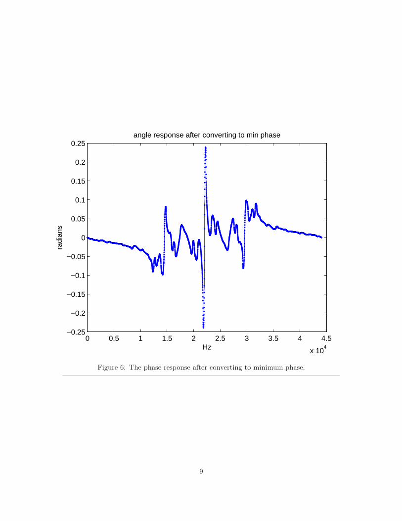
2. Convert the desired amplitude response to minimum-phase form. This simplifies complexbehavior involving the phase of the excitation signal with the fitted filter. Figure 5 showsthe magnitude response after converting to minimum phase. Figure 6 shows the resulting
0 0.5 1 1.5 2 2.5 3 3.5 4 4.5
x 104
0.65
0.7
0.75
0.8
0.85
0.9
0.95
1
mag
nitu
de
Hz
magnitude response after converting to min phase
Figure 5: The desired magnitude response after converting to minimum phase
minimum-phase response.
8
0 0.5 1 1.5 2 2.5 3 3.5 4 4.5
x 104
−0.25
−0.2
−0.15
−0.1
−0.05
0
0.05
0.1
0.15
0.2
0.25
radi
ans
Hz
angle response after converting to min phase
Figure 6: The phase response after converting to minimum phase.
9
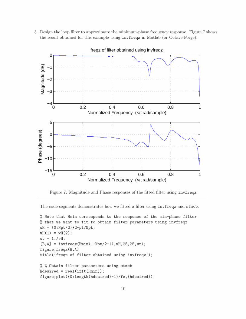
3. Design the loop filter to approximate the minimum-phase frequency response. Figure 7 showsthe result obtained for this example using invfreqz in Matlab (or Octave Forge).
0 0.2 0.4 0.6 0.8 1−15
−10
−5
0
5
Normalized Frequency (×π rad/sample)
Pha
se (
degr
ees)
0 0.2 0.4 0.6 0.8 1−4
−3
−2
−1
0
Normalized Frequency (×π rad/sample)
Mag
nitu
de (
dB)
freqz of filter obtained using invfreqz
Figure 7: Magnitude and Phase responses of the fitted filter using invfreqz
The code segments demonstrates how we fitted a filter using invfreqz and stmcb.
% Note that Hmin corresponds to the response of the min-phase filter
% that we want to fit to obtain filter parameters using invfreqz
wH = (0:Npt/2)*2*pi/Npt;
wH(1) = wH(2);
wt = 1./wH;
[B,A] = invfreqz(Hmin(1:Npt/2+1),wH,25,25,wt);
figure;freqz(B,A)
title(’freqz of filter obtained using invfreqz’);
% % Obtain filter parameters using stmcb
hdesired = real(ifft(Hmin));
figure;plot((0:length(hdesired)-1)/fs,(hdesired));
10
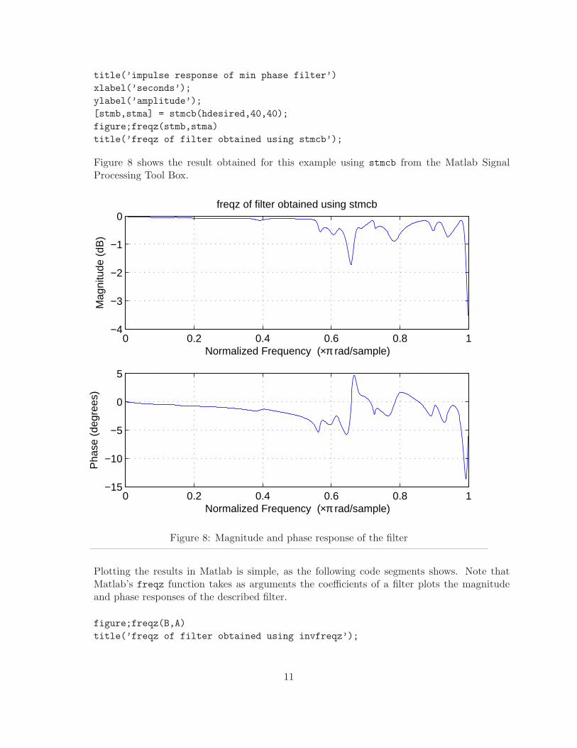
title(’impulse response of min phase filter’)
xlabel(’seconds’);
ylabel(’amplitude’);
[stmb,stma] = stmcb(hdesired,40,40);
figure;freqz(stmb,stma)
title(’freqz of filter obtained using stmcb’);
Figure 8 shows the result obtained for this example using stmcb from the Matlab SignalProcessing Tool Box.
0 0.2 0.4 0.6 0.8 1−15
−10
−5
0
5
Normalized Frequency (×π rad/sample)
Pha
se (
degr
ees)
0 0.2 0.4 0.6 0.8 1−4
−3
−2
−1
0
Normalized Frequency (×π rad/sample)
Mag
nitu
de (
dB)
freqz of filter obtained using stmcb
Figure 8: Magnitude and phase response of the filter
Plotting the results in Matlab is simple, as the following code segments shows. Note thatMatlab’s freqz function takes as arguments the coefficients of a filter plots the magnitudeand phase responses of the described filter.
figure;freqz(B,A)
title(’freqz of filter obtained using invfreqz’);
11
figure;freqz(stmb,stma)
title(’freqz of filter obtained using stmcb’);
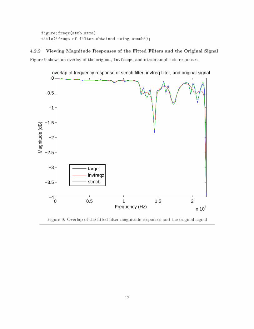
4.2.2 Viewing Magnitude Responses of the Fitted Filters and the Original Signal
Figure 9 shows an overlay of the original, invfreqz, and stmcb amplitude responses.
0 0.5 1 1.5 2
x 104
−4
−3.5
−3
−2.5
−2
−1.5
−1
−0.5
0
Frequency (Hz)
Mag
nitu
de (
dB)
overlap of frequency response of stmcb filter, invfreq filter, and original signal
targetinvfreqzstmcb
Figure 9: Overlap of the fitted filter magnitude responses and the original signal
12
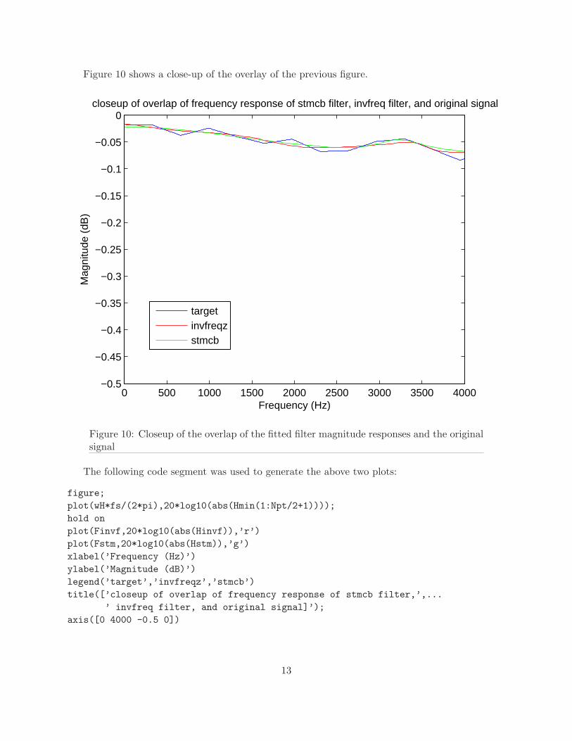
Figure 10 shows a close-up of the overlay of the previous figure.
0 500 1000 1500 2000 2500 3000 3500 4000−0.5
−0.45
−0.4
−0.35
−0.3
−0.25
−0.2
−0.15
−0.1
−0.05
0
Frequency (Hz)
Mag
nitu
de (
dB)
closeup of overlap of frequency response of stmcb filter, invfreq filter, and original signal
targetinvfreqzstmcb
Figure 10: Closeup of the overlap of the fitted filter magnitude responses and the originalsignal
The following code segment was used to generate the above two plots:
figure;
plot(wH*fs/(2*pi),20*log10(abs(Hmin(1:Npt/2+1))));
hold on
plot(Finvf,20*log10(abs(Hinvf)),’r’)
plot(Fstm,20*log10(abs(Hstm)),’g’)
xlabel(’Frequency (Hz)’)
ylabel(’Magnitude (dB)’)
legend(’target’,’invfreqz’,’stmcb’)
title([’closeup of overlap of frequency response of stmcb filter,’,...
’ invfreq filter, and original signal]’);
axis([0 4000 -0.5 0])
13
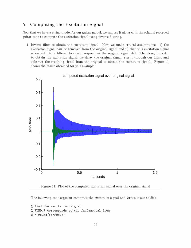
5 Computing the Excitation Signal
Now that we have a string-model for our guitar model, we can use it along with the original recordedguitar tone to compute the excitation signal using inverse-filtering.
1. Inverse filter to obtain the excitation signal. Here we make critical assumptions. 1) theexcitation signal can be removed from the original signal and 2) that this excitation signalwhen fed into a filtered loop will respond as the original signal did. Therefore, in orderto obtain the excitation signal, we delay the original signal, run it through our filter, andsubtract the resulting signal from the original to obtain the excitation signal. Figure 11shows the result obtained for this example.
0 0.5 1 1.5−0.3
−0.2
−0.1
0
0.1
0.2
0.3
0.4computed excitation signal over original signal
seconds
ampl
itude
Figure 11: Plot of the computed excitation signal over the original signal
The following code segment computes the excitation signal and writes it out to disk.
% find the excitation signal.
% FUND_F corresponds to the fundamental freq
N = round(fs/FUND);
14
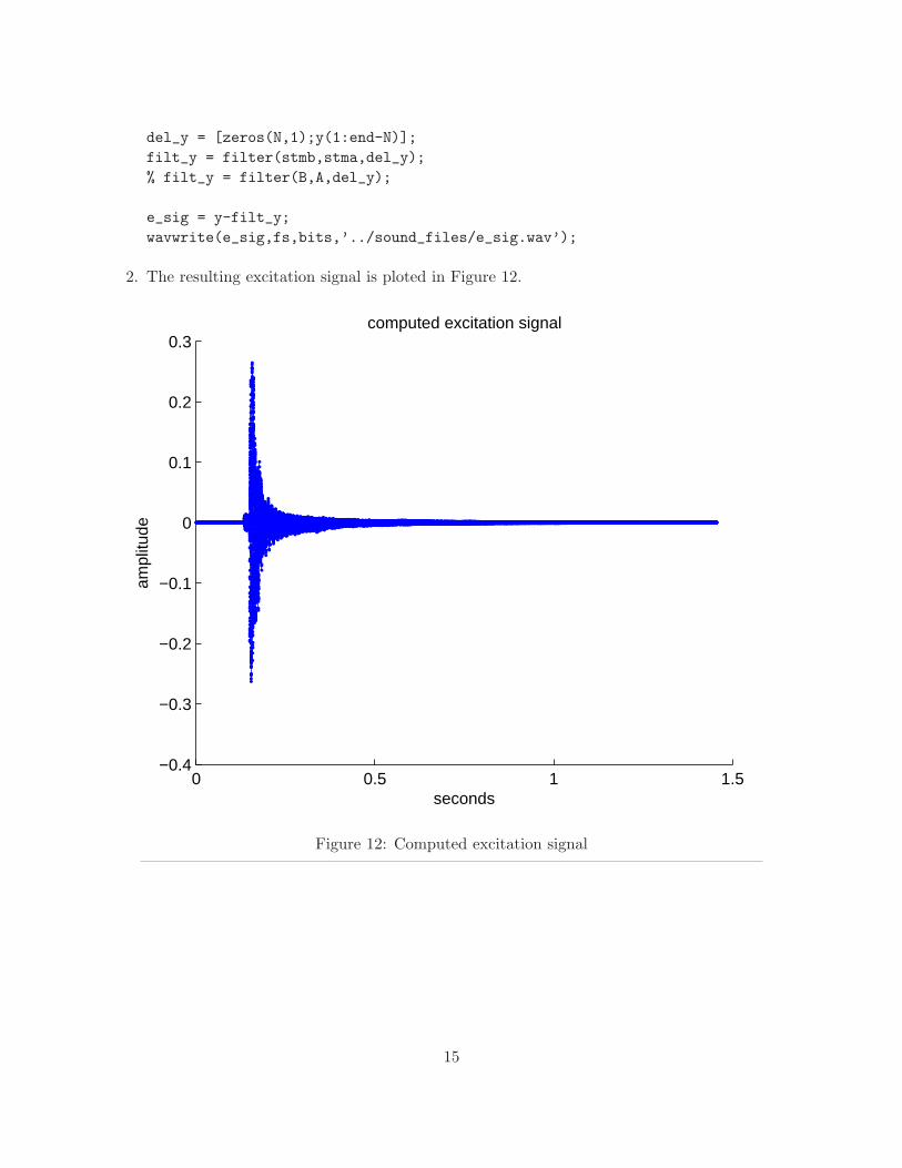
del_y = [zeros(N,1);y(1:end-N)];
filt_y = filter(stmb,stma,del_y);
% filt_y = filter(B,A,del_y);
e_sig = y-filt_y;
wavwrite(e_sig,fs,bits,’../sound_files/e_sig.wav’);
2. The resulting excitation signal is ploted in Figure 12.
0 0.5 1 1.5−0.4
−0.3
−0.2
−0.1
0
0.1
0.2
0.3computed excitation signal
seconds
ampl
itude
Figure 12: Computed excitation signal
15
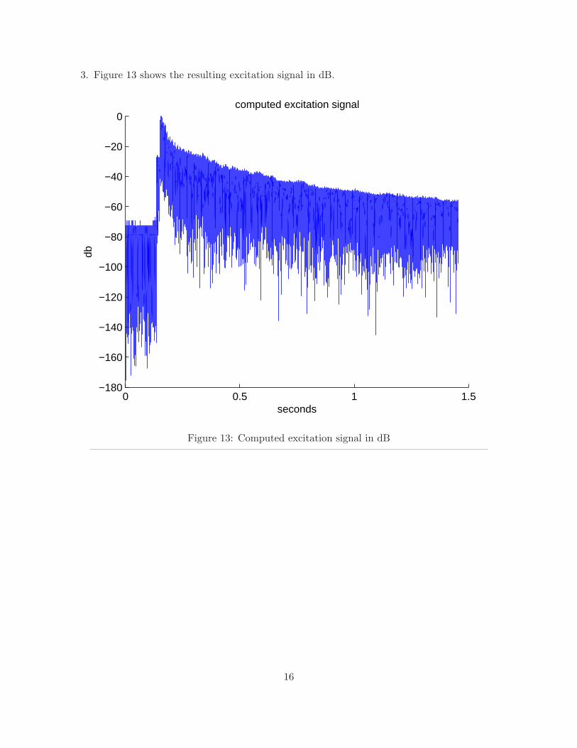
3. Figure 13 shows the resulting excitation signal in dB.
0 0.5 1 1.5−180
−160
−140
−120
−100
−80
−60
−40
−20
0computed excitation signal
seconds
db
Figure 13: Computed excitation signal in dB
16
6 Finding the Desired Gains of the Loop Filter for IndividualFrequencies
In 4, we had a graph of a filter with corresponding gains that we had estimated from the EDR. Inthis section, we go into detail as to how those gains were computed for filter-fitting from the EDR.
6.1 The Fundamental Frequency
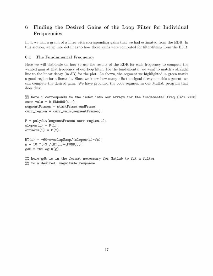
Here we will elaborate on how to use the results of the EDR for each frequency to compute thewanted gain at that frequency of our loop filter. For the fundamental, we want to match a straightline to the linear decay (in dB) for the plot. As shown, the segment we highlighted in green marksa good region for a linear fit. Since we know how many dBs the signal decays on this segment, wecan compute the desired gain. We have provided the code segment in our Matlab program thatdoes this:
%% here i corresponds to the index into our arrays for the fundamental freq (328.38Hz)
curr_vals = B_EDRdbN(i,:);
segmentFrames = startFrame:endFrame;
curr_region = curr_vals(segmentFrames);
P = polyfit(segmentFrames,curr_region,1);
slopes(i) = P(1);
offsets(i) = P(2);
RT(i) = -60*overlapSamp/(slopes(i)*fs);
g = 10.^(-3./(RT(i)*(FUND)));
gdb = 20*log10(g);
%% here gdb is in the format necessary for Matlab to fit a filter
%% to a desired magnitude response
17
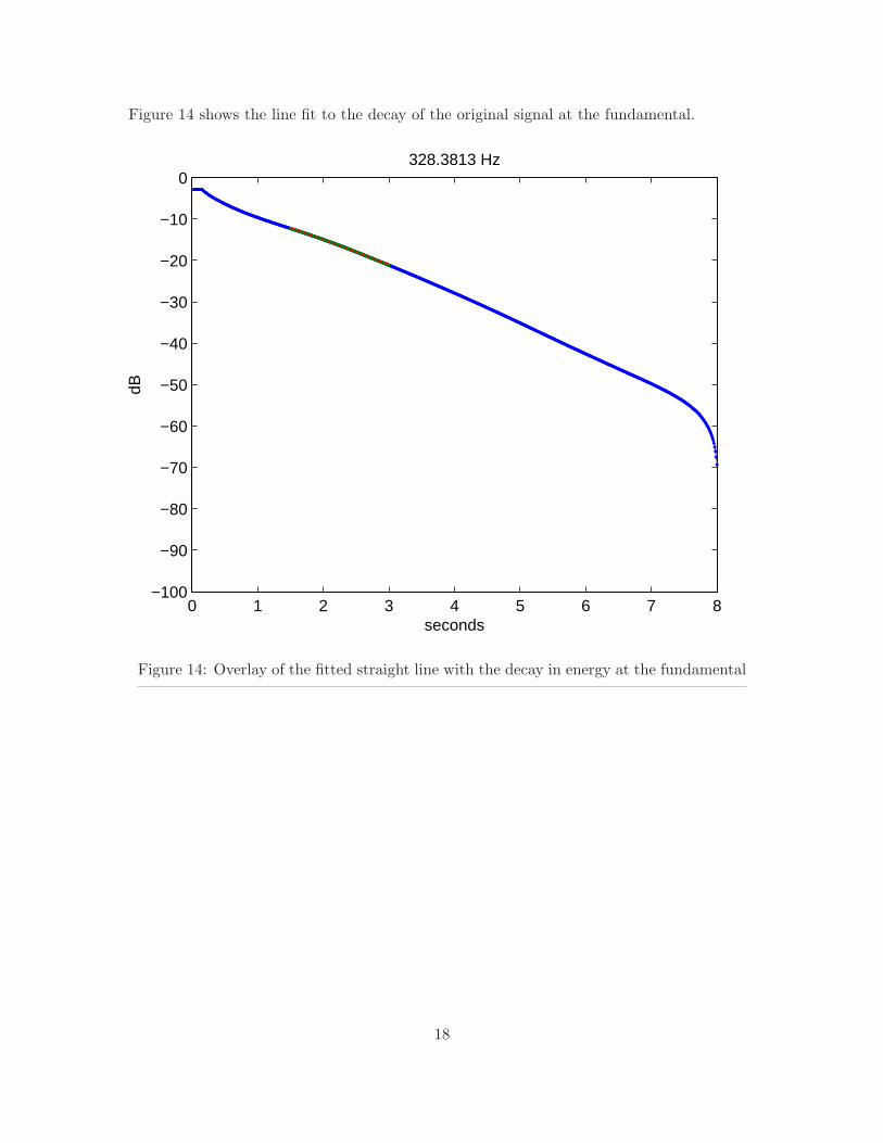
Figure 14 shows the line fit to the decay of the original signal at the fundamental.
0 1 2 3 4 5 6 7 8−100
−90
−80
−70
−60
−50
−40
−30
−20
−10
0328.3813 Hz
seconds
dB
Figure 14: Overlay of the fitted straight line with the decay in energy at the fundamental
18
Figure 15 shows the extrapolated delay beginning at 0dB to -100dB at the fundamental fre-quency.
0 5 10 15 20 25 30−60
−50
−40
−30
−20
−10
0328.3813 Hz: decay over time from fitted region
seconds
dB
Figure 15: Extrapolation of our fitted decay at the fundamental frequency
19
6.2 Other harmonics
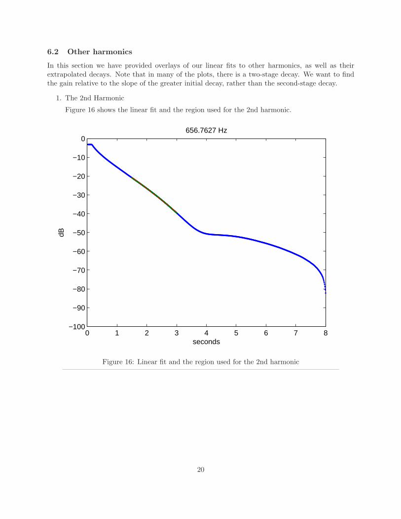
In this section we have provided overlays of our linear fits to other harmonics, as well as theirextrapolated decays. Note that in many of the plots, there is a two-stage decay. We want to findthe gain relative to the slope of the greater initial decay, rather than the second-stage decay.
1. The 2nd Harmonic
Figure 16 shows the linear fit and the region used for the 2nd harmonic.
0 1 2 3 4 5 6 7 8−100
−90
−80
−70
−60
−50
−40
−30
−20
−10
0656.7627 Hz
seconds
dB
Figure 16: Linear fit and the region used for the 2nd harmonic
20
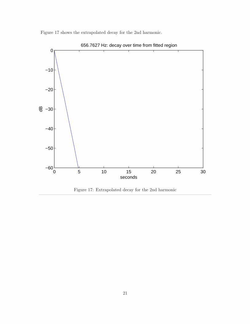
Figure 17 shows the extrapolated decay for the 2nd harmonic.
0 5 10 15 20 25 30−60
−50
−40
−30
−20
−10
0656.7627 Hz: decay over time from fitted region
seconds
dB
Figure 17: Extrapolated decay for the 2nd harmonic
21
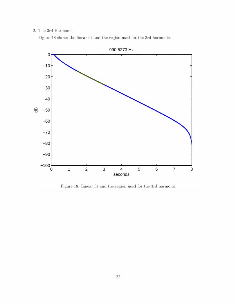
2. The 3rd Harmonic
Figure 18 shows the linear fit and the region used for the 3rd harmonic.
0 1 2 3 4 5 6 7 8−100
−90
−80
−70
−60
−50
−40
−30
−20
−10
0990.5273 Hz
seconds
dB
Figure 18: Linear fit and the region used for the 3rd harmonic
22
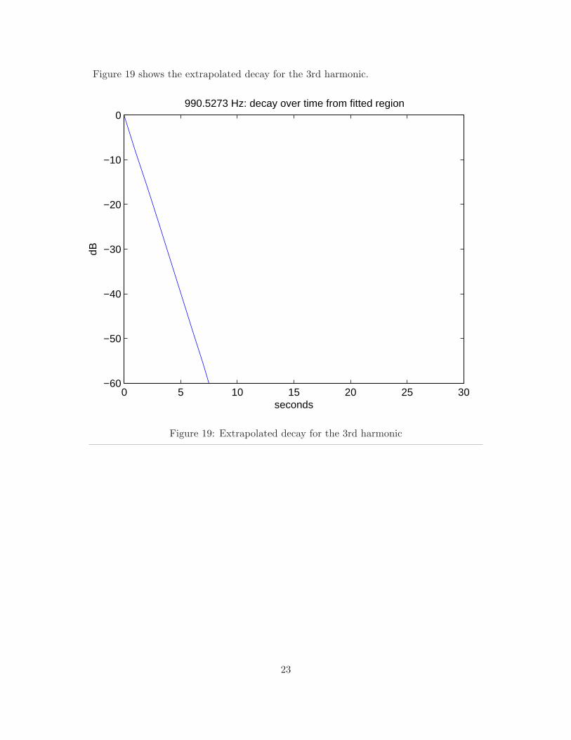
Figure 19 shows the extrapolated decay for the 3rd harmonic.
0 5 10 15 20 25 30−60
−50
−40
−30
−20
−10
0990.5273 Hz: decay over time from fitted region
seconds
dB
Figure 19: Extrapolated decay for the 3rd harmonic
23
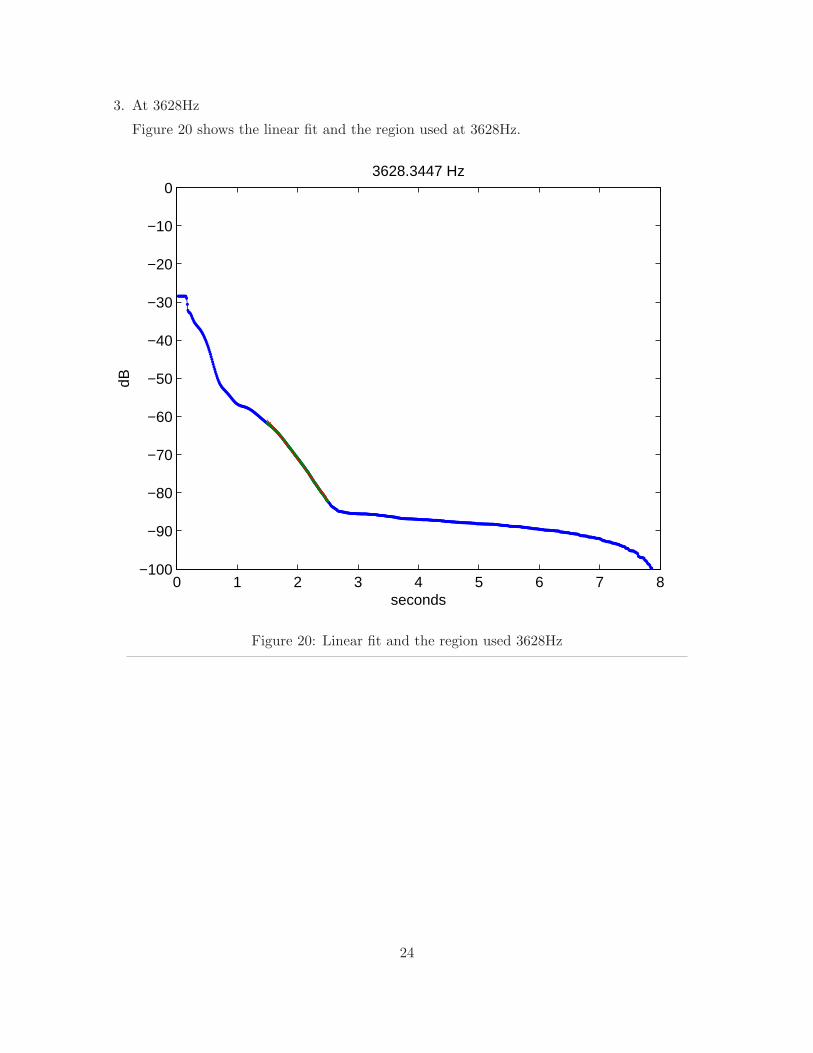
3. At 3628Hz
Figure 20 shows the linear fit and the region used at 3628Hz.
0 1 2 3 4 5 6 7 8−100
−90
−80
−70
−60
−50
−40
−30
−20
−10
03628.3447 Hz
seconds
dB
Figure 20: Linear fit and the region used 3628Hz
24
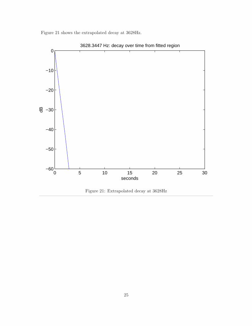
Figure 21 shows the extrapolated decay at 3628Hz.
0 5 10 15 20 25 30−60
−50
−40
−30
−20
−10
03628.3447 Hz: decay over time from fitted region
seconds
dB
Figure 21: Extrapolated decay at 3628Hz
25
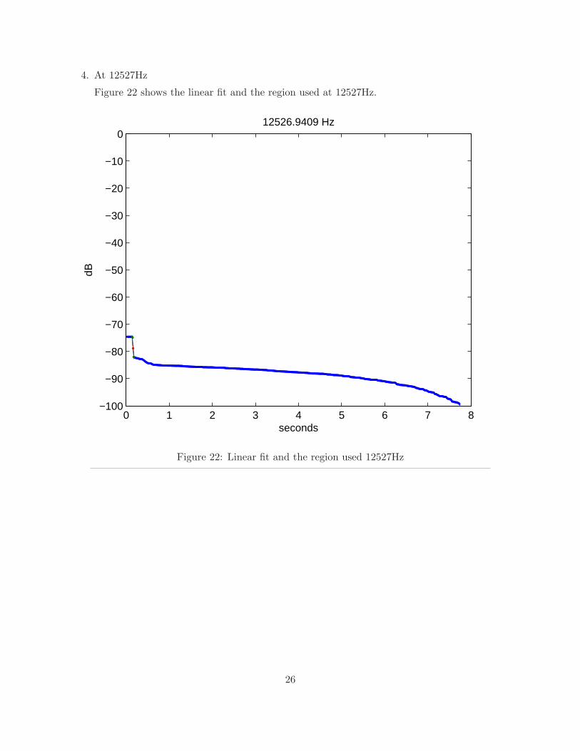
4. At 12527Hz
Figure 22 shows the linear fit and the region used at 12527Hz.
0 1 2 3 4 5 6 7 8−100
−90
−80
−70
−60
−50
−40
−30
−20
−10
012526.9409 Hz
seconds
dB
Figure 22: Linear fit and the region used 12527Hz
26
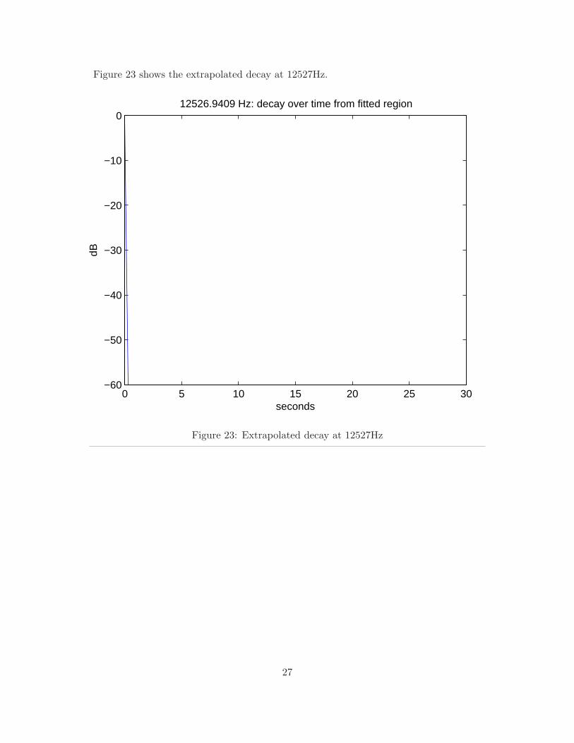
Figure 23 shows the extrapolated decay at 12527Hz.
0 5 10 15 20 25 30−60
−50
−40
−30
−20
−10
012526.9409 Hz: decay over time from fitted region
seconds
dB
Figure 23: Extrapolated decay at 12527Hz
27
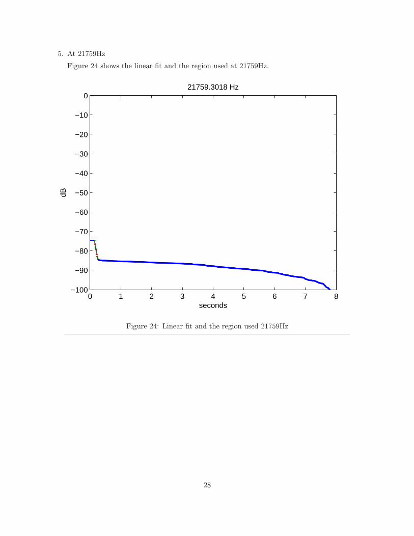
5. At 21759Hz
Figure 24 shows the linear fit and the region used at 21759Hz.
0 1 2 3 4 5 6 7 8−100
−90
−80
−70
−60
−50
−40
−30
−20
−10
021759.3018 Hz
seconds
dB
Figure 24: Linear fit and the region used 21759Hz
28
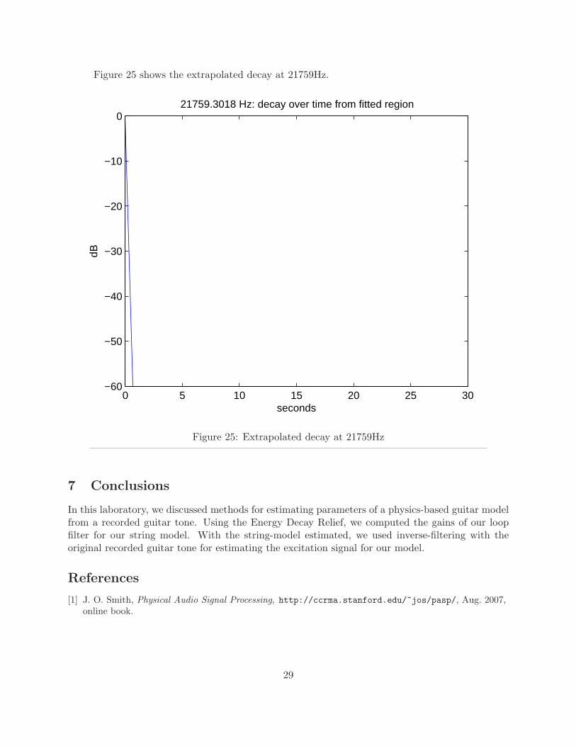
Figure 25 shows the extrapolated decay at 21759Hz.
0 5 10 15 20 25 30−60
−50
−40
−30
−20
−10
021759.3018 Hz: decay over time from fitted region
seconds
dB
Figure 25: Extrapolated decay at 21759Hz
7 Conclusions
In this laboratory, we discussed methods for estimating parameters of a physics-based guitar modelfrom a recorded guitar tone. Using the Energy Decay Relief, we computed the gains of our loopfilter for our string model. With the string-model estimated, we used inverse-filtering with theoriginal recorded guitar tone for estimating the excitation signal for our model.
References
[1] J. O. Smith, Physical Audio Signal Processing, http://ccrma.stanford.edu/~jos/pasp/, Aug. 2007,online book.
29