Reallocation and Technology:

Evidence from the U.S. Steel Industry ∗

Allan Collard-Wexler and Jan De LoeckerNYU and NBER, and Princeton University, NBER and CEPR

First version February 2012, current version January 2013

Abstract

We measure the impact of a drastic new technology for producing steel – theminimill – on the aggregate productivity of U.S. steel producers, using uniqueplant-level data between 1963 and 2002. We find that the sharp increase in theindustry’s productivity is linked to this new technology, and operates throughtwo distinct mechanisms. First, minimills displaced the older technology, calledvertically integrated production, and this reallocation of output was responsiblefor a third of the increase in the industry’s productivity. Second, increasedcompetition, due to the expansion of minimills, drove a substantial reallocationprocess within the group of vertically integrated producers, driving a resurgencein their productivity, and consequently of the industry’s productivity as a whole.

1 Introduction

Identifying the sources of productivity growth of firms, industries, and countries, has

been a central question for economic research. There remain, however, many em-

pirical obstacles to credibly identify the underlying sources of productivity growth.

First, the measurement of productivity at the producer level typically requires an

∗This project was funded by the Center for Economic Policy Studies (CEPS) at PrincetonUniversity and the Center for Global Economy and Business (CGEB) at New York University. Wewould like to thank Jun Wen for excellent research assistance, and Jonathan Fisher for conversationsand help with Census Data. We would like to thank Rob Clark, Liran Einav, Ariel Pakes, KathrynShaw, Chad Syverson, Raluca Dragusanu, and seminar participants at many institutions. Thispaper uses restricted data that was analyzed at the U.S. Census Bureau Research Data Center inNew York City. Any opinions and conclusions expressed herein are those of the authors and donot necessarily represent the views of the U.S. Census Bureau. All results have been reviewed toensure that no confidential information is disclosed.

1

estimate of the production function and, therefore, has to confront both the endo-

geneity of inputs and unobserved prices for inputs and outputs. Second, it is difficult

to observe potential explanatory variables at the producer level, such as technology,

competition, and management practices.1 Finally, in order to establish causality,

exogenous shifters of such variables are required in order to trace out their effects

on productivity.

In this paper, we shed light on the role of a specific driver: the arrival of a new

technology. We evaluate the impact of a drastic technological change on aggregate

productivity growth, while at the same time controlling for potentially additional

drivers of productivity growth such as international competition, geography, and

firm-level factors such as organization and management.

A recent literature has emphasized the distinction between the productivity ef-

fects that occur at the producer level, and those realized by moving resources be-

tween producers – i.e., the reallocation mechanism. Although it is well established,

by now, at both a theoretical and empirical level that the reallocation of resources

across producers is important in explaining aggregate outcomes, it has been very

hard to identify the exact mechanisms behind it.2 In this paper, we focus on the

role of technology and associated changes in competition in driving reallocation.

We examine one particular industry, the U.S. steel sector, for which we have

detailed producer-level production and price data. Our setting is well suited to

measuring the role of technological change, since we directly observe the exogenous

arrival of a new production process – the minimill – at the plant level. In addition,

we observe detailed output and input data, including physical measures of inputs

and outputs, as well as standard revenue and expenditure data, to obtain measures

of productivity and market power. These inputs and outputs are remarkably un-

changing over a forty year period, and the steel products shipped in the sixties are

1See Syverson (2011) for an excellent overview of the various potential determinants of pro-ductivity at both the producer and industry level. Two prominent studies on the triggers ofproductivity growth are Schmitz (2005) and Olley and Pakes (1996), who study the role of twosuch triggers: import competition in the iron ore market and deregulation in the telecommuni-cations market. Hortacsu and Syverson (2004), Bloom, Eifert, Mahajan, McKenzie, and Roberts(2011), and Jarmin, Klimek, and Miranda (2009) show that factors such as vertical integration,management, and large retail chains lead to systematic differences in productivity between plantsand consequently, have implications for aggregate industry performance.

2For instance Melitz (2003), shows how trade liberalization impacts aggregate productivitythrough a reallocation towards more-productive firms, while Foster, Haltiwanger, and Krizan (2001)and Bartelsman, Haltiwanger, and Scarpetta (2009) document the role of reallocation empirically,using firm-level data.

2

very similar to those shipped in 2000. Thus, productivity growth in steel is almost

uniquely driven by process innovation, rather than through the introduction of new

goods. The long panel, 1963-2002, of steel producers allows us to study the long-run

implications of increased competition, such as the (slow) entry and exit process.

The U.S. steel industry shed about 75 percent of its workforce between 1962

to 2005, or about 400,000 employees. This dramatic fall in employment has far-

reaching economic and social implications. For example, between 1950 to 2000,

Pittsburg – which used to be the center of the U.S. Steel Industry – dropped from

the 10th largest city in the United States to the 52nd largest.

While employment in the Steel Sector fell by a factor of five, shipments of steel

products in 2005 reached the same level of the early sixties.Thus output per worker

has grown by a factor of five, while total factor productivity (TFP) increased by

38 percent. Over the last three decades, this makes the steel sector one the fastest

growing industries among large manufacturing industries, behind only the computer

software and equipment industries. We highlight the special features of the U.S. steel

industry in Table 1, where we report the change in output, employment and TFP

over the period 1972-2002 for the U.S. steel sector and compare it to the mean and

median manufacturing sector’s experience.

Table 1 points out the unique feature of the steel industry: The period of impres-

sive productivity growth, 28 percent compared to the median of 3 percent, occurred

while the sector contracted by 35 percent. The starkest difference is the drop in

employment of 80 percent compared to a decline of 5 percent for the average sector.

We find that the main reason for the rapid productivity growth and the asso-

ciated decline in employment is neither a steady drop in steel consumption, nor a

consequence of globalization. Nor is it a displacement of production away from the

midwest. The increase in productivity can be directly linked to the introduction of

a new production technology, the steel minimill. The minimill displaced the older

technology, called vertically integrated production, and this reallocation of output

was responsible for about a third of the increase in the industry’s total factor pro-

ductivity. In addition, minimills’ productivity steadily increased through a slow

process of learning by doing. We directly attribute almost half of the aggregate

productivity growth to the entry of this new technology.

However, the older technology was not entirely displaced. Instead, vertically

integrated producers experienced a dramatic resurgence of productivity and, by

2002, are on average as productive as minimills. This resurgence was not driven

3

by improvements at integrated plants. Instead, less-productive vertically integrated

plants were driven out of the industry, and output was reallocated to more-efficient

producers. We find that the increased competition, due to the entry and expansion of

minimills, was directly responsible for this reallocation process among incumbents.

In addition to identifying the exact mechanisms underlying productivity growth,

which are of interest to a growing literature on reallocation and productivity dis-

persion, the steel industry is also important in and of itself. Even today, it is one

of the largest sectors in U.S. manufacturing: In 2007, steel plants had shipments of

over 100 billion dollars, of which half was value added. Therefore, understanding

the sources of productivity growth in this industry is of independent interest.

The remainder of the paper is organized as follows. In Section 2, we discuss

the rich plant-level data from the Census. In Section 3, we present five key facts

that help guide the empirical analysis, which we take up in Section 4. We discuss

alternative explanations in Section 5 and conclude in Section 6.

2 Data

We study the production of steel: plants engaged in the production of either carbon

or alloy steels.We rely on detailed Census micro data to investigate the mechanisms

underlying the impressive productivity growth in the U.S. steel sector. Our analysis

is based on plant-level production data of U.S. steel mills from 1963 to 2002.

We use data provided by the Center for Economics Studies at the United States

Census Bureau. Our primary sources are the Census of Manufacturers (CMF), the

Annual Survey of Manufacturers (ASM), and the Longitudinal Business Database

(LBD). We select plants engaged in the production of steel, coded in either NAICS

(North American Industrial Classification) code 33111, or SIC (Standard Industrial

Classification) code 3312. The CMF is sent to all steel mills every five years, while

the ASM is sent to about 50 percent of plants in non-Census years. However, the

ASM samples all plants with over 250 employees and, encompasses over 90% of the

output of the steel sector.

In addition, we collect data on the products produced at each plant using the

product trailer to the CMF and the ASM, and, collect the materials consumed by

these plants from the material trailer to the CMF.

We rely on our detailed micro data to break up steel mills into two technologies:

Minimills (MM, hereafter) and Vertical Integrated (VI, hereafter) Producers. VI

4

production takes place in two steps. The first stage takes place in a blast furnace,

which combines coke, iron ore, and limestone to produce pig iron and slag. The pig

iron, along with oxygen and fuel, is then used in a basic oxygen furnace (BOF) to

produce steel.3 The steel products produced in either MM or VI plants are shaped

into sheets, bars, wire, and tube in rolling mills. These rolling mills are frequently

collocated with steel mills, but can also be freestanding units.

In contrast, MMs are identified primarily by the use of an electric arc furnace

(EAF) to melt down a combination of scrap steel and direct reduced iron. Because

these mills have a far smaller efficient scale, they are, on average, an order of mag-

nitude smaller than vertically integrated producers. Historically EAFs were used to

produce lower-quality steels, such as those used to make steel bars, while virtually

all steel sheet (needing higher-quality steel), was produced in BOFs. However, since

the mid-1980s, innovation in the EAFs has enabled them to produce certain types

of steel sheet products, as well.4

We classify plants into minimills, vertically integrated plants, and rolling mills

using their response to a specific questionnaire on steel mills attached to the 1997,

2002, and 2007 CMF. For prior years, we use the material and products produced by

each plant to identify MM and VI plants. More detail on the classification of plants

can be found in the Data Appendix. Table A.3 shows summary statistics for the

sample of MM and VI plants. The average VI plant had shipments of 647 million

dollars, of which 47 percent is value added, while the average MM plant shipped

153 million dollars, of which 44 percent is value added.

3 Key Facts in the U.S. steel sector 1963-2002

In this section, we briefly go over some key facts of the U.S. steel sector. These

facts will be important to keep in mind when we analyze the sources of productivity

growth.

3There were a few open-hearth furnaces in operation during the sample period. However, as ofthe late 1960s, open-hearth plants account for only a very small portion of output, and the lastopen-hearth plant closed in 1991. See Oster (1982) for more on the diffusion of BOF mills.

4EAFs have a long history in steel making. However, before the 1960s, they primarily producedspecialty steels.

5

3.1 Stagnant Shipments, Rising Productivity

From Table 1, we know that the productivity growth in the U.S. steel sector was

one of the fastest in manufacturing. To better understand this period of impressive

productivity growth, we plot total output next to labor and capital use in Figure

1. An important observation is that the period of productivity growth came about

while the industry as a whole contracted severely: Steel producers sold about 60

billion dollars in 1960 and, reached 100 billion dollars in shipments by the early

seventies. A decade later, only 40 billion dollars were shipped, or, put differently,

the sector’s shipments decreased by more than half.

Total employment, on the other hand, consistently decreased, even during the

recovery of output in the late eighties and throughout the nineties. The employment

panel of Figure 1 shows that total employment fell from 500,000 to 100,000 employ-

ees. This is one of the sharpest drops in employment experienced by any sector in

the U.S. economy. By 2000, the steel industry employed a fifth of the number of

workers that it did in 1960, while production of steel went from 130 million tons

in 1960 to 110 million tons in 2000. This implies that output per worker increased

from 260 to 1100 tons.5 Total material use tracks output quite closely, while labor

and capital fell continuously over the entire period, which suggests that TFP had

to increase to offset the sharp drop in labor and capital.6

3.2 A New Production Technology: Minimills

The entry of minimills in steel production constituted a drastic change in the actual

production process of steel products. A natural question to ask is whether MM

are any different than the traditional VI steel producers. We rely on a descriptive

OLS regression where we regress direct measurable characteristics on an indicator

variable, whether a plant is a vertically integrated producer. We consider a log

specification such that the coefficient on the technology dummy directly measures

the percentage premium of VI plants.

Table A.2 lists the set of estimated coefficients, and confirms that vertically

integrated producers are, on average, four times bigger, as measured by the large

coefficients on shipments, value added, and inputs. For example, VI plants, on

5Shipments of steel in tons are collected from various Iron and Steel Institute Annual StatisticalReports (American Iron and Steel Institute, 2010).

6For this aggregate analysis, we rely on the NBER’s five-factor TFP estimate. See Bartelsman,Becker, and Gray (2000) for more detail.

6

average, ship 144 percent more than MM. Moreover, VI producers generate about 20

percent more shipments per worker, which suggests that they are more productive.

However, when we combine the coefficients on all three inputs (labor, materials and

capital) with the shipment premium, we see that total factor productivity (TFP)

of MM is at least as high as that of VI producers. We turn to a more precise

comparison of TFP across technologies in Section 4.

In addition to the average premium over the entire sample, we report time-

specific coefficients. Across all the various characteristics, the VI coefficient falls

over time. Most notably, shipments per worker were 23-percent higher for VI plants

in 1963, but by 2002, there was no significant difference between the two technologies

in terms of labor productivity. This pattern suggests that, over time, VI and MM

producers became more alike, although VI producers still produce on a larger scale.

The coefficients on wages of six percent, shown in the last row of Table A.2,

confirms the well-known fact that VI producers, on average, pay higher wages. This

is likely due to the impact of unionization – minimill workers typically being non-

unionized.7 It is interesting to note that the wage gap between the technologies

closes over time.

An important difference between MM and VI producers is the set of products

they manufacture. Figure 2 shows that in 1997 MMs accounted for 59 percent

and 68 percent of shipments of steel ingots and hot-rolled bar, but only 15 percent

and 14 percent of hot and cold rolled sheet. MM typically produce lower quality

steel products, which are generally thicker products, while VI plants produce higher

quality products, which are usually sheet products. However, the product mix

accounted for by MM changed dramatically over the last 40 years. Figure 2 shows

that, in 1977, MMs produced 27 percent of steel ingots and 24 percent of hot-rolled

bar. Between 1977 and 1982, MMs increased their share of these products to 40

percent, and by 2002, 81 percent of hot-rolled bar was produced by MMs. As stated

above, in 1997, only 15 percent and 14 percent of hot and cold rolled sheet are

produced by MMs.8 Thus, the market share of MM in the higher-quality product

segments, sheet products, was rather stable up to 1997, after which their market

shares did increase substantially.

7See Hoerr (1988) – and in particular, page 16 – for evidence of the role of unionization on wagesfor VI and MM producers.

8Giarratani, Gruver, and Jackson (2007) discuss the entry of Minimills into the production ofsheet products around 1990.

7

3.3 A Stable Product Mix over Time

We list the product mix of the steel industry in Table A.3. We break down steel

into various products: a) hot-rolled steel sheet (HRS) b) hot-rolled bar (HRB) c)

cold-rolled sheet (CRS) d) ingots and shapes e) pipe and tube (P&T) f) Wire g)

cold-finished bars (CFB), and h) coke oven and blast furnace products (Blast). Over

40 years, the product mix for steel has barely changed. Hot-rolled sheet account for

23 percent of shipments in 1963 and 31 percent in 2002, and hot-rolled bar account

for 23 percent of shipments in 1963 and 22 percent in 2002.

The fact that the steel industry’s products have been unchanged is essential for

our identification of productivity growth, as the industry’s production process has

changed far more than its products.

3.4 Heterogeneous Price Trends Across Products

While the product mix of steel producers has been relatively unchanged from 1963 to

today, the prices for these products have dropped considerably, which is unsurprising

given the large increases in TFP in the industry. Figure 6 presents the price indices

for the four main products – hot and cold rolled sheet, hot rolled bar and steel ingots

– which, taken together, represent 80 percent of shipments in 1997.9

Figure 6 shows that the prices of all steel products followed a very similar, and

gradually increasing, pattern up to 1980. But from 1982 to 2000, there is a 50-

percent drop in the real price of steel. This implies that, while shipments of steel in

dollars dropped since 1980, the quantity shipped has gradually increased since the

mid-eighties (see Panel 1 of Figure 1).10

In addition, when we decompose these price trends further, we find that the

prices of hot-rolled bars and steel ingots have fallen faster than the prices for hot

and cold rolled sheet. While sheet steel is produced primarily by VI producers, prices

for bar and ingot products fell by ten percent more than those for sheet products

in 1982-1984. This occurred precisely at the point at which MM saw an increase of

their market share of bar and ingot products.

In order to correctly identify the productivity effect of the arrival of the minimills,

9We have taken care to deflate these price indices by the GDP deflator to show price trends forsteel relative to the rest of the economy.

10Annual reports of the American Iron and Steel Institute (2010), where total tons of steel arerecorded annually, indicate that quantity produced increased by about thirty percent between 1982and 2002.

8

and their associated increased competition, it will therefore be imperative to control

for price differences across plants and time.

3.5 Simultaneous Entry and Exit

From Figure 1, we know that the number of plants increased over time. In Table 2,

we go a step further, and show both the number of MM and VI plants that entered

or exited, and as well as the market share these plants represent. There was marked

entry of new plants in the early eighties, a period during which the industry as a

whole was severely contracted.

The market share of plants entering from 1982 to 1992 was 20 percent, versus

five percent in the previous two decades, while the market share of exitors was 18

percent during this period. Most entry in this period was due to minimills, and

most exit was from vertically integrated producers.11 From these entry and exit

statistics, we expect an important role for entry and exit in explaining productivity

growth.

4 Drivers of productivity growth

The previous section highlighted the difference in performance between MM and

VI producers, and suggests a large potential role for reallocation across these tech-

nologies in explaining productivity growth. This paper is concerned with studying

the productivity differences in detail and verify the extent to which the entry of

minimills contributed to the stark aggregate productivity growth in the industry,

and we proceed in two steps.

First, we start by presenting our empirical framework. Second, we rely on our

productivity estimates to verify the importance of reallocation, both across and

within technology, in productivity growth. We consider both static and dynamic

decompositions, which enables us to investigate the importance of entry and exit in

productivity growth. Finally, we relate a direct measure of competition – markups

– to the reallocation analysis by connecting markups to the analysis of reallocation,

which relates market shares to productivity.

11This phenomenon, the speeding up of exit and entry during a downturn, has been documentedby Bresnahan and Raff (1991) in the motor vehicles industry during the Great Depression.

9

4.1 Productivity Differences Across Technology

Denote each technology – either MM or VI – as ψ ∈ V I,MM.12 A plant i at

time t can produce output Qijt of a given product j, using a technology ψ specific

production technology:

Qijt = Fψ,t(Lijt,Mijt,Kijt) exp(ωit). (1)

Our notation highlights that VI and MM producers rely on different technologies,

which we allow to vary over time. As is common in the literature, productivity ωit is

modeled as a Hicks-neutral term. Moreover, we assume that productivity is plant-

specific.

4.1.1 Measurement

Recovering productivity using revenue and expenditure data requires that we correct

for potential price variation across plants and time, for both output and inputs.

Below, we describe our procedure briefly, and Appendix C provides more details.

In order to guarantee that we recover productivity, ωit, using plant/product

revenue data, we construct a plant-specific price (Pit) . We assume that each product

j is homogeneous, and we directly observe each price Pjt in the product-level BLS

price data. Furthermore, we follow the literature and consider a Cobb-Douglas

specification by type. We can, therefore, write equation (1) as:

Rijt = LαlijtMαmijt K

αkijt exp(ωit)Pjt. (2)

Since we are interested in recovering a measure of productivity at the plant level, we

aggregate product-level sales up to plant-level sales. A common restriction in these

type of data is that we do not directly observe the input use by product (see Foster,

Haltiwanger and Syverson 2008). We allocate inputs across products using product-

specific sales shares, sijt =RijtRit

, such that Xijt ≡ sijtXit with X = L,M,K.13

12Plants cannot change from one technology to another. In the steel industry, a plant neverswitches technology, such as becoming a minimill. This is in contrast to the a setting of technologyadoption. See Van Biesebroeck (2003) for an empirical analysis of technology adoption in US carmanufacturing.

13As discussed in detail in Appendix C, this implies that we implicitly restrict markups to becommon across products within a plant. We are not interested in explaining within-plant markupdifferences across products, but mainly aim to recover measures of plant-level productivity that arenot contaminated by price variation across plants and time.

10

After aggregating (2) to the plant level we obtain:

Rit∑j sijtPjt

= LαlitMαmit Kαk

it exp(ωit). (3)

Although the focus in the literature has mostly been on the heterogeneity of

output prices, input price variation potentially plagues the measurement of pro-

ductivity as well. The data on intermediate input use, Mit, are potentially the

most contaminated by input price variation, both in the the time series, and in the

cross-section, particularly between MM and VI plants. The two technologies use

vastly different intermediate inputs, or use inputs at very different intensities and,

therefore, we expect the relevant input price to vary substantially across plants of

different technologies.

We construct our input price deflators in a similar way as the output price

deflator. First, we need to distinguish between our three main input categories:

labor, intermediate inputs and capital. We directly observe labor Lit: hours worked

at the plant-level. For capital, we rely on the NBER capital deflator (P kt ) to correct

the capital stock series.

We construct an intermediate input price index Pnt for each intermediate input

n, where n = Fuels, Electricity, Coal for Coke, Iron Ore, and Scrap Steel, using

either the NBER fuel price deflator, or reported quantities and costs in the material

trailer to the CMF (which allow us to back out prices). We construct a plant-specific

input price index (PMit ) using a weighted average of these intermediate input specific

prices, Pnt, where the shares are the share of an intermediate n in total intermediate

input use. Deflated intermediate input use is, thus, given by Mit =∑

nMEint

PMit, where

MEint is the expenditure of plant i, at time t, on intermediate input n.

We present the time series pattern of our constructed input price index in Figure

B.1. We compare the publicly available NBER Material Price Index (NBER MPI)

with our constructed input price index. We compute the mean of the latter by

technology and find that the NBER MPI follows our price index closely. However,

the aggregate input price index hides the heterogeneity in input prices, in particular

during the energy price spike in the late seventies and early eighties. This is par-

ticularly important given our focus on correctly identifying productivity differences

across technology: We would overestimate the productivity premium for minimills.

While input prices were very similar around 1972, by 1982, integrated producers

faced almost 20-percent-higher input prices and this fact would artificially increase

11

the productivity premium for minimills.

We estimate the production function using our constructed output and input

price deflators using:

qit = βllit + βmmit + βkkit + ωit + εit, (4)

where lower cases indicate logs of deflated variables when appropriate.14 We allow

for unanticipated shocks to production and measurement error in output and prices,

as captured by εit.15 In the next section, we report the production function coeffi-

cients, and the corresponding minimill productivity premium, if any, under various

specifications.

4.1.2 Production function coefficients and technology premium

We start by considering a few baseline specifications for the standard Cobb-Douglas

production function. Table 3 presents estimates of the production function. Columns

I, II and III show results with output defined as sales deflated by an aggregate price

deflator, while Columns IV through IX show estimates using plant-level output and

input deflators. Columns III, VI and IX present estimates using an investment con-

trol function approach as discussed in Ackerberg, Benkard, Berry, and Pakes (2007).

We underscore that it is important in this context to explicitly allow the underlying

demand and technology factors to vary with the technology type. More specifically,

we index the investment policy function, the exit rule and the productivity process

with the technology type indicator. Appendix C.1 provides more details on the es-

timation procedure. We compare our results to a few baseline OLS estimates, listed

in the other columns, to highlight the importance of our corrections.

The production function coefficients, across all specifications, are stable and have

reasonable estimates of returns to scale and output elasticities. An important test

for our purpose is to check whether minimills and vertically integrated producers

rely on different input factor shares. In order to test this, we simply interact every

coefficient with our technology type dummy and run a F -test on the joint significance

of the interacted coefficients. In doing so, we cannot reject that both technologies

14E.g., qit = ln(

Rit∑j sijtPjt

)and mit = ln

(∑n

MEintPnt

).

15Formally the inclusion of εit is compatible with the existence of measurement error and unan-ticipated shocks in both revenue and price data. E.g. we observe revenue in the data and it relatesto a firm’s measure as follows: Rit = R∗it exp(εit). The error term εit thus captures, potentially,multiple iid error terms. The distinction is not important for our analysis.

12

produce under the same output elasticities of labor, materials, and capital. At first,

it might seem surprising that, for instance, the coefficient on materials does not

vary across technologies. However, note that this coefficient reflects the importance

of the total use of intermediate inputs in final production. Aggregating over the

various intermediate inputs into Mit masks the distinct inputs used in production,

which differ tremendously by technology.16

Four main results emerge from this analysis. First, minimills are, on average,

more productive, as indicated by a negative coefficient on the VI dummy. Under

specification I, minimills have a three-percent-higher TFP than vertically integrated

producers, but this is not statistically significant. This result is surprising, both

since industry participants believe that minimills are more productive, and since

these plants show large increases in market share over the sample period.

Second, the TFP premium for minimills decreases over time as indicated by the

positive coefficient of 0.3 percent on the technology-year. Although this coefficient

is relatively small in magnitude, one has to keep in mind that our sample covers 40

years, which implies that by the end of our sample, the TFP premium for MM has

disappeared. This will be important when we compute our decompositions – i.e., we

expect the impact of minimills in aggregate productivity growth to be concentrated

at the beginning of the sample.

Third, the results in Panel B demonstrate the importance of controlling for unob-

served prices in the revenue-generating production function (Panel A) and confirm

the findings of De Loecker (2011). In particular when we correct for plant-specific

prices, we find that the minimill TFP premium is twice as high, and becomes sig-

nificant. The impact of including detailed price data on the technology coefficient

is as expected since we know from Figure 6 that VI plants are active in the rela-

tively higher-quality segments, where producer prices are higher. Therefore, when

we do not properly deflate the sales data, the productivity premium for minimills is

dampened. The results in column IX indicate that correcting for differences in in-

put prices across plants and time, in particular across technology, has the predicted

effect: The magnitude of the minimill productivity premium is somewhat lower, 6.3

percent versus 11 percent, but it is still highly significant and substantial. The lower

point estimate reflects the pattern of input prices in Figure B.1, that input prices

16For instance, in 2002, Iron and Steel Scrap represented 42 percent of the coded material inputsfor minimills, and Coal for the production of Coke represented 15 percent of the coded materialinputs for vertically integrated plants.

13

for VI producers were higher in the late seventies and early eighties.

The impact of our price corrections are as expected. To illustrate our results,

we find it useful to write out the potential bias induced by not deflating either

output or inputs in light of our productivity analysis. We refer the reader to De

Loecker (2011) and De Loecker, Goldberg, Khandelwal, and Pavcnik (2012) for more

details on the impact of unobserved output and input prices, respectively. Using

our production function, it is easy to show that, without deflating, the following

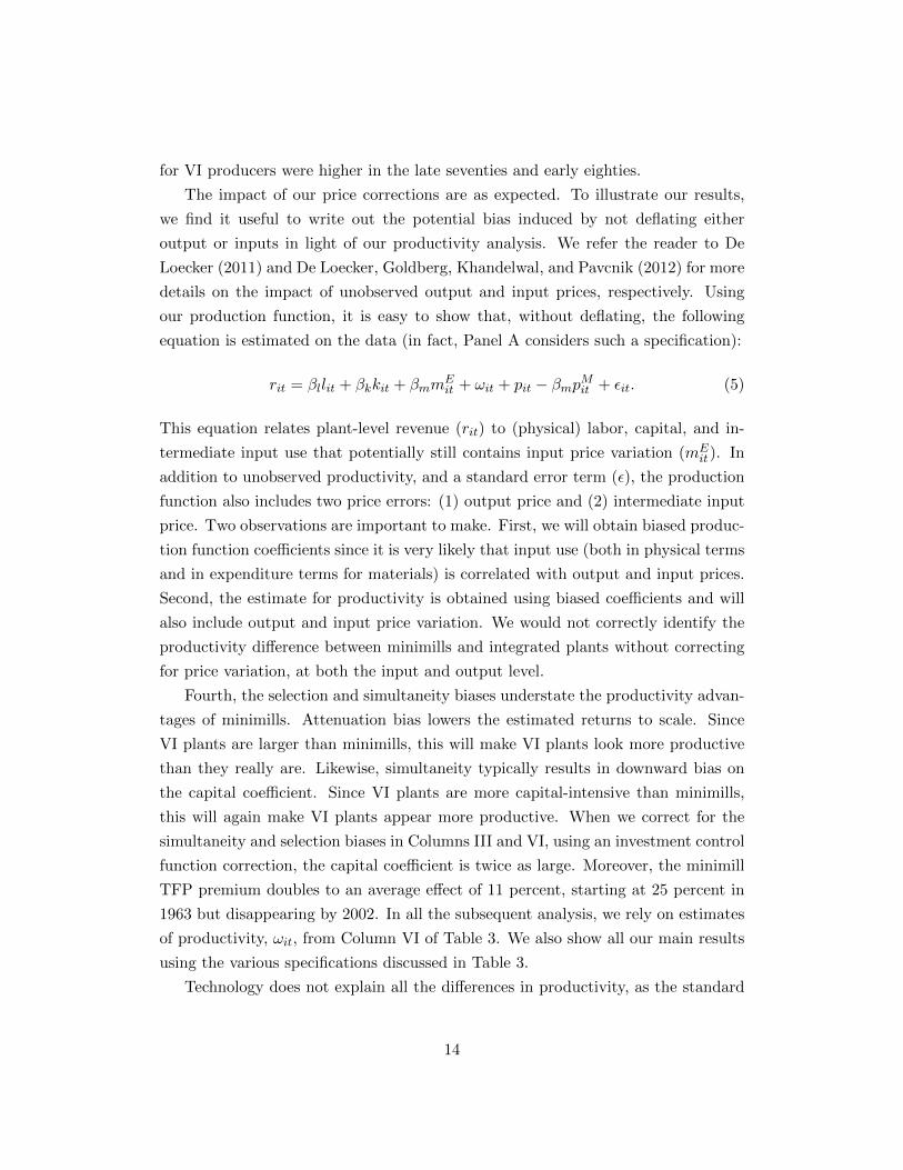
equation is estimated on the data (in fact, Panel A considers such a specification):

rit = βllit + βkkit + βmmEit + ωit + pit − βmpMit + εit. (5)

This equation relates plant-level revenue (rit) to (physical) labor, capital, and in-

termediate input use that potentially still contains input price variation (mEit). In

addition to unobserved productivity, and a standard error term (ε), the production

function also includes two price errors: (1) output price and (2) intermediate input

price. Two observations are important to make. First, we will obtain biased produc-

tion function coefficients since it is very likely that input use (both in physical terms

and in expenditure terms for materials) is correlated with output and input prices.

Second, the estimate for productivity is obtained using biased coefficients and will

also include output and input price variation. We would not correctly identify the

productivity difference between minimills and integrated plants without correcting

for price variation, at both the input and output level.

Fourth, the selection and simultaneity biases understate the productivity advan-

tages of minimills. Attenuation bias lowers the estimated returns to scale. Since

VI plants are larger than minimills, this will make VI plants look more productive

than they really are. Likewise, simultaneity typically results in downward bias on

the capital coefficient. Since VI plants are more capital-intensive than minimills,

this will again make VI plants appear more productive. When we correct for the

simultaneity and selection biases in Columns III and VI, using an investment control

function correction, the capital coefficient is twice as large. Moreover, the minimill

TFP premium doubles to an average effect of 11 percent, starting at 25 percent in

1963 but disappearing by 2002. In all the subsequent analysis, we rely on estimates

of productivity, ωit, from Column VI of Table 3. We also show all our main results

using the various specifications discussed in Table 3.

Technology does not explain all the differences in productivity, as the standard

14

deviation of ωit is about 30 percent, while differences in technology account for an 11-

percent gap in productivity. Thus, there remain substantial productivity differences

between producers, both within and across technology types. This finding sits well

with recent evidence on the dispersion of productivity across producers in narrowly

defined industries. See Syverson (2011) for a recent survey.

4.2 The Role of Reallocation

Following Olley and Pakes (1996), we consider industry-wide aggregate productivity

as the market share, denoted by sit, weighted average of productivity ωit. In par-

ticular, we rely on the following definition of aggregate productivity: Ωt ≡∑

i sitωit

which is different from the unweighted average of productivity ωit ≡ 1Nt

∑i ωit.

4.2.1 Static Analysis: introducing a between-technology covariance

In recent work, Bartelsman, Haltiwanger, and Scarpetta (2009) discuss the useful-

ness of the Olley and Pakes decomposition methodology. They highlight that the

positive covariance between firm size and productivity is a robust prediction of re-

cent models of producer-level heterogeneity (in productivity), such as Melitz (2003).

We follow the standard decomposition of this aggregate productivity term (also re-

ferred to as the OP decomposition) into unweighted average productivity and the

covariance between productivity and market share.

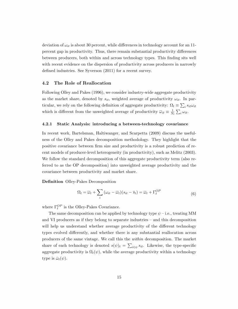
Definition Olley-Pakes Decomposition

Ωt = ωt +∑i

(ωit − ωt)(sit − st) = ωt + ΓOPt (6)

where ΓOPt is the Olley-Pakes Covariance.

The same decomposition can be applied by technology type ψ – i.e., treating MM

and VI producers as if they belong to separate industries – and this decomposition

will help us understand whether average productivity of the different technology

types evolved differently, and whether there is any substantial reallocation across

producers of the same vintage. We call this the within decomposition. The market

share of each technology is denoted s(ψ)t =∑

i∈ψ sit. Likewise, the type-specific

aggregate productivity is Ωt(ψ), while the average productivity within a technology

type is ωt(ψ).

15

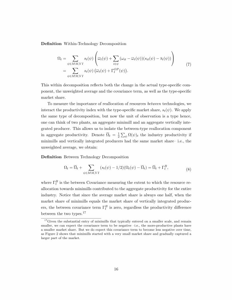
Definition Within-Technology Decomposition

Ωt =∑

ψ∈MM,V I

st(ψ)

ωt(ψ) +∑i∈ψ

(ωit − ωt(ψ))(sit(ψ)− st(ψ))

=

∑ψ∈MM,V I

st(ψ)(ωt(ψ) + ΓOPt (ψ)

).

(7)

This within decomposition reflects both the change in the actual type-specific com-

ponent, the unweighted average and the covariance term, as well as the type-specific

market share.

To measure the importance of reallocation of resources between technologies, we

interact the productivity index with the type-specific market share, st(ψ). We apply

the same type of decomposition, but now the unit of observation is a type hence,

one can think of two plants, an aggregate minimill and an aggregate vertically inte-

grated producer. This allows us to isolate the between-type reallocation component

in aggregate productivity. Denote Ωt = 12

∑ψ Ω(ψ)t the industry productivity if

minimills and vertically integrated producers had the same market share– i.e., the

unweighted average, we obtain:

Definition Between Technology Decomposition

Ωt = Ωt +∑

ψ∈MM,V I

(st(ψ)− 1/2)(Ωt(ψ)− Ωt) = Ωt + ΓBt , (8)

where ΓBt is the between Covariance measuring the extent to which the resource re-

allocation towards minimills contributed to the aggregate productivity for the entire

industry. Notice that since the average market share is always one half, when the

market share of minimills equals the market share of vertically integrated produc-

ers, the between covariance term ΓBt is zero, regardless the productivity difference

between the two types.17

17Given the substantial entry of minimills that typically entered on a smaller scale, and remainsmaller, we can expect the covariance term to be negative –i.e., the more-productive plants havea smaller market share. But we do expect this covariance term to become less negative over time,as Figure 2 shows that minimills started with a very small market share and gradually captured alarger part of the market.

16

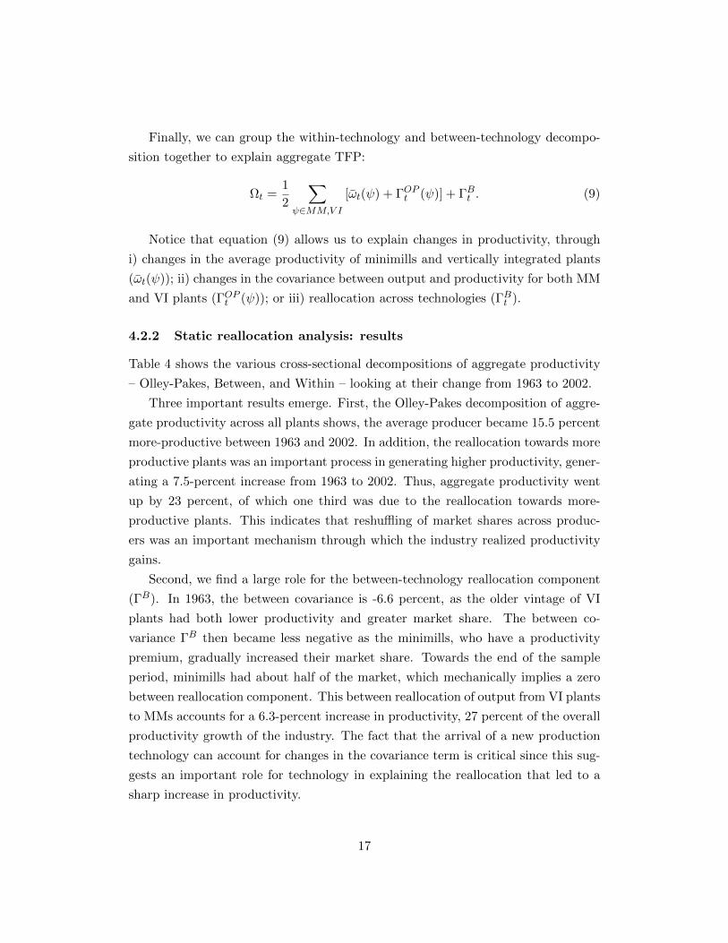
Finally, we can group the within-technology and between-technology decompo-

sition together to explain aggregate TFP:

Ωt =1

2

∑ψ∈MM,V I

[ωt(ψ) + ΓOPt (ψ)] + ΓBt . (9)

Notice that equation (9) allows us to explain changes in productivity, through

i) changes in the average productivity of minimills and vertically integrated plants

(ωt(ψ)); ii) changes in the covariance between output and productivity for both MM

and VI plants (ΓOPt (ψ)); or iii) reallocation across technologies (ΓBt ).

4.2.2 Static reallocation analysis: results

Table 4 shows the various cross-sectional decompositions of aggregate productivity

– Olley-Pakes, Between, and Within – looking at their change from 1963 to 2002.

Three important results emerge. First, the Olley-Pakes decomposition of aggre-

gate productivity across all plants shows, the average producer became 15.5 percent

more-productive between 1963 and 2002. In addition, the reallocation towards more

productive plants was an important process in generating higher productivity, gener-

ating a 7.5-percent increase from 1963 to 2002. Thus, aggregate productivity went

up by 23 percent, of which one third was due to the reallocation towards more-

productive plants. This indicates that reshuffling of market shares across produc-

ers was an important mechanism through which the industry realized productivity

gains.

Second, we find a large role for the between-technology reallocation component

(ΓB). In 1963, the between covariance is -6.6 percent, as the older vintage of VI

plants had both lower productivity and greater market share. The between co-

variance ΓB then became less negative as the minimills, who have a productivity

premium, gradually increased their market share. Towards the end of the sample

period, minimills had about half of the market, which mechanically implies a zero

between reallocation component. This between reallocation of output from VI plants

to MMs accounts for a 6.3-percent increase in productivity, 27 percent of the overall

productivity growth of the industry. The fact that the arrival of a new production

technology can account for changes in the covariance term is critical since this sug-

gests an important role for technology in explaining the reallocation that led to a

sharp increase in productivity.

17

Third, drilling down to the technology type, we see that minimills increased

their aggregate TFP (Ω(MM)) by ten percent, while vertically integrated plants

raised their aggregate TFP (Ω(V I)) by 24 percent. This “catching-up” of vertically

integrated producers mirrors the results in Table 3: While vertically integrated

producers were less productive than the minimills, by the end of the sample period,

they had almost completely caught up. Interestingly, the reason for this catch-up of

vertically integrated producers is not due to changes in the Olley-Pakes covariance

term ΓOPt (ψ), whose contribution to productivity growth is 5.2 percent for minimills

and 5.3 percent for vertically integrated producers. Rather, it was the much higher

increase in average plant productivity for vertically integrated producers (ωit(V I))

of 18.3 percent, versus a ωit(MM) of 4.8 percent for minimills.

Our analysis so far points to a large impact of minimill entry on shaping overall

industry productivity. We find that about 48 percent of total aggregate productivity

growth can directly be attributed to minimills, with 27 percent due to reallocation

away from the old technology and the remaining 21 percent due to productivity

improvements at minimill plants, which captures learning by doing taking place at

minimills.18

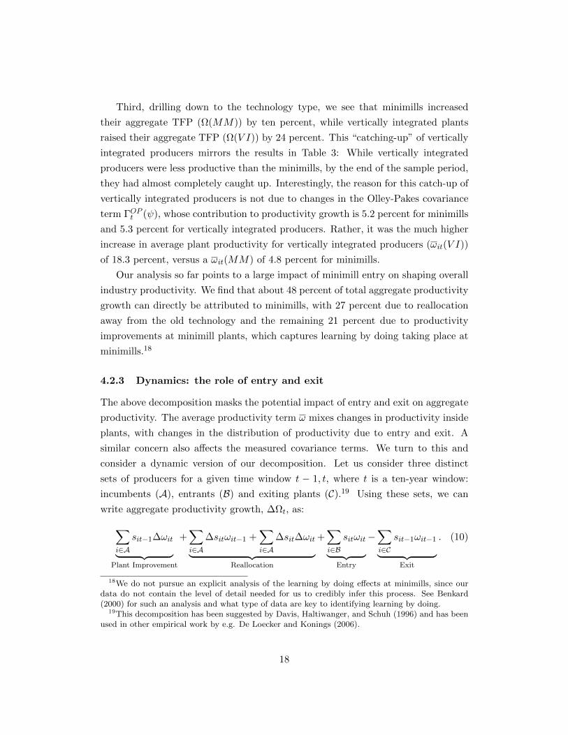
4.2.3 Dynamics: the role of entry and exit

The above decomposition masks the potential impact of entry and exit on aggregate

productivity. The average productivity term ω mixes changes in productivity inside

plants, with changes in the distribution of productivity due to entry and exit. A

similar concern also affects the measured covariance terms. We turn to this and

consider a dynamic version of our decomposition. Let us consider three distinct

sets of producers for a given time window t − 1, t, where t is a ten-year window:

incumbents (A), entrants (B) and exiting plants (C).19 Using these sets, we can

write aggregate productivity growth, ∆Ωt, as:∑i∈A

sit−1∆ωit︸ ︷︷ ︸Plant Improvement

+∑i∈A

∆sitωit−1 +∑i∈A

∆sit∆ωit︸ ︷︷ ︸Reallocation

+∑i∈B

sitωit︸ ︷︷ ︸Entry

−∑i∈C

sit−1ωit−1︸ ︷︷ ︸Exit

. (10)

18We do not pursue an explicit analysis of the learning by doing effects at minimills, since ourdata do not contain the level of detail needed for us to credibly infer this process. See Benkard(2000) for such an analysis and what type of data are key to identifying learning by doing.

19This decomposition has been suggested by Davis, Haltiwanger, and Schuh (1996) and has beenused in other empirical work by e.g. De Loecker and Konings (2006).

18

The first term is denoted Plant Improvement, the next two terms on are the

Reallocation terms, and the last two terms are the Entry and Exit components. The

above decomposition directly isolates the net-entry effect on aggregate productivity

by verifying the importance of the last two components in total productivity growth.

Finally, to isolate the role of entry and exit for both types of technology separately,

we expand the above by computing equation (10) by technology type ψ. When we

refer to the total impact of reallocation, we group all terms except for the plant-

improvement component.

Table 5 presents the decomposition across all plants and by technology.The first

row of Table 5 restates the 23-percent productivity growth in the U.S. steel sector,

but far faster growth for vertically integrated plants than for minimills.

Across the entire sample period, over which productivity increased by 23 percent

productivity growth, within plants accounted for a 10 percent increase in aggregate

productivity (or a 43 percent share), while reallocation and net entry are responsible

for the remainder. Thus, the total share of reallocation in aggregate productivity

growth, including both the reallocation induced by market-share reallocation across

incumbents and the net-entry process, is two-thirds.

A clear picture emerges when we move to the decomposition by technology.

The main driver of productivity growth for minimills is the within component of

14.7 percent, capturing the technological change in minimills. This is suggestive

of the substantial learning by doing that took place in minimill production– in

particular learning how to produce higher quality steel – over the sample period.

The reallocation component is negligible.

The same analysis of VI producers yields substantially different results: The

plant improvement component, of 10.2 percent, is smaller than that of minimills

(14.7 percent), the net entry term of 3.9 percent is almost 19 percent of total pro-

ductivity growth over the sample. Most noteworthy is that the reallocation term of

11.8 percent is responsible for 48 percent of industry-wide productivity growth.

In the last row of Table 5, we restate the distinct role of the net-entry process

across technologies. We present the productivity premium of entrants, compared

to the set of exiting plants. Across the entire sample period, VI entrants were

4.4 percent more productive than those VI plants that exited the industry. New

minimills, on the other hand, entered with no specific productivity advantage.

To summarize, we find a drastic difference in the role of reallocation between

technologies. The productivity growth of minimills is entirely due to common within-

19

plant productivity growth, whereas integrated producers’ productivity growth came

from the reallocation of resources across producers (67 percent). In the next section,

we focus on the role of reallocation among vertically integrated producers, which

was instrumental for the productivity growth among producers relying on the old

technology, and consequently triggered productivity growth for the industry as a

whole.

4.3 Catching up of the old technology

So far, we have shown that a substantial part of the industry’s productivity growth

can be accounted for by the arrival of the new technology and its own technological

progress, capturing about half of the productivity growth in the industry. The

entry of the new technology, however, spurred a dramatic reallocation process in

the incumbent technology leading to a sharp increase in productivity– where the

exit margin played a key role. It is, therefore, natural to ask how incumbents

became more productive. From our various decompositions we already know that

the exit of inefficient producers was a key driver, in addition to the reallocation

among existing producers.

To uncover the underlying mechanism, we incorporate the product space of the

industry. We know from Figure 6 that the market-share trajectories of minimills

for, broadly speaking, two product categories – bar products and sheet products

– were very different. Indeed, minimills took over bar products, but not sheet

products. Therefore we verify whether the substantial productivity gains among

(surviving) VI producers over our sample period were related to the product-market

competition – i.e., did VI producers of bar products exit, leaving only those VI

producers specializing in sheet products? In other words: How important was the

increased competition, due to minimill entry, for incumbents’s productive efficiency?

The distinction between the two product groups is relevant to the extent that

(1) there exists a productivity difference among bar and sheet producers, and (2)

survival is related to specialization.20 In order to verify whether this mechanism is

important in the data, we first test whether plants specializing in sheet products were,

on average, more productive, than those specializing in bar products. Subsequently,

20A potential third component would be the change in product specialization at the plant levelover time. However, we find very little change in product specialization over time; and thus thismechanism cannot generate within-plant productivity improvements. This finding sits well withour implicit assumption of plant-level productivity.

20

we ask whether the product specialization variable predicts plant survival. We run

both tests on the total sample of plants in our data, and on the subsample of VI

producers. In the latter, we compare plants of the same technology and verify

whether product specialization can explain the rapid productivity growth among

the group of VI producers.

Table 6 estimates both a technology and sheet-specialization productivity pre-

mium for a number of specifications, where sheet specialization refers to the share

of a plant’s revenue accounted for by sheet products.21 In Panel A, we consider all

plants in the industry, and find a robust and highly significant productivity advan-

tage for plants specializing in sheet products, while controlling for technology, and

an exhaustive set of fixed effects. Even if we compare plants of the same technology,

within the same firm and state, in the same year, we find a 12 percent productivity

premium for plants that completely specialized in sheet. In Panel B, we focus on the

VI producers, and find a similar premium. These results, therefore, strongly suggest

that the rapid productivity growth of VI producers was due to the reallocation from

bar to sheet producers. The latter is consistent with the market-share trajectories

presented in Figure 6, which showed MM taking over bar products but not sheet

products.

Taking the sheet productivity premium as given, we verify whether VI producers

producing primarily sheet products had a higher likelihood of survival. In Table 7,

we present survival regressions, where we run an indicator of plant survival – whether

a plant which was in active in 1963, survived until 2002 – against plant technology

and sheet specialization.22 In Panel A, we consider all plants in the industry and

find that the sheet specialization ratio variable has a strong positive impact on a

plant’s survival probability, holding fixed its technology. Indeed, a plant that was

fully specialized in sheet had a 31-percent-higher probability of surviving than a

plant that was fully specialized in bar. This is a very large effect, as plants have

a 33-percent likelihood of survival to begin with. Moreover, this effect is robust

to controlling for the plant’s capital and productivity– standard predictors of plant

21For all practical purposes, minimills do not produce sheet products. Moreover, there is littleyear-to-year variation in the share of revenues accounted for by sheet products within a plant. Thissuggests that it is difficult to alter the product mix at the plant level. Given the lack of within-plantvariation in sheet specialization, regressions with plant-level fixed effects will have little power toidentify the productivity premia of sheet producers.

22These results are robust to looking at survival from 1967, 1972 or even 1977, until 2002.Likewise, these results are also robust to looking at survival until 1997 and 1992.

21

survival.23

The productivity difference between sheet and bar producers is only relevant to

the extent that it exists among integrated producers. In Panel B, we focus on VI

producers and find a very similar effect: VI producers specializing in sheet products

in 1963 had a 31-percent-higher probability of surviving to the year 2002. We note

that predicting plant survival over a forty year period is a very demanding task.

Even when our sample size is reduced to 78 VI producers active in 1963, we obtain

a t-statistic of 1.6 on the sheet-specialization variable, while controlling for capital

and productivity.

Thus, the joint productivity and survival premium for sheet producers helps

explain the overall productivity growth of VI producers in the aftermath of minimill

entry. Minimills increased competition in the bar market, leading to the exit of

inefficient VI producers. As a consequence, the set of remaining VI producers was

more productive due to an increased concentration in the sheet product market.

This mechanism, therefore, manifests itself in substantially higher productivity of

VI producers and a dramatic drop of VI’s market share of bar products. In light of

our decomposition results, presented in Tables 4 and 5, 34 percent of the industry’s

productivity growth is due to the reallocation process among VI producers, in which

the specialization in sheet products seem to have played a crucial role. To obtain

the 34 percent contribution, we use the fact that 67 percent of the VI productivity

growth was due to reallocation (Table 5).

Finally, the only component we have not explained is the pure within-plant

productivity growth component for VI producers, which, according to our results

in Table 5, accounts for only 13 percent of aggregate TFP growth. This common

shift of the production frontier for VI producers captures the direct technological

innovations in steel making at integrated plants due to active investments, and

improvements in technical efficiency. Put another way, it would be surprising if

40 years of innovation in the engineering and management of vertically integrated

plants had not manifested itself in increased productivity. Still, this means that 87

percent of total productivity growth can be attributed to the reallocation induced

by minimill entry.

23See Collard-Wexler (2009) and the references therein.

22

4.4 Market Power and Reallocation

The drop in demand for U.S. steel producers and the variation in the market-shares

trajectories across products point to drastic changes in competition. We argued

that the entry of the minimill intensified competition for domestic steel producers,

in particular for the bar segment of the industry (see Section 4.3). In addition to

this increased domestic competition, it is well known that international competition

intensified through a substantial increase of imports. The increased competition is

expected to affect a plant’s residual demand curve and, therefore, impact its ability

to charge a price above marginal cost. The change in the residual demand elasticity,

and its associated markup response, are expected to affect the reallocation across

producers, as well.

We rely on our empirical framework to (1) show that markups indeed decreased

as competition increased, and (2) show how lower markups are directly related to

our measure of reallocation, the covariance of productivity and a plant’s market

share.

A nice feature of our approach is that we can generate measures of market power

from our estimates of the production function. We rely on our production function

framework to recover markups by technology type and plant. In order to obtain

markups from the plant-level production data, we follow the approach suggested

by De Loecker and Warzynski (2012). Appendix C.2 presents the details of this

approach. At the core of this approach lies the assumption that plants minimize

costs and that at least one input of production faces no adjustment costs.

The two main ingredients of computing markups are the output elasticity of in-

termediate inputs, such as materials and energy, and the corresponding expenditure

share of the input. The latter is directly observed in the data, whereas the out-

put elasticities are recovered after we estimate the production function as discussed

above.

We compute markups by technology as obtained from technology-specific ag-

gregate expenditures on an intermediate input (Et(ψ)), materials in our case, and

sales (Rt(ψ)) while relying on a time-invariant Cobb-Douglas output elasticity of

the intermediate input (βm):

µt(ψ) = βmRt(ψ)

Et(ψ). (11)

Under the commonly assumed Cobb-Douglas production function these markups

23

are in fact the correct technology-specific markups, with the markup by technology

thought of as a weighted average across plants where the weights are the expenditure

share on materials of a given plant in the total expenditures for plants of the same

technology.24 Figure 4 plots the markup trajectory over 40 years for both MM and

VI plants. Markups have steadily decreased over time and are consistent with the

drop in prices and external measures of concentration reported for the steel sector.

Markups were, on average, higher for minimills, confirming the results from the

augmented production function estimation in Table 3, and this is as expected since

they produce more efficiently while competing in the same product market.

Markups fell at the same time as the covariance between output and productivity

increases. Suppose that this fall in markups is due to a firms’ residual demand curve

becoming more elastic. In other words, markups fell because the product market

for steel became more competitive. This does not seem unlikely since there are far

more steel producers in 2002 than 1963 competing over a roughly similar market

size.25

A more elastic residual demand curve will accentuate the relationship between

productivity and output. Furthermore, the increase in the residual demand curve

for integrated firms is consistent with the increased competition from minimills and

a resulting decline in their market share. A similar point is made, in the context

of variable markups and trade liberalization, by Edmond, Midrigan, and Xu (2012)

and Mayer, Melitz, and Ottaviano (2011). Thus we expect the extent of competition

to be directly linked to reallocation, which is what we find in the data.

5 Alternative explanations and Robustness Analysis

In this section, we explore various alternatives that can potentially help explain the

sharp increase in productivity growth. It is important to note that these alterna-

tives are not mutual exclusive. The point of this section is not to argue that only

technology was responsible for bringing about the efficiency gains. We show that

our main results are not affected by controlling for these alternative explanations:

Firm-level characteristics, geography, and international trade do not appear to play

24To see this, use ciψt = EitEt(ψ)

in the share weighted markup expression for a type ψ, where ciψt

is the share of an individual plant in the type’s total: µt(ψ) =∑i∈ψ ciψtµit =

∑i∈ψ ciψtβm

RitEit

=

βmRt(ψ)Et(ψ)

.25Total production in 1965 was about 130 million, and by 2000 is about 112 million tons. Also

see Figure 1 where the value of production as well as the number of plants are presented

24

a role in explaining either the differences in productivity between minimills and

vertically integrated producers, or the reallocation between these technologies.

Finally, we present the main results from our decomposition analysis using a

variety of productivity estimates (as presented in Table 3). We discuss the robust-

ness of our results, and highlight the importance of our corrections in establishing

a prominent role of technology in generating aggregate productivity growth.

5.1 Management practices and ownership

Our analysis, thus far, has been focused on plants. To the extent that better plants

are managed by better firms, we are potentially attributing productivity differences

across plants to technology, where it might simply reflect that more-productive

plants, regardless which technology they use, are better-managed or belong to more

efficiently organized firms. The potential role for firm-level variables explaining pro-

ductivity differences is, in particular, plausible given the recent findings of Bloom

and Van Reenen (2010). They present empirical evidence that measures of pro-

ductivity, like the one we use, are correlated with various management practices,

reflecting human resource (HR) practices and organizational design. Ichniowski,

Shaw, and Prennushi (1997) find that better HR practices lead to higher productiv-

ity using detailed product-line data. Their results confirm recent theoretical models

that stress the importance of complementarities among work practices.

To check whether the minimill premium in our sample period was not driven by

better-managed firms, or any particular kind of firm-specific ownership structure,

we compare minimills to VI plants within the same firm and time period using by

regressing productivity on technology, and a firm-year fixed effect. Table 8 presents

these results. We start out in column I with a base premium of ten percent. We

find an almost identical productivity premium, of around ten percent, for minimills

when including a firm-time fixed effect (column II).

These results suggest that the minimill productivity premium was not driven

by a particular allocation of minimill plants to more-productive firms with, say,

better management or human resource (HR) practices. Moreover, our results do

not contradict those presented by Ichniowski, Shaw, and Prennushi (1997), who

rely on a sample of 17 rolling mills collocated with vertically integrated plants in

the United States and, therefore, omit minimills from the analysis. Thus, there is

no information on the relative performance of minimills. In addition, they focus on

25

rolling operations, which we purposefully leave out.26

Finally, including firm fixed effects does not rule out an effect of management.

If management practices differ between plants at the same firm, and these intra-

firm differences in management are precisely aligned with the technology used in

production, then we could still attribute management effects to minimills. However,

while we think that this story is very unlikely, it would take historical plant-level

data on management to rule it out, and, Census data during our sample period do

not track this type of information.27

5.2 Geography

Although steel production has historically been concentrated in a few regions in the

U.S., there is still considerable variation of activity across regions. In 2002, 63 per-

cent of steel was produced in the Midwest – i.e., Illinois, Indiana, Michigan, Ohio,

and Pennsylvania – while this figure was 75 percent in 1963. We check whether

regional patterns influence our results by incorporating a full set of state-year dum-

mies, in a regression of productivity on our measure of technology. Table 8 shows

that the substantial minimill premium is largely unaffected when including state-

time fixed effects. This result reflects that minimills are, on average, 12.9 percent

more productive than integrated producers in the same state and year (column

III). Furthermore, this result is robust with respect to including technology-year

interactions.

Finally, in column IV, we include a joint firm-state-year fixed effect and find that

the technology premium is still strongly positive and significant, but with a point

estimate of 25 percent. This suggests that minimills are vastly more productive,

even when we compare a minimill and a vertically integrated plant owned by the

same firm, and located in the same state. The results in Table 8 indicate that the

productivity premium for minimills is extremely robust, and is not an artifact of a

particular selection mechanism at the firm or regional level, or an interplay of both.

26The main reason to omit rolling mills is because the boundary between rolling operations andother steel shaping operations, such as pipe making or other more artisanal iron work, is less clear.By focusing on the production of molten steel, we obtain a sharper definition of the industry.

27The new wave of economic Census will contain a Management and Organization PracticesSurvey (MOPS). See World Management Survey and http://bhs.econ/census.gov/bhs/mops/

for more on this recent addition.

26

5.3 International Trade

It is well documented that the U.S. steel sector has faced stronger competition

from foreign producers over the course of the last four decades. However, for our

purposes, the relevant question is whether the mere increase in import competition

could explain the rapid productivity growth in the industry.

Table 9 lists the average productivity growth and import penetration ratio across

the US manufacturing industries (4-digit SIC codes), and compares them with the

steel industry. The upper panel lists the absolute imports and shows that the

steel sector’s imports did not increase nearly as much as the modal manufacturing

industry.

The bottom panel reports the import penetration ratio and highlights that in-

ternational competition increased across all U.S. manufacturing industries, and that

steel was no exception. However, both in an unweighted and weighted sense, the

change in international competition for U.S. steel was lower than the average across

all sectors of US manufacturing. Productivity growth in the steel industry, as docu-

mented previously in Table 1, has been three times higher than the average. While

we see increased import competition for domestic steel producers, this, by itself,

cannot explain the exceptional improvements in productivity.

Using the statistical relationship between productivity growth and the change

in the import penetration ratio, over the period 1972-1996, we would predict only

an eight percent productivity growth for the steel industry.28 Put differently: The

change in international competition can explain at most one third of the productivity

growth.

These types of estimates are further subject to various biases and measurement

problems. For instance, the Semiconductor industry experienced remarkable pro-

ductivity growth, while its import penetration ratio increased as well. However, the

import surge was due to U.S. producers outsourcing production while focusing on

R&D and design in the U.S. affiliates. Identifying the impact of foreign competi-

tion on industry performance is further complicated due to endogenous changes in

28We construct a matched production-trade database at the 4-digit SIC87 level using the NBERManufacturing Database and the U.S. Trade Database. We consider a simple long difference re-gression of TFP growth on the change in the import penetration ratio. The estimated coefficientsare used to predict the steel industry’s productivity growth. Specifically, we run the following re-gression: ∆ΩI = γ0 + γ1∆IPRI + νI across the entire sample of 4-digit SIC87 industries, where ∆is the difference over the 1972-1996 period, and we weigh observations by the industry’s share intotal manufacturing production.

27

international competition, as well as to reversed causality from productivity growth

to international trade.

In this paper, we focus on a clean and directly measurable source of productivity

growth: the arrival of a new technology. The potential role of international trade

in affecting productivity growth indirectly is further weakened since the specific

trajectory of imports, or any alternative measure of international competition, is

not aligned with the arrival of the new technology. We do acknowledge, as shown in

Table 9, that changes in international competition did most likely affect domestic

producers by shifting in the residual demand for steel products. In this sense,

the increased competition introduced by minimills was reinforced, if anything, by

competing over a smaller market share, a mechanism we account for in our analysis

of markups.

Finally, one might still worry that the effects of international competition were

more pronounced for integrated producers than for minimills, thereby affecting the

interpretation of our results. Therefore, we checked whether the measures of inter-

national competition, such as import shares, differed across products. As discussed

previously, minimills were mainly active in the bar segment, especially in the period

1972-1996, where we observe good measures of international competition (also see

Figure 2). When we break down imports and exports by product, we find that

imports show a rise for bar products produced by minimills that is similar to that

of sheet products, which minimills do not produce.

In addition, since minimills were historically more concentrated in the midwest,

while integrated producers were active in coastal areas, we might worry that min-

imills were more insulated from foreign competition due to substantial intranational

shipping costs. However, in the previous subsection we discussed the robust pro-

ductivity advantage of minimills when controlling for regional differences.

5.4 Importance of Corrections and Robustness

Tables 10 and 11 presents robustness checks on our main decompositions of aggre-

gate productivity growth, both static and dynamic. For each of the productivity

estimates obtained using the specifications listed in Table 3, we produce the static

and dynamic decompositions.

The first column of Tables 10 and 11 rely on productivity estimates obtained

using the production function coefficients of specification VI in Table 3. We contrast

these to results obtained using productivity estimates obtained without correcting

28

for unobserved price differences across producers, and to results obtained without

correcting for simultaneity and selection. To assess the precision of our results, we

include bootstrapped confidence intervals on the share of each component for all

decompositions.

5.4.1 Robustness

We find that our decompositions are qualitatively robust to alternative specifications

of the production function. We find similar differences in the speed of productivity

growth between technologies, a far larger role for reallocation among the vertically

integrated producers than among the minimills, and a large role for the between

covariance in productivity growth.

The various components of the decompositions use plant-level estimates of pro-

ductivity, which rely on estimated production function coefficients, and thus are also

estimates. We use a block bootstrap routine to produce confidence intervals of the

shares of each component. The 95 percent confidence intervals around the various

shares are reasonably tight.29 For example the confidence interval around aggregate

productivity growth is similar across all specifications.

5.4.2 Importance of Corrections

The results in Tables 10 and 11, also point out the importance of correcting for

unobserved productivity and price errors when estimating the production function,

to obtain the correct quantitative effects of the entry of minimills on aggregate

productivity. What is particularly sensitive to the specification of the production

function is the between decomposition. Indeed, the between component is 27 per-

cent in Column VI (GMM and price correction), as opposed to 11 percent using

OLS productivity estimates in Column I (OLS). These differences are statistically

significant as the confidence intervals for the between share do not overlap between

these two columns. This is not too surprising, as Table 3 showed that the minimill

productivity premium was far larger in Column VI, than in Column I. These differ-

ence in the estimated productivity advantages of minimills directly spill over to the

estimated magnitude of the between covariance. Further controlling for differences

in input price trends across plants does not change the results.

29As far as we know, this is the first paper to produce confidence intervals around the componentsof the decomposition of (an industry’s) aggregate productivity, and we cannot compare our resultsto existing work.

29

The role of entry and exit is altered by omitting to correct for price and produc-

tivity errors in the production function. The impact of the exit process of integrated

producers is cut in half (from 19 to 8 percent between Column VI and I), while the

within-plant minimill improvements are underestimated (107 versus 79 percent from

Column VI to I). These findings echo the results of Foster, Haltiwanger, and Syver-

son (2008): Correcting for variation in plant-level prices is crucial to obtain reliable

productivity measures, and more importantly, to measure the impact of entry and

exit, an important part of our reallocation mechanism, on aggregate productivity.

Summing up, if we incorrectly ignored price variation across producers, the en-

dogeneity of inputs and the non-random exit of plants in the data, we would under-

estimate the reallocation mechanism by a factor of two. Our results suggest that the

total effect of minimill entry on industry-wide productivity growth was 87 percent.

This share drops to about 72 percent when ignoring unobserved price and produc-

tivity heterogeneity. However, although we find a much larger magnitude, the role

of technology is present when using uncorrected productivity estimates, which adds

to the robustness of the importance of our specific reallocation mechanism.

6 Conclusion

There is by now extensive evidence that reallocation of resources across producers

substantially impacts productivity growth. This paper is one of the first to provide

a specific mechanism underlying such a reallocation: The entry of a new technology,

and its associated increased competition, were largely responsible for the massive

productivity growth in the U.S. steel industry.

We provide evidence that technological change can, by itself, bring about a

process of resource reallocation over a long period of time and lead to substantial

productivity growth for the industry as a whole. We find that the introduction of a

new production technology spurred productivity growth through two channels.

First, the entry of minimills lead to a slow but steady drop in the market share

of the incumbent technology, the vertically integrated producers. As minimills were

11 percent more productive, this movement of market share between technologies

was responsible for a third of the industry’s productivity growth. Second, while the

new technology started out with a 25 percent productivity premium, by the end of

the sample, minimills and vertically integrated producers were very similar in terms

of efficiency. This catching-up process of the incumbents came about from a large

30

within reallocation of resources among vertically integrated plants.

The reallocation among vertically integrated plants was largely due the exit

of inefficient producers active in the low-quality segment (bar products.) On the

other hand, minimills’s productivity increased gradually over time due to a shift

in the production function for all minimill producers. Although the first mimimill,

producing at a commercial level, entered in the late fifties, the productivity effects

were long-lasting and still affect the industry’s performance today. In fact, the

recent trend in market shares suggests that minimills started to enter the high-

quality segment of the industry – sheet products – and taking our results at face

value would indicate that more substantial productivity gains are expected.

Our results indicate that the arrival of new technologies can have a major impact

on productive efficiency through increased competition and its associated realloca-

tion of economic resources, leading to an increase in the industry’s overall perfor-

mance. It is critical to obtain measures of plant-level performance and technology

to identify this mechanism – i.e., without indicators of technology at the plant-level,

we would falsely attribute the productivity gains to other factors correlated with

aggregate productivity, such as international competition, geography, and a variety

of firm-level characteristics.

References

Ackerberg, D., L. Benkard, S. Berry, and A. Pakes (2007): “EconometricTools for Analyzing Market Outcomes,” in Handbook of Econometrics, ed. byJ. Heckman, and E. Leamer, vol. 6a, chap. 63, pp. 4171–4276. Elsevier.

Ackerberg, D., G. Frazer, and K. Caves (2006): “Structural Estimation ofProduction Function,” Working Paper UCLA.

American Iron and Steel Institute (2010): Annual Statistical Report of theAmerican Iron and Steel Institute. Washington D.C.

Bartelsman, E., R. Becker, and W. Gray (2000): “Nber-ces manufacturingindustry database,” Last accessed May, 25, 2006.

Bartelsman, E., J. Haltiwanger, and S. Scarpetta (2009): “Cross-countrydifferences in productivity: the role of allocation and selection,” Discussion paper,NBER Working Paper.

Benkard, C. (2000): “Learning and Forgetting: The Dynamics of Aircraft Pro-duction,” American Economic Review, 90(4), 1034–1054.

31

Bernard, A., J. Jensen, and P. Schott (2006): “Survival of the best fit: Expo-sure to low-wage countries and the (uneven) growth of US manufacturing plants,”Journal of International Economics, 68(1), 219–237.

Bloom, N., B. Eifert, A. Mahajan, D. McKenzie, and J. Roberts (2011):“Does management matter? Evidence from India,” Discussion paper, NationalBureau of Economic Research.

Bloom, N., and J. Van Reenen (2010): “Why do management practices differacross firms and countries?,” The Journal of Economic Perspectives, pp. 203–224.

Bresnahan, T. F., and D. M. G. Raff (1991): “Intra-Industry Heterogeneityand the Great Depression: The American Motor Vehicles Industry, 1929-1935,”The Journal of Economic History, 51(2), 317–331.

Collard-Wexler, A. (2009): “Productivity Dispersion and Plant Selection inthe Ready-Mix Concrete Industry,” Working Paper, New York University.

Crandall, R. (1981): The US steel industry in recurrent crisis: policy options ina competitive world. Brookings Institution Press.

Davis, S. J., J. C. Haltiwanger, and S. Schuh (1996): Job creation and de-struction. MIT Press Cambridge, Mass.

De Loecker, J. (2011): “Product Differentiation, Multiproduct Firms, and Esti-mating the Impact of Trade Liberalization on Productivity,” Econometrica, 79(5),1407–1451.

De Loecker, J., P. Goldberg, A. Khandelwal, and N. Pavcnik (2012):“Prices, Markups and Trade Reform,” Discussion paper, National Bureau of Eco-nomic Research.

De Loecker, J., and J. Konings (2006): “Job reallocation and productivitygrowth in a post-socialist economy: Evidence from Slovenian manufacturing,”European Journal of Political Economy, 22(2), 388–408.

De Loecker, J., and F. Warzynski (2012): “Markups and firm-level exportstatus,” American Economic Review, 102(6), 2437–2471.

Edmond, C., V. Midrigan, and D. Xu (2012): “Competition, markups, and thegains from international trade,” Discussion paper, National Bureau of EconomicResearch.

Foster, L., J. Haltiwanger, and C. Krizan (2001): “Aggregate productivitygrowth. Lessons from microeconomic evidence,” in New developments in produc-tivity analysis. University of Chicago Press.

32

Foster, L., J. Haltiwanger, and C. Syverson (2008): “Reallocation, FirmTurnover, and Efficiency: Selection on Productivity or Profitability?,” AmericanEconomic Review, 98(1), 394–425.

Fruehan, R. (1998): The Making, Shaping and Treating of Steel - 11th Edition.AISE Steel Foundation, Pittsburgh, USA.

Giarratani, F., G. Gruver, and R. Jackson (2007): “Clusters, agglomeration,and economic development potential: empirical evidence based on the adventof slab casting by US steel minimills,” Economic Development Quarterly, 21(2),148–164.

Hall, C. (1997): Steel phoenix: The fall and rise of the US steel industry. PalgraveMacmillan.

Hoerr, J. (1988): And the wolf finally came: The decline of the American steelindustry. University of Pittsburgh Press Pittsburgh.

Hortacsu, A., and C. Syverson (2004): “Cementing Relationships: VerticalIntegration, Foreclosure, Productivity, and Prices,” .

Ichniowski, C., K. Shaw, and G. Prennushi (1997): “The Effects of HumanResource Management Practices on Productivity: A Study of Steel FinishingLines,” American Economic Review, 87(3), 291–313.

Jarmin, R., S. Klimek, and J. Miranda (2009): “The Role of Retail Chains:National, Regional and Industry Results,” in Producer Dynamics: New Evidencefrom Micro Data, pp. 237–262. University of Chicago Press.

Mayer, T., M. Melitz, and G. Ottaviano (2011): “Market size, competition,and the product mix of exporters,” Discussion paper, National Bureau of Eco-nomic Research.

Melitz, M. (2003): “The Impact of Trade on Intra-Industry Reallocations andAggregate Industry Productivity,” Econometrica, 71(6), 1695–1725.

Olley, G. S., and A. Pakes (1996): “The dynamics of productivity in the telecom-munications equipment industry,” Econometrica, 64(6), 35.

Oster, S. (1982): “The Diffusion of Innovation among Steel Firms: The BasicOxygen Furnace,” The Bell Journal of Economics, 13(1), pp. 45–56.

Rogers, R. (2009): An economic history of the American steel industry. Taylor &Francis.

Schmitz, J. (2005): “What determines productivity? Lessons from the dramaticrecovery of the US and Canadian iron ore industries following their early 1980scrisis,” Journal of Political Economy, 113(3), 582–625.

33

Syverson, C. (2011): “What Determines Productivity?,” Journal of EconomicLiterature, 49(2), 326–65.

Van Biesebroeck, J. (2003): “Productivity dynamics with technology choice: Anapplication to automobile assembly,” The Review of Economic Studies, 70(1),167–198.

34

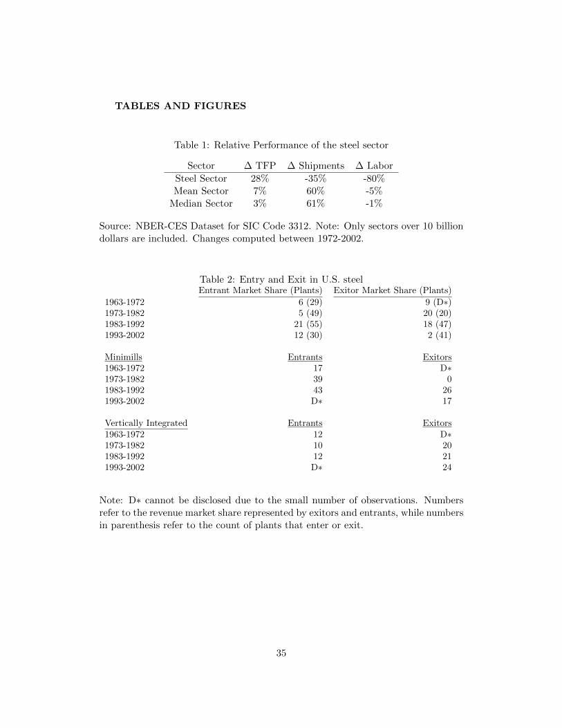
TABLES AND FIGURES

Table 1: Relative Performance of the steel sector

Sector ∆ TFP ∆ Shipments ∆ Labor

Steel Sector 28% -35% -80%Mean Sector 7% 60% -5%

Median Sector 3% 61% -1%

Source: NBER-CES Dataset for SIC Code 3312. Note: Only sectors over 10 billiondollars are included. Changes computed between 1972-2002.

Table 2: Entry and Exit in U.S. steelEntrant Market Share (Plants) Exitor Market Share (Plants)

1963-1972 6 (29) 9 (D∗)1973-1982 5 (49) 20 (20)1983-1992 21 (55) 18 (47)1993-2002 12 (30) 2 (41)

Minimills Entrants Exitors1963-1972 17 D∗1973-1982 39 01983-1992 43 261993-2002 D∗ 17

Vertically Integrated Entrants Exitors1963-1972 12 D∗1973-1982 10 201983-1992 12 211993-2002 D∗ 24

Note: D∗ cannot be disclosed due to the small number of observations. Numbersrefer to the revenue market share represented by exitors and entrants, while numbersin parenthesis refer to the count of plants that enter or exit.

35

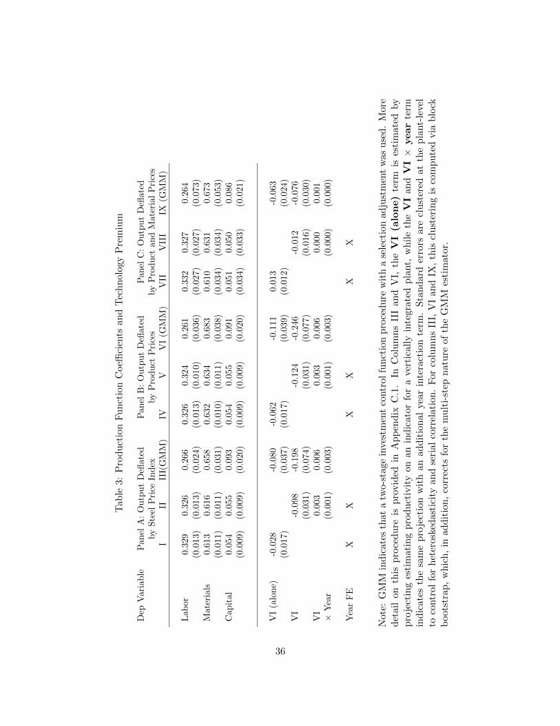
Tab

le3:

Pro

du

ctio

nF

un

ctio

nC

oeffi

cien

tsan

dT

ech

nol

ogy

Pre

miu

m

Dep

Var

iab

leP

anel

A:

Ou

tpu

tD

eflat

edP

an

elB

:O

utp

ut

Defl

ate

dP

an

elC

:O

utp

ut

Defl

ate

dby

Ste

elP

rice

Ind

exby

Pro

du

ctP

rice

sby

Pro

du

ctan

dM

ate

rial

Pri

ces

III

III(

GM

M)

IVV

VI

(GM

M)

VII

VII

IIX

(GM

M)

Lab

or0.

329

0.32

60.

266

0.3

26

0.3

24

0.2

61

0.3

32

0.3

27

0.2

64

(0.0

13)

(0.0

13)

(0.0

24)

(0.0

13)

(0.0

10)

(0.0

36)

(0.0

27)

(0.0

27)

(0.0

73)

Mat

eria

ls0.

613

0.61

60.

658

0.6

32

0.6

34

0.6

83

0.6

10

0.6

31

0.6

73

(0.0

11)

(0.0

11)

(0.0

31)

(0.0

10)

(0.0

11)

(0.0

38)

(0.0

34)

(0.0

34)

(0.0

53)

Cap

ital

0.05

40.

055

0.09

30.0

54

0.0

55

0.0

91

0.0

51

0.0

50

0.0

86

(0.0

09)

(0.0

09)

(0.0

20)

(0.0

09)

(0.0

09)

(0.0

20)

(0.0

34)

(0.0

33)

(0.0

21)

VI

(alo

ne)

-0.0

28-0

.080

-0.0

62

-0.1

11

0.0

13

-0.0

63

(0.0

17)

(0.0

37)

(0.0

17)

(0.0

39)

(0.0

12)

(0.0

24)

VI

-0.0

98-0

.198

-0.1

24

-0.2

46

-0.0

12

-0.0

76

(0.0

31)

(0.0

74)

(0.0

31)

(0.0

77)

(0.0

16)

(0.0

30)

VI

0.00

30.

006

0.0

03

0.0

06

0.0

00

0.0

01

×Y

ear

(0.0

01)

(0.0

03)

(0.0

01)

(0.0

03)

(0.0

00)

(0.0

00)

Yea

rF

EX

XX

XX

X

Not

e:G

MM

ind

icat

esth

ata

two-s

tage

inves

tmen

tco

ntr

olfu

nct

ion

pro

ced

ure

wit

ha

sele

ctio

nad

just

men

tw

asu

sed

.M

ore

det

ail

on

this

pro

ced

ure

ispro

vid

edin

Ap

pen

dix

C.1

.In

Col

um

ns

III

and

VI,

the

VI

(alo

ne)

term

ises

tim

ated

by

pro

ject

ing

esti

mat

ing

pro

du

ctiv

ity

onan

ind

icat

orfo

ra

ver

tica

lly

inte

grat

edp

lant,

wh

ile

the

VI

and

VI×

year

term

ind

icate

sth

esa

me

pro

ject

ion

wit

han

add

itio

nal

yea

rin

tera

ctio

nte

rm.

Sta

nd

ard

erro

rsar

ecl

ust

ered

atth

ep

lant-

leve

lto

contr

olfo

rh

eter

oske

dast

icit

yan

dse

rial

corr

elat

ion

.F

orco

lum

ns

III,

VI

and

IX,

this

clu

ster

ing

isco

mp

ute

dvia

blo

ckb

oot

stra

p,

wh

ich

,in

add

itio

n,

corr

ects

for

the

mu

lti-

step

nat

ure

ofth

eG

MM

esti

mat

or.

36

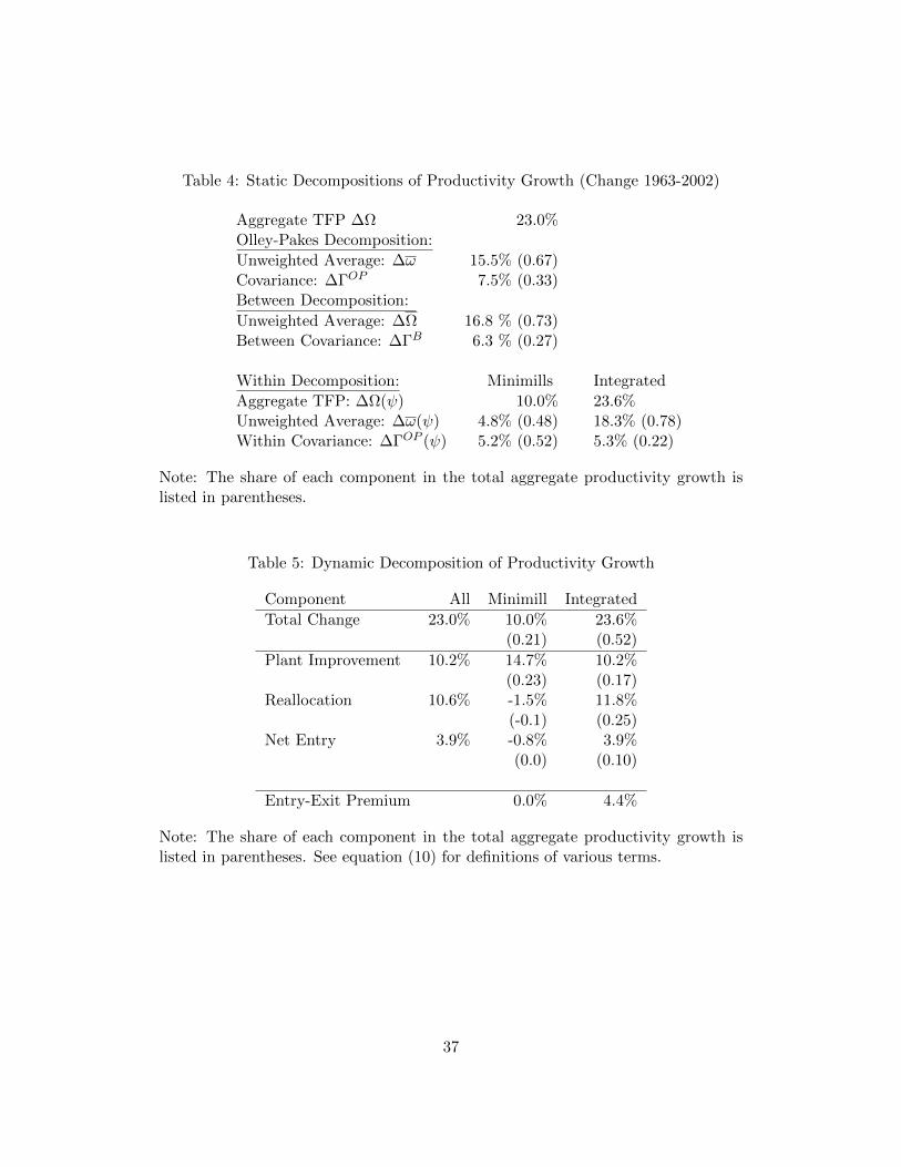
Table 4: Static Decompositions of Productivity Growth (Change 1963-2002)

Aggregate TFP ∆Ω 23.0%Olley-Pakes Decomposition:

Unweighted Average: ∆ω 15.5% (0.67)Covariance: ∆ΓOP 7.5% (0.33)Between Decomposition:

Unweighted Average: ∆Ω 16.8 % (0.73)Between Covariance: ∆ΓB 6.3 % (0.27)

Within Decomposition: Minimills Integrated

Aggregate TFP: ∆Ω(ψ) 10.0% 23.6%Unweighted Average: ∆ω(ψ) 4.8% (0.48) 18.3% (0.78)Within Covariance: ∆ΓOP (ψ) 5.2% (0.52) 5.3% (0.22)

Note: The share of each component in the total aggregate productivity growth islisted in parentheses.

Table 5: Dynamic Decomposition of Productivity Growth

Component All Minimill Integrated

Total Change 23.0% 10.0% 23.6%(0.21) (0.52)

Plant Improvement 10.2% 14.7% 10.2%(0.23) (0.17)

Reallocation 10.6% -1.5% 11.8%(-0.1) (0.25)

Net Entry 3.9% -0.8% 3.9%(0.0) (0.10)

Entry-Exit Premium 0.0% 4.4%

Note: The share of each component in the total aggregate productivity growth islisted in parentheses. See equation (10) for definitions of various terms.

37

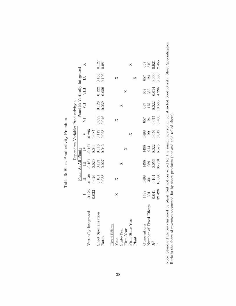
Tab

le6:

Sh

eet

Pro

du

ctiv

ity

Pre

miu

m

Dep

end

ent

Vari

ab

le:

Pro

du

ctiv

ityω

Pan

elA

:A

llP

lants

Pan

elB

:V

erti

call

yIn

tegra

ted

III

III

IVV

VI

VII

VII

IIX

XV

erti

call

yIn

tegr

ated

-0.1

26-0

.138

-0.1

67

-0.1

27

-0.2

95

0.02

20.0

26

0.0

20

0.0

44

0.0

87

Sh

eet

Sp

ecia

liza

tion

0.1

01

0.1

21

0.1

18

0.1

19

0.0

99

0.1

28

0.1

22

0.1

65

0.1

27

Rat

io0.0

38

0.0

27

0.0

42

0.0

68

0.0

46

0.0

39

0.0

59

0.1

06

0.0

81

Fix

edE

ffec

tsY

ear

XX

XX

Sta

te-Y

ear

XX

Fir

m-Y

ear

XX

Fir

m-S

tate

-Yea

rX

XP

lant

X

Ob

serv

atio

ns

149

81498

1498

1498

1498

657

657

657

657

657

Nu

mb

erof

Fix

edE

ffec

ts30

1301

289

914

129

124

175

353

124

540

R2

0.04

10.1

04

0.0

56

0.0

22

0.0

56

0.0

77

0.0

22

0.0

14

0.0

60

0.0

21

F32

.428

16.0

86

35.7

01

6.5

75

6.0

42

6.4

60

10.5

85

4.2

95

3.6

86

2.4

55

Not

e:S

tan

dar

dE

rror

scl

ust

ered

by

pla

nt,

bu

tn

ot

corr

ecte

dfo

rth

esa

mp

lin

ger

ror

inco

nst

ruct

edp

rod

uct

ivit

y.S

hee

tS

pec

iali

zati

on

Rat

iois

the

shar

eof

reve

nu

esac

cou

nte

dfo

rby

shee

tp

rod

uct

s(h

ot

an

dco

ldro

lled

shee

t).

38

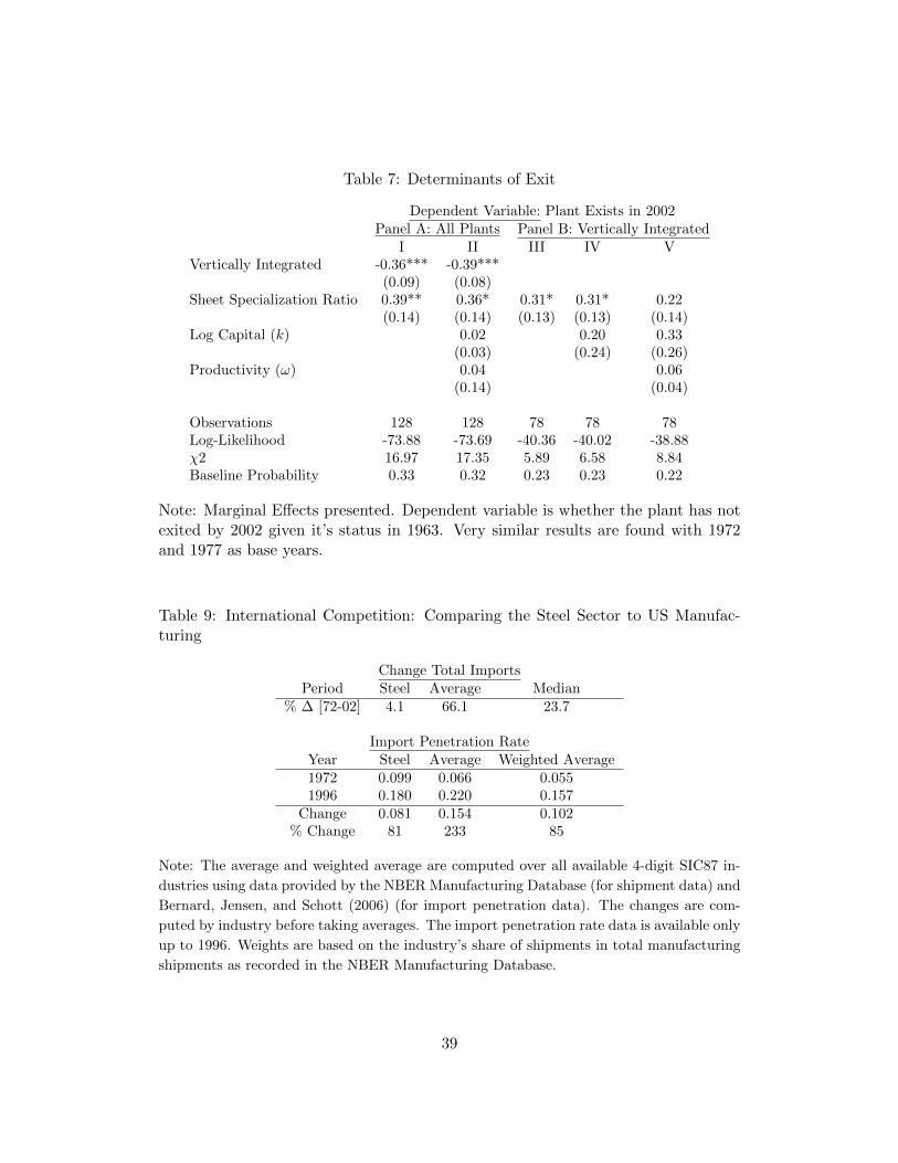
Table 7: Determinants of Exit

Dependent Variable: Plant Exists in 2002Panel A: All Plants Panel B: Vertically Integrated

I II III IV VVertically Integrated -0.36*** -0.39***

(0.09) (0.08)Sheet Specialization Ratio 0.39** 0.36* 0.31* 0.31* 0.22

(0.14) (0.14) (0.13) (0.13) (0.14)Log Capital (k) 0.02 0.20 0.33

(0.03) (0.24) (0.26)Productivity (ω) 0.04 0.06

(0.14) (0.04)

Observations 128 128 78 78 78Log-Likelihood -73.88 -73.69 -40.36 -40.02 -38.88χ2 16.97 17.35 5.89 6.58 8.84Baseline Probability 0.33 0.32 0.23 0.23 0.22

Note: Marginal Effects presented. Dependent variable is whether the plant has notexited by 2002 given it’s status in 1963. Very similar results are found with 1972and 1977 as base years.

Table 9: International Competition: Comparing the Steel Sector to US Manufac-turing

Change Total ImportsPeriod Steel Average Median

% ∆ [72-02] 4.1 66.1 23.7

Import Penetration RateYear Steel Average Weighted Average1972 0.099 0.066 0.0551996 0.180 0.220 0.157

Change 0.081 0.154 0.102% Change 81 233 85

Note: The average and weighted average are computed over all available 4-digit SIC87 in-

dustries using data provided by the NBER Manufacturing Database (for shipment data) and

Bernard, Jensen, and Schott (2006) (for import penetration data). The changes are com-

puted by industry before taking averages. The import penetration rate data is available only

up to 1996. Weights are based on the industry’s share of shipments in total manufacturing

shipments as recorded in the NBER Manufacturing Database.

39

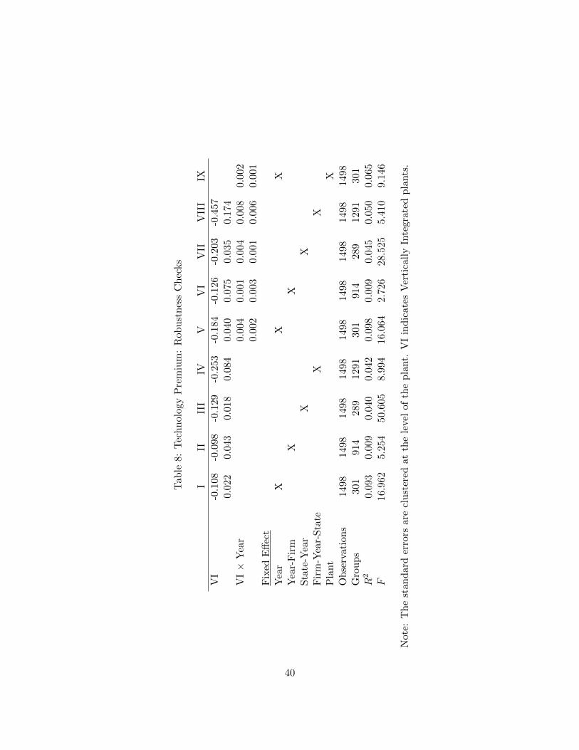
Tab

le8:

Tec

hn

olog

yP

rem

ium

:R

obu

stn

ess

Ch

ecks

III

III

IVV

VI

VII

VII

IIX

VI

-0.1

08-0

.098

-0.1

29-0

.253

-0.1

84-0

.126

-0.2

03-0

.457

0.02

20.

043

0.01

80.

084

0.04

00.

075

0.03

50.

174

VI×

Yea

r0.

004

0.00

10.

004

0.00

80.

002

0.00

20.

003

0.00

10.

006

0.00

1F

ixed

Eff

ect

Yea

rX

XX

Yea

r-F

irm

XX

Sta

te-Y

ear

XX

Fir

m-Y

ear-

Sta

teX

XP

lant

XO

bse

rvat

ion

s14

98

1498

1498

1498

1498

1498

1498

1498

1498

Gro

up

s301

914

289

1291

301

914

289

1291

301

R2

0.09

30.

009

0.04

00.

042

0.09

80.

009

0.04

50.

050

0.06

5F

16.9

625.

254

50.6

058.

994

16.0

642.

726

28.5

255.

410

9.14

6

Not

e:T

he

stan

dar

der

rors

are

clu

ster

edat

the

leve

lof

the

pla

nt.

VI

ind

icat

esV

erti

call

yIn

tegr

ated

pla

nts

.

40

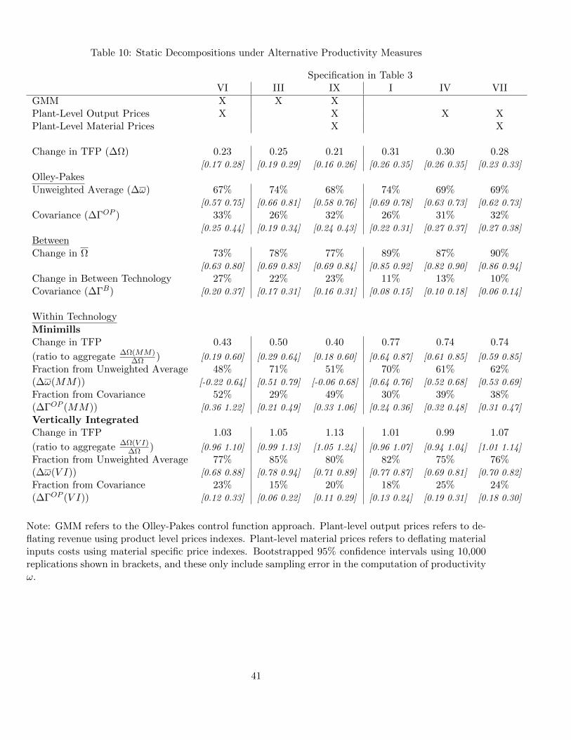
Table 10: Static Decompositions under Alternative Productivity Measures

Specification in Table 3VI III IX I IV VII

GMM X X XPlant-Level Output Prices X X X XPlant-Level Material Prices X X

Change in TFP (∆Ω) 0.23 0.25 0.21 0.31 0.30 0.28[0.17 0.28] [0.19 0.29] [0.16 0.26] [0.26 0.35] [0.26 0.35] [0.23 0.33]

Olley-Pakes

Unweighted Average (∆ω) 67% 74% 68% 74% 69% 69%[0.57 0.75] [0.66 0.81] [0.58 0.76] [0.69 0.78] [0.63 0.73] [0.62 0.73]

Covariance (∆ΓOP ) 33% 26% 32% 26% 31% 32%[0.25 0.44] [0.19 0.34] [0.24 0.43] [0.22 0.31] [0.27 0.37] [0.27 0.38]

Between

Change in Ω 73% 78% 77% 89% 87% 90%[0.63 0.80] [0.69 0.83] [0.69 0.84] [0.85 0.92] [0.82 0.90] [0.86 0.94]

Change in Between Technology 27% 22% 23% 11% 13% 10%Covariance (∆ΓB) [0.20 0.37] [0.17 0.31] [0.16 0.31] [0.08 0.15] [0.10 0.18] [0.06 0.14]

Within Technology

MinimillsChange in TFP 0.43 0.50 0.40 0.77 0.74 0.74

(ratio to aggregate ∆Ω(MM)∆Ω ) [0.19 0.60] [0.29 0.64] [0.18 0.60] [0.64 0.87] [0.61 0.85] [0.59 0.85]

Fraction from Unweighted Average 48% 71% 51% 70% 61% 62%(∆ω(MM)) [-0.22 0.64] [0.51 0.79] [-0.06 0.68] [0.64 0.76] [0.52 0.68] [0.53 0.69]

Fraction from Covariance 52% 29% 49% 30% 39% 38%(∆ΓOP (MM)) [0.36 1.22] [0.21 0.49] [0.33 1.06] [0.24 0.36] [0.32 0.48] [0.31 0.47]

Vertically IntegratedChange in TFP 1.03 1.05 1.13 1.01 0.99 1.07

(ratio to aggregate ∆Ω(V I)∆Ω ) [0.96 1.10] [0.99 1.13] [1.05 1.24] [0.96 1.07] [0.94 1.04] [1.01 1.14]

Fraction from Unweighted Average 77% 85% 80% 82% 75% 76%(∆ω(V I)) [0.68 0.88] [0.78 0.94] [0.71 0.89] [0.77 0.87] [0.69 0.81] [0.70 0.82]

Fraction from Covariance 23% 15% 20% 18% 25% 24%(∆ΓOP (V I)) [0.12 0.33] [0.06 0.22] [0.11 0.29] [0.13 0.24] [0.19 0.31] [0.18 0.30]

Note: GMM refers to the Olley-Pakes control function approach. Plant-level output prices refers to de-flating revenue using product level prices indexes. Plant-level material prices refers to deflating materialinputs costs using material specific price indexes. Bootstrapped 95% confidence intervals using 10,000replications shown in brackets, and these only include sampling error in the computation of productivityω.

41

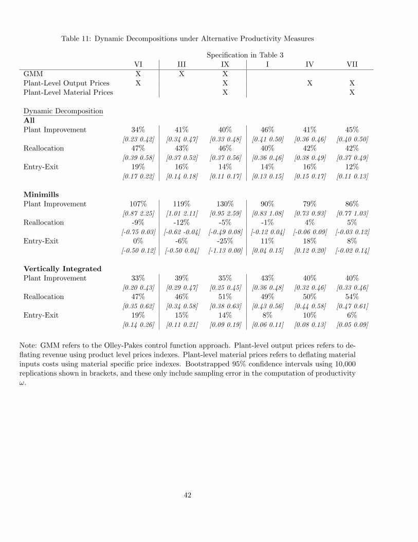
Table 11: Dynamic Decompositions under Alternative Productivity Measures

Specification in Table 3VI III IX I IV VII

GMM X X XPlant-Level Output Prices X X X XPlant-Level Material Prices X X

Dynamic Decomposition

AllPlant Improvement 34% 41% 40% 46% 41% 45%

[0.23 0.42] [0.34 0.47] [0.33 0.48] [0.41 0.50] [0.36 0.46] [0.40 0.50]

Reallocation 47% 43% 46% 40% 42% 42%[0.39 0.58] [0.37 0.52] [0.37 0.56] [0.36 0.46] [0.38 0.49] [0.37 0.49]

Entry-Exit 19% 16% 14% 14% 16% 12%[0.17 0.22] [0.14 0.18] [0.11 0.17] [0.13 0.15] [0.15 0.17] [0.11 0.13]

MinimillsPlant Improvement 107% 119% 130% 90% 79% 86%

[0.87 2.25] [1.01 2.11] [0.95 2.59] [0.83 1.08] [0.73 0.93] [0.77 1.03]

Reallocation -9% -12% -5% -1% 4% 5%[-0.75 0.03] [-0.62 -0.04] [-0.49 0.08] [-0.12 0.04] [-0.06 0.09] [-0.03 0.12]

Entry-Exit 0% -6% -25% 11% 18% 8%[-0.50 0.12] [-0.50 0.04] [-1.13 0.00] [0.04 0.15] [0.12 0.20] [-0.02 0.14]

Vertically IntegratedPlant Improvement 33% 39% 35% 43% 40% 40%

[0.20 0.43] [0.29 0.47] [0.25 0.45] [0.36 0.48] [0.32 0.46] [0.33 0.46]

Reallocation 47% 46% 51% 49% 50% 54%[0.35 0.62] [0.34 0.58] [0.38 0.63] [0.43 0.56] [0.44 0.58] [0.47 0.61]

Entry-Exit 19% 15% 14% 8% 10% 6%[0.14 0.26] [0.11 0.21] [0.09 0.19] [0.06 0.11] [0.08 0.13] [0.05 0.09]

Note: GMM refers to the Olley-Pakes control function approach. Plant-level output prices refers to de-flating revenue using product level prices indexes. Plant-level material prices refers to deflating materialinputs costs using material specific price indexes. Bootstrapped 95% confidence intervals using 10,000replications shown in brackets, and these only include sampling error in the computation of productivityω.

42

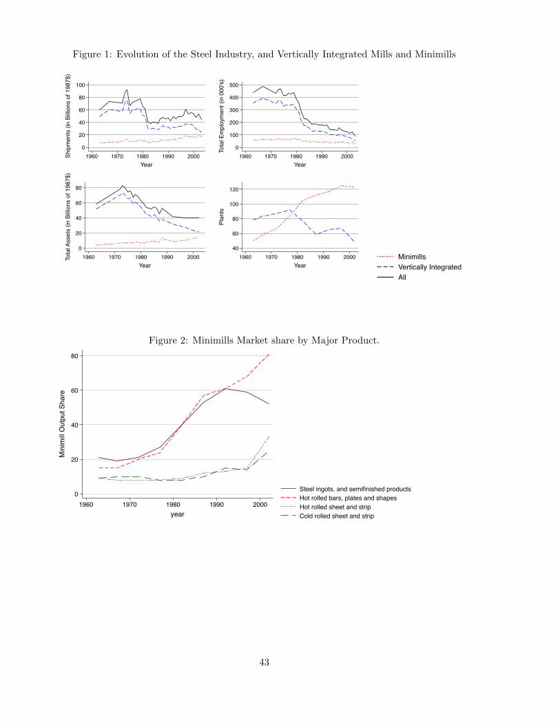
Figure 1: Evolution of the Steel Industry, and Vertically Integrated Mills and Minimills

0

20

40

60

80

100

Ship

men

ts (i

n Bi

llions

of 1

987$

)

1960 1970 1980 1990 2000Year

0

100

200

300

400

500

Tota

l Em

ploy

men

t (in

000

's)

1960 1970 1980 1990 2000Year

0

20

40

60

80

Tota

l Ass

ets

(in B

illion

s of

198

7$)

1960 1970 1980 1990 2000Year

40

60

80

100

120

Plan

ts

1960 1970 1980 1990 2000Year

0

20

40

60

80

100

Ship

men

ts (i

n Bi

llions

of 1

987$

)

1960 1970 1980 1990 2000Year

MinimillsVertically IntegratedAll

Figure 2: Minimills Market share by Major Product.

0

20

40

60

80

Min

imill

Out

put S

hare

1960 1970 1980 1990 2000year

ingotsHRBHRSCRS

0

20

40

60

80

Min

imill

Out

put S

hare

1960 1970 1980 1990 2000year

Steel ingots, and semifinished productsHot rolled bars, plates and shapesHot rolled sheet and stripCold rolled sheet and strip

43

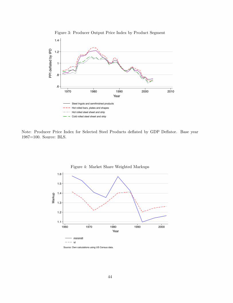
Figure 3: Producer Output Price Index by Product Segment

.6

.8

1

1.2

1.4

PPI d

eflat

ed b

y IP

D

1970 1980 1990 2000 2010Year

Steel Ingots and semifinished productsHot rolled bars, plates and shapesHot rolled steel sheet and stripCold rolled steel sheet and strip

Note: Producer Price Index for Selected Steel Products deflated by GDP Deflator. Base year1987=100. Source: BLS.

Figure 4: Market Share Weighted Markups

1.1

1.2

1.3

1.4

1.5

1.6

Mar

kup

1960 1970 1980 1990 2000Year

minimillvi

Source: Own calculations using US Census data.

44

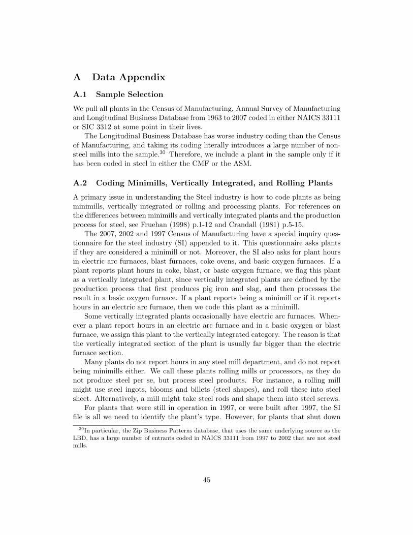
A Data Appendix

A.1 Sample Selection

We pull all plants in the Census of Manufacturing, Annual Survey of Manufacturingand Longitudinal Business Database from 1963 to 2007 coded in either NAICS 33111or SIC 3312 at some point in their lives.

The Longitudinal Business Database has worse industry coding than the Censusof Manufacturing, and taking its coding literally introduces a large number of non-steel mills into the sample.30 Therefore, we include a plant in the sample only if ithas been coded in steel in either the CMF or the ASM.

A.2 Coding Minimills, Vertically Integrated, and Rolling Plants

A primary issue in understanding the Steel industry is how to code plants as beingminimills, vertically integrated or rolling and processing plants. For references onthe differences between minimills and vertically integrated plants and the productionprocess for steel, see Fruehan (1998) p.1-12 and Crandall (1981) p.5-15.

The 2007, 2002 and 1997 Census of Manufacturing have a special inquiry ques-tionnaire for the steel industry (SI) appended to it. This questionnaire asks plantsif they are considered a minimill or not. Moreover, the SI also asks for plant hoursin electric arc furnaces, blast furnaces, coke ovens, and basic oxygen furnaces. If aplant reports plant hours in coke, blast, or basic oxygen furnace, we flag this plantas a vertically integrated plant, since vertically integrated plants are defined by theproduction process that first produces pig iron and slag, and then processes theresult in a basic oxygen furnace. If a plant reports being a minimill or if it reportshours in an electric arc furnace, then we code this plant as a minimill.

Some vertically integrated plants occasionally have electric arc furnaces. When-ever a plant report hours in an electric arc furnace and in a basic oxygen or blastfurnace, we assign this plant to the vertically integrated category. The reason is thatthe vertically integrated section of the plant is usually far bigger than the electricfurnace section.

Many plants do not report hours in any steel mill department, and do not reportbeing minimills either. We call these plants rolling mills or processors, as they donot produce steel per se, but process steel products. For instance, a rolling millmight use steel ingots, blooms and billets (steel shapes), and roll these into steelsheet. Alternatively, a mill might take steel rods and shape them into steel screws.

For plants that were still in operation in 1997, or were built after 1997, the SIfile is all we need to identify the plant’s type. However, for plants that shut down

30In particular, the Zip Business Patterns database, that uses the same underlying source as theLBD, has a large number of entrants coded in NAICS 33111 from 1997 to 2002 that are not steelmills.

45

pre-1997, we use the material and product trailer to the Census of Manufacturingto classify them.

Minimills can be identified by their input use. Electric arc furnaces use a com-bination of scrap steel and direct-reduced iron as inputs. Thus, if a plant usesany direct-reduced iron, we flag this plant as a minimill. Likewise, if scrap steelrepresents more than 20 percent of a plant’s material use, we flag this plant as aminimill.31

Vertically integrated plants can also be identified from their input use. If a plantuses “Coal for Coke”, this is a good indication that a plant has a blast furnace. Weflag rolling mills by their use of “Steel Shapes and Forms” – steel ingots and so onthat are shaped into steel products.

We also use the product trailer to categorize plants. If a plant produces “CokeOven or Blast Furnace Products”, we flag this plant as vertically integrated. Inaddition, if a plant produces “Cold Rolled Sheet Steel” before 1980, we flag thisplant as vertically integrated, as minimills only started producing cold rolled sheetsin the mid-80s. For references on the changing ability of minimills to produce sheetproducts, see Rogers (2009) on page 162 and chapter 8 of Hall (1997).

Plants are not always consistently coded as either minimills, vertically integrated,or rolling mills from one year to another. Thus, we classify a plant based on itshistory of such flags. Specifically, a plant is vertically integrated if it is flagged assuch at least 80 percent of the time. Likewise, a plant is assigned to the minimillcategory if it is flagged as such at least 80 percent of the time.

Since vertically integrated plants, as their name suggests, are typically engagedin multiple activities, such as having an electric arc furnace and a basic oxygenfurnace, along with a rolling mill, we first flag plants as vertically integrated ornot, then flag the remaining plants as minimills. Leftover plants are assigned to berolling mills.

A.3 Coding Products

We use the product trailer of the Census Bureau to investigate the products pro-duced by steel producers. We categorize products into the following types whichare responsible for 93 percent of output not categorized as “other” or “unclassified”in 1997: Hot-Rolled Steel Bar: SIC 33124, NAICS 3311117; Hot Rolled Sheet andStrip: SIC 33123, NAICS 3311115; Cold Rolled Sheet and Strip: SIC 33127, SIC33167, NAICS 3312211, NAICS 3312211D; Cold Finished Bars and Bar Shapes:SIC 33128, SIC 33168, NAICS 3312213, NAICS 331111F; Steel Ingots and Semi-Finished Shapes: SIC 33122, NAICS 3311113; Steel Wire: SIC 33125, SIC 33155,NAICS 3312225, NAICS 3311119; Steel Pipe and Tube: SIC 33170, SIC 33177,NAICS 3312100, NAICS 331111B.

31Basic oxygen furnaces at vertically integrated plants also can a take a small percent of scrapsteel. For this reason, we flag a plant as a minimill only if scrap steel is a large part of their inputs.

46

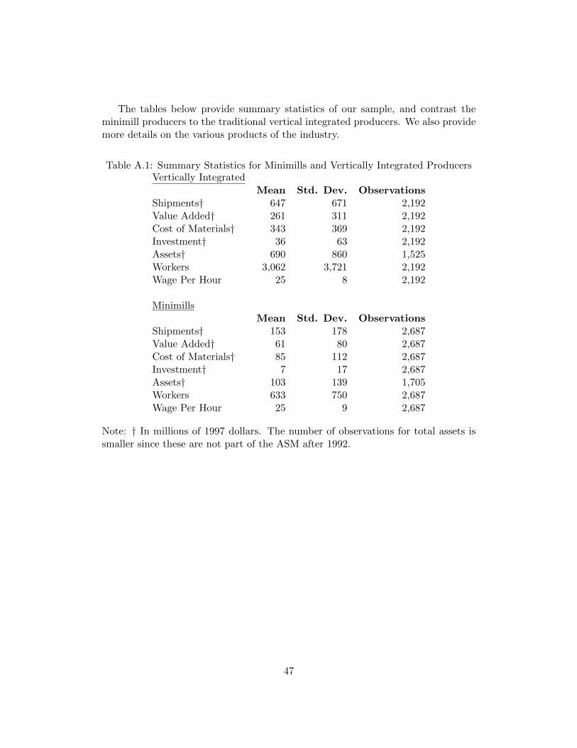
The tables below provide summary statistics of our sample, and contrast theminimill producers to the traditional vertical integrated producers. We also providemore details on the various products of the industry.

Table A.1: Summary Statistics for Minimills and Vertically Integrated ProducersVertically Integrated

Mean Std. Dev. ObservationsShipments† 647 671 2,192Value Added† 261 311 2,192Cost of Materials† 343 369 2,192Investment† 36 63 2,192Assets† 690 860 1,525Workers 3,062 3,721 2,192Wage Per Hour 25 8 2,192

MinimillsMean Std. Dev. Observations

Shipments† 153 178 2,687Value Added† 61 80 2,687Cost of Materials† 85 112 2,687Investment† 7 17 2,687Assets† 103 139 1,705Workers 633 750 2,687Wage Per Hour 25 9 2,687

Note: † In millions of 1997 dollars. The number of observations for total assets issmaller since these are not part of the ASM after 1992.

47

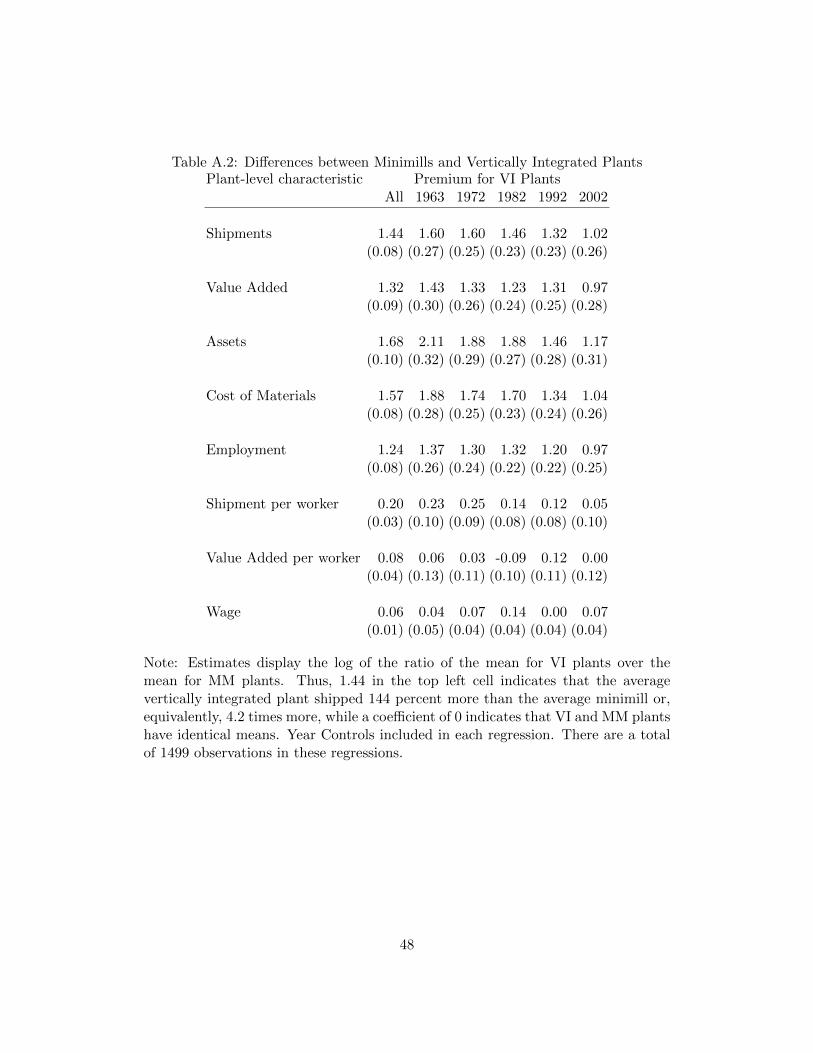
Table A.2: Differences between Minimills and Vertically Integrated PlantsPlant-level characteristic Premium for VI Plants

All 1963 1972 1982 1992 2002

Shipments 1.44 1.60 1.60 1.46 1.32 1.02(0.08) (0.27) (0.25) (0.23) (0.23) (0.26)

Value Added 1.32 1.43 1.33 1.23 1.31 0.97(0.09) (0.30) (0.26) (0.24) (0.25) (0.28)

Assets 1.68 2.11 1.88 1.88 1.46 1.17(0.10) (0.32) (0.29) (0.27) (0.28) (0.31)

Cost of Materials 1.57 1.88 1.74 1.70 1.34 1.04(0.08) (0.28) (0.25) (0.23) (0.24) (0.26)

Employment 1.24 1.37 1.30 1.32 1.20 0.97(0.08) (0.26) (0.24) (0.22) (0.22) (0.25)

Shipment per worker 0.20 0.23 0.25 0.14 0.12 0.05(0.03) (0.10) (0.09) (0.08) (0.08) (0.10)

Value Added per worker 0.08 0.06 0.03 -0.09 0.12 0.00(0.04) (0.13) (0.11) (0.10) (0.11) (0.12)

Wage 0.06 0.04 0.07 0.14 0.00 0.07(0.01) (0.05) (0.04) (0.04) (0.04) (0.04)

Note: Estimates display the log of the ratio of the mean for VI plants over themean for MM plants. Thus, 1.44 in the top left cell indicates that the averagevertically integrated plant shipped 144 percent more than the average minimill or,equivalently, 4.2 times more, while a coefficient of 0 indicates that VI and MM plantshave identical means. Year Controls included in each regression. There are a totalof 1499 observations in these regressions.

48

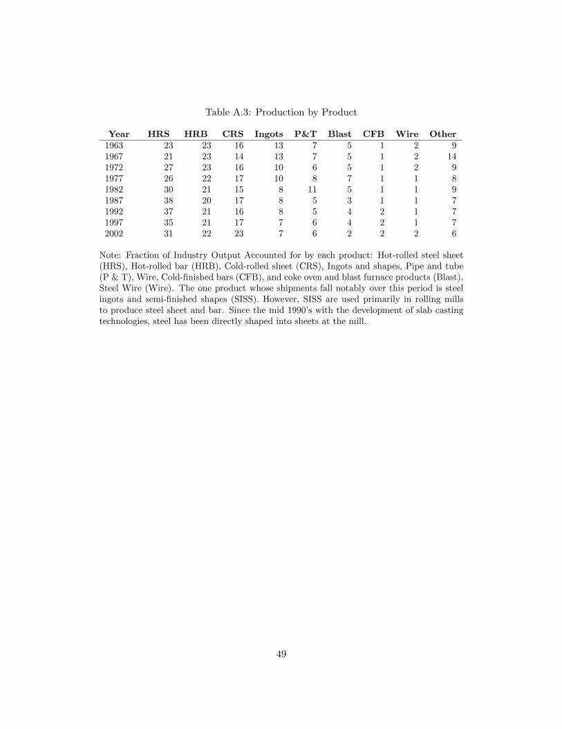
Table A.3: Production by Product

Year HRS HRB CRS Ingots P&T Blast CFB Wire Other1963 23 23 16 13 7 5 1 2 91967 21 23 14 13 7 5 1 2 141972 27 23 16 10 6 5 1 2 91977 26 22 17 10 8 7 1 1 81982 30 21 15 8 11 5 1 1 91987 38 20 17 8 5 3 1 1 71992 37 21 16 8 5 4 2 1 71997 35 21 17 7 6 4 2 1 72002 31 22 23 7 6 2 2 2 6

Note: Fraction of Industry Output Accounted for by each product: Hot-rolled steel sheet(HRS), Hot-rolled bar (HRB), Cold-rolled sheet (CRS), Ingots and shapes, Pipe and tube(P & T), Wire, Cold-finished bars (CFB), and coke oven and blast furnace products (Blast),Steel Wire (Wire). The one product whose shipments fall notably over this period is steelingots and semi-finished shapes (SISS). However, SISS are used primarily in rolling millsto produce steel sheet and bar. Since the mid 1990’s with the development of slab castingtechnologies, steel has been directly shaped into sheets at the mill.

49

B Output and Input Deflators

Recovering productivity using revenue and expenditure data requires that we correctfor potential price variation across plants and time, for both output and inputs.Below, we describe our procedure.

B.1 Output price deflator

In order to guarantee that we recover productivity, ωit, using plant/product revenuedata we rely on a plant-specific output deflator. We construct this deflator usingproduct-level revenues at the plant level (recorded in the census data) in combinationwith product-level price data (from the BLS).32

To make sure that price variation – across plants and time – is fully controlledfor, we assume the following structure: Plants charge the same markup across alltheir products, while markups can flexibly vary across plants and time. The hetero-geneity in markups will naturally arise if plants are heterogeneous in their underlyingproductivity.

Before we derive the exact price deflator, we state explicitly what we observe inthe data: revenues (Rijt), input (Xit) and prices (Pjt).

We start out with the following production function:

Qijt = XijtΩit, (B.1)

where we are explicit about productivity only being plant-specific and not plant-product-specific. The input bundle Xijt contains labor, intermediate inputs andcapital, scaled by their corresponding technology parameters, X = LβlKβkMβm .

Now consider plant-level revenue, which is obtained by summing product-specificrevenues, and using the production function:

Rit =∑j

XijtΩitPjt. (B.2)

To recover plant-level productivity from a regression of plant-level (deflated)revenues and input use, we use:

Xijt ≡ sijtXit (B.3)

Plugging the last expression into the one for plant-level revenue, we get:

32Specifically, we use the following BLS price series: PCU331111331111: Steel;PCU3311113311111: Coke oven and blast furnace products; PCU3311113311113: Steel in-gots and semifinished products; PCU3311113311115: Hot rolled steel sheet and strip;PCU3311113311117: Hot rolled steel bars, plates, and structural shapes; PCU3311113311119: Steelwire; PCU331111331111B: Steel pipe and tube; PCU331111331111D: Cold rolled steel sheet andstrip and PCU331111331111F: Cold finished steel bars.

50

Rit = ΩitXit

∑j

sijtPjt (B.4)

Up to sijt, which we will discuss below, everything is directly observable and,therefore, we can recover productivity using standard estimation techniques using:

Rit∑j sijtPjt

= XitΩit (B.5)

or in logs:

rit − pit = βllit + βkkit + βmmit + ωit + εit, (B.6)

where pit ≡∑

j sijtPjt is the plant-level output price deflator, and we use that the(log) input bundle can be decomposed into labor and capital input, scaled by theircorresponding output elasticity β. The additional error term εit captures measure-ment error in either revenue or prices, as well as unanticipated shocks to output.

In order to take equation (B.6) to the data, we need to take a stand on the inputallocation or what sijt is. We use revenue shares:

sijt =Rijt∑j Rijt

, (B.7)

which we can directly compute in our data. The use of revenue shares restricts themarkups to be the same across the products of a, potentially, multi-product plant.To see this it is useful to use the framework of De Loecker and Warzynski (2012) torecover markups and apply it to our setting. The markup µijt is obtained using theFOC on input X of cost minimization:

µijt = βXRijt

PXit sijtXit. (B.8)

Now, using equation (B.7), we get the following expression for markups:

µijt = βXRit

PXit Xit(B.9)

which highlights that µijt = µit and ∀j ∈ Ji, with Ji the set of products producedby i.

Note that the reason we need to restrict markups across products within a plantto be constant, is because we see aggregate input use only at the plant level.33

Finally, although we directly observe revenues for all product-plant combinations,we only observe product specific prices and assume away the variation across plants

33See De Loecker and Warzynski (2012) and De Loecker, Goldberg, Khandelwal, and Pavcnik(2012) for a detailed discussion of the input allocation across products.

51

for a given product. In our empirical analysis, we rely on both the aggregate priceindex and our constructed plant-specific price index.

B.2 Input price deflator

The construction of the input price deflator is very similar to that of the outputprice deflator. There are, however, a few important differences. First, we need todistinguish between our three main input categories: labor, intermediate inputs andcapital. Second, for some of the inputs, we observe plant-level input prices, that wecan directly use to construct the deflator.

B.2.1 Labor and capital

We directly observe hours worked at the plant-level. We rely on the NBER capitaldeflator to correct the capital stock series. The use of an aggregate deflator impliesthat we assume a common user cost of capital across plants.

B.2.2 Intermediate inputs

The data on intermediate input use is potentially the most contaminated by inputprice variation, both in the cross-section and in the time series and, in particular,across the two types: VI and MM. As discussed in the main text, both technologiesuse vastly different intermediate inputs or use inputs at very different intensities.Note that the share of all intermediate inputs is not significantly different acrosstypes, but this masks the underlying heterogeneity. Due to the very different inputuse, we are concerned that the aggregate deflator does not fully capture the inputprice differences across plants and time.

We construct a plant-level intermediate input price deflator in the followingway. We consider n intermediate inputs where n=Fuel (F), Electricity (E), Coalfor coke (C), iron ore (I), iron and scrap (S), Others (O). In the data we observeexpenditures by intermediate input (ME

int) and prices for each input n (Pnit).The plant-level intermediate input price deflator is constructed as follows:

PMit =∑n

snitPnt (B.10)

snit =MEint∑

nMEit

(B.11)

Pnt = N−1∑i

Pnit . (B.12)

In words, we compute the average price for a given input n, Pnt , and weigh thisby the plant’s input share snit. This structure still assumes a common input pricefor all plants for a given input n, but it recognizes that the intensity can vary across

52

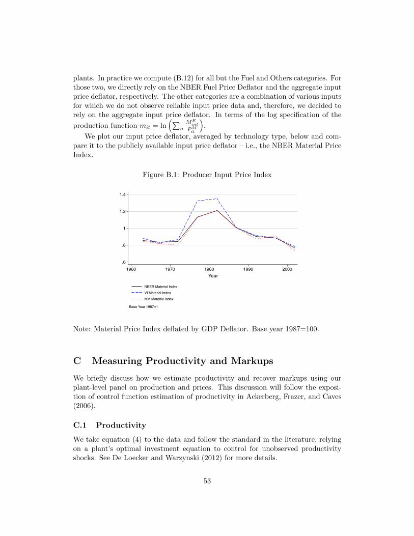
plants. In practice we compute (B.12) for all but the Fuel and Others categories. Forthose two, we directly rely on the NBER Fuel Price Deflator and the aggregate inputprice deflator, respectively. The other categories are a combination of various inputsfor which we do not observe reliable input price data and, therefore, we decided torely on the aggregate input price deflator. In terms of the log specification of the

production function mit = ln(∑

nMEint

PMit

).

We plot our input price deflator, averaged by technology type, below and com-pare it to the publicly available input price deflator – i.e., the NBER Material PriceIndex.

Figure B.1: Producer Input Price Index

.6

.8

1

1.2

1.4

1960 1970 1980 1990 2000Year

NBER Material IndexVI Material IndexMM Material Index

Base Year 1987=1

Note: Material Price Index deflated by GDP Deflator. Base year 1987=100.

C Measuring Productivity and Markups

We briefly discuss how we estimate productivity and recover markups using ourplant-level panel on production and prices. This discussion will follow the exposi-tion of control function estimation of productivity in Ackerberg, Frazer, and Caves(2006).

C.1 Productivity

We take equation (4) to the data and follow the standard in the literature, relyingon a plant’s optimal investment equation to control for unobserved productivityshocks. See De Loecker and Warzynski (2012) for more details.

53

Specifically, the first stage of this procedure runs output qit on a flexible functionof inputs (lit,mit, kit), an investment control function iit, as well as year-plant typecontrols. In other words:

qit = φψ,t(lit,mit, kit, iit) + εit. (C.1)

And productivity is recovered as ωit = φit− fψ,t(Lit,Mit,Kit;β). A key compo-nent in the estimation routine is the law of motion on productivity. In our baselineresults, we stick to an exogenous Markov process given by

ωit = gψ(ωit−1, χit) + ξit. (C.2)

Note that this evolution is allowed to vary for minimills and vertically integratedplants, as we have seen in the OLS regressions that vertically integrated plantsslowly catch up to minimills. Moreover, we control for the selection effect due tothe fact that we only observed productivity conditionally on a plant remaining inthe industry using the estimated propensity score of exiting χit. To the extent thatvertically integrated plants are larger and thus, at an ex-ante level more likely toremain in the industry, this will generate differential selection rules for minimillsand vertically integrated plants.

We recover estimates of the production function coefficients, β, by forming mo-ments on this productivity shock ξit. The identification of these coefficients relies onthe rate at which inputs adjust to these shocks. In particular, we allow both laborand capital to be dynamically chosen inputs, whereby current values of capital (la-bor) do not react to current shocks to productivity (ξit). Plants do, however, adjusttheir intermediate input use (scrap, energy, other material inputs) to the arrival ofa productivity shock ξit.

The exact moments will depend on the functional form we select for f(.). Forour main specifications, we rely on Cobb-Douglas production functions and use thefollowing moments:

E

ξit(β)

litmit−1

kit

= 0. (C.3)

A recent literature (Ackerberg, Frazer, and Caves, 2006) has pointed out thatthe identification of the variable input, the coefficient of βm in our case, relies onsufficient variation in plant-level input prices. The coefficient on labor (capital)is identified using variation in adjustment cost and relies on the fact that plantscannot immediately adjust their labor (capital) use to a productivity shock. Allour results are invariant to modifications of the timing assumptions discussed inthe main text. Our approach is flexible and can allow for a variety of productionfunctions combined with various assumptions on the variability of inputs, as well asthe use of alternative proxies such as intermediate inputs.

54

C.2 Estimating Markups

Our approach to recovering markups follows De Loecker and Warzynski (2012). Inthe rest of this section, we briefly review the approach. In addition to the productionfunction we introduced before, we only have to assume that producers active in themarket minimize costs. Let Vit denote the vector of variable inputs used by thefirm. We use the vector Kit to denote dynamic inputs of production. Any inputthat faces adjustment costs will fall into this category; capital is an obvious one,but our framework allows us to also include labor.

The associated Lagrangian function is:

L(V 1it , ..., V

Vit ,Kit, λit) =

V∑v=1

Pv

itVvit + ritKit + λit(Qit −Qit(V 1

it , ..., VVit ,Kit, ωit))

(C.4)where P

v

it and rit denote a firm’s input prices for a variable input v and dynamic in-puts, respectively. The first-order condition for any variable input free of adjustmentcosts is

∂Lft∂V v

it

= Pv

it − λit∂Qit(.)

∂V vit

= 0. (C.5)

where the marginal cost of production at a given level of output is λit, as ∂Lit∂Qit

=

λit. Rearranging terms and multiplying both sides by VitQit

, generates the followingexpression.

∂Qit(.)

∂V vit

V vit

Qit=

1

λit

P vitVvit

Qit(C.6)

Cost minimization implies that optimal input demand is realized when a firmequalizes the output elasticity of any variable input V v

it to 1λit

P vitVitQit

.

Define markup µit as µit ≡ Pitλit

. As De Loecker and Warzynski (2012) show, thecost-minimization condition can be rearranged to write markup as:

µit = θvit(αvit)−1. (C.7)

where θvit denotes the output elasticity on an input V v and αvit is the revenue share

of variable input v, defined byP vitV

vit

PitQit, which is data. This expression will form the

basis for our approach: We obtain the output elasticity from the estimation of aproduction function and only need to measure the share of an input’s expenditurein total sales. In particular, in our setting, θvit = βm.

In our context, the output elasticities are obtained by relying on product-specificprice deflators, and potentially leave plant-level price variation left uncontrolledfor. The latter is expected to bias the output elasticity downward and, therefore,downward-bias the level of the markup. Under a Cobb-Douglas production tech-nology, this has no implications for the time-series pattern of markups and on thecomparison of markups across minimills and integrated producers – as long as the

55

output elasticity is fixed across types.

D Deriving decompositions

We provide more details on how we derive the various decompositions introducedin the main text. We start with the standard aggregate productivity definition:

Ωt =∑i

sitωit (D.1)

where we define:

sit =Rit∑iRit

(D.2)

Rt =∑i

Rit (D.3)

and Rit is plant-level total sales.

D.1 Standard OP

Olley and Pakes show that (D.1) can be written as:

Ωit = ωt +∑i

(sit − st)(ωit − ωt)

= ωt + ΓOPt

(D.4)

with Nt the number of active plants at time t and:

ωt = N−1∑i

ωit (D.5)

st = N−1∑i

sit (D.6)

D.2 Deriving the Between covariance

We show that aggregate productivity can be decomposed in a between technologycovariance component and an average type-specific productivity component, whichin itself is decomposed into type-specific within and covariance terms.

Start from (D.1) and simply break up the sum into the two technology types,i.e. ψ = MM,V I:

56

Ωt =∑

i∈ψ=MM

sitωit +∑

i∈ψ=V I

sitωit

= st(ψ = MM)∑

i∈ψ=MM

sitst(ψ = MM)

ωit

+ st(ψ = V I)∑

i∈ψ=V I

sitst(ψ = V I)

ωit

(D.7)

The second line multiplies and divides each term by the relevant total marketshare of the type in the industry, i.e. st(ψ) =

∑i∈ψ sit.

34

The last equation can now be rewritten as another weighted sum where we nowsum over two groups: minimills and intergrated producers:

Ωt =∑ψ

st(ψ)Ωt(ψ) (D.8)

where

Ωt(ψ) =∑i∈ψ

sitst(ψ)

ωit =∑i∈ψ)

sit(ψ)ωit (D.9)

The second line uses that the market share of a plant in the total industry dividedby the total type-specific market share is equal to the plant’s market share in thetype’s total sales (sit(ψ)). Formally:

sit(ψ) =sitst(ψ)

(D.10)

After having transformed the aggregate productivity expression into (D.8), wecan rely on the same insight as OP and decompose aggregate productivity into aunweighted average and a covariance component. By transforming the expressionusing type-specific market shares we guarantee that the plant market shares sum toone; a necessary condition for the OP decomposition.

Applying the OP decomposition idea to (D.8) gives us:

Ωt = Ωt(ψ) +∑ψ

(st(ψ)− 0.5)(Ωt(ψ)− Ωt(ψ))

= Ωt(ψ) + ΓBt

(D.11)

34The OP-decomposition relies crucially on the property that the market shares sum to one.However, if we were to simply split the summation across the two types, we could not isolate thewithin covariance term. To see this, note that

∑ψ Ωt(ψ) 6= Ωt, due to the fact that

∑ψ,i sit(ψ) > 1.

57

D.3 Within type decompositions

Starting from equation (D.11) we simply apply the OP decomposition by type ψand use the fact that we only have two technology types to obtain an expression forthe average component:

Ωt(ψ) =1

2

∑ψ

(Ωt(ψ))

=1

2

∑ψ

(ωt(ψ) +∑i∈ψ

(sit(ψ)− st(ψ))(ωit − ωt(ψ)))

=1

2

∑ψ

(ωt(ψ) + ΓOPt (ψ))

(D.12)

where we denote the average market share across a given type by st(ψ) =N−1ψ

∑i∈ψ sit(ψ).

D.4 Total decomposition

To arrive at the expressions used in the main text we introduce Γt(ψ) to denote acovariance of a given type and use superscripts B and OP to indicate whether thecovariance is between or within the type, respectively. This gives us the followingtotal decomposition of aggregate productivity:

Ωt =1

2

∑ψ

[ωt(ψ) + ΓOPt (ψ)] + ΓBt (ψ) (D.13)

If there was no entry or exit we can then directly evaluate the share of eachcomponent by tracking Ωt over time. We incorporate the turnover process by relyingon dynamic decompositions within a given type and can always scale the varioussubcomponents back to the decomposition discussed above.

58