Realization of a motility-trap for active particles

ARTICLE

Realization of a motility-trap for active particlesSoudeh Jahanshahi1, Celia Lozano 2, Benno Liebchen3, Hartmut Löwen1 & Clemens Bechinger 2✉

Trapping of atomic and mesoscopic particles with optical fields is a practical technique

employed in many research disciplines. Developing similar trapping methods for self-pro-

pelled, i.e. active, particles is, however, challenging due to the typical anisotropic material

composition of Janus-type active particles. This renders their trapping with magneto-optical

fields to be difficult. Here we present the realization of a motility-trap for active particles,

which only exploits their self-propulsion properties. By combining experiments, numerical

simulations, and theory, we show that, under appropriate conditions, a force-free rotation of

the self-propulsion direction towards the trap's center can be achieved, which results in an

exponential localization of active particles. Because this trapping mechanism can be applied

to any propulsion scheme, we expect such motility-tweezers to be relevant for fundamental

studies of self-driven objects as well as for their applications as autonomous microrobots.

https://doi.org/10.1038/s42005-020-0393-4 OPEN

1 Institut für Theoretische Physik II: Weiche Materie, Heinrich-Heine-Universität Düsseldorf, 40225 Düsseldorf, Germany. 2 Fachbereich Physik, UniversitätKonstanz, 78457 Konstanz, Germany. 3 Institut für Festkörperphysik Technische, Universität Darmstadt, 64289 Darmstadt, Germany. ✉email: [email protected]

COMMUNICATIONS PHYSICS | (2020) 3:127 | https://doi.org/10.1038/s42005-020-0393-4 | www.nature.com/commsphys 1

1234

5678

90():,;

Konstanzer Online-Publikations-System (KOPS) URL: http://nbn-resolving.de/urn:nbn:de:bsz:352-2-13ecjwgy7kft30

http://crossmark.crossref.org/dialog/?doi=10.1038/s42005-020-0393-4&domain=pdf




http://orcid.org/0000-0001-5830-1154

http://orcid.org/0000-0001-5830-1154

http://orcid.org/0000-0001-5830-1154

http://orcid.org/0000-0001-5830-1154

http://orcid.org/0000-0001-5830-1154

http://orcid.org/0000-0002-5496-5268

http://orcid.org/0000-0002-5496-5268

http://orcid.org/0000-0002-5496-5268

http://orcid.org/0000-0002-5496-5268

http://orcid.org/0000-0002-5496-5268

mailto:[email protected]

mailto:[email protected]

www.nature.com/commsphys


The development of techniques aiming to spatially position,confine, or trap particles in space has promoted some ofthe most spectacular advancements in fundamental and

applied science throughout the past few decades. On atomicscales, such trapping techniques have led, for example, to therealization of Bose–Einstein condensates1–3, and play an impor-tant role in the development of quantum computers4,5 based ontrapped ions. On the micron- and nanoscale, the invention ofoptical tweezers6,7 enables to exert well-controlled forces onviruses, living cells, and synthetic colloids to probe, for example,the viscoelastic properties of DNA and cell membranes, or tomeasure forces exerted by molecular motors7,8.

An important class of particles for which effective and versatiletrapping schemes are currently not available are self-propelled activeparticles (APs)9–15. Such systems receive considerable attention dueto their resemblance with motile microorganisms16–18, allowing toidentify general conditions under which collective behavior canemerge19,20. In addition, APs are currently discussed as autonomousmicrorobots that may find use as autonomous vehicles to deliverloads to specific targets21–23. In view of such applications, there isgrowing need to finely control their location in space and time,which, for example, allows to maintain high densities of APs atspecific positions. Compared to Brownian particles, the application ofoptical traps is not straightforward, partly because APs are typicallycomposed of nonuniform dielectric materials, including partialmetallic coatings, which lead to non-isotropic optical forces andstrong light scattering effects. Accordingly, present trappingmechanisms of APs require the presence of pores and walls24–31,external forces22,23,32–39, or the presence of other particles40,41.

Here, we present a novel trapping mechanism of APs, whichsolely originates from their self-propulsion and does not requireexternal forces. To demonstrate such motility trapping, we per-form experiments with APs whose self-propulsion is controlledby light. We want to emphasize, however, that our results can bealso applied to APs propelled by, for example, self-diffusiophoresis14,42 or self-thermophoresis15. Using experi-ments, simulations, and analytical theory, we show that a non-monotonic spatial variation of the particle’s motility (exhibitingeither a maximum or a minimum) leads to the localization ofAPs, which are unbound otherwise. To characterize this locali-zation in detail, we introduce a trapping classification scheme bydefining general criteria for “strong” and “weak” particle locali-zation. In contrast to most other trapping mechanisms, which areless effective at high propulsion velocities, the motility trap pre-sented here is particularly efficient for fast APs. In addition topractical implications, the presented motility traps can be alsoused to determine coupling coefficients of APs to external fields.

ResultsOutline of the experimental approach. APs are made fromcolloidal silica particles with a diameter σ= 3.25 μm, which arehalf-coated with a 50-nm carbon layer on one hemisphere andafterwards suspended in a critical mixture of water and 2,6-luti-dine (lutidine mass fraction 0.286). The temperature of the entiresample cell is kept constant several degrees below its lower criticalpoint Tc= 34.1 °C43,44. Due to gravity, the particles are confinedto the bottom of the sample cell where they perform a two-dimensional motion. Under laser illumination (λ= 532 nm), lightis mainly absorbed at the carbon cap, leading to the preferentialheating of the cap. Once the cap temperature exceeds, Tc, thisresults in a local demixing of the adjacent fluid. In our experi-ments, such conditions are achieved above a threshold intensityof I0 ~ 0.08 μW μm−2. Depending on the light intensity, thedemixing region is characterized by a single or (at higher inten-sities) two single-phase droplet(s) that nucleate around the

particle. The droplet’s asymmetrical shape leads to a propulsivevelocity v, which depends on the light intensity in a strongly non-monotonic fashion (Fig. 1a)43,45. While v linearly increases atsufficiently low intensities, it sharply reverses its direction nrelative to the cap above a certain intensity threshold Ir ~ 0.58μW μm−2 when a second droplet covers the uncapped surface(see Fig. 1a and “Methods” for details). Due to the additionalpresence of rotational diffusion (Dr ~ 1/50 s), the APs perform anunbiased persistent random motion under homogeneous illumi-nation conditions.

In the presence of a light gradient ∇I, the shape of thenucleating droplets around the APs is no longer symmetricrelative to n. As a consequence, AP motion becomes stronglybiased leading to a phototactic behavior43. Depending on whetherthe illumination intensity is below or above Ir, APs will

Fig. 1 Light-activated motion. a Measured propulsion velocity v of theactive particle (AP) vs. illumination intensity I. Above a threshold intensityI0 ~ 0.08 μW μm−2 the propulsion mechanism sets in, leading to self-propulsion. The vector n corresponds to the direction of propulsion andreverses its sign at the critical intensity Ir. b Example of measuredtrajectories of an AP in a static light gradient ∇I. Below Ir the AP movesopposite to ∇I (negative phototaxis, blue trajectory and background).Above Ir the particle moves along ∇I (positive phototaxis, red trajectory andbackground). Time evolution of the angle ϕ between the propulsiondirection of the AP and the direction of the light gradient, after the AP issuddenly exposed to the light gradient for intensities c below Ir and d aboveIr. Squares denote averaged data, and the full line shows the theoretical fits.In both cases, an identical light gradient of intensity ∇Ij j= 0.1 μW μm−3

was used. Inset: Sketch of an AP in a positive and negative light gradienttogether with the resulting angular velocity ω at which the AP rotates whenthe light gradient is switched on. Error bars denote the standard deviation.

ARTICLE COMMUNICATIONS PHYSICS | https://doi.org/10.1038/s42005-020-0393-4

2 COMMUNICATIONS PHYSICS | (2020) 3:127 | https://doi.org/10.1038/s42005-020-0393-4 | www.nature.com/commsphys


experience an aligning torque leading to their propulsion opposite(negative phototaxis) or along ∇I (positive phototaxis), respec-tively (Fig. 1b). To characterize the particle’s alignment, we havemeasured their reorientation dynamics within a light gradient.Experimentally, this was achieved by suddenly turning on a lightgradient in x-direction when the particle propulsion direction nwas pointing along the positive x-direction (dashed line in theinsets of Fig. 1c). As a result of the droplet’s asymmetry, theparticle will realign until n is antiparallel (negative phototaxis) orparallel (positive phototaxis). This orientation process is shown inFig. 1c, with ϕ being the angle between n and the x-direction (seeinset).

Theoretical model. To describe our experimental findings, weconsider the motion of an overdamped self-propelled particlewhose propulsion velocity v(x) varies in space and which canalign parallel or antiparallel to the local intensity gradientdepending on the tactic condition. This leads to the followingLangevin equations for the center of mass position r(t)= (x(t), y(t)) and the self-propulsion direction n= (cos(ϕ), sin(ϕ))expressed by its angle ϕ with the x-axis (see ref. 46 for details)

_r tð Þ ¼ v xð Þnþffiffiffiffiffiffi2D

pξðtÞ; ð1Þ

_ϕðtÞ ¼ ω ϕ; xð Þ þ ffiffiffiffiffiffiffiffi2Dr

pξϕ: ð2Þ

Here, ξ tð Þ ¼ ξx tð Þ; ξy tð Þ� �

; ξϕ tð Þ describe Gaussian white noise,

with zero mean and unit variance, and D and Dr correspond tothe translational and rotational diffusion coefficients, respectively.

As will be later shown in our experiments, the key mechanismfor the motility trap is the active alignment of APs relative to thelocal intensity gradient. The instantaneous alignment rate ωdepends on both the surface-averaged total velocity of the solventaround the AP and its asymmetry relative to the AP orientation47.Since the magnitude of the surface-averaged flow velocity alsocontrols the self-propulsion speed47, on the one hand, we expectω∝ v. On the other hand, the dependence of ω on the flow fieldasymmetry suggests ω∝ |∇I| or ω / v0 xð Þ ¼ dvðxÞ=dx. This leads

to the following overall expression for the phototactic alignmentrate ω ϕ; xð Þ ¼ c

σ v xð Þv0 xð Þsin ϕ (see ref. 46 regarding the determi-nation of the coefficients). Here, we have introduced the particlediameter σ occurring in the denominator since alignmentcompetes with the rotational drag, the latter linearly scaling withσ. Finally, the coefficient c, a parameter fixed by experiments,determines if phototaxis is positive (c < 0) or negative (c > 0) (see“Methods” for further details). With this form for the alignmentrate, the orientational dynamics, as obtained from the noise-freesolution of (1) and (2), is in good agreement with theexperimental observations, see Fig. 1c, d.

Realization of an AP motility trap. A motility trap requires aposition-dependent AP realignment mechanism, which preventsit from leaving a certain spatial region. In our experiments, this isachieved by a spatial light profile, which is created by periodicallyscanning a line-shaped laser beam with a mirror across thesample plane (see “Methods”). Synchronization of the mirrormotion with an electro-optical intensity modulator yields toillumination of APs with arbitrary one-dimensional illuminationprofiles (Fig. 2a). Since the scanning frequency of the mirror is setto 200 Hz, this leads to quasi-static illumination conditions forthe APs. In our experiments, we created triangular-shapedintensity fields with either an intensity minimum (Fig. 2b) oran intensity maximum (Fig. 2c), each characterized by the widthof lv, which has been varied between 8 and 300 µm. The profile inFig. 2b varies between I= 0.08 and 0.4 µW µm−2, with theintensity minimum located at x= 0. Since the intensities arebelow Ir, under such conditions APs will always align towards theintensity minimum, that is, opposite to ∇I (see Fig. 1b). Con-versely, for the profile shown in Fig. 2c, the intensity variesbetween I= 0.58 and 0.9 µW µm−2, with the maximum at x= 0.Because this intensity range is above Ir, here APs align towardsthe intensity maximum, that is. parallel to ∇I (see Fig. 1b).

We start by a qualitative discussion of the experimental resultsfor the conditions shown in Fig. 2b. In addition to affecting thealignment of APs, a position-dependent light field I(x) leadws to aspatial variation of self-propulsion velocity v(x) shown in Fig. 2d.

Fig. 2 Experimental realization of a motility trap. a Sketch of experimental setup. b Spatial intensity profile of a “cooling trap.” The blue line describes theintensity profile of a one-dimensional triangle-shaped light field with period length lv= 150 µm. The intensities are within the range where the particledisplays negative phototaxis, that is, above the threshold intensity I0, but below the critical intensity Ir. Superposed are subsequent snapshots of a typicalactive particle’s (AP) dynamics in such a trap, where the blue arrow describes the direction of motion of the particle. c Same as in b but for a “heating trap”:the red line describes the intensity profile of the light field, which is in the range of positive phototaxis, that is, above the critical intensity Ir. For a coolingtrap: d shows the x-component of the active particle’s velocity, v(x), for outward motion (empty squares) and inward motion (filled circles); e shows anexample of an AP’s trajectory relative to the trap center (horizontal line at x= 0), and f its positional probability distribution P(x). For a heating trap, thecorresponding (g) inward and outward velocities v(x) (h) AP typical motion relative to the trap center, and i its P(x). Error bars correspond to the standarddeviation.

COMMUNICATIONS PHYSICS | https://doi.org/10.1038/s42005-020-0393-4 ARTICLE




The values of v(x) were obtained from the spatially resolvedanalysis of the particle’s trajectories and agree with the valuesshown in Fig. 1a considering a piecewise linear intensity profile(Fig. 2b). To rule out the possible influence of optical forces actingon the APs, v(x) was independently determined for the inward(towards x= 0) and outward (away from x= 0) particle motion.The data show the identical results, which confirm the absence ofoptical gradient forces in our experiment.

The dynamics of the AP within the intensity profile is shown inFig. 2e. When the particle propels away from the intensityminimum, the light gradient reverses its self-propulsion direction,thus leading to an effective trapping mechanism. Because the APcannot instantaneously change its orientation but with a ratewhich is limited by viscous friction, it significantly overshoots thetrapping center, which causes the oscillations around the trappingcenter seen in Fig. 2e. This spatial confinement is confirmed bythe corresponding particle probability distribution function(PDF) (Fig. 2f). Since the AP becomes localized around theposition where v(x) is smallest, in the remainder we refer to suchconditions as a “cooling trap,” in analogy to cold atomsremaining in the vicinity of the minimum of an optical trap48.

In addition, we also performed similar measurements for thelight field shown in Fig. 2c, which features a maximum in thecenter and where the intensities are above Ir. Then, the APsexhibit a positive phototactic response, that is, its swimmingmotion is biased in the direction of ∇I. As for the cooling trap,the AP’s velocity linearly depends on the local light intensity(Fig. 2g), but with the trajectory now being localized around the

intensity maximum (Fig. 2h), which spatial confinement isconfirmed by its P(x) (Fig. 2i). Since v(x) is largest at theseregions, this explains why the oscillations become significantlyenhanced compared to Fig. 2e. In the following, we refer to suchtrapping conditions as a “heating trap.”

As already discussed, the spatial confinement of APs within amotility trap is governed by their orientational response to thelight gradient. We quantify this in Fig. 3a, b by plotting thecharacteristic alignment time τ, defined as the time needed for arotation of the AP between ϕ= 0.14 and 3 rad, as a function of ∇I(see “Methods” for further details). The alignment timemonotonically decreases with increasing |∇I|. In addition, τdecreases when I increases (apart near Ir where the AP motionbecomes instable) because of the stronger solvent flow near theparticle46. This latter dependence also explains why thereorientation dynamics for the cooling trap is slower than thatof a heating trap (Fig. 2e, h).

To obtain the relationship between the alignment time and thewidths of the particle PDFs within the motility traps, we havevaried the intensity profile width lv, which leads to differentintensity gradients. The resulting PDF for the cooling and theheating trap both show a maximum at the trap center withexponentially decaying tails at both sides. As expected, thelocalization becomes more efficient when the alignment time τbecomes faster, that is, when |∇I| increases (symbols in Fig. 3c, d).The observed shape of the PDF is in stark contrast to an APwithout active alignment where it simply follows an effectiveBoltzmann distribution49.

Fig. 3 Localization of active particles (APs) in a motility trap. The data for a cooling and a heating trap are shown in a, c and b, d, respectively. Symbols andsolid lines show experimental data and numerical simulations, respectively. In each plot, different symbols and the curve of the corresponding color correspond tolight profiles with different laser intensities, characterized by the largest velocity Vmax achieved by active particles within each profile. a, b Alignment time τ of an AP

as a function of the intensity gradient ∇Ij j for different laser intensities. The solid curves show the theoretical fit according to τ ¼ 2~C∇I ln

cosðϕωmaxÞþ1

sinðϕωmaxÞ

� �, where ~C is the

fitting parameter and the total rotation ϕωmax¼ 3 rad. Experimental data are averaged over 10 repetitions for each curve. c, d Corresponding probability distribution

function of the particle’s position (x) rescaled by the particle size (σ) in log-lin and (as inset) lin-lin scale. Error bars correspond to the standard deviation.




As a first test of the validity of our theoretical model, we nowdetermine the PDF of APs in the trap by performing Browniandynamics simulations for an ensemble of particles, initialized inthe vicinity of the trapping center, with random initial conditions.As shown in Fig. 3c, d (solid lines), the resulting distributions arein quantitative agreement with our experiments. For positivephototaxis, we obtain a comparatively high propulsion velocitynear the trap center (“heating”); in contrast, the velocity issmallest near the trapping center for the “cooling” trap. In bothcases, the particle distribution decays exponentially as thedistance from the center decreases (Fig. 3c, d ), which leads toa saturation of the mean-square displacement, see Fig. 4a, b.

To further characterize the properties of the motility trap, wealso perform analytical calculations to determine the steady-stateparticle distribution. For weak noise, this yields the followingapproximate expression for the PDF (see “Methods” forcalculation details):

P xð Þ ’π�1 dB xð Þ

dx

�� ffiffiffiffiffiffiffiffiffiffiffiffiffiffiffiffiffiffiffi1� B2 xð Þp ; B xð Þ ¼ exp � c

σv xð Þ � v 0ð Þð Þ

� �: ð3Þ

Here the B2 term in the denominator of Eq. (3) is mainly relevantnear the trapping center x= 0.

Since B(x) decays faster in x for small particle-size (σ) valuesthan for large ones, it follows from Eq. (3) that the tails of thePDF decay faster in x for small particles. This corresponds to thefact that ω∝ 1/σ in Eq. (2), mirroring the fact that larger APs turnslower in a given gradient than small APs. In addition, Eq. (3)shows that the tails of the PDF decay faster as the slope of thegradient increases. Physically, this is because steep gradients biasthe propulsion direction of APs more efficiently towards thetrapping center than shallow gradients.

Mean-square displacement and dynamical correlations. Tocharacterize the AP dynamics within a motility trap, we nowperform Brownian dynamics simulations of our model (details in“Methods” section) and compare our results with experiments.This leads to a close quantitative agreement without any adjus-table fitting parameters (see Fig. 4).

We first discuss the translational and rotational mean-squaredisplacement (Fig. 4). Notice first that there is a plateau occurring

in the mean-square displacement x tð Þ � xð0Þð Þ2� �, which

represents (permanent) trapping in x direction. That is, we candefine (the square of) a length scale corresponding to theconfinement length by

x2� � ¼ Z dx x2 PðxÞ: ð4Þ

The confinement length decreases as the depth of the trap Vmax

increases.In Fig. 4b, we observe peaks preceding the onset of the plateau.

These peaks correspond to the average time an AP needs for a“roundtrip” in the trap, which we denote with �Tosc. Accordingly,the time between t= 0 and the first maximum ofx tð Þ � xð0Þð Þ2� �

is �Tosc=2.For example, particles that are close to the trapping center at a

given time move ballistically outwards and, afterward, reach theirturning point after a characteristic typical time amountingroughly to �Tosc=2, before they move back towards the trappingcenter.

The mean-square displacement is comparatively large at thetime where most particles are close to their turning point, leadingto a local maximum in Fig. 4b. Then, the particles turn and propelback towards the trapping center, leading to a minimum inFig. 4b. The particles cross the trapping center, moving outwardsagain and so on, leading to a sequence of further peaks that aresmaller than the first one (“damped oscillations”), becauseparticles do not reach the turning point at exactly the sametime. This effect is far less pronounced for negative phototaxis(cooling trap), where particles are slow in the vicinity of the trap’scenter and already reach their first turning point at significantlydifferent times. Therefore, oscillations are barely visible in thiscase, see Fig. 4a.

Since the APs translate and rotate in unbounded space alongthe y and ϕ direction, no oscillations occur in the mean-squaredisplacements y tð Þ � yð0Þð Þ2� �

(see Fig. 4c, d) and ϕ tð Þ�ðhϕð0ÞÞ2i (see Fig. 4e, f).

To quantify the impact of the light field (trap) on theorientational correlation of the APs, we consider the following

Fig. 4 Dynamical response of active particles. The data for a cooling and a heating trap are shown in a, c, e, g and b, d, f, h, respectively. Symbols and solidlines show experimental data averaged over five repetitions for each curve and numerical simulations, respectively. In each plot, different symbols and thecurve of the corresponding color correspond to light profiles with different laser intensities, characterized by the maximal velocity Vmax achieved by activeparticles within the corresponding profile. Panels show the mean-square displacement in units of the particle size (σ) (a, b) along the x component, (c, d)and the y component, while e, f along the angular component (ϕ), and g, h the orientational autocorrelation function. All quantities are a function of time inunits of typical Brownian time τB.





correlation function:

n tð Þ � nð0Þh iT¼ limT!1

1T

Z T

0dt0n t þ t0ð Þ � nðt0Þ: ð5Þ

In the absence of the motility trap orientational correlationsdecay exponentially at a time scale determined by the inverserotational diffusion time 1/Dr. As shown in Fig. 4g, h, the motilitytrap induces a faster decorrelation, mirroring the fact that thelight gradients that are responsible for phototaxis, and hence formotility trapping, systematically bias the AP’s self-propulsiondirection towards the trapping center.

Notably, when the orientational correlation time is larger thanthe oscillation time �Tosc, we even observe negative correlations(see Fig. 5). To see how such negative correlations can occur,consider a particle which is in the center of the trap at t= 0 (orsome other time) and which moves outwards shortly afterward.When the particles reach its turning point around t � �Tosc=2,before losing information about its orientation at time t, there isan enhanced probability that it moves back towards the trappingcenter at times t≳ �Tosc=2, leading to negative orientationalcorrelations.

Delocalization vs. weak and strong localization. Let us nowfurther characterize the trapping properties of motility traps bydefining a formal classification of localization scenarios, sig-natures of which we will then associate with APs in motility traps.We therefore consider a trap of length lv and depth Δv ¼Vmax � Vmin in a box of size L (with periodic boundary condi-tions), leading to a piecewise linear particle velocity v(x) as shownin Fig. 6a. (Note that from here onwards we allow for a nonzeroVmin, which avoids that particles get stuck at the trap bottom inthe noise-free special case.) This trap creates an effective activetorque ω(ϕ, x) acting on phototactic APs inside the trap

( xj j<lv=2), where v′(x) ≠ 0, while particles at xj j≥ lv=2 showunbiased active (Brownian) motion.

We now define three idealized localization scenarios, which wecall (i) delocalization, (ii) weak localization, and (iii) stronglocalization. To do this, we keep lv constant and explore thebehavior of the squared width of the particle distribution aroundthe trap center, ⟨x2⟩, as defined in Eq. (4), in the limit of large L,∇v. The first scenario, delocalization, is defined by

limL!1

lim∇v!1

x2h il2v

¼ lim∇v!1

limL!1

x2h il2v

! 1: ð6Þ

Signatures of delocalization only occur in the absence of anactive torque for an ensemble of APs, that is, for cases where thelight pattern only affects the speed of the particles. Then, noise-free APs move persistently in the direction of their initialorientation and never turn so that ⟨x2⟩ diverges as L diverges,independently of ∇v. In general, noise additionally contributes todelocalization.

The next scenario, weak localization, is defined by

limL!1

lim∇v!1

x2h il2v

¼ 0≠ lim∇v!1

limL!1

x2h il2v

! 1: ð7Þ

This scenario applies if particles are localized in a single pointwhen Δv ! 1 (then the inner limit on the left side of (7) is zero),but they can leave the trap with a finite probability when Δv isfinite. In the latter case, particles that have left the trap can freelyexplore the available space and hence ⟨x2⟩ diverges as L divergessuch that the limit on the right-hand side (r.h.s.) of (7) is infinite.

Signatures of weak localization are expected to occur for APs ina motility trap of finite depths, even in the presence of noise. Thisis because motility traps create an exponential localization with alocalization length that essentially decreases linearly with Δv (see“Methods” section). Thus, ⟨x2⟩ decreases exponentially in Δv asΔv increases, but ⟨x2⟩ increases only as L2 when L increases. It

Fig. 5 Orientational autocorrelations of an active particle in a motility trap. Results from numerical simulations for a cooling trap (a, b) and for a heatingtrap (c, d), respectively. In all cases, the trap length is set to lv= 46.15 σ in units of active particle (AP) diameter σ, and the minimal velocity Vmin= 0. Theactive torque is tuned by choosing c=+0.6 and −1.2 τB for the cooling and the heating trap, respectively, in units of the typical Brownian time τB. a, cDecay of the orientational autocorrelation function of an active particle (AP) as a function of time in units of the Brownian time τB. Solid lines correspond todifferent propulsion velocities as specified in the legend of b. For comparison, we also show the data in absence of an active torque, that is, c= 0 (dashedmagenta line). The inset in c shows the same data on a larger timescale. b, d Same data as before but with the timescale in units of the correspondingoscillation time �Tosc.




follows that first increasing Δv and then L exponentially reducesthe fraction of particles, which significantly contribute to ⟨x2⟩compared to the case where L is first increased, such that the twolimits in (7) do not interchange.

Finally, the case where both limits interchange and equal zero

limL!1

lim∇v!1

x2h il2v

¼ lim∇v!1

limL!1

x2h il2v

¼ 0; ð8Þ

defines “strong localization.” This case occurs if particles cannotreach regions beyond lv even in a trap of finite depth. Such ascenario strictly applies only to noise-free APs in a motility trapwith a size lv, which is larger than (twice) the distance between thetrapping center and the turning point of the trajectories. Notethat specifically in the present quasi-1D setup, the distancebetween the turning point of an AP and the trapping centerdepends on its initial orientation. Thus, strong localization wouldonly occur for noise-free AP ensembles with initial anglesprepared in the interval φe ≤ ϕ0 ≤ π � φe, with φe ¼ const largerthan the critical angle arcsinðe� cj jΔv=σÞ (see “Methods”), leading toturning points inside the trap.

In our simulations and experiments, where noise is present andtraps have a finite depth, we still find notable signatures of theselocalization scenarios, both for positive and negative phototaxis. Afirst indication of this can be seen from Fig. 6b, c revealing that themaximum of x2 P(x) lies outside the trap ( xj j≥ lv=2) in the absenceof an active torque (yielding a signature of “delocalization”), whereasin the presence of an active torque, the maximum of x2 P(x) typicallylies inside the trapping region ( xj j<lv=2). In particular, for steep butfinite traps (Δv ¼ 5 μms�1, dark shades of blue and red in Fig. 6b, c)typical particle ensembles explore only a small region around thetrapping center, but not the vicinity of the trap. Conversely, forΔv ¼ 0:25 μms�1 (light shades of blue and red in Fig. 6b, c), x2 P(x)features a significant tail outside the considered trapping region. Onlythis latter fraction of particles can explore the space outside the trap

and provides a major contribution to ⟨x2⟩ when L would increase. Torelate these observations to the above-defined localization scenarios,we now systematically study the parameter dependence of ⟨x2⟩.

In Fig. 7a, b, we consider APs in the absence of an activetorque. Here ⟨x2⟩ generally gets larger and larger when increasingL, independently of the value of Δv, which is consistent with ourdefinition of delocalization. In contrast, in Fig. 7e, f (deep trap),⟨x2⟩ decreases to a value near zero as Δv increases and does notnotably change when L increases. This can be viewed as asignature of strong localization, occurring for a typical particleensemble in a sufficiently steep motility trap, which is observedover some typical finite time of a few hundred particle oscillationsin the trap. Note that strong localization can of course neverstrictly apply in the presence of noise, because at any finite trapdepth fluctuations would transfer the AP out of the trap after asufficiently long time; here, far beyond the timescale of oursimulations and experiments. Therefore, we view the presentfindings as signatures of strong localization. Finally, followingFig. 7c, d, when Δv increases first, ⟨x2⟩ decreases to smaller andsmaller values and is then largely insensitive to subsequentchanges of L. Note that increasing Δv beyond values shown onthe y-axis of the middle panels, one reaches the regime shown inFig. 7e, f, where ⟨x2⟩ does not significantly change whenincreasing L. Conversely, when first increasing L in Fig. 7c, d,⟨x2⟩ gets larger and larger and ultimately diverges, as expected forweak localization.

Possible application. Besides the obvious value of motility trapsas a novel tool to controllably localize or displace APs, here wediscuss how they might also become useful in the future as a newtool to measure coupling coefficients of APs to external fieldgradients (or phoretic gradients produced by other particles). Adirect measurement is not straightforward because the APsresponse to external fields is a superposition of fluctuations and

Fig. 6 Comparison of localization in cooling and heating trap. a Spatial propulsion velocity profile of an active particle (AP) inside a cooling trap (blue line)and a heating trap (red line). Light-colored lines indicate the periodic boundary conditions considered in the numerical simulations (within a box of size L).Profiles are characterized by their period length lv and the propulsion velocity variation Δv= Vmax− Vmin, where Vmax and Vmin correspond to the maximaland minimal velocity within each profile. b, c As a measure of AP localization within each trap, we plot x2P x=lvð Þ=l2v as a function of x/lv for the cooling (b)and heating (c) trap, respectively. Here x is the particle position relative to the trap center (x= 0) and P(x/lv) indicates the positional probabilitydistribution in units of lv. Symbols and solid lines correspond to experimental data and numerical simulations, respectively. The data correspond to thespecific situation where L= lv= 46.15 σ, with σ the AP diameter. In all cases, we have chosen Vmin= 0. Different colors correspond to different values of Δvin the presence (c≠ 0) and in the absence of an active torque (c= 0) as specified in the legends in units of the typical Brownian time τB.





particle self-propulsion. In particular, active colloids generallyrespond to external gradients such as a chemical concentrationgradient or a temperature field50,51. Here, we exploit the closequantitative agreement between our model and experiments forAPs in a motility trap to propose a simple inverse method tomeasure these coefficients.

For that purpose, we determine an analytical formula for the (tailsof the) particle distribution in the motility trap, in the presence of anexternal gradient. Such a gradient couples to the orientation ofnonuniform APs, yielding an additional term in Eq. (2), which thenreads _ϕ tð Þ ¼ ω ϕ; xð Þ þ ffiffiffiffiffiffiffiffi

2Drp

ξϕ tð Þ � βrC0 xð Þsinϕ. Here βr is the

coupling parameter to the external gradient and C′(x) is the spatialderivative of an external field of the form C(x)= hx+ h0, which canrepresent, for example, a quasi one-dimensional external chemicalconcentration field (or the temperature field). Intuitively, it is clearthat such an extra term leads to a bias of the particle distribution inthe motility trap. This can also be seen formally, by generalizing ourcalculation of the particle distribution in the trap to account for theimpact of the external field. The resulting distribution has the sameform as Eq. (3) but with a different B (see “Methods” for calculationdetails)

B x; hð Þ ¼ vðxÞvð0Þ� h βr

v0ðxÞexp � c

σv xð Þ � v 0ð Þð Þ þ βrhx

vðxÞ þh βrv0ðxÞ

vð0ÞvðxÞ � 1

� � :

ð9ÞThis distribution is biased in a way which uniquely depends on

βr (see “Methods”). We can now use this result for an indirect

measurement of coupling coefficients of APs to external gradientsby (i) measuring the particle distribution in a motility trap, in thepresence of a known external field C(x) and (ii) matching thetheoretically predicted distribution to the measured result. Thelatter step involves a matching of the flanks of the predicteddistribution (Eqs. (3) and (9)) to the measured distribution inorder to determine βr.

DiscussionOur results suggest that motility-trapping provides a novel andgeneric scheme for the spatial confinement of APs. By specificallyexploiting the flow field gradients around an AP in the presenceof a motility gradient, this leads to a position-dependent rea-lignment, which confines the AP close to the extremum of themotility landscape, that is, the trapping center. Importantly, thisscheme does not require body forces that are typically used forparticle localization. We emphasize that motility trapping, whichhas been exemplarily demonstrated for light-activated particles,will also apply to diffusiophoretic or thermophoretic APs in thepresence of suitable chemical or thermal concentration profiles. Itwould also be interesting to generalize motility trapping to higherand in particular to three dimensions. This would avoid theadditional influence of the substrate, which also modifies theirbehavior. In addition to the use of motility traps as a “motilitytweezer,” our work also demonstrates how unknown couplingcoefficients of APs to external field gradients (or gradients pro-duced by other APs50–53) can be determined from the measuredasymmetric particle probability distribution within a motility trap

Fig. 7 Overview of localization scenarios for active particles in motility traps. As a measure of the efficiency of motility trapping, we numericallycalculated the square of the scaled confinement length x2

� �l�2v encoded in color (values are shown inside each plot) as a function of ΔvτBl

�1v and Ll�1

v . Here,L is the box size and the trap depth Δv= Vmax− Vmin, where Vmax and Vmin correspond to the respective maximal and minimal velocity. τB is the typicalBrownian time. In all panels, the trap length is set to lv= 46.15 σ, with σ the active particle (AP) diameter and Vmin= 0. Numerical simulations for a coolingand a heating map are shown in a, c, e and b, d, f, respectively. a, b Data in the absence of an active torque, that is, c= 0 (AP delocalization). c–f Data fromnumerical simulations in the presence of an active torque where c=+0.6 τB (c, e) and c=−1.2 τB (d, f) (AP localization). The green filled circlescorrespond to the experimental conditions presented in this work.




in the presence of an additional external field (e.g., optical,thermal, or chemical gradient).

MethodsCreation of one-dimensional light patterns. Creation of triangle-shaped lightfields is achieved by a line focus (widths of 1 and 2000 μm) of a laser beam (λ=532 nm), which is scanned within the sample plane with a frequency of 200 Hz.Synchronization of the scanning motion with the input voltage of an electro-opticalmodulator leads to user-defined one-dimensional illumination fields (see Fig. 2a)46.

Particle tracking. Microscope images of the APs were taken with a frame rate of12 fps and for a duration of at least 3600 s using a CCD camera. Particle positionsr= (x, y) were obtained by automated in-house tracking routine developed withMatlab image analysis software, yielding a spatial resolution of ∼100 nm54. Becauseof the optical contrast between the light-absorbing carbon cap and the otherwisetransparent silica, the orientation of the cap is obtained from the vector connectingthe particle center and the intensity centroid of the particle image. The error of thisdetection is <5%.

AP reorientational dynamics within light gradients. The AP’s reorientationdynamics in an intensity gradient ∇I is (in the absence of noise) described by thedifferential Eq. (2). Solving this equation gives cos ϕðtÞ ¼ tanhðωmaxð�t � tÞÞ, where�t is the time when ϕ �tð Þ ¼ π=2 and ωmax / ∇I is the only fitting parameter used toobtain the theoretical fit in Fig. 3a and which strongly depends on ∇I46. From this,

one obtains the reorientation time τ ¼ 2ωmax

lncosðϕωmax

Þþ1

sinðϕωmaxÞ

� �, where ϕωmax

is the total

rotation46. The reorientation times given in the paper correspond to the value forϕωmax

¼ 3 rad, which is shown in Fig. 3a, b vs. ∇I46.

Brownian dynamics simulations. We have solved the equations of motion byusing Brownian dynamics computer simulations with periodic boundary conditionalong x direction. In our simulations, we use the Brownian time τB= σ2/D and thediameter of the particle σ as time and length units. In line with the experiments, wechoose lv= 46.15 σ and Vmax= 12.5, 50, 150, and 250 σ/τB, and Vmin= 0.According to our experiments, the prefactor c is chosen to be c=+0.6 and −1.2τBfor negative and positive phototaxis, respectively.

Particle distribution in the trap. Here, we derive a simple analytical expression forthe particle distribution function (or its density profile) in the trap. Let us discussthis for motility profiles v(x), which are piecewise linear in x. For negative pho-totaxis (cooling trap), the self-propulsion speed of the particles, in line with the

light-intensity profile in our experiments, is approximated as

v xð Þ ¼ 2 Vmax�Vmin

lvxj j þ Vmin; xj j≤ lv=2;

Vmax; else;

(ð10Þ

where lv is the size of the trap, Vmax− Vmin defines its depth, and Vmin < Vmax is ageneral background motility. Likewise, for positive phototaxis (heating trap), theprofile is inverted such that we assume

v xð Þ ¼ �2 Vmax�Vmin

lvxj j þ Vmax; xj j≤ lv=2;

Vmin; else:

(ð11Þ

Neglecting noise in the basic equations of motion (Eq. (1) and Eq. (2)) yields for x(t) and ϕ(t)

_x ¼ v xð ÞcosðϕÞ; ð12Þand

_ϕ ¼ cσv xð Þv0 xð Þ sin ϕð Þ: ð13Þ

By dividing these two equations, we obtain

dϕdx

¼ c v0ðxÞσ cotðϕÞ : ð14Þ

Integration of Eq.(14) yields the relation

ϕ xð Þ ¼ arcsin sinðϕ0Þexpcσ

v xð Þ � vð0Þð Þ� ��

¼ arcsin sinðϕ0Þe2 cj j Vmax�Vminð Þ

σlvxj j� x0j jð Þ

� ;

ð15Þ

for any given initial condition x0= x(0) and ϕ0= ϕ(0). Let us now obtain a con-dition for the maximal excursion Xm of the particle from the trap center. Amaximal excursion implies that the particle orientation is exactly π/2, henceϕ x ¼ Xmð Þ ¼ π=2. Plugging this into Eq. (15) we obtain the relation

π=2 ¼ arcsin sinðϕ0Þe2 cj j Vmax�Vminð Þ

σlvXmj j� x0j jð Þ

� ;

which we can solve for Xm as

Xmj j ¼ x0j j þ σlv2 cj j Vmax � Vminð Þ ln

1sinðϕ0Þ�

: ð16Þ

Consequently, the critical initial orientation angle ϕc needed to reach the size ofthe trap when starting inside the trap (x0= 0) is given implicitly by XmðϕcÞ ¼ lv=2,

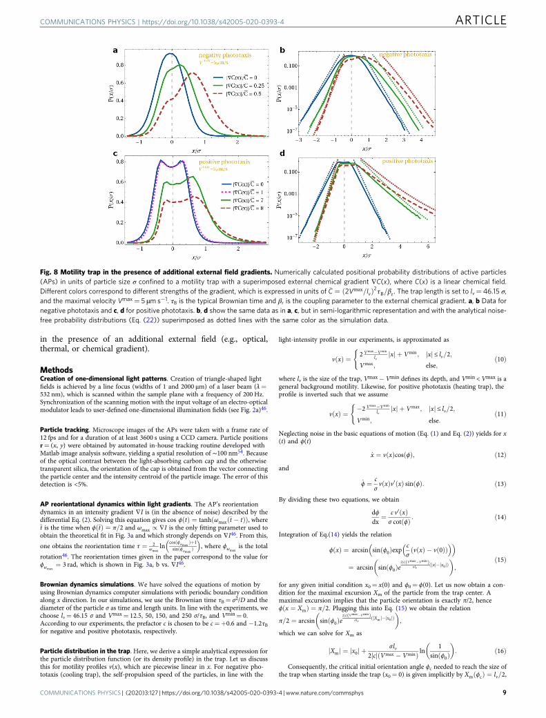
Fig. 8 Motility trap in the presence of additional external field gradients. Numerically calculated positional probability distributions of active particles(APs) in units of particle size σ confined to a motility trap with a superimposed external chemical gradient ∇C(x), where C(x) is a linear chemical field.Different colors correspond to different strengths of the gradient, which is expressed in units of �C ¼ 2Vmax=lvð Þ2τB=βr. The trap length is set to lv= 46.15 σ,and the maximal velocity Vmax= 5 µm s−1. τB is the typical Brownian time and βr is the coupling parameter to the external chemical gradient. a, b Data fornegative phototaxis and c, d for positive phototaxis. b, d show the same data as in a, c, but in semi-logarithmic representation and with the analytical noise-free probability distributions (Eq. (22)) superimposed as dotted lines with the same color as the simulation data.





which yields

ϕc ¼ ϕ0 Xm ¼ lv=2ð Þ ¼ arcsinðe� cj jΔv=σÞ: ð17ÞNow to obtain the particle distribution P(x) in the trap, we make two

assumptions. First, we assume that the particle orientation is almost homogeneouslydistributed when the particle is in the trap center. This first assumption isreasonable since there is no torque when x0= 0 and noise leads to a furthersmearing of orientations. Moreover, this assumption is found in our simulations to alarge extent. Second, we assume that the main weight in the particle distribution P(x) is given by the particle trajectory when it is stationary in x, that is, when it isturning at x= Xm. In particular, this is a good approximation for the wings of theparticle distribution, which are dominated by the turning events. Consequently, weset PðxÞ � ~PðXmÞ, where ~PðXmÞ is the distribution of the maximal excursions. Thehomogeneous distribution of initial angles then simply transforms into ~P Xmð Þ via

~P Xmð Þ ¼ 1π

dϕ0dXm

�� ¼ 2 cj j Vmax � Vminð Þ

σπlv

exp �2 cj j Vmax�Vminð Þσlv

Xmj j� �

ffiffiffiffiffiffiffiffiffiffiffiffiffiffiffiffiffiffiffiffiffiffiffiffiffiffiffiffiffiffiffiffiffiffiffiffiffiffiffiffiffiffiffiffiffiffiffiffiffiffiffiffiffiffiffiffiffiffiffi1� exp �4 cj j Vmax�Vminð Þ

σlvXmj j

� �r ; ð18Þ

which directly yields Eq. (3).These trapping mechanisms can be used as a sensor of an external field.

Specifically, in case of chemotactic rotational motion in the vicinity of the chemicalfield C(x), the rotational Langevin Eq. (2) goes to

_ϕ tð Þ ¼ cσv xð Þv0 xð Þ sin ϕþ ffiffiffiffiffiffiffiffi

2Dr

pξϕ tð Þ � βrC

0 xð Þsin ϕ; ð19Þwhere β(r) denotes the rotational chemotactic coupling coefficient. Therefore, incase of vanishing noise, the relation between ϕ(t) and x(t) is obtained as

sin ϕ xð Þð Þ ¼ sinðϕ0Þexp 2cΔvσlv

xj j � x0j jð Þ � βrC xð Þv xð Þ

þ βrC x0ð Þv x0ð Þ � βr

Z x

x0

dx0Cðx0Þv2ðx0Þ v

0ðx0Þ!;

ð20Þ

which yields Eq. (15) when βr= 0. That is to say, by knowing C(x) and solving theintegral on r.h.s., one can find the probability distribution P(x) in the presence ofchemotaxis. For instance, in case of a linear chemical field C(x)= hx+ h0, Eq. (20)goes to

sin ϕ xð Þð Þ ¼ sinðϕ0Þvð0ÞvðxÞ� h βr

v0 ðxÞexp

�cσ

v xð Þ � v 0ð Þð Þ�βrhxv xð Þ �

h βrv0ðxÞ

vð0ÞvðxÞ � 1

� ;

ð21Þwith x0= 0. Following the same assumptions and similar calculations giving rise tothe derivation of Eq. (3) from Eq. (15), Eq. (21) yields the noise-free probabilitydistribution in the vicinity of the linear chemical field

P xð Þ ’π�1 dB x;hð Þ

dx

�� ffiffiffiffiffiffiffiffiffiffiffiffiffiffiffiffiffiffiffiffiffiffiffiffi1� B2 x; hð Þp ; ð22Þ

with B(x, h) given by Eq. (9). This probability distribution is biased due to thepresence of the external chemical gradient. It can be used for indirectmeasurements of coupling coefficients of APs to external gradients (or gradientsproduced by other APs50–53). This can be done by measuring the AP distributionin a motility trap in the presence of an additional external chemical gradient (oranalogously a thermal or intensity gradient). When matching the flanks of thepredicted distribution (Eq. (22)), which depend uniquely on βr (Fig. 8) to themeasured ones, this allows to determine βr. In Fig. 8, we show the AP distributionfor different reduced chemical gradients ∇Cj j=�C, where �C ¼ 2Vmax=lvð Þ2τB=βr.

Data availabilityThe data that support the findings of this study are available from the correspondingauthor upon reasonable request.

Code availabilityThe code that supports the findings of this study are available from the correspondingauthor upon request.

Received: 9 March 2020; Accepted: 18 June 2020;

References1. Anderson, M. H., Ensher, J. R., Matthews, M. R., Wieman, C. E. & Cornell, E. A.

Observation of Bose–Einstein condensation in a dilute atomic vapor. Science 269,198–201 (1995).

2. Davis, K. B., Mewes, M.-O., Joffe, M. A., Andrews, M. R. & Ketterle, W.Evaporative cooling of sodium atoms. Phys. Rev. Lett. 75, 2909 (1995).

3. Davis, K. B. et al. Bose–Einstein condensation in a gas of sodium atoms. Phys.Rev. Lett. 75, 3969–3973 (1995).

4. Cirac, J. I. & Zoller, P. Quantum computations with cold trapped ions. Phys.Rev. Lett. 74, 4091–4094 (1995).

5. Blatt, R. & Wineland, D. Entangled states of trapped atomic ions. Nature 453,1008–1015 (2008).

6. Ashkin, A. & Dziedzic, J. M. Optical trapping and manipulation of viruses andbacteria. Science 235, 1517–1520 (1987).

7. Grier, D. G. A revolution in optical manipulation. Nature 424, 810–816(2003).

8. Wang, M. D., Yin, H., Landick, R., Gelles, J. & Block, S. M. Stretching DNAwith optical tweezers. Biophys. J. 72, 1335–1346 (1997).

9. Bechinger, C. et al. Active particles in complex and crowded environments.Rev. Mod. Phys. 88, 045006 (2016).

10. Marchetti, M. C. et al. Hydrodynamics of soft active matter. Rev. Mod. Phys.85, 1143–1189 (2013).

11. Zöttl, A. & Stark, H. Emergent behavior in active colloids. J. Phys. Condens.Matter 28, 253001 (2016).

12. Ebbens, S. J. Active colloids: progress and challenges towards realisingautonomous applications. Curr. Opin. Colloid Interface Sci. 21, 14–23(2016).

13. Ginot, F., Theurkauff, I., Detcheverry, F., Ybert, C. & Cottin-Bizonne, C.Aggregation–fragmentation and individual dynamics of active clusters. Nat.Commun. 9, 696 (2018).

14. Paxton, W. F. et al. Catalytic nanomotors: autonomous movement of stripednanorods. J. Am. Chem. Soc. 126, 13424–13431 (2004).

15. Jiang, H.-R., Yoshinaga, N. & Sano, M. Active motion of a Janus particle byself-thermophoresis in a defocused laser beam. Phys. Rev. Lett. 105, 268302(2010).

16. Elgeti, J., Winkler, R. G. & Gompper, G. Physics of microswimmers–singleparticle motion and collective behavior: a review. Rep. Prog. Phys. 78, 056601(2015).

17. Lozano, C. & Bechinger, C. Diffusing wave paradox of phototactic particles intraveling light pulses. Nat. Commun. 10, 2495 (2019).

18. Palacci, J. et al. Artificial rheotaxis. Sci. Adv. 1, e1400214 (2015).19. Lavergne, F. A., Wendehenne, H., Bäuerle, T. & Bechinger, C. Group

formation and cohesion of active particles with visual perception-dependentmotility. Science 364, 70–74 (2019).

20. Bäuerle, T., Fischer, A., Speck, T. & Bechinger, C. Self-organization of activeparticles by quorum sensing rules. Nat. Commun. 9, 3232 (2018).

21. Ma, X., Hahn, K. & Sanchez, S. Catalytic mesoporous Janus nanomotors foractive cargo delivery. J. Am. Chem. Soc. 137, 4976–4979 (2015).

22. Demirörs, A. F., Akan, M. T., Poloni, E. & Studart, A. R. Active cargotransport with Janus colloidal shuttles using electric and magnetic fields. SoftMatter 14, 4741–4749 (2018).

23. Mano, T., Delfau, J.-B., Iwasawa, J. & Sano, M. Optimal run-and-tumble-basedtransportation of a Janus particle with active steering. Proc. Natl Acad. Sci.USA 114, E2580–E2589 (2017).

24. Kumar, N., Gupta, R. K., Soni, H., Ramaswamy, S. & Sood, A. K. Trapping andsorting active particles: motility-induced condensation and smectic defects.Phys. Rev. E 99, 032605 (2019).

25. Guidobaldi, A. et al. Geometrical guidance and trapping transition of humansperm cells. Phys. Rev. E 89, 032720 (2014).

26. Restrepo-Pérez, L., Soler, L., Martínez-Cisneros, C. S., Sánchez, S. & Schmidt, O. G.Trapping self-propelled micromotors with microfabricated chevron and heart-shaped chips. Lab Chip 14, 1515–1518 (2014).

27. Thalhammer, G. et al. Combined acoustic and optical trapping. Biomed. Opt.Express 2, 2859 (2011).

28. Dauchot, O. & Démery, V. Dynamics of a self-propelled particle in aharmonic trap. Phys. Rev. Lett. 122, 068002 (2019).

29. Simmchen, J. et al. Topographical pathways guide chemical microswimmers.Nat. Commun. 7, 10598 (2016).

30. Volpe, G., Buttinoni, I., Vogt, D., Kümmerer, H.-J. & Bechinger, C.Microswimmers in patterned environments. Soft Matter 7, 8810 (2011).

31. Kaiser, A., Wensink, H. H. & Löwen, H. How to capture active particles. Phys.Rev. Lett. 108, 268307 (2012).

32. Jones, P., Marago, O. & Volpe, G. Optical Tweezers: Principles andApplications (Cambridge Univ. Press, Cambridge, 2015) .

33. Liu, J. & Li, Z. Controlled mechanical motions of microparticles in opticaltweezers. Micromachines 9, 232 (2018).

34. Zong, Y. et al. An optically driven bistable Janus rotor with patterned metalcoatings. ACS Nano 9, 10844–10851 (2015).

35. Nedev, S. et al. An optically controlled microscale elevator using plasmonicJanus particles. ACS Photonics 2, 491–496 (2015).

36. Liu, J., Guo, H.-L. & Li, Z.-Y. Self-propelled round-trip motion of Janusparticles in static line optical tweezers. Nanoscale 8, 19894–19900 (2016).




37. Moyses, H., Palacci, J., Sacanna, S. & Grier, D. G. Trochoidal trajectories ofself-propelled Janus particles in a diverging laser beam. Soft Matter 12,6357–6364 (2016).

38. Mousavi, S. M. et al. Clustering of Janus particles in an optical potential drivenby hydrodynamic fluxes. Soft Matter 15, 5748–5759 (2019).

39. Bregulla, A. P., Yang, H. & Cichos, F. Stochastic localization ofmicroswimmers by photon nudging. ACS Nano 8, 6542–6550 (2014).

40. Takatori, S. C., De Dier, R., Vermant, J. & Brady, J. F. Acoustic trapping ofactive matter. Nat. Commun. 7, 10694 (2016).

41. Soto, R. & Golestanian, R. Run-and-tumble dynamics in a crowdedenvironment: persistent exclusion process for swimmers. Phys. Rev. E 89,012706 (2014).

42. Howse, J. R. et al. Self-motile colloidal particles: from directed propulsion torandom walk. Phys. Rev. Lett. 99, 048102 (2007).

43. Gomez-Solano, J. R. et al. Tuning the motility and directionality of self-propelled colloids. Sci. Rep. 7, 14891 (2017).

44. Buttinoni, I., Volpe, G., Kümmel, F., Volpe, G. & Bechinger, C. ActiveBrownian motion tunable by light. J. Phys. Condens. Matter 24, 284129 (2012).

45. Samin, S. & van Roij, R. Self-propulsion mechanism of active Janus particles innear-critical binary mixtures. Phys. Rev. Lett. 115, 188305 (2015).

46. Lozano, C., Ten Hagen, B., Löwen, H. & Bechinger, C. Phototaxis of syntheticmicroswimmers in optical landscapes. Nat. Commun. 7, 12828 (2016).

47. Anderson, J. Colloid transport by interfacial forces. Annu. Rev. Fluid Mech. 21,61–99 (1989).

48. Phillips, W. D. Laser cooling and trapping of neutral atoms. Rev. Mod. Phys.40, https://doi.org/10.21236/ada253730 (1992).

49. Cates, M. E. & Tailleur, J. Motility-induced phase separation. Annu. Rev.Condens. Matter Phys. 6, 219–244 (2015).

50. Liebchen, B. & Löwen, H. Synthetic chemotaxis and collective behavior inactive matter. Acc. Chem. Res. 51, 2982–2990 (2018).

51. Saha, S., Golestanian, R. & Ramaswamy, S. Clusters, asters, and collectiveoscillations in chemotactic colloids. Phys. Rev. E 89, 062316 (2014).

52. Liebchen, B., Marenduzzo, D., Pagonabarraga, I. & Cates, M. E. Clustering andpattern formation in chemorepulsive active colloids. Phys. Rev. Lett. 115,258301 (2015).

53. Pohl, O. & Stark, H. Dynamic clustering and chemotactic collapse of self-phoretic active particles. Phys. Rev. Lett. 112, 238303 (2014).

54. Lozano, C., Gomez-Solano, J. R. & Bechinger, C. Run-and-tumble-like motionof active colloids in viscoelastic media. N. J. Phys. 20, 015008 (2018).

AcknowledgementsC.B. acknowledges financial support by the ERC Advanced Grant ASCIR (Grant No.693683). C.B and H.L. acknowledge support from the German Research Foundation(DFG) through the priority program SPP 1726.

Author contributionsC.L., C.B., and H.L. have planned the project. S.J./B.L. and C.L. have performed thetheoretical and experimental research, respectively. All authors have discussed andinterpreted the results and have written and edited the manuscript.

Competing interestsThe authors declare no competing interests.

Additional informationCorrespondence and requests for materials should be addressed to C.B.

Reprints and permission information is available at http://www.nature.com/reprints

Publisher’s note Springer Nature remains neutral with regard to jurisdictional claims inpublished maps and institutional affiliations.

Open Access This article is licensed under a Creative CommonsAttribution 4.0 International License, which permits use, sharing,

adaptation, distribution and reproduction in any medium or format, as long as you giveappropriate credit to the original author(s) and the source, provide a link to the CreativeCommons license, and indicate if changes were made. The images or other third partymaterial in this article are included in the article’s Creative Commons license, unlessindicated otherwise in a credit line to the material. If material is not included in thearticle’s Creative Commons license and your intended use is not permitted by statutoryregulation or exceeds the permitted use, you will need to obtain permission directly fromthe copyright holder. To view a copy of this license, visit http://creativecommons.org/licenses/by/4.0/.

© The Author(s) 2020



https://doi.org/10.21236/ada253730

http://www.nature.com/reprints

http://creativecommons.org/licenses/by/4.0/

http://creativecommons.org/licenses/by/4.0/



Documents

Realization of a motility-trap for active particles