Embed Size (px)
Citation preview
Realisation of a Digitally Scanned Laser Light
Sheet Fluorescence Microscope (DSLM)
with determination of System Resolution
Author James Anthony Seyforth
Supervisor Dr Simon Ameer-Beg
7CCP4000 Project in Physics
SUBMITTED TO THE DEPARTMENT OF PHYSICS IN PARTIAL FULFILLMENT OF THE
REQUIREMENTS FOR THE DEGREE OF
INTEGRATED MASTER OF SCIENCE
AT
KING'S COLLEGE LONDON
Date of submission: April 21, 2016

Abstract
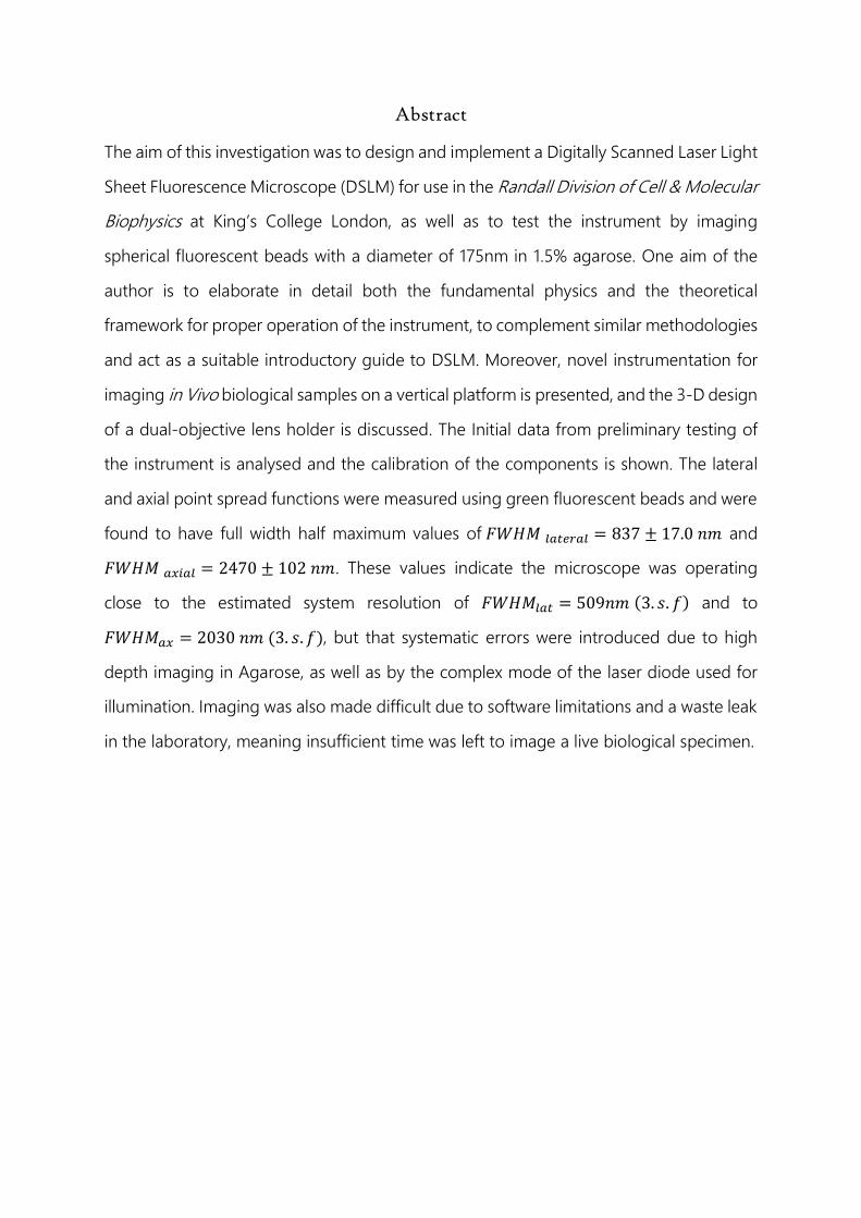
The aim of this investigation was to design and implement a Digitally Scanned Laser Light
Sheet Fluorescence Microscope (DSLM) for use in the Randall Division of Cell & Molecular
Biophysics at King’s College London, as well as to test the instrument by imaging
spherical fluorescent beads with a diameter of 175nm in 1.5% agarose. One aim of the
author is to elaborate in detail both the fundamental physics and the theoretical
framework for proper operation of the instrument, to complement similar methodologies
and act as a suitable introductory guide to DSLM. Moreover, novel instrumentation for
imaging in Vivo biological samples on a vertical platform is presented, and the 3-D design
of a dual-objective lens holder is discussed. The Initial data from preliminary testing of
the instrument is analysed and the calibration of the components is shown. The lateral
and axial point spread functions were measured using green fluorescent beads and were
found to have full width half maximum values of 𝐹𝑊𝐻𝑀 𝑙𝑎𝑡𝑒𝑟𝑎𝑙 = 837 ± 17.0 𝑛𝑚 and
𝐹𝑊𝐻𝑀 𝑎𝑥𝑖𝑎𝑙 = 2470 ± 102 𝑛𝑚. These values indicate the microscope was operating
close to the estimated system resolution of 𝐹𝑊𝐻𝑀𝑙𝑎𝑡 = 509𝑛𝑚 (3. 𝑠. 𝑓) and to
𝐹𝑊𝐻𝑀𝑎𝑥 = 2030 𝑛𝑚 (3. 𝑠. 𝑓), but that systematic errors were introduced due to high
depth imaging in Agarose, as well as by the complex mode of the laser diode used for
illumination. Imaging was also made difficult due to software limitations and a waste leak
in the laboratory, meaning insufficient time was left to image a live biological specimen.

Contents 1 Introduction ........................................................................................................................................ - 1 -
1.1 Selective Plane Illumination Microscopy ............................................................................ - 2 -
1.2 The Fundamental Physics of DSLM .................................................................................... - 4 -
1.2 The Physical Characteristics of Gaussian Beams ................................................................ - 6 -
1.4 The Paraxial Approximation and Geometric Optics........................................................... - 9 -
1.5 Infinity Corrected Microscopic Objectives ........................................................................ - 10 -
1.6 Resolution and the Point Spread Function (PSF) .............................................................. - 13 -
2 Method ............................................................................................................................................... - 17 -
2.1 Optical set-up for DSLM .................................................................................................... - 18 -
2.2 LASER Illumination ........................................................................................................... - 20 -
2.3 Characterising the Laser Light Sheet.................................................................................. - 23 -
2.4 Beam Magnification ............................................................................................................ - 24 -
2.5 The System Point Spread Function .................................................................................... - 25 -
2.6 Digitally Scanned Galvanometers and the Scanning Angle ............................................. - 26 -
2.7 Piezoelectric Flexure Objective Scanner ............................................................................ - 27 -
2.8 3D Printed Dual-Objective Lens-Holder ........................................................................... - 27 -
2.8 Fluorescence Detection and Digital Image Acquisition .................................................... - 30 -
2.9 Synchronising the Z-Galvo and the Objective Piezo ........................................................ - 32 -
2.10 Signal Generation and LabVIEW Control Software ...................................................... - 36 -
2.11 Sample Preparation ........................................................................................................... - 38 -
3 Results & Analysis ........................................................................................................................ - 40 -
3.1 Initial Gaussian Light Sheet Characterisation ................................................................... - 40 -
3.2 Optimization of the System Resolution ............................................................................. - 41 -
3.3 Discussion of Results .......................................................................................................... - 47 -
3.4 Conclusions ......................................................................................................................... - 51 -
Acknowledgments ..............................................................................................................................- 52 -
References .............................................................................................................................................- 53 -
APPENDIX A ....................................................................................................................................- 56 -
APPENDIX B .....................................................................................................................................- 58 -
APPENDIX C ....................................................................................................................................- 59 -
APPENDIX D ....................................................................................................................................- 60 -

D i g i t a l l y S c a n n e d L a s e r L i g h t S h e e t F l u o r e s c e n c e M i c r o s c o p y | - 1 -|
J a m e s A n t h o n y S e y f o r t h K i n g ’ s C o l l e g e L o n d o n , A p r i l 2 0 1 6
1 Introduction
The Biological sciences are increasingly reliant upon biophysical and quantitative analysis,
and the methods to do such analyses have exploded with the advent of the computing
age [1]. Over the last thirty years, one such method that has steadily improved is Confocal
Fluorescence Microscopy (CFM), which has given biologists the ability to optically section
biological specimens and create 3D “virtual” representations of biological systems.
However, although CFM has been successful, it delivers a high light dose to the sample,
causing high photo-toxicity and damage to cells. Moreover, because biological
specimens are extremely sensitive to their environment, CFM struggles to deliver high
resolution beyond ~30 µm depth into a sample for in vivo biological specimens. But CFM
has been of paramount importance for investigating hypothesised mechanisms and
pathways such as morphogens and gene expression. However, a new technique called
Selective Plane Illumination Microscopy (SPIM) may have solved some of these problems;
SPIM microscopes illuminate samples as little as possible using a laser ‘light-sheet’, whilst
detecting fluorescence as quickly as possible via wide-field photon detection. Datasets
can now be acquired at high spatial resolution over tens of hours at a time with minimal
cell damage. Using SPIM techniques, biologists are able to accurately document how
“differentiation, pattern formation and growth control…” are produced by “the form and
function of cells and tissue” [1]. Thus, had William Blake been born 200 years later,
perhaps he would have been a developmental biologist, and with the right tools, he could
have got highly illuminating answers to his questions.
Tyger Tyger, burning bright,
In the forests of the night;
What immortal hand or eye,
Could frame thy fearful symmetry?
- William Blake
D i g i t a l l y S c a n n e d L a s e r L i g h t S h e e t F l u o r e s c e n c e M i c r o s c o p y | - 2 -|
J a m e s A n t h o n y S e y f o r t h K i n g ’ s C o l l e g e L o n d o n , A p r i l 2 0 1 6
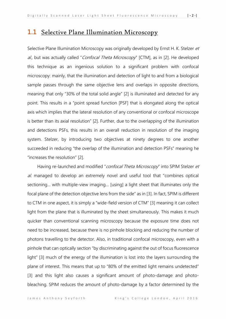
1.1 Selective Plane Illumination Microscopy
Selective Plane Illumination Microscopy was originally developed by Ernst H. K. Stelzer et
al., but was actually called “Confocal Theta Microscopy” [CTM], as in [2]. He developed
this technique as an ingenious solution to a significant problem with confocal
microscopy: mainly, that the illumination and detection of light to and from a biological
sample passes through the same objective lens and overlaps in opposite directions,
meaning that only “30% of the total solid angle” [2] is illuminated and detected for any
point. This results in a “point spread function [PSF] that is elongated along the optical
axis which implies that the lateral resolution of any conventional or confocal microscope
is better than its axial resolution” [2]. Further, due to the overlapping of the illumination
and detections PSFs, this results in an overall reduction in resolution of the imaging
system. Stelzer, by introducing two objectives at ninety degrees to one another
succeeded in reducing “the overlap of the illumination and detection PSFs” meaning he
“increases the resolution” [2].
Having re-launched and modified “confocal Theta Microscopy” into SPIM Stelzer et
al. managed to develop an extremely novel and useful tool that “combines optical
sectioning… with multiple-view imaging… [using] a light sheet that illuminates only the
focal plane of the detection objective lens from the side” as in [3]. In fact, SPIM is different
to CTM in one aspect, it is simply a “wide-field version of CTM” [3] meaning it can collect
light from the plane that is illuminated by the sheet simultaneously. This makes it much
quicker than conventional scanning microscopy because the exposure time does not
need to be increased, because there is no pinhole blocking and reducing the number of
photons travelling to the detector. Also, in traditional confocal microscopy, even with a
pinhole that can optically section “by discriminating against the out of focus fluorescence
light” [3] much of the energy of the illumination is lost into the layers surrounding the
plane of interest. This means that up to “80% of the emitted light remains undetected”
[3] and this light also causes a significant amount of photo-damage and photo-
bleaching. SPIM reduces the amount of photo-damage by a factor determined by the
D i g i t a l l y S c a n n e d L a s e r L i g h t S h e e t F l u o r e s c e n c e M i c r o s c o p y | - 3 -|
J a m e s A n t h o n y S e y f o r t h K i n g ’ s C o l l e g e L o n d o n , A p r i l 2 0 1 6
“ratio of the light sheet thickness over the specimen thickness” [3]. When acquiring a
stack, SPIM illuminates only N slices to acquire the whole dataset but confocal
microscopes must illuminate the whole volume for every plane imaged, meaning you
illuminate N2 slices for every dataset. SPIM reduces the energy load on a specimen by a
factor N, meaning SPIM has greater advantage over confocal due to the increasing factor;
this factor is proportional to the number of slices. For example, imaging an entire embryo
can decrease energy load by up to 500. For example, if the embryo is ~750 µm, and the
light sheet is ~1.5 µm thick, the number of slices N = 500 to image the specimen, which
is also the factor by which SPIM reduces the energy load [3].
The microscope constructed in this investigation is an extension of traditional SPIM,
and images a sample volume via a ‘virtual light-sheet’, which is created by vertically and
horizontally scanning a focused Gaussian beam in the plane of detection, meaning even
less light is delivered to the sample during the acquisition of the dataset. This is named
Digitally Scanned Laser Light Sheet Fluorescence Microscopy (DSLM) and as Stelzer et al.
note in Ref. [4] it has “an illumination efficiency of 95% as compared with ~ 3% in
standard light sheet microscopy”. The illumination efficiency is the ratio of the useful light
energy used for acquiring data versus the light energy not used in imaging. For example,
in traditional SPIM each sample plane is exposed to the whole light sheet during
acquisition, but in DSLM only a small segment of the plane is exposed at each moment.
At ~3%, DSLM further reduces the number of photons exposed to the sample
throughout the entire imaging process, which is useful when scanning at high speeds
because photo bleaching is reduced between frames.
D i g i t a l l y S c a n n e d L a s e r L i g h t S h e e t F l u o r e s c e n c e M i c r o s c o p y | - 4 -|
J a m e s A n t h o n y S e y f o r t h K i n g ’ s C o l l e g e L o n d o n , A p r i l 2 0 1 6
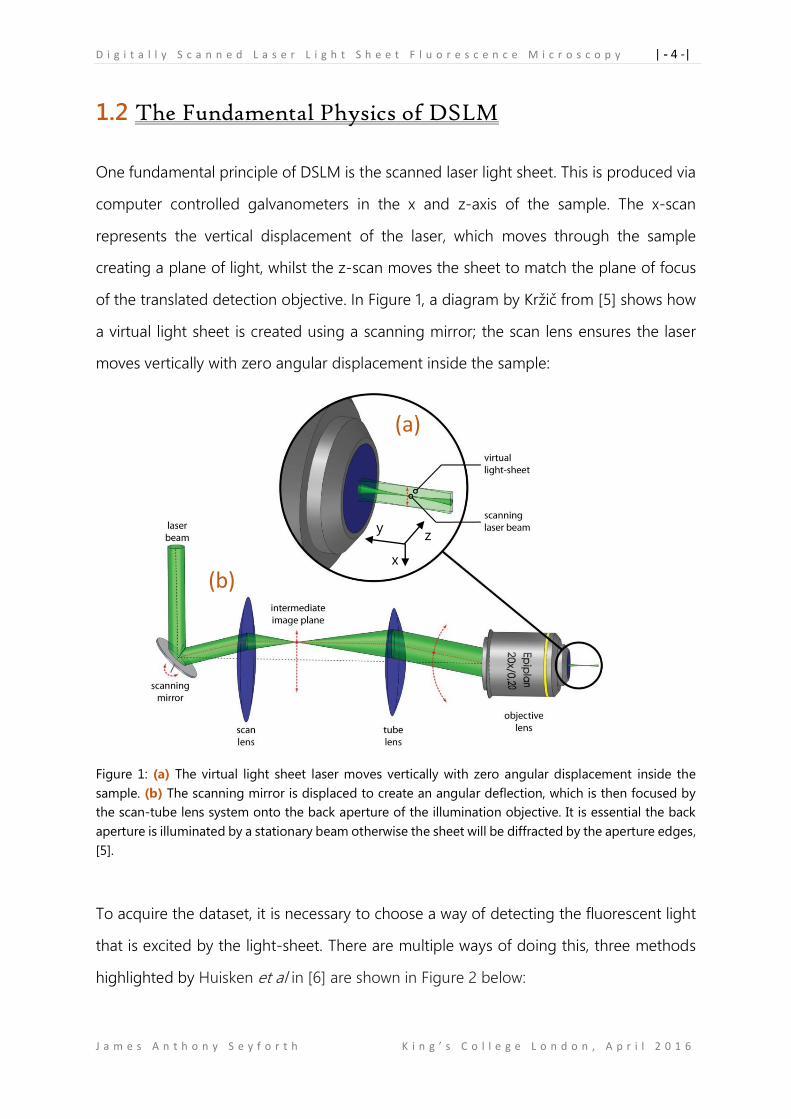
1.2 The Fundamental Physics of DSLM
One fundamental principle of DSLM is the scanned laser light sheet. This is produced via
computer controlled galvanometers in the x and z-axis of the sample. The x-scan
represents the vertical displacement of the laser, which moves through the sample
creating a plane of light, whilst the z-scan moves the sheet to match the plane of focus
of the translated detection objective. In Figure 1, a diagram by Kržič from [5] shows how
a virtual light sheet is created using a scanning mirror; the scan lens ensures the laser
moves vertically with zero angular displacement inside the sample:
Figure 1: (a) The virtual light sheet laser moves vertically with zero angular displacement inside the
sample. (b) The scanning mirror is displaced to create an angular deflection, which is then focused by
the scan-tube lens system onto the back aperture of the illumination objective. It is essential the back
aperture is illuminated by a stationary beam otherwise the sheet will be diffracted by the aperture edges,
[5].
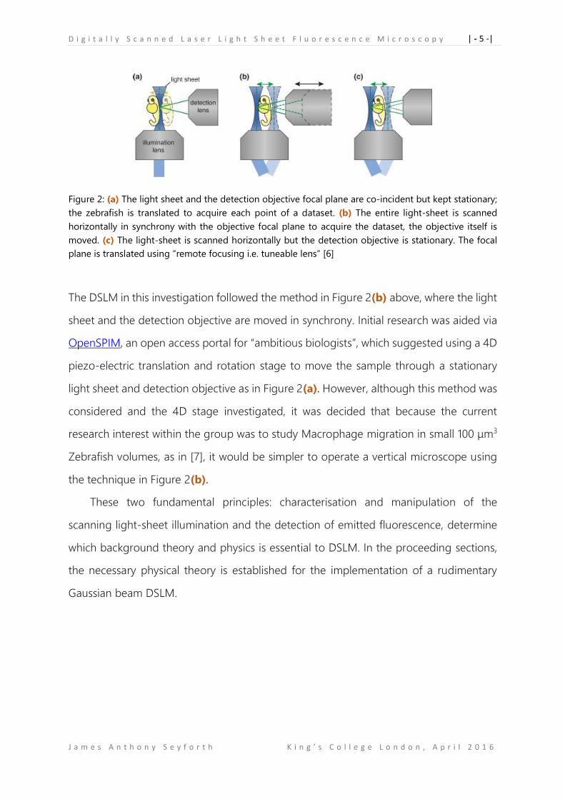
To acquire the dataset, it is necessary to choose a way of detecting the fluorescent light
that is excited by the light-sheet. There are multiple ways of doing this, three methods
highlighted by Huisken et al in [6] are shown in Figure 2 below:
(a)
(b) x
y z
D i g i t a l l y S c a n n e d L a s e r L i g h t S h e e t F l u o r e s c e n c e M i c r o s c o p y | - 5 -|
J a m e s A n t h o n y S e y f o r t h K i n g ’ s C o l l e g e L o n d o n , A p r i l 2 0 1 6
Figure 2: (a) The light sheet and the detection objective focal plane are co-incident but kept stationary;
the zebrafish is translated to acquire each point of a dataset. (b) The entire light-sheet is scanned
horizontally in synchrony with the objective focal plane to acquire the dataset, the objective itself is
moved. (c) The light-sheet is scanned horizontally but the detection objective is stationary. The focal
plane is translated using “remote focusing i.e. tuneable lens” [6]
The DSLM in this investigation followed the method in Figure 2(b) above, where the light
sheet and the detection objective are moved in synchrony. Initial research was aided via
OpenSPIM, an open access portal for “ambitious biologists”, which suggested using a 4D
piezo-electric translation and rotation stage to move the sample through a stationary
light sheet and detection objective as in Figure 2(a). However, although this method was
considered and the 4D stage investigated, it was decided that because the current
research interest within the group was to study Macrophage migration in small 100 μm3
Zebrafish volumes, as in [7], it would be simpler to operate a vertical microscope using
the technique in Figure 2(b).
These two fundamental principles: characterisation and manipulation of the
scanning light-sheet illumination and the detection of emitted fluorescence, determine
which background theory and physics is essential to DSLM. In the proceeding sections,
the necessary physical theory is established for the implementation of a rudimentary
Gaussian beam DSLM.
D i g i t a l l y S c a n n e d L a s e r L i g h t S h e e t F l u o r e s c e n c e M i c r o s c o p y | - 6 -|
J a m e s A n t h o n y S e y f o r t h K i n g ’ s C o l l e g e L o n d o n , A p r i l 2 0 1 6
1.2 The Physical Characteristics of Gaussian Beams
This DSLM utilises a Gaussian laser beam. A further reason for this is that although a
Bessel or Airy beam produce higher resolution and better optical sectioning, a Gaussian
beam is simpler to implement, and this investigation had constraints on time.
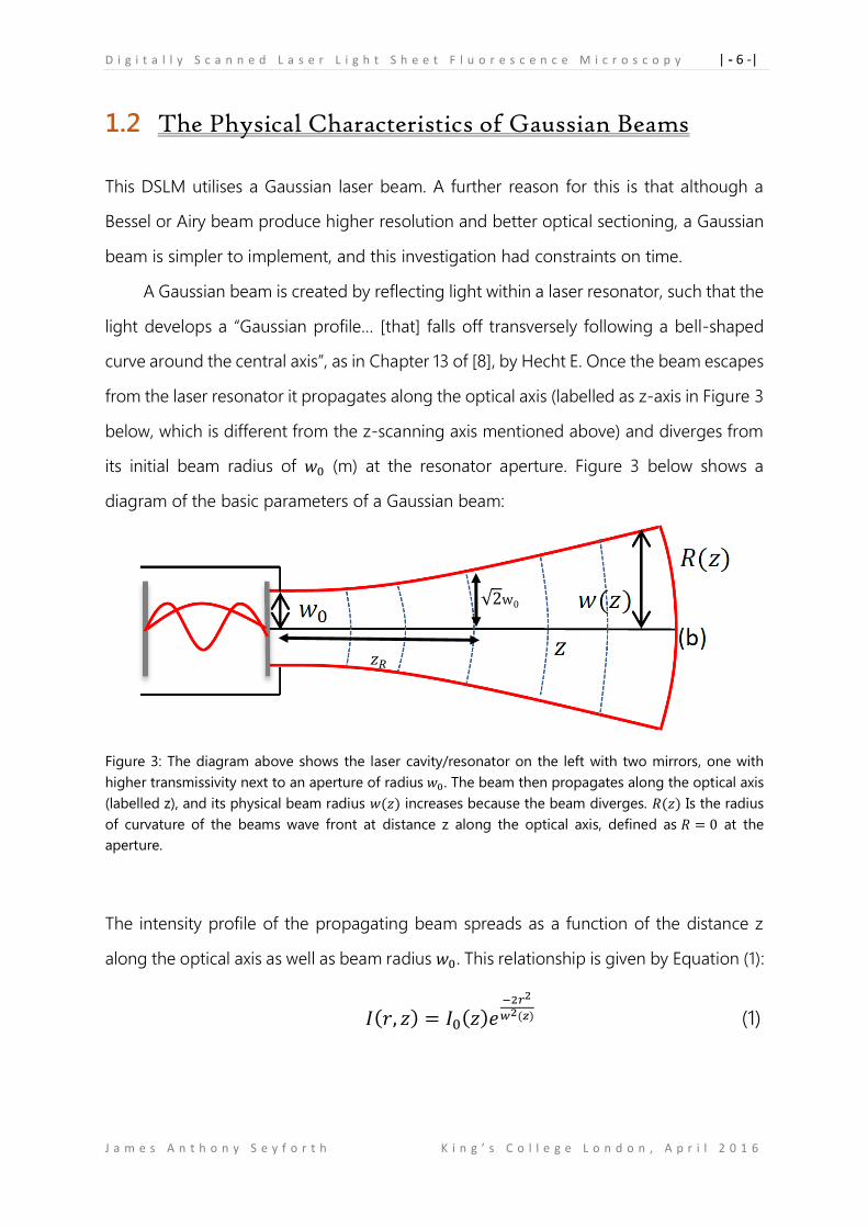
A Gaussian beam is created by reflecting light within a laser resonator, such that the
light develops a “Gaussian profile… [that] falls off transversely following a bell-shaped
curve around the central axis”, as in Chapter 13 of [8], by Hecht E. Once the beam escapes
from the laser resonator it propagates along the optical axis (labelled as z-axis in Figure 3
below, which is different from the z-scanning axis mentioned above) and diverges from
its initial beam radius of 𝑤0 (m) at the resonator aperture. Figure 3 below shows a
diagram of the basic parameters of a Gaussian beam:
Figure 3: The diagram above shows the laser cavity/resonator on the left with two mirrors, one with
higher transmissivity next to an aperture of radius 𝑤0. The beam then propagates along the optical axis
(labelled z), and its physical beam radius 𝑤(𝑧) increases because the beam diverges. 𝑅(𝑧) Is the radius
of curvature of the beams wave front at distance z along the optical axis, defined as 𝑅 = 0 at the
aperture.
The intensity profile of the propagating beam spreads as a function of the distance z
along the optical axis as well as beam radius 𝑤0. This relationship is given by Equation (1):
𝐼(𝑟, 𝑧) = 𝐼0(𝑧)𝑒−2𝑟2
𝑤2(𝑧) (1)
𝑧𝑅
√2w0
D i g i t a l l y S c a n n e d L a s e r L i g h t S h e e t F l u o r e s c e n c e M i c r o s c o p y | - 7 -|
J a m e s A n t h o n y S e y f o r t h K i n g ’ s C o l l e g e L o n d o n , A p r i l 2 0 1 6
𝐼(𝑟, 𝑧) (W/m2) is the intensity at distance 𝑧 from the resonator, and at radius 𝑟 (m) from
the central axis, 𝐼0(𝑧) is the intensity when 𝑧 = 0 and the beam radius 𝑟 = 𝑤0. 𝑤(𝑧) is
the physical beam radius and is determined by Equation (2), as defined in [8] and [9] :
𝑤(𝑧) = 𝑤0√1 + (𝜆𝑧
𝜋𝑤02)
2
= 𝑤0√1 + (𝑧
𝑧𝑅)
2
(2)
𝜆 (m) is the wavelength of the (ideal) monochromatic laser light produced in the
resonator and 𝑧𝑅 is the ‘Rayleigh Range’, defined as the distance at which the beam
radius increases by a factor of √2. I.e. 𝑧 = 𝑧𝑅 when 𝑤(𝑧) = √2𝑤0. Thus, by comparing
the two terms of the two versions of Equation (2): (𝑧2
𝑧𝑅2 =
𝜆2𝑧2
𝜋2𝑤04 ) it follows that [8]:
𝑧𝑅 =𝜋𝑤0
2
𝜆 (3)
Because the beam intensity drops off radially for whatever value of z along the
optical axis is chosen, it is necessary to determine the arbitrary beam width w(z) at value
greater than zero intensity. This is conventionally taken when 𝑟 = 𝑤(𝑧) giving a value of
𝐼 = 𝐼0/𝑒2 from Equation. (1). This arbitrary limit corresponds to a radius which contains
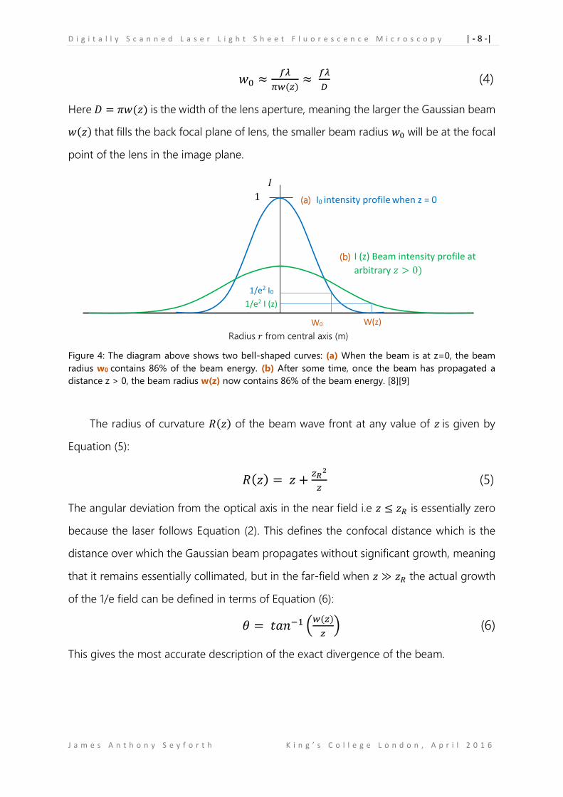
86% of the laser beam energy, as in [8]. Figure 4 shows how the bell-shaped intensity
curve widens as the beam propagates, increasing beam width.
Correct Gaussian beam focusing is essential to a properly functioning DSLM,
because if you don’t know how the lenses in any optical system interact with the beam
then you cannot accurately predict what beam radius will be produced at the focus. One
of the central theorems of Gaussian beams is that in the far-field limit when (𝑧 ≫ 𝑧𝑅), the
beam diverges linearly with increasing z, meaning its radius of curvature approximates a
spherical wave front. A fortunate consequence of this phenomenon is that for beam
focusing, one can re-apply the far-field divergence but now with the “reverse
interpretation” that the beam converges, as described in [9]. Thus the beam travels from
the lens in the far field, at beam width 𝑤(𝑓), where f stands for focal length (m), to the
beam waist 𝑤0 at 𝑓, resulting in the two equivalent approximations in Equation (4):
D i g i t a l l y S c a n n e d L a s e r L i g h t S h e e t F l u o r e s c e n c e M i c r o s c o p y | - 8 -|
J a m e s A n t h o n y S e y f o r t h K i n g ’ s C o l l e g e L o n d o n , A p r i l 2 0 1 6
𝑤0 ≈𝑓𝜆
𝜋𝑤(𝑧)≈
𝑓𝜆
𝐷 (4)
Here 𝐷 = 𝜋𝑤(𝑧) is the width of the lens aperture, meaning the larger the Gaussian beam
𝑤(𝑧) that fills the back focal plane of lens, the smaller beam radius 𝑤0 will be at the focal
point of the lens in the image plane.
Figure 4: The diagram above shows two bell-shaped curves: (a) When the beam is at z=0, the beam
radius w0 contains 86% of the beam energy. (b) After some time, once the beam has propagated a
distance z > 0, the beam radius w(z) now contains 86% of the beam energy. [8][9]
The radius of curvature 𝑅(𝑧) of the beam wave front at any value of 𝑧 is given by
Equation (5):
𝑅(𝑧) = 𝑧 +𝑧𝑅
2
𝑧 (5)
The angular deviation from the optical axis in the near field i.e 𝑧 ≤ 𝑧𝑅 is essentially zero
because the laser follows Equation (2). This defines the confocal distance which is the
distance over which the Gaussian beam propagates without significant growth, meaning
that it remains essentially collimated, but in the far-field when 𝑧 ≫ 𝑧𝑅 the actual growth
of the 1/e field can be defined in terms of Equation (6):
𝜃 = 𝑡𝑎𝑛−1 (𝑤(𝑧)
𝑧) (6)
This gives the most accurate description of the exact divergence of the beam.
1/e2 I (z)
𝐼
1 I0 intensity profile when z = 0
I (z) Beam intensity profile at
arbitrary 𝑧 > 0)
Radius 𝑟 from central axis (m)
1/e2 I0
W0 W(z)
(a)
(b)
D i g i t a l l y S c a n n e d L a s e r L i g h t S h e e t F l u o r e s c e n c e M i c r o s c o p y | - 9 -|
J a m e s A n t h o n y S e y f o r t h K i n g ’ s C o l l e g e L o n d o n , A p r i l 2 0 1 6
1.4 The Paraxial Approximation and Geometric Optics
Following the introduction to SPIM via the OpenSPIM community, it was apparent that a
full electromagnetic wave treatment or higher order optical theory would not be
necessary to align the relatively simple DSLM optical system. Under the first order or
paraxial approximation, light propagating along the optical is considered to have an
angular deviation 𝜃 small such that 𝜃 ≈ sin(𝜃) ≈ tan (𝜃). The laser beam used in this
investigation has a beam radius 𝑤0 = 350 ± 25 𝜇𝑚 and wavelength 𝜆 = 491.5 ±
0.3 𝑛𝑚 . Using Equation. (3), the Rayleigh range is found as 𝑧𝑅 = 0.78 ± 0.11 𝑚 (2.s.f),
meaning over a distance of approximately 78cm the beam is effectively collimated, as in
[10].
The paraxial approximation can be assumed because the beam will propagate
through the optical system at a distance much less than 78cm before it reaches the first
set of lenses. The beam will then be magnified to increase the beam width, which will
further decrease divergence, until finally it will be focused by the illumination objective
which will reduce the beam waist down to the 1 – 10 μm scale.
On the contrary, research into Gaussian beam optics may suggest otherwise.
For example, Sidney A. Self describes in [10] that “Because on the laboratory scale one is
often working with a lens in the near field of the incident beam, the behaviour of the
beam can be significantly different from that which would be anticipated on the basis of
geometrical optics.” However, in optical physics by Ariel Lipson et al., they describe
suggest that geometric optics does a good job “even under conditions where the
approximation is invalid!”, [11]. Perhaps it is safe to assume that the paraxial
approximation is sufficient for alignment of the beam. However, once the beam is
incident upon the tightly focusing microscopic illumination objective, a more detailed
treatment would produce a more realistic estimate of the beam propagation.
D i g i t a l l y S c a n n e d L a s e r L i g h t S h e e t F l u o r e s c e n c e M i c r o s c o p y | - 10 -|
J a m e s A n t h o n y S e y f o r t h K i n g ’ s C o l l e g e L o n d o n , A p r i l 2 0 1 6
1.5 Infinity Corrected Microscopic Objectives
Understanding how the microscopic objectives used in this investigation transform the
Gaussian beam through multiple layers of optics is essential to understanding how to
characterise a laser light sheet by illuminating the objective back aperture. Also, if the
scanning mirrors (galvanometers) are not telecentric to the back aperture of the objective
lens, the laser being scanned will be stationary, meaning it will not be parallel to the
optical axis in the sample. Thus, the beam will begin to accumulate significant angular
deflection from the optical axis and the light sheet will pivot and become non-uniform
across the field of view.
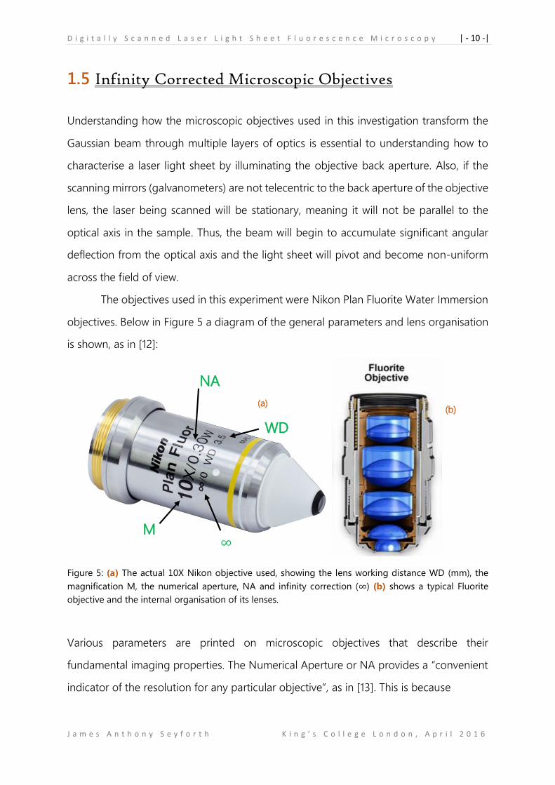
The objectives used in this experiment were Nikon Plan Fluorite Water Immersion
objectives. Below in Figure 5 a diagram of the general parameters and lens organisation
is shown, as in [12]:
Figure 5: (a) The actual 10X Nikon objective used, showing the lens working distance WD (mm), the
magnification M, the numerical aperture, NA and infinity correction (∞) (b) shows a typical Fluorite
objective and the internal organisation of its lenses.
Various parameters are printed on microscopic objectives that describe their
fundamental imaging properties. The Numerical Aperture or NA provides a “convenient
indicator of the resolution for any particular objective”, as in [13]. This is because
(b) (a)
M
NA
WD
∞
D i g i t a l l y S c a n n e d L a s e r L i g h t S h e e t F l u o r e s c e n c e M i c r o s c o p y | - 11 -|
J a m e s A n t h o n y S e y f o r t h K i n g ’ s C o l l e g e L o n d o n , A p r i l 2 0 1 6
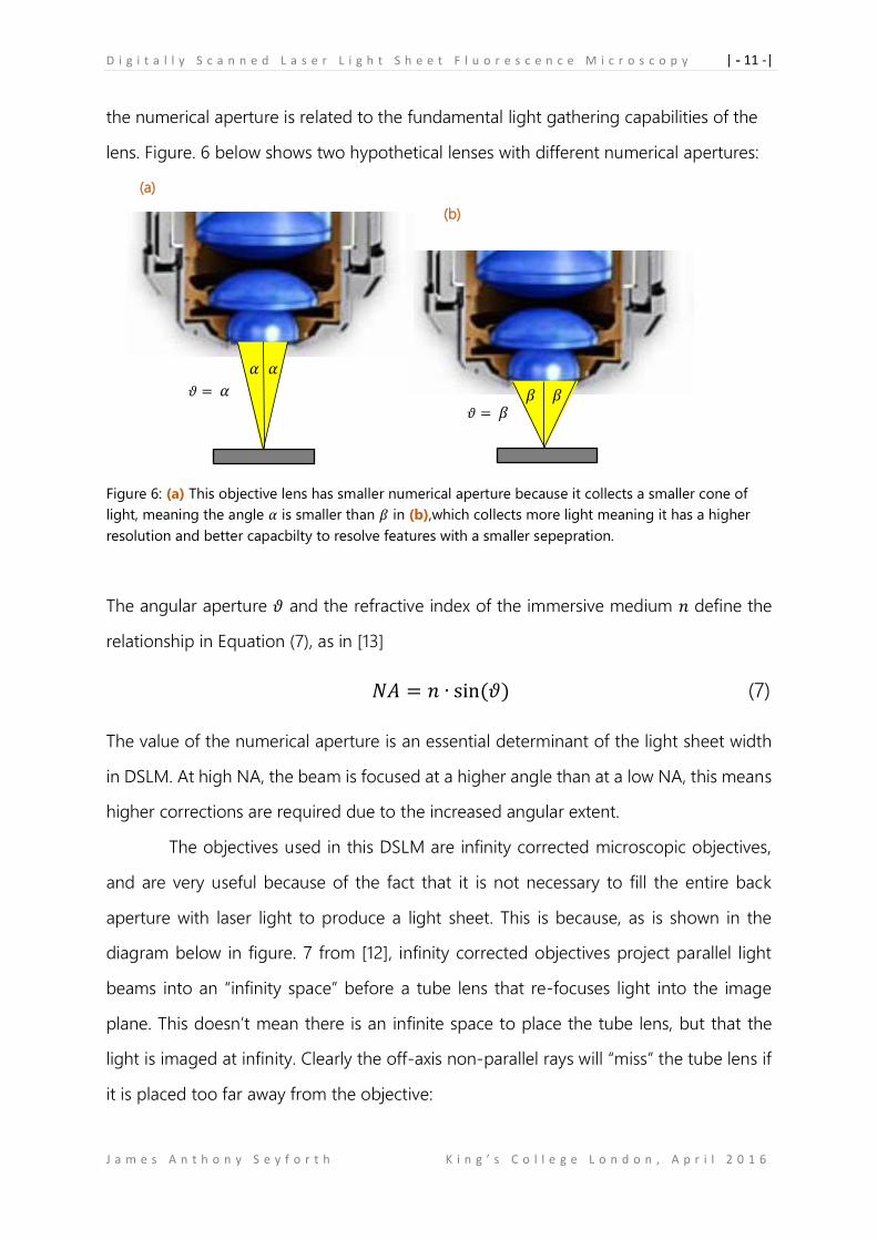
the numerical aperture is related to the fundamental light gathering capabilities of the
lens. Figure. 6 below shows two hypothetical lenses with different numerical apertures:
Figure 6: (a) This objective lens has smaller numerical aperture because it collects a smaller cone of
light, meaning the angle 𝛼 is smaller than 𝛽 in (b),which collects more light meaning it has a higher
resolution and better capacbilty to resolve features with a smaller sepepration.
The angular aperture 𝜗 and the refractive index of the immersive medium 𝑛 define the
relationship in Equation (7), as in [13]
𝑁𝐴 = 𝑛 ∙ sin (𝜗) (7)
The value of the numerical aperture is an essential determinant of the light sheet width
in DSLM. At high NA, the beam is focused at a higher angle than at a low NA, this means
higher corrections are required due to the increased angular extent.
The objectives used in this DSLM are infinity corrected microscopic objectives,
and are very useful because of the fact that it is not necessary to fill the entire back
aperture with laser light to produce a light sheet. This is because, as is shown in the
diagram below in figure. 7 from [12], infinity corrected objectives project parallel light
beams into an “infinity space” before a tube lens that re-focuses light into the image
plane. This doesn’t mean there is an infinite space to place the tube lens, but that the
light is imaged at infinity. Clearly the off-axis non-parallel rays will “miss” the tube lens if
it is placed too far away from the objective:
(a)
(b)
𝛽 𝛽
𝛼 𝛼
𝜗 = 𝛼
𝜗 = 𝛽
D i g i t a l l y S c a n n e d L a s e r L i g h t S h e e t F l u o r e s c e n c e M i c r o s c o p y | - 12 -|
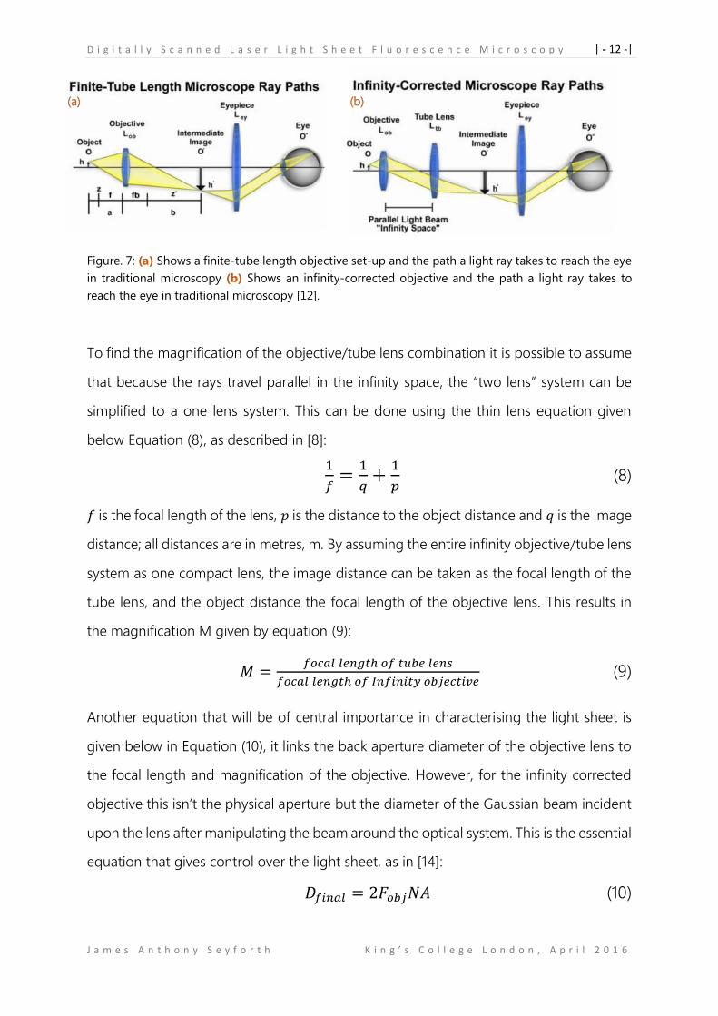
J a m e s A n t h o n y S e y f o r t h K i n g ’ s C o l l e g e L o n d o n , A p r i l 2 0 1 6
Figure. 7: (a) Shows a finite-tube length objective set-up and the path a light ray takes to reach the eye
in traditional microscopy (b) Shows an infinity-corrected objective and the path a light ray takes to
reach the eye in traditional microscopy [12].
To find the magnification of the objective/tube lens combination it is possible to assume
that because the rays travel parallel in the infinity space, the “two lens” system can be
simplified to a one lens system. This can be done using the thin lens equation given
below Equation (8), as described in [8]:
1
𝑓=
1
𝑞+
1
𝑝 (8)
𝑓 is the focal length of the lens, 𝑝 is the distance to the object distance and 𝑞 is the image
distance; all distances are in metres, m. By assuming the entire infinity objective/tube lens
system as one compact lens, the image distance can be taken as the focal length of the
tube lens, and the object distance the focal length of the objective lens. This results in
the magnification M given by equation (9):
𝑀 =𝑓𝑜𝑐𝑎𝑙 𝑙𝑒𝑛𝑔𝑡ℎ 𝑜𝑓 𝑡𝑢𝑏𝑒 𝑙𝑒𝑛𝑠
𝑓𝑜𝑐𝑎𝑙 𝑙𝑒𝑛𝑔𝑡ℎ 𝑜𝑓 𝐼𝑛𝑓𝑖𝑛𝑖𝑡𝑦 𝑜𝑏𝑗𝑒𝑐𝑡𝑖𝑣𝑒 (9)
Another equation that will be of central importance in characterising the light sheet is
given below in Equation (10), it links the back aperture diameter of the objective lens to
the focal length and magnification of the objective. However, for the infinity corrected
objective this isn’t the physical aperture but the diameter of the Gaussian beam incident
upon the lens after manipulating the beam around the optical system. This is the essential
equation that gives control over the light sheet, as in [14]:
𝐷𝑓𝑖𝑛𝑎𝑙 = 2𝐹𝑜𝑏𝑗𝑁𝐴 (10)
(a) (b)
D i g i t a l l y S c a n n e d L a s e r L i g h t S h e e t F l u o r e s c e n c e M i c r o s c o p y | - 13 -|
J a m e s A n t h o n y S e y f o r t h K i n g ’ s C o l l e g e L o n d o n , A p r i l 2 0 1 6
1.6 Resolution and the Point Spread Function (PSF)
DSLM is at the cutting edge of 3D fluorescence microscopy because it can image large
volumes with at higher speed and with greater isotropic resolution than traditional
methods such as confocal microscopy. To appreciate the manner in which DSLM achieves
this improvement, it must first be noted that “Our eyes, photographic film and electronic
image sensors only detect the intensity of the light. The image collected by the image
sensor is therefore determined by the intensity PSF”, as on page 16 in [5]. If the amplitude
PSF of the source of light is ℎ(𝑥, 𝑦, 𝑧), then the intensity PSF is given by the modulus
squared as in Equation (11) from [5]:
𝐻(𝑥, 𝑦, 𝑧) = ℎ∗(𝑥, 𝑦, 𝑧) ∙ ℎ(𝑥, 𝑦, 𝑧) = |ℎ(𝑥, 𝑦, 𝑧)|2 (11)
ℎ(𝑥, 𝑦, 𝑧) is the amplitude PSF and 𝐻(𝑥, 𝑦, 𝑧) is the intensity PSF. For both conventional
confocal microscopy and DSLM, the illumination and detection objectives both have an
associated PSF. In the case of confocal microscopy, only one objective is used and the
light travels in opposing directions, whereas for DSLM there are two objectives each with
their own PSF. This is determined according to the Stelzer-Grill-Heisenberg theory in [15],
such that the resultant intensity PSF for the DSLM optical system is Equation (12) as in
[15]:
|ℎ𝑆𝑃𝐼𝑀(𝑥, 𝑦, 𝑧)|2 = |ℎ𝑖𝑙𝑙(𝑥, 𝑦, 𝑧)|2 ∙ |ℎ𝑑𝑒𝑡(𝑥, 𝑦, 𝑧)|2 (12)
Each term is an intensity PSF which is the modulus squared of the three amplitude PSFs:
ℎ𝑆𝑃𝐼𝑀, ℎ𝑖𝑙𝑙 and ℎ𝑑𝑒𝑡 . Moreover, because the illumination and detection optical axes are at
ninety degrees to one another both PSFs overlap in a crossed pattern meaning the “PSFs
of illumination and detection optics are now elongated along two different directions,
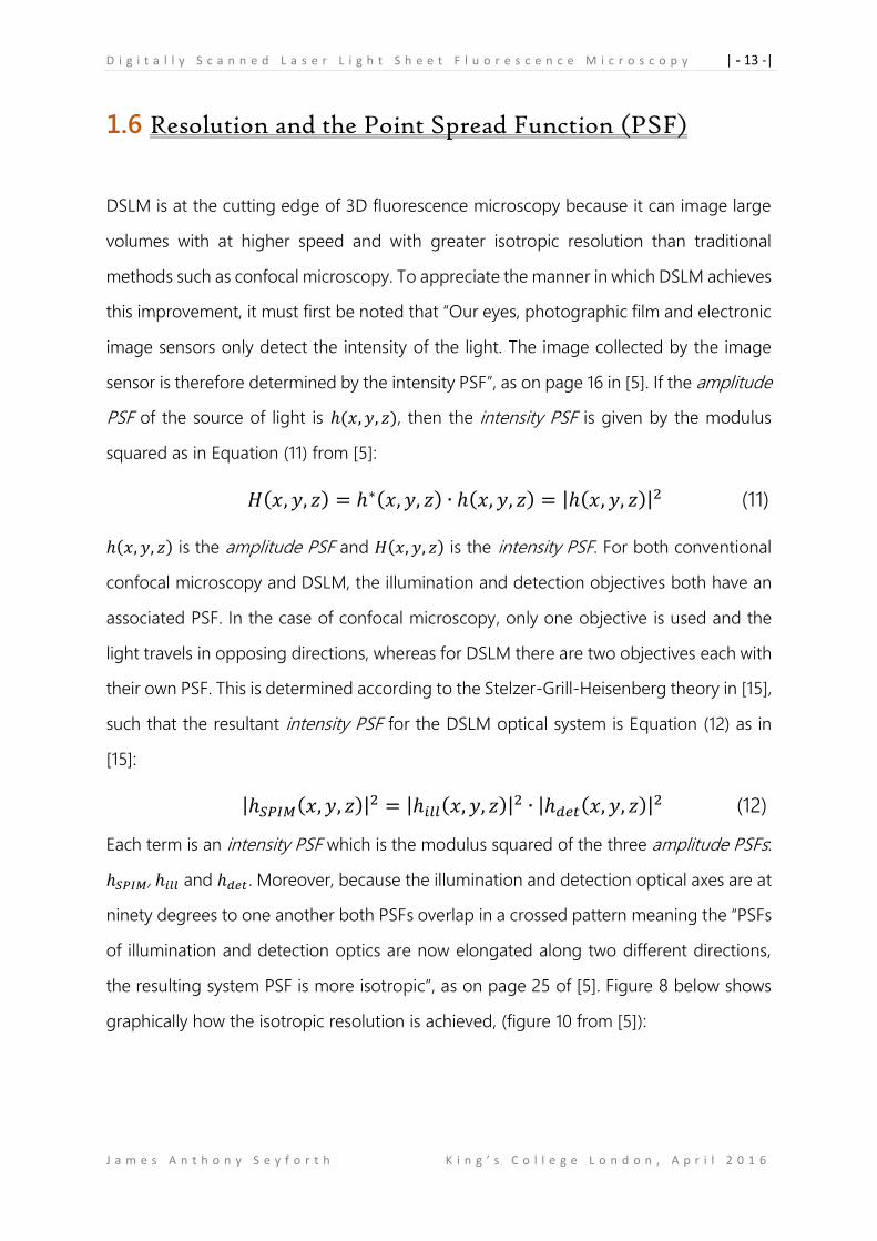
the resulting system PSF is more isotropic”, as on page 25 of [5]. Figure 8 below shows
graphically how the isotropic resolution is achieved, (figure 10 from [5]):
D i g i t a l l y S c a n n e d L a s e r L i g h t S h e e t F l u o r e s c e n c e M i c r o s c o p y | - 14 -|
J a m e s A n t h o n y S e y f o r t h K i n g ’ s C o l l e g e L o n d o n , A p r i l 2 0 1 6
Figure. 10: left The blue PSF represents illumination objective and the green PSF represnts the
detection objective as they cross inside the sample. Right multiplying both the intensity PSFs togther
gives a more isotropic PSF as shown by the two dimensonal cross for system PSF. [5]
Betzig et al. in [16] determine that for DSLM the “lateral resolution is the same as the
conventional diffraction limit of the widefield microscopy”, such that the only contributing
factor is the detection objective. To further elaborate why this is so, it is useful to recall
that the resolving power is subject to fundamental physical and not technical limits, as in
[17] and that for an image to be resolved at least half the light from the first two orders
of the Airy disk (m =±1) must reach the objective. Thus the lateral resolution is given by
the Airy disk radius 𝑟 (m) in Equation (13), from [17]:
𝑟𝑙𝑎𝑡𝑒𝑟𝑎𝑙 =1.22𝜆𝑒𝑚/𝑒𝑥𝑐
2∙𝑛∙𝑠𝑖𝑛𝜗=
0.61𝜆𝑒𝑚/𝑒𝑥𝑐
𝑁𝐴 (13)
Here 𝜆𝑒𝑚/𝑒𝑥𝑐 (m) is the wavelength of the light whether in emission or excitation and the
other parameters are as stated before. Also, the Axial Resolution is defined in Equation
(14) as in [16]
𝑟𝑎𝑥𝑖𝑎𝑙 =𝜆𝑒𝑚/𝑒𝑥𝑐
𝑛(1−cos (𝜗𝑑𝑒𝑡/𝑖𝑙𝑙) (14)
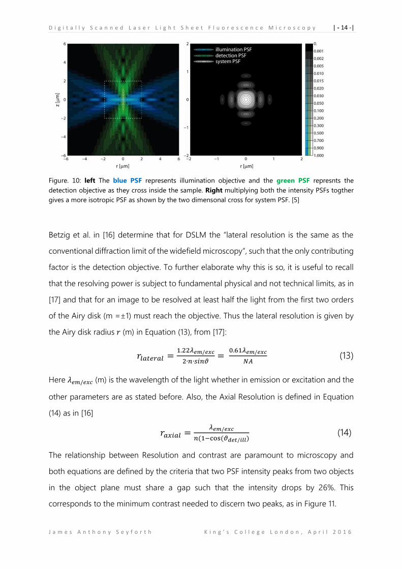
The relationship between Resolution and contrast are paramount to microscopy and
both equations are defined by the criteria that two PSF intensity peaks from two objects
in the object plane must share a gap such that the intensity drops by 26%. This
corresponds to the minimum contrast needed to discern two peaks, as in Figure 11.
D i g i t a l l y S c a n n e d L a s e r L i g h t S h e e t F l u o r e s c e n c e M i c r o s c o p y | - 15 -|
J a m e s A n t h o n y S e y f o r t h K i n g ’ s C o l l e g e L o n d o n , A p r i l 2 0 1 6
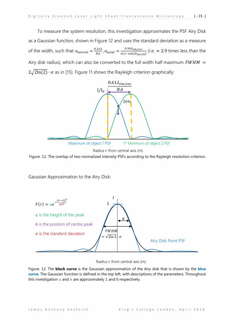
To measure the system resolution, this investigation approximates the PSF Airy Disk
as a Gaussian function, shown in Figure 12 and uses the standard deviation as a measure
of the width, such that 𝜎𝑙𝑎𝑡𝑒𝑟𝑎𝑙 =0.21𝜆
𝑁𝐴, 𝜎𝑎𝑥𝑖𝑎𝑙 =
0.34𝜆𝑒𝑚/𝑒𝑥𝑐
𝑛(1−cos (𝜗𝑑𝑒𝑡/𝑖𝑙𝑙) (i.e. ≈ 2.9 times less than the
Airy disk radius), which can also be converted to the full width half maximum 𝐹𝑊𝐻𝑀 =
2√2ln (2) ∙ 𝜎 as in [15]. Figure 11 shows the Rayleigh criterion graphically:
Figure. 11: The overlap of two normalized intensity PSFs according to the Rayleigh resolution criterion.
Gaussian Approximation to the Airy Disk:
Figure. 12: The black curve is the Gaussian approximation of the Airy disk that is shown by the blue
curve. The Gaussian function is defined in the top left, with descriptions of the parameters. Throughout
this investigation 𝑎 and 𝑏 are approximately 1 and 0 respectively.
𝐼
1 𝐹(𝑟) = 𝑎𝑒−
(𝑟−𝑏)2
2𝜎2
𝑎 is the height of the peak
𝑏 is the position of centre peak
𝜎 is the standard deviation
Airy Disk Point PSF
Radius 𝑟 from central axis (m)
𝜎
𝐹𝑊𝐻𝑀
= √2ln 2 ∙ 𝜎
Radius 𝑟 from central axis (m)
0.61𝜆𝑒𝑚/𝑒𝑥𝑐
𝑁𝐴
Maximum of object 1 PSF 1st Minimum of object 2 PSF
26%
I/I0
D i g i t a l l y S c a n n e d L a s e r L i g h t S h e e t F l u o r e s c e n c e M i c r o s c o p y | - 16 -|
J a m e s A n t h o n y S e y f o r t h K i n g ’ s C o l l e g e L o n d o n , A p r i l 2 0 1 6
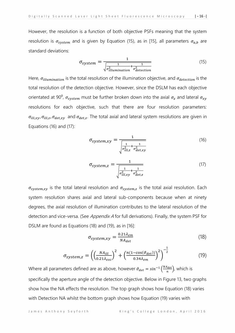
However, the resolution is a function of both objective PSFs meaning that the system
resolution is 𝜎𝑠𝑦𝑠𝑡𝑒𝑚 and is given by Equation (15), as in [15], all parameters 𝜎𝑎,𝑏 are
standard deviations:
𝜎𝑠𝑦𝑠𝑡𝑒𝑚 =1
√1
𝜎𝑖𝑙𝑙𝑢𝑚𝑖𝑛𝑎𝑡𝑖𝑜𝑛2 +
1
𝜎𝑑𝑒𝑡𝑒𝑐𝑡𝑖𝑜𝑛2
(15)
Here, 𝜎𝑖𝑙𝑙𝑢𝑚𝑖𝑛𝑎𝑡𝑖𝑜𝑛 is the total resolution of the illumination objective, and 𝜎𝑑𝑒𝑡𝑒𝑐𝑡𝑖𝑜𝑛 is the
total resolution of the detection objective. However, since the DSLM has each objective
orientated at 90⁰, 𝜎𝑠𝑦𝑠𝑡𝑒𝑚 must be further broken down into the axial 𝜎𝑧 and lateral 𝜎𝑥𝑦
resolutions for each objective, such that there are four resolution parameters:
𝜎𝑖𝑙𝑙,𝑥𝑦 , 𝜎𝑖𝑙𝑙,𝑧, 𝜎𝑑𝑒𝑡,𝑥𝑦 and 𝜎𝑑𝑒𝑡,𝑧. The total axial and lateral system resolutions are given in
Equations (16) and (17):
𝜎𝑠𝑦𝑠𝑡𝑒𝑚,𝑥𝑦 =1
√1
𝜎𝑖𝑙𝑙,𝑧2 +
1
𝜎𝑑𝑒𝑡,𝑥𝑦2
(16)
𝜎𝑠𝑦𝑠𝑡𝑒𝑚,𝑧 =1
√1
𝜎𝑖𝑙𝑙,𝑥𝑦2 +
1
𝜎𝑑𝑒𝑡,𝑧2
(17)
𝜎𝑠𝑦𝑠𝑡𝑒𝑚,𝑥𝑦 is the total lateral resolution and 𝜎𝑠𝑦𝑠𝑡𝑒𝑚,𝑧 is the total axial resolution. Each
system resolution shares axial and lateral sub-components because when at ninety
degrees, the axial resolution of illumination contributes to the lateral resolution of the
detection and vice-versa. (See Appendix A for full derivations). Finally, the system PSF for
DSLM are found as Equations (18) and (19), as in [16]:
𝜎𝑠𝑦𝑠𝑡𝑒𝑚,𝑥𝑦 =0.21𝜆𝑒𝑚
𝑁𝐴𝑑𝑒𝑡 (18)
𝜎𝑠𝑦𝑠𝑡𝑒𝑚,𝑧 = ((𝑁𝐴𝑖𝑙𝑙
0.21𝜆𝑒𝑥𝑐)
2
+ (𝑛(1−cos(𝜗𝑑𝑒𝑡))
0.34𝜆𝑒𝑚)
2)
−1
2
(19)
Where all parameters defined are as above, however 𝜗𝑑𝑒𝑡 = 𝑠𝑖𝑛−1 (𝑁𝐴𝑑𝑒𝑡
𝑛), which is
specifically the aperture angle of the detection objective. Below in Figure 13, two graphs
show how the NA effects the resolution. The top graph shows how Equation (18) varies
with Detection NA whilst the bottom graph shows how Equation (19) varies with
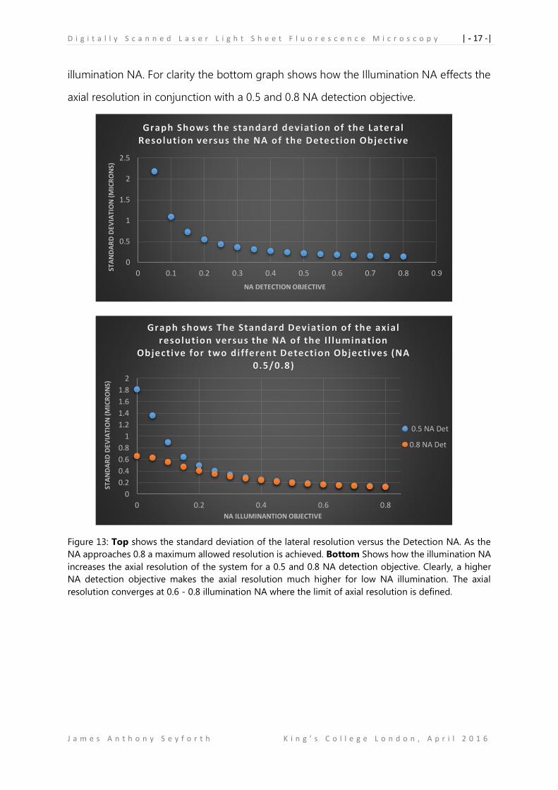
D i g i t a l l y S c a n n e d L a s e r L i g h t S h e e t F l u o r e s c e n c e M i c r o s c o p y | - 17 -|
J a m e s A n t h o n y S e y f o r t h K i n g ’ s C o l l e g e L o n d o n , A p r i l 2 0 1 6
illumination NA. For clarity the bottom graph shows how the Illumination NA effects the
axial resolution in conjunction with a 0.5 and 0.8 NA detection objective.
Figure 13: Top shows the standard deviation of the lateral resolution versus the Detection NA. As the
NA approaches 0.8 a maximum allowed resolution is achieved. Bottom Shows how the illumination NA
increases the axial resolution of the system for a 0.5 and 0.8 NA detection objective. Clearly, a higher
NA detection objective makes the axial resolution much higher for low NA illumination. The axial
resolution converges at 0.6 - 0.8 illumination NA where the limit of axial resolution is defined.
0
0.5
1
1.5
2
2.5
0 0.1 0.2 0.3 0.4 0.5 0.6 0.7 0.8 0.9
STA
ND
AR
D D
EVIA
TIO
N (M
ICR
ON
S)
NA DETECTION OBJECTIVE
Graph Shows the standard deviation of the Lateral Resolution versus the NA of the Detection Objective
0
0.2
0.4
0.6
0.8
1
1.2
1.4
1.6
1.8
2
0 0.2 0.4 0.6 0.8
STA
ND
AR
D D
EVIA
TIO
N (M
ICR
ON
S)
NA ILLUMINANTION OBJECTIVE
Graph shows The Standard Deviation of the axial resolution versus the NA of the I l lumination
Objective for two different Detection Objectives (NA 0.5/0.8)
0.5 NA Det
0.8 NA Det
D i g i t a l l y S c a n n e d L a s e r L i g h t S h e e t F l u o r e s c e n c e M i c r o s c o p y | - 18 -|
J a m e s A n t h o n y S e y f o r t h K i n g ’ s C o l l e g e L o n d o n , A p r i l 2 0 1 6
2 Method 2.1 Optical set-up for DSLM
The optical set-up for a rudimentary DSLM is remarkably simple, but serious
consideration had to be given to the method of mounting the sample. This is because
depending on the application, it may be more suitable to mount the specimen onto a
4D positioning stage and leave the objectives stationary. However, this also has
implications for the preparation of specimens which can cause various difficulties. One
such difficulty is that specimens are held vertically whilst being translated for extended
periods, which is generally an unnatural state for any sample. Also, the speed of the 4D
stage is slow, meaning acquisition time would be increased; this would limit the types of
biological phenomena that could be investigated. In addition, a custom water bath with
heating must be installed to house the objectives and the specimen as well as to allow
entrance of the 4D stage, as in OpenSPIM from [18]. Within the research group this DSLM
will be used to image how Zebrafish Macrophages respond to wounds in muscle tissue.
This means that only a volume of approximately 100 μm3 will be imaged near the surface
of the Zebrafish muscle tissue. The author concluded it was more practical for the
specimen to remain horizontally stationary, and for the optics to produce the imaging
volume. Moreover, because the specimen is now laid flat, traditional petri dishes can be
used instead of a custom made bath and the objectives can be mounted vertically as in
a traditional microscopy. The schematic for the DLSM is shown below in Figure 14.
D i g i t a l l y S c a n n e d L a s e r L i g h t S h e e t F l u o r e s c e n c e M i c r o s c o p y | - 19 -|
J a m e s A n t h o n y S e y f o r t h K i n g ’ s C o l l e g e L o n d o n , A p r i l 2 0 1 6
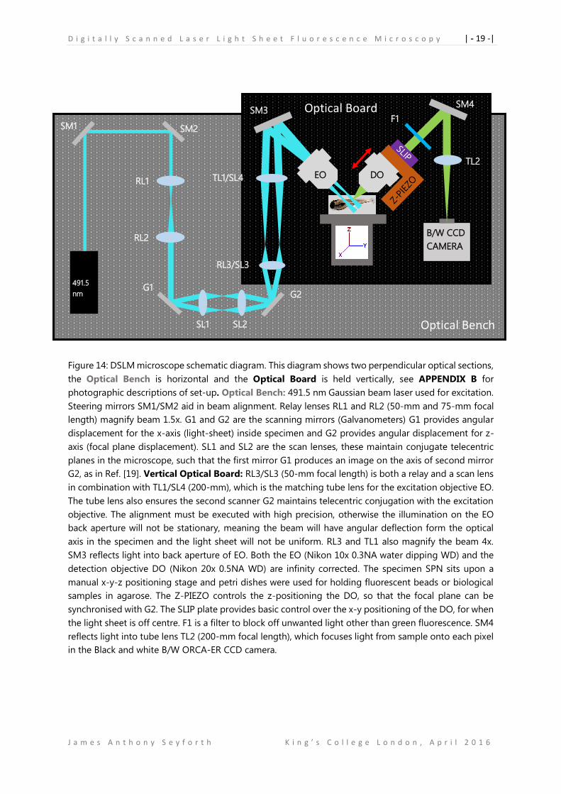
Figure 14: DSLM microscope schematic diagram. This diagram shows two perpendicular optical sections,
the Optical Bench is horizontal and the Optical Board is held vertically, see APPENDIX B for
photographic descriptions of set-up. Optical Bench: 491.5 nm Gaussian beam laser used for excitation.
Steering mirrors SM1/SM2 aid in beam alignment. Relay lenses RL1 and RL2 (50-mm and 75-mm focal
length) magnify beam 1.5x. G1 and G2 are the scanning mirrors (Galvanometers) G1 provides angular
displacement for the x-axis (light-sheet) inside specimen and G2 provides angular displacement for z-
axis (focal plane displacement). SL1 and SL2 are the scan lenses, these maintain conjugate telecentric
planes in the microscope, such that the first mirror G1 produces an image on the axis of second mirror
G2, as in Ref. [19]. Vertical Optical Board: RL3/SL3 (50-mm focal length) is both a relay and a scan lens
in combination with TL1/SL4 (200-mm), which is the matching tube lens for the excitation objective EO.
The tube lens also ensures the second scanner G2 maintains telecentric conjugation with the excitation
objective. The alignment must be executed with high precision, otherwise the illumination on the EO
back aperture will not be stationary, meaning the beam will have angular deflection form the optical
axis in the specimen and the light sheet will not be uniform. RL3 and TL1 also magnify the beam 4x.
SM3 reflects light into back aperture of EO. Both the EO (Nikon 10x 0.3NA water dipping WD) and the
detection objective DO (Nikon 20x 0.5NA WD) are infinity corrected. The specimen SPN sits upon a
manual x-y-z positioning stage and petri dishes were used for holding fluorescent beads or biological
samples in agarose. The Z-PIEZO controls the z-positioning the DO, so that the focal plane can be
synchronised with G2. The SLIP plate provides basic control over the x-y positioning of the DO, for when
the light sheet is off centre. F1 is a filter to block off unwanted light other than green fluorescence. SM4
reflects light into tube lens TL2 (200-mm focal length), which focuses light from sample onto each pixel
in the Black and white B/W ORCA-ER CCD camera.
SPN
491.5
nm
SM1 SM2
RL1
RL2
SL1 SL2
G1 G2
RL3/SL3
TL1/SL4
F1
SM4
TL2
B/W CCD
CAMERA
SM3
EO DO
Optical Bench
Optical Board
D i g i t a l l y S c a n n e d L a s e r L i g h t S h e e t F l u o r e s c e n c e M i c r o s c o p y | - 20 -|
J a m e s A n t h o n y S e y f o r t h K i n g ’ s C o l l e g e L o n d o n , A p r i l 2 0 1 6
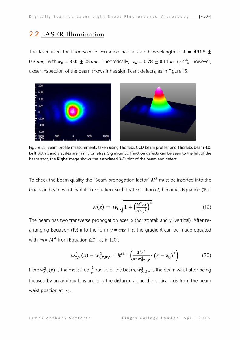
2.2 LASER Illumination
The laser used for fluorescence excitation had a stated wavelength of 𝜆 = 491.5 ±
0.3 𝑛𝑚, with 𝑤0 = 350 ± 25 𝜇𝑚. Theoretically, 𝑧𝑅 = 0.78 ± 0.11 𝑚 (2.s.f), however,
closer inspection of the beam shows it has significant defects, as in Figure 15:
Figure 15: Beam profile measurements taken using Thorlabs CCD beam profiler and Thorlabs beam 4.0.
Left Both x and y scales are in micrometres. Significant diffraction defects can be seen to the left of the
beam spot, the Right image shows the associated 3-D plot of the beam and defect.
To check the beam quality the “Beam propogation factor” 𝑀2 must be inserted into the
Guassian beam waist evolution Equation, such that Equation (2) becomes Equation (19):
𝑤(𝑧) = 𝑤0√1 + (𝑀2𝜆𝑧
𝜋𝑤02)
2
(19)
The beam has two transverse propogation axes, x (horizontal) and y (vertical). After re-
arranging Equation (19) into the form 𝑦 = 𝑚𝑥 + 𝑐, the gradient can be made equated
with 𝑚= 𝑀4 from Equation (20), as in [20]:
𝑤𝑥,𝑦2 (𝑧) − 𝑤0𝑥,0𝑦
2 = 𝑀4 ∙ (𝜆2𝑧2
𝜋2𝑤0𝑥,0𝑦4 ∙ (𝑧 − 𝑧0)2) (20)
Here 𝑤𝑥,𝑦2 (𝑧) is the measured
1
𝑒2 radius of the beam, 𝑤0𝑥,0𝑦2 is the beam waist after being
focused by an arbitray lens and 𝑧 is the distance along the optical axis from the beam
waist position at 𝑧0.
D i g i t a l l y S c a n n e d L a s e r L i g h t S h e e t F l u o r e s c e n c e M i c r o s c o p y | - 21 -|
J a m e s A n t h o n y S e y f o r t h K i n g ’ s C o l l e g e L o n d o n , A p r i l 2 0 1 6
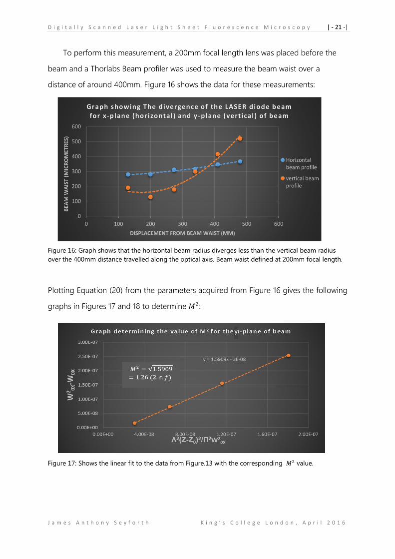
To perform this measurement, a 200mm focal length lens was placed before the
beam and a Thorlabs Beam profiler was used to measure the beam waist over a
distance of around 400mm. Figure 16 shows the data for these measurements:
Figure 16: Graph shows that the horizontal beam radius diverges less than the vertical beam radius
over the 400mm distance travelled along the optical axis. Beam waist defined at 200mm focal length.
Plotting Equation (20) from the parameters acquired from Figure 16 gives the following
graphs in Figures 17 and 18 to determine 𝑀2:
Figure 17: Shows the linear fit to the data from Figure.13 with the corresponding 𝑀2 value.
0
100
200
300
400
500
600
0 100 200 300 400 500 600
BEA
M W
AIS
T (M
ICR
OM
ETR
ES)
DISPLACEMENT FROM BEAM WAIST (MM)
Graph showing The divergence of the LASER diode beam for x-plane (horizontal) and y -plane (vertical ) of beam
Horizontalbeam profile
vertical beamprofile
y
D i g i t a l l y S c a n n e d L a s e r L i g h t S h e e t F l u o r e s c e n c e M i c r o s c o p y | - 22 -|
J a m e s A n t h o n y S e y f o r t h K i n g ’ s C o l l e g e L o n d o n , A p r i l 2 0 1 6
Figure 18: Shows the linear fit to the data from Figure.13 with the corresponding 𝑀2 value
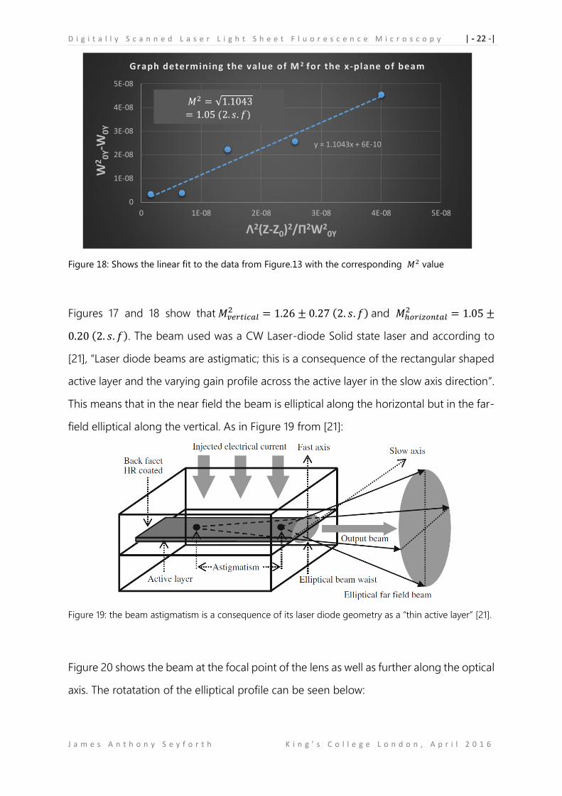
Figures 17 and 18 show that 𝑀𝑣𝑒𝑟𝑡𝑖𝑐𝑎𝑙2 = 1.26 ± 0.27 (2. 𝑠. 𝑓) and 𝑀ℎ𝑜𝑟𝑖𝑧𝑜𝑛𝑡𝑎𝑙
2 = 1.05 ±
0.20 (2. 𝑠. 𝑓). The beam used was a CW Laser-diode Solid state laser and according to
[21], “Laser diode beams are astigmatic; this is a consequence of the rectangular shaped
active layer and the varying gain profile across the active layer in the slow axis direction”.
This means that in the near field the beam is elliptical along the horizontal but in the far-
field elliptical along the vertical. As in Figure 19 from [21]:
Figure 19: the beam astigmatism is a consequence of its laser diode geometry as a “thin active layer” [21].
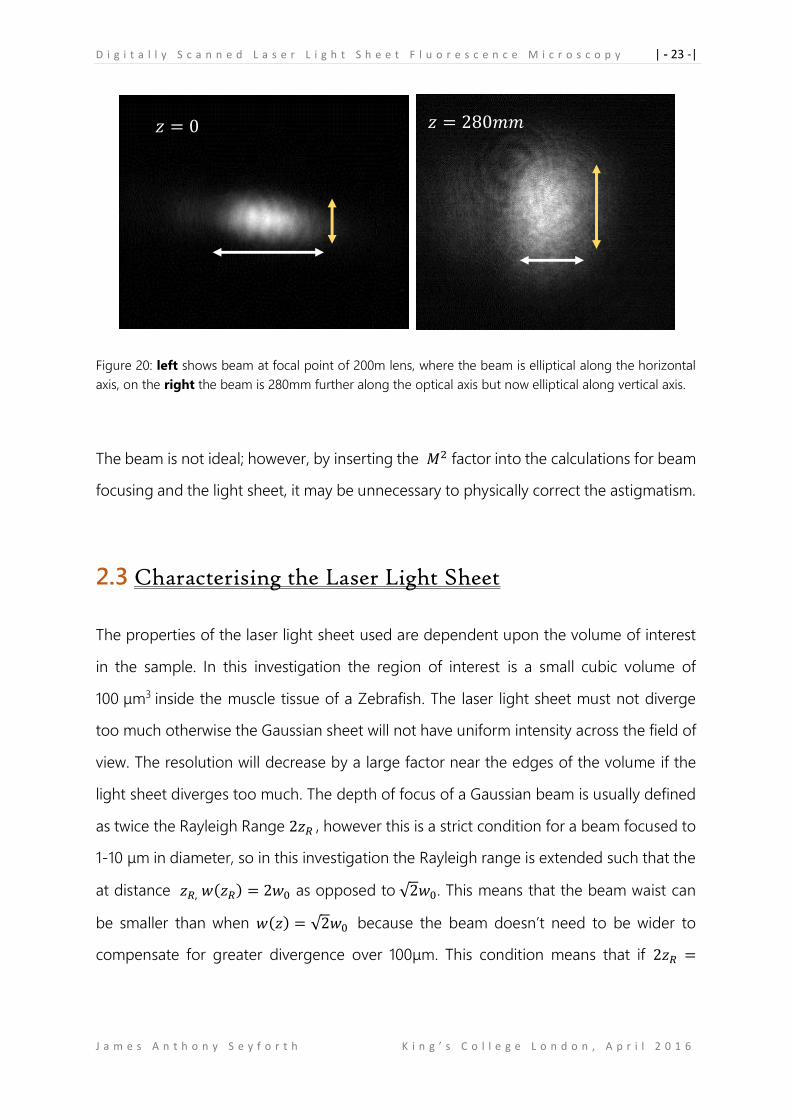
Figure 20 shows the beam at the focal point of the lens as well as further along the optical
axis. The rotatation of the elliptical profile can be seen below:
y = 1.1043x + 6E-10
0
1E-08
2E-08
3E-08
4E-08
5E-08
0 1E-08 2E-08 3E-08 4E-08 5E-08
W2
0Y-W
0Y
Λ2(Z-Z0)2/Π2W20Y
Graph determining the value of M 2 for the x-plane of beam
𝑀2 = √1.1043
= 1.05 (2. 𝑠. 𝑓)
D i g i t a l l y S c a n n e d L a s e r L i g h t S h e e t F l u o r e s c e n c e M i c r o s c o p y | - 23 -|
J a m e s A n t h o n y S e y f o r t h K i n g ’ s C o l l e g e L o n d o n , A p r i l 2 0 1 6
Figure 20: left shows beam at focal point of 200m lens, where the beam is elliptical along the horizontal
axis, on the right the beam is 280mm further along the optical axis but now elliptical along vertical axis.
The beam is not ideal; however, by inserting the 𝑀2 factor into the calculations for beam
focusing and the light sheet, it may be unnecessary to physically correct the astigmatism.
2.3 Characterising the Laser Light Sheet
The properties of the laser light sheet used are dependent upon the volume of interest
in the sample. In this investigation the region of interest is a small cubic volume of
100 μm3 inside the muscle tissue of a Zebrafish. The laser light sheet must not diverge
too much otherwise the Gaussian sheet will not have uniform intensity across the field of
view. The resolution will decrease by a large factor near the edges of the volume if the
light sheet diverges too much. The depth of focus of a Gaussian beam is usually defined
as twice the Rayleigh Range 2𝑧𝑅 , however this is a strict condition for a beam focused to
1-10 μm in diameter, so in this investigation the Rayleigh range is extended such that the
at distance 𝑧𝑅, 𝑤(𝑧𝑅) = 2𝑤0 as opposed to √2𝑤0. This means that the beam waist can
be smaller than when 𝑤(𝑧) = √2𝑤0 because the beam doesn’t need to be wider to
compensate for greater divergence over 100μm. This condition means that if 2𝑧𝑅 =
𝑧 = 0 𝑧 = 280𝑚𝑚
D i g i t a l l y S c a n n e d L a s e r L i g h t S h e e t F l u o r e s c e n c e M i c r o s c o p y | - 24 -|
J a m e s A n t h o n y S e y f o r t h K i n g ’ s C o l l e g e L o n d o n , A p r i l 2 0 1 6
100 μm then 𝑧𝑅 = 50 μm. By rearranging Equation (19) and using condition 𝑤(𝑧𝑅) =
2𝑤0, an equation linking the beam waist and Rayleigh Range is found as Equation (21):
𝑧𝑅 = ((2𝑤0)2
𝑤02 − 1)
1
2∙
𝜋𝑤02
𝜆𝑀2
𝑧𝑅 = √3 ∙𝜋𝑤0
2
𝜆𝑀2 (21)
𝑀2 is different for the vertical and horizontal axes meaning Equation (21) will also be
different for both axes. 𝑀ℎ𝑜𝑟𝑖𝑧𝑜𝑛𝑡𝑎𝑙2 = 1.05 ± 0.20 (2. 𝑠. 𝑓) and 𝑀𝑣𝑒𝑟𝑡𝑖𝑐𝑎𝑙
2 = 1.26 ±
0.27 (2. 𝑠. 𝑓). Using these values and rearranging Equation (21), the beam waists
are 𝑤0,ℎ𝑜𝑟𝑖𝑧𝑜𝑛𝑡𝑎𝑙 = 2.18 ± 0.95 𝜇𝑚 (2. 𝑠. 𝑓) and 𝑤0,𝑣𝑒𝑟𝑡𝑖𝑐𝑎𝑙 = 2.39 ± 1.06 𝜇𝑚 (2. 𝑠. 𝑓).
Here, there is uncertainty principally because of the uncertainty in 𝑀2.
The beam waists are on the micron scale and so must be focused by the 0.3 NA
Nikon illumination objective. This is done by filling the back aperture with a Gaussian
beam, of a radius that is defined by the light sheet beam waist. But since there are two
estimated waists, to approximate the filling diameter the average vertical and horizontal
beam waists were defined as 𝐷𝑖𝑙𝑙,𝑣𝑒𝑟𝑡𝑖𝑐𝑎𝑙 = 4.38 ± 1.55 𝑚𝑚 (2. 𝑠. 𝑓) and 𝐷𝑖𝑙𝑙,ℎ𝑜𝑟𝑖𝑧𝑜𝑛𝑡𝑎𝑙 =
3.82 ± 1.17 𝑚𝑚 (2. 𝑠. 𝑓). To find the filling diameter Equations (6), (7), (9) and (10) were
used to derive Equation (22). A full derivation is in APPENDIX C.:
𝐷𝑖𝑙𝑙 =2𝐹𝑜𝑏𝑗𝑛𝜆𝑀2
𝜋𝑤0
(22)
2.4 Beam Magnification
Because of the beam astigmatism, the back aperture fill diameters are 𝐷𝑖𝑙𝑙,𝑣𝑒𝑟𝑡𝑖𝑐𝑎𝑙 =
4.38 ± 1.55 𝑚𝑚 (2. 𝑠. 𝑓) and 𝐷𝑖𝑙𝑙,ℎ𝑜𝑟𝑖𝑧𝑜𝑛𝑡𝑎𝑙 = 3.82 ± 1.17 𝑚𝑚 (2. 𝑠. 𝑓). Filling the back
aperture with a Gaussian beam of approximately 4.00 mm seems appropriate. To do this
two sets of 4f relays were used, with the first relay before the galvanometers consisting
of 50mm and 75mm focal length achromatic doublets and the second relay after the
D i g i t a l l y S c a n n e d L a s e r L i g h t S h e e t F l u o r e s c e n c e M i c r o s c o p y | - 25 -|
J a m e s A n t h o n y S e y f o r t h K i n g ’ s C o l l e g e L o n d o n , A p r i l 2 0 1 6
scanning mirrors, consisting of 50mm and 200m focal length achromatic doublets. This
gave magnifications of 75𝑚𝑚
50𝑚𝑚= 1.5x and
200𝑚𝑚
50𝑚𝑚= 4x respectively, and since the beam
waist radius is specified as 350 ± 25 𝜇𝑚, the final beam diameter on the back aperture
should be 4.20 ± 0.15 𝑚𝑚.
2.5 The System Point Spread Function
Using Equation (10) the back aperture of the 10x 0.3 NA Illumination objective is found
as 𝐷𝑖𝑙𝑙 = 12𝑚𝑚. However, because the Gaussian beam is “under filling” the back focal
plane of the objective, the numerical aperture will be smaller and can be found by
multiplying the ratio of the two filling diameters by the maximum NA: 𝑁𝐴4.2𝑚𝑚 =4𝑚𝑚
12𝑚𝑚∙
𝑁𝐴12𝑚𝑚 = 0.105 ± 0.013. By calculating the effective NA of the illumination objective an
estimate for PSF can be made using Equations (18) and (19) as well as the parameters of
the detection objective where 𝑁𝐴 = 0.5 and the spectra of the fluorescent microspheres
used to experimentally measure the PSF. The microspheres had a diameter of 0.175 ±
0.005 𝜇𝑚, with an excitation maximum of 505𝑛𝑚 and an emission maximum of 515𝑛𝑚.
Using 𝜆𝑒𝑥𝑐 = 491.5𝑛𝑚, 𝜆𝑒𝑚 = 515𝑛𝑚, 𝑁𝐴𝑖𝑙𝑙 = 0.105 and 𝑁𝐴𝑑𝑒𝑡 = 0.5, the lateral system
resolution is found as 𝜎𝑠𝑦𝑠𝑡𝑒𝑚,𝑥𝑦 = 216 𝑛𝑚 (3. 𝑠. 𝑓), corresponding to 𝐹𝑊𝐻𝑀𝑙𝑎𝑡 =
509𝑛𝑚 (3. 𝑠. 𝑓) and the axial resolution is found as 𝜎𝑠𝑦𝑠𝑡𝑒𝑚,𝑧 = 862 𝑛𝑚, corresponding
to 𝐹𝑊𝐻𝑀𝑎𝑥 = 2030 𝑛𝑚 (3. 𝑠. 𝑓). The axial resolution is almost exactly 4 times worse than
the lateral resolution, which is supported by Stelzer et al. in table 2 of [15], where various
examples of objectives and their calculated PSFs are calculated. For example, he shows
that with 𝑁𝐴𝑖𝑙𝑙/𝑁𝐴𝑑𝑒𝑡 at 0.068/0.80 and 𝜆𝑒𝑥𝑐/𝜆𝑒𝑚 at 488/520nm, the 𝐹𝑊𝐻𝑀𝑙𝑎𝑡 =
370 𝑛𝑚 and 𝐹𝑊𝐻𝑀𝑎𝑥 = 1650 𝑛𝑚. Below Figure 21 shows the Gaussian approximations
of both the axial and lateral resolution, the wider Gaussian corresponds to the poorer
axial resolution.
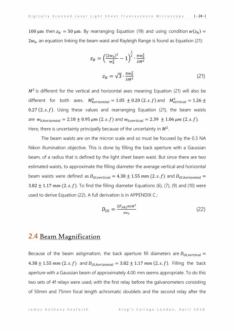
D i g i t a l l y S c a n n e d L a s e r L i g h t S h e e t F l u o r e s c e n c e M i c r o s c o p y | - 26 -|
J a m e s A n t h o n y S e y f o r t h K i n g ’ s C o l l e g e L o n d o n , A p r i l 2 0 1 6
Figure 21: Shows the calculated axial and lateral PSFs for 𝑁𝐴𝑖𝑙𝑙 = 0.105 and 𝑁𝐴𝑑𝑒𝑡 = 0.5 at 𝜆𝑒𝑥𝑐 =
491.5𝑛𝑚, 𝜆𝑒𝑚 = 515𝑛𝑚. 𝐹𝑊𝐻𝑀𝑙𝑎𝑡 = 509 𝑛𝑚 (3. 𝑠. 𝑓) and 𝐹𝑊𝐻𝑀𝑎𝑥 = 2030 𝑛𝑚 (3. 𝑠. 𝑓).
2.6 Digitally Scanned Galvanometers and the Scanning
Angle
The term “Digitally Scanned” is a result of using two computer controlled Galvanometers
to move the light sheet in the x and z axes of the specimen. It is useful to know the
angular deflection 𝛽 of these mirrors as a function of the perpendicular displacement
∆𝑥 from the optical axis in the specimen chamber. This is because the mirrors have a
maximum displacement, i.e. a maximum voltage that can be applied. As a result, the laser
light sheet has a limited total displacement of 2∆𝑥 in the specimen. The equation relating
𝛽 and ∆𝑥 is given by Equation (23), as in [19]:
2𝛽 = 𝑀 ∙ 𝑡𝑎𝑛−1 (∆𝑥
𝑓𝑜𝑏𝑗) (23)
Here 𝑀 is the magnification of the scan lens and tube lens relay and 𝑓𝑜𝑏𝑗 is the focal
length of the illumination of objective. A full derivation and a schematic is found in
APPENDIX D, to provide a full understanding of how the laser light sheet is scanned.
0
0.1
0.2
0.3
0.4
0.5
0.6
0.7
0.8
0.9
1
-3000 -2000 -1000 0 1000 2000 3000
No
rmal
ize
d In
ten
sity
Distance from Center r (nm)
Graph showing the Theoretical Gaussian approximation of the Lateral and Axial PSFs for the DSLM System
lateralresolution,FWHM = 509 nm
axial resolution,FWHM =2030nm
D i g i t a l l y S c a n n e d L a s e r L i g h t S h e e t F l u o r e s c e n c e M i c r o s c o p y | - 27 -|
J a m e s A n t h o n y S e y f o r t h K i n g ’ s C o l l e g e L o n d o n , A p r i l 2 0 1 6
2.7 Piezoelectric Flexure Objective Scanner
To create a 3D volume stack from 2D images it is necessary to move the focal plane of
the objective along the z-axis to match z-position of the light sheet. The method chosen
for this DSLM was to use a piezoelectric linear translator designed exclusively to mount
microscopic objectives. The piezo was a PI-721 PIFOC (PI, 76228 Karlsruhe
Germany) and was operated by applying an input voltage of -2 to +12 Volts which is then
multiplied by 10 by the amplifier. However, the amplifier multiplies the input signal by 10
and the total applied voltage in this investigation was between 0 and 101 Volts. This
corresponded to a displacement of between 0 to 125 micrometres. Further discussion of
the voltage response of the piezo is discussed in section 2.9.
2.8 3D Printed Dual-Objective Lens-Holder
One of the most critical components in the DSLM was custom made and was designed
to hold both the illumination and detection objectives at 90⁰ such that both optical axes
intersect perpendicular to one another. The part was designed using SOLIDWORKS and
printed via Shapeways, the material chosen was a metallic plastic called Alumide, that
consists of nylon and aluminium and is remarkably sturdy, and much cheaper than
printed steel (at $5 per cm3 steel is almost 10 times more expensive to print than Alumide
at $0.56 per cm3). Also, not only is the printing accuracy of the Alumide higher than steel
(± 0.15% compared to ± 5% for steel), the ability to adjust an Alumide component with
low wear during drilling or filing is much more practical than for steel. This was useful
because the tolerance of the printing was not precise enough to accommodate highly
precise optomechanical metal parts, such as posts and screws manufactured by Thorlabs.
The final design was reached via an iterative trial and error process, and
although the first design shown in Figure 22 was effective, it was limited in several ways:
(a) slight inaccuracies were introduced into the post mounting holes due to 3D printing
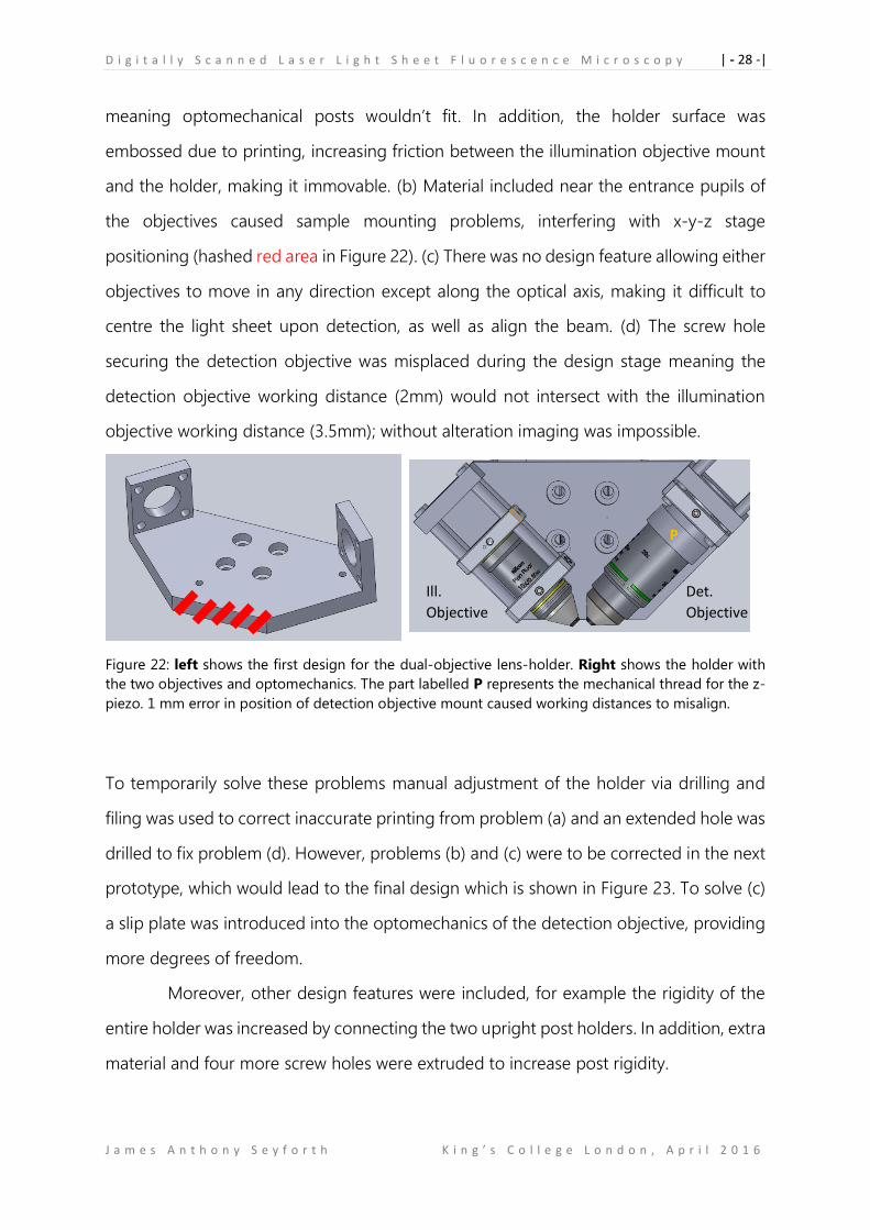
D i g i t a l l y S c a n n e d L a s e r L i g h t S h e e t F l u o r e s c e n c e M i c r o s c o p y | - 28 -|
J a m e s A n t h o n y S e y f o r t h K i n g ’ s C o l l e g e L o n d o n , A p r i l 2 0 1 6
meaning optomechanical posts wouldn’t fit. In addition, the holder surface was
embossed due to printing, increasing friction between the illumination objective mount
and the holder, making it immovable. (b) Material included near the entrance pupils of
the objectives caused sample mounting problems, interfering with x-y-z stage
positioning (hashed red area in Figure 22). (c) There was no design feature allowing either
objectives to move in any direction except along the optical axis, making it difficult to
centre the light sheet upon detection, as well as align the beam. (d) The screw hole
securing the detection objective was misplaced during the design stage meaning the
detection objective working distance (2mm) would not intersect with the illumination
objective working distance (3.5mm); without alteration imaging was impossible.
Figure 22: left shows the first design for the dual-objective lens-holder. Right shows the holder with
the two objectives and optomechanics. The part labelled P represents the mechanical thread for the z-
piezo. 1 mm error in position of detection objective mount caused working distances to misalign.
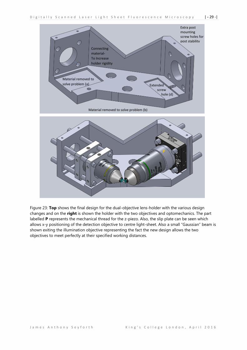
To temporarily solve these problems manual adjustment of the holder via drilling and
filing was used to correct inaccurate printing from problem (a) and an extended hole was
drilled to fix problem (d). However, problems (b) and (c) were to be corrected in the next
prototype, which would lead to the final design which is shown in Figure 23. To solve (c)
a slip plate was introduced into the optomechanics of the detection objective, providing
more degrees of freedom.
Moreover, other design features were included, for example the rigidity of the
entire holder was increased by connecting the two upright post holders. In addition, extra
material and four more screw holes were extruded to increase post rigidity.
Ill.
Objective
Det.
Objective
P
D i g i t a l l y S c a n n e d L a s e r L i g h t S h e e t F l u o r e s c e n c e M i c r o s c o p y | - 29 -|
J a m e s A n t h o n y S e y f o r t h K i n g ’ s C o l l e g e L o n d o n , A p r i l 2 0 1 6
Figure 23: Top shows the final design for the dual-objective lens-holder with the various design
changes and on the right is shown the holder with the two objectives and optomechanics. The part
labelled P represents the mechanical thread for the z-piezo. Also, the slip plate can be seen which
allows x-y positioning of the detection objective to centre light-sheet. Also a small “Gaussian” beam is
shown exiting the illumination objective representing the fact the new design allows the two
objectives to meet perfectly at their specified working distances.
Connecting
material-
To Increase
holder rigidity
Material removed to
solve problem (a) Extended screw hole (d)
Extra post mounting screw holes for post stability
Material removed to solve problem (b)
P
D i g i t a l l y S c a n n e d L a s e r L i g h t S h e e t F l u o r e s c e n c e M i c r o s c o p y | - 30 -|
J a m e s A n t h o n y S e y f o r t h K i n g ’ s C o l l e g e L o n d o n , A p r i l 2 0 1 6
2.8 Fluorescence Detection and Digital Image Acquisition
To detect the emitted sample Fluorescence a Hamamatsu ORCA-ER black and white CCD
Camera was used, which has a resolution of 1.37 Megapixels (1344 pixels x 1024 pixels,
[Width, W] x [Height, H]). Pixels are square with length 6.45 µm. The effective area of the
camera was 8.67 mm [W] x 6.60 mm [H] and the maximum frame rate available in this
investigation, due to software limitation, was 8.3 frames per second.
The pixel size before the entrance of the detection objective is effectively reduced
by the magnification of the 20x Nikon objective, this is because each pixel on the camera
(image plane) must correspond to the same pixel in the sample (object plane), as in [23].
The projected pixel side length was calculated theoretically as 6.45𝜇𝑚
20= 0.323 μ𝑚 (3. 𝑠. 𝑓),
giving a pixel area of 0.104 𝜇𝑚2.
As J. B. Pawley says in [23], “we assume that any microscopic image is just the sum
of the blurred images of the individual “point objects” that make up the object”. He
further discusses that “point objects can be thought of as features smaller than the
smallest details that can be transmitted by the optical system” [23]. Clearly then, if the
resolution of the system is 𝑟𝑙𝑎𝑡 = 0.627μ𝑚 (3. 𝑠. 𝑓) and 𝑟𝑎𝑥 = 2.50 μ𝑚 (3. 𝑠. 𝑓) then the
lateral Airy Disk Diameter will be 𝑑𝑙𝑎𝑡 = 1.25 μ𝑚 (3. 𝑠. 𝑓). To fulfil the Nyquist criterion
“the Airy figure image of a point object should be at least 4 to 5 pixels across the diameter
of its first dark ring”, as in J. B Pawley, [24]. For the lateral resolution in this optical system,
the ideal pixel size would have a side length of between 0.313 μ𝑚 (3. 𝑠. 𝑓) to 0.250 μ𝑚,
calculated using 4 or 5 pixels respectively. Thus, if the estimated pixel size is
0.323 μ𝑚 (3. 𝑠. 𝑓), this corresponds to approximately 3.87 pixels (3. 𝑠. 𝑓) across the Airy
dark ring diameter, meaning that the 20x Objective slightly under-samples and does not
quite meet the Nyquist criterion (But is very close!).
Also important is the illumination of sample features, and in this investigation the
light sheet has values 𝑤0,ℎ𝑜𝑧𝑟𝑖𝑧𝑜𝑛𝑡𝑎𝑙 = 2.18 ± 0.95𝜇𝑚 (2. 𝑠. 𝑓), 𝑤0,𝑣𝑒𝑟𝑡𝑖𝑐𝑎𝑙 = 2.39 ±
1.06𝜇𝑚 (2. 𝑠. 𝑓). J. B. Pawley says in [Figure 4.1, 23] that for illumination, “pixels are one
quarter of the beam diameter”, thus for the smallest estimated beam waist
D i g i t a l l y S c a n n e d L a s e r L i g h t S h e e t F l u o r e s c e n c e M i c r o s c o p y | - 31 -|
J a m e s A n t h o n y S e y f o r t h K i n g ’ s C o l l e g e L o n d o n , A p r i l 2 0 1 6
𝑤0,ℎ𝑜𝑧𝑟𝑖𝑧𝑜𝑛𝑡𝑎𝑙 = 2.18 ± 0.95𝜇𝑚 (2. 𝑠. 𝑓), the ideal pixel size would be 1.09 ±
0.475 μ𝑚 (3. 𝑠. 𝑓). The estimated pixel size is 0.323 μ𝑚 (3. 𝑠. 𝑓), meaning that the
illumination Nyquist criterion is more than satisfied.
Because DSLM produces 4D datasets with 3D spatial image acquisition, the
Nyquist criterion must also be satisfied in the axial dimension. The software used to
control the DSLM was limited to a slice separation of 1μ𝑚 because the LabVIEW software
programmed to control the DSLM was unable to operate at a lower stack separation.
This means that the voxels were rectangular with a depth of 1μ𝑚 and a height/width of
0.323 μ𝑚 (3. 𝑠. 𝑓). Thus, if 𝑑𝑎𝑥 = 5 μ𝑚 (3. 𝑠. 𝑓) then 1μ𝑚 voxel depth is easily satisfying
the Nyquist criterion for the axial dimension.
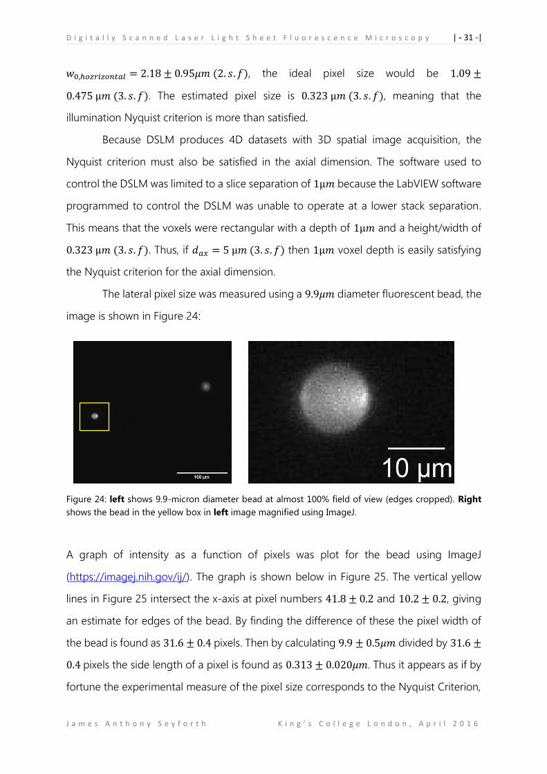
The lateral pixel size was measured using a 9.9𝜇𝑚 diameter fluorescent bead, the
image is shown in Figure 24:
Figure 24: left shows 9.9-micron diameter bead at almost 100% field of view (edges cropped). Right
shows the bead in the yellow box in left image magnified using ImageJ.
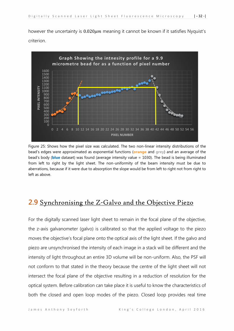
A graph of intensity as a function of pixels was plot for the bead using ImageJ
(https://imagej.nih.gov/ij/). The graph is shown below in Figure 25. The vertical yellow
lines in Figure 25 intersect the x-axis at pixel numbers 41.8 ± 0.2 and 10.2 ± 0.2, giving
an estimate for edges of the bead. By finding the difference of these the pixel width of
the bead is found as 31.6 ± 0.4 pixels. Then by calculating 9.9 ± 0.5𝜇𝑚 divided by 31.6 ±
0.4 pixels the side length of a pixel is found as 0.313 ± 0.020𝜇𝑚. Thus it appears as if by
fortune the experimental measure of the pixel size corresponds to the Nyquist Criterion,
D i g i t a l l y S c a n n e d L a s e r L i g h t S h e e t F l u o r e s c e n c e M i c r o s c o p y | - 32 -|
J a m e s A n t h o n y S e y f o r t h K i n g ’ s C o l l e g e L o n d o n , A p r i l 2 0 1 6
however the uncertainty is 0.020𝜇𝑚 meaning it cannot be known if it satisfies Nyquist’s
criterion.
Figure 25: Shows how the pixel size was calculated. The two non-linear intensity distributions of the
bead’s edges were approximated as exponential functions (orange and grey) and an average of the
bead’s body (blue dataset) was found (average intensity value = 1030). The bead is being illuminated
from left to right by the light sheet. The non-uniformity of the beam intensity must be due to
aberrations, because if it were due to absorption the slope would be from left to right not from right to
left as above.
2.9 Synchronising the Z-Galvo and the Objective Piezo
For the digitally scanned laser light sheet to remain in the focal plane of the objective,
the z-axis galvanometer (galvo) is calibrated so that the applied voltage to the piezo
moves the objective’s focal plane onto the optical axis of the light sheet. If the galvo and
piezo are unsynchronised the intensity of each image in a stack will be different and the
intensity of light throughout an entire 3D volume will be non-uniform. Also, the PSF will
not conform to that stated in the theory because the centre of the light sheet will not
intersect the focal plane of the objective resulting in a reduction of resolution for the
optical system. Before calibration can take place it is useful to know the characteristics of
both the closed and open loop modes of the piezo. Closed loop provides real time
0100200300400500600700800900
1000110012001300140015001600
0 2 4 6 8 10 12 14 16 18 20 22 24 26 28 30 32 34 36 38 40 42 44 46 48 50 52 54 56
PIX
EL IN
TEN
SITY
PIXEL NUMBER
Graph Showing the intnesity profi le for a 9.9 micrometre bead for as a function of pixel number
D i g i t a l l y S c a n n e d L a s e r L i g h t S h e e t F l u o r e s c e n c e M i c r o s c o p y | - 33 -|
J a m e s A n t h o n y S e y f o r t h K i n g ’ s C o l l e g e L o n d o n , A p r i l 2 0 1 6
feedback of the Nano-positioning of the piezo, whereas open loop operates without
feedback. The piezo used was a Physik Instrumente P-721 and had both options available.
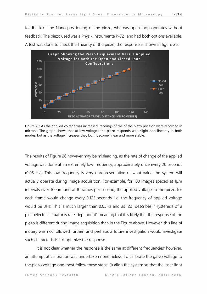
A test was done to check the linearity of the piezo; the response is shown in figure 26:
Figure 26: As the applied voltage was increased, readings of the of the piezo position were recorded in
microns. The graph shows that at low voltages the piezo responds with slight non-linearity in both
modes, but as the voltage increases they both become linear and more stable.
The results of Figure 26 however may be misleading, as the rate of change of the applied
voltage was done at an extremely low frequency, approximately once every 20 seconds
(0.05 Hz). This low frequency is very unrepresentative of what value the system will
actually operate during image acquisition. For example, for 100 images spaced at 1μm
intervals over 100μm and at 8 frames per second, the applied voltage to the piezo for
each frame would change every 0.125 seconds, i.e. the frequency of applied voltage
would be 8Hz. This is much larger than 0.05Hz and as [22] describes, “Hysteresis of a
piezoelectric actuator is rate-dependent” meaning that it is likely that the response of the
piezo is different during image acquisition than in the Figure above. However, this line of
inquiry was not followed further, and perhaps a future investigation would investigate
such characteristics to optimize the response.
It is not clear whether the response is the same at different frequencies; however,
an attempt at calibration was undertaken nonetheless. To calibrate the galvo voltage to
the piezo voltage one most follow these steps: (i) align the system so that the laser light
0
20
40
60
80
100
120
0 20 40 60 80 100 120 140
VO
LTA
GE
V
PIEZO ACTUATOR TRAVEL DISTANCE (MICROMETRES)
Graph Showing the Piezo Displacment Versus Appl ied Voltage for both the Open and Closed Loop
Configurations
closedloopopenloop
D i g i t a l l y S c a n n e d L a s e r L i g h t S h e e t F l u o r e s c e n c e M i c r o s c o p y | - 34 -|
J a m e s A n t h o n y S e y f o r t h K i n g ’ s C o l l e g e L o n d o n , A p r i l 2 0 1 6
y = -0.0024x + 0.1318R² = 0.9967
-0.15
-0.1
-0.05
0
0.05
0.1
0.15
0 20 40 60 80 100 120
GA
LVO
VO
LTA
GE
(V)
PIEZO VOLTAGE (V)
Graph Showing the Galvo Voltage versus Piezo Voltagewith l inear l ine of best fi t
sheet is incident in upon a fluorescently labelled gel and so that the camera is acquiring
an image of the laser light sheet in real time. (ii) now that the piezo is ‘zeroed’, set the
position to its minimum displacement (~0μm) and then manually adjust the
objective/piezo assembly until the laser light sheet is in focus (maximum intensity at
beam waist) (iii) increase the piezo voltage by a desired increment, then adjust the galvo
voltage until the beam is back in focus. Record both voltages. (iv) Repeat step (iii) until
the maximum displacement is reached. (v) Plot the results.
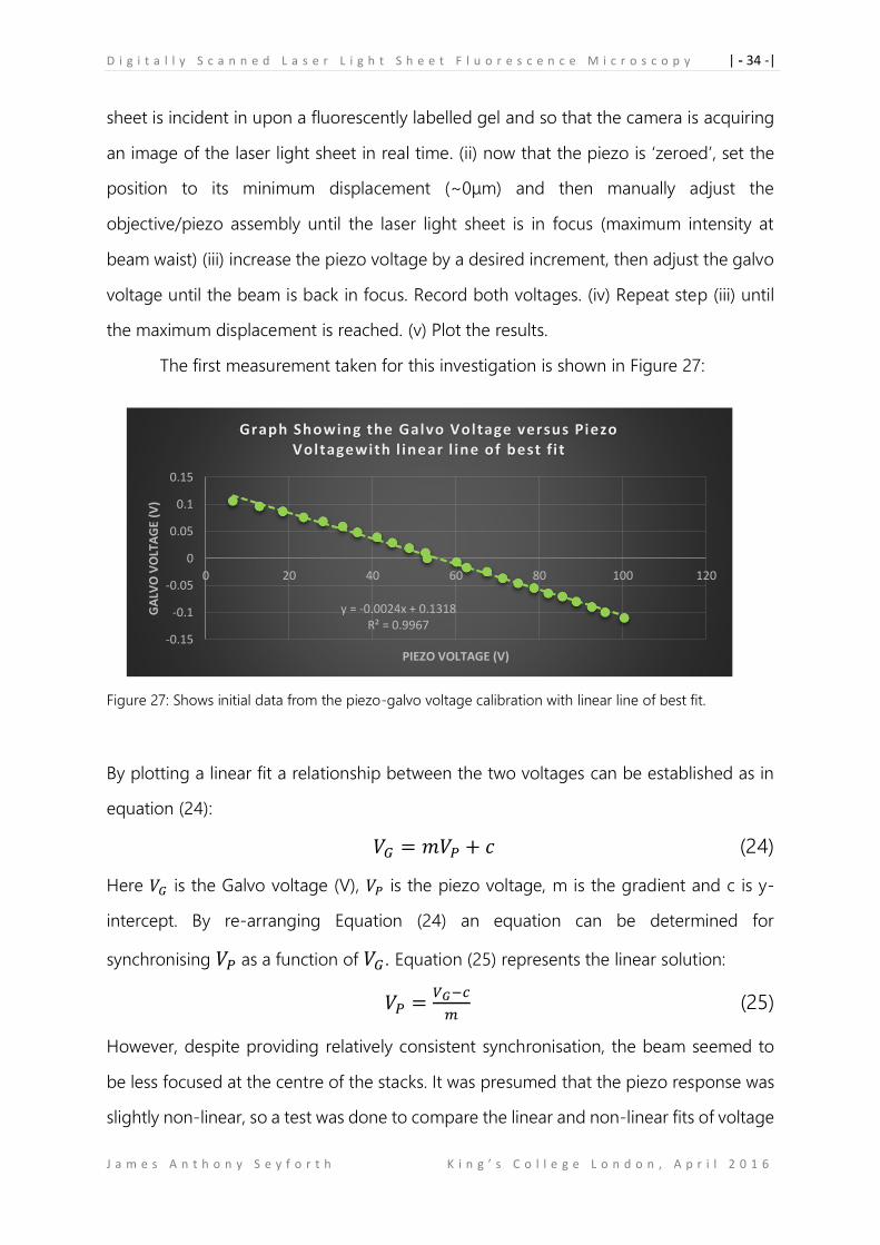
The first measurement taken for this investigation is shown in Figure 27:
Figure 27: Shows initial data from the piezo-galvo voltage calibration with linear line of best fit.
By plotting a linear fit a relationship between the two voltages can be established as in
equation (24):
𝑉𝐺 = 𝑚𝑉𝑃 + 𝑐 (24)
Here 𝑉𝐺 is the Galvo voltage (V), 𝑉𝑃 is the piezo voltage, m is the gradient and c is y-
intercept. By re-arranging Equation (24) an equation can be determined for
synchronising 𝑉𝑃 as a function of 𝑉𝐺. Equation (25) represents the linear solution:
𝑉𝑃 =𝑉𝐺−𝑐
𝑚 (25)
However, despite providing relatively consistent synchronisation, the beam seemed to
be less focused at the centre of the stacks. It was presumed that the piezo response was
slightly non-linear, so a test was done to compare the linear and non-linear fits of voltage
D i g i t a l l y S c a n n e d L a s e r L i g h t S h e e t F l u o r e s c e n c e M i c r o s c o p y | - 35 -|
J a m e s A n t h o n y S e y f o r t h K i n g ’ s C o l l e g e L o n d o n , A p r i l 2 0 1 6
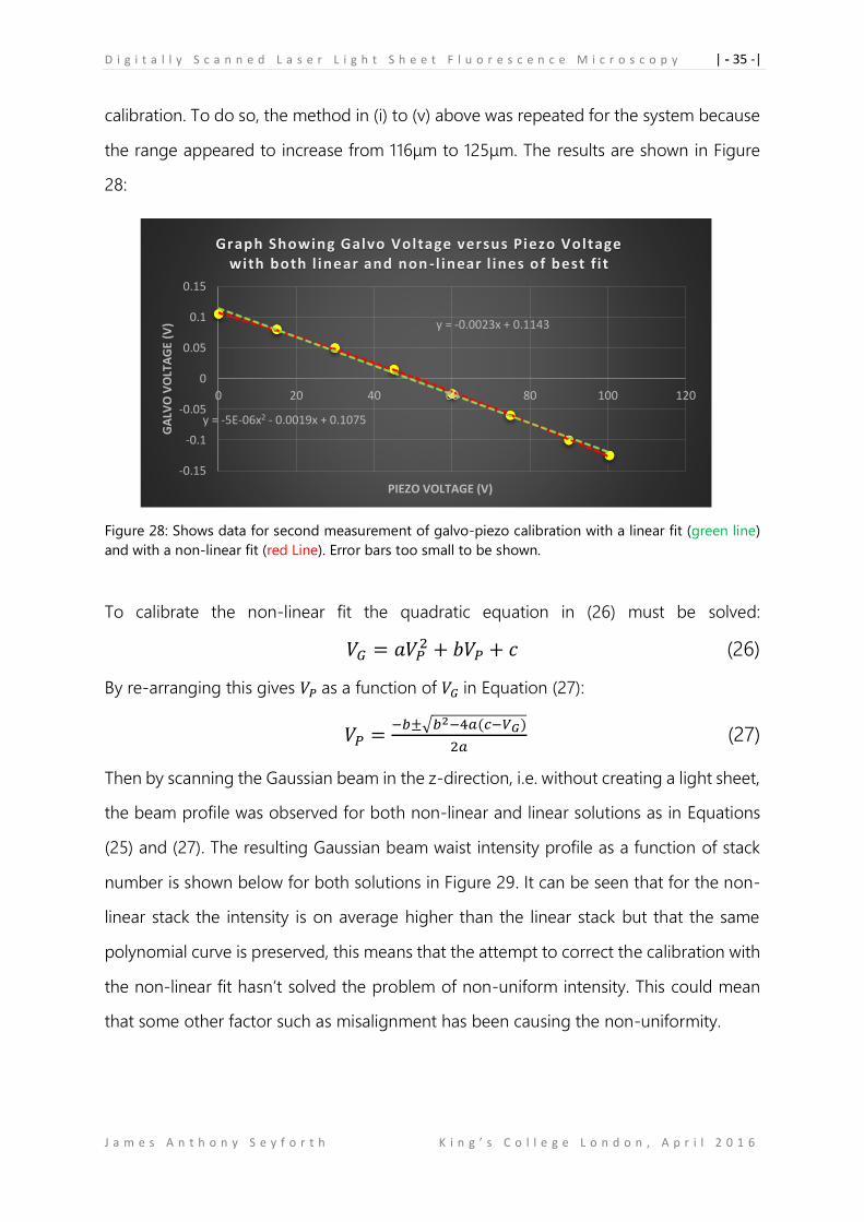
calibration. To do so, the method in (i) to (v) above was repeated for the system because
the range appeared to increase from 116μm to 125μm. The results are shown in Figure
28:
Figure 28: Shows data for second measurement of galvo-piezo calibration with a linear fit (green line)
and with a non-linear fit (red Line). Error bars too small to be shown.
To calibrate the non-linear fit the quadratic equation in (26) must be solved:
𝑉𝐺 = 𝑎𝑉𝑃2 + 𝑏𝑉𝑃 + 𝑐 (26)
By re-arranging this gives 𝑉𝑃 as a function of 𝑉𝐺 in Equation (27):
𝑉𝑃 =−𝑏±√𝑏2−4𝑎(𝑐−𝑉𝐺)
2𝑎 (27)
Then by scanning the Gaussian beam in the z-direction, i.e. without creating a light sheet,
the beam profile was observed for both non-linear and linear solutions as in Equations
(25) and (27). The resulting Gaussian beam waist intensity profile as a function of stack
number is shown below for both solutions in Figure 29. It can be seen that for the non-
linear stack the intensity is on average higher than the linear stack but that the same
polynomial curve is preserved, this means that the attempt to correct the calibration with
the non-linear fit hasn’t solved the problem of non-uniform intensity. This could mean
that some other factor such as misalignment has been causing the non-uniformity.
y = -5E-06x2 - 0.0019x + 0.1075
y = -0.0023x + 0.1143
-0.15
-0.1
-0.05
0
0.05
0.1
0.15
0 20 40 60 80 100 120
GA
LVO
VO
LTA
GE
(V)
PIEZO VOLTAGE (V)
Graph Showing Galvo Voltage versus Piezo Voltage with both l inear and non -l inear l ines of best fi t
D i g i t a l l y S c a n n e d L a s e r L i g h t S h e e t F l u o r e s c e n c e M i c r o s c o p y | - 36 -|
J a m e s A n t h o n y S e y f o r t h K i n g ’ s C o l l e g e L o n d o n , A p r i l 2 0 1 6
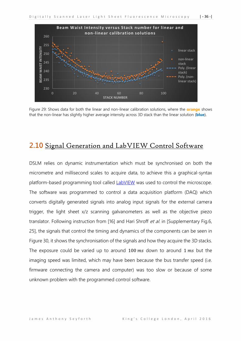
Figure 29: Shows data for both the linear and non-linear calibration solutions, where the orange shows
that the non-linear has slightly higher average intensity across 3D stack than the linear solution (blue).
2.10 Signal Generation and LabVIEW Control Software
DSLM relies on dynamic instrumentation which must be synchronised on both the
micrometre and millisecond scales to acquire data, to achieve this a graphical-syntax
platform-based programming tool called LabVIEW was used to control the microscope.
The software was programmed to control a data acquisition platform (DAQ) which
converts digitally generated signals into analog input signals for the external camera
trigger, the light sheet x/z scanning galvanometers as well as the objective piezo
translator. Following instruction from [16] and Hari Shroff et al. in [Supplementary Fig.6,
25], the signals that control the timing and dynamics of the components can be seen in
Figure 30, it shows the synchronisation of the signals and how they acquire the 3D stacks.
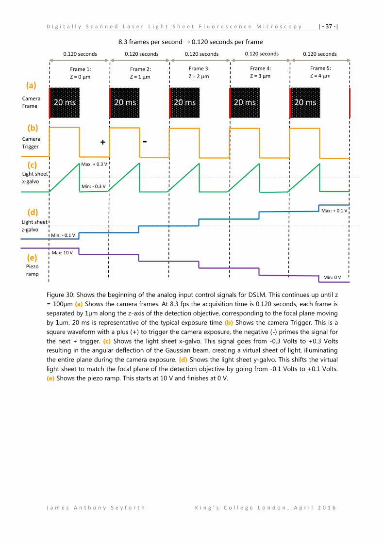
The exposure could be varied up to around 100 𝑚𝑠 down to around 1 𝑚𝑠 but the
imaging speed was limited, which may have been because the bus transfer speed (i.e.
firmware connecting the camera and computer) was too slow or because of some
unknown problem with the programmed control software.
230
235
240
245
250
255
260
0 20 40 60 80 100
BEA
M W
AIS
T IN
TEN
SITY
STACK NUMBER
Beam Waist Intensity versus Stack number for l inear and non-l inear cal ibration solutions
linear stack
non-linearstackPoly. (linearstack)Poly. (non-linear stack)
D i g i t a l l y S c a n n e d L a s e r L i g h t S h e e t F l u o r e s c e n c e M i c r o s c o p y | - 37 -|
J a m e s A n t h o n y S e y f o r t h K i n g ’ s C o l l e g e L o n d o n , A p r i l 2 0 1 6
Figure 30: Shows the beginning of the analog input control signals for DSLM. This continues up until z
= 100µm (a) Shows the camera frames. At 8.3 fps the acquisition time is 0.120 seconds, each frame is
separated by 1µm along the z-axis of the detection objective, corresponding to the focal plane moving
by 1µm. 20 ms is representative of the typical exposure time (b) Shows the camera Trigger. This is a
square waveform with a plus (+) to trigger the camera exposure, the negative (-) primes the signal for
the next + trigger. (c) Shows the light sheet x-galvo. This signal goes from -0.3 Volts to +0.3 Volts
resulting in the angular deflection of the Gaussian beam, creating a virtual sheet of light, illuminating
the entire plane during the camera exposure. (d) Shows the light sheet y-galvo. This shifts the virtual
light sheet to match the focal plane of the detection objective by going from -0.1 Volts to +0.1 Volts.
(e) Shows the piezo ramp. This starts at 10 V and finishes at 0 V.
(c)
Camera
Frame
8.3 frames per second → 0.120 seconds per frame
20 ms 20 ms 20 ms
Frame 1:
Z = 0 µm
Frame 2:
Z = 1 µm
Frame 3:
Z = 2 µm
Frame 4:
Z = 3 µm
Frame 5:
Z = 4 µm
20 ms 20 ms
0.120 seconds 0.120 seconds 0.120 seconds 0.120 seconds 0.120 seconds
Camera
Trigger
Light sheet
x-galvo
Max: + 0.3 V
Min: - 0.3 V
Light sheet
z-galvo
Piezo
ramp
Min: - 0.1 V
Max: + 0.1 V
Max: 10 V
Min: 0 V
+ -
(a)
(b)
(d)
(e)

D i g i t a l l y S c a n n e d L a s e r L i g h t S h e e t F l u o r e s c e n c e M i c r o s c o p y | - 38 -|
J a m e s A n t h o n y S e y f o r t h K i n g ’ s C o l l e g e L o n d o n , A p r i l 2 0 1 6
2.11 Sample Preparation
The first sample was a Fluorescein gel; this was made by combining 1.5% low melting-
point Agarose with the synthetic organic compound Fluorescein, which has an excitation
maximum of ~494nm and an emission maximum ~512nm. This fluorescent gel can be
used to investigate the properties of the light sheet, as it acts as a uniform fluorescent
medium in which the beam propagates.
The mounting of samples is not a trivial problem due to the small working
distances of the water dipping objective lenses (Nikon 10x with 3.5mm WD and Nikon
20x with 2.0mm WD). In addition, if the index of refraction is mismatched between the
lenses and the medium, significant refraction of light can cause spurious results and
aberration, meaning it is crucial to bathe the entrance pupils in pure water. As Huisken
et al discuss in [27], “transparent agarose matches the refractive index of water (1.33) and
biological tissue, and concentrations of 1.0-1.5% provide enough mechanical stability to
reproducibly move the sample”. This means transparent organisms such as foetal
Zebrafish are well matched to agarose and water making for near ideal imaging
conditions. Because of the vertical nature of the microscope a petri dish could be used
as a bath of water. However, because a standard petri dish was used, the sides of the
dish interacted with the objectives meaning the objectives only reached a limited depth
into the dish. A simple and practical way to mount samples, without constructing a
custom mount or using lots of agarose to cover an entire dish bottom, was to sculpt
‘mounds’ of agarose onto a glass coverslip. Figure 31 shows the method used in this
investigation.
The beads were prepared using the same method except that to determine which
dilution was best suited to the region of interest, both 1 in 100 and 1 in 1000 dilutions
were prepared. It was essential to achieve a uniform distribution of beads as well as
ensure that the beads were not clumping together in the agarose. Extensive vortexing
was applied to the bead solution prior to combination with the Agarose; this was
adequate to provide good distribution and separation of the beads.
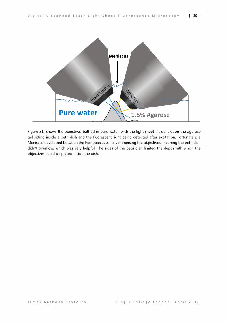
D i g i t a l l y S c a n n e d L a s e r L i g h t S h e e t F l u o r e s c e n c e M i c r o s c o p y | - 39 -|
J a m e s A n t h o n y S e y f o r t h K i n g ’ s C o l l e g e L o n d o n , A p r i l 2 0 1 6
Pure water
Meniscus
1.5% Agarose
Figure 31: Shows the objectives bathed in pure water, with the light sheet incident upon the agarose
gel sitting inside a petri dish and the fluorescent light being detected after excitation. Fortunately, a
Meniscus developed between the two objectives fully immersing the objectives, meaning the petri dish
didn’t overflow, which was very helpful. The sides of the petri dish limited the depth with which the
objectives could be placed inside the dish.
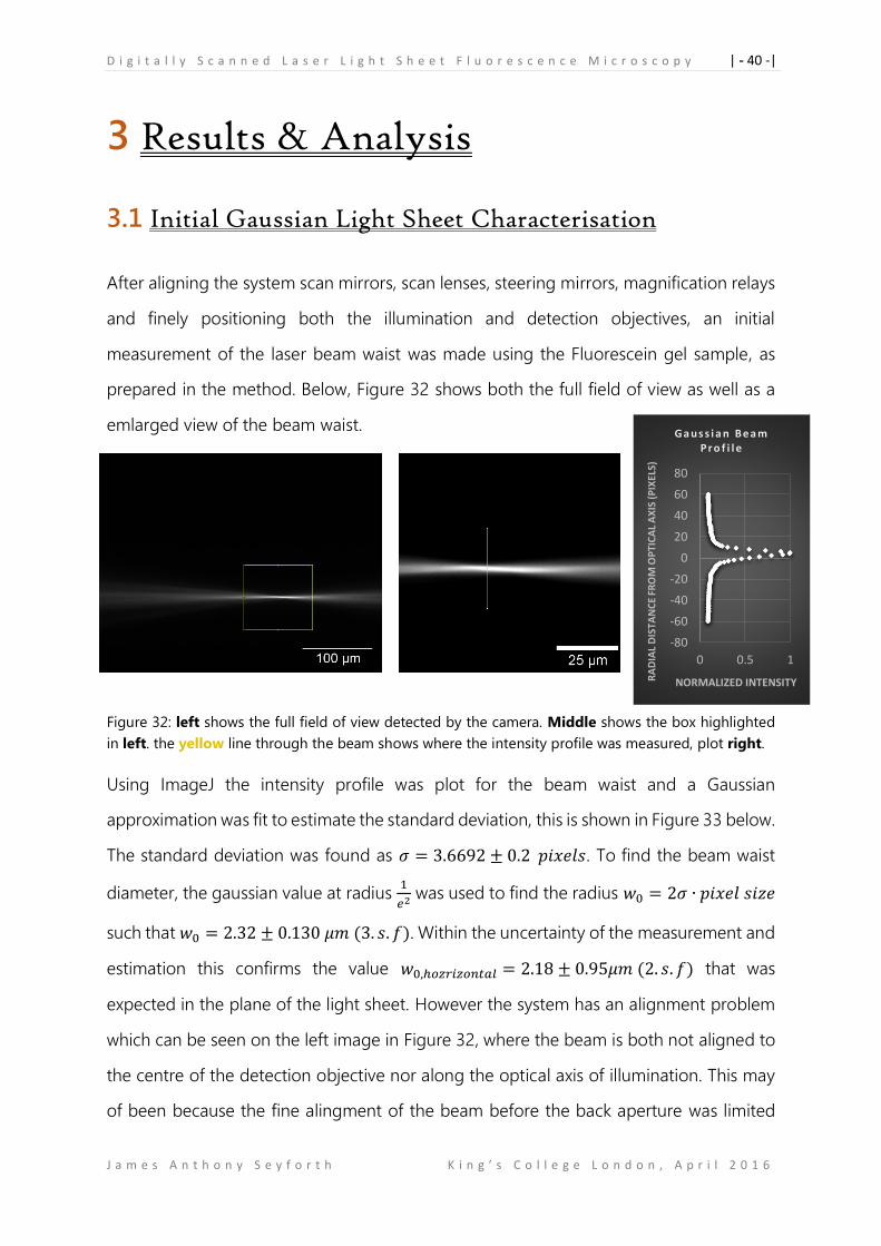
D i g i t a l l y S c a n n e d L a s e r L i g h t S h e e t F l u o r e s c e n c e M i c r o s c o p y | - 40 -|
J a m e s A n t h o n y S e y f o r t h K i n g ’ s C o l l e g e L o n d o n , A p r i l 2 0 1 6
3 Results & Analysis
3.1 Initial Gaussian Light Sheet Characterisation
After aligning the system scan mirrors, scan lenses, steering mirrors, magnification relays
and finely positioning both the illumination and detection objectives, an initial
measurement of the laser beam waist was made using the Fluorescein gel sample, as
prepared in the method. Below, Figure 32 shows both the full field of view as well as a
emlarged view of the beam waist.
Figure 32: left shows the full field of view detected by the camera. Middle shows the box highlighted
in left. the yellow line through the beam shows where the intensity profile was measured, plot right.
Using ImageJ the intensity profile was plot for the beam waist and a Gaussian
approximation was fit to estimate the standard deviation, this is shown in Figure 33 below.
The standard deviation was found as 𝜎 = 3.6692 ± 0.2 𝑝𝑖𝑥𝑒𝑙𝑠. To find the beam waist
diameter, the gaussian value at radius 1
𝑒2 was used to find the radius 𝑤0 = 2𝜎 ∙ 𝑝𝑖𝑥𝑒𝑙 𝑠𝑖𝑧𝑒
such that 𝑤0 = 2.32 ± 0.130 𝜇𝑚 (3. 𝑠. 𝑓). Within the uncertainty of the measurement and
estimation this confirms the value 𝑤0,ℎ𝑜𝑧𝑟𝑖𝑧𝑜𝑛𝑡𝑎𝑙 = 2.18 ± 0.95𝜇𝑚 (2. 𝑠. 𝑓) that was
expected in the plane of the light sheet. However the system has an alignment problem
which can be seen on the left image in Figure 32, where the beam is both not aligned to
the centre of the detection objective nor along the optical axis of illumination. This may
of been because the fine alingment of the beam before the back aperture was limited
-80
-60
-40
-20
0
20
40
60
80
0 0.5 1R
AD
IAL
DIS
TAN
CE
FRO
M O
PTI
CA
L A
XIS
(P
IXE
LS)
NORMALIZED INTENSITY
Ga us s i a n Be a m P r o f i l e
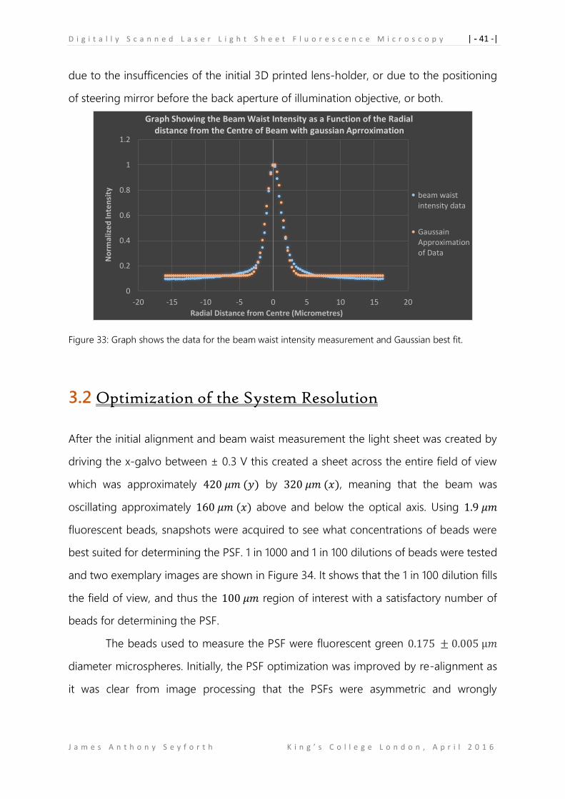
D i g i t a l l y S c a n n e d L a s e r L i g h t S h e e t F l u o r e s c e n c e M i c r o s c o p y | - 41 -|
J a m e s A n t h o n y S e y f o r t h K i n g ’ s C o l l e g e L o n d o n , A p r i l 2 0 1 6
due to the insufficencies of the initial 3D printed lens-holder, or due to the positioning
of steering mirror before the back aperture of illumination objective, or both.
Figure 33: Graph shows the data for the beam waist intensity measurement and Gaussian best fit.
3.2 Optimization of the System Resolution
After the initial alignment and beam waist measurement the light sheet was created by
driving the x-galvo between ± 0.3 V this created a sheet across the entire field of view
which was approximately 420 𝜇𝑚 (𝑦) by 320 𝜇𝑚 (𝑥), meaning that the beam was
oscillating approximately 160 𝜇𝑚 (𝑥) above and below the optical axis. Using 1.9 𝜇𝑚
fluorescent beads, snapshots were acquired to see what concentrations of beads were
best suited for determining the PSF. 1 in 1000 and 1 in 100 dilutions of beads were tested
and two exemplary images are shown in Figure 34. It shows that the 1 in 100 dilution fills
the field of view, and thus the 100 𝜇𝑚 region of interest with a satisfactory number of
beads for determining the PSF.
The beads used to measure the PSF were fluorescent green 0.175 ± 0.005 μ𝑚
diameter microspheres. Initially, the PSF optimization was improved by re-alignment as
it was clear from image processing that the PSFs were asymmetric and wrongly
0
0.2
0.4
0.6
0.8
1
1.2
-20 -15 -10 -5 0 5 10 15 20
No
rmal
ize
d In
ten
sity
Radial Distance from Centre (Micrometres)
Graph Showing the Beam Waist Intensity as a Function of the Radial distance from the Centre of Beam with gaussian Aprroximation
beam waistintensity data
GaussainApproximationof Data
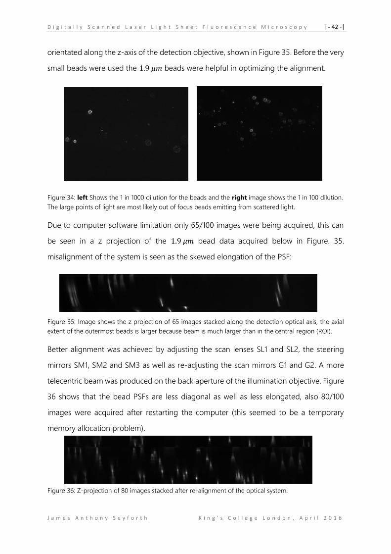
D i g i t a l l y S c a n n e d L a s e r L i g h t S h e e t F l u o r e s c e n c e M i c r o s c o p y | - 42 -|
J a m e s A n t h o n y S e y f o r t h K i n g ’ s C o l l e g e L o n d o n , A p r i l 2 0 1 6
orientated along the z-axis of the detection objective, shown in Figure 35. Before the very
small beads were used the 1.9 𝜇𝑚 beads were helpful in optimizing the alignment.
Figure 34: left Shows the 1 in 1000 dilution for the beads and the right image shows the 1 in 100 dilution.
The large points of light are most likely out of focus beads emitting from scattered light.
Due to computer software limitation only 65/100 images were being acquired, this can
be seen in a z projection of the 1.9 𝜇𝑚 bead data acquired below in Figure. 35.
misalignment of the system is seen as the skewed elongation of the PSF:
Figure 35: Image shows the z projection of 65 images stacked along the detection optical axis, the axial
extent of the outermost beads is larger because beam is much larger than in the central region (ROI).
Better alignment was achieved by adjusting the scan lenses SL1 and SL2, the steering
mirrors SM1, SM2 and SM3 as well as re-adjusting the scan mirrors G1 and G2. A more
telecentric beam was produced on the back aperture of the illumination objective. Figure
36 shows that the bead PSFs are less diagonal as well as less elongated, also 80/100
images were acquired after restarting the computer (this seemed to be a temporary
memory allocation problem).
Figure 36: Z-projection of 80 images stacked after re-alignment of the optical system.
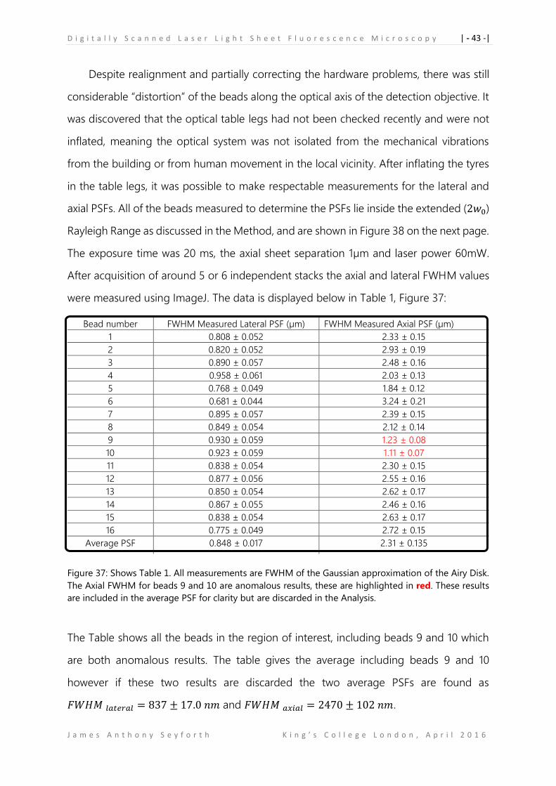
D i g i t a l l y S c a n n e d L a s e r L i g h t S h e e t F l u o r e s c e n c e M i c r o s c o p y | - 43 -|
J a m e s A n t h o n y S e y f o r t h K i n g ’ s C o l l e g e L o n d o n , A p r i l 2 0 1 6
Despite realignment and partially correcting the hardware problems, there was still
considerable “distortion” of the beads along the optical axis of the detection objective. It
was discovered that the optical table legs had not been checked recently and were not
inflated, meaning the optical system was not isolated from the mechanical vibrations
from the building or from human movement in the local vicinity. After inflating the tyres
in the table legs, it was possible to make respectable measurements for the lateral and
axial PSFs. All of the beads measured to determine the PSFs lie inside the extended (2𝑤0)
Rayleigh Range as discussed in the Method, and are shown in Figure 38 on the next page.
The exposure time was 20 ms, the axial sheet separation 1µm and laser power 60mW.
After acquisition of around 5 or 6 independent stacks the axial and lateral FWHM values
were measured using ImageJ. The data is displayed below in Table 1, Figure 37:
Figure 37: Shows Table 1. All measurements are FWHM of the Gaussian approximation of the Airy Disk.
The Axial FWHM for beads 9 and 10 are anomalous results, these are highlighted in red. These results
are included in the average PSF for clarity but are discarded in the Analysis.
The Table shows all the beads in the region of interest, including beads 9 and 10 which
are both anomalous results. The table gives the average including beads 9 and 10
however if these two results are discarded the two average PSFs are found as
𝐹𝑊𝐻𝑀 𝑙𝑎𝑡𝑒𝑟𝑎𝑙 = 837 ± 17.0 𝑛𝑚 and 𝐹𝑊𝐻𝑀 𝑎𝑥𝑖𝑎𝑙 = 2470 ± 102 𝑛𝑚.
Bead number FWHM Measured Lateral PSF (µm) FWHM Measured Axial PSF (µm)
1 0.808 ± 0.052 2.33 ± 0.15
2 0.820 ± 0.052 2.93 ± 0.19
3 0.890 ± 0.057 2.48 ± 0.16
4 0.958 ± 0.061 2.03 ± 0.13
5 0.768 ± 0.049 1.84 ± 0.12
6 0.681 ± 0.044 3.24 ± 0.21
7 0.895 ± 0.057 2.39 ± 0.15
8 0.849 ± 0.054 2.12 ± 0.14
9 0.930 ± 0.059 1.23 ± 0.08
10 0.923 ± 0.059 1.11 ± 0.07
11 0.838 ± 0.054 2.30 ± 0.15
12 0.877 ± 0.056 2.55 ± 0.16
13 0.850 ± 0.054 2.62 ± 0.17
14 0.867 ± 0.055 2.46 ± 0.16
15 0.838 ± 0.054 2.63 ± 0.17
16 0.775 ± 0.049 2.72 ± 0.15
Average PSF 0.848 ± 0.017 2.31 ± 0.135
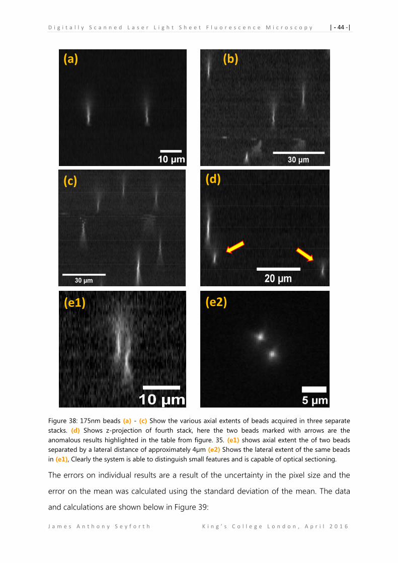
D i g i t a l l y S c a n n e d L a s e r L i g h t S h e e t F l u o r e s c e n c e M i c r o s c o p y | - 44 -|
J a m e s A n t h o n y S e y f o r t h K i n g ’ s C o l l e g e L o n d o n , A p r i l 2 0 1 6
Figure 38: 175nm beads (a) - (c) Show the various axial extents of beads acquired in three separate
stacks. (d) Shows z-projection of fourth stack, here the two beads marked with arrows are the
anomalous results highlighted in the table from figure. 35. (e1) shows axial extent the of two beads
separated by a lateral distance of approximately 4µm (e2) Shows the lateral extent of the same beads
in (e1), Clearly the system is able to distinguish small features and is capable of optical sectioning.
The errors on individual results are a result of the uncertainty in the pixel size and the
error on the mean was calculated using the standard deviation of the mean. The data
and calculations are shown below in Figure 39:
(a) (b)
(c) (d)
(e1) (e2)
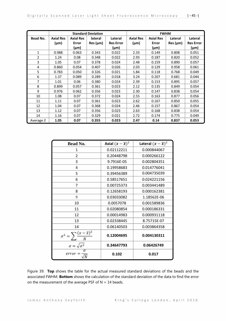
D i g i t a l l y S c a n n e d L a s e r L i g h t S h e e t F l u o r e s c e n c e M i c r o s c o p y | - 45 -|
J a m e s A n t h o n y S e y f o r t h K i n g ’ s C o l l e g e L o n d o n , A p r i l 2 0 1 6
Figure 39: Top shows the table for the actual measured standard deviations of the beads and the
associated FWHM. Bottom shows the calculation of the standard deviation of the data to find the error
on the measurement of the average PSF of N = 14 beads.
Standard Deviation FWHM
Bead No. Axial Res (µm)
Axial Res Error (µm)
lateral Res (µm)
Lateral Res Error
(µm)
Axial Res (µm)
Axial Res Error (µm)
Lateral Res (µm)
Lateral Res Error
(µm)
1 0.988 0.063 0.343 0.022 2.33 0.149 0.808 0.051
2 1.24 0.08 0.348 0.022 2.93 0.187 0.820 0.052
3 1.05 0.07 0.378 0.024 2.48 0.159 0.890 0.057
4 0.860 0.054 0.407 0.026 2.03 0.129 0.958 0.061
5 0.783 0.050 0.326 0.021 1.84 0.118 0.768 0.049
6 1.37 0.089 0.289 0.018 3.24 0.207 0.681 0.044
7 1.01 0.06 0.380 0.024 2.39 0.153 0.895 0.057
8 0.899 0.057 0.361 0.023 2.12 0.135 0.849 0.054
9 0.976 0.062 0.356 0.023 2.30 0.147 0.838 0.054
10 1.08 0.07 0.372 0.024 2.55 0.163 0.877 0.056
11 1.11 0.07 0.361 0.023 2.62 0.167 0.850 0.055
12 1.04 0.07 0.368 0.024 2.46 0.157 0.867 0.054
13 1.12 0.07 0.356 0.023 2.63 0.168 0.838 0.054
14 1.16 0.07 0.329 0.021 2.72 0.174 0.775 0.049
Average �̃� 1.05 0.07 0.355 0.023 2.47 0.14 0.837 0.053
Bead No. Axial (𝒙 − 𝒙)² Lateral (𝒙 − 𝒙)²
1 0.02112211 0.000844067
2 0.20448798 0.000266122
3 9.7916E-05 0.002804351
4 0.19958683 0.014776041
5 0.39456389 0.004735039
6 0.58517651 0.024221156
7 0.00725373 0.003441489
8 0.12658193 0.000162381
9 0.03033082 1.18562E-06
10 0.0057078 0.001589836
11 0.02080854 0.000186331
12 0.00014983 0.000931118
13 0.02338445 8.75715E-07
14 0.06140503 0.003864358
𝜎2 = ∑(𝑥 − �̃�)2
𝑁 0.12004695 0.004130311
𝜎 = √𝜎2 0.34647793 0.06426749
𝑒𝑟𝑟𝑜𝑟 =𝜎
√𝑁 0.102 0.017
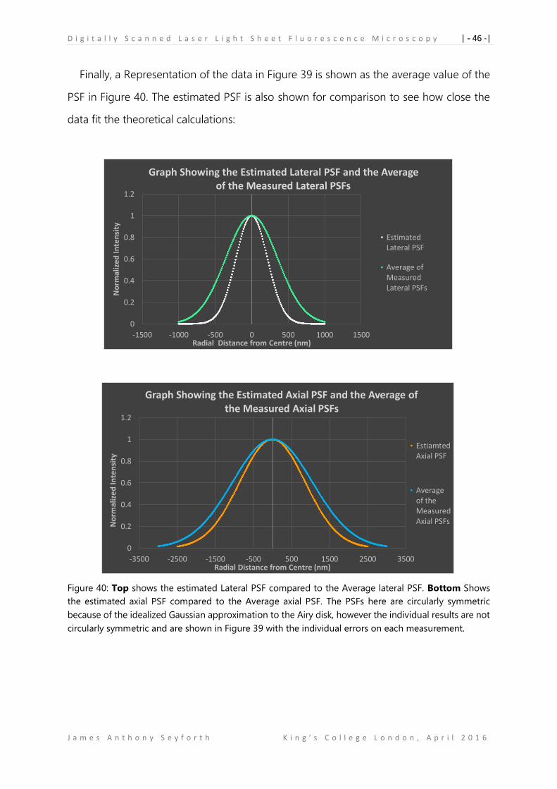
D i g i t a l l y S c a n n e d L a s e r L i g h t S h e e t F l u o r e s c e n c e M i c r o s c o p y | - 46 -|
J a m e s A n t h o n y S e y f o r t h K i n g ’ s C o l l e g e L o n d o n , A p r i l 2 0 1 6
Finally, a Representation of the data in Figure 39 is shown as the average value of the
PSF in Figure 40. The estimated PSF is also shown for comparison to see how close the
data fit the theoretical calculations:
Figure 40: Top shows the estimated Lateral PSF compared to the Average lateral PSF. Bottom Shows
the estimated axial PSF compared to the Average axial PSF. The PSFs here are circularly symmetric
because of the idealized Gaussian approximation to the Airy disk, however the individual results are not
circularly symmetric and are shown in Figure 39 with the individual errors on each measurement.
0
0.2
0.4
0.6
0.8
1
1.2
-1500 -1000 -500 0 500 1000 1500
No
rmal
ize
d In
ten
sity
Radial Distance from Centre (nm)
Graph Showing the Estimated Lateral PSF and the Average of the Measured Lateral PSFs
EstimatedLateral PSF
Average ofMeasuredLateral PSFs
0
0.2
0.4
0.6
0.8
1
1.2
-3500 -2500 -1500 -500 500 1500 2500 3500
No
rmal
ize
d In
ten
sity
Radial Distance from Centre (nm)
Graph Showing the Estimated Axial PSF and the Average of the Measured Axial PSFs
EstiamtedAxial PSF
Averageof theMeasuredAxial PSFs
D i g i t a l l y S c a n n e d L a s e r L i g h t S h e e t F l u o r e s c e n c e M i c r o s c o p y | - 47 -|
J a m e s A n t h o n y S e y f o r t h K i n g ’ s C o l l e g e L o n d o n , A p r i l 2 0 1 6
3.3 Discussion of Results
The average PSFs were measured as 𝐹𝑊𝐻𝑀 𝑙𝑎𝑡𝑒𝑟𝑎𝑙 = 837 ± 17.0 𝑛𝑚 and 𝐹𝑊𝐻𝑀 𝑎𝑥𝑖𝑎𝑙 =
2470 ± 102 𝑛𝑚, these can be compared to the estimated PSFs which were 𝐹𝑊𝐻𝑀𝑙𝑎𝑡 =
509𝑛𝑚 (3. 𝑠. 𝑓) and 𝐹𝑊𝐻𝑀𝑎𝑥 = 2030 𝑛𝑚 (3. 𝑠. 𝑓). Both measurements are larger than
the expected PSFs and do not fall within the measurement uncertainty indicating there
was a systematic error causing the mismatch.
The discrepancy above will be discussed further below, however it is useful to
compare the results found during this investigation to other scanning, as well as non-
scanning SPIM devices, to assess the quality of the measurements. For example, in an
investigation by Wu, Li and Chan in [28] they showed that by using 10x illumination and
48x detection objectives, they could achieve an average 𝐹𝑊𝐻𝑀 𝑙𝑎𝑡𝑒𝑟𝑎𝑙 = 810 ± 70 𝑛𝑚
and 𝐹𝑊𝐻𝑀 𝑎𝑥𝑖𝑎𝑙 = 1420 ± 150 𝑛𝑚. The lateral resolution they measured is close to that
of this investigation, but the axial resolution is much better. However, Wu et al. imaged
phytoplankton, where a “flow sheath is used to hydro-dynamically focus particles into
the central part of a square capillary” [28]. If the method of estimating the resolution is
used as in [15] and this experiment, Wu et al. should have expected an approximate
𝐹𝑊𝐻𝑀 𝑙𝑎𝑡𝑒𝑟𝑎𝑙 = 297 𝑛𝑚 and 𝐹𝑊𝐻𝑀 𝑎𝑥𝑖𝑎𝑙 = 945 𝑛𝑚 at laser excitation at 450𝑛𝑚. But,
even with no laminar flow of phytoplankton, the glass capillary, which has both a sheath
and a core, could cause “severe aberrations” as discussed in [27] and also in [5]. Thus,
these results may not as useful as other scanning light sheet microscopes in assessing
the merit of the measurements presented above.
Furthermore, In the diSPIM protocol in [26], which utilises dual illumination and
detection, Shroff et al. describe in supplementary table 4 that for each detection arm they
are achieving approximately a 𝐹𝑊𝐻𝑀 𝑙𝑎𝑡𝑒𝑟𝑎𝑙 = 500 ± 20 𝑛𝑚 and 𝐹𝑊𝐻𝑀 𝑎𝑥𝑖𝑎𝑙 = 1700 ±
150 𝑛𝑚 before deconvolution. Their device utilises two 40x 0.8NA Nikon water-dipping
objectives for illumination and detection; interestingly they avoid mounting in agarose
and describe how “embedding a sample in agarose is cumbersome for a large variety of
specimens that are more easily grown or deposited on conventional glass coverslips”,
D i g i t a l l y S c a n n e d L a s e r L i g h t S h e e t F l u o r e s c e n c e M i c r o s c o p y | - 48 -|
J a m e s A n t h o n y S e y f o r t h K i n g ’ s C o l l e g e L o n d o n , A p r i l 2 0 1 6
[26]. However, their device is more relevant to this analysis because they didn’t use a
glass capillary. The higher lateral resolution found for their device reflects the fact that
both illumination and detection were at 0.8 NA giving more flexibility over the Gaussian
light sheet as well as significant increase in light gathering capabilities. Also the error in
their lateral measurement is 0.04%, which is closer to that found in this investigation
(0.02%) than in [28], which is 0.08%.
Also, the results measured for this DSLM show that the axial resolution is ~2.95x
greater than the lateral resolution; Shroff et al. find theirs at ~3.4x, whereas Wu et al.
finds ~1.75x. This indicates that Shroff et al. are achieving the best resolution because
they are closest to Stelzers’s claim that SPIM can achieve a high lateral resolution and
maintain an axial resolution only four times greater [15]. Wu et al. acknowledge that the
shadowing artefacts they found as well as the lower lateral resolution they achieved
“could be overcome by illuminating the sample from opposite sides” [28]. Moreover, as
discussed in Figures. 27-30 in [5], the depth of imaging and the concentration of Agarose
have significant effects on the quality of the resolution, this is because: (1) The light has
to travel through more agarose to reach deeper beads causing scattering and
astigmatism and (2) The beads themselves are subject to forces that cause them to drift,
causing distortions in time-lapse imaging [5]. The agarose used for the measurements in
this DSLM was 1.5% agarose which is considerably stable, but unfortunately the imaging
depth was highly variable and can only be quantified as approximately 0 − 2000𝜇𝑚,
which could have caused serious scattering and distorted both the axial and lateral PSF
measurements. In addition, the ‘mound’ of agarose used to hold the beads was an
arbitrary shape with irregular curved edges that must have contributed more
unquantified aberrations. Also, some of the beads seemed to have distortions along the
axial extent, this may have been caused by the drift or it may have been caused by the
vibrations of the x-galvo and piezo as they returned from maximum to minimum Voltage
causing a disturbance in the medium.
Another scanning device is an IsoView light sheet microscope, developed by P. J.
Keller et al. as in [29] uses twice as many views as in [26] two create a four view digitally
D i g i t a l l y S c a n n e d L a s e r L i g h t S h e e t F l u o r e s c e n c e M i c r o s c o p y | - 49 -|
J a m e s A n t h o n y S e y f o r t h K i n g ’ s C o l l e g e L o n d o n , A p r i l 2 0 1 6
scanning microscope that can image at an axial and lateral resolution of 420 ±
20 𝜇𝑚 after Multiview deconvolution. However, each arm images at 600 ±
30 𝜇𝑚 (𝑙𝑎𝑡𝑒𝑟𝑎𝑙𝑙𝑦) and 2980 ± 290 𝜇𝑚 (𝑎𝑥𝑖𝑎𝑙𝑙𝑦) [29]. This is a remarkable increase in
isotopic resolution and is demonstrative of the power of Light sheet microscopy to
resolve images in 3D as well as 4D. They use custom made 0.714 NA microscopic
objectives designed to fit within the geometry constraints of four closely spaced
objectives all moving in synchrony to illuminate and detect light via scanning and
translating.
Many devices, including those in [5], [26] and [29] show that the isotropic resolution
can be greatly increased by acquiring multiple views, whether that be by rotating the
sample or by placing more optics about the specimen chamber. This approach will be
considered for a future DSLM, but not only because it will increase the resolution but
because it also solves the problem of imaging at depth in samples, as discussed by Kržič
in [5]. Kržič describes that when using Multiview imaging, a “blurred and dimmed region
in one view is replaced by the information from a complimentary view, where this region
is sharper and brighter”, [5].
Another limitation of this microscope is that the calibration of the y-galvanometer
and the objective piezo was not demonstrating perfect synchronisation, perhaps due to
rate dependent hysteresis of the piezo, or bad alignment. This caused some images in
each stack to be illuminated by the beam waist and others illuminated by light either side
of the waist. This would need to be corrected in the future to achieve optimal resolution,
otherwise when combined with scattering inside an actual biological sample, the device
will struggle to optically section such organisms because the contrast will be heavily
reduced in the centre of the specimen.
Also, time was lost towards the end of the investigation due to hard disk corruption
on the laboratory computer, as well as a hazardous leak in the lab from the floor above.
This meant that the possibility of gathering 4D data on a live zebrafish was not possible
before the submission of this project report.
D i g i t a l l y S c a n n e d L a s e r L i g h t S h e e t F l u o r e s c e n c e M i c r o s c o p y | - 50 -|
J a m e s A n t h o n y S e y f o r t h K i n g ’ s C o l l e g e L o n d o n , A p r i l 2 0 1 6
The beam itself was elliptical before entering the illumination objective and should
be ‘circularized’ for future investigations, as the beam artefacts could have been causing
problems with the quality of the light sheet as well as the symmetry of the beam as
discussed in the method. To do so, one would have to place a pinhole after the first set
of relay lenses, this would remove the beam ‘wing’ causing the problem, creating a “more
visually circular” beam in the near-field as discussed is [30]. This is fine because the beam
used in this DSLM travels very short distances between each component of the system
and never really reaches the far-field where it will become elliptical again. Also, “a small
circular aperture can cause power loss as high as 80% and strong far field diffraction
rings” as in [30]. The power to excite the fluorescent beads is roughly 60mw and the laser
is rated as up to 200mw. It would be possible to limit power loss at 60% meaning even If
imaging at 200mw with a circular aperture, 80mw would still be; more than enough
power to excite fluorescence, [30].
One interesting study by T. Vettenburg et al. in [31] shows a comparison between
Gaussian, Bessel and Airy beam illumination, where the Bessel beam can be tuned “to
the percentage ratio β = w/R = 0.10 and 0.05, respectively” using a spatial light modulator
(SLM). The β = 0.10 beam extends the field of view two-fold compared to the Gaussian
beam, whereas the β = 0.05 beam extends the field of view three-fold, but decreases
contrast and resolution. However, by using an Airy beam they manage to increase the
field of view 10-fold whilst maintaining an even higher resolution than the Gaussian beam.
Although the Airy beam is better, a two-photon Bessel beam is still very useful
considering the small ROI in this experiment, and the method demonstrated by Betzig et
al. in [16] is more than adequate and would be a significant upgrade on the Gaussian
beam.
D i g i t a l l y S c a n n e d L a s e r L i g h t S h e e t F l u o r e s c e n c e M i c r o s c o p y | - 51 -|
J a m e s A n t h o n y S e y f o r t h K i n g ’ s C o l l e g e L o n d o n , A p r i l 2 0 1 6
3.4 Conclusions
In conclusion, this investigation has realized a high resolution Digitally Scanned Laser
Light Sheet Fluorescence Microscope, as well as documented the fundamental principles
by which it operates and can be controlled. The system resolution was estimated to be
𝐹𝑊𝐻𝑀𝑙𝑎𝑡 = 509𝑛𝑚 (3. 𝑠. 𝑓) and 𝐹𝑊𝐻𝑀𝑎𝑥 = 2030 𝑛𝑚 (3. 𝑠. 𝑓) and using green
fluorescent beads the actual average PSFs were measured as 𝐹𝑊𝐻𝑀 𝑙𝑎𝑡𝑒𝑟𝑎𝑙 = 837 ±
17.0 𝑛𝑚 and 𝐹𝑊𝐻𝑀 𝑎𝑥𝑖𝑎𝑙 = 2470 ± 102 𝑛𝑚. The estimates matched the values given by
Stelzer et al. in [15] and the measurements were comparable in quality to the
measurements found by Shroff et al. in [26].
As described in [5], [26] and [28] the deviation in the measured PSFs from the
estimates was most likely because of the depth of which the beads were imaged in the
Agarose. Moreover, the astigmatic beam could have been the cause of both the
asymmetry in the laser light sheet as well alignment issues, resulting in decreased spatial
resolution; this could be fixed by using a pinhole to “circularize” the beam. In addition,
the calibration of the piezo could be optimized to ensure a uniform intensity of light
across the entire field of view as well as across the entire depth of view. To correct this,
research into rate dependent hysteresis may be necessary to improve synchronisation
between the piezo and y-galvanometer. Unfortunately, problems with the computer and
lab stalled the acquisition of 4D data on zebrafish, however a new computer is being
installed with higher memory and processing power which should make controlling the
DSLM more reliable.
Finally, an upgraded DSLM would utilise Multiview imaging with deconvolution to
increase isotropic resolution and decrease shadowing [32]. Furthermore, by including a
two-photon Bessel beam, the field of view would increase at least two-fold and also
increase the contrast, resolution and optical sectioning capability.
D i g i t a l l y S c a n n e d L a s e r L i g h t S h e e t F l u o r e s c e n c e M i c r o s c o p y | - 52 -|
J a m e s A n t h o n y S e y f o r t h K i n g ’ s C o l l e g e L o n d o n , A p r i l 2 0 1 6
Acknowledgments
This project would not have been possible were not for the exceptional support and
encouragement of my Supervisor Dr Simon Ameer-Beg, as well as the members of the
Ameer-Beg Research group. In particular, thank you to Dr Simon Poland who’s
experience with LabVIEW and instrument control was invaluable to this investigation.
Also, I would to thank those of the Knight Group from the Craniofacial Development and
Stem Cell Biology Division for providing support with sample preparation. In particular,
thank you to Dr Claire Mitchell.
Many thanks to the Physics department for providing me with the opportunity to
collaborate with the Randall Division of Cell & Molecular Biophysics, and thank you to
the latter for providing the research space to construct the DSLM.
Finally, thank you to all my family and friends for continually inspiring and supporting me
through all my endeavours.
D i g i t a l l y S c a n n e d L a s e r L i g h t S h e e t F l u o r e s c e n c e M i c r o s c o p y | - 53 -|
J a m e s A n t h o n y S e y f o r t h K i n g ’ s C o l l e g e L o n d o n , A p r i l 2 0 1 6
References
[1] Periklis Pantazis and Willy Supatto, “Advances in whole-embryo imaging: a
quantitative transition is underway”, Nature Reviews,, Molecular Cell Biology, Volume
15, May 2014, pages 327 – 339
[2] Ernst H. K. Stelzer, Christoph Cremer and Steffen Lindek, “Theory and Applications of Confocal
Theta Microscopy”, Zoological Studies 34, Supplement 1 (1995), Proceedings of Focus on
Microscopy ‚95 , Pages 67-69
[3] Emmanuel G. Reynaud, Uroš Kržič, Klaus Greger and Ernst H.K. Stelzer, “Light sheet-based
fluorescence microscopy: more dimensions, more photons, and less photodamage”, HFSP J.
2008 Oct; 2(5): pages 266–275., doi: 10.2976/1.2974980
[4] Philipp J. Keller, Annette D. Schmidt, Joachim Wittbrodt and Ernst H.K. Stelzer,
“Reconstruction of Zebrafish Early Embryonic Development by Scanned Light Sheet
Microscopy”, Science 322, 1065 (2008); pages 1065-1069, DOI: 10.1126/science.1162493
[5] Uroš Kržič, “Multiple-view microscopy with light-sheet based fluorescence
microscope”, Dissertation submitted to the combined faculties for the natural Sciences
and for Mathematics of the Ruperto-Carola University of Heidelberg, Germany for the
degree of Doctor of Natural Sciences, http://www.ub.uni-heidelberg.de/archiv/9668
[6] Florian O. Fahrbach, Fabian F. Voigt, Benjamin Schmid, Fritjof Helmchen, and Jan
Huisken, “Rapid 3D light-sheet microscopy with a tuneable lens”, Optics Express Vol.
21, Issue 18, pp. 21010-21026 (2013)
[7] Li Li, Bo Yan, Yu-Qian Shi, Wen-Qing Zhang and Zi-Long Wen, “Live Imaging Reveals
Differing Roles of Macrophages and Neutrophils during Zebrafish Tail Fin
Regeneration” J Biol Chem. 2012 Jul 20; 287(30): 25353–25360. Published online 2012
May 9. doi: 10.1074/jbc.M112.349126
[8] Hecht E. (2002) “optics (4th edition)”, published in San Francisco, Pearson Education.,
publishing as Addison Wesley.
[9] Siegman A. E. (1986) “LASERS”, published: Sausalito, CA by University Science Books
[10] Sidney A. Self, “Focusing of spherical Gaussian beams”, Applied Optics, Vol. 22, No. 5,
1 March 1983, pages 658-661
[11] Ariel Lipson, Stephen G. Lipson, Henry Lipson, 2011, “Optical Physics (4th Edition)”,
Published in USA by Cambridge University Press page 51
[12] Michael W. Davidson and Mortimer Abramowitz, (2002) “OPTICAL MICROSCOPY”
Published online by John Wiley & Sons, Inc.
D i g i t a l l y S c a n n e d L a s e r L i g h t S h e e t F l u o r e s c e n c e M i c r o s c o p y | - 54 -|
J a m e s A n t h o n y S e y f o r t h K i n g ’ s C o l l e g e L o n d o n , A p r i l 2 0 1 6
[13] Mortimer Abramowitz, Kenneth R. Spring, H. Ernst Keller, and Michael W. Davidson,
“Basic Principles of Microscope Objectives”, Biotechniques, bioimaging, Vol. 33, No. 4
(2002)
[14] Editor James B. Pawley, (2006), “Handbook of Biological Confocal Microscopy (3rd
Edition)”, published in New York by Springer Science + Business,
[15] Christoph J. Engelbrecht and Ernst H. K. Stelzer, “Resolution enhancement in a light-
sheet-based microscope (SPIM)”, May 15, 2006 / Vol. 31, No. 10 / OPTICS LETTERS,
pages 1477-1479
[16] Liang Gao, Lin Shao, Bi-Chang Chen & Eric Betzig, “3D live fluorescence imaging of
cellular dynamics using Bessel beam plane illumination microscopy”, Nature America,
NATURE PROTOCOLS VOL.9 NO.5 2014 pages 1083-1101
[17] Abbe, E.(1873) “Beiträge zur Theorie des Mikroskops und der mikroskopischen
Wahrnehmung”, Arch. f. Microsc. Anat. 9:413.
[18] Pitrone PG, Schindelin J, Stuyvenberg L, Preibisch S, Weber M, Eliceiri KW, Huisken
J, Tomancak P., “OpenSPIM: an open-access light-sheet microscopy platform”, Nat
Methods. 2013 Jul;10(7):598-9. doi: 10.1038/nmeth.2507. Epub 2013 Jun 9.
[19] Ernst H.K. Stelzer, “The Intermediate Optical System of Laser-Scanning Confocal
Microscopes”, Handbook of Biological Confocal Microscopy, Third Edition, edited by
James B. Pawley, Springer Science + Business Media, LLC, New York, 2006.
[20] Professor A. E. Siegman, “How to (Maybe) Measure Laser Beam Quality” Diode
Pumped Solid State Lasers: Applications and Issues 1998, Washington D.C., United
States1 January 1998, ISBN: 1-55752-520-X
[21] © The Author(s) 2015 H. Sun, “A Practical Guide to Handling Laser Diode Beams”,
Springer Briefs in Physics, DOI 10.1007/978-94-017-9783-2_2
[22] Wei Tech Ang, Francisco Alija Garmón, Pradeep K. Khosla, and Cameron N. Riviere,
“Modeling Rate-dependent Hysteresis in Piezoelectric Actuator”, The Robotics
Institute, Carnegie Mellon University, Pittsburgh, PA 15213, USA
[23] James B. Pawley, “Points, Pixels and Gray Levels: Digitizing Image Data”, Handbook of
Biological Confocal Microscopy, Third Edition, edited by James B. Pawley, Springer
Science + Business Media, LLC, New York, 2006.
[24] James B. Pawley, “Fundamental limits in Confocal Microscopy”, Handbook of Biological
Confocal Microscopy, Third Edition, edited by James B. Pawley, Springer Science +
Business Media, LLC, New York, 2006.
D i g i t a l l y S c a n n e d L a s e r L i g h t S h e e t F l u o r e s c e n c e M i c r o s c o p y | - 55 -|
J a m e s A n t h o n y S e y f o r t h K i n g ’ s C o l l e g e L o n d o n , A p r i l 2 0 1 6
[25] Yicong Wu, Peter Wawrzusin, Justin Senseney, Robert S Fischer, Ryan Christensen,
Anthony Santella, Andrew G York, Peter W Winter, Clare M Waterman, Zhirong Bao,
Daniel A Colón-Ramos, Matthew McAuliffe & Hari Shroff, “Spatially isotropic four-
dimensional imaging with dual-view plane illumination microscopy”, Nature Biotechnology
31, 1032–1038 (2013) doi:10.1038/nbt.2713
[26] Abhishek Kumar, Yicong Wu, Ryan Christensen, Panagiotis Chandris, William Gandler,
Evan McCreedy, Alexandra Bokinsky, Daniel A Colón-Ramos, Zhirong Bao, Matthew
McAuliffe, Gary Rondeau & Hari Shroff, “Dual-view plane illumination microscopy for
rapid and spatially isotropic imaging”, Nature Protocols, VoL.9 No.11, 2014, pages
2555-2573
[27] Anna Kaufmann, Michaela Mickoleit, Michael Weber and Jan Huisken, “Multilayer
mounting enables long-term imaging of zebrafish development in a light sheet
microscope”, Development 139, 3242-3247 (2012) doi:10.1242/dev.082586 © 2012.
Published by The Company of Biologists Ltd
[28] Jianglai Wu, Jianping Li and Robert K.Y. Chan, “A light sheet based high throughput
3D-imaging flow cytometer for phytoplankton analysis”, 17 June 2013, Vol. 21, No. 12,
Optics Express 14474
[29] Raghav K Chhetri, Fernando Amat, Yinan Wan, Burkhard Höckendorf, William C Lemon
& Philipp J Keller, “Whole-animal functional and developmental imaging with isotropic
spatial resolution”, Nature Methods 12, pages 1171–1178 (2015)
[30] “LASER DIODE TECHNICAL NOTE 1: Beam Circularization and Astigmatism-correction”
Coherent Auburn Group Laser Diode Module EUROPE Coherent GmbH Dieselstraße
5b D-64807 Dieburg, Germany
[31] Tom Vettenburg, Heather I C Dalgarno, Jonathan Nylk, Clara Coll-Lladó, David E K
Ferrier, Tomáš Čižmár, Frank J Gunn-Moore & Kishan Dholakia, “Light sheet
microscopy using an Airy beam”, Nature Methods, 11, Pages 541–544 (2014)
[32] Francesco Pampaloni , Bo-Jui Chang, Ernst H. K. Stelzer, “Light sheet-based
fluorescence microscopy (LSFM) for the quantitative imaging of cells and
tissues”, Cell and Tissue Research, April 2015, Volume 360, Issue 1, pp 129-141
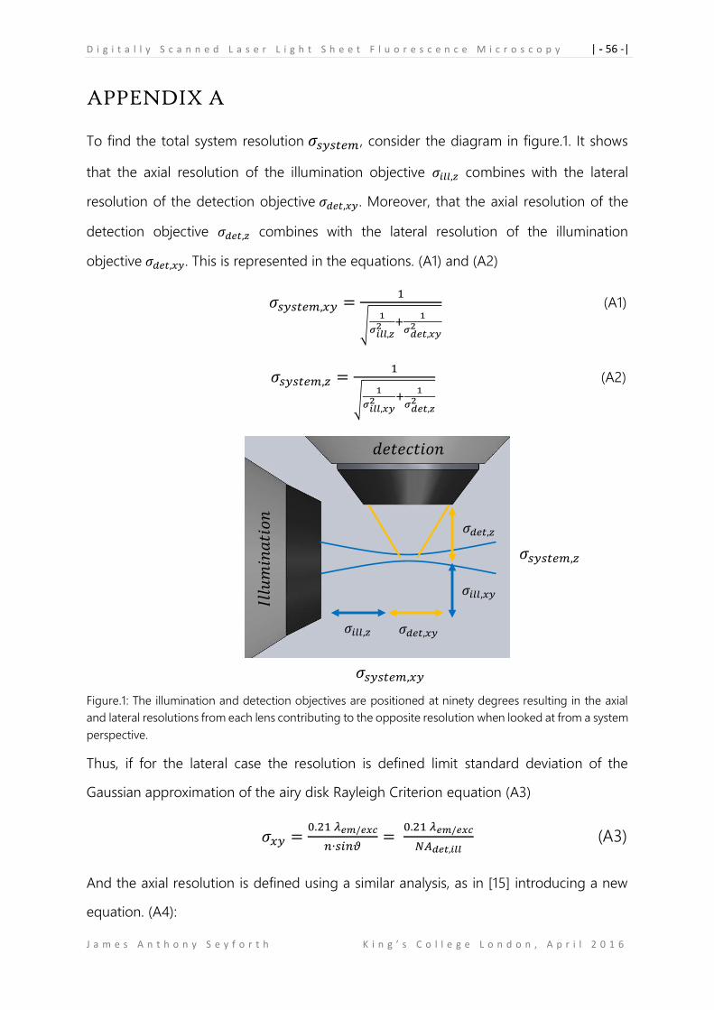
D i g i t a l l y S c a n n e d L a s e r L i g h t S h e e t F l u o r e s c e n c e M i c r o s c o p y | - 56 -|
J a m e s A n t h o n y S e y f o r t h K i n g ’ s C o l l e g e L o n d o n , A p r i l 2 0 1 6
APPENDIX A
To find the total system resolution 𝜎𝑠𝑦𝑠𝑡𝑒𝑚 , consider the diagram in figure.1. It shows
that the axial resolution of the illumination objective 𝜎𝑖𝑙𝑙,𝑧 combines with the lateral
resolution of the detection objective 𝜎𝑑𝑒𝑡,𝑥𝑦. Moreover, that the axial resolution of the
detection objective 𝜎𝑑𝑒𝑡,𝑧 combines with the lateral resolution of the illumination
objective 𝜎𝑑𝑒𝑡,𝑥𝑦. This is represented in the equations. (A1) and (A2)
𝜎𝑠𝑦𝑠𝑡𝑒𝑚,𝑥𝑦 =1
√1
𝜎𝑖𝑙𝑙,𝑧2 +
1
𝜎𝑑𝑒𝑡,𝑥𝑦2
(A1)
𝜎𝑠𝑦𝑠𝑡𝑒𝑚,𝑧 =1
√1
𝜎𝑖𝑙𝑙,𝑥𝑦2 +
1
𝜎𝑑𝑒𝑡,𝑧2
(A2)
Figure.1: The illumination and detection objectives are positioned at ninety degrees resulting in the axial
and lateral resolutions from each lens contributing to the opposite resolution when looked at from a system
perspective.
Thus, if for the lateral case the resolution is defined limit standard deviation of the
Gaussian approximation of the airy disk Rayleigh Criterion equation (A3)
𝜎𝑥𝑦 =0.21 𝜆𝑒𝑚/𝑒𝑥𝑐
𝑛∙𝑠𝑖𝑛𝜗=
0.21 𝜆𝑒𝑚/𝑒𝑥𝑐
𝑁𝐴𝑑𝑒𝑡,𝑖𝑙𝑙 (A3)
And the axial resolution is defined using a similar analysis, as in [15] introducing a new
equation. (A4):
𝜎𝑠𝑦𝑠𝑡𝑒𝑚,𝑧
𝜎𝑠𝑦𝑠𝑡𝑒𝑚,𝑥𝑦
𝜎𝑖𝑙𝑙,𝑧
𝜎𝑑𝑒𝑡,𝑥𝑦
𝜎𝑑𝑒𝑡,𝑧
𝜎𝑖𝑙𝑙,𝑥𝑦
𝐼𝑙𝑙𝑢
𝑚𝑖𝑛
𝑎𝑡𝑖
𝑜𝑛
𝑑𝑒𝑡𝑒𝑐𝑡𝑖𝑜𝑛
D i g i t a l l y S c a n n e d L a s e r L i g h t S h e e t F l u o r e s c e n c e M i c r o s c o p y | - 57 -|
J a m e s A n t h o n y S e y f o r t h K i n g ’ s C o l l e g e L o n d o n , A p r i l 2 0 1 6
𝜎𝑧 =0.34𝜆𝑒𝑚/𝑒𝑥𝑐
𝑛(1−cos(𝜗𝑑𝑒𝑡,𝑖𝑙𝑙)) (A4)
Looking at equation. (A4), it can be seen that low value NA objectives will give a low
value of angular aperture 𝜗, this will give large values of 𝜎𝑧. Because DLSM uses low NA
illumination optics, 𝜎𝑖𝑙𝑙,𝑧 for DLSM will be large. Because 𝜎𝑖𝑙𝑙,𝑧 is much larger, 𝜎2𝑖𝑙𝑙,𝑧 will
also be much greater and so the term 1
𝜎𝑖𝑙𝑙,𝑥𝑦2 will be considerably smaller than
1
𝜎𝑑𝑒𝑡,𝑧2 in
equation (4B) meaning the system resolution tends to be determined only by 𝜎𝑖𝑙𝑙,𝑧. This
results in equation 4B becoming:
𝜎𝑠𝑦𝑠𝑡𝑒𝑚,𝑥𝑦 =1
√1
𝜎𝑑𝑒𝑡,𝑧2
And so:
𝜎𝑠𝑦𝑠𝑡𝑒𝑚,𝑥𝑦 =1
√(0.21𝜆𝑒𝑚
𝑁𝐴𝑑𝑒𝑡)
2=
0.21𝜆𝑒𝑚
𝑁𝐴𝑑𝑒𝑡
But since the two resolutions for 𝜎𝑠𝑦𝑠𝑡𝑒𝑚,𝑥𝑦 are comparable thus equation (4A) leads to:
𝜎𝑠𝑦𝑠𝑡𝑒𝑚,𝑧 =1
√1
𝜎𝑖𝑙𝑙,𝑥𝑦2 +
1
𝜎𝑑𝑒𝑡,𝑧2
𝜎𝑠𝑦𝑠𝑡𝑒𝑚,𝑧 =1
√(1
0.21𝜆𝑒𝑥𝑐𝑁𝐴𝑖𝑙𝑙
)
2
+(1
0.34𝜆𝑒𝑚𝑛(1−cos(𝜗𝑑𝑒𝑡))
)
2
=1
√(𝑁𝐴𝑖𝑙𝑙
0.21𝜆𝑒𝑥𝑐)
2+(
𝑛(1−cos(𝜗𝑑𝑒𝑡))
0.34𝜆𝑒𝑚)
2= ((
𝑁𝐴𝑖𝑙𝑙
0.21𝜆𝑒𝑥𝑐)
2
+ (𝑛(1−cos(𝜗𝑑𝑒𝑡))
0.34𝜆𝑒𝑚)
2)
−1
2
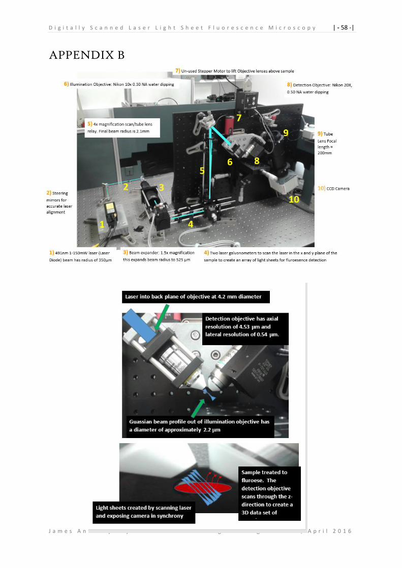
D i g i t a l l y S c a n n e d L a s e r L i g h t S h e e t F l u o r e s c e n c e M i c r o s c o p y | - 58 -|
J a m e s A n t h o n y S e y f o r t h K i n g ’ s C o l l e g e L o n d o n , A p r i l 2 0 1 6
APPENDIX B

D i g i t a l l y S c a n n e d L a s e r L i g h t S h e e t F l u o r e s c e n c e M i c r o s c o p y | - 59 -|
J a m e s A n t h o n y S e y f o r t h K i n g ’ s C o l l e g e L o n d o n , A p r i l 2 0 1 6
APPENDIX C
To find the Gaussian beam radius that must fill the microscope objectives back aperture
equations (C1), (C2), (C3), and (C4) were must be used:
𝜃 = 𝑡𝑎𝑛−1 (𝑤(𝑧)
𝑧) (C1)
𝑁𝐴 = 𝑛 ∙ sin (𝜗) (C2)
𝑀𝑎𝑔𝑛𝑖𝑓𝑖𝑐𝑎𝑡𝑖𝑜𝑛 =𝑓𝑜𝑐𝑎𝑙 𝑙𝑒𝑛𝑔𝑡ℎ 𝑜𝑓 𝑡𝑢𝑏𝑒 𝑙𝑒𝑛𝑠
𝑓𝑜𝑐𝑎𝑙 𝑙𝑒𝑛𝑔𝑡ℎ 𝑜𝑓 𝐼𝑛𝑓𝑖𝑛𝑖𝑡𝑦 𝑜𝑏𝑗𝑒𝑐𝑡𝑖𝑣𝑒 (C3)
𝐷𝑓𝑖𝑛𝑎𝑙 = 2𝐹𝑜𝑏𝑗𝑁𝐴 (C4)
In the limit as 𝑧 → ∞ Gaussian far field divergence half angle is approximated as 𝜃 ≈
𝜆𝑀2
𝜋𝑤0 from (C1). Then, by equating this angle with the angular aperture of the objective 𝜗
from (C2) the numerical aperture is given as:
𝑁𝐴 = 𝑛 ∙ sin (𝜆𝑀2
𝜋𝑤0
)
In the near field at the microscopic beam waist, the angle 𝜃 ≪ 1, using sin(𝜃) ≈ 𝜃 the
NA becomes:
𝑁𝐴 = 𝑛 ∙𝜆𝑀2
𝜋𝑤0
Using (C4) and inserting the above equation for the numerical aperture, the diameter of
the Gaussian beam on the back aperture is given by:
𝐷𝑖𝑙𝑙 =2𝐹𝑜𝑏𝑗𝑛𝜆𝑀2
𝜋𝑤0
D i g i t a l l y S c a n n e d L a s e r L i g h t S h e e t F l u o r e s c e n c e M i c r o s c o p y | - 60 -|
J a m e s A n t h o n y S e y f o r t h K i n g ’ s C o l l e g e L o n d o n , A p r i l 2 0 1 6
APPENDIX D
To find the vertical light sheet displacement Δ𝑥 as a function of scanning mirror angle 𝛽,
it is necessary to consider the arguments set forth in [19] for telecentric lenses (in this
case an objective lens with entrance pupil imaged at infinity. Also, two other fundamental
geometrical optics arguments must be put forward: (A) For a light beam incident upon a
mirror tilted at an angle 𝛽, the angle of reflection is 2𝛽. And (B) that the angular
magnification for a telescopic lens arrangement is given by (D1):
𝑀𝑎𝑛𝑔𝑢𝑙𝑎𝑟 =𝑎𝑛𝑔𝑙𝑒 𝜃1 𝑏𝑒𝑓𝑜𝑟𝑒 𝑓1
𝑎𝑛𝑔𝑙𝑒 𝜃2 𝑎𝑓𝑡𝑒𝑟 𝑓2=
𝑓2
𝑓1 (D1)
For the scanning mirrors, tube lens and infinity corrected illumination objective set up
used in this investigation, 𝑓1 = 50𝑚𝑚, 𝑓2 = 200𝑚, and from so 𝑀 = 4. If the mirror is
tilted by 𝛽 then the beam angle must be 𝜃1 = 2𝛽 from condition (A) meaning 𝜃2 =2𝛽
4=
𝛽
2. This arrangement can be seen in Figure. 1:
Figure. 1: Shows the telecentric objective with scan lens and tube lens. The tube lens must be 200mm from
the illumination objective (IO) otherwise the beam will not be stationary on the back focal plane of the IO,
meaning the light sheet will have unwanted angular displacement from the optical axis.
Thus to find the displacement of the light sheet after the illumination objective front
aperture a second diagram must be drawn for the objective, as in figure. 2:
𝛽
2𝛽 𝛽
2
𝑓1 = 50𝑚𝑚 𝑓2 = 200𝑚𝑚
𝜃1 𝜃2
𝑆𝑐𝑎𝑛 𝑙𝑒𝑛𝑠
𝑇𝑢𝑏𝑒 𝑙𝑒𝑛𝑠
𝐼𝑙𝑙𝑢𝑚𝑖𝑛𝑎𝑡𝑖𝑜𝑛 𝑜𝑏𝑗𝑒𝑐𝑡𝑖𝑣𝑒
D i g i t a l l y S c a n n e d L a s e r L i g h t S h e e t F l u o r e s c e n c e M i c r o s c o p y | - 61 -|
J a m e s A n t h o n y S e y f o r t h K i n g ’ s C o l l e g e L o n d o n , A p r i l 2 0 1 6
Δ𝑥
Figure. 2: Two beams enter the objective at angle 𝜃2, this means that after exiting the
front aperture the angular aperture of the two focused beams will also be 𝜃2.
Thus is it can be seen from ray tracing, and using elementary trigonometry that (D2) as
in [19]:
tan(𝜃2) =∆𝑥
𝑓𝑜𝑏𝑗 (D2)
Thus if we want to find the total field of view below and above optical axis after the
aperture (i.e. in sample),first we compute it as a function of 𝜃1:
tan(𝜃2) =∆𝑥
𝑓𝑜𝑏𝑗
Which becomes:
tan (𝜃1
𝑀) =
∆𝑥
𝑓𝑜𝑏𝑗
Therefore:
𝜃1 = 𝑀 ∙ 𝑡𝑎𝑛−1 (∆𝑥
𝑓𝑜𝑏𝑗)
So for this DSLM the angular displacement from the optical axis at the mirror must be
𝛽 =𝑀
2∙ 𝑡𝑎𝑛−1 (
∆𝑥
𝑓𝑜𝑏𝑗)
But the total angular displacement to create a light sheet is twice this:
2𝛽 = 𝑀 ∙ 𝑡𝑎𝑛−1 (∆𝑥
𝑓𝑜𝑏𝑗)