Embed Size (px)
Citation preview
Real-Time Rendering
Digital Image SynthesisYung-Yu Chuang01/03/2006
with slides by Ravi Ramamoorthi and Robin Green
Realistic rendering
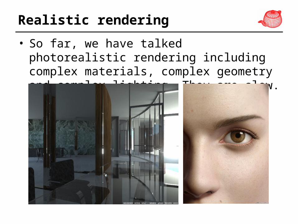
• So far, we have talked photorealistic rendering including complex materials, complex geometry and complex lighting. They are slow.
Real-time rendering
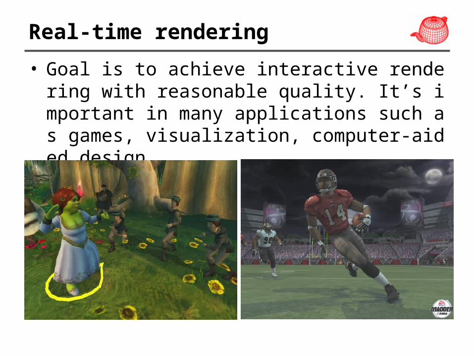
• Goal is to achieve interactive rendering with reasonable quality. It’s important in many applications such as games, visualization, computer-aided design, …
Basic themes
• Interactive ray-tracing• Programmable graphics hardware• Image-based rendering• Precomputation-based methods
Natural illumination
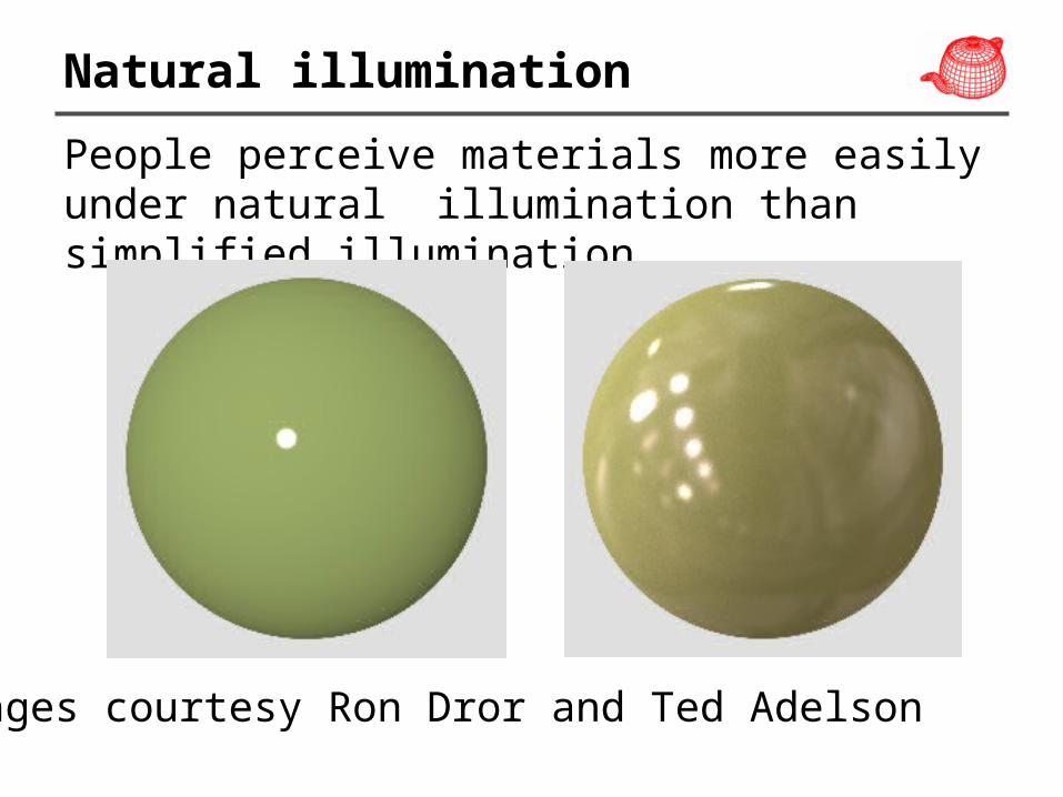
People perceive materials more easily under natural illumination than simplified illumination.
Images courtesy Ron Dror and Ted Adelson
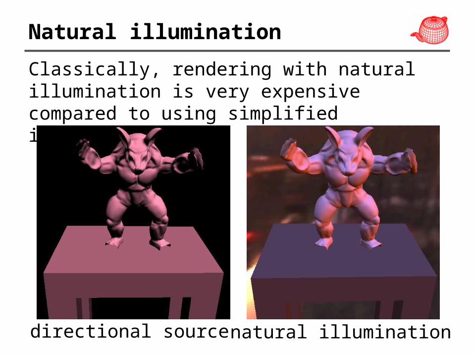
Natural illumination
Classically, rendering with natural illumination is very expensive compared to using simplified illumination
directional source natural illumination
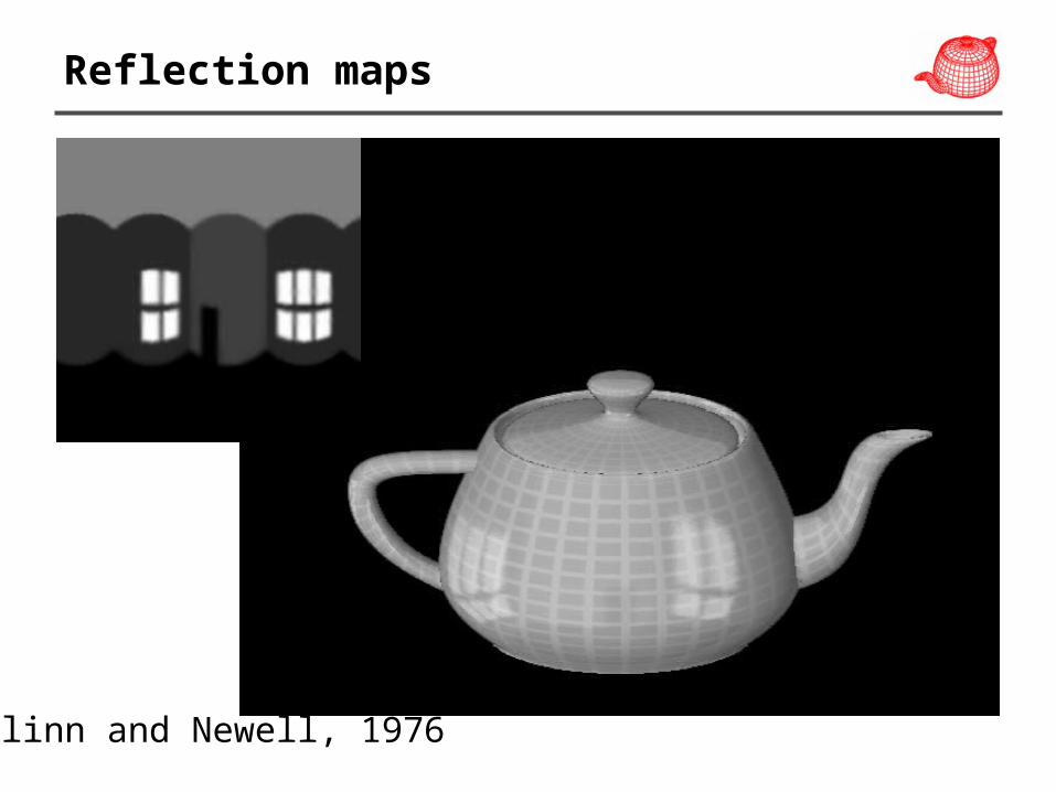
Reflection maps
Blinn and Newell, 1976
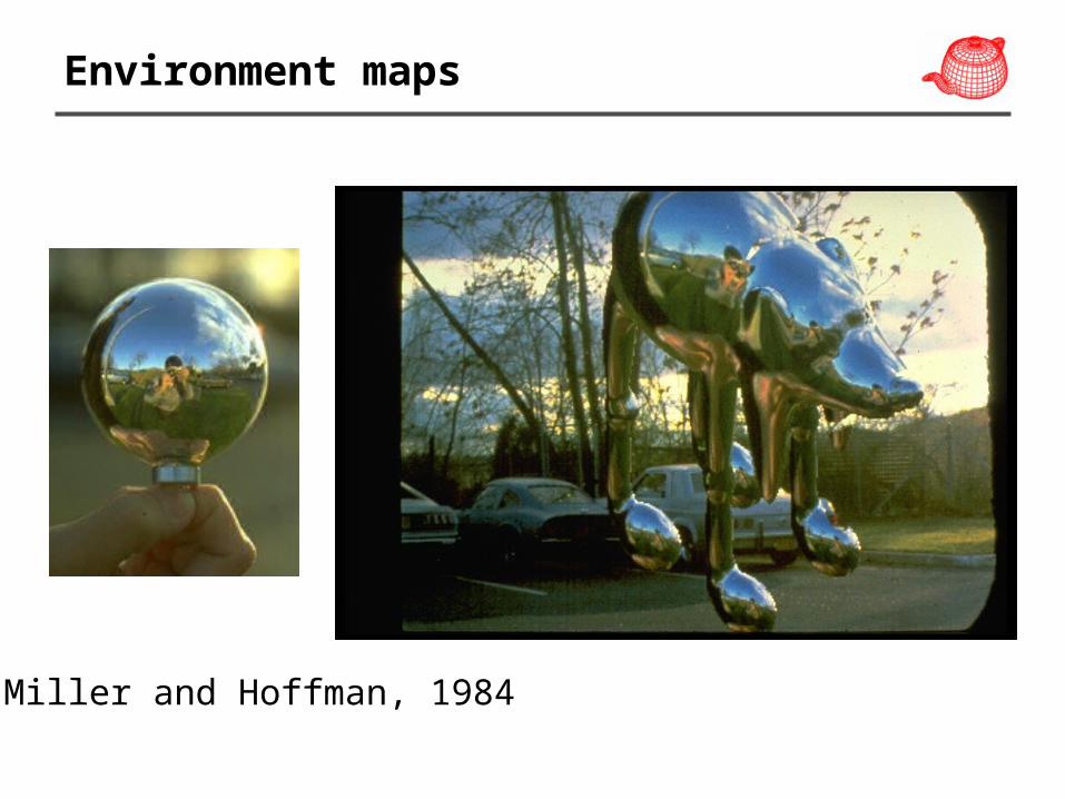
Environment maps
Miller and Hoffman, 1984
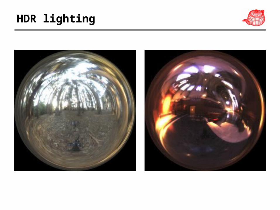
HDR lighting
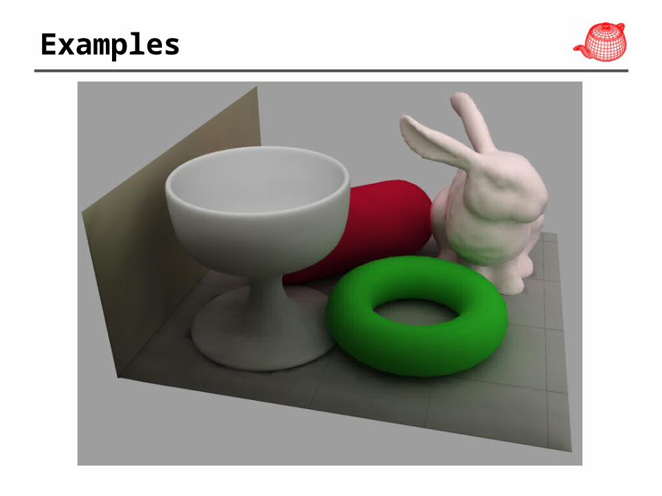
Examples
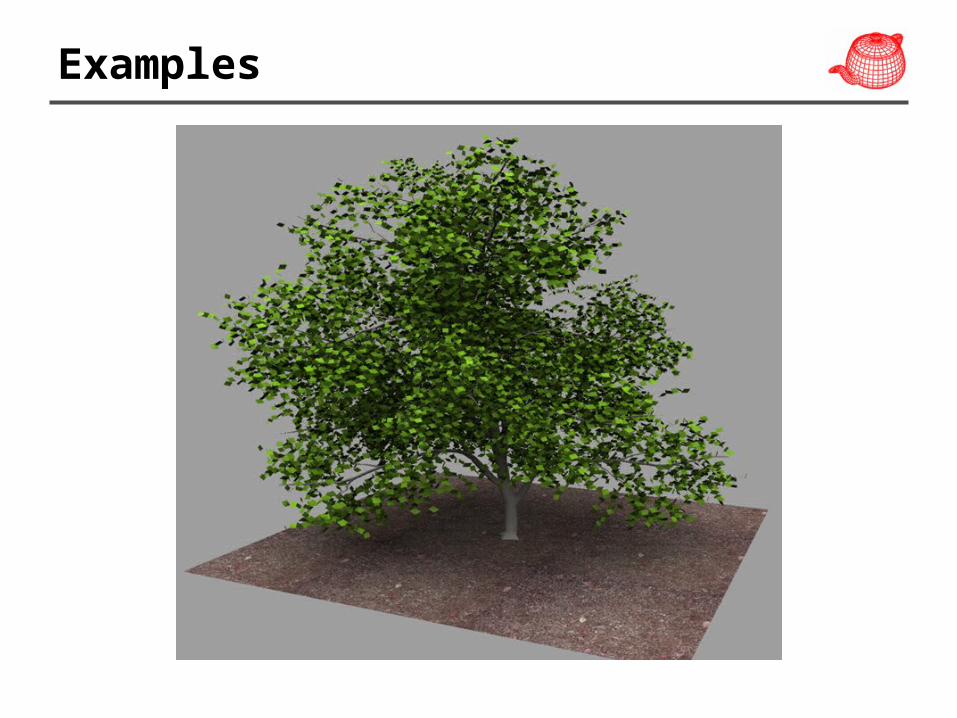
Examples
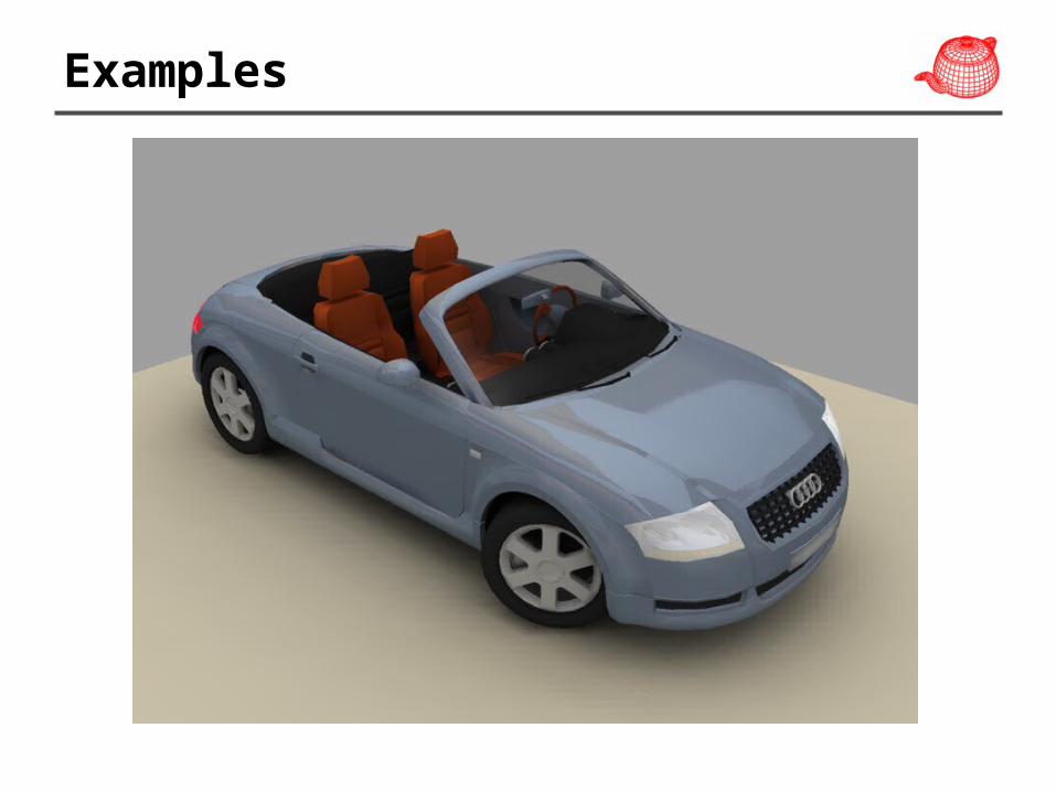
Examples
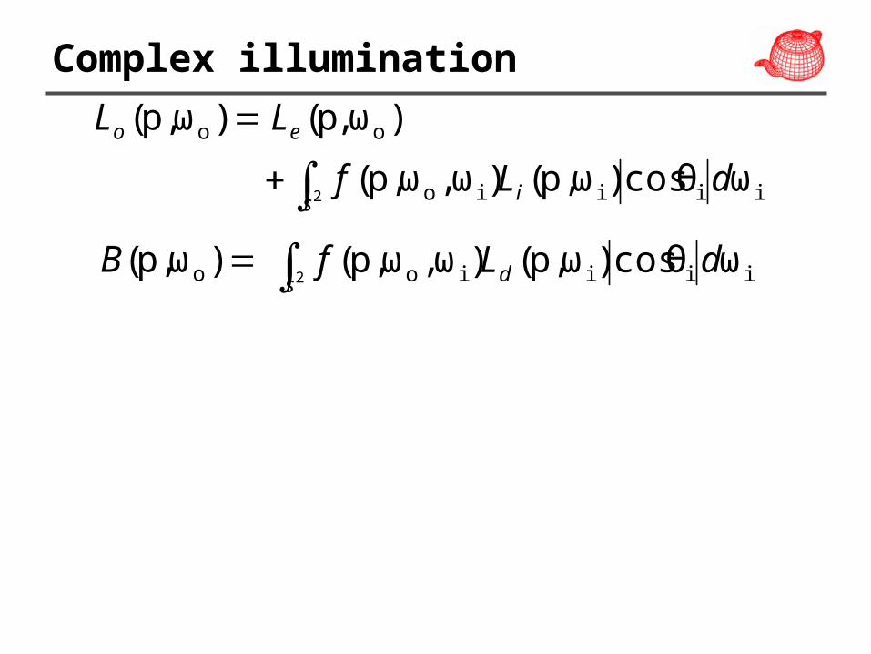
Complex illumination
)ωp,( ooL )ω,p( oeL
iiiio ωθcos)ωp,()ω,ωp,(2
dLf is
)ωp,( oB iiiio ωθcos)ωp,()ω,ωp,(2
dLf ds
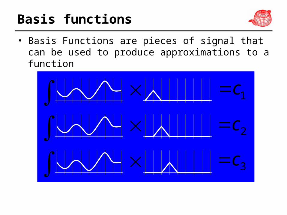
• Basis Functions are pieces of signal that can be used to produce approximations to a function
1c
2c
3c
Basis functions
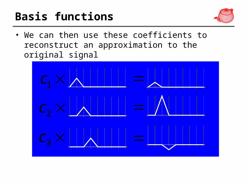
• We can then use these coefficients to reconstruct an approximation to the original signal
1c
2c
3c
Basis functions
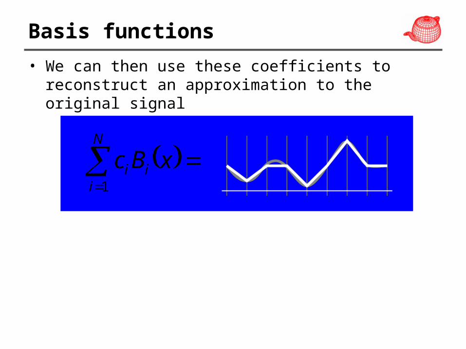
• We can then use these coefficients to reconstruct an approximation to the original signal
xBcN
iii
1
Basis functions
Orthogonal basis functions
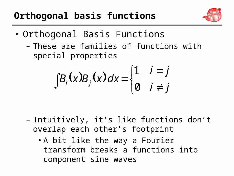
• Orthogonal Basis Functions– These are families of functions with special
properties
– Intuitively, it’s like functions don’t overlap each other’s footprint• A bit like the way a Fourier transform breaks
a functions into component sine waves
ji
jidxxBxB ji 0
1
Basis functions
• Transform data to a space in which we can capture the essence of the data better
• Here, we use spherical harmonics, similar to Fourier transform in spherical domain
Real spherical harmonics
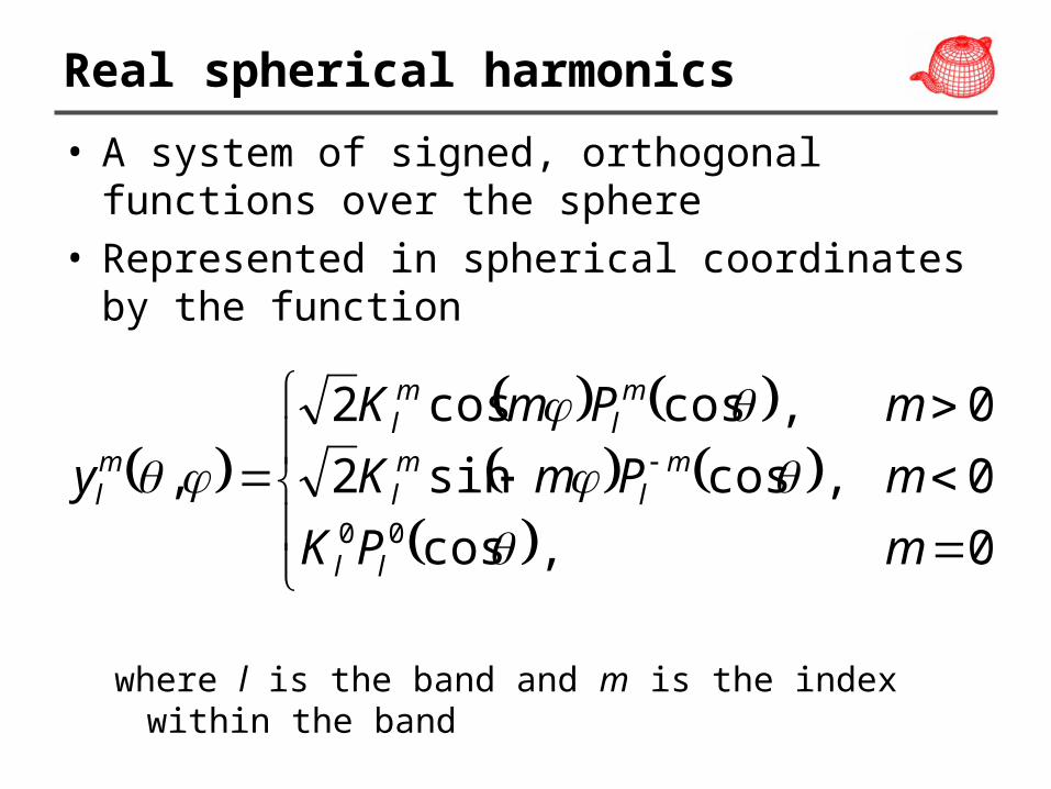
• A system of signed, orthogonal functions over the sphere
• Represented in spherical coordinates by the function
where l is the band and m is the index within the band
0
0
0
,cos
,cossin2
,coscos2
,00 m
m
m
PK
PmK
PmK
y
ll
ml
ml
ml
ml
ml
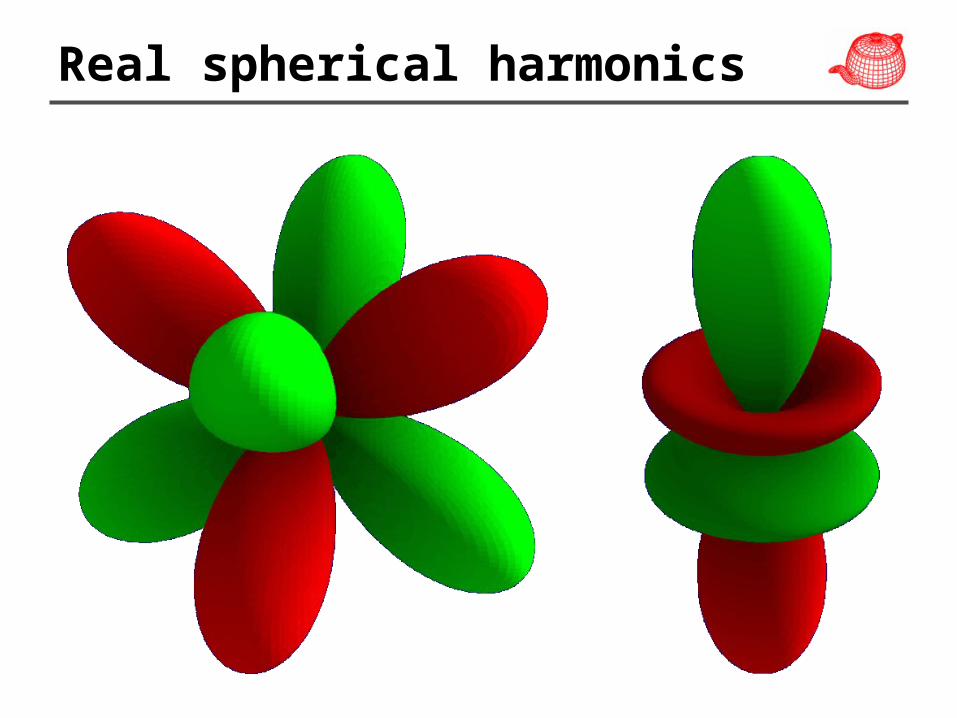
Real spherical harmonics
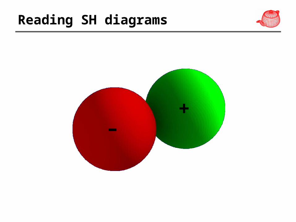
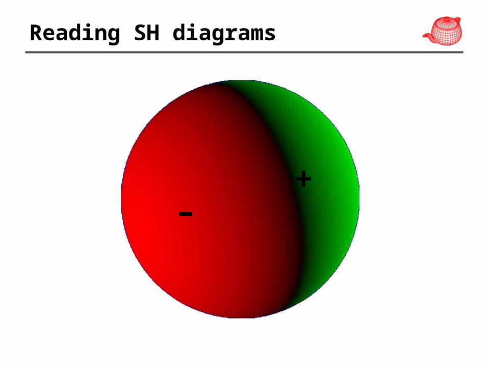
Reading SH diagrams
–+
Not thisdirection
Thisdirection
Reading SH diagrams
–+
Not thisdirection
Thisdirection
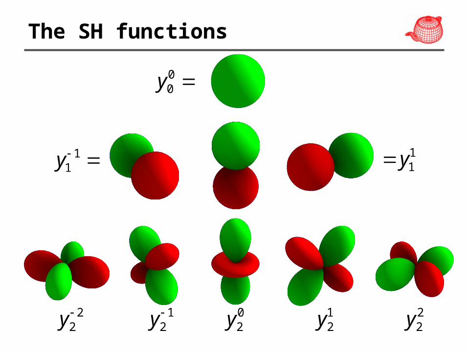
The SH functions
00y
11y
11y
12y
22y
02y
12y2
2y
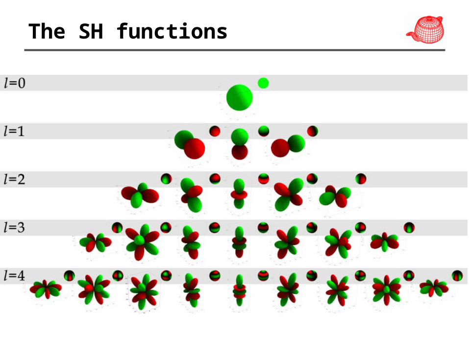
The SH functions
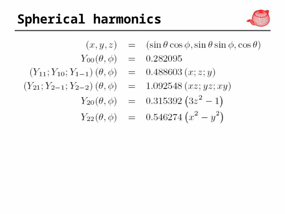
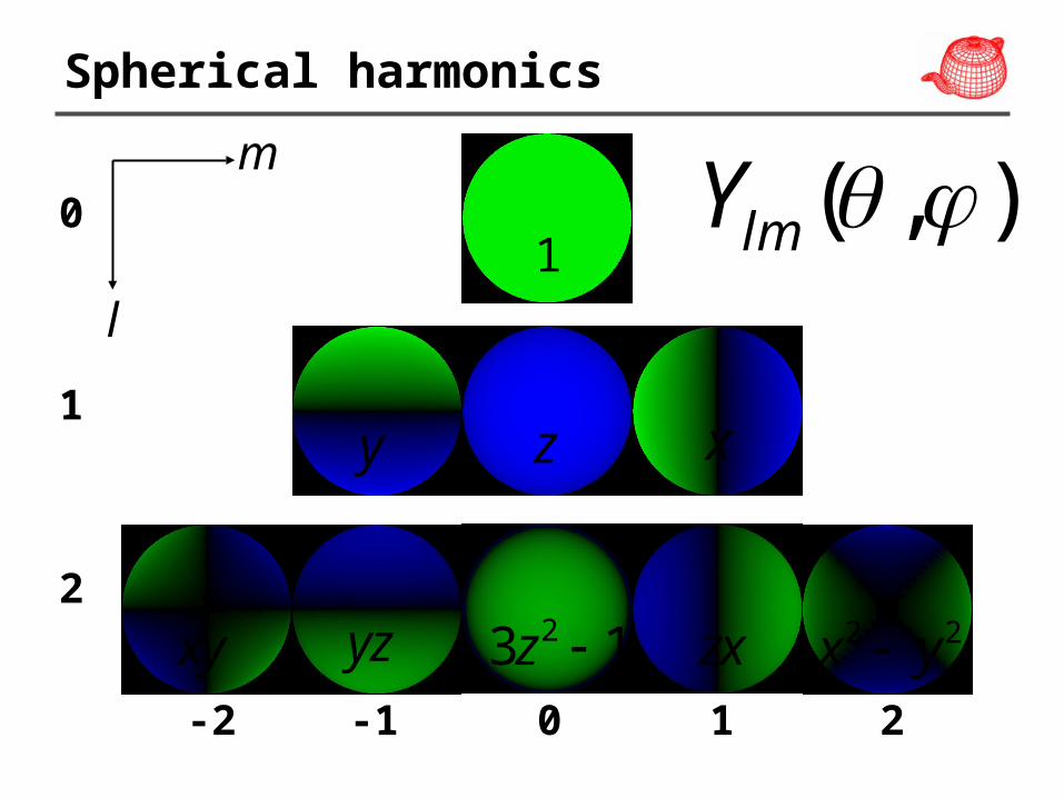
Spherical harmonics
Spherical harmonics
-1-2 0 1 2
0
1
2
( , )lmY
xy z
xy yz 23 1z zx 2 2x y
1
m
l
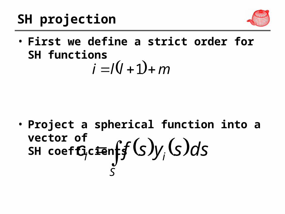
SH projection
• First we define a strict order for SH functions
• Project a spherical function into a vector ofSH coefficients
S
ii dssysfc
mlli 1
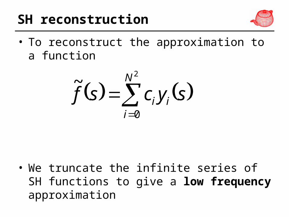
SH reconstruction
• To reconstruct the approximation to a function
• We truncate the infinite series of SH functions to give a low frequency approximation
2
0
~ N
iii sycsf
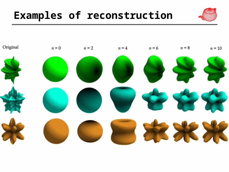
Examples of reconstruction
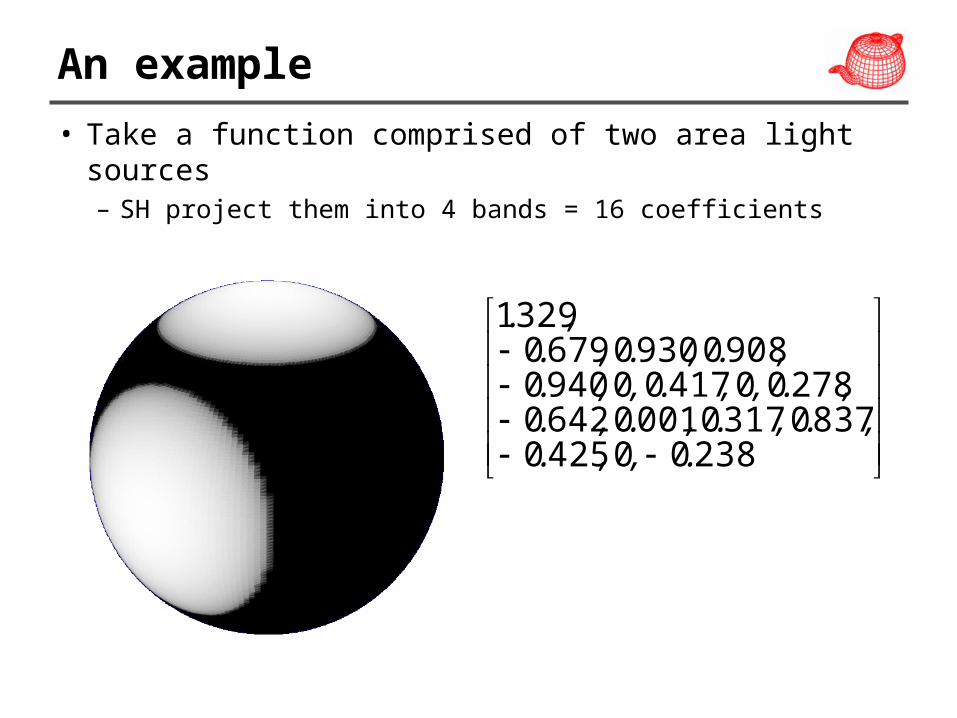
An example
• Take a function comprised of two area light sources– SH project them into 4 bands = 16 coefficients
2380042508370317000106420
27800417009400908093006790
3291
.,,.,.,.,.,.,.,,.,,.
,.,.,.,.
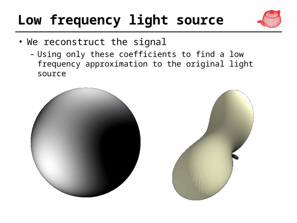
Low frequency light source
• We reconstruct the signal– Using only these coefficients to find a low frequency
approximation to the original light source
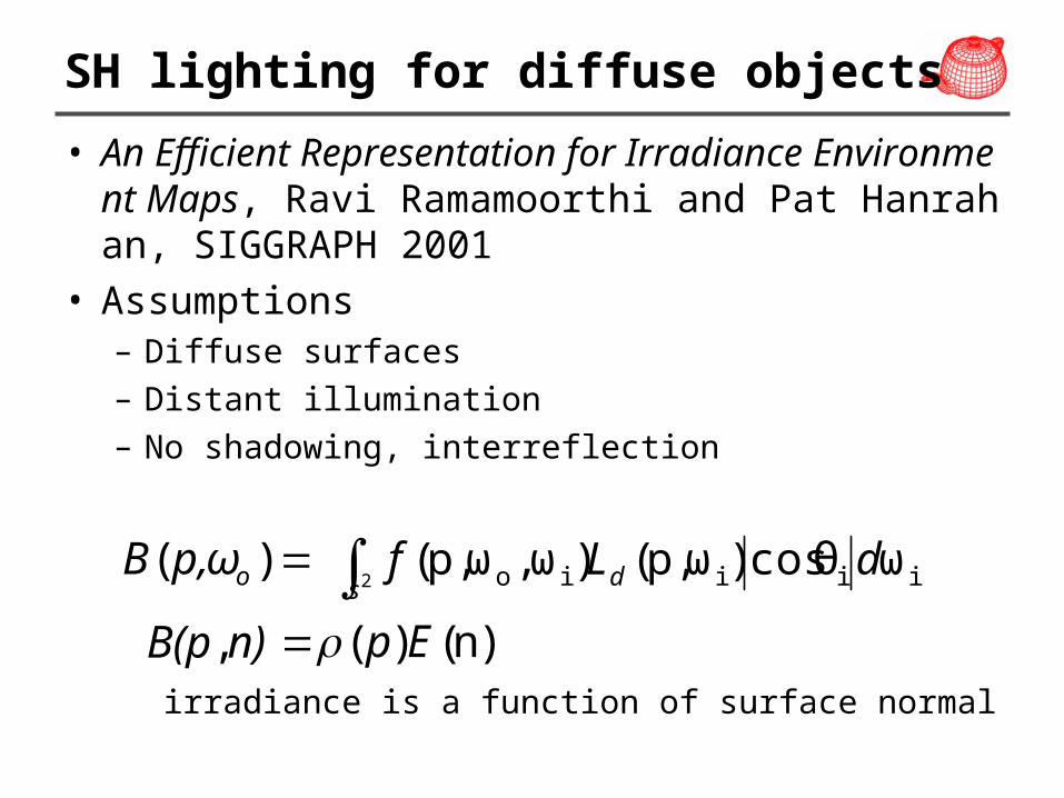
SH lighting for diffuse objects
• An Efficient Representation for Irradiance Environment Maps, Ravi Ramamoorthi and Pat Hanrahan, SIGGRAPH 2001
• Assumptions– Diffuse surfaces– Distant illumination – No shadowing, interreflection
irradiance is a function of surface normal
)( op,ωB iiiio ωθcos)ωp,()ω,ωp,(2
dLf ds)n()( Epn)B(p,
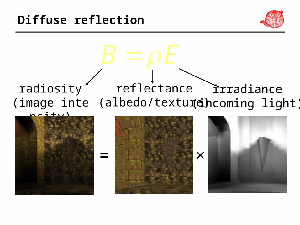
Diffuse reflection
B Eradiosity
(image intensity)reflectance
(albedo/texture)irradiance
(incoming light)
×=
quake light map
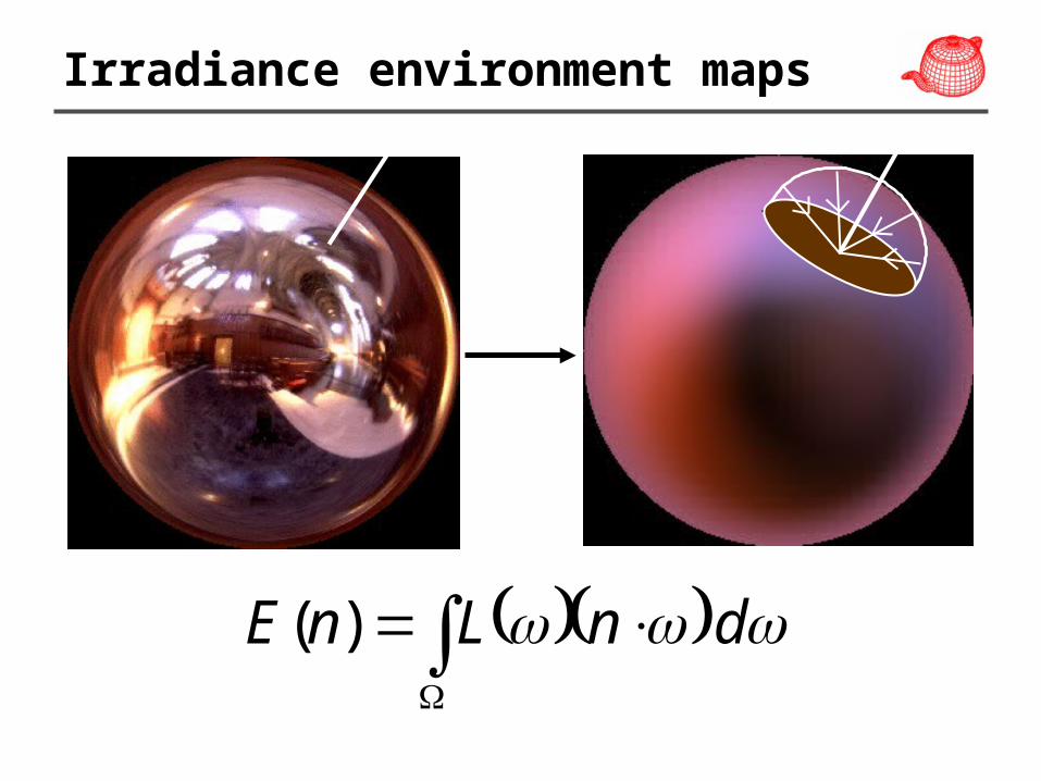
Irradiance environment maps
Illumination Environment Map Irradiance Environment Map
L n
dnLnE )(
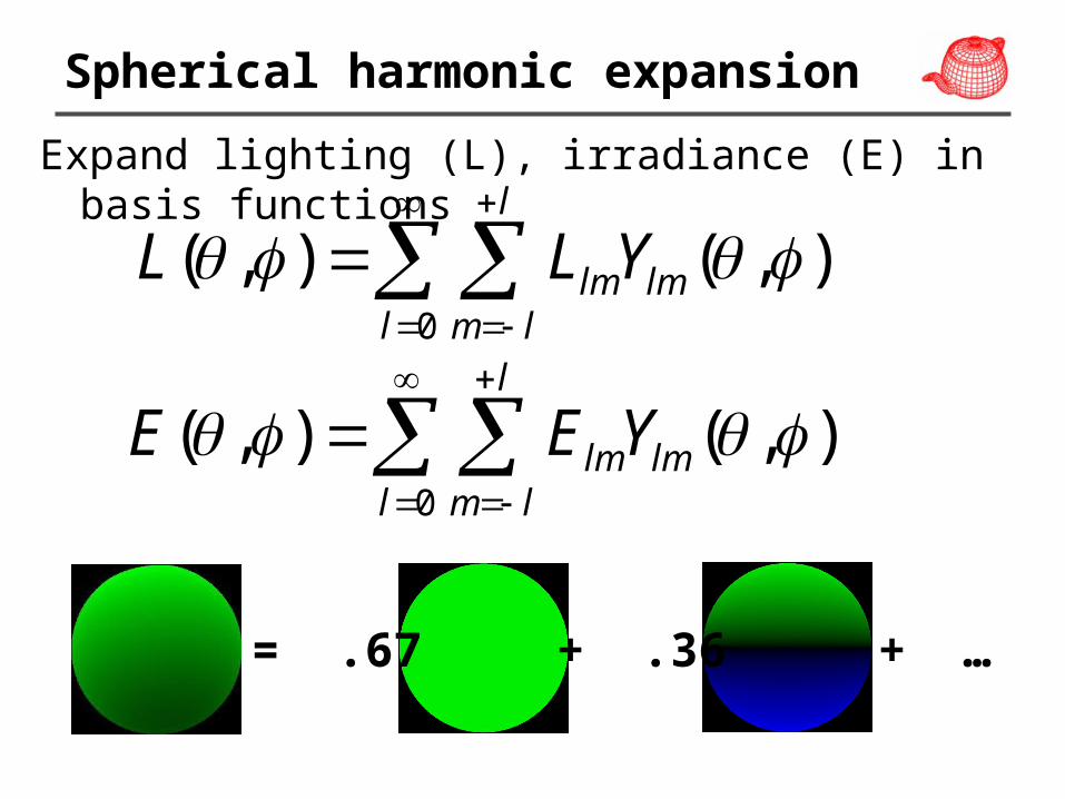
Spherical harmonic expansion
Expand lighting (L), irradiance (E) in basis functions
0
( , ) ( , )l
lm lml m l
L L Y
0
( , ) ( , )l
lm lml m l
E E Y
= .67 + .36 + …
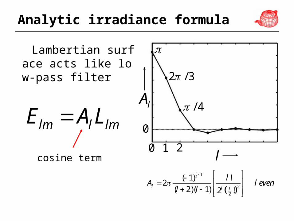
Analytic irradiance formula
Lambertian surface acts like low-pass filter
lm l lmE A LlA
2 / 3
/ 4
0
2 1
2
2
( 1) !2
( 2)( 1) 2 !
l
l l l
lA l even
l l
l0 1 2
cosine term
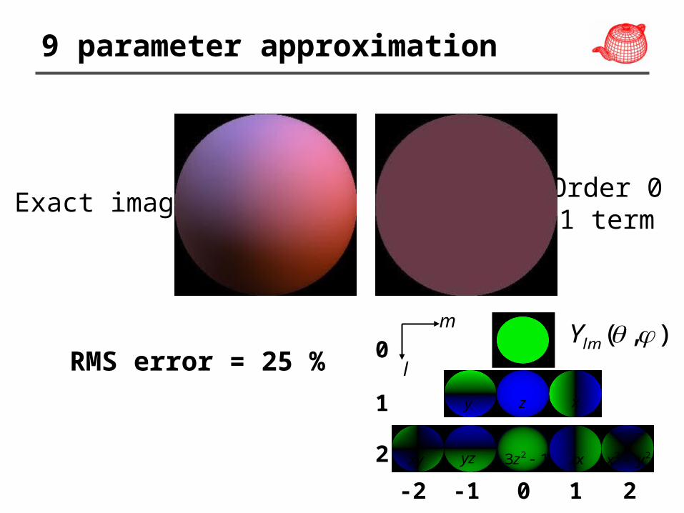
9 parameter approximation
Exact imageOrder 01 term
RMS error = 25 %
-1-2 0 1 2
0
1
2
( , )lmY
xy z
xy yz 23 1z zx 2 2x y
l
m
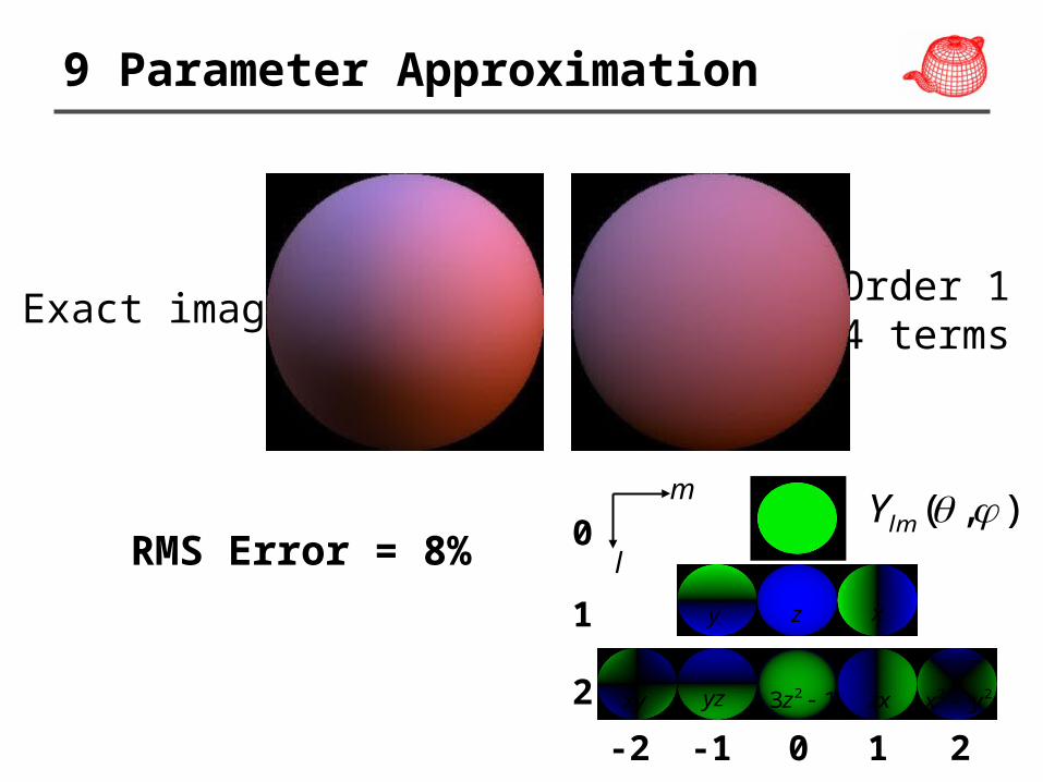
9 Parameter Approximation
Exact imageOrder 14 terms
RMS Error = 8%
-1-2 0 1 2
0
1
2
( , )lmY
xy z
xy yz 23 1z zx 2 2x y
l
m
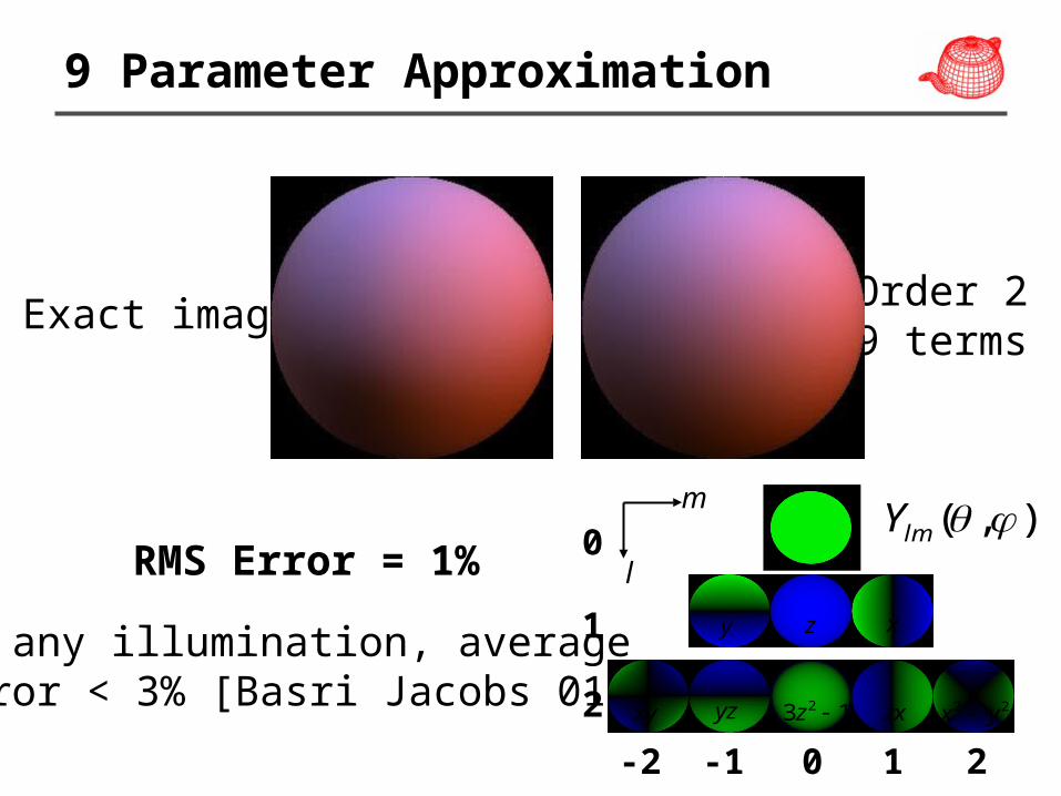
9 Parameter Approximation
Exact imageOrder 29 terms
RMS Error = 1%
For any illumination, average error < 3% [Basri Jacobs 01]
-1-2 0 1 2
0
1
2
( , )lmY
xy z
xy yz 23 1z zx 2 2x y
l
m
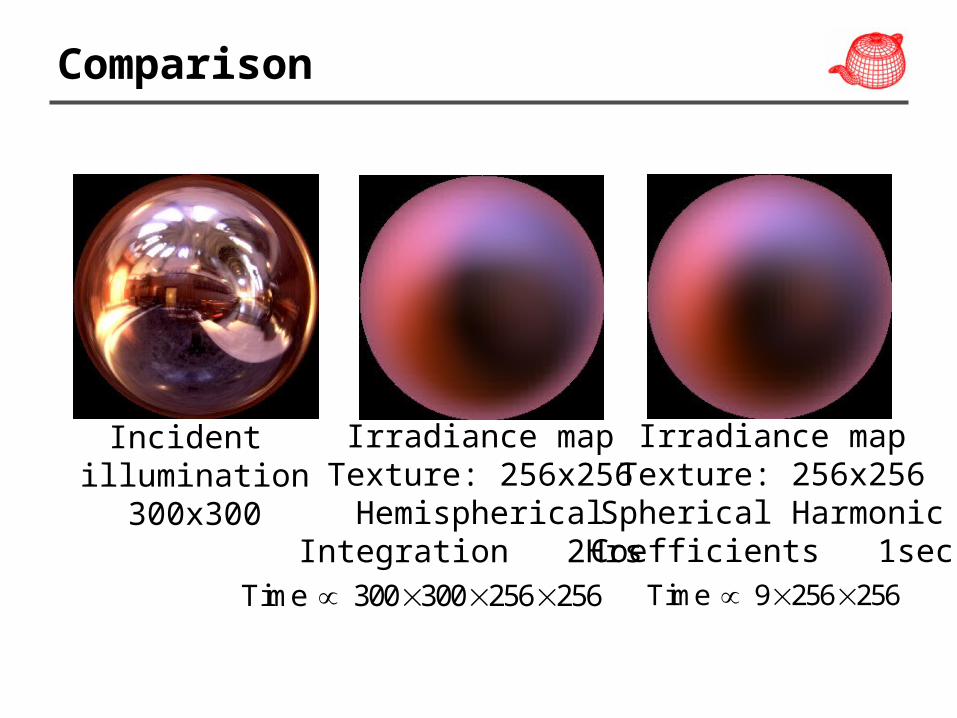
Comparison
Incident illumination
300x300
Irradiance mapTexture: 256x256
HemisphericalIntegration 2Hrs
Irradiance mapTexture: 256x256
Spherical HarmonicCoefficients 1sec
Time 300 300 256 256 Time 9 256 256
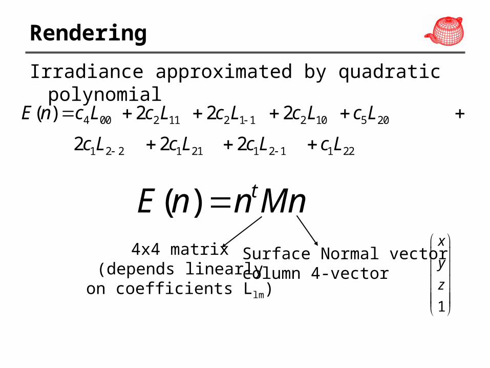
Rendering
Irradiance approximated by quadratic polynomial
24 00 2 11 2 1 1 2 10 5 2
2 2
0
1 2 2 1 21 1 2 1 1 22
1 (3 1( ) 2 2 2
2 2 ( )2
)x y z z
x
E n c L c L c L c L c L
c L c L c Ly xz yz x yc L
( ) tE n n Mn
1
x
y
z
Surface Normal vectorcolumn 4-vector
4x4 matrix(depends linearly
on coefficients Llm)
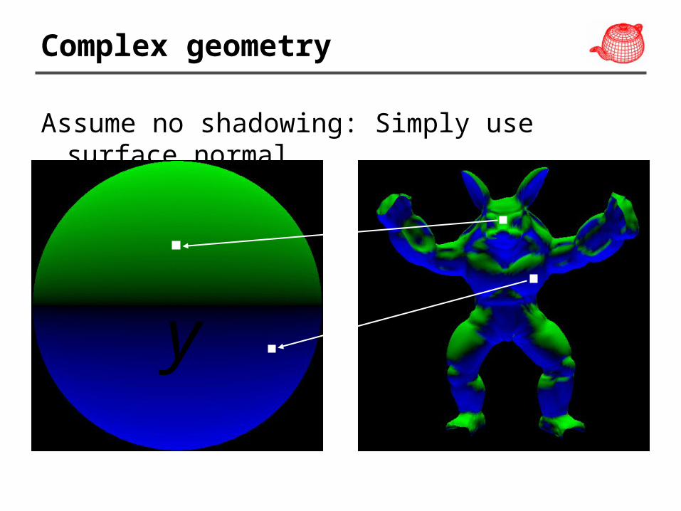
Complex geometry
Assume no shadowing: Simply use surface normal
y
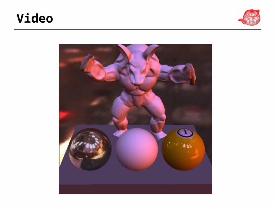
Video